epa qa/g-9r · agency washington, dc 20460 data quality assessment: a reviewer’s guide epa...
TRANSCRIPT

United States Office of Environmental EPA/240/B-06/002 Environmental Protection Information February 2006 Agency Washington, DC 20460
Data Quality Assessment: A Reviewer’s Guide
EPA QA/G-9R


EPA QA/G-9R February 2006 iii
FOREWORD
This document is the 2006 version of the Data Quality Assessment: A Reviewer’s Guide which provides general guidance to organizations on assessing data quality criteria and performance specifications for decision making. The Environmental Protection Agency (EPA) has developed a process for performing the Data Quality Assessment (DQA) Process for project managers and planners to determine whether the type, quantity, and quality of data needed to support Agency decisions have been achieved. This guidance is the culmination of experiences in the design and statistical analyses of environmental data in different Program Offices at the EPA. Many elements of prior guidance, statistics, and scientific planning have been incorporated into this document.
This document is one of a series of quality management guidance documents that the EPA Quality Staff has prepared to assist users in implementing the Agency-wide Quality System. Other related documents include:
EPA QA/G-4 Guidance on Systematic Planning using the Data Quality Objectives Process
EPA QA/G-4D DEFT Software for the Data Quality Objectives Process
EPA QA/G-5S Guidance on Choosing a Sampling Design for Environmental Data Collection
EPA QA/G-9S Data Quality Assessment: Statistical Methods for Practitioners
This document is intended to be a "living document" that will be updated periodically to
incorporate new topics and revisions or refinements to existing procedures. Comments received on this 2006 version will be considered for inclusion in subsequent versions. Please send your written comments on the Data Quality Assessment: A Reviewer’s Guide to:
Quality Staff (2811R) Office of Environmental Information U.S. Environmental Protection Agency 1200 Pennsylvania Avenue N.W. Washington, DC 20460 Phone: (202) 564-6830 Fax: (202) 565-2441 E-mail: [email protected]

EPA QA/G-9R February 2006 iv

EPA QA/G-9R February 2006 v
TABLE OF CONTENTS
Page INTRODUCTION .......................................................................................................................... 1
0.1 Purpose of this Guidance ................................................................................................ 1 0.2 DQA and the Data Life Cycle......................................................................................... 2 0.3 The Five Steps of Statistical DQA.................................................................................. 3 0.4 Intended Audience .......................................................................................................... 4 0.5 Organization of this Guidance ........................................................................................ 5
STEP 1: REVIEW THE PROJECT’S OBJECTIVES AND SAMPLING DESIGN.................... 7 1.1 Review Study Objectives................................................................................................ 8 1.2 Translate Study Objectives into Statistical Terms .......................................................... 8 1.3 Developing Limits on Uncertainty.................................................................................. 9 1.4 Review Sampling Design.............................................................................................. 10 1.5 What Outputs Should a DQA Reviewer Have at the Conclusion of Step 1? ............... 12
STEP 2: CONDUCT A PRELIMINARY DATA REVIEW....................................................... 13 2.1 Review Quality Assurance Reports .............................................................................. 13 2.2 Calculate Basic Statistical Quantities ........................................................................... 14 2.3 Graph the Data .............................................................................................................. 14 2.4 What Outputs Should a DQA Reviewer Have at the Conclusion of Step 2? ............... 14
STEP 3: SELECT THE STATISTICAL METHOD ................................................................... 15 3.1 Choosing Between Alternatives: Hypothesis Testing................................................... 15 3.2 Estimating a Parameter: Confidence Intervals and Tolerance Intervals ....................... 17 3.3 What Output Should a DQA Reviewer Have at the Conclusion of Step 3? ................. 17
STEP 4: VERIFY THE ASSUMPTIONS OF THE STATISTICAL METHOD........................ 19 4.1 Perform Tests of Assumptions...................................................................................... 19 4.2 Develop an Alternate Plan ............................................................................................ 20 4.3 Corrective Actions ........................................................................................................ 20 4.4 What Outputs Should a DQA Reviewer Have at the End of Step 4? ........................... 20
STEP 5: DRAW CONCLUSIONS FROM THE DATA............................................................. 21 5.1 Perform the Statistical Method ..................................................................................... 21 5.2 Draw Study Conclusions............................................................................................... 21 5.3 Hypothesis Tests ........................................................................................................... 21 5.4 Confidence Intervals ..................................................................................................... 23 5.5 Tolerance Intervals........................................................................................................ 23 5.6 Evaluate Performance of the Sampling Design ............................................................ 24 5.7 What Output Should the DQA Reviewer Have at the End of Step 5?.......................... 24
INTERPRETING AND COMMUNICATING THE TEST RESULTS....................................... 25 6.1 Data Interpretation: The Meaning of p-values............................................................. 25 6.2 Data Interpretation: "Accepting" vs. "Failing to Reject" the Null Hypothesis............. 26 6.3 Data Sufficiency: "Proof of Safety" vs. "Proof of Hazard" ......................................... 26 6.4 Data Sufficiency: Quantity vs. Quality of Data ........................................................... 28 6.5 Data Sufficiency: Statistical Significance vs. Practical Significance .......................... 28 6.6 Conclusions................................................................................................................... 29
REFERENCES ............................................................................................................................. 25

EPA QA/G-9R February 2006 vi
Page Appendix A: Commonly Used Statistical Quantities .................................................................. 33 Appendix B: Graphical Representation of Data .......................................................................... 37 Appendix C: Common Hypothesis Tests..................................................................................... 43 Appendix D: Commonly Used Statements of Hypotheses .......................................................... 47 Appendix E: Common Assumptions and Transformations ......................................................... 49 Appendix F: Checklist of Outputs for Data Quality Assessment ................................................ 55

EPA QA/G-9R February 2006 1
CHAPTER 0
INTRODUCTION 0.1 Purpose of this Guidance
Data Quality Assessment (DQA) is the scientific and statistical evaluation of environmental data to determine if they meet the planning objectives of the project, and thus are of the right type, quality, and quantity to support their intended use. This guidance describes broadly the statistical aspects of DQA in evaluating environmental data sets. A more detailed discussion about DQA graphical and statistical tools may be found in the companion guidance document, Data Quality Assessment: Statistical Methods for Practitioners (Final Draft) (EPA QA/G-9S) (U.S. EPA 2004). This guidance applies to using DQA to support environmental decision-making (e.g., compliance determinations), and to using DQA in estimation problems in which environmental data are used (e.g., monitoring programs).
DQA is built on a fundamental premise: data quality is meaningful only when it relates to
the intended use of the data. Data quality does not exist in a vacuum, a reviewer needs to know in what context a data set is to be used in order to establish a relevant yardstick for judging whether or not the data is acceptable. By using DQA, a reviewer can answer four important questions:
1. Can a decision (or estimate) be made with the desired level of certainty, given the
quality of the data? 2. How well did the sampling design perform? 3. If the same sampling design strategy is used again for a similar study, would the
data be expected to support the same intended use with the desired level of certainty?
4. Is it likely that sufficient samples were taken to enable the reviewer to see an
effect if it was really present?
The first question addresses the reviewer’s immediate needs. For example, if the data are being used for decision-making and provide evidence strongly in favor of one course of action over another, then the decision maker can proceed knowing that the decision will be supported by unambiguous data. However, if the data do not show sufficiently strong evidence to favor one alternative, then the data analysis alerts the decision maker to this uncertainty. The decision maker now is in a position to make an informed choice about how to proceed (such as collect more or different data before making the decision, or proceed with the decision despite the relatively high, but tolerable, chance of drawing an erroneous conclusion).
The second question addresses how robust this sampling design is with respect to changing conditions. If the design is very sensitive to potentially disturbing influences, then

EPA QA/G-9R February 2006 2
interpretation of the results may be difficult. By addressing the second question the reviewer guards against the possibility of a spurious result arising from a unique set of circumstances.
The third question addresses the problem of whether this could be considered a unique situation where the results of this DQA only applies to this situation only and the conclusions cannot be extrapolated to similar situations. It also addresses the suitability of using this data collection design cannot reviewer’s potential future needs. For example, if reviewers intend to use a certain sampling design at a different location from where the design was first used, they should determine how well the design can be expected to perform given that the outcomes and environmental conditions of this sampling event will be different from those of the original event. As environmental conditions will vary from one location or one time to another, the adequacy of the sampling design should be evaluated over a broad range of possible outcomes and conditions.
The final question addresses the issue of whether sufficient resources were used in the
study. For example, in an epidemiological investigation, was it likely the effect of interest could be reliably observed given the limited number of samples actually obtained.
0.2 DQA and the Data Life Cycle
The data life cycle (depicted in Figure 0-1) comprises three steps: planning,
implementation, and assessment. During the planning phase, a systematic planning procedure (such as the Data Quality Objectives (DQO) Process) is used to define criteria for determining the number, location, and timing of samples (measurements) to be collected in order to produce a result with a desired level of certainty.
This information, along with the sampling methods, analytical procedures, and appropriate quality assurance (QA) and quality control procedures, is documented in the QA Project Plan. Data are then collected following the QA Project Plan specifications in the implementation phase.
At the outset of the assessment phase, the data are verified and validated to ensure that
the sampling and analysis protocols specified in the QA Project Plan were followed, and that the measurement systems were performed in accordance with the criteria specified in the QA Project Plan. Then the statistical component of DQA completes the data life cycle by providing the evaluation needed to determine if the performance and acceptance criteria developed by the DQO planning process were achieved.

EPA QA/G-9R February 2006 3
Figure 0-1. Data Life Cycle 0.3 The Five Steps of Statistical DQA
The statistical part of DQA involves five steps that begin with a review of the planning documentation and end with an answer to the problem or question posed during the planning phase of the study. These steps roughly parallel the actions of an environmental statistician when analyzing a set of data. The five steps, which are described in more detail in the following chapters of this guidance, are briefly summarized as follows:
1. Review the project’s objectives and sampling design: Review the objectives
defined during systematic planning to assure that they are still applicable. If objectives have not been developed (e.g., when using existing data independently collected), specify them before evaluating the data for the projects objectives. Review the sampling design and data collection documentation for consistency with the project objectives observing any potential discrepancies.
2. Conduct a preliminary data review: Review QA reports (when possible) for the
validation of data, calculate basic statistics, and generate graphs of the data. Use this information to learn about the structure of the data and identify patterns, relationships, or potential anomalies.
3. Select the statistical method: Select the appropriate procedures for summarizing
and analyzing the data, based on the review of the performance and acceptance
IMPLEMENTATIONField Data Collection and Associated
Quality Assurance / Quality Control Activities
PLANNINGData Quality Objectives Process
Quality Assurance Project Plan Development
ASSESSMENTData Verification/ ValidationData Quality Assessment
OUTPUT
INPUT
OUTPUT
QUALITY ASSURANCE ASSESSMENT
PROJECT CONCLUSIONS
DATA VERIFICATION /VALIDATION
• Verify measurement performance
• Verify measurement procedures and reporting specifications
VERIFIED /VALIDATED DATA
DATA QUALITY ASSESSMENT
• Review project objectives and
• Conduct preliminary data review
• Select statistical method
• Verify assumptions of the method
• Draw conclusions from the data
QC/PerformanceEvaluation DataRoutine Data
INPUTS
sampling design

EPA QA/G-9R February 2006 4
criteria associated with the projects objectives, the sampling design, and the preliminary data review. Identify the key underlying assumptions associated with the statistical test.
4. Verify the assumptions of the statistical method: Evaluate whether the
underlying assumptions hold, or whether departures are acceptable, given the actual data and other information about the study.
5. Draw conclusions from the data: Perform the calculations pertinent to the
statistical test, and document the conclusions to be drawn as a result of these calculations. If the design is to be used again, evaluate the performance of the sampling design.
Although these five steps are presented in a linear sequence, DQA is by its very nature
iterative. For example, if the preliminary data review reveals patterns or anomalies in the data set that are inconsistent with the project objectives, then some aspects of the study analysis may have to be reconsidered. Likewise, if the underlying assumptions of the statistical test are not supported by the data, then previous steps of the DQA may have to be revisited. The strength of DQA Process is that it is designed to promote an understanding of how well the data satisfy their intended use by progressing in a logical and efficient manner. Nevertheless, it should be realized that DQA cannot absolutely prove that the objectives set forth in the planning phase of a study have been achieved. This is because the reviewer can never know the true value of the item of interest, only information from a sample. Sample data collection provides the reviewer only with an estimate, not the true value. As an reviewer makes a determination based on the estimated value, there is always the risk of drawing an incorrect conclusion. Use of a well-documented planning process helps reduce this risk to an acceptable level. 0.4 Intended Audience
This guidance is written as a general overview of statistical DQA for a broad audience of potential data users, reviewers, data generators and data investigators. Reviewers (such as project managers, risk assessors, or principal investigators who are responsible for making decisions or producing estimates regarding environmental characteristics based on environmental data) should find this guidance useful for understanding and directing the technical work of others who produce and analyze data. Data generators (such as analytical chemists, field sampling specialists, or technical support staff responsible for collecting and analyzing environmental samples and reporting the resulting data values) should find this guidance helpful for understanding how their work will be used. Data investigators (such as technical investigators responsible for evaluating the quality of environmental data) should find this guidance to be a handy summary of DQA-related concepts. Specific information about applying DQA-related graphical and statistical techniques is contained in the companion guidance, Data Quality Assessment: Statistical Methods for Practitioners (Final Draft) (EPA QA/G-9S).

EPA QA/G-9R February 2006 5
0.5 Organization of this Guidance
Chapters 1 through 5 of this guidance address the five steps of DQA in turn. Each chapter discusses the activities expected and includes a list of the outputs that should be achieved in that step. Chapter 6 provides additional perspectives on how to interpret data and understand/ communicate the conclusions drawn from data. Finally, Appendices A through E contain non-technical explanatory material describing some of the statistical concepts used. Appendix F is a checklist that can be used to ensure all steps of the DQA process have been addressed.

EPA QA/G-9R February 2006 6

EPA QA/G-9R February 2006 7
Step 1. State the Problem
Define the problem that motivates the Identify the planning team; examine budget, schedule.
Step 2. Identify the Goal of the StudyState how environmental data will be used in solving theproblem; identify study questions; define alternative outcomes.
Step 3. Identify Information Inputs
Step 4. Define the Boundaries of the StudySpecify the target population and characteristics of interest;define spatial and temporal limits, scale of inference.
Step 5. Develop the Analytic ApproachDefine the parameter of interest; specify the type of inference and develop logic for drawing conclusions from the findings.
Develop performance criteria for new data being collected,
Select the most resource-
Statistical Estimation and other analytical approaches
Step 1. State the ProblemDefine the problem that motivates the study;Identify the planning team; examine budget, s
Step 2. Identify the Goal of the StudyState how environmental data will be used in solving the
Step 3. Identify Information InputsIdentify data and information needed to answer study questions.
Step 4. Define the Boundaries of the StudySpecify the target population and characteristics of interest;define spatial and temporal limits, scale of inference.
Step 5. Develop the Analytic ApproachDefine the parameter of interestand develop logic for drawing conclusions from the findings.
Step 6. Specify Performance or Acceptance CriteriaDevelop performance criteria for new data being collected, acceptance criteria for data already collected.
Step 7. Develop the Detailed Plan for Obtaining DataSelect the most resource effective sampling and analysis plan-that satisfies the performance or acceptance criteria.
StatisticalHypothesis Testing
Estimation and other
Step 1. State the ProblemDefine the problem that motivates the Identify the planning team; examine budget, schedule.
Step 2. Identify the Goal of the StudyState how environmental data will be used in solving theproblem; identify study questions; define alternative outcomes.
Step 3. Identify Information Inputs
Step 4. Define the Boundaries of the StudySpecify the target population and characteristics of interest;define spatial and temporal limits, scale of inference.
Step 5. Develop the Analytic ApproachDefine the parameter of interest; specify the type of inference and develop logic for drawing conclusions from the findings.
Develop performance criteria for new data being collected,
Select the most resource-
Statistical Estimation and other analytical approaches
Step 1. State the ProblemDefine the problem that motivates the study;Identify the planning team; examine budget, s
Step 2. Identify the Goal of the StudyState how environmental data will be used in solving the
Step 3. Identify Information InputsIdentify data and information needed to answer study questions.
Step 4. Define the Boundaries of the StudySpecify the target population and characteristics of interest;define spatial and temporal limits, scale of inference.
Step 5. Develop the Analytic ApproachDefine the parameter of interestand develop logic for drawing conclusions from the findings.
Step 6. Specify Performance or Acceptance CriteriaDevelop performance criteria for new data being collected, acceptance criteria for data already collected.
Step 7. Develop the Detailed Plan for Obtaining DataSelect the most resource effective sampling and analysis plan-that satisfies the performance or acceptance criteria.
StatisticalHypothesis Testing
Estimation and other
Figure 1-1. The Data Quality Objectives Process
CHAPTER 1
STEP 1: REVIEW THE PROJECT’S OBJECTIVES AND SAMPLING DESIGN DQA begins by reviewing the key outputs from the planning phase of the data life cycle such as the Data Quality Objectives, the QA Project Plan, and any related documents. The study objective provides the context for understanding the purpose of the data collection effort and establishes the qualitative and quantitative basis for assessing the quality of the data set for the intended use. The sampling design (documented in the QA Project Plan) provides important information about how to interpret the data. By studying the sampling design, the reviewer can gain an understanding of the assumptions under which the design was developed, as well as the relationship between these assumptions and the study objective. By reviewing the methods by which the samples were collected, measured, and reported, the reviewer prepares for the preliminary data review and subsequent steps of DQA. Systematic planning improves the representativeness and overall quality of a sampling design, the effectiveness and efficiency with which the sampling and analysis plan is implemented, and the usefulness of subsequent DQA efforts. For systematic planning, the Agency recommends the DQO Process, a logical, systematic planning process based on the scientific method. The DQO Process emphasizes the planning and development of a sampling design to collect the right type, quality, and quantity of data for the intended use. Employing both the DQO Process and DQA will help to ensure that projects are supported by data of adequate quality; the DQO Process does so prospectively and DQA does so retrospectively. Systematic planning, whether the DQO Process or other, can help assure that data are not collected spuriously. The DQO Process is discussed in Guidance on the Data Quality Objectives Process (QA/G-4) (U.S. EPA 2000a). In instances where project objectives have not been developed and documented during the planning phase of the study, it is necessary to recreate some of the project objectives prior to conducting the DQA. These are used to make appropriate criteria for evaluating the quality of the data with respect to their intended use. The most important recreations are: hypotheses chosen, level of significance selected (tolerable levels of potential decision errors), statistical method selected, and number of samples collected. The seven steps of the DQO Process are illustrated in Figure 1-1.

EPA QA/G-9R February 2006 8
1.1 Review Study Objectives
First, the objectives of the study should be reviewed in order to provide a context for analyzing the data. If a systematic planning process has been implemented before the data are collected, then this step reduces to reviewing the documentation on the study objectives. If no clear planning process was used, the reviewer should:
• Develop a concise definition of the problem (e.g. DQO Process Step 1) and of the
methodology of how the data were collected (e.g. DQO Process Step 2). This should provide the fundamental reason for collecting the environmental data and identify all potential actions that could result from the data analysis.
• Identify the target population (universe of interest) and determine if any essential information is missing (e.g. DQO Process Step 3). If so, either collect the missing information before proceeding, or select a different approach to resolving the problem.
• Specify the scale of determination (any subpopulations of interest) and any boundaries on the study (e.g. DQO Process Step 4) based on the sampling design. The scale of determination is the smallest area or time period to which the conclusions of the study will apply. The apparent sampling design and implementation may restrict how small or how large this scale of determination can be.
1.2 Translate Study Objectives into Statistical Terms In this activity, the reviewer's objectives are used to develop a precise statement of how environmental data will be evaluated to generate the study’s conclusions. If DQOs were generated during planning, this statement will be found as an output of DQO Process Step 5.
In many cases, this activity is best accomplished by the formulation of statistical hypotheses, including a null hypothesis, which is a "baseline condition" that is presumed to be true in the absence of strong evidence to the contrary, as well as an alternative hypothesis, which bears the burden of proof. In other words, the baseline condition will be retained unless the alternative condition (the alternative hypothesis) is thought to be true due to the preponderance of evidence. In general, such hypotheses often consist of the following elements:
• a population parameter of interest (such as a mean or a median), which describes the
feature of the environment that the reviewer is investigating;
• a numerical value to which the parameter will be compared, such as a regulatory or risk-based threshold or a similar parameter from another place (e.g., comparison to a reference site) or time (e.g., comparison to a prior time); and

EPA QA/G-9R February 2006 9
• a relationship (such as "is equal to" or "is greater than") that specifies precisely how the parameter will be compared to the numerical value.
Section 3.1 provides additional information on how to develop the statement of hypotheses, and includes a list of commonly encountered hypotheses for environmental projects. Some environmental data collection efforts do not involve the direct comparison of measured values to a fixed value. For instance, for monitoring programs or exploratory studies, the goal may be to develop estimates of values or ranges applicable to given parameters. This is best accomplished by the formulation of confidence intervals or tolerance intervals, which estimate the probability that the true value of a parameter is within a given range. In general, confidence intervals consist of the following elements:
• a range of values with in which the unknown population parameter of interest (such as the mean or median) is thought to lie; and
• a probabilistic expression denoting the chance that this range captures the parameter of
interest. An example of a confidence interval would be ‘We are 95% confident that the interval 47.3 to 51.8 contains the population mean.’
Tolerance intervals are used with proportions. Here, we wish to have a certain level of confidence that a certain proportion of the population falls in a certain region. An example of a tolerance interval would be ‘We are 95% confident that at least 80% of the population is above the threshold value.’ Section 3.2 provides additional information on confidence intervals and tolerance intervals.
For discussion of technical issues related to statistical testing using hypotheses or confidence/tolerance intervals, refer to Chapter 3 of Data Quality Assessment: Statistical Methods for Practitioners (Final Draft) (EPA QA/G-9S). 1.3 Developing Limits on Uncertainty The goal of this activity is to develop quantitative statements of the reviewer’s tolerance for uncertainty in conclusions drawn from the data and in actions based on those conclusions. These statements are generated during DQO Process Step 6, but they can also be generated retrospectively as part of DQA.
If the project has been framed as a hypothesis test, then the uncertainty limits can be expressed as the reviewer's tolerance for committing false rejection (Type I, sometimes called a false positive) or false acceptance (Type II, sometimes called a false negative) decision errors1. 1 Decision errors occur when the data collected do not adequately represent the population of interest. For example, the limited amount of information collected may have a preponderance of high values that were sampled by pure

EPA QA/G-9R February 2006 10
A false rejection error occurs when the null hypothesis is rejected when it is, in fact, true. A false acceptance error occurs when the null hypothesis is not rejected (often called “accepted”) when it is, in fact, false. Other related phrases in common use include "level of significance" which is equal to the Type I error (false rejection) rate, and "power" which is equal to 1 - Type II error (false acceptance) rate. When a hypothesis is being tested, it is convenient to summarize the applicable uncertainty limits by means of a “decision performance goal diagram”. For detailed information on how to develop false rejection and false acceptance decision error rates, see Chapter 6 of Guidance on the Data Quality Objectives Process (QA/G-4) (U.S. EPA 2000a).
If the project has been framed in terms of confidence intervals, then uncertainty is expressed as a combination of two interrelated terms:
• the width of the interval (smaller intervals correspond to a smaller degree of uncertainty); and
• the confidence level (typically stated as a percentage) indicating the chance this
interval captures the unknown parameter of interest (a 95% confidence level represents a smaller degree of uncertainty than, say, a 90% confidence level).
If the project has been framed in terms of tolerance intervals, then uncertainty is
expressed as a combination of confidence level and:
• the proportion of the population that lies in the interval.
Note that there is nothing inherently preferable about obtaining a particular probability, such as 95% for the confidence interval. For the same data set, there can be a 95% probability that the parameter lies within a given interval, as well as a 90% probability that it lies within another (smaller) interval, and an 80% probability of being in even a smaller interval. All the intervals are centered on the best estimate of that parameter usually calculated directly from the data (see also Chapter 3.2). 1.4 Review Sampling Design The goal of this activity is to familiarize the reviewer with the main features of the sampling design that was used to generate the environmental data. If DQOs were developed during planning, the sampling design will have been summarized as part of DQO Process Step 7. The design and sampling strategy should be discussed in clear detail in the QA Project Plan or Sampling and Analysis Plan. The overall type of sampling design and the manner in which samples were collected or measurements were taken will place conditions and constraints on how the data can be used and interpreted.
chance. A decision maker could possibly draw the conclusion (decision) that the target population was high when, in fact, it was much lower. A similar situation occurs when the data are collected according to a plan that is too limited to reflect the true underlying variability.

EPA QA/G-9R February 2006 11
The key distinction in sampling design is between judgmental (also called authoritative) sampling (in which sample numbers and locations are selected based on expert knowledge of the problem) and probability sampling (in which sample numbers and locations are selected based on randomization, and each member of the target population has a known probability of being included in the sample).
Judgmental sampling has some advantages and is appropriate in some cases, but the reviewer should be aware of its limitations and drawbacks. This type of sampling should be considered only when the objectives of the investigation are not of a statistical nature (for example, when the objective of a study is to identify specific locations of leaks, or when the study is focused solely on the sampling locations themselves). Generally, conclusions drawn from judgmental samples apply only to those individual samples; aggregation may result in severe bias due to lack of representativeness and lead to highly erroneous conclusions. Judgmental sampling, although often rapid to implement, precludes the use of the sample for any purpose other than the original one.
If the reviewer elects to proceed with judgmental data, then great care should be taken in interpreting any statistical statements concerning the conclusions to be drawn. Using a probabilistic statement with a judgmental sample is incorrect and should be avoided as it gives an illusion of correctness where there is none. The further the judgmental sample is from a truly random sample, the more questionable the conclusions.
Probabilistic sampling is often more difficult to implement than judgmental sampling due to the difficulty of locating the random locations of the samples. It does have the advantage of allowing probability statements to be made about the quality of estimates or hypothesis tests that are derived from the resultant data. One common misconception of probability sampling procedures is that these procedures preclude the use of expert knowledge or important prior information about the problem. Indeed, just the opposite is true; an efficient sampling design is one that uses all available prior information to stratify the region (in order to improve the representativeness of the resulting samples) and set appropriate probabilities of selection.
Common types of probabilistic sampling designs include the following:
• Simple random sampling – the method of sampling where samples are collected at random times or locations throughout the sampling period or study area.
• Stratified sampling – a sampling method where a population is divided into non-overlapping sub-populations called strata and sampling locations are selected randomly within each stratum using some sampling design.
• Systematic sampling – a randomly selected unit (in space or time) establishes the starting place of a systematic pattern that is repeated throughout the population. With some important assumptions, can be shown to be equivalent to simple random sampling.

EPA QA/G-9R February 2006 12
• Ranked set sampling – a field sampling design where expert judgment or an auxiliary measurement method is used in combination with simple random sampling to determine which locations should be sampled.
• Adaptive cluster sampling – a sampling method in which some samples are taken using
simple random sampling, and additional samples are taken at locations where measurements exceed some threshold value.
• Composite sampling – a sampling method in which multiple samples are physically
mixed into a larger sample and samples for analysis drawn from this larger sample. This technique can be highly cost-effective (but at the expense of variability estimation) and had the advantage it can be used in conjunction with any other sampling design.
The document Guidance on Choosing a Sampling Design for Environmental Data Collection (EPA QA/G-5S) (U.S. EPA 2002) provides extensive information on sampling design issues and their implications for data interpretation. Regardless of the type of sampling scheme, the reviewer should review the sampling design documentation and look for design features that support the project’s objectives. For example, if the reviewer is interested in making a decision about the mean level of contamination in an effluent stream over time, then composite samples may be an appropriate sampling approach. On the other hand, if the reviewer is looking for hot spots of contamination at a hazardous waste site, compositing should be used with caution, to avoid "averaging away" hot spots. Also, look for potential problems in the implementation of the sampling design. For example, if simple random sampling has been used, can the reviewer be confident this was actually achieved in the actual selection of data point? Small deviations from a sampling plan probably have minimal effect on the conclusions drawn from the data set, but significant or substantial deviations should be flagged and their potential effect carefully considered. The most important point is to verify that the collected data are consistent with how the QA Project Plan, Sampling and Analysis Plan, or overall objectives of the study stated them to be. 1.5 What Outputs Should a DQA Reviewer Have at the Conclusion of Step 1?
There are three outputs a DQA reviewer should have documented at the conclusion of Step 1:
1. Well-defined project objectives and criteria,
2. Verification that the hypothesis or estimate chosen is consistent with the project’s objective and meets the project’s performance and acceptance criteria, and
3. A list of any deviations from the planned sampling design and the potential
effects of these deviations.

EPA QA/G-9R February 2006 13
CHAPTER 2
STEP 2: CONDUCT A PRELIMINARY DATA REVIEW The principal goal of this step of the process is to review the calculation of some basic statistical quantities, and review any graphical representations of the data. By reviewing the data both numerically and graphically, one can learn the "structure" of the data and thereby identify appropriate approaches and limitations for using the data. There are two main elements of preliminary data review: (1) basic statistical quantities (summary statistics) and (2) graphical representations of the data. Statistical quantities are functions of the data that numerically describe the data and include the sample mean, sample median, sample percentiles, sample range, and sample standard deviation. These quantities, known as estimates, condense the data and are useful for making inferences concerning the population from which the data were drawn. Graphical representations are used to identify patterns and relationships within the data, confirm or disprove assumptions, and identify potential problems. The preliminary data review step is designed to make the reviewer familiar with the data. The review should identify anomalies that could indicate unexpected events that may influence the analysis of the data. 2.1 Review Quality Assurance Reports When sufficient documentation is present, the first activity is to review any relevant QA reports that describe the data collection and reporting process as it was actually implemented. These QA reports provide valuable information about potential problems or anomalies in the data set. Specific items that may be helpful include:
• Data verification and validation reports that document the sample collection, handling, analysis, data reduction, and reporting procedures used;
• Quality control reports from laboratories or field stations that document measurement
system performance.
These QA reports are useful when investigating data anomalies that may affect critical assumptions made to ensure the validity of the statistical tests. In many cases, such as the evaluation of data cited in a publication, these reports may be unobtainable. Auxiliary questions such as “Has this project or data set been peer reviewed?”, “Were the peer reviewers chosen independently of the data generators?”, and “Is there evidence to persuade me that the appropriate QA protocols have been observed?”, should be asked to assess the integrity of the data. Without some form of positive response to these questions, it is difficult to assess the validity of the data and the resulting conclusions. The purpose of this

EPA QA/G-9R February 2006 14
validity inspection of the data is to assure a firm foundation exists to support the conclusions drawn from the data.
2.2 Calculate Basic Statistical Quantities
The basic quantitative characteristics of the data using common statistical quantities ato be expected of almost any quantitative study. It is often useful to prepare a table of descriptive statistics for each population when more than one is being studied (e.g., background compared to a potentially contaminated site) so that obvious differences between the populations can be identified. Commonly used statistical quantities and the differences between them are discussed in Appendix A 2.3 Graph the Data
The visual display of data is used to identify patterns and trends in the data that might go unnoticed using purely numerical methods. Graphs can be used to identify these patterns and trends, to quickly confirm or disprove hypotheses, to discover new phenomena, to identify potential problems, and to suggest corrective measures. In addition, some graphical representations can be used to record and store data compactly or to convey information to others. Plots and graphs of the data are very valuable tools for stakeholder interactions and often provide an immediate understanding of the important characteristics of the data.
Graphical representations include displays of individual data points, statistical quantities, temporal data, or spatial data. Since no single graphical representation will provide a complete picture of the data set, the reviewer should choose different graphical techniques to illuminate different features of the data. At a minimum, there should be a graphical representation of the individual data points and a graphical representation of the statistical quantities. If the data set consists of more than one variable, each variable should be treated individually before developing graphical representations for the multiple variables. If the sampling plan or suggested analysis methods rely on any critical assumptions, consider whether a particular type of graph might shed light on the validity of that assumption. Usually, graphs should be applied to each group of data separately or each data set should be represented by a different symbol. There are many types of graphical displays that can be applied to environmental data; a variety of data plots are shown in Appendix B.
2.4 What Outputs Should a DQA Reviewer Have at the Conclusion of Step 2? At the conclusion, two main outputs should be present:
1. Basic statistical quantities should have been calculated, and
2. Graphs showing different aspects of the data should have been developed.

EPA QA/G-9R February 2006 15
CHAPTER 3
STEP 3: SELECT THE STATISTICAL METHOD
This step concerns the selection of an appropriate statistical method that will be used to draw conclusions from the data. Detailed technical information that reviewers can use to select appropriate procedures may be found in Chapter 3 of Data Quality Assessment: Statistical Methods for Practitioners (Final Draft) (EPA QA/G-9S). The statistical method will be selected based on the sampling plan used to collect the data, the type of data distribution, assumptions made in setting the DQOs, and any deviations from assumptions noted from Chapter 2.
If a particular statistical procedure has been specified in the planning process, the reviewer should use the results of the preliminary data review to determine if it is appropriate for the data collected. If not, then the reviewer should document what the anomaly appears to be, and then select a different method. Chapter 3 of Data Quality Assessment: Statistical Methods for Practitioners (Final Draft) (EPA QA/G-9S) provides alternatives for several statistical procedures. If a particular procedure has not been specified, then the reviewer should select one based upon the reviewer's objectives, the preliminary data review, and the key assumptions necessary for analyzing the data.
All statistical tests make assumptions about the data. For instance, so-called parametric tests assume some distributional form, e.g., a one-sample t-test assumes the sample mean has an approximate normal distribution. The alternative, nonparametric tests, make much weaker assumptions about the distributional form of the data. However, both parametric and nonparametric tests assume that the data are statistically independent or that there are no trends in the data. While examining the data, the reviewer should always list the underlying assumptions of the statistical test. Common assumptions include distributional form of the data, independence, dispersion characteristics, approximate homogeneity, and the basis for randomization in the data collection design. For example, the one-sample t-test needs a random sample, independence of the data, that the sample mean is approximately normally distributed, that there are no outliers, and that there are few “non-detects”.
Statistical methods that are insensitive to small or moderate departures from the assumptions and are called robust, but some tests rely on certain key assumptions. The reviewer should note any sensitive assumptions where relatively small deviations could jeopardize the validity of the test results.
Appendix C shows many standard statistical tests and lists the assumptions needed for each. The remainder of this chapter focuses on the two major categories of procedures that were presented in Section 1.2: hypothesis tests and confidence interval/tolerance interval estimation. 3.1 Choosing Between Alternatives: Hypothesis Testing
The full statement of a statistical hypothesis has two major parts: the null hypothesis and the alternative hypothesis. For both, a population parameter (such as a mean, median, or upper

EPA QA/G-9R February 2006 16
proportion) is compared to either a fixed value or to the same population parameter. Although the language of hypothesis testing is somewhat arcane, it does describe precisely what is being done in choosing between alternatives.
It is important to take care in defining the null and alternative hypotheses because the null hypothesis will be considered true unless the data demonstratively shows proof for the alternative. In layman’s terms, this is equivalent of an accused person appearing in civil court; the accused is presumed to be innocent unless shown by the evidence to be guilty by a preponderance of evidence. Note the parallel: “presumed innocent” & “null hypothesis considered true”, “evidence” & “data”, “preponderance of evidence” & “demonstratively shows”. It is often useful to choose the null and alternative hypotheses in light of the consequences of making an incorrect determination between them. The true condition that occurs with the more severe decision error is often defined as the null hypothesis thus making it hard to make this kind of decision error. The statistical hypothesis framework would rather allow a false acceptance than a false rejection. As with the accused and the assumption of innocence, the judicial system makes it difficult to convict an innocent person (the evidence must be very strong in favor of conviction) and therefore allows some truly guilty to go free (the evidence was not strong enough). The judicial system would rather allow a guilty person to go free than have an innocent person found guilty.
If the reviewer is interested in drawing inferences about only one population, then the
null and alternative hypotheses will be stated in terms that relate the true value of the parameter to some fixed threshold value (this is known as a one-sample test). An example of this type of problem is the comparison of pollutant levels in an effluent stream to a regulatory limit. If the reviewer is interested in comparing two populations, then the null and alternative hypotheses will be stated in terms that compare the true value of one population parameter to the corresponding true parameter value of the other population (this is called a two-sample test). An example of a two-sample problem is the comparison of a potentially contaminated waste site to a reference area using samples collected from the respective areas
It is worth noting that all hypothesis tests have a similar structure and follow five general steps:
1. Set up the null hypothesis 2. Set up the alternative hypothesis 3. Choose a test statistic 4. Select the critical value or p-value 5. Draw a conclusion from the test
Appendix D gives examples of commonly used statements of statistical hypotheses and
the technical aspects are discussed in Chapter 3 of Data Quality Assessment: Statistical Methods for Practitioners (Final Draft) (EPA QA/G-9S).

EPA QA/G-9R February 2006 17
3.2 Estimating a Parameter: Confidence Intervals and Tolerance Intervals Estimation is used when the purpose of a project is to estimate a parameter together with
an indication of the uncertainty of that estimate. For example, the project’s objective may be to estimate the average level of pollution for a particular contaminant. A reviewer can describe the desired (or achieved) degree of uncertainty in the estimate by establishing confidence limits within which one can be reasonably certain that the true value will lie.
The most common type of interval estimate for the value of interest is a confidence
interval. A confidence interval may be regarded as combining a numerical “error” around an estimate with a probabilistic statement about the unknown parameter. When interpreting a confidence interval statement such as "The 95% confidence interval for the mean is 19.1 to 26.3", the implication is that the best estimate for the unknown population mean is 22.7 (halfway between 19.1 and 26.3), and that we are 95% certain that the interval 19.1 to 26.3 captures the unknown population mean. In this case, the “error” (width of the confidence interval) is a function of the natural variability in data, the sample size, and the percentage degree of certainty chosen.
Another type of interval estimate is the tolerance interval. A tolerance interval specifies a
region that contains a certain proportion of the population with a certain confidence. For example, the statement ‘A 99% tolerance interval for 90% of the population is 5.7 to 9.3 ppm’, means that we are 99% confident that 90% of the population lies between 5.7 and 9.3 ppm.
In general, confidence/tolerance intervals may be applied to any project whose goal is to
estimate the value of a given parameter (such as mean, median, or upper percentile). Chapter 3 of Data Quality Assessment: Statistical Methods for Practitioners (Final Draft) (EPA QA/G-9S) has advice on the statistical formulation of confidence/tolerance intervals. 3.3 What Output Should a DQA Reviewer Have at the Conclusion of Step 3? There are two important outputs that the reviewer should have documented from this step:
1. the chosen statistical method, and
2. a list of the assumptions underlying the statistical method.

EPA QA/G-9R February 2006 18

EPA QA/G-9R February 2006 19
CHAPTER 4
STEP 4: VERIFY THE ASSUMPTIONS OF THE STATISTICAL METHOD
In this step, the reviewer should assess the validity of the statistical test chosen in Step 3 by examining its underlying assumptions. This step is necessary because the validity of the selected method depends upon the validity of key assumptions underlying the test. The data generated will be examined by graphical techniques and statistical methods to determine if there have been serious deviations from the assumptions. Minor deviations from assumptions are usually not critical as the robustness of the statistical technique used is sufficient to compensate for such deviations.
If the data do not show serious deviations from the key assumptions of the statistical method have occurred, then the DQA process continues to Step 5, ‘Drawing Conclusions from the Data.’ However, it is possible that one or more of the assumptions may be called into question, and this could result in a reevaluation of one of the previous steps. It is important to note that statistically significant deviations are not always serious deviations that invalidate a statistical test. For example, a statistical determination of a deviation from normality may not be seriously important for a very large sample size, but critically so for a small sample size. This iteration in the DQA process is an important check on the validity and reliability of the conclusions to be drawn. 4.1 Perform Tests of Assumptions
Most of the commonly used hypothesis test procedures require a random sample together with the independence of data. There are two commonly encountered departures from independence: serial patterns in data collection (autocorrelation), and clustering (clumping together) of data. Some need further assumptions to make them valid; Appendix C contains most of the commonly encountered tests together with their needed assumptions. Before implementing the statistical method selected, it is important to attain assurance that the assumptions needed for that method has been met. For example, a one-sample t-test uses the sample mean and variance and requires the data be independent and come from an approximately normal distribution. Independence may be checked qualitatively by reviewing the sampling plan and quantitatively by applying a test of ‘independence’. If only a small amount of data is available, then the normality assumption may be checked qualitatively by inspecting the shape of a histogram of the data and quantitatively by applying an appropriate test for distributional assumptions.
For any statistical test selected it is necessary for the reviewer to assess the appropriateness of the level of significance (Type I error rate) with respect to the risk to human health or resource expenditure if such a decision error were to be made. The level of significance is the chance that the null hypothesis is rejected when it is actually true. The choice of specific level of significance is up to the principal investigator and is a matter of experience or personal choice. It does not have to be the same as that chosen in Step 3 of the DQA Process and it is common for a value of 5% to be chosen, although there is no compelling reason to do so.

EPA QA/G-9R February 2006 20
4.2 Develop an Alternate Plan
If it is determined that one or more of the assumptions is not met, then an alternate plan is needed. This means the selection of a different statistical method or the collection of additional data to verify the assumptions; Chapter 3 of Data Quality Assessment: Statistical Methods for Practitioners (Final Draft) (EPA QA/G-9S) provides a detailed list of alternative methods. 4.3 Corrective Actions
A common distributional assumption is normality of the underlying populations. If this assumption is not valid, then the general corrective course of action is to use a corresponding nonparametric procedure or investigate the use of some form of transformation of data. There are many parametric tests that have nonparametric counterparts. For example, suppose a one-sample t-test was selected and it was found that the data didn’t follow an approximate normal distribution. An alternative plan would be to use the Wilcoxon Signed Rank test if the data follow an approximate symmetric distribution (which can be checked by inspecting a histogram of the data). Parametric tests generally have more statistical power than the nonparametric tests when the key assumptions hold but have difficulty dealing with outliers and non-detects. Should these be found in the data, then a possible alternative would be to use the corresponding nonparametric method as such tests handle outliers and non-detects better than parametric methods. It is recommended that if anomalous data are included in the data set, analyses be conducted both with and without those results to understand the implications they have on meeting the project objectives.
One of the most important assumptions underlying statistical procedures is that there is no inherent bias (systematic deviation from the true value) in the data. If bias is present, substantial distortion of the false rejection and false acceptance decision error rates can occur and so the level of significance may be different than that assumed, and the statistical power weakened. In general, bias cannot be discerned by examination of routine data and special studies are needed to estimate the magnitude of the bias. Bias is of great concern when comparing data to a fixed or regulatory standard. It is of lesser concern when comparing two or more populations as the bias tends to be in the same direction and so the effects usually cancel out.
If a trend in the data is detected or the data are found not to be independent, then basic statistical methods should not be applied. Time series analysis or geostatistical method investigations may be needed and a statistician should be consulted. Common assumptions and the use of transformations are presented in Appendix E. 4.4 What Outputs Should a DQA Reviewer Have at the End of Step 4?
There are two important outputs:
1. documentation of the method used to verify each assumption together with the results from these investigations, and
2. a description of any corrective actions that were taken.

EPA QA/G-9R February 2006 21
CHAPTER 5
STEP 5: DRAW CONCLUSIONS FROM THE DATA
In this, the final step of the DQA, the reviewer now performs the statistical hypothesis test or computes the confidence/tolerance interval, and draws conclusions that address the projects objectives. This step represents the culmination of the planning, implementation, and assessment phases of the project operations. The reviewer's planning objectives will have been reviewed (or developed retrospectively) and the sampling design examined in Step 1. Reports on the implementation of the sampling scheme will have been reviewed and a preliminary picture of the sampling results developed in Step 2. In light of the information gained in Step 2, the statistical test will have been selected in Step 3. To ensure that the chosen statistical methods are valid, the underlying assumptions of the statistical test will have been verified in Step 4. Consequently, all of the activities conducted up to this point should ensure that the calculations performed on the data set and the conclusions drawn here in Step 5 address the reviewer's needs in a scientifically defensible manner. 5.1 Perform the Statistical Method
Here the statistical method selected in Step 3 is actually performed and the hypothesis test completed or confidence/tolerance interval calculated. The calculations for the procedure should be clearly documented and easily verifiable. In addition, documentation of the results should be understandable so they can be communicated effectively to those who may hold a stake in the resulting decision. If computer software is used to perform the calculations, ensure that the procedures are adequately documented, particularly if algorithms have been developed and coded specifically for the project. 5.2 Draw Study Conclusions Whether hypothesis testing is performed or confidence/tolerance intervals are calculated, the results should lead to a conclusion about the study questions. The conclusion should be expressed in plain English and not just as a statistical statement, e.g., “it is statistically significant”. 5.3 Hypothesis Tests
The goal of this activity is to translate the results of the statistical hypothesis test so that the reviewer may draw a conclusion from the data. Hypothesis tests can only be used to show there is evidence for or against the alternative. Failing to reject the null hypothesis does not prove or demonstrate there is evidence that the null is true, only that there is not sufficient evidence that the alternative is true.

EPA QA/G-9R February 2006 22
The results of the statistical hypothesis test will be either: (a) reject the null hypothesis, in which case there is sufficient evidence in favor of the
alternative hypothesis. The reviewer should be concerned about a possible false rejection error.
(b) accept (fail to reject) the null hypothesis, in which case there is not sufficient
evidence in favor of the alternative hypothesis. The reviewer should be concerned about a possible false acceptance error.
In case (a), the data have provided the evidence for the alternative hypothesis, so the
decision can be made with sufficient confidence and without further analysis. This is because the statistical tests described in this document inherently control the false rejection error rate within the reviewer's tolerable limits when the underlying assumptions are valid.
In case (b), the data do not provide sufficient evidence for the alternative hypothesis. An initial step is to reexamine the false rejection rate and ascertain how strictly this value is to be interpreted. If it has been somewhat arbitrarily selected (by custom or precedent) then the data should be statistically analyzed further. If the false rejection rate has a stricter interpretation then data are said not to support rejecting the null hypothesis and two outcomes considered:
(1) The false acceptance decision error limits were satisfied. In this case, the conclusion is drawn in favor of the null hypothesis, since the probability of committing a false acceptance error is believed to be sufficiently small in the context of the current study (see Section 5.2).
(2) The false acceptance decision error limits were not satisfied. In this case, the
statistical test was probably not powerful enough to satisfy the reviewer's performance criteria. The reviewer may choose to tolerate a higher false acceptance decision error rate than previously specified and draw the conclusion in favor of the null hypothesis, or instead implement an alternate approach such as obtaining additional data before drawing a conclusion and making a decision.
When the test fails to reject the null hypothesis, the most thorough procedure for
verifying whether the false acceptance error limits have been satisfied is to compute the estimated power of the statistical test. The power of a statistical test is the probability of rejecting the null hypothesis when the null hypothesis is false and is also equal to one minus the false acceptance error rate. Computing the power of the statistical test across the full range of possible parameter values can be complicated and usually needs statistical software.
An approximate method that can be used for checking the performance of the statistical test utilizes the actual data generated. Using an estimate of the variance obtained from the actual data or an upper confidence limit on variance, the sample size needed that satisfies the reviewer's objectives can be calculated retrospectively. If this theoretical sample size is less than or equal to the number of samples actually taken, then the test is probably sufficiently powerful. If the

EPA QA/G-9R February 2006 23
theoretical number of samples is greater than the number actually collected, then additional samples should be collected to satisfy the reviewer's performance criteria for the statistical test. The method gives only approximate power as actual sample estimates are used in a retroactive manner as if they were known parameter values. 5.4 Confidence Intervals
A confidence interval is simply an interval estimate for the population parameter of interest. The interval’s width is dependent upon the variance of the point estimate, the sample size, and the confidence level. More specifically, the width is relatively large, if the variance is large, the sample size is small, or the confidence level is large.
The interpretation of a confidence interval makes use of probability in an intuitive sense.
When a confidence interval has been constructed using the data, there is still a chance that the interval does not include the true value of the parameter estimated. For example, consider this confidence interval statement: “the 95% confidence interval for the unknown population mean is 43.5 to 48.9”. It is interpreted as, “I can be 95% certain that the interval 43.5 to 48.9 captures the unknown mean.” Notice how there is a 5% chance that the interval does not capture the mean.
The confidence level is the ‘confidence’ we have that the population parameter lies
within the interval. This concept is analogous to the false rejection error rate. The width of the interval is related to statistical power, or the false acceptance error rate. Rather than specifying a desired false acceptance error rate, the desired targeted interval width can be specified with an expectation that the final interval will approximately have this desired width.
A confidence interval can be used to make to decisions and in some situations a test of
hypothesis is set up as a confidence interval. Confidence intervals are analogous to two-sided hypothesis tests. If the threshold value lies outside of the interval, then there is evidence that the population parameter differs from the threshold value. In a similar manner, confidence limits can also be related to one-sided hypothesis tests. If the threshold value lies above (below) an upper (lower) confidence bound, then there is evidence that the population parameter is less (greater) than the threshold. 5.5 Tolerance Intervals
A tolerance interval is an interval estimate for a certain proportion of the population. The interval’s width is dependent upon the variance of the population, the sample size, the desired proportion of the population, and the confidence level. More specifically, the width is large if the variance is large, the sample size is small, the proportion is large, or the confidence level is large.
When a tolerance interval has been constructed using the data, there is still a chance that
the interval does not include the desired proportion of the population. For example, consider this tolerance interval statement: “the 99% tolerance interval for 90% of the population is 7.5 to 9.9”. It is interpreted as, “I can be 99% certain that the interval 7.5 to 9.9 captures 90% of the

EPA QA/G-9R February 2006 24
population.” Notice how there is a 1% chance that the interval does not capture the desired proportion.
The confidence level is the ‘confidence’ we have that the desired proportion of the population lies within the interval. This concept is analogous to the false rejection error rate. The width of the interval is partially related to statistical power (false acceptance error rate). Rather than specifying a desired false acceptance error rate, the desired interval width can be specified.
A tolerance interval can be used to make to decisions and in some situations a test of
hypothesis is set up as a tolerance interval. Tolerance intervals are analogous to a hypothesis test. If the threshold value lies outside of the interval, then there is evidence that the desired proportion of the population differs from the threshold value. In a similar manner, tolerance limits can also be related to one-sided hypothesis tests. If the threshold value lies above (below) an upper (lower) tolerance limit, then there is evidence that the desired proportion of the population is less (greater) than the threshold. 5.6 Evaluate Performance of the Sampling Design
If the sampling design is to be used again, either in a later phase of the current study or in a similar study, the reviewer will be interested in evaluating the overall performance of the design. To evaluate the sampling design, the reviewer performs a statistical power analysis that describes the estimated power of the statistical test over the range of possible parameter values. The estimated power is computed for all parameter values under the alternative hypothesis to create a power curve. A power analysis helps the reviewer evaluate the adequacy of the sampling design when the true parameter value lies in the vicinity of the action level (which may not have been the outcome of the current study). In this manner, the reviewer may determine how well a statistical test performed and compare this performance with that of other tests.
The calculations needed to perform a power analysis can be relatively complicated, depending on the complexity of the sampling design and statistical test selected. A further discussion of power curves (performance curves) is contained in the Guidance on the Data Quality Objectives Process (QA/G-4) (U.S. EPA 2000a), and Visual Sample Plan (VSP). VSP is free software (http://dqo.pnl.gov/vsp/) that can be used to determine theoretical sample sizes for determination of whether enough data is available to meet the specified decision error tolerances. 5.7 What Output Should the DQA Reviewer Have at the End of Step 5? At the end of Step 5, there should be several outputs regarding conclusions based on the data:
1. Statistical results with a specified significance level, 2. study conclusion in plain English, and 3. an assessment of performance of the sampling design.

EPA QA/G-9R February 2006 25
CHAPTER 6
INTERPRETING AND COMMUNICATING THE TEST RESULTS At the conclusion of DQA Step 5, the reviewer has performed the applicable statistical test, and has drawn conclusions from this test. In many cases, the conclusions are so straightforward and convincing that they readily lead to an unambiguous path forward for the project. There are occasions where difficulties may arise in interpreting or explaining the results of a statistical test, or issues arise related to the scope and nature of the data set. This chapter looks at some issues relating to data interpretation and data sufficiency. 6.1 Data Interpretation: The Meaning of p-values The classical approach for hypothesis tests is to pre-specify the significance level of the test, i.e., the false rejection error rate (Type I error rate). This rate is used to define the decision rule associated with the hypothesis test. For instance, in testing whether the population mean exceeds a threshold level (e.g., 100 ppm), the test statistic usually involves the average of the results obtained. Now due to random variability, it is quite possible to have a sample average slightly greater than 100ppm even though the true (but unknown) mean concentration is less than or equal to 100ppm. However, if the sample mean is "much larger" than 100 ppm, then there is only a small chance that the true site mean concentration is below the threshold. Hence the decision rule might take the form “reject the null hypothesis if the sample average exceeds 100 + C", where C is a positive quantity that depends on the specified acceptable false rejection rate and on the variability of the data. If this does happen, then the result of the statistical test is reported as "reject the null hypothesis"; otherwise, the result is reported as "do not reject the null hypothesis." The conclusions of the hypothesis test have to be presented in plain English to avoid misinterpretation. The phrase “reject the null hypothesis” can be explained in plain English as “it is highly unlikely the base line assumption (null hypothesis) is true”. The phrase “fail to reject the null hypothesis” or equivalently, “do not reject the null hypothesis” can be explained in plain English as “there is insufficient evidence to disprove the base line assumption (null hypothesis)”. An alternative way of reporting the result of a statistical test is to report its p-value, which is defined as the probability, assuming the null hypothesis to be true, of observing a test result at least as extreme as that found in the data. Many statistical software packages report p-values, rather than adopting the classical approach of using a pre-specified false rejection error rate. In the above example, for instance, the p-value would be the probability of observing a sample mean as large or larger than as the sample mean obtained if in fact the true mean was equal to 100 ppm. Obviously, in making a decision based on the p-value, one should reject the null hypothesis when p is small and not reject it if p is large. Thus the relationship between p-values and the classical hypothesis testing approach is that one rejects the null hypothesis if the p-value associated with the test result is less than the agreed upon false rejection rate. If an analyst had chosen the false rejection error rate as 0.05 before the data were collected and reported a p-value

EPA QA/G-9R February 2006 26
of 0.12, then the conclusion would be "do not reject the null hypothesis"; if the p-value had been reported as 0.03, then the conclusion would be "reject the null hypothesis." An advantage of reporting p-values is that they provide a measure of the strength of evidence for or against the null hypothesis, which allows reviewers to establish their own false rejection error rates. The significance level can be interpreted as that p-value that divides "do not reject the null hypothesis" from "reject the null hypothesis." 6.2 Data Interpretation: "Accepting" vs. "Failing to Reject" the Null Hypothesis
The classical approach to hypothesis testing results in one of two conclusions: "reject the null hypothesis" (called a significant result) or "do not reject the null hypothesis" (a nonsignificant result). In the latter case one might be tempted to equate "do not reject" with "accept." Strictly speaking this not correct because of the philosophy underlying the statistical testing procedure. This philosophy places the burden of proof on the alternative hypothesis; that is, the null hypothesis is rejected only if the sample result convinces us that the alternative hypothesis is the more likely state of nature. If a nonsignificant result is obtained, it provides evidence that the null hypothesis could sufficiently account for the observed data, but it does not imply that the hypothesis is the only hypothesis that could be supported by the data. In other words, a highly nonsignificant result (e.g., a p-value of 0.80) may indicate that the null hypothesis provides a reasonable model for explaining the data, but it does not necessarily imply that it is the only reasonable model, and therefore does not imply that the null hypothesis is true. It may, for example, simply indicate that the sample size was not large enough to establish convincingly that the alternative hypothesis was more likely. When the phrase "accept the null hypothesis" is encountered, it should be considered as "accepted with the preceding caveats." 6.3 Data Sufficiency: "Proof of Safety" vs. "Proof of Hazard" The establishment of null and alternative hypotheses is not simply an arbitrary exercise; the manner in which hypotheses are framed can have consequences for the expense of data collection, for the adequacy of the collected data, and ultimately for the outcome of the project. This is because the null hypothesis will be allowed to stand unless the data convincingly demonstrate that it should be rejected in favor of the alternative (in other words, the “burden of proof” is on the alternative hypothesis). During DQA, the reviewer should consider this issue and its impact on the conclusions of the study, if it was not resolved through the DQO Process. In general, this question can be considered as a tradeoff between “proof of safety” (i.e., the null hypothesis assumes the existence of an environmental problem, and the alternative position will be accepted only if we can reject the null), versus “proof of hazard” (i.e., the null hypothesis assumes that there is no environmental problem). Formulating a set of hypotheses unavoidably builds into them an implicit preference about what outcome we can “live with” in the absence of compelling evidence to the contrary. This can lead to consequences such as:
• Environmental contamination may remain undetected, or a mitigation effort may be launched unnecessarily.
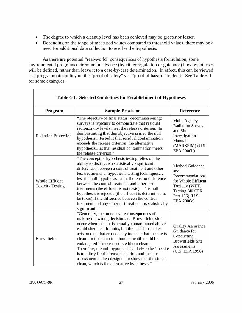
EPA QA/G-9R February 2006 27
• The degree to which a cleanup level has been achieved may be greater or lesser. • Depending on the range of measured values compared to threshold values, there may be a
need for additional data collection to resolve the hypothesis.
As there are potential “real-world” consequences of hypothesis formulation, some environmental programs determine in advance (by either regulation or guidance) how hypotheses will be defined, rather than leave it to a case-by-case determination. In effect, this can be viewed as a programmatic policy on the “proof of safety” vs. “proof of hazard” tradeoff. See Table 6-1 for some examples.
Table 6-1. Selected Guidelines for Establishment of Hypotheses
Program Sample Provision Reference
Radiation Protection
“The objective of final status (decommissioning) surveys is typically to demonstrate that residual radioactivity levels meet the release criterion. In demonstrating that this objective is met, the null hypothesis…tested is that residual contamination exceeds the release criterion; the alternative hypothesis…is that residual contamination meets the release criterion.”
Multi-Agency Radiation Survey and Site Investigation Manual (MARSSIM) (U.S. EPA 2000b)
Whole Effluent Toxicity Testing
“The concept of hypothesis testing relies on the ability to distinguish statistically significant differences between a control treatment and other test treatments….hypothesis testing techniques… test the null hypothesis…that there is no difference between the control treatment and other test treatments (the effluent is not toxic). This null hypothesis is rejected (the effluent is determined to be toxic) if the difference between the control treatment and any other test treatment is statistically significant.”
Method Guidance and Recommendations for Whole Effluent Toxicity (WET) Testing (40 CFR Part 136) (U.S. EPA 2000c)
Brownfields
“Generally, the more severe consequences of making the wrong decision at a Brownfields site occur when the site is actually contaminated above established health limits, but the decision-maker acts on data that erroneously indicate that the site is clean. In this situation, human health could be endangered if reuse occurs without cleanup. Therefore, the null hypothesis is likely to be ‘the site is too dirty for the reuse scenario’, and the site assessment is then designed to show that the site is clean, which is the alternative hypothesis ”
Quality Assurance Guidance for Conducting Brownfields Site Assessments (U.S. EPA 1998)
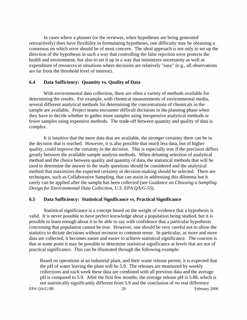
EPA QA/G-9R February 2006 28
In cases where a planner (or the reviewer, when hypotheses are being generated retroactively) does have flexibility in formulating hypotheses, one difficulty may be obtaining a consensus on which error should be of most concern. The ideal approach is not only to set up the direction of the hypothesis in such a way that controlling the false rejection error protects the health and environment, but also to set it up in a way that minimizes uncertainty as well as expenditure of resources in situations where decisions are relatively "easy" (e.g., all observations are far from the threshold level of interest). 6.4 Data Sufficiency: Quantity vs. Quality of Data
With environmental data collection, there are often a variety of methods available for determining the results. For example, with chemical measurements of environmental media, several different analytical methods for determining the concentrations of chemicals in the sample are available. Project teams encounter difficult decisions in the planning phase when they have to decide whether to gather more samples using inexpensive analytical methods or fewer samples using expensive methods. The trade-off between quantity and quality of data is complex.
It is intuitive that the more data that are available, the stronger certainty there can be in
the decision that is reached. However, it is also possible that much less data, but of higher quality, could improve the certainty in the decision. This is especially true if the precision differs greatly between the available sample analysis methods. When debating selection of analytical method and the choice between quality and quantity of data, the statistical methods that will be used to determine the answer to the study questions should be considered and the analytical method that maximizes the expected certainty in decision-making should be selected. There are techniques, such as Collaborative Sampling, that can assist in addressing this dilemma but it rarely can be applied after the sample has been collected (see Guidance on Choosing a Sampling Design for Environmental Data Collection, U.S. EPA QA/G-5S). 6.5 Data Sufficiency: Statistical Significance vs. Practical Significance
Statistical significance is a concept based on the weight of evidence that a hypothesis is valid. It is never possible to have perfect knowledge about a population being studied, but it is possible to learn enough about it to be able to say with confidence that a particular hypothesis concerning that population cannot be true. However, one should be very careful not to allow the statistics to dictate decisions without recourse to common sense. In particular, as more and more data are collected, it becomes easier and easier to achieve statistical significance. The concern is that at some point it may be possible to determine statistical significance at levels that are not of practical significance. This can be illustrated through the following example:
Based on operations at an industrial plant, and their waste release permit, it is expected that the pH of water leaving the plant will be 5.9. The releases are monitored by weekly collections and each week these data are combined with all previous data and the average pH is compared to 5.9. After the first few months, the average release pH is 5.88, which is not statistically significantly different from 5.9 and the conclusion of no real difference

EPA QA/G-9R February 2006 29
justified. After several years have elapsed the average release pH is 5.8996 and this is statistically significantly different from the permitted value of 5.9, but yet a conclusion of a real difference be justified? This is a case where having so much data allows the reviewer to identify very small differences from the expected level, but the statistically significant result may very well not have any practical significance (in this case a difference in pH of 0.0004, which is barely measurable).
While statistics provide a strong and essential tool for environmental decision-making, the science of statistics is not a substitute for common sense and can lead to bad decisions if not tempered with practicality. 6.6 Conclusions This document may be used to either assist in conducting a DQA, or in reviewing an existing DQA. Steps 1-5 should be followed roughly in the order presented. However, it may occasionally be productive to revisit earlier steps based on information gleaned during the DQA process. For that reason it is often beneficial to view this as an iterative process rather than one for which all inputs should be gathered sequentially. Data quality assessment should be conducted on all data intended for use in decision-making, regardless of the level of planning defined prior to data collection. The information contained in this document is meant to provide an overview of the DQA process. There are several levels of assistance available from EPA for those conducting DQAs:
1. The checklist in Appendix F provides a de minimus list of outputs necessary for a complete DQA. This can be used on its own to check that the DQA is complete.
2. This document provides further explanation for each of the outputs on the checklist.
The user can either begin with the checklist and refer back to this document as necessary, or follow the steps as laid out in chapters 1-5 of this document directly.
3. Data Quality Assessment: Statistical Methods for Practitioners (Final Draft) (EPA
QA/G-9S) provides much more detail for implementation of a DQA. Again the DQA reviewer can either refer to that document as necessary for details of implementation of selected methods, or can perform a DQA by following chapters 1-5 of that document directly.
4. EPA Quality Staff offers an introductory course in Data Quality Assessment. If the
course is not being offered at a time and location convenient for you, it may be downloaded from http://www.epa.gov/quality/trcourse.html#intro_dqa.

EPA QA/G-9R February 2006 30

EPA QA/G-9R February 2006 31
REFERENCES U.S. Environmental Protection Agency, 1998. Quality Assurance Guidance for Conducting
Brownfields Site Assessments EPA 540-R-98-038. Office of Solid Waste and Emergency Response
U.S. Environmental Protection Agency, 2000a. Guidance on the Data Quality Objectives Process
(QA/G-4) U.S. Environmental Protection Agency, 2000b. Multi-Agency Radiation Survey and Site
Investigation Manual (MARSSIM) U.S. Environmental Protection Agency, 2000c. Method Guidance and Recommendations for
Whole Effluent Toxicity (WET) Testing (40 CFR Part 136) U.S. Environmental Protection Agency, 2002. Guidance on Choosing a Sampling Design for
Environmental Data Collection (EPA QA/G-5S) U.S. Environmental Protection Agency, 2004. Data Quality Assessment: Statistical Methods for
Practitioners (EPA QA/G-9S) (Final Draft)

EPA QA/G-9R February 2006 32

EPA QA/G-9R February 2006 33
APPENDIX A: COMMONLY USED STATISTICAL QUANTITIES
Measures of Central Tendency: Measures of the center of a sample of data points
Mean: The most commonly used measure of the center of a sample is the sample mean, denoted by X . This estimate of the center of a sample can be thought of as the "center of gravity" of the sample. The sample mean is an arithmetic average for simple sampling designs; however, for complex sampling designs, such as stratification, the sample mean is a weighted arithmetic average. The sample mean is influenced by extreme values (large or small) and non-detects. Median: The sample median is the second most popular measure of the center of the data. This value falls directly in the middle of the data when the measurements are ranked in order from smallest to largest. This means that ½ of the data are smaller than or equal to the sample median and ½ of the data are larger than or equal to the sample median. The median is another name for the 50th percentile. The median is not influenced by extreme values and can easily be used in the case of censored data (non-detects). Mode: The third method of measuring the center of the data is the mode. The sample mode is the value of the sample that occurs with the greatest frequency. Since this value may not always exist, or if it does it may not be unique, this value is the least commonly used. However, the mode is useful for describing qualitative data.
Measures of Relative Standing: Relative position of one observation in relation to all observations
Percentiles: A percentile is the data value that is greater than or equal to a given percentage of the data values. Stated in mathematical terms, the pth percentile is a data value that is greater than or equal to p% of the data values and is less than or equal to (1-p)% of the data values. Therefore, if 'x' is the pth percentile, then p% of the values in the data set are less than or equal to x, and (100-p)% of the values are greater than or equal to x. A sample percentile may fall between a pair of observations. For example, the 75th percentile of a data set of 10 observations is not uniquely defined as it falls between the 7th and 8th largest values. Important percentiles usually reviewed are the quartiles of the data, the 25th, 50th, and 75th percentiles. Also important for environmental data are the 90th, 95th, and 99th percentile where a decision maker would like to be sure that 90%, 95%, or 99% of the contamination levels are below a fixed risk level. There are several methods for computing sample percentiles. Quantiles: A quantile is very similar in concept to a percentile; however, a percentile represents a percentage whereas a quantile represents a fraction. If x is the p/100 quantile of the data, then the fraction p/100 of the data values lie at or below x and the fraction (1-p)/100 of the data values lie at or above x, whereas if 'x' is the pth percentile, then at least p% of the values in the data set lie at or below x, and at least (100-p)% of the values lie at or above x. For example, the 0.95

EPA QA/G-9R February 2006 34
quantile has the property that 0.95 of the observations lie at or below x and 0.05 of the data lie at or above x.
Measures of Dispersion: Measures of how the data spread out from the center
Range: The easiest measure of dispersion to compute is the sample range, maximum - minimum. For small samples, the range is easy to interpret and may adequately represent the dispersion of the data. For large samples, the range is not very informative because it only considers (and therefore is greatly influenced) by extreme values which could be outliers. Variance and Standard Deviation: The variance measures the dispersion of the data from the mean and is denoted by s2. A large variance implies that there is a large spread among the data so that the data are not clustered around the mean. A small variance implies that there is little spread among the data so that most of the data are near the mean. The variance is affected by extreme values and by a large number of non-detects. The standard deviation (s) is the square root of the sample variance and has the same unit of measure as the data. Coefficient of Variation: The coefficient of variation (CV) is a unitless measure that allows the comparison of dispersion across several sets of data. The CV is the standard deviation divided by the mean. It is also called the relative standard deviation (RSD). Interquartile Range: When extreme values are present, the interquartile range may be more representative of the dispersion of the data than the standard deviation. It is the difference between the first and third quartiles (25th and 75th percentiles) of the data. This statistical quantity does not depend on extreme values and is therefore useful when the data include a large number of non-detects.
Measures of Association: The relationship between two or more variables
Pearson’s Correlation Coefficient: The Pearson (often “Pearson” is omitted) correlation coefficient measures a linear relationship between two variables. Values of the correlation coefficient close to +1 (positive correlation) imply that as one variable increases so does the other, the reverse holds for values close to –1 (negative correlation). Values close to 0 imply little correlation between the variables. The correlation coefficient does not detect nonlinear relationships so it should be used only in conjunction with a scatterplot graph of the data. A scatterplot can be used to determine if the correlation coefficient is meaningful or if some measure of nonlinear relationships should be used. The correlation coefficient can be significantly changed by extreme values so a scatter plot should be used first to identify such values. Note that correlation does not imply cause and effect. Spearman’s Rank Correlation Coefficient: An alternative to the Pearson correlation is Spearman’s rank correlation coefficient. It is calculated by first replacing each X value by its rank (i.e., 1 for the smallest X value, 2 for the second smallest, etc.) and each Y value by its rank. These pairs of ranks are then treated as the (X,Y) data and Spearman’s rank correlation is

EPA QA/G-9R February 2006 35
calculated using the same formulae as for Pearson’s correlation. Spearman’s correlation will not be altered by nonlinear increasing transformations of the Xs or the Ys.

EPA QA/G-9R February 2006 36

EPA QA/G-9R February 2006 37
Example Box- and-Whiskers Plot
APPENDIX B: GRAPHICAL REPRESENTATION OF DATA
This appendix contains examples of several types of common graphical representations of data. Histogram/Frequency Plots Description: Divide the data range into units, count the number of points within the units, and display the data as the height (frequency plot) or area (histogram) within a bar graph. Drawbacks: Demands the reviewer make arbitrary choices to partition the data. Uses: Distribution - A normal distribution will be bell-shaped. Symmetry - Symmetric data has the same amount of
data either side of the center point. Variability - Both plots indicate the spread of the data
(standard deviation, variance). Skewness – Right (positive) skewed data have a large
number of low values, relatively few high values. NOTE: The y-axis of a histogram can also represent relative frequencies which are frequencies divided by the sample size. Box- and-Whiskers Plot Description: Composed of a central box divided by a horizontal line representing the median and two lines extending out from the box called whiskers. The length of the central box indicates the spread of the bulk of the data (the central 50%) while the length of the whiskers show how stretched the tails of the distribution are. The sample mean is displayed using a ‘+’ sign and any unusually small or large data points are displayed by a ‘*’ on the plot. Drawbacks: Schematic diagram instead of numerical. Uses: Statistical Quantities - Visualize the relationships.
Symmetry - If the distribution is symmetrical, the box is divided in two equal halves by the median, the whiskers will be the same length and the number of extreme data points will be distributed equally on either end of the plot for symmetric data. Outliers - Values that are unusually large or small are easily identified.
0 5 10 15 20 25 30 35 400
2
4
6
8
10
Concentration (ppm)
Num
ber o
f Obs
erva
tions
0 5 10 15 20 25 30 35 400
2
4
6
8
Concentration (ppm)
Perc
enta
ge o
f Obs
erva
tions
(per
ppm
)Example Frequency Plot
Example Histogram

EPA QA/G-9R February 2006 38
Stem-and-Leaf Plot Description: Each observation in the stem-and-leaf plot consists of two parts: the stem of the observation and the leaf. The stem is usually made up of the leading digit of the numerical values while the leaf is made up of trailing digits in the order that corresponds to the order of magnitude from left to right. The stem is displayed on the vertical axis and the data points displayed from left to right. Advantages: Stores data in a compact form while, at the same time, sorts the data from smallest to largest. Non-detects can be placed in a single stem. Drawbacks: Demands the reviewer make arbitrary choices to partition the data. Uses: Distribution - Normally distributed data is approximately bell shaped.
Symmetry - The top half of the stem-and-leaf plot will be a mirror image of the bottom half of the stem-and-leaf plot for symmetric data. Skewness - Left skewed (negative) data have many high values, relatively few low values. Left skewed data are relatively rare with environmental measurements.
Ranked Data Plot Description: A plot of the data from smallest to largest at evenly spaced intervals. Advantages: Easy to construct, easy to interpret, makes no assumptions about a model for the data, and shows every data point. Uses: Density - A large amount of data values have a
flat slope, i.e., the graph rises slowly. A small amount of data values have a large slope, i.e., the graph rises quickly.
Skewness - A plot of data that are skewed to the right (many low values, but few high) extends mores sharply at the top giving the graph a ‘J’ shape. A plot of data that are skewed to the left (few low values, but many high) increases sharply near the bottom giving the graph an inverted ‘J’ shape.
Symmetry - The top portion of the graph will stretch to upper right corner in the same way the bottom portion of the graph stretches to lower left, creating an S-shape, for symmetric data.
Example Stem-and-Leaf Plot
Dat
a Va
lues
Smallest Largest
Example Ranked Data Plot

EPA QA/G-9R February 2006 39
Quantile Plot Description: A graph of the data against the quantiles. Advantages: Easy to construct, easy to interpret, makes no assumptions about a model for the data, and displays every data point. Uses: Density - A large amount of data values
has a flat slope, i.e., graph rises slowly. A small amount of data values has a large slope, i.e., the graph rises quickly.
Skewness - A plot of data that are skewed to the right (many low values, but few high) is steeper at the top right than the bottom left. A quantile plot of data that are skewed to the left (few low values, but many high) increases sharply near the bottom left of the graph. Symmetry - The top portion of the graph will stretch to the upper right corner in the same way the bottom portion of the graph stretches to the lower left, creating an S-shape for symmetric data.
Normal Probability Plot (Two Variables) Description: The graph of the quantiles of a data set against the quantiles of the normal distribution plotted on normal probability graph paper. Drawbacks: Tedious to generate by hand, but can be created with most statistical software. Uses: Normality - The graph of normally distributed
data should be linear. Symmetry - The degree of symmetry can be
determined by comparing the right and left sides of the plot. Outliers - Data values that are much larger or much smaller than rest will cause the other data values to be compressed into the middle of the graph, ruining the resolution.
0 0.2 0.4 0.6 0.8 10
1
2
3
4
Fraction of Data (f-values)
Dat
a Va
lues Upper
QuartileLowerQuartile
Interquartile Range
Median
Example Quantile Plot
2 5 10 20 30 40 50 60 70 80 90 95 98
10
12
14
16
18
20
0
2
4
6
8
Example Normal Probability Plot

EPA QA/G-9R February 2006 40
Scatterplot (Two Paired Variables) Description: Paired values are plotted on separate axes. Advantages: Clearly shows the relationship between two variables, easy to construct. Uses: Correlation/Trends - Linearly correlated
variables cluster around straight line. Nonlinear patterns may be obvious. Outliers - Potential outliers from a single variable or from paired variables may be identified. Clustering - Points clustered together can be easily identified.
Time Plot (Temporal Data) Description: A plot of the data over time. Advantages: Easy to generate and interpret. Uses: Trends - Including large-scale and small-
scale, seasonal (patterns that repeat over time), and directional (downward/upward trends) including subtle shifts. Serial Correlation – Shows relationship between successive observations.
Variability - Look for increasing or decreasing variability over time.
Outliers - Values that are unusually large or small are easily identified.
0 2 4 6 80
10
20
30
40
Chromium VI (ppb)
PCE
(ppb
)
Example Scatter Plot
Example Time Plot
0 5 10 15 20 25 30 35 40 45 500
5
10
15
20
Time
Dat
a Va
lues

EPA QA/G-9R February 2006 41
Posting Plots (Spatial Data) Description: Map of data locations together
with corresponding data values. Drawback: May not be feasible for a large amount of data Uses: Errors - Identify obvious errors in data location and values.
Sampling Design - Easy way to review design.
Trends - Obvious trends can be identifified.
4.0 11.6 14.9 17.4 17.7 12.4
28.6 7.7 15.2 35.5 14.7 16.5
8.9 14.7 10.9 12.4 22.8 19.1
10.2 5.2 4.9 17.2
Cre
ek
Roa
d
Example Posting Plot

EPA QA/G-9R February 2006 42

EPA QA/G-9R February 2006 43
APPENDIX C: COMMON HYPOTHESIS TESTS
Ran
dom
Sam
ple
Inde
pend
ence
App
roxi
mat
ely
Nor
mal
Dis
tribu
tion
No
Out
liers
No
(or f
ew) N
Ds
Other Assumptions
One-Sample t-Test X X X X X
Wilcoxon Signed Rank Test X X
• Not many data values are identical • Symmetric
Compare a mean to a fixed number - for example, to determine whether the mean contaminant level is greater than 10 ppm
Chen Test X X X • Data come from a right-skewed
distribution (like a lognormal distribution)
Wilcoxon Signed Rank Test X X
• Not many data values are identical • Symmetric
Compare a median to a fixed number - for example, to determine whether the median is greater than 8 ppm Sign Test X X
• Not many sample values equal to the fixed level (reduces efficiency)
Compare a proportion or percentile to a fixed number - for example, to determine if 95% of all companies emitting sulfur dioxide into the air are below a fixed discharge level.
One-Sample Proportion Test X X Not many sample values equal to the
fixed level (reduces efficiency)
Compare a variance to a fixed number - for example, to determine if the variability of an analytical method exceeds a fixed number.
Chi-squared test X X X

EPA QA/G-9R February 2006 44
Ran
dom
Sam
ple
Inde
pend
ence
App
roxi
mat
ely
Nor
mal
Dis
tribu
tion
No
Out
liers
No
(or f
ew) N
Ds
Other Assumptions
Compare a correlation coefficient to a fixed number - for example, determine if the correlation between two contaminants exceeds 0.5.
z-Test of a Correlation Coefficient
X X X X • Linear relationship
Student's Two-Sample t-Test
X X X X • Approximately the same underlying variance for both populations
Compare two means - for example, to compare the mean contaminant level at a remediated Superfund site to a background site or to compare the mean of two different drinking water wells.
Satterthwaite's Two-Sample t-Test
X X X X
Compare several means against a control population - for example, to compare different analytical methods to the standard method.
Dunnett’s Test X X • All group sizes are approximately equal
Compare two proportions or percentiles - for example, to compare the proportion of children with elevated blood lead in one area to the proportion of children with elevated blood lead in another area.
Two-Sample Test for Proportions X X
Compare two correlations - for example, to determine which of two contaminants is a better predictor of a third
Kendall’s Test X X X • Linear relationships

EPA QA/G-9R February 2006 45
Ran
dom
Sam
ple
Inde
pend
ence
App
roxi
mat
ely
Nor
mal
Dis
tribu
tion
No
Out
liers
No
(or f
ew) N
Ds
Other Assumptions
F-Test X X X X X • 2 populations only
Bartlett's Test X X X X X • 2 or more populations Compare the variances of 2 or more populations - for example, to compare the variances of several analytical methods.
Levene's Test X X X X X • 2 or more populations
Wilcoxon Signed Rank Test
X X
• The two distributions have the same shape and dispersion (approximately)
• Only a few identical values • The difference is assumed to be some
fixed amount
Determine if one population distribution differs from another distribution - for example, to compare the contaminant levels at a remediated Superfund site those of a background area. Quantile Test X X X
• Equal variances • Data generated using systematic or
simple random sampling design • The difference is assumed to be only
in the upper part of the distributions

EPA QA/G-9R February 2006 46

EPA QA/G-9R February 2006 47
APPENDIX D: COMMONLY USED STATEMENTS OF HYPOTHESES
Type of Decision Null Hypothesis Alternative Hypothesis
Compare environmental conditions to a fixed threshold value, such as a regulatory standard or acceptable risk level; presume that the true condition is at most the threshold value.
The value of the measured parameter is at most the threshold value.
The value of the measured parameter is greater than the threshold value.
Compare environmental conditions to a fixed threshold value; presume that the true condition is at least the threshold value.
The value of the measured parameter is at least the threshold value.
The value of the measured parameter is less than the threshold value.
Compare environmental conditions to a fixed threshold value; presume that the true condition is equal to the threshold value and the reviewer is concerned whenever conditions vary significantly from this value.
The value of the measured parameter is equal to the threshold value.
The value of the measured parameter is not equal to the threshold value.
Compare environmental conditions associated with two different populations to a fixed threshold value such as a regulatory standard or acceptable risk level; presume that the true condition is at most the threshold value. If it is presumed that conditions associated with the two populations are the same, the threshold value is 0.
The difference between the two measured parameters is at most the threshold value.
The difference between the two measured parameters is greater than the threshold value.
Compare environmental conditions associated with two different populations to a fixed threshold value such as a regulatory standard or acceptable risk level; presume that the true condition is at least the threshold value. If it is presumed that conditions associated with the two populations are the same, the threshold value is 0.
The difference between the two measured parameters is at least the threshold value.
The difference between the two measured parameters is less than the threshold value.
Compare environmental conditions associated with two different populations to a fixed threshold value such as a regulatory standard or acceptable risk level; presume that the true condition is equal to the threshold value. If it is presumed that conditions associated with the two populations are the same, the threshold value is 0.
The difference between the two measured parameters is equal to the threshold value.
The difference between the two measured parameters is not equal to the threshold value.

EPA QA/G-9R February 2006 48

EPA QA/G-9R February 2006 49
APPENDIX E: COMMON ASSUMPTIONS AND TRANSFORMATIONS Independence
The assumption of independence of data is the key to the validity of the false rejection and false acceptance error rates associated with a selected statistical test. Environmental data are particularly susceptible to correlation problems due to the fact that data are collected under a spatial pattern (for example a grid) or sequentially over time (for example, daily readings from a monitoring station). Readings taken close together can be correlated (known as autocorrelation) and the effectiveness of statistical tests is diminished. When data are truly independent between themselves, the correlation between data points is by definition zero and statistical tests have the desired chosen decision error rates (given appropriate other assumptions have been satisfied).
The reason non-independence is an issue for statistical testing situations is that if
observations are positively correlated over time or space, then the effective sample size for a test tends to be smaller than the actual sample size – i.e., each additional observation does not provide as much "new" information because its value is partially determined by (or a function of) the value of adjacent observations. This smaller effective sample size means that the degrees of freedom for the test statistic decreases, or equivalently, the test is not as powerful as originally thought. In addition to affecting the false acceptance error rate, applying the usual tests to correlated data tends to result in a test whose actual significance level (false rejection error rate) is larger than the nominal error rate.
Non-independence also occurs when data are actually collected in groups and not
randomly over the entire sample. For example, suppose there are 5 locations each with 4 measurements on a contaminant. This is different from 20 locations each with 1 measurement on a contaminant. If the 5-location data are analyzed as if it was 20-location data incorrect conclusions may occur. In the 5-location data set, each group of 4 measurements could be expected to be approximately the same and, overall, not as diverse as the 20-location data set. In statistical terms, this is because the 5-location data set variability can be partitioned into two sources of variability: between locations, and within locations. The 20-location data set cannot be partitioned into the two sources as only 1 measurement was taken at each location. Between locations variability is usually much larger than within location variability and so the 5-location data can be considered “more lumpy” than the 20-location data and this will affect the analysis.
One of the most effective ways to determine statistical independence for data collected
over time is through use of the Rank von Neumann Test. Compared to other tests of statistical independence, the rank von Neumann test has been shown to be more powerful over a wide variety of cases. This means that very little effectiveness is lost by always using the ranks in place of the original concentrations; the rank von Neumann ration should still correctly detect non-independent data. Details on how to use the rank von Neumann test are to be found in Data Quality Assessment: Statistical Methods for Practitioners (Final Draft) (EPA QA/G-9S).
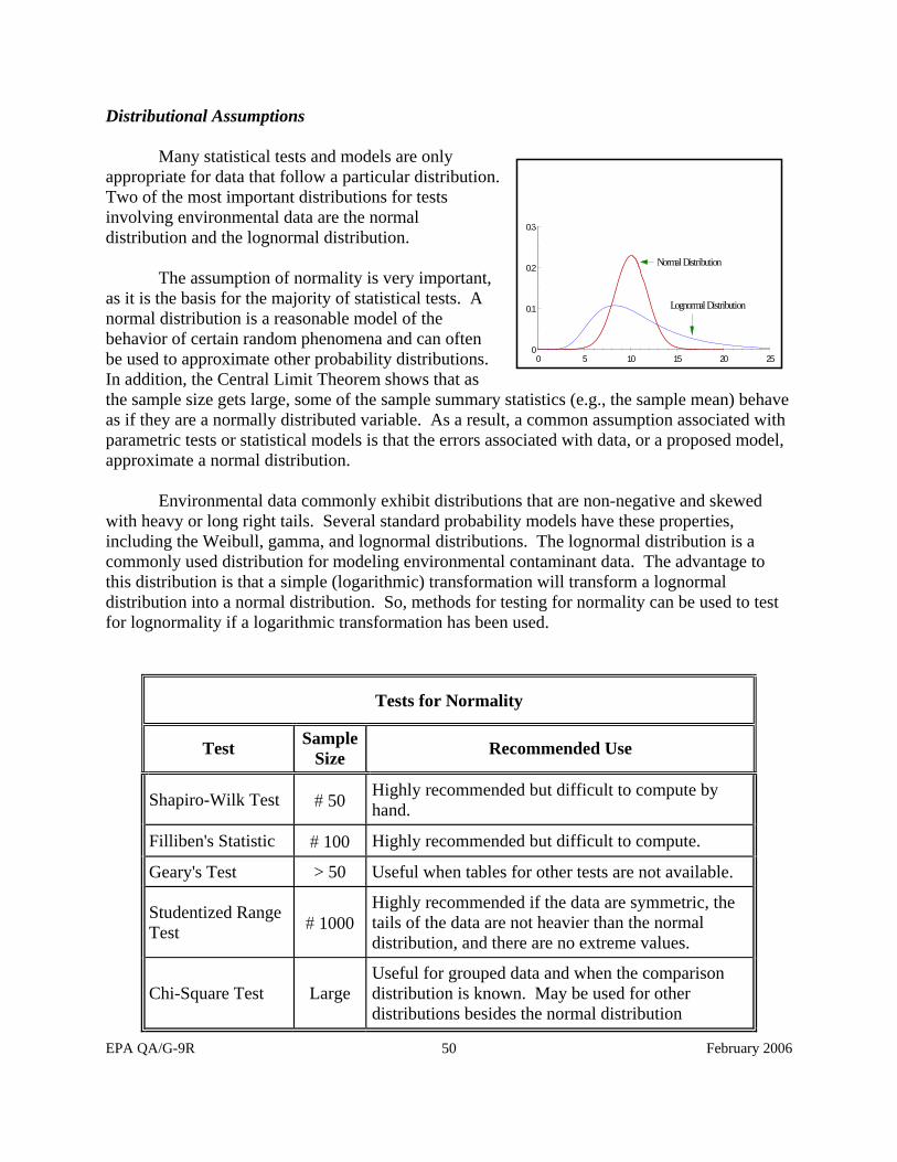
EPA QA/G-9R February 2006 50
Distributional Assumptions
Many statistical tests and models are only appropriate for data that follow a particular distribution. Two of the most important distributions for tests involving environmental data are the normal distribution and the lognormal distribution.
The assumption of normality is very important,
as it is the basis for the majority of statistical tests. A normal distribution is a reasonable model of the behavior of certain random phenomena and can often be used to approximate other probability distributions. In addition, the Central Limit Theorem shows that as the sample size gets large, some of the sample summary statistics (e.g., the sample mean) behave as if they are a normally distributed variable. As a result, a common assumption associated with parametric tests or statistical models is that the errors associated with data, or a proposed model, approximate a normal distribution.
Environmental data commonly exhibit distributions that are non-negative and skewed with heavy or long right tails. Several standard probability models have these properties, including the Weibull, gamma, and lognormal distributions. The lognormal distribution is a commonly used distribution for modeling environmental contaminant data. The advantage to this distribution is that a simple (logarithmic) transformation will transform a lognormal distribution into a normal distribution. So, methods for testing for normality can be used to test for lognormality if a logarithmic transformation has been used.
Tests for Normality
Test Sample Size Recommended Use
Shapiro-Wilk Test # 50 Highly recommended but difficult to compute by hand.
Filliben's Statistic # 100 Highly recommended but difficult to compute.
Geary's Test > 50 Useful when tables for other tests are not available.
Studentized Range Test # 1000
Highly recommended if the data are symmetric, the tails of the data are not heavier than the normal distribution, and there are no extreme values.
Chi-Square Test Large Useful for grouped data and when the comparison distribution is known. May be used for other distributions besides the normal distribution
0 5 10 15 20 250
0.1
0.2
0.3
0.4
Lognormal Distribution
Normal Distribution

EPA QA/G-9R February 2006 51
Outliers
Outliers are measurements that are extremely large or small relative to the rest of the data and, therefore, are suspected of misrepresenting the population from which they were collected. Outliers may result from transcription errors, data-coding errors, or measurement system problems such as instrument breakdown. However, outliers may also represent true extreme values of a distribution (for instance, hot spots) and indicate more variability in the population than was expected. Not removing true outliers and removing false outliers both lead to a distortion of estimates of population parameters.
Statistical outlier tests give the reviewer probabilistic evidence that an extreme value
(potential outlier) does not "fit" with the distribution of the remainder of the data and is therefore a statistical outlier. These tests should only be used to identify data points that need further investigation. The tests alone cannot determine whether a statistical outlier should be discarded or corrected within a data set; this decision should be based on expert or scientific grounds.
Potential outliers may be identified through a graphical representation of the data. If a
data point is found to be an outlier, the reviewer may either: 1) correct the data point; 2) discard the data point from analysis; or 3) use the data point in all analyses. This decision should be based on scientific reasoning in addition to the results of the statistical test. One should never discard an outlier based solely on a statistical test. Instead, the decision to discard an outlier should be based on some scientific or quality assurance basis. Discarding an outlier from a data set should be done with extreme caution, particularly for environmental data sets, which often contain legitimate extreme values. If an outlier is discarded from the data set, all statistical analysis of the data should be applied to both the full and truncated data set so that the effect of discarding observations may be assessed. If scientific reasoning does not explain the outlier, it should not be discarded from the data set.
If no data points are discarded, document the identification of any "statistical" outliers by
documenting the statistical test performed and the possible scientific reasons investigated. If any data points are discarded, document each data point, the statistical test performed, the scientific reason for discarding each data point, and the effect on the analysis of deleting the data points.
Statistical Tests for Outliers
Sample Size Test Assumes Normality
Multiple Outliers
n # 25 Extreme Value Test Yes Yes
n # 50 Discordance Test Yes No
n ∃ 25 Rosner's Test Yes Yes
n ∃ 50 Walsh's Test No Yes
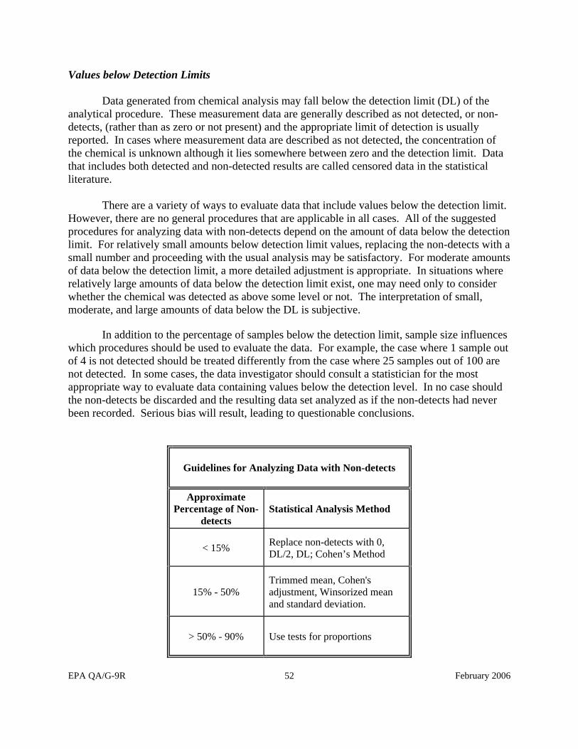
EPA QA/G-9R February 2006 52
Values below Detection Limits Data generated from chemical analysis may fall below the detection limit (DL) of the
analytical procedure. These measurement data are generally described as not detected, or non-detects, (rather than as zero or not present) and the appropriate limit of detection is usually reported. In cases where measurement data are described as not detected, the concentration of the chemical is unknown although it lies somewhere between zero and the detection limit. Data that includes both detected and non-detected results are called censored data in the statistical literature.
There are a variety of ways to evaluate data that include values below the detection limit.
However, there are no general procedures that are applicable in all cases. All of the suggested procedures for analyzing data with non-detects depend on the amount of data below the detection limit. For relatively small amounts below detection limit values, replacing the non-detects with a small number and proceeding with the usual analysis may be satisfactory. For moderate amounts of data below the detection limit, a more detailed adjustment is appropriate. In situations where relatively large amounts of data below the detection limit exist, one may need only to consider whether the chemical was detected as above some level or not. The interpretation of small, moderate, and large amounts of data below the DL is subjective.
In addition to the percentage of samples below the detection limit, sample size influences
which procedures should be used to evaluate the data. For example, the case where 1 sample out of 4 is not detected should be treated differently from the case where 25 samples out of 100 are not detected. In some cases, the data investigator should consult a statistician for the most appropriate way to evaluate data containing values below the detection level. In no case should the non-detects be discarded and the resulting data set analyzed as if the non-detects had never been recorded. Serious bias will result, leading to questionable conclusions.
Guidelines for Analyzing Data with Non-detects
Approximate Percentage of Non-
detects Statistical Analysis Method
< 15% Replace non-detects with 0, DL/2, DL; Cohen’s Method
15% - 50% Trimmed mean, Cohen's adjustment, Winsorized mean and standard deviation.
> 50% - 90% Use tests for proportions

EPA QA/G-9R February 2006 53
Transformations Data that do not satisfy statistical assumptions can sometimes be converted or
transformed mathematically into a form that allows standard statistical tests to perform adequately. Any mathematical function that is applied to every point in a data set is called a transformation and the most commonly used transformation is:
Logarithmic (Log X or Ln X): This transformation may be used when the original measurement data follow a lognormal distribution or when the standard deviation of measurements is proportional to the mean of the data points at that level. By transforming the data, assumptions that are not satisfied in the original data can be
satisfied by the transformed data. For instance, a right-skewed distribution can be transformed to be approximately Gaussian (normal) by using a logarithmic or square-root transformation. Then the normal-theory procedures can be applied to the transformed data. If data are lognormally distributed, then apply procedures to logarithms of the data. However, selecting the correct transformation may be difficult and the reviewer should consult a statistician.
Once the data have been transformed, all statistical analysis should be performed on the
transformed data. Very rarely should data be transformed back to the original units after analysis and conclusions drawn with the transformed data set this can lead to biased estimates. For example, estimating quantities such as means, variances, confidence limits, and regression coefficients in the transformed scale typically leads to biased estimates when transformed back into original scale. However, it may be difficult to understand or apply results of statistical analysis expressed in the transformed scale. Therefore, if the transformed data do not give noticeable benefits to the analysis, it is usually better to use the original data with a different technique of analysis.

EPA QA/G-9R February 2006 54

EPA QA/G-9R February 2006 55
APPENDIX F: CHECKLIST OF OUTPUTS FOR DATA QUALITY ASSESSMENT
Step Input G-9R Section
G-9S Section
1 Well-defined project objectives and criteria 1.1 1.1
1 Verification that the hypothesis chosen is consistent with the objective and criteria
1.2 1.1
1 A list of any deviations from the planned sampling design and the effects of these deviations
1.4 1.1
2 Statistics of interest have been calculated 2.2 2.2
2 Graphs and plots of the data are available 2.3 2.3
3 The statistical method for data analysis has been selected 3.0 3.1
3 The assumptions underlying the method have been identified 3.0 3.2 – 3.4
4 Documentation of the method used to verify each assumption and the results from these investigations
4.1 4.1
4 A description and rationale for any corrective actions that were taken, if any were necessary
4.2 & 4.3 4.1
5 Statistical results with a specified significance level 5.1 5.2
5 An assessment of the performance of the sampling design 5.5 5.4
5, 6 Interpretation of the statistical result and study conclusions
5.3 – 5.4, 6.1 & 6.2 5.5
6 A final product or decision 6.3 – 6.5 5.5
G-9R: Data Quality Assessment: A Reviewer’s Guide G-9S: Data Quality Assessment: Statistical Methods for Practitioners (Final Draft)