enzymaticsynthesisofampicillin:nonlinearmodeling...

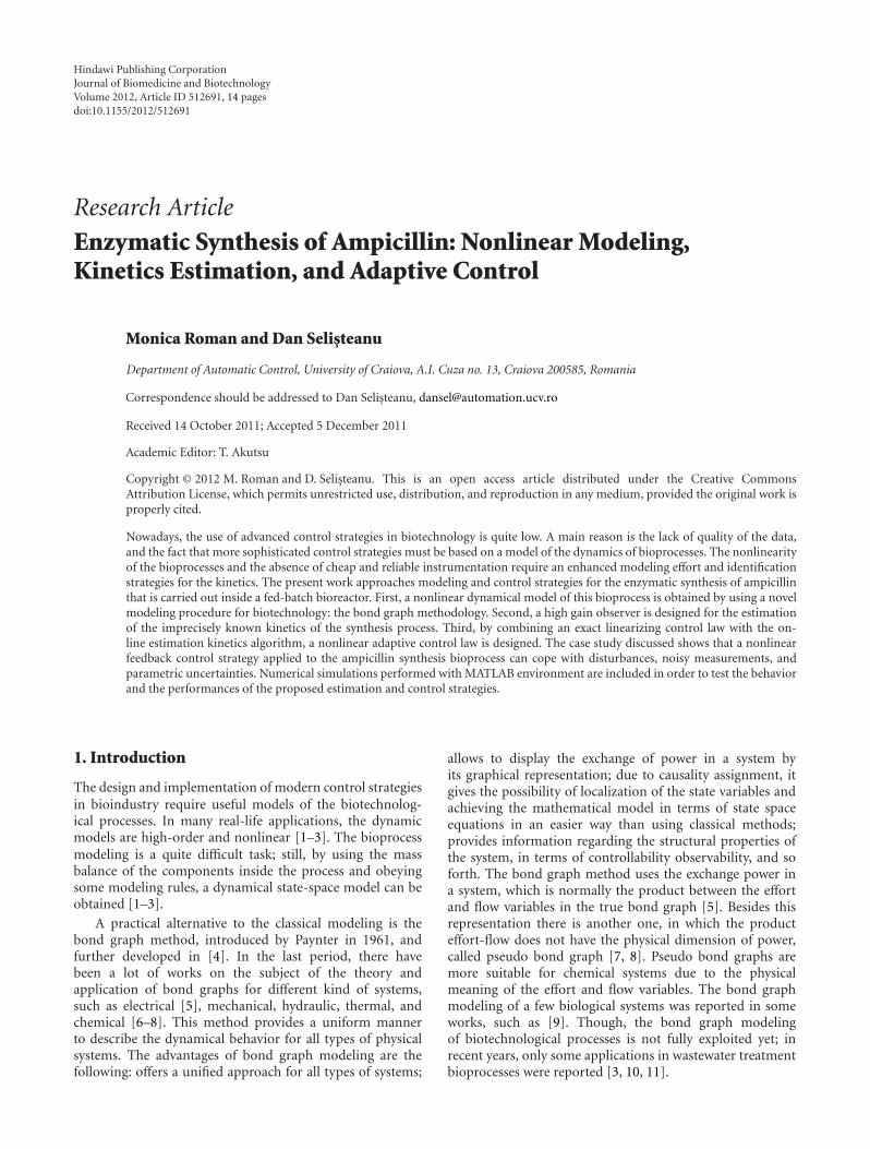
Hindawi Publishing CorporationJournal of Biomedicine and BiotechnologyVolume 2012, Article ID 512691, 14 pagesdoi:10.1155/2012/512691

Research Article

Enzymatic Synthesis of Ampicillin: Nonlinear Modeling,Kinetics Estimation, and Adaptive Control

Monica Roman and Dan Selisteanu

Department of Automatic Control, University of Craiova, A.I. Cuza no. 13, Craiova 200585, Romania

Correspondence should be addressed to Dan Selisteanu, [email protected]

Received 14 October 2011; Accepted 5 December 2011

Academic Editor: T. Akutsu

Copyright © 2012 M. Roman and D. Selisteanu. This is an open access article distributed under the Creative CommonsAttribution License, which permits unrestricted use, distribution, and reproduction in any medium, provided the original work isproperly cited.

Nowadays, the use of advanced control strategies in biotechnology is quite low. A main reason is the lack of quality of the data,and the fact that more sophisticated control strategies must be based on a model of the dynamics of bioprocesses. The nonlinearityof the bioprocesses and the absence of cheap and reliable instrumentation require an enhanced modeling effort and identificationstrategies for the kinetics. The present work approaches modeling and control strategies for the enzymatic synthesis of ampicillinthat is carried out inside a fed-batch bioreactor. First, a nonlinear dynamical model of this bioprocess is obtained by using a novelmodeling procedure for biotechnology: the bond graph methodology. Second, a high gain observer is designed for the estimationof the imprecisely known kinetics of the synthesis process. Third, by combining an exact linearizing control law with the on-line estimation kinetics algorithm, a nonlinear adaptive control law is designed. The case study discussed shows that a nonlinearfeedback control strategy applied to the ampicillin synthesis bioprocess can cope with disturbances, noisy measurements, andparametric uncertainties. Numerical simulations performed with MATLAB environment are included in order to test the behaviorand the performances of the proposed estimation and control strategies.

1. Introduction

The design and implementation of modern control strategiesin bioindustry require useful models of the biotechnolog-ical processes. In many real-life applications, the dynamicmodels are high-order and nonlinear [1–3]. The bioprocessmodeling is a quite difficult task; still, by using the massbalance of the components inside the process and obeyingsome modeling rules, a dynamical state-space model can beobtained [1–3].

A practical alternative to the classical modeling is thebond graph method, introduced by Paynter in 1961, andfurther developed in [4]. In the last period, there havebeen a lot of works on the subject of the theory andapplication of bond graphs for different kind of systems,such as electrical [5], mechanical, hydraulic, thermal, andchemical [6–8]. This method provides a uniform mannerto describe the dynamical behavior for all types of physicalsystems. The advantages of bond graph modeling are thefollowing: offers a unified approach for all types of systems;

allows to display the exchange of power in a system byits graphical representation; due to causality assignment, itgives the possibility of localization of the state variables andachieving the mathematical model in terms of state spaceequations in an easier way than using classical methods;provides information regarding the structural properties ofthe system, in terms of controllability observability, and soforth. The bond graph method uses the exchange power ina system, which is normally the product between the effortand flow variables in the true bond graph [5]. Besides thisrepresentation there is another one, in which the producteffort-flow does not have the physical dimension of power,called pseudo bond graph [7, 8]. Pseudo bond graphs aremore suitable for chemical systems due to the physicalmeaning of the effort and flow variables. The bond graphmodeling of a few biological systems was reported in someworks, such as [9]. Though, the bond graph modelingof biotechnological processes is not fully exploited yet; inrecent years, only some applications in wastewater treatmentbioprocesses were reported [3, 10, 11].

2 Journal of Biomedicine and Biotechnology

To obtain the model of a bioprocess it is necessary toknow the fundaments of the bioprocess and to have goodknowledge concerning the bond graph methodology. Evenif for a bioreactor specialist seems to be easily to obtain themodel via classical method, the bond graph approach can beapplied without difficulty after a short training. The majoradvantage of the proposed approach is that the obtainedbond graph models of the bioprocesses can be easily used andextended to other bioprocesses. For example, the bond graphmodels can be used in order to obtain complex models ofinterconnected bioprocesses [11], and for the direct designof some observers and controllers [12].

The use of modern control techniques for bioprocessesis hampered by the nonlinearity of this kind of processesand the unavailability of several on-line measurements [2].Serious problems appear in the measurement of biologicalvariables, that is, the substrates, biomass and product con-centrations, and so forth. In many cases, the state variables(concentrations) are analyzed manually and as a result thereis not on-line (and real-time) control. These various issuescan be solved using “software sensors.” A software sensor isa combination between a hardware sensor and a softwareestimator. These software sensors can be used not onlyfor the estimation of the concentrations (state variables),but also for the estimation of the kinetic parameters.Very important is the estimation of kinetic rates inside abioreactor, that is, the so-called kinetics of the bioprocess.The growing interest for development of software sensorsfor bioprocess and biological systems is proven by thenumerous publications and applications in this field [1–3, 13–16]. One of the first approaches from historicallypoint of view is based on Kalman filter which leads tocomplex nonlinear algorithms. Another classical techniqueis the Bastin and Dochain approach based on adaptivesystems theory [1]. This strategy consists in the estimationof unmeasured state with asymptotic observers, and afterthat, the measurements and the estimates of state variablesare used for on-line estimation of kinetic rates. This methodis useful, but in some cases, when many reactions areinvolved, the implementation requires the calibration of toomany parameters. For instance, if we have n components’concentrations used for the estimation of m kinetic rates,it is necessary to calibrate 2n tuning parameters [1]. Inorder to overcome this problem, a possibility is to designan estimator using a high gain approach (see [13, 14]). Thegain expression of the high gain observers involves a singletuning parameter whatever the number of components andreactions. High gain observers have evolved over the pasttwo decades as an important tool for the design of outputfeedback control of nonlinear systems [17]. The early workon high gain observers appeared in the late 1980s, andafterwards the technique was developed independently bytwo schools of researchers: a French school lead by Gauthier,Hammouri, Farza, and others, [13, 14], and a US school leadby Khalil [17].

The modeling techniques and the estimation strategieswere used for the design of several control strategies, suchas optimal control [1], sliding mode control [18], adaptivecontrol [1, 18], vibrational control, model predictive control

[19], fuzzy and neural strategies, and so on. Generally speak-ing, due to specificity and nonlinearity of bioprocesses,there is no universal solution to the control problem, andgood solutions are given only by studying each particularbioprocess.

In this paper, which is an extended work of [20], threemain correlated issues concerning the enzymatic bioprocessof ampicillin are studied: modeling, kinetics estimation, andcontrol. First, a pseudo bond graph approach is proposed forthe modeling of an enzymatic synthesis of ampicillin, widelyused in bioindustry. Ampicillin (6-[2-amino-2-phenylacet-amide] penicillanic acid) is a semisynthetic β-lactamic anti-biotic which is very stable at acidic conditions, well absorbedand effective against a wide variety of microorganisms, withlow minimal inhibitory concentration [21–24]. Currently, itis manufactured in bioindustry through a chemical route.These reactions typically involve costly steps, such as verylow temperatures and the use of toxic organic solvents likemethylene chloride and silylation reagents. Enzymatic syn-thesis is an alternative process; it has high selectivity,specificity, and activity in mild reaction conditions (aqueousmedium, neutral pH, and moderate temperatures) [25–27].The main aim of enzyme immobilization is the industrialreuse of enzymes for many reaction cycles [25, 28, 29].Thus, simplicity and improvement of enzyme propertieshave to be strongly associated with the design of protocolsfor enzyme immobilization. A critical review of enzymeimmobilization was presented in [25]. Concerning the useof enzymatic methods in production of semisynthetic β-lactamic antibiotics, several drawbacks and perspectives arepresented by Volpato et al. [30]. These antibacteria agentsare produced in hundreds tons/year scale. They are usuallyproduced by the hydrolysis of natural antibiotics (penicillinG or cephalosporin C). Due to the contaminant reagentsused in conventional chemical route, as well as the highenergetic consumption, biocatalytic approaches have beenstudied for both steps in the production of these veryinteresting medicaments during the last decades [30]. Thehydrolysis of penicillin G to produce 6-APA catalyzed bypenicillin G acylase is one of the most successful examplesof the enzymatic biocatalysis. The dynamical model ofthis complex bioprocess is obtained via the bond graphmethodology by using the reaction scheme and the analysisof biochemical phenomena inside the bioreactor.

Second, because the kinetic rates of the enzymaticbioprocess of ampicillin production are nonlinear and highlyuncertain, an on-line estimation strategy is designed. Someestimation strategies were proposed in the last years, suchas observer-based estimators and the second-order observers(see, e.g., [31]). In this paper, the design and implementationof high gain observers is proposed, with certain advantagesconcerning the robustness against disturbances and thesimple tuning. The high gain estimation scheme does notrequire any model for the kinetic rates. The tuning of theproposed observers is reduced to the calibration of a singleparameter. The nonlinear observer design is based on thework of Gauthier et al. [14], Farza et al. [13], focused onderiving global results under global Lipschitz conditions.

Journal of Biomedicine and Biotechnology 3

Third, an adaptive control law for the enzymatic fed-batch bioprocess of ampicillin production is developed.For bioprocesses taking place into fed-batch reactors, theadaptive control approach is a viable alternative of theoptimal control [1, 2]. In order to design a control law,the so-called exact linearizing approach is used [32]. Thenonlinear controller thus obtained is combined with the highgain estimator for the unknown kinetics, and consequentlyan adaptive controller is obtained. Due to the fact that theimplementation of highgain observer and of the adaptivecontroller requires on-line state estimates, these will beprovided by an asymptotic observer. The performances andthe behavior of the estimation and control algorithms arestudied by using extensive numerical simulations. All thesesimulations are achieved by using the development, pro-gramming and simulation environment Matlab (registeredtrademark of The MathWorks, Inc., USA).

The results obtained in this study show a good behaviorof the adaptive controlled ampicillin synthesis bioprocess.The proposed adaptive control scheme is quite simple,because only two tuning parameters were used, one forestimator and one for the linearizing controller. The bondgraph modeling, estimation, and control strategies can bealso applied to other processes belonging to the nonlinearclass of bioprocesses considered in the study.

2. Materials and Methods

2.1. Bond Graph Modeling Method for the Enzymatic Synthesisof Ampicillin. The bioprocesses are highly complex processesthat take place inside biochemical reactors (bioreactors).The bioreactors can operate in three modes: the continuousmode, the fed-batch mode, and the batch mode [1–3]. A Fed-Batch Bioreactor (FBB) initially contains a small amount ofsubstrates (the nutrients) and microorganisms and is pro-gressively filled with the influent substrates. When the FBB isfull, the content is harvested. A Batch Bioreactor is filled withthe reactant mixture: substrates and microorganisms andallows for a particular time period for the reactions insidethe reactor; after some time the products are removed fromthe tank. In a Continuous Stirred Tank Bioreactor (CSTB),the substrates are fed to the bioreactor continuously andan effluent stream is continuously withdrawn such that theculture volume is constant.

Next, the bond graph method is used in order to obtainthe model of the enzymatic synthesis of ampicillin process,which takes place inside an FBB. Firstly, after a shortpresentation of the bond graph method, a simple prototypefed-batch bioprocess is modeled. After that, the enzymaticsynthesis of ampicillin is widely studied, and the bond graphmodel is obtained by using the reaction scheme, the analysisof the phenomena inside the bioprocess and the bond graphmodeling rules.

Bond graph technique uses the effort-flow analogy todescribe physical processes. A bond graph consists of sub-systems linked together by lines representing power bonds.Each process is described by a pair of variables, effort eand flow f, and their product is the power. The direction ofpower is depicted by a half-arrow. In a dynamic system the

effort and the flow variables, and hence the power fluctuatein time. One of the advantages of bond graph methodis that models of various systems belonging to differentengineering domains can be expressed using a set of onlynine elements. A classification of bond graph elements canbe made up by the number of ports; ports are places whereinteractions with other processes take place. There are oneport elements represented by inertial elements (I), capacitiveelements (C), resistive elements (R), effort sources (Se),and flow sources (Sf ), two ports elements represented bytransformer elements (TF) and gyrator elements (GY), andmultiport elements effort junctions (J0), and flow junctions(J1). I, C, and R elements are passive elements becausethey convert the supplied energy into stored or dissipatedenergy. Se and Sf elements are active elements because theysupply power to the system and TF, GY, 0-and 1-junctionsare junction elements that serve to connect I, C, R, Se,and Sf, and constitute the junction structure of the bondgraph model. Besides the power variables, two other types ofvariables are very important in describing dynamic systemsand these variables, sometimes called energy variables, arethe generalized momentum p as time integral of effort andthe generalized displacement q as time integral of flow [4].

In biotechnology, pseudo bond graph models are accom-plished starting with processes reactions schemes and usingboth base bond graph elements and pseudo bonds with effortand flow variables as concentrations and mass flows. Oneof the simplest biological reactions is the microorganismsgrowth process, with the reaction scheme [1] given by:

Sϕ−→ X , (1)

where S is the substrate,X is the biomass and ϕ is the reactionrate.

This simple growth reaction represents in fact a proto-type reaction, which can be found in almost every biopro-cess. The dynamics of the concentrations of the componentsfrom reaction scheme (1) can be modeled considering themass balance of the components. The dynamical model ofprocess (1) is simple, but if the reaction scheme is morecomplicated, the achievement of the dynamical model isdifficult. In order to model bioprocesses, pseudo bond graphmethod is more appropriate because of the meaning ofvariables involved—effort (concentration) and flow (massflow). From the reaction scheme (1) and taking into accountthe mass transfer through the FBB, using the bond graphmodeling characteristics, the pseudo bond graph modelof the fed-batch bioprocess is achieved see Figure 1. Thebond graph model is depicted in the 20 sim environment(registered trademark of Controllab Products B.V. Enschede,The Netherlands).

The directions of half arrows correspond to the run ofthe reaction, going out from the substrate S towards biomassX . In the bond graph model, the mass balances of thespecies involved in the bioreactor are represented by two 0-junctions: 01,2,3,4 (mass balance for the substrate S) and 07,8,9

(mass balance for the biomass X). Due to the fact that theform of kinetics is complex, nonlinear, and in many casesunknown, the modeling of the reaction kinetics is a difficult


task. A general assumption [1] is that a reaction can takeplace only if all reactants are presented in the bioreactor.Therefore, the reaction rates are necessarily zero wheneverthe concentration of one of the reactants is zero.

In order to model the reaction rate ϕ, because of thedependency of substrate and biomass concentrations, wehave used a modulated two port R element, denoted MR5,6.Mass flow of the component entering the reaction is modeledusing a modulated source flow element Sf 1 and quantitiesexiting from the reaction are modeled using modulatedflow sources elements Sf represented by bonds 3 and 9.This approach was imposed by the dependency of theseelements on Fin: the input feed rate, and on V : volume ofthe bioreactor.

From Sf constitutive equations we have f3 = e3S f3,f9 = e9S f9. The accumulations of substrate and biomass inFBB are represented by bonds 2 and 8 and are modeled usingcapacitive elements C, with the constitutive equations:

e2 = q2

C2=(∫

t

(f1 − f3 − f4

)dt)

C2, (2)

e8 = q8

C8=(∫

t

(f7 − f9

)dt)

C8. (3)

By using the constitutive relations of transformer ele-ments TF4,5 and TF6,7, the relations for flows f4 and f7 areobtained: f4 = k4,5 f5, f7 = f5/k6,7, with k4,5 and k6,7 thetransformers modulus, which are in fact yield coefficientsof the bioprocess (their values equal one for this fed-batchbioprocess). In fact, e2 is the substrate concentration, whichwill be denoted with S, e8 is the biomass concentration X , f5is proportional to ϕ and V , C2 = C8 = V with S f3 = S f9 =Fin. Therefore, from (2) and (3) we will obtain the dynamicalmodel of the fed-batch bioprocess:

VdS

dt= V · S(t) = FinSin − F0S− ϕV ,

VdX

dt= V · X(t) = −F0X + ϕV ,

dV

dt= V(t) = Fin.

(4)

The model (4) expresses the equations of mass balancefor the reaction scheme (1). Taking into account that thedilution rate D = Fin/V , the dynamical behavior of theconcentrations can be easily obtained from (4):

S(t) = DSin −DS− ϕ,

X(t) = −DX + ϕ,

V(t) = Fin.

(5)

Next, this bond graph procedure is extended to themodeling of the enzymatic synthesis of ampicillin takingplace inside a fed-batch bioprocess. Ampicillin (6-[2-amino-2-phenylacetamide] penicillanic acid) is a semisynthetic β-lactamic antibiotic which is very stable at acidic conditions,

0

C:S

TF MR TF

C:X

0Sf

Sf Sf

12

34 5 6 7

8

9

Fin, V

Figure 1: Pseudo bond graph model of the fed-batch prototypebioprocess. The directions of half arrows correspond to the run ofthe reaction, from the substrate S towards biomass X . The massbalances are represented by two 0-junctions: 01,2,3,4 (for S), and 07,8,9

(for X). Mass flows of entering/exiting components are modeledusing modulated source flows Sf. The reaction rate is modeled bya modulated two port R element, denoted MR5,6. Fin is the inputfeed rate (l/h) and V the bioreactor volume (l).

well absorbed and effective against a wide variety of microor-ganisms, with low minimal inhibitory concentration [21–24]. Currently, it is manufactured in bioindustry througha chemical route. For instance, an amino β-lactam, such as6-aminopenicilanic acid (6-APA), having its carboxyl groupprotected, reacts with an activated side-chain derivative (D-phenylglycine acid chloride, to produce ampicillin). Theprotecting group is than removed by hydrolysis. Thesereactions typically involve costly steps, such as very low tem-peratures and the use of toxic organic solvents like methylenechloride and silylation reagents [22]. Enzymatic synthesisis an alternative process; it has high selectivity, specificity,and activity in mild reaction conditions (aqueous medium,neutral pH and moderate temperatures). The influence of thesubstrate structure on the catalytic properties of penicillin Gacylase (PGA) from Escherichia coli in kinetically controlledacylations has been studied in [27]. In particular, the affinityof different β-lactam nuclei towards the active site has beenevaluated considering the ratio between the rate of synthesisand the rate of hydrolysis of the acylating ester. It hasbeen shown that this approach presents several advantagescompared with the classical chemical processes [27].

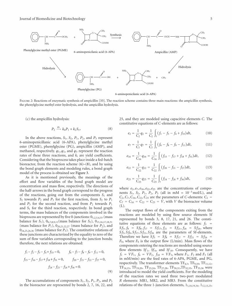
Still, none of the known enzymatic methods have yetbeen upscaled to industrial applicability, due to the highcosts caused by a low yield. Penicillin G acylase (PGA), forexample, can act as a hydrolase as well as a transferase,which means that the same enzyme catalyzes the synthesis ofampicillin as well as the hydrolysis of the activated acyl donorand the hydrolysis of the newly formed antibiotic. The mainreactions involved in the enzymatic synthesis of ampicillinare presented in Figure 2 [33, 34].

The reaction scheme of this complex bioprocess containsthree reactions [31]:

(a) the ampicillin synthesis:

k1S1 + S2ϕ1−→ k5P2 + k6P3, (6)

(b) the phenylglycine methyl ester hydrolysis:

S2ϕ2−→ k3P1 + k7P3, (7)


Ampicillin (AMP)

6-aminopenicilanic acid (6-APA)

Phenylglycine (PG)

6-aminopenicilanic acid (6-APA)Phenylglycine methyl ester (PGME)

CH C

O

O

S

NCOOH

HidrolysisHidrolysis

Synthesis+

+ +

CH3

CH3

CH3

NH3

NH2

OCH3

CH C

O

O

S

NCOOH

CH3

CH3

NH3

NH2

OH

CH C

O

O

S

NCOOH

CH3

CH3

NH3

NHOCH

Figure 2: Reactions of enzymatic synthesis of ampicillin [33]. The reaction scheme contains three main reactions: the ampicillin synthesis,the phenylglycine methyl ester hydrolysis, and the ampicillin hydrolysis.

(c) the ampicillin hydrolysis:

P2ϕ3−→ k4P1 + k2S1, (8)

In the above reactions, S1, S2, P1, P2, and P3 represent6-aminopenicillanic acid (6-APA), phenylglycine methylester (PGME), phenylglycine (PG), ampicillin (AMP), andmethanol, respectively. ϕ1,ϕ2, and ϕ3 represent the reactionrates of these three reactions, and ki are yield coefficients.Considering that the bioprocess takes place inside a fed-batchbioreactor, from the reaction scheme (6)–(8), and by usingthe bond graph elements and modeling rules, a bond graphmodel of the process is obtained see Figure 3.

As it is mentioned previously, the meanings of theeffort and flow variables of the bond graph model areconcentration and mass flow, respectively. The directions ofthe half-arrows in the bond graph correspond to the progressof the reactions, going out from the components S1 andS2 towards P2 and P3 for the first reaction, from S2 to P1

and P3 for the second reaction, and from P2 towards P1

and S1 for the third reaction, respectively. In bond graphterms, the mass balances of the components involved in thebioprocess are represented by five 0-junctions: 01,2,3,4,33 (massbalance for S1), 06,7,8,9,11(mass balance for S2), 015,16,17,18,31

(mass balance for P1), 020,21,22,27 (mass balance for P2), and024,25,26,36 (mass balance for P3). The constitutive relations ofthese junctions are characterized by the equality to zero of thesum of flow variables corresponding to the junction bonds;therefore, the next relations are obtained:

f1− f2− f3− f4 + f33=0, f6− f7− f8− f9− f11=0,

f15− f16− f17 + f18 + f31=0, f20− f21− f22− f27=0,

f24− f25− f26 + f36=0.(9)

The accumulations of components S1, S2, P1, P2, and P3

in the bioreactor are represented by bonds 2, 7, 16, 22, and

25, and they are modeled using capacitive elements C. Theconstitutive equations of C-elements are as follows:

e2 = 1C2

q2 = 1C2

∫

t

(f1 − f3 − f4 + f33

)dt, (10)

e7 = 1C7

q7 = 1C7

∫

t

(f6 − f8 − f9 − f11

)dt, (11)

e16 = 1C16

q16 = 1C16

∫

t

(f15 − f17 + f18 + f31

)dt, (12)

e22 = 1C22

q22 = 1C22

∫

t

(f20 − f21 − f27

)dt, (13)

e25 = 1C25

q25 = 1C25

∫

t

(f24 − f26 + f36

)dt, (14)

where e2, e7, e16, e22, e25 are the concentrations of compo-nents S1, S2, P1, P2, P3 (all in mM = 10−3 mol/L), andC2,C7,C16,C22,C25 are the parameters of C-elements: C2 =C7 = C16 = C22 = C25 = V , with V the bioreactor volume(L).

The output flows of the components exiting from thereactions are modeled by using flow source elements Sfrepresented by bonds 3, 8, 17, 21, and 26. The consti-tutive equations of these elements are as follows: f3 =S f3, f8 = S f8, f17 = S f17, f21 = S f21, f26 = S f26, whereS f3, S f8, S f17, S f21, S f26 are the parameters of Sf-elements.Therefore we have S f3 = S f8 = S f17 = S f21 = S f26 =F0, where F0 is the output flow (L/min). Mass flows of thecomponents entering the reactions are modeled using sourceflow elements Sf 1, Sf 6, and Sf 18. Consequently, we havef1 = VF1, f6 = VF2, f18 = VF3, where F1, F2 and F3 (allin mM/min) are the feed rates of 6-APA, PGME, and PG,respectively. The transformer elements TF4,5, TF9,10, TF11,12,TF14,15, TF19,20, TF23,24, TF27,28, TF30,31,TF32,33, TF35,36 wereintroduced to model the yield coefficients. For the modelingof the reaction rates we used three two-port modulatedR elements: MR1, MR2, and MR3. From the constitutiverelations of the three 1-junction elements, 15,10,19,34, 112,13,23,


and 128,29,32we obtain: f5 = f10 = f19 = f34, f12 = f13 = f23,f28 = f29 = f32, where the constitutive relations of MRelements imply that f34 = ϕ1V , f13 = ϕ2V , and f29 =ϕ3V . Also, from the constitutive relations of transformers weobtain the following relations:

f4 = k4,5 f5, f9 = k9,10 f10, f11 = k11,12 f12,

f15 = 1k14,15

f14, f20 = 1k19,20

f19,

f24 = 1k23,24

f23, f27 = k27,28 f28, f31 = 1k30,31

f30,

f33 = 1k32,33

f33, f36 = 1k35,36

f36,

(15)

with k4,5, k9,10, k11,12, k14,15, k19,20, k23,24, k27,28, k30,31, k32,33,and k35,36 the transformers modulus, which are in fact yieldcoefficients of the bioprocess.

Using these notations, from (10)–(14) and the above rela-tionships, the following dynamical model of the bioprocess isobtained:

V · S1 = VF1 − F0S1 − k4,5ϕ1V +

(1

k32,33

)

ϕ3V ,

V · S2 = VF2 − F0S2 − k9,10ϕ1V − k11,12ϕ2V ,

V · P1 =(

1k14,15

)

ϕ2V − F0P1 + VF3 +

(1

k30,31

)

ϕ3V ,

V · P2 =(

1k19,20

)

ϕ1V − F0P2 − k27,28ϕ3V ,

V · P3 =(

1k23,24

)

ϕ2V − F0P3 +

(1

k35,36

)

ϕ1V.

(16)

Taking into account that k4,5 = k1, k32,33 = 1/k2, k9,10 =k11,12 = 1, k14,15 = 1/k3, k30,31 = 1/k4, k19,20 = 1/k5, k27,28 =1, k35,36 = 1/k6, k23,24 = 1/k7, and using the so-called dilutionrate D = F0/V = 1/tr , with tr : medium residence time, theequations (16) can be written in the next form:

S1 = −k1ϕ1 + k2ϕ3 −DS1 + F1,

S2 = −ϕ1 − ϕ2 −DS2 + F2,

P1 = k3ϕ2 + k4ϕ3 −DP1 + F3,

P2 = k5ϕ1 − ϕ3 −DP2,

P3 = k6ϕ2 + k7ϕ1 −DP3.

(17)

The model of this bioprocess, obtained via bond graphapproach, is equivalent with the model obtained via classical

method (see e.g., [31]). The model (17) can be expressed inthe form:

d

dt

⎡

⎢⎢⎢⎢⎢⎢⎢⎢⎢⎣

S1

S2

P1

P2

P3

⎤

⎥⎥⎥⎥⎥⎥⎥⎥⎥⎦

=

⎡

⎢⎢⎢⎢⎢⎢⎢⎢⎢⎣

−k1 0 k2

−1 −1 0

0 k3 k4

k5 0 −1

k6 k7 0

⎤

⎥⎥⎥⎥⎥⎥⎥⎥⎥⎦

︸︷︷︸K

⎡

⎢⎢⎢⎣

ϕ1

ϕ2

ϕ3

⎤

⎥⎥⎥⎦−D

⎡

⎢⎢⎢⎢⎢⎢⎢⎢⎢⎣

S1

S2

P1

P2

P3

⎤

⎥⎥⎥⎥⎥⎥⎥⎥⎥⎦

+

⎡

⎢⎢⎢⎢⎢⎢⎢⎢⎢⎣

F1

F2

F3

0

0

⎤

⎥⎥⎥⎥⎥⎥⎥⎥⎥⎦

. (18)

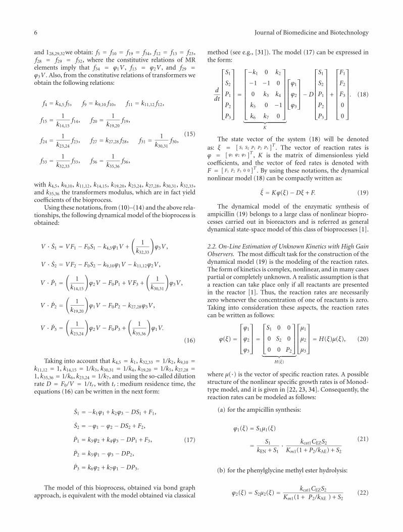
The state vector of the system (18) will be denotedas: ξ = [ S1 S2 P1 P2 P3 ]T . The vector of reaction rates isϕ = [ ϕ1 ϕ2 ϕ3 ]T , K is the matrix of dimensionless yieldcoefficients, and the vector of feed rates is denoted withF = [ F1 F2 F3 0 0 ]T . By using these notations, the dynamicalnonlinear model (18) can be compactly written as:

ξ = Kϕ(ξ)−Dξ + F. (19)

The dynamical model of the enzymatic synthesis ofampicillin (19) belongs to a large class of nonlinear biopro-cesses carried out in bioreactors and is referred as generaldynamical state-space model of this class of bioprocesses [1].

2.2. On-Line Estimation of Unknown Kinetics with High GainObservers. The most difficult task for the construction of thedynamical model (19) is the modeling of the reaction rates.The form of kinetics is complex, nonlinear, and in many casespartial or completely unknown. A realistic assumption is thata reaction can take place only if all reactants are presentedin the reactor [1]. Thus, the reaction rates are necessarilyzero whenever the concentration of one of reactants is zero.Taking into consideration these aspects, the reaction ratescan be written as follows:

ϕ(ξ) =

⎡

⎢⎢⎢⎣

ϕ1

ϕ2

ϕ3

⎤

⎥⎥⎥⎦=

⎡

⎢⎢⎢⎣

S1 0 0

0 S2 0

0 0 P2

⎤

⎥⎥⎥⎦

︸︷︷︸H(ξ)

⎡

⎢⎢⎢⎣

μ1

μ2

μ3

⎤

⎥⎥⎥⎦= H(ξ)μ(ξ), (20)

where μ(·) is the vector of specific reaction rates. A possiblestructure of the nonlinear specific growth rates is of Monod-type model, and it is given in [22, 23, 34]. Consequently, thereaction rates can be modeled as follows:

(a) for the ampicillin synthesis:

ϕ1(ξ) = S1μ1(ξ)

= S1

kEN + S1· kcat1CEZS2

Km1(1 + P2/kAE) + S2

(21)

(b) for the phenylglycine methyl ester hydrolysis:

ϕ2(ξ) = S2μ2(ξ) = kcat1CEZS2

Km1(1 + P2/kAE ) + S2(22)


C:S1

C:S2

C:P3

C:P1

MR1

MR3

MR2

1

1

1

C:P2

Sf

Sf

Sf

Sf

Sf

Sf

Sf

Sf

TF

TF

TF

TF

TF

TF

TF

TF

TF

TF

0

0

0

0

0

25

18

1

2

3

4

5

6

7

8 9

10

11

12

16

1514

13

17

19

20

21

22

23

24

26

2728

29

30

31

32

33

34

35

36

Figure 3: Bond graph model of the enzymatic synthesis of ampicillin. The directions of half arrows correspond to the run of thereaction, from the reactants towards the reaction products. The mass balances are represented by five 0-junctions, and the mass flows ofentering/exiting components are modeled using modulated source flows Sf. The reaction rates are modeled by three modulated two port Relements, MR1, MR2, and MR3. In order to simplify the model representation, the feed flow and the volume are not shown. The bond graphmodel was depicted in 20 sim environment.

(c) for the ampicillin hydrolysis:

ϕ3(ξ) = P2μ3(ξ) = kcat2CEZP2

Km2(1 + S2/kEA ) + P2, (23)

where CEZ represents the enzyme activity (UI/mlgel), kEN,kAE, and kEA are inhibition constants (mM), kcat1, andkcat2 are kinetic constants (mM/UI min), Km1, and Km2 areMichaelis-Menten constants (mM).

However, in practice the reaction rates and/or the specificreaction rates given by the relations (21)–(23) are impreciselyknown. For on-line estimation of these kinetic rates, highgain observers can be designed. Next, the nonlinear model(19) is expressed as:

ξ = KH(ξ)ρ(t)−Dξ + F, (24)

where ρ(t) represents the unknown kinetics of the process. Ifwe suppose that the reaction rates are totally unknown, thenρ(t) = ϕ(t) and H(ξ) = 1. If the structure of the reactionrates is known ϕ(ξ) = H(ξ)μ(ξ), but the specific reactionrates are unknown, then ρ(t) = μ(t) and H(ξ) is the matrixgiven in (20).

The high gain observers design necessitates a factoriza-tion of the model (24) [13, 14, 20]. We will consider that theyield matrix K is of full rank, which is true for our particularmodel, and for general class of bioprocesses’ models is ageneric property. We shall suppose that all state variables are

measured (contrarily, a state estimator can be used). Sincethe yield matrix K is of full rank, then the partition (Ka,Kb)can be considered, such that the submatrix Ka has full rank.Therefore, a partition (ξa, ξb) of the state vector is obtained,and consequently a partition for F is achieved: (Fa,Fb). Then,the system (24) can be written as follows:

ξa = Ka ·H(ξa, ξb) · ρ(t)−D · ξa + Fa,

ξb = Kb ·H(ξa, ξb) · ρ(t)−D · ξb + Fb,(25)

By using this factorization, a highgain observer can beimplemented. The design of highgain observers is done in[13, 14], with supplementary assumptions regarding globalLipschitz conditions, the boundedness of H(ξ) diagonalelements’ away from zero, and so forth. The equations of thenonlinear high gain observer for (24) are obtained as [14]:

˙ξa = KaH(ξa, ξb)ρ−Dξa + Fa − 2θ

(ξa − ξa

),

˙ρ = −θ2 ·[Ka ·H(ξa, ξb)

]−1 ·(ξa − ξa

).

(26)

The high gain observer (26) provides on-line estimates ρfor the unknown kinetics. This on-line estimation algorithmis in fact a copy of the process model, with a corrective term.The observer is simple and the tuning of the gain can bedone by modifying only one design parameter: θ. It should

be noticed that ξa is an “estimate” of ξa, provided by the


algorithm in order to be compared with the real state (ξa ismeasured or provided by a state observer), and the resultingerror to be used in (26).

In order to obtain the equations of the observers forour bioprocess, the next factorization of yield matrix andcorresponding partition are considered [20]:

Ka =

⎡

⎢⎢⎢⎣

−k1 0 k2

−1 −1 0

0 k3 k4

⎤

⎥⎥⎥⎦

, Kb =⎡

⎣k5 0 −1

k6 k7 0

⎤

⎦,

ξa =

⎡

⎢⎢⎢⎣

S1

S2

P1

⎤

⎥⎥⎥⎦

, ξb =⎡

⎣P2

P3

⎤

⎦,

Fa =

⎡

⎢⎢⎢⎣

F1

F2

F3

⎤

⎥⎥⎥⎦

, Fb =⎡

⎣0

0

⎤

⎦.

(27)

Then, for the enzymatic synthesis of ampicillin, twohigh-gain estimators can be derived from (26) [20].

(a) an estimator for the specific reaction rates. In thiscase ρ(t) = μ(t), and H(ξ) is the matrix given in (20). Theequations of the high-gain observer are:

⎡

⎢⎢⎢⎢⎣

˙S1

˙S1

˙P1

⎤

⎥⎥⎥⎥⎦= Ka

⎡

⎢⎢⎢⎣

S1 0 0

0 S2 0

0 0 P2

⎤

⎥⎥⎥⎦

⎡

⎢⎢⎢⎣

μ1

μ2

μ3

⎤

⎥⎥⎥⎦−D

⎡

⎢⎢⎢⎣

S1

S2

P1

⎤

⎥⎥⎥⎦

+

⎡

⎢⎢⎢⎣

F1

F2

F3

⎤

⎥⎥⎥⎦− 2θ

⎡

⎢⎢⎢⎣

S1 − S1

S2 − S2

P1 − P1

⎤

⎥⎥⎥⎦

⎡

⎢⎢⎢⎣

˙μ1

˙μ2

˙μ3

⎤

⎥⎥⎥⎦= −θ2 ·

⎡

⎢⎢⎢⎣Ka ·

⎡

⎢⎢⎢⎣

S1 0 0

0 S2 0

0 0 P2

⎤

⎥⎥⎥⎦

⎤

⎥⎥⎥⎦

−1

·

⎡

⎢⎢⎢⎣

S1 − S1

S2 − S2

P1 − P1

⎤

⎥⎥⎥⎦

,

(28)

(b) a second estimator can be obtained if the entirereaction rate vector is considered unknown. In this caseρ(t) = ϕ(t) and H(ξ) = 1. Then, the equations of thehighgain observer are as follows:

⎡

⎢⎢⎢⎢⎣

˙S1

˙S1

˙P1

⎤

⎥⎥⎥⎥⎦= Ka

⎡

⎢⎢⎢⎣

ϕ1

ϕ2

ϕ3

⎤

⎥⎥⎥⎦−D

⎡

⎢⎢⎢⎣

S1

S2

P1

⎤

⎥⎥⎥⎦

+

⎡

⎢⎢⎢⎣

F1

F2

F3

⎤

⎥⎥⎥⎦− 2θ

⎡

⎢⎢⎢⎣

S1 − S1

S2 − S2

P1 − P1

⎤

⎥⎥⎥⎦

,

⎡

⎢⎢⎢⎣

˙ϕ1

˙ϕ2

˙ϕ3

⎤

⎥⎥⎥⎦= −θ2 · [Ka]−1 ·

⎡

⎢⎢⎢⎣

S1 − S1

S2 − S2

P1 − P1

⎤

⎥⎥⎥⎦.

(29)

The high gain observer (28) needs the on-line measure-ments of S1, S2, P1, and P2. Usually, only the first threeconcentrations are available. Therefore, a state observer isrequired in order to reconstitute the measurements of P2. Forexample, an asymptotic state observer is designed in [31]. Insuch a case, the estimates of P2 provided by the asymptoticobserver will be used in (28). In the case of the high gainobserver (29), only the measurements of S1, S2, and P1 areneeded.

2.3. Adaptive Control Law Design. Concerning the fed-batchbioprocess control, a typical problem is that of generatingthe substrate feed rate profile to optimize a performancecriterion [1]. For our process, the main objective is to obtaina high level of the ampicillin concentration. This goal can beachieved through an optimal control, that is, the calculationof a feeding rate optimal profile. This is unsatisfactory whenthe kinetics is imprecisely known. A possible suboptimalalternative is the adaptive control [1]. In this section, firstly,an exact linearizing control law is obtained. Then, adaptiveversions are implemented, considering that the kinetics areunknown, and by using the kinetics estimators describedbefore.

The exact linearizing control law for the model (18) (orthe model written in the compact form (19)) is obtained ina classical three steps strategy (see [32] for the general pointof view and [1] for bioprocesses). The control goal is that theampicillin concentration y(t) = ξ4(t) = P2(t) to track thedesired substrate trajectory y∗(t) = P∗2 (t), with the dilutionrate as control action: u(t) = D(t). The first step consists inthe achievement of an input-output model of the bioprocess,which is obtained directly from (18):

y = P2 = ξ4 = k5ϕ1(ξ)− ϕ3(ξ)− u · y. (30)

Second, we consider a stable and linear reference modelfor the tracking error y∗ − y:

(y∗ − y

)+ λ(y∗ − y

) = 0, λ > 0. (31)

Finally, the exact linearizing control law is obtained bycalculus of usuch that (30) has the same behavior as (31):

u(t) =(

1y

)

· (k5ϕ1(ξ)− ϕ3(ξ)− λ(y∗ − y

))

=(

1y

)

· (k5μ1(ξ)ξ1 − μ3(ξ)y − λ(y∗ − y

))

=(

1y

)

·(

k5ξ1

kEN + ξ1· kcat1CEZξ2

Km1(1 + y/kAE

)+ ξ2

− kcat2CEZy

Km2(1 + ξ2/kEA ) + y− λ

(y∗ − y

))

,

(32)

where we consider y∗ = const.The exact linearizing control (32) can ensure the achieve-

ment of control goal only if the involved concentrations areon-line measurable and if the reaction rates (or the specificgrowth rates, resp.) are known. Contrarily, the estimations


(mM

)

P1

S1

S2

P3

0 20 40 60 80 100 120 140 160

Time (min)

10

20

30

40

50

60

(a)

(min−1

)(m

in−1

)

µ2

µ3

µ1

0 20 40 60 80 100 120 140 160

Time (min)

0 20 40 60 80 100 120 140 160

Time (min)

1.5

2

2.5

3

0.1

0.2

0.3

0.4

(b)

0

0.5

1

1.5

2

P2

P∗2

(mM

)

0 20 40 60 80 100 120 140 160

Time (min)

(c)

0

0.2

0.4

0.6

0.8

1

1.2

u = D

(min−1

)

0 20 40 60 80 100 120 140 160

Time (min)

(d)

Figure 4: Simulation results—exact linearizing control law. The closed loop system was tested for a step profile of the ampicillinconcentration reference. Panel (a) shows the time evolution of ξ1 = S1, ξ2 = S2, ξ3 = P1, and ξ5 = P3 (i.e., 6-APA, PGME, PG, andmethanol concentrations, resp.). In panel (b), the profiles of specific reaction rates μ1,μ2, and μ3 are depicted. Panel (c) presents the outputy = P2 (ampicillin concentration) versus the reference profile y∗ = P∗2 . Panel (d) shows the control action, that is, the evolution of thedilution rate.

provided by the estimators are needed, and if they areused in the exact linearizing control law, some adaptiveversions of the nonlinear law are obtained. For example, ifthe estimations ρ(t) = μ(t) provided by (28) are used in thecontrol law (32), an adaptive version of this law is obtainedas follows:

u(t) =(

1y

)

· (k5μ1(t)ξ1 − μ3(t)y − λ(y∗ − y

)). (33)

The entire adaptive control algorithm consists of (28)and (33). Regarding the stability and convergence propertiesof the controlled system, these are widely discussed for ageneral class of bioprocesses in [1]. Another version of theadaptive control law (33) is obtained if the full vector ofreaction rates is considered as unknown. In this case, the highgain estimator (29) is used, and the adaptive control law takesthe following form:

u(t) =(

1y

)

· (k5ϕ1(t)− ϕ3(t)− λ(y∗ − y

)). (34)

Therefore, the complete adaptive control algorithmconsists now of (29) and (34). Moreover, when the ampi-cillin concentration cannot be on-line measured, then anasymptotic observer [31] can be used in order to providethe estimates yest, and consequently a version of the adaptivecontroller (33) is obtained as follows:

u(t) =(

1yest

)

· (k5μ1(t)ξ1 − μ3(t)yest − λ(y∗ − yest

)).

(35)

The adaptive control algorithm consists of (28), (35),plus the asymptotic observer.

The design of asymptotic observers is based on massand energy balances without the knowledge of the processkinetics being necessary [1]. More precisely, the design isbased on some useful changes of coordinates, which lead to asubmodel of the process which is independent of the kinetics.Next, the fundaments of the design of an asymptotic observerfor the process (24) will be presented. The maximum stateinformation which can be reconstituted is obtained by usingthe states ξ1 = [S1 P1]T considered as measurable. Therefore,

the vector of unavailable states is ξ2 =[S2 P2 P3 ]T ; these


0

0.5

1

1.5

2

2.5(m

M)

P2

P∗2

0 20 40 60 80 100 120 140 160

Time (min)

(a)

0.08

0.1

0.12

0.14

0.16

0.18

0.2

(min−1

)

µ1

µ1

0 20 40 60 80 100 120 140 160

Time (min)

(b)

0.2

0.3

0.4

0.5

0.6

0.7

0.8

(min−1

)

µ2

µ2

0 20 40 60 80 100 120 140 160

Time (min)

(c)

2

2.5

3

3.5

4

4.5

5

(min−1

)

µ3

µ3

0 20 40 60 80 100 120 140 160

Time (min)

(d)

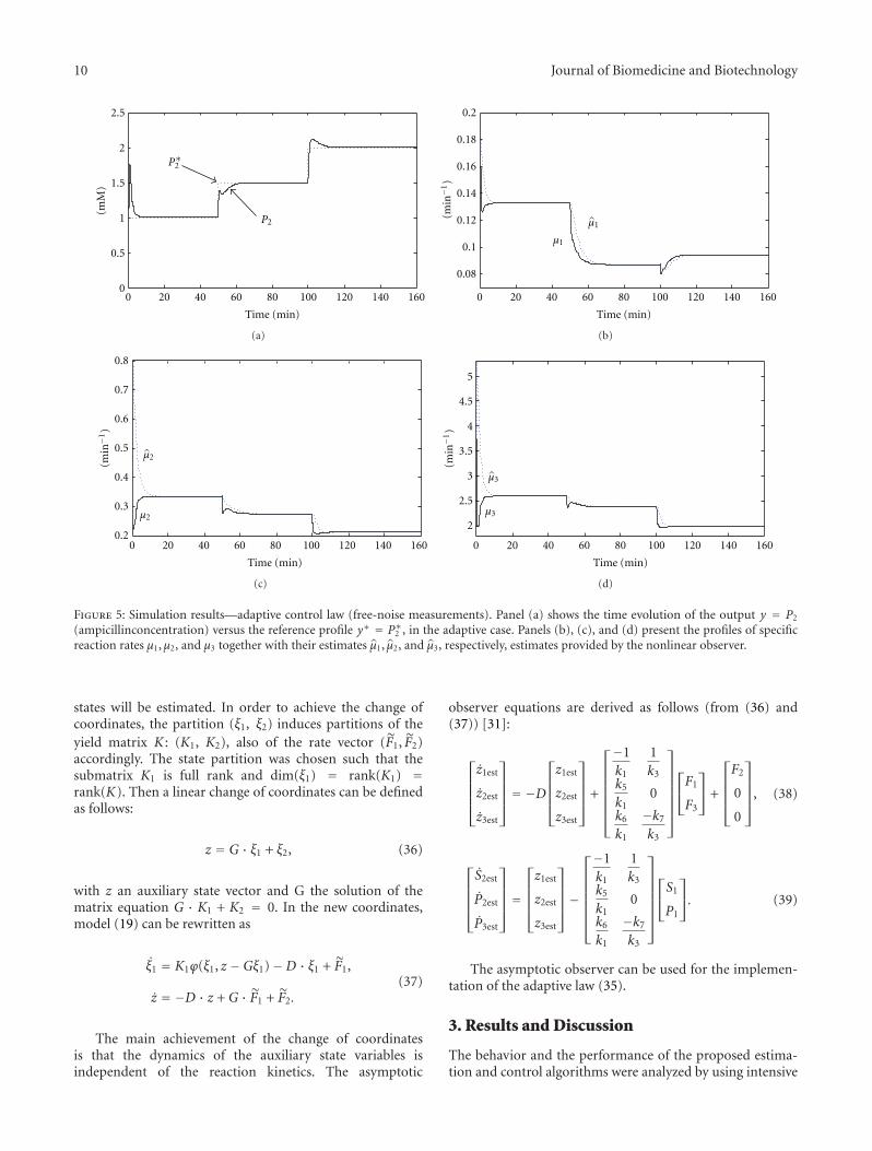
Figure 5: Simulation results—adaptive control law (free-noise measurements). Panel (a) shows the time evolution of the output y = P2

(ampicillinconcentration) versus the reference profile y∗ = P∗2 , in the adaptive case. Panels (b), (c), and (d) present the profiles of specificreaction rates μ1,μ2, and μ3 together with their estimates μ1, μ2, and μ3, respectively, estimates provided by the nonlinear observer.

states will be estimated. In order to achieve the change ofcoordinates, the partition (ξ1, ξ2) induces partitions of theyield matrix K : (K1, K2), also of the rate vector (F1, F2)accordingly. The state partition was chosen such that thesubmatrix K1 is full rank and dim(ξ1) = rank(K1) =rank(K). Then a linear change of coordinates can be definedas follows:

z = G · ξ1 + ξ2, (36)

with z an auxiliary state vector and G the solution of thematrix equation G · K1 + K2 = 0. In the new coordinates,model (19) can be rewritten as

ξ1 = K1ϕ(ξ1, z −Gξ1)−D · ξ1 + F1,

z = −D · z + G · F1 + F2.(37)

The main achievement of the change of coordinatesis that the dynamics of the auxiliary state variables isindependent of the reaction kinetics. The asymptotic

observer equations are derived as follows (from (36) and(37)) [31]:

⎡

⎢⎢⎢⎣

z1est

z2est

z3est

⎤

⎥⎥⎥⎦= −D

⎡

⎢⎢⎢⎣

z1est

z2est

z3est

⎤

⎥⎥⎥⎦

+

⎡

⎢⎢⎢⎢⎢⎢⎣

−1k1

1k3

k5

k10

k6

k1

−k7

k3

⎤

⎥⎥⎥⎥⎥⎥⎦

⎡

⎣F1

F3

⎤

⎦ +

⎡

⎢⎢⎢⎣

F2

0

0

⎤

⎥⎥⎥⎦

, (38)

⎡

⎢⎢⎢⎣

S2est

P2est

P3est

⎤

⎥⎥⎥⎦=

⎡

⎢⎢⎢⎣

z1est

z2est

z3est

⎤

⎥⎥⎥⎦−

⎡

⎢⎢⎢⎢⎢⎢⎣

−1k1

1k3

k5

k10

k6

k1

−k7

k3

⎤

⎥⎥⎥⎥⎥⎥⎦

⎡

⎣S1

P1

⎤

⎦. (39)

The asymptotic observer can be used for the implemen-tation of the adaptive law (35).

3. Results and Discussion

The behavior and the performance of the proposed estima-tion and control algorithms were analyzed by using intensive


0 20 40 60 80 100 120 140 1600

0.5

1

1.5

2

2.5

Time (min)

P2

P∗2

(mM

)

(a)

0 20 40 60 80 100 120 140 160

Time (min)

0.06

0.08

0.1

0.12

0.14

0.16

0.18

0.2

0.22

(min−1

)

µ1

µ1

(b)

0 20 40 60 80 100 120 140 160

Time (min)

0.2

0.3

0.4

0.5

0.6

0.7

0.8

(min−1

)

µ2

µ2

(c)

0 20 40 60 80 100 120 140 160

Time (min)

1.5

2

2.5

3

3.5

4

4.5

5

5.5

(min−1

)

µ3

µ3

(d)

Figure 6: Simulation results—adaptive control law (noisy measurements). Panel (a) shows the profile of the output y = P2 (ampicillinconcentration) versus the reference y∗ = P∗2 , in the adaptive case, when noisy measurements of S1 and S2 are used in both estimation andcontrol algorithms. Panels (b), (c), and (d) present the profiles of specific reaction rates μ1,μ2, and μ3 together with their estimates μ1, μ2 andμ3, respectively, in the case of noisy measurements.

Table 1: Bioprocess parameters values.

Parameter Value

kcat1 0.546 (mM/UI min)

kcat2 1.857 (mM/UI min)

CEZ 30 (UI/mlgel)

kEN 22.57 (mM)

kAE 1.05 (mM)

kEA 32.13 (mM)

Km1 15.32 (mM)

Km2 12.83 (mM)

F1 2 (mM/min)

F2 2.5 (mM/min)

F3 1 (mM/min)

k1 0.7

ki, i = 2, . . ., 7 1

simulations. The simulations were performed in MATLABenvironment (registered trademark of The MathWorks Inc.,USA). The fed-batch bioprocess has been simulated bynumerical integration of the basic model equations (18),

(21)–(23). The values of kinetic parameters and of yieldcoefficients used in simulations are presented in Table 1[23, 31].

Three simulation scenarios were taken into considera-tion.

(i) The exact linearizing control law (32) was imple-mented for the bioprocess (18), with the design parameterλ = 3. The closed loop system was tested for a step profileof the ampicillin concentration reference. This simulationcase is a kind of benchmark, because all the parameters andthe reaction rates are considered to be known (and givenby the relations (21)–(23)). A parametric disturbance wasconsidered in the feed rate F2, which has a 20% decrease of itsnominal value (between t = 50 min and t = 100 min). Thesimulation results are presented in Figure 4. Panel (a) showsthe time profiles of ξ1 = S1, ξ2 = S2, ξ3 = P1, and ξ5 =P3 (i.e., 6-APA, PGME, PG, and methanol concentrations,resp.). In panel (b) the evolution of the specific reactionrates is depicted, while in panel (c) the output (ampicillinconcentration) versus the reference profile is shown. Panel(d) presents the control action, that is, the evolution of thedilution rate. From these simulation results, it can be seen avery good behavior of the controlled bioprocess.


Table 2: Performance criterion results (free-noise data).

Tuning parameter I1 I2 I3

θ = 1 0.01029 0.03230 0.08333

θ = 2 0.00321 0.01789 0.03768

θ = 5 0.00225 0.00849 0.01124

θ = 50 0.00039 0.00052 0.00126

Table 3: Performance criterion results (noisy measurements).

Tuning parameter I1 I2 I3

θ = 1 0.06370 0.03392 0.16932

θ = 2 0.09196 0.02198 0.35544

θ = 5 0.62471 0.24404 1.59703

θ = 50 — (divergent) — (divergent) —(divergent)

(ii) In the second simulation scenario, an adaptiveversion of the control law was implemented in the sameconditions as in previous case. This adaptive controllerconsists of the high gain observer (28) and the control law(33). Therefore, the specific growth rates μ1, μ2, and μ3 wereconsidered to be unknown. The kinetic expressions (21)–(23) were introduced only for simulation; so these modelswere not used in the process of observer design. The maingoal of the estimator (28) is to reconstitute the time evolutionof μ1, μ2, and μ3 from the measurements of S1, S2, P1, and P2

obtained from the simulation.The value of the tuning parameter was set to θ = 2.

The on-line estimations provided by the high gain observer(28) were used in the control law (33)—in fact only μ1 andμ3 are used here. The results in this simulation case areshown in Figure 5. Panel (a) presents the output versus thereference profile, and panels (b), (c), and (d) show the timeevolution of the estimated specific reaction rates versus their“true” profiles. In this scenario, the obtained results are good,despite the uncertainty in the bioprocess kinetics.

(iii) In order to test the robustness of the proposedestimation and control algorithms to noisy measurements,the behavior of the controlled bioprocess was also analyzedfor noisy data of S1 and S2. The measurements of theseconcentrations are considered to be vitiated by an additiveGaussian noise, with zero mean and amplitude equal to 5%of the free-noise values. The same version of the adaptivecontrol law (28), (33) was used in this case. The obtainedresults are presented in Figure 6. As in previous case, panel(a) shows the output versus the reference profile, and panels(b), (c), and (d) depict the time evolution of the estimatedspecific reaction rates versus their “true” profiles.

It can be seen that the behavior of the controlledprocess is quite good, in spite of the combined action ofnoisy measurements, parametric disturbance, and kineticsuncertainty. The specific reaction rates μ1 and μ3 seem to bea little bit more sensible to noise.

A lot of supplementary simulations were performed forthe other versions of adaptive control laws, such as (29), (34)and (28), (35). In all situations, a good behavior of the closed

loop system was obtained. The results illustrate that the high-gain observer provides accurate estimates of the kinetic rates.It can be seen that the noisy measurement induces somenoisy estimates of the kinetics, but the noise effect is limited(however, this effect can be reduced for lower values ofthe tuning parameter). Several comparisons and commentsregarding the behavior and the performance of the on-lineestimation strategy can be achieved. Some remarks can bedone by visualization of estimation errors μ1 = μ1 − μ1, μ2 =μ2− μ2 and μ3 = μ3− μ3. However, accurate comparisons canbe realized by considering a criterion, for example, one basedon averaged square estimation errors [3]:

I1 = 1TS

∫ TS

0μ2

1(t)dt,

I2 = 1TS

∫ TS

0μ2

2(t)dt,

I3 = 1TS

∫ TS

0μ2

3(t)dt,

(40)

where TS is the total simulation time.The values of I1, I2, and I3 computed for different values

of tuning parameter and free noise data are given in Table 2,and for vitiated measurements in Table 3. It results that theprecision can be increased if the tuning parameter is bigger.The problem for a large value of θ is that the observerbecomes noise sensitive. Notice that the estimation error canbe made as small as wished if we choose greater values ofθ. The problem for a large value of θ is that the observerbecomes noise sensitive. Therefore, the value of the tuningparameter is a compromise between a good estimation andthe noise rejection. The obtained results concerning the noisesensitivity of the high gain observers are similar with thosediscussed in several works, such as [35–38].

4. Conclusions

The bond graph modeling approach constitutes a notewor-thy option to the classical modeling in the case of complexbioprocesses. The ampicillin synthesis process was modeledin a natural way via pseudo bond graphs, and the obtainedmodel was used for estimators and controllers design. Oneof the key advantages of the bond graph modeling of bio-processes is the possibility to reuse the models, for example,in the interconnected bioreactors. The application of thisfeature is beyond of the scope of the present paper, but it is ofcrucial importance in other bioprocesses. However, it shouldbe mentioned that the obtained model is only validatedfor the specific enzyme preparation used (but the proposedmethod can be utilized with adequate modifications whenthe enzyme is changed).

To overcome problems such as the kinetics uncertain-ties and the lack of on-line measurements, a high gainobserver was designed and implemented for the on-linereconstruction of the specific reaction rates. The advantagesof this kind of estimator are the simplicity of design,the good convergence and stability properties, and theaccuracy of estimates (especially for free noise data). Another


important advantage is the fact that the tuning of one singledesign parameter is necessary. The estimation results can beimproved if the tuning parameter is chosen higher in value,but only if the measurements are free noise. Contrarily, theobserver becomes noise sensitive and it is possible that theestimates of kinetics cannot be utilized in the control lawdesign.

The simulation results show a good behavior of theadaptive controlled ampicillin synthesis bioprocess. Theproposed adaptive control law was obtained by combiningan exact linearizing control law with the kinetics estimator.The control goal, that is, the preservation of a high ampicillinconcentration, is achieved despite the action of disturbancesand noisy measurements. The bond graph modeling esti-mation and control strategies can be also applied to otherprocesses belonging to the nonlinear class of bioprocessesconsidered in the present study.

Acknowledgment

This work was supported by CNCSIS UEFISCDI, Romania,Projects PNII—IDEI 548/2008 and PNII—RU 108/2010.

References

[1] B. Bastin and D. Dochain, On-Line Estimation and AdaptiveControl of Bioreactors, Elsevier, Amsterdam, The Netherlands,1990.

[2] K. Schugerl, “Progress in monitoring, modeling and control ofbioprocesses during the last 20 years,” Journal of Biotechnology,vol. 85, no. 2, pp. 149–173, 2001.

[3] D. Selisteanu, M. Roman, and D. Sendrescu, “Pseudo BondGraph modelling and on-line estimation of unknown kineticsfor a wastewater biodegradation process,” Simulation Mod-elling Practice and Theory, vol. 18, no. 9, pp. 1297–1313, 2010.

[4] D. Karnopp and R. Rosenberg, System Dynamics: A UnifiedApproach, John Wiley, New York, NY, USA, 1974.

[5] W. Borutzky, Bond Graph Methodology. Development andAnalysis of Multidisciplinary Dynamic System Models, Springer,London, UK, 2009.

[6] J. L. Balino, “Galerkin finite element method for incompress-ible thermofluid flows framed within the bond graph theory,”Simulation Modelling Practice and Theory, vol. 17, no. 1, pp.35–49, 2009.

[7] F. Couenne, C. Jallut, B. Maschke, P. C. Breedveld, and M.Tayakout, “Bond graph modelling for chemical reactors,”Mathematical and Computer Modelling of Dynamical Systems,vol. 12, no. 2-3, pp. 159–174, 2006.

[8] C. Heny, D. Simanca, and M. Delgado, “Pseudo-bond graphmodel and simulation of a continuous stirred tank reactor,”Journal of the Franklin Institute, vol. 337, no. 1, pp. 21–42,2000.

[9] V. Dıaz-Zuccarini, D. Rafirou, J. LeFevre, D. R. Hose, and P. V.Lawford, “Systemic modelling and computational physiology:the application of Bond Graph boundary conditions for 3Dcardiovascular models,” Simulation Modelling Practice andTheory, vol. 17, no. 1, pp. 125–136, 2009.

[10] X. Zhang, K. A. Hoo, and D. Overland, “Bond Graph modelingof an integrated biological wastewater treatment system,” inProceedings of the American Institute of Chemical EngineersAnnual Meeting, p. 479e, San Francisco, Calif, USA, 2006.

[11] M. Roman and D. Selisteanu, “Pseudo bond graph mod-elling of wastewater treatment bioprocesses,” SIMULATION—Transactions of the Society of Modeling and Simulation Interna-tional, vol. 88, no. 2, pp. 233–251, 2012.

[12] C. Pichardo-Almarza, A. Rahmani, G. Dauphin-Tanguy, andM. Delgado, “Proportional-integral observer for systemsmodelled by bond graphs,” Simulation Modelling Practice andTheory, vol. 13, no. 3, pp. 179–211, 2005.

[13] M. Farza, K. Busawon, and H. Hammouri, “Simple nonlinearobservers for on-line estimation of kinetic rates in bioreac-tors,” Automatica, vol. 34, no. 3, pp. 301–318, 1998.

[14] J. P. Gauthier, H. Hammouri, and S. Othman, “A simpleobserver for nonlinear systems applications to bioreactors,”IEEE Transactions on Automatic Control, vol. 37, no. 6, pp.875–880, 1992.

[15] N. P. Guerra, P. Fajardo, C. Fucinos et al., “Modelling thebiphasic growth and product formation by enterococcusfaecium CECT 410 in realkalized fed-batch fermentations inwhey,” Journal of Biomedicine and Biotechnology, vol. 2010,Article ID 290286, 16 pages, 2010.

[16] D. Sendrescu, E. Petre, and E. Bobasu, “Structural identifia-bility of some biotechnological systems,” in Proceedings of TheWSEAS International Conference on Environment, Ecosystemsand Development (EED ’07), pp. 49–55, Puerto de la Cruz,Spain, 2007.

[17] H. K. Khalil, “High-gain observers in nonlinear feedbackcontrol,” in Proceedings of the International Conference onControl, Automation and Systems, pp. 47–57, Seoul, Republicof Korea, 2008.

[18] D. Selisteanu, E. Petre, and V. B. Rasvan, “Sliding modeand adaptive sliding-mode control of a class of nonlinearbioprocesses,” International Journal of Adaptive Control andSignal Processing, vol. 21, no. 8-9, pp. 795–822, 2007.

[19] D. Sendrescu, “Nonlinear model predictive control of adepollution bioprocess,” in Proceedings of 3rd Pacific-AsiaConference on Circuits, Communications and System (PACCS’11), vol. 1, pp. 1–4, Wuhan, China, 2011.

[20] D. Selisteanu, E. Petre, M. Roman, D. Popescu, and E. Bobasu,“On-line estimation of unknown kinetics for the enzymaticsynthesis of ampicillin,” in Proceedings of the InternationalCarpathian Control Conference, pp. 335–340, Velke Karlovice,Czech Republic, 2011.

[21] J. P. Hou and J. W. Poole, “The amino acid nature of ampicillinand related penicillins,” Journal of Pharmaceutical Sciences, vol.58, no. 12, pp. 1510–1515, 1969.

[22] A. L. O. Ferreira, L. R. B. Goncalves, R. C. Giordano, andR. L. C. Giordano, “A simplified kinetic model for theside reactions occurring during the enzymatic synthesis ofampicillin,” Brazilian Journal of Chemical Engineering, vol. 17,no. 4, pp. 835–839, 2000.

[23] L. R. B. Goncalves, R. Fernandez-Lafuente, J. M. Guisan, andR. L. C. Giordano, “A kinetic study of synthesis of amoxicillinusing penicillin G acylase immobilized on agarose,” AppliedBiochemistry and Biotechnology, vol. 84-86, pp. 931–945, 2000.

[24] S. A. W. Jager, P. A. Jekel, and D. B. Janssen, “Hybrid penicillinacylases with improved properties for synthesis of β-lactamantibiotics,” Enzyme and Microbial Technology, vol. 40, no. 5,pp. 1335–1344, 2007.

[25] J. M. Guisan, “Immobilization of enzymes as the 21st Centurybegins: an already solved problem or still an exciting chal-lenge?” in Immobilization of Enzymes and Cells, J. M. Guisan,Ed., vol. 22 of Methods in Biotechnology, pp. 1–13, 2006.

[26] K. Buchholz, V. Kasche, and U. T. Theo Bornscheuer,Biocatalysts and Enzyme Technology, Wiley-VCH, Weinheim,Germany, 2005.


[27] M. Terreni, J. G. Tchamkam, U. Sarnataro, S. Rocchietti,R. Fernandez-Lafuente, and J. M. Guisan, “Influence ofsubstrate structure on PGA-catalyzed acylations. Evaluation ofdifferent approaches for the enzymatic synthesis of cefonicid,”Advanced Synthesis and Catalysis, vol. 347, no. 1, pp. 121–128,2005.

[28] C. Mateo, J. M. Palomo, G. Fernandez-Lorente, J. M. Guisan,and R. Fernandez-Lafuente, “Improvement of enzyme activ-ity, stability and selectivity via immobilization techniques,”Enzyme and Microbial Technology, vol. 40, no. 6, pp. 1451–1463, 2007.

[29] K. Hernandez and R. Fernandez-Lafuente, “Control of proteinimmobilization: coupling immobilization and site-directedmutagenesis to improve biocatalyst or biosensor perfor-mance,” Enzyme and Microbial Technology, vol. 48, no. 2, pp.107–122, 2011.

[30] G. Volpato, R. C. Rodrigues, and R. Fernandez-Lafuente, “Useof enzymes in the production of semi-synthetic penicillinsand cephalosporins: drawbacks and perspectives,” CurrentMedicinal Chemistry, vol. 17, no. 32, pp. 3855–3873, 2010.

[31] E. C. Ferreira, Identification and adaptive control of biotechno-logical processes, Ph.D. thesis, University of Porto, 1995.

[32] A. Isidori, Nonlinear Control Systems, Springer, London, UK,3rd edition, 1995.

[33] A. K. P. B. Siqueira, L. R. B. Goncalves, R. C. Giordano, R.L. C. Giordano, and A. L. O. Ferreira, “Ampicillin synthesiscatalyzed by penicillin acylase: effect of pH and type of carrierson selectivity and yield,” in Proceedings of 2nd MercosurCongress on Chemical Engineering, Brazil, 2005.

[34] M. P. De Arruda Ribeiro and R. D. C. Giordano, “Variationalcalculus (optimal control) applied to the optimization ofthe enzymatic synthesis of ampicillin,” Brazilian Archives ofBiology and Technology, vol. 48, pp. 19–28, 2005.

[35] J. H. Ahrens and H. K. Khalil, “High-gain observers in thepresence of measurement noise: a switched-gain approach,”Automatica, vol. 45, no. 4, pp. 936–943, 2009.

[36] V. Andrieu, L. Praly, and A. Astolfi, “High gain observerswith updated gain and homogeneous correction terms,”Automatica, vol. 45, no. 2, pp. 422–428, 2009.

[37] N. Boizot, E. Busvelle, and J. P. Gauthier, “An adaptive high-gain observer for nonlinear systems,” Automatica, vol. 46, no.9, pp. 1483–1488, 2010.

[38] M. Farza, M. Oueder, R. Benabdennour, and M. M’Saad,“High gain observer with updated gain for a class of MIMOsystems,” International Journal of Control, vol. 84, no. 2, pp.270–280, 2011.

Submit your manuscripts athttp://www.hindawi.com

Hindawi Publishing Corporationhttp://www.hindawi.com Volume 2014

Anatomy Research International

PeptidesInternational Journal of


Hindawi Publishing Corporation http://www.hindawi.com

International Journal of

Volume 2014

Zoology


Molecular Biology International

GenomicsInternational Journal of


The Scientific World JournalHindawi Publishing Corporation http://www.hindawi.com Volume 2014


BioinformaticsAdvances in

Marine BiologyJournal of



Signal TransductionJournal of


BioMed Research International

Evolutionary BiologyInternational Journal of



Biochemistry Research International

ArchaeaHindawi Publishing Corporationhttp://www.hindawi.com Volume 2014


Genetics Research International


Advances in

Virolog y

Hindawi Publishing Corporationhttp://www.hindawi.com

Nucleic AcidsJournal of

Volume 2014

Stem CellsInternational



Enzyme Research


International Journal of

Microbiology

enzymaticsynthesisofampicillin:nonlinearmodeling...

Documents