envr 322 oceanography laboratory
TRANSCRIPT

ECSI 322 – Oceanography Laboratory - Manual 1
ESCI 322 - Oceanography Laboratory
Laboratory Manual
Prepared by David Shull
Department of Environmental Sciences
Huxley College of the Environment
Western Washington University
Bellingham, WA 98225
Last update: September 17, 2014

ECSI 322 – Oceanography Laboratory - Manual 2
ESCI 322 - Introduction to Oceanography Laboratory
Course Syllabus Instructor: David Shull
Office: ES 445, ext. 3690
Email: [email protected]
OBJECTIVES:
1. Acquire first-hand experience with oceanographic research methods
2. Become familiar with marine organisms and coastal processes in Puget Sound
3. Learn field and laboratory techniques
4. Practice scientific writing (writing proficiency course - WP3)
5. Use oceanographic methods to address local marine environmental problems.
COURSE OVERVIEW:
We will use oceanographic methods to study ecosystem functions and environmental problems
in the marine waters near Bellingham. Students will write reports addressing these issues. Many
of our "labs" will take place in the field, either on a boat or at the Shannon Point Marine Center.
EVALUATION GUIDELINES:
Assignments:
Students will be evaluated based on the completion of several lab reports, a smaller lab
assignment, and “pre-laboratory” assignments. Each assignment will be typed, although figures
and graphs may be drawn by hand. The reports will follow the standard scientific format;
abstract, introduction, methods, results, discussion, references. For some of the reports, a draft
of a portion of the results will be handed in first for evaluation and comments as a component of
pre-laboratory reports. Comments on the draft of the results section are intended to aid students
in the completion of the final reports. Reports must be turned in on time to receive full credit.
Late reports will receive a 10% grade reduction each day until the report is turned in. Details on
the format of the major reports are given in the section of the syllabus entitled "Laboratory
Report Format". Read this section carefully before you begin. The first assignment will be
completed in question-and-answer format. All reports should be typed, double-spaced, and
checked for correct grammar and spelling. You should read through the assignment, make notes,
and think through the organization of all your responses before writing. Pre-laboratory
assignments needn’t be typed but must be handed in at the beginning of each laboratory period to
receive credit.
Contributions of assignments to final grade:
Full lab reports 80%
Pre-lab assignments 20%
Approximate grading scale:
93-100 A 90-92 A- 88-89 B+ 83-87 B 80-82 B- 78-79 C+
73-77 C 69-72C- 67-68 D+ 61-66 D 57-60 D- 0-56 F

ECSI 322 – Oceanography Laboratory - Manual 3
Policy for late assignments and reports:
Final reports will lose 10% of the final grade for each late day until turned in. (Reports received
after 5 PM will be picked up the next day.) Pre-labs will not be accepted late.
LAB REPORT FORMAT
A laboratory report is a document in the form of a scientific paper. Writing and publishing
research results is just as important as conducting research in the first place, for if results are not
made available to others, they are of little value. For ease of communication, there is a generally
accepted format for writing science that we will follow in this course. Mastery of scientific
writing skills is a vital component of becoming a scientist. Scientific papers have 7 sections:
Title, Abstract, Introduction, Materials and Methods, Results, Discussion, and References. These
headings should be placed at the beginning of each section in your report (except “Title”).
Brief descriptions of the seven sections follow.
Title
The title should be a self-contained explanation of the information presented in your paper. It
must contain enough detail to be informative, without being so long as to be incomprehensible.
Avoid vagueness at all cost.
Too short: Vertical profiling
Too vague: Oceanography laboratory report #1
Too long: A student investigation of the effects of the Nooksack River on the vertical and
horizontal distribution of temperature, salinity, density, nutrients, and dissolved oxygen in
Bellingham, Bay, WA, in November, 2014.
Abstract
The abstract is a short one- to two-paragraph essay that summarizes the major findings of the
paper. The abstract is important because it may be the only part of the paper someone will read.
If the abstract is interesting, concise, well-written, and accurately summarizes the content of your
work, it could motivate someone with an interest in the topic to read the rest of the paper. The
abstract must not include ideas or information that is not included in the rest of the paper. It
should briefly discuss the motivation for the study, methods, major results, and inferences drawn
from those findings. If the development of new methods is an important part of the paper, they
should be described in the abstract as well. References are not typically cited in the abstract.
One way to organize an abstract is to simply write a sentence or two summarizing your
introduction (why you did it), methods (what you did), results (what you observed), and
discussion (what it means).
Introduction
The introduction sets the stage for the presentation of your research results and their
interpretation. It must include some background information, to bring the reader up to speed on
the general issues, some specifics, to acquaint the reader with your particular investigation, and
the questions or hypotheses that you will be addressing with the data. Effective introductions are
usually short (several paragraphs). You must cite published papers from the peer-reviewed
literature in your introduction. Internet sites are rarely cited in the introduction.
ECSI 322 – Oceanography Laboratory - Manual 4
Background information: What is the general problem that is being studied? What is your
specific approach to that problem? If there is relevant background literature (other important
scientific papers that set the stage for your work), this is the place to briefly summarize their
findings and importance. However, the introduction should not be an exhaustive literature
review. Keep the introduction focused on the problem you are addressing.
Specifics: This section will vary depending on the type of research you are presenting. In an
environmental study, you should let the reader know where and when you were working, and
what the environment was like in a general way. If you were presenting the results of an
experiment with organisms, you should describe the species used and the general approach. Try
to develop a logical flow from the “big picture” of background information to the specifics of the
system you studied.
Research questions: End your introduction with a concise summary of the research questions,
hypotheses or goals. You will come back to these in the concluding paragraph of your
discussion.
Materials and Methods
The materials and methods section describes how, when, where and what you did. Describe the
procedures, equipment, and experimental set-ups in enough detail that the work could be
repeated by another scientist, but without extraneous detail. List the methods or procedures
chronologically (i.e. in the order in which you did them). Be sure to include information about
numbers of replicate treatments or observations, types of instruments and equipment used, etc. If
statistical analyses were performed, state the statistical methods used and the data to which they
were applied. Use the past tense.
The methods section is NOT a sequential recounting of everything you did. It does not tell
a story or go into the nitty-gritty details unless these are important for the reader to know
in order to repeat the work. Instead, it works better if you organize your methods sections
around specific tasks. For example, "Concentrations of nutrients (ammonium, nitrate+nitrite,
and phosphate) were measured following the methods of Parsons et al. (1984). Samples were
collected from Niskin bottles into clean and sample-water rinsed 100-ml polyethylene bottles.
Sample water was first filtered through a gf/c glass-fiber filter (nominal diameter 0.7-μm) and
was frozen prior to analysis. Ammonium was measured on thawed samples as follows..." The
idea is to briefly tell the reader the important details of your methodology. The following
structure is NOT acceptable: “First we collected water samples from a Niskin bottle. We then
filtered the samples through a gf/c glass fiber filter. Samples were frozen for one week and then
the following week we measured nutrient concentrations in the analytical lab at the Shannon
Point Marine Center.” The problem with the second example is that it includes information that
is not critical such as the location where samples were analyzed. (It is not necessary for all
marine scientists to measure their nutrient samples at SPMC.) It also describes the activities
chronologically as though the order in which the activities were performed was critical.
Methods that are already published can be referred to with a reference; only deviations from the
published method need to be described in your paper. (“Nitrate was measured by the method of
Parsons et al. (1984), except that reagent additions were scaled to a sample volume of 5 ml.”)

ECSI 322 – Oceanography Laboratory - Manual 5
You can reference lab handouts, but be sure they are cited in the reference section. You do not
need to explain things that are not necessary for understanding or repeating the work (“The
group was divided in half and group A went out in the boat first, then group B.”) You can use
either passive voice (“Salinities were measured at 1-m intervals.”) or active voice (“We
measured salinities at 1-m intervals.”), but I prefer active voice as it is generally more precise.
Results
The results section is the heart of the paper. This is where you tell the reader everything that you
found: what, when, where. Interpretation of those data, however, is left for the discussion
section. This allows the reader to formulate her or his own interpretation before reading yours.
The results section consists of tables and graphs that summarize your data (not raw data), and
text that describes and highlights the major features of those data. The results section text is often
fairly short. Use the past tense here, as the observations were made in the past (e.g: Surface water
salinity was lower at stations in northern Bellingham Bay near the mouth of the Nooksack River
compared to stations further south.) Results sections are much more fun to read if you use this
section to tell the reader a story about what you found. Although most of the text will describe
the results summarized in figures and tables, try to be interesting as you lead the reader through
your discoveries.
Figures and Tables: Each figure (map, diagram, or graph) and table in a results section should
have a “reason for being.” Don’t present data just because you collected it; present data only if it
you refer to it in the text and it contributes to the story that you are telling in your paper. In
general, figures are plotted with the independent variable on the x axis. Vertical profiles in
oceanography have a special format in which the independent variable (depth is plotted on the y-
in axis. (We'll discuss this more in class.) Each table and figure should be readily
understandable without reference to the text. Each should have a consecutive number (Fig. 1, 2,
3…); tables are numbered separately from figures. Finally, each figure and table should have a
caption (sometimes called a ‘legend’) that concisely describes the content (e.g.: Fig. 2. Average
rates of respiration (±1 standard deviation) over time for the anemone Anthopleura elegantissima
at 10ºC.)
Text: The text of the results section should weave the data presented in figures and tables into a
coherent story. Prepare the figures and tables first, and then write the text. Do not reiterate all the
details of the data; rather, tell the story that describes the major features and any clear trends or
patterns. Refer directly to the appropriate figures and tables, by number, in your text. The first
figure referred to should be Fig. 1, the second Fig. 2, etc. Keep the writing simple and direct.
Don't use the word Figure or Table as the subject of a sentence, e.g., Figure 1 shows the
locations of the sampling sites, because this ruins the narrative style. Instead, tell the story and
refer to figures in parentheses.
Examples:
Not good: The graph of temperature versus depth looks linear near the bottom.
Still not so good: Fig. 1 shows that temperature was constant with depth near the bottom.
Better: Temperature was constant throughout the bottom 5 m of the water column (Fig. 1).
Incorrect: A paired t-test showed that the respiration measurements were significantly different
at the 95% confidence level.
Good: Growth rates in the anemones were higher at 12ºC than at 10ºC (t-test, t[8]=2.9, p = 0.02).
ECSI 322 – Oceanography Laboratory - Manual 6
Discussion
In the discussion you interpret your results: tell the reader what they mean and why they are
important. In this section you should answer “why?” and “how?” questions about your data. For
example, why was the temperature different at the top relative to the bottom of the water
column? Why did the respiration rate of the anemones increase with temperature? Here readers
should discover the answers to your original questions or hypotheses as set forth in the
introduction. The discussion section is also where you compare your findings to those of others,
as reported in the scientific literature. This means you must cite published papers in your
discussion. You may also want or need to discuss short-comings in your methods, or the need
for further testing. This latter should not, however, be the main focus of the section. The
discussion section should be a general synthesis of your findings and their importance. Do not
restate your results. The key word is interpretation. This section is usually the hardest to write;
think it through carefully and prepare an outline before you begin. One effective technique is to
start the section with your strongest or most important finding.
References
This section is an alphabetical listing, by first author’s last name, of the references cited in your
paper. There are two ways to cite a paper in your text. Example 1: Several other species of
anemone are known to have respiration rates that increase with temperature (Matthews, 2003;
Smith and Wesson, 2014). Example 2: Our findings of lower respiration rate at lower
temperatures agreed with those of Matthews (2003). If there are more than two authors, use the
term et al. (an abbreviation of et alias, “and others”) after the name of the first author: Michaels
et al. (1994) or (Michaels et al., 1994). Journals have their own specified format for listing
references, which should be followed when submitting a paper to that journal. For our purposes,
you can use the format below.
Journal article:
Name(s) of author(s). Date. Title of article. Title of journal (may be abbreviated). Vol #: pages.
Example: Lenington, S. 1979. Effect of holy water on the growth of radish plants. Psychological Reports 45: 381-
382.
Book:
Name(s) of authors. Date. Title of book. Publisher, Location (city) of publisher, # of pages in
entire book.
Example: Povinelli, D. J. 2000. Folk Physics for Apes: The Chimpanzee's Theory of How the World Works. Oxford
University Press, New York, 391 pp.
Chapter from a book in which each chapter has a different author and the book has an editor:
Name(s) of authors. Date. Title of chapter. In: editor(s), Book Title. Publisher, Location (city) of
publisher, pages.
Example: Jumars, P. A. 1993. Gourmands of mud: Diet selection in marine deposit feeders. In: R.N. Hughes (Ed.),
Mechanisms of Diet Choice. Blackwell Scientific Publishers, Oxford. pp. 124-156.

ECSI 322 – Oceanography Laboratory - Manual 7
ESCI 322 Lab Assignment : Waves and Coastal Processes
Objectives: During this laboratory session we will study some of the properties of waves. We
will create our own experiments in wave tanks, altering variables known to affect wave
properties (see below), to explore the mathematical relationships among those properties. We
will also set up an experiment to simulate the effects of waves on coastlines.
Broader learning objectives: Compare measurements with theory and evaluate their agreement.
Develop hypotheses as a group and then conduct a laboratory experiment to test them. Begin to
develop skill using Microsoft Excel as a tool for analyzing and displaying data.
Terminology: -Wave height (H) is the vertical change in height between the wave crest and the wave trough.
-Wave amplitude (A) is one-half the wave height.
-Wavelength (L) is the distance between two successive peaks or troughs.
-Steepness is wave height divided by wavelength (H/L) (note this is not the same as the slope
between a wave crest and its adjacent trough).
-Wave period (T) is the time it takes for two successive peaks (or troughs) to pass a fixed point.
-Wave frequency (f) is the number of peaks (or troughs) which pass a fixed point per second.
Review of wave relationships:
Wave period is the inverse of wave frequency: T = 1/f
Wave speed (termed celerity) can be related to wavelength and period according to the general
formula: C = L/T.
These formulas hold for all waves. For gravity waves at the water surface, the following
equation can be used to calculate wave speed from wavelength and water depth.
2
1
2tanh
2
L
dgLC
,
where d is water depth (below mean surface level), and g is the gravitational acceleration (9.81
m/sec2). We will test this theoretical model in part two of our lab assignment. This equation
reduces to simpler forms for deep-water and shallow-water waves.
Deep-water waves: water depth (d) is greater than L/2 and C = 2gL (m/s). Since g is a
constant, this formula reduces to C= L25.1 (m/s). Note that L, the wavelength, is the only
variable affecting wave speed for deep water waves. Since L, T and C are related, the equation
for deep water waves can be rewritten as C = 1.56T (m/s).
Shallow-water waves: water depth (d) is less than L/20 and C = gd = d13.3 (m/s). Note that
d, the water depth, is the only variable affecting wave speed for shallow-water waves.
Intermediate waves: if water depth is < L/2 and >L/20, the more complex formula given above
must be used to calculate wave speed.
Affects of bottom topography:
Refraction: Because wave speed for shallow-water waves is a positive function of water depth,
waves slow as they approach the shoreline. Wave period remains constant so that a decrease in

ECSI 322 – Oceanography Laboratory - Manual 8
wave speed reduces wavelength. Parallel-crested waves approaching the shoreline at an angle,
therefore, will refract, bending to become more parallel to the shore before they break. Bottom
topography around bays and headlands will result in refraction patterns causing variation in the
spatial distribution of wave energy, sediment erosion, and sediment deposition along the shore.
Breaking waves: As waves approach the shoreline, steepness increases. Theoretically, waves
become unstable and should break when the steepness (H:L) reaches 1:7. In practice, this ratio
rarely exceeds 1:12 due to other sources of instability. Bottom topography also affects breaking
so that breaking occurs when H/d equals about 0.8, regardless of H:L.
Overview of lab procedures
Large wave tank
1: Prepare a coastline in the large wave tank and measure its geometry
2: Turn on the wave generator in the large tank
Narrow wave channel
3: Trace the beach profile in the narrow wave channel and measure the water depth
4: Turn on the wave generator and measure the wavelength and speed of waves
5: Change the wave period, height, and water depth and repeat the measurements
6: Measure the change in the beach profile
7: Measure the wavelength and water depth at which waves break
Large wave tank
8: Return to the large wave tank, measure the coastline and assess the effects of waves
Laboratory wave exercises
Effects of waves on coastal processes
We will conduct these experiments in the large wave tank. Begin by creating a coastline. Use
shovels and other implements to create a coast at an angle to the oncoming waves. We will then
be able to observe longshore current and longshore sediment transport. Pair up with a business
partner and choose among the following jobs: Real-estate developer, marina developer/operator,
park ranger, waste-water treatment plant operator, shipping company owner. Divide the
coastline into equal allotments and develop it to suit your business needs. Use the materials in
the tank to simulate the marina, homes, breakwaters, etc. Use the hose to simulate the sewer
outfall. Make a careful drawing of the shoreline. Measure the distance of the shoreline from the
edge of the tank at different locations. We will use these measurements later to identify areas of
sediment erosion and deposition. Now, turn on the wave machine. Adjust the wave period by
turning the control knob. Adjust the wave height by turning the knob on the wall to the right of
the tank.
Assignment – In order to gather the information necessary for your report, pay close attention to
the underlined questions and activities during the lab session.
1: Make a detailed drawing of the beach before turning on the wave tank
Observe the directions of incoming waves relative to the shoreline at different distances from the
shore. Do the waves refract as they approach the shore?

ECSI 322 – Oceanography Laboratory - Manual 9
Predictions
2: At which locations along the shoreline would you expect wave energy to be highest?
3: Where would it be the lowest?
4: Where would you expect rates of sediment erosion to be highest?
5: Where would you expect the rates to be lowest?
Place a floating object in the tank near the shoreline. Can you observe longshore transport?
Can you observe areas of erosion or deposition? Let the wave tank run while we move on to
experiment two. After 1 h, repeat the shoreline measurements in the large tank and identify
regions of erosion, deposition, and areas that are stable. Attempt to fix any problems with your
property by dredging, adding a breakwater or groin, by beach nourishment, or by beach
armoring.
6: Let the tank run for another hour and then repeat your drawing and observations.
Results
7: Which of the development projects appear to be a success?
8: Which appear to be failures?
9: Why?
Relationships between C, L, T, f, H, and d:
These experiments will be conducted in the narrow wave channel. Turn on the wave generator
and adjust the wave frequency by turning the small knob on the control box. Adjust the wave
height by opening or closing the valve on the compressed air tank.
Assignment
Measure C, L, T, f, H, or d for waves of different heights and frequencies. Use these
measurements to test the following relationships for transitional waves:
Wave speed: 2
1
2tanh
2
L
dgLC
Properties of breaking waves: H/L = 1/12 (= 0.083) H/D = 0.8
Measuring wave velocities and wave lengths is more difficult than it seems. We will use simple
submerged pressure sensors attached to an oscilloscope to measure wave period (T) and speed
(C). We will then calculate wavelength from the relationship L = CT. An oscilloscope displays
a graph of an electrical signal. It shows
how electrical signals vary over time; the
vertical axis represents voltage and the
horizontal axis represents time. As a wave
passes over the submerged pressure sensor,
the pressure increases according to the
formula P=ρgh, where P is pressure, ρ is
fluid density, and h is the height of the
water above the sensor. The pressure
sensors send a signal (a change in voltage)
which is recorded on the oscilloscope.

ECSI 322 – Oceanography Laboratory - Manual 10
10: Make two plots: (a) Measured wave velocity vs. water depth, and (b) measured wave velocity
versus wavelength. Plot the measured wave velocities and the velocities predicted by the
formula on the same graph.
11: How do your measurements compare with the established formula?
Use a marker to draw the beach profile on the glass of the narrow wave channel. Draw this
beach profile in your notes. Observe how the beach profile changes under different wave fields.
Draw the new beach profile.
12: How do waves of different heights affect the beach profile?
With a ruler, measure wave height and water depth at the point where waves break at the
artificial beach for waves with different wavelengths.
13. Which ratio controls wave breaking (H/L, H/D)?
Assignment
Use your measurements of the coastline to help you draw it before and after wave exposure. Use
your drawings and coastline measurements to identify areas of erosion and deposition in the big
tank. Plot wave velocity in the wave channel versus water depth and wave length. Use these
data and beach profile drawings to answer the questions from part two. (Just answer all the
underlined questions in parts one and two. This is not a formal report.)
Wave velocity data sheet
Water depth Wave period Wave velocity Wavelength

ECSI 322 – Oceanography Laboratory - Manual 11
Assignment summary
Rather than writing a formal report, do the following. This assignment will be due in one week.
1: Patterns of erosion and deposition due to wave action (large wave tank)
- Draw developed shoreline before and after period of wave inundation
- State how you expected the beach to change
- Describe how it actually changed
- Which development projects worked and which did not? Why?
2: Testing the wave velocity formula (wave channel)
- Make two plots: Measured wave velocity vs. water depth, and measured wave
velocity versus wavelength. Plot the measured wave velocities and the velocities
predicted by the formula on the same graph.
- Discuss whether the predicted wave velocities matched the measured velocities, and
try to explain any differences you observe.
3: Effects of breaking waves (wave channel)
- Draw two beach profiles (before and after wave inundation)
- Calculate the ratios H/L and H/D at the location where the waves broke
- Compare the measured ratios with the critical ratios for wave breaking
- Which controls wave breaking in the wave channel?

ECSI 322 – Oceanography Laboratory - Manual 12
Pre-laboratory Report 3: Coastal sediments and benthic communities of
Burrows Bay
Name: _______________________________
Read the description of this week’s laboratory assignment. Then, answer the following questions
to be turned in at the beginning of the lab period. You do not need to type your answers to these
questions. You may write your answers in the space available and turn in this sheet.
Sediment grain size:
Sediment grain diameters are classified according to the logarithmic phi scale. Calculate the phi
sizes of the following:
Sediment grain with a diameter of 0.1 mm: __________________ phi
Bacterium with a diameter of 1 mm: _________________ phi
The earth with a diameter of 12,720 km : ________________ phi
Remember the following when you answer the above questions:
1 μm = 10-6 m
1 mm = 10-3 m
1 km = 103 m

ECSI 322 – Oceanography Laboratory - Manual 13
Lab Report 4: Coastal sediments and benthic communities of Burrows Bay
The objective this lab is to collect sediment samples from Burrows Bay and to observe changes
in sediment properties and faunal communities along a transect from Alexander Beach toward
the Allan Pass.
Sampling Methods
We will collect our samples using a Peterson grab. This is perhaps the simplest of all ship-
deployed benthic samplers. We will reserve some of the sediment for grain-size analysis and we
will wash the rest of the material through a 1-mm mesh sieve and look for animals. At each site
we will note the water depth and determine location by GPS.
Questions to consider during our sampling trip
1: How do sediment properties vary along our transect? What is the source or coarser-grained
sediments? What is the source for the finer sediments? How patchy is it? What could
account for these patterns?
2: What kinds of animals do we observe at each sampling site? Can you identify any patterns of
faunal community change related to sediment grain size?
Sample processing
Animals
The faunal samples will be fixed in formalin for 5 d, transferred to ethanol and stained with Rose
Bengal. We will later pick out the animals under dissecting microscopes and identify them to the
lowest possible taxon. We will then divide the organisms into the following trophic groups:
suspension feeders, deposit feeders, and predators.
Sediment grain size
Sediments can be classified according to size by the Wentworth scale.

ECSI 322 – Oceanography Laboratory - Manual 14
Note that the Wentworth scale groups sediments into logarithmic size classes. The unit used to
classify sediment size on a log scale is called phi. Phi = -log2(diameter in mm). We will
separate sediments into the following size classes:
Sediment Type Size in mm Phi = -log2(diam. [mm])
Gravel > 2 -1
Sand Very coarse >1 0
Coarse > 0.5 1
Medium > 0.25 2
Fine > 0.125 3
Very fine > 0.0625 4
Silt > 0.032 5
clay > 0.016
> 0.008
< 0.008
6
7
8
The grain-size samples will be processed the week after the sampling trip. First, we will add
~100 ml of distilled water to each sample jar and shake them. We will then pour the sample
through a 63-μm sieve set inside a large funnel, and collect the water in a 1000-ml graduated
cylinder. Rinse the sediment in the sieve and funnel thoroughly with a squirt bottle and fill the
graduated cylinder with water. Cap with Parafilm. Transfer the sediment retained by the 63-μm
sieve onto a piece of labeled filter paper in vacuum apparatus. Vacuum for five minutes. Place
sample in drying oven overnight. After drying, we will separate the > 63-μm fraction into grain-
size classes. The < 63-μm fraction will be added to the graduated cylinder and smaller size
fractions will be separated by gravitational settling velocity. Top off the graduated cylinder to
make the volume 1000 ml.
To separate the finer sediment into size fractions, overturn the graduated cylinder (keeping a
tight grip on the end covered in parafilm) for three minutes. Then, set the cylinder down and
immediately collect a 20-ml sample from a depth of 20 cm. Dispense the sample into a pre-
weighed glass beaker. Take similar 20-ml samples at the following intervals: 5 min 32 sec, 22
min 4 sec, and after 1 hr 28 min. Dry the beakers in the drying oven, then weigh the beakers and
subtract the beaker mass to calculate the mass of dry sediment. Fill in the table and calculate the
mass of sediment in each size fraction.
Preview of report (to include data from this week’s lab and next week’s)
The lab report will be formatted as a scientific paper (see syllabus for detailed description of the
format). The introduction to the report should discuss the relationship between animals and
sediments. See Sanders (1958) for a an old but classic paper on this topic. The methods and
materials section should include a chart of Burrows Bay with our sampling stations plotted on
the chart. You can use Google maps to generate your plot, but beware that the satellite view is a
little too busy for a report figure. It should also describe the way the grain-size and faunal
samples were collected and processed.

ECSI 322 – Oceanography Laboratory - Manual 15
Results section
Calculate the median grain size for each sampling site. Display the size distribution of each
sample by creating a column chart. Plot the sediment mass for each size fraction as columns and
use the phi classes as categories. E.g.,
0
0.05
0.1
0.15
0.2
0.25
0.3
0.35
-1 0 1 2 3 4 5 6 7 8
phi
fracti
on
(b
y m
ass)
Display the proportion of animals from different trophic groups at each site. Choose an
appropriate graph for this (pie chart, column chart, or other chart of your choice).
References
Rhoads, D.C. and Young, D.K. 1970. The influence of deposit-feeding organisms on sediment
stability and community trophic structure. J. Mar. Res. 28: 150-178.
Sanders, H.L. 1958. Benthic studies in Buzzards Bay. I. Animal-sediment relationships.
Limnology and Oceanography 3: 245 – 258.
Snelgrove, P.V.R. and C.A. Butman. 1994. Animal-sediment relationships revisited: Cause
versus effect Oceanogr. Mar. Biol. Ann. Rev. 32: 111-177.

ECSI 322 – Oceanography Laboratory - Manual 16
Pre-laboratory Report 4: Coastal sediments and benthic communities of
Burrows Bay
1. Create a chart of Burrows Bay and plot our station locations on the chart.
2. Read the paper by Sanders (1958) and answer the following:
The proportion of deposit-feeding and suspension-feeding benthic organisms varies with
sediment grain size, which contributes to spatial variation in benthic communities. List two
processes that might account for the variation in benthic communities with sediment.

ECSI 322 – Oceanography Laboratory - Manual 17
Lab report 4 continued: Coastal sediments and benthic communities of
Burrows Bay II – Macrofaunal feeding modes
The objective of this lab is to identify organisms from the samples we collected along the
transect from Alexander Beach to Allan Pass.
Sample processing
Animals
The faunal samples were fixed in formalin for 5 d and were then transferred to ethanol and
stained with Rose Bengal. Today will later pick out the animals under dissecting microscopes
and attempt to identify them to the level of family. We will then divide the organisms into the
following trophic groups: suspension feeders, deposit feeders, and predators. Most of the
organisms we will find will be polychaetes and bivalves. We will also likely find gastropods,
amphipods, and other crustaceans. The feeding mode of the polychaetes can generally be
determined by identifying the organism to the level of family. For the bivalves, the deposit
feeders will all belong to the order Nuculoida or to the family Tellinidae. All others will be
suspension feeders.
Sediments
We will also finish weighing the sediments from the various size fractions and use the excel
spreadsheet to calculate the proportion of sediment in each size class. Also calculate the median
grain size and the percent silt-clay for each sample.
Report
Details of the report format were given in Week 1, Coastal sediments and benthic communities
of Burrows Bay. Again, the report should address the following questions:
- Why does sediment grain size vary along our transect?
- How does the proportion of animals in different trophic groups vary among our
stations?
- What processes might cause this variation?
In the discussion section, you should describe a hypothesis to explain the patterns we observed
and suggest a way to test this hypothesis.
The following references will help you as you think about the relationships between organisms
and sediment grain size.
References
Rhoads, D. C. and Young, D. K. 1970. The influence of deposit-feeding organisms on sediment
stability and community trophic structure. J. Mar. Res. 28: 150-178
Sanders, H. L. 1958. Benthic studies in Buzzards Bay. I. Animal-sediment relationships.
Limnology and Oceanography 3: 245 - 258.
Snelgrove, P. V. R. and C. A. Butman. 1994. Animal-sediment relationships revisited: Cause
versus effect Oceanogr. Mar. Biol. Ann. Rev. 32: 111-177.

ECSI 322 – Oceanography Laboratory - Manual 18
Pre-laboratory Report 3, Vertical profiles in Bellingham Bay
Name: _______________________________
Read the description of this week’s laboratory assignment and answer the following questions to
be turned in at the beginning of the lab period. You do not need to type your answers to these
questions. You may write your answers in the space available and turn in this sheet.
1: The average salinity of deep water entering Bellingham Bay near the mouth of the bay is 32
psu. The average salinity of surface water exiting Bellingham Bay is 29 psu. The mean flow of
the Nooksack River at this time is 5000 ft3/sec. What is the rate of mean circulation in
Bellingham Bay (in m/sec)?
Rate of average inflow:____________
Rate of average outflow:___________
The area of Bellingham Bay is approximately 40 km2. If the average water depth below the
pycnocline is 85 m, what would be the average bottom-water residence time in Bellingham Bay?
Bottom-water residence time: ________
Show your calculations here:
2: The dissolved oxygen concentration in deep water entering Bellingham Bay is 81 μM. The
lowest dissolved oxygen concentration measured in the center of the bay is 58 μM. If the water
depth is 90 m and the depth of the pycnocline is 5 m, what is the rate of respiration (dissolved
oxygen removal) in the bottom water of Bellingham Bay?
Respiration rate (μmol O2/L/day)_______________
Show your calculations here:

ECSI 322 – Oceanography Laboratory - Manual 19
ESCI 322 Lab Report 2 Part 1, Effects of the Nooksack River on biological,
physical and chemical properties of Bellingham Bay
Objectives: Study how the Nooksack River influences Bellingham Bay.
Broader learning objectives: Learn how to collect and process electronic data and seawater
samples using a CTD and rosette, consider processes that influence vertical profiles of seawater
properties, learn how to calculate rates of estuarine circulation and oxygen consumption,
contribute data to a longer-term monitoring program.
The Nooksack River enters Bellingham Bay at its northern end. It delivers approximately one
billion cubic meters of freshwater to Bellingham Bay each year. This significantly reduces the
salinity of the bay and affects the mean circulation in the bay as well. The Nooksack delivers
nutrients and other dissolved solutes and organic matter. Thus, it strongly affects the biology
and chemistry of Bellingham Bay. Recently, regions of low dissolved oxygen (DO)
concentrations have been observed in the center of the bay during late summer. A similar pattern
of low oxygen (termed hypoxia) has been observed in other small embayments throughout Puget
Sound. Furthermore, there are plans to double the size and output of the Post Point Wastewater
Treatment Plant, which empties into Bellingham Bay, by 2014. How will this change in nutrient
and freshwater input to Bellingham Bay affect its nutrient and oxygen concentrations?
The objective of today's lab is fivefold. First, we’ll examine how freshwater input affects the
biology, chemistry and physics of Bellingham Bay. Second, we’ll observe the distribution of
dissolved oxygen in the water column and consider what processes control DO concentration.
Third, we'll collect samples for chlorophyll so that we can examine the distribution of
phytoplankton biomass relative to Nooksack River input. Fourth, we'll collect nutrient samples
that we will analyze in future lab assignments. Finally, the data we collect will contribute to an
ongoing monitoring program on water quality and dissolved oxygen in Bellingham Bay that I
have been conducting with my classes.
Important water column properties:
Salinity and temperature: These properties not only affect biology, but also determine seawater
density, which in turn drives (baroclinic) estuarine circulation.
Nutrients: The primary limiting nutrient in coastal marine systems is typically nitrogen, although
phosphorus availability may limit productivity as well. Availability of silica can limit the
productivity of diatoms, which have silica frustules (outer shells). Nitrogen occurs in several
forms – ammonium (NH4+), nitrite (NO2
-) and nitrate (NO3-). Nitrogen waste products are
released into seawater as NH4+ or as a compound such as urea that is quickly converted to NH4
+.
Ammonium in seawater is oxidized to form NO2- which is then oxidized to NO3
- by nitrifying
bacteria. Phosphorus is found primarily as HPO42- in seawater. Its chemical form varies
somewhat with seawater pH. Silica (silicic acid) is found mostly as Si(OH)4 at seawater pH.
The productivity of coastal marine ecosystems is strongly dependent on concentrations of these
nutrients.

ECSI 322 – Oceanography Laboratory - Manual 20
Light intensity: Primary production is also strongly affected by light intensity. Light interacts
with algal pigments to drive photosynthesis; both the quality (spectrum, or color) and quantity of
light are important in regulating this process.
Secchi disk: A black and white disk is a low-tech way to measure the penetration of light into
water. Named for Father Pietro Angelo Secchi, this primitive instrument has been used
extensively in marine and aquatic systems for studying irradiance. Today, when the quantum
sensor smashes against the side of the ship, the Secchi disk comes out. Lower the disk until it can
no longer be seen, then raise it to the depth at which it just becomes visible again. Record this
depth. You may have to repeat this several times to obtain a consistent Secchi depth.
Spherical light sensor (4pi):This spherical light sensor measures the total amount of
photosynthetically active radiation (PAR, radiation at wavelengths that can be used in
photosynthesis). PAR wavelengths range from 400 to 700 nm for most photosynthetic
organisms. Although light enters the water from above, it is scattered by water molecules so that,
from an underwater vantage point, light comes from all directions. The spherical (4pi) sensor
allows accurate measurement of this diffuse light field.
Phytoplankton pigments: The CTD has a fluorometer that measures in-situ seawater
fluorescence. This measurement is related to the concentration of chlorophyll in the water. But,
the in-situ fluorometer must be calibrated with laboratory measurements of chlorophyll from
discrete water samples. To perform this calibration we will measure the concentration of
chlorophyll on some of the samples we collect with the rosette. We will first extract the
pigments using acetone. Then, we will use a different type of fluorometer to measure the
concentration of the extracted algal pigments.
Dissolved oxygen: The dissolved oxygen content of water is influenced mainly by water
temperature (cold water can hold more dissolved gas than warm water) and biological activity.
Primary producers (including macroalgae and phytoplankton) add oxygen to the water as they
photosynthesize. Recall that photosynthesis can only take place at depths shallow enough to
receive light. Aerobic organisms (plants, animals, aerobic microbes) consume oxygen during
metabolism. Waters containing high levels of organic matter (i.e. dead cells, organic-rich muds,
dissolved organic matter from sewage or other sources) may have low levels of oxygen because
heterotrophs use up the oxygen while decomposing the organic matter.
Survey methods: We will measure depth profiles of temperature, salinity, light, chlorophyll and
dissolved oxygen at several locations in Bellingham Bay using a CTD. The CTD (conductivity,
temperature, depth) is the oceanographer’s primary sampling device. It consists of a set of
electronic probes attached to a metal rosette wheel that holds six Niskin bottles for collecting
water samples. It will allow us to observe water properties as we lower it into the water. We
will calculate salinity from conductivity. The more ions the water contains, the more electricity it
will conduct. Salinity, when determined from conductivity, is usually expressed as psu (practical
salinity units). The values of psu are the same as parts per thousand (‰). Temperature is
expressed as degrees Celsius (°C). Other instrumentation on the CTD will measure light,
dissolved oxygen, and seawater fluorescence, which is related to the concentration of chlorophyll
in the water. The six Niskin bottles can be closed to collect water at different depths using a

ECSI 322 – Oceanography Laboratory - Manual 21
remote electronic closing mechanism that we will fire as the instrument ascends. We will collect
a sample of surface water at each station and collect water samples from several depths at the
deeper stations. At shallower stations we will collect seawater using buckets. We will also
collect water samples from the Nooksack River and the Post Point WWTP for nutrient analysis.
Sample location: I’ve selected the sampling stations in advance based on a monitoring study I’ve
been conducting in Bellingham Bay with my classes (Fig 1).
Water samples: Use a clean bucket to obtain a surface water sample from the shallow stations.
At deeper stations, collect water from the CTD rosette. Close (“fire’) the bottles electronically at
selected depths using the CTD deck unit or software. To sample the Niskin bottles, turn the
knob at the top of the bottle to allow air to enter. Pull the nipple at the bottom, holding the
sample bottle under the stream of water. Rinse the sample bottle twice with water from the
Niskin bottle. Attach a glass fiber filter to the end of a 50-cc syringe. Rinse the syringe with
water from the Niskin bottle and then fill it with sample water. Filter this water into the sample
bottle. Also filter about 5-cc into a labeled plastic scintillation vial. Store samples in a cooler.
These will be frozen for nutrient analysis during a later laboratory session.
Secchi disk: A black and white disk is a low-tech way to measure the penetration of light into
water. Named for Father Pietro Angelo Secchi, this primitive instrument has been used
extensively in marine and aquatic systems for studying irradiance. Lower the disk until it can no
longer be seen, then raise it to the depth at which it first becomes visible. Record this depth. You
may have to repeat this several times to obtain a consistent Secchi depth.
Next week we will measure chlorophyll on samples we collected this week.
Relationship between temperature, salinity, and water density: Both temperature and salinity
affect seawater density and density () can be calculated from the following equation of state of
seawater at a pressure of one atmosphere (Gill 1982). Ignoring pressure effects makes the
equation a little less accurate, but it will be sufficient for this assignment since we will be
working in shallow water. A more accurate equation of state of seawater is more complicated
than we can program in excel. An excel spreadsheet with the equation of state formula included
is posted on the course web site.
[kg/m3]= (999.8426 + 6.79396 * 10-2 * T - 9.0953 * 10-3 T2 + 1. 00169 * 10-4 T3 - 1.12008 *
10-6 * T4 + 6.53633 * 10-9 T5) + S * (0.82449 - 4.0889 * 10-3 T + 7.6438 * 10-5 * T2 - 8.2467 *
10-7 * T3 + 5.3875 * 10-9 * T4) + S3/2 * (-5.72466 * 10-3 + 1.0227 * 10-4 T - 1.6546 * 10-6 T2) +
4.8314 * 10-4 * S2 [T = degrees C, S = psu]
Density is often expressed using the units kg/l. Convert kg/m3 into kg/l by dividing by 1000.
You can convert the density measurement [kg/l] into sigma-t units using the following definition:
t = ((kg/l)-1) * 103
Analyzing profile data:

ECSI 322 – Oceanography Laboratory - Manual 22
Plot profiles of T (deg C), S (psu), dissolved oxygen, light, fluorescence and t for each station.
Create a contour plot of surface salinity in Bellingham Bay.
Consider the following questions: How do the profiles from the different stations compare?
What might account for any differences? Which is more important in determining the density
profile at the stations, temperature or salinity? (Assess this by using the equation of state to
calculate the density of seawater for different values of salinity and temperature within the
ranges we measured.) How does the Nooksack River affect salinity in Bellingham Bay? Are
hypoxic conditions apparent anywhere in Bellingham Bay? Where is the DO lowest?
Calculation of extinction coefficients: Light in water is absorbed and scattered by the water
molecules themselves, and by dissolved and particulate material in the water. The amount of
light absorbed per unit surface light per meter depth is given by the extinction (or attenuation)
coefficient k (m-1). The light attenuation coefficient, KD, can calculated from the Secchi depth
(ZSD) according to the formula KD=1.44 /ZSD. Alternatively, the extinction coefficient KD can
also be calculated from vertical profiles of irradiance obtained using the light meter. In this case,
light (I) is assumed to decrease exponentially with depth (z) according to the formula IZ = I0 e-kz.
Based on this model, the extinction coefficient can be calculated from a near-surface (I0) and a
deep (IZ) irradiance measurement and the depth interval (z) between these two measurements:
k = -1/z ln(IZ/I0). Note that the shallowest irradiance measurements are often ‘noisy’, so you
probably will not want to use these for this two-point method of calculating k. The most
accurate way to estimate k is to use all your data from a given vertical profile. Create a plot of ln
irradiance vs. depth (analogous to a semi-log plot for estimating growth rate). The slope of the
regression of ln irradiance vs. depth is -k. Consider the following question: How does light
extinction vary with distance from the river, or with fluorescence?
Estimating mean rates of estuarine circulation and water column oxygen consumption: The
mean rate of estuarine circulation (also called residual circulation) can be estimated from
measurements of salinity and flow of the Nooksack River. The USGS measures the Nooksack
River flow just before it enters Bellingham Bay. The data can be accessed at
http://wa.water.usgs.gov/cgi/realtime.data.cgi?basin=nooksack. Click on the Ferndale gauge
station (Stn No. 12213100) to access real-time data. The average rate of water outflow from
Bellingham Bay into the Strait of Georgia can be calculated as follows:
where R is the volumetric rate of river discharge, Si is the salinity of incoming water, S0 is the
salinity of outgoing water, and T0 is the volumetric rate of water outflow (in the same units as R).
In Bellingham Bay, the incoming salinity (Si) is the salinity of deep water that enters the bay in
the south, just east of Eliza Island (station E in Fig. 1). The outgoing salinity (S0) is the average
salinity of surface water leaving the bay (Stns G and F) above the pycnocline.
We can also calculate the average rate of water inflow as follows:
RSS
ST
Oi
i
O
RTTi
0

ECSI 322 – Oceanography Laboratory - Manual 23
And, the bottom-water residence time (RT) can be calculated as follows:
where VB is the volume of bottom water. In Bellingham Bay, VB can be calculated as the
product of the area of the bay ABW and the bottom-water depth DBW (distance between the
bottom and the pycnocline). For Bellingham Bay, use ABW = 40 km2. and get DBW from the
CTD profile and station data that we collect.
An estimate of the rate of oxygen consumption in bottom water is the difference in oxygen
concentration between incoming water (deep water at station E) and the lowest oxygen
concentrations measured in the center of the bay divided by the residence time:
Respiration = (Stn E [O2] - minimum [O2]) / RT.
In Puget Sound, oxygen consumption rate range from around 0.2 to 0.8 mmole m-3 d-1 (Barnes
and Colias 1958, Christensen and Packard 1976).
References: Barnes, C. A. and E.E. Collias. 1958. Some considerations of oxygen utilization rates in Puget
Sound. Journal of Marine Research 17:68-8.
Christensen, J.P. and T.T. Packard. 1976. Oxygen utilization and plankton metabolism in a
Washington fjord. Estuarine and Coastal Marine Science 4:339-347.
Gill, A. E. 1982. Atmosphere-Ocean Dynamics, Academic Press, San Diego, CA.
i
B
T
VRT

ECSI 322 – Oceanography Laboratory - Manual 24
Figure 1. Station locations for Bellingham Bay survey
Figure 2. Predicted tidal levels in Bellingham Bay, October 21, 2014.

ECSI 322 – Oceanography Laboratory - Manual 25
Figure 3. Additional chart of Bellingham Bay

ECSI 322 – Oceanography Laboratory - Manual 26
Pre-laboratory Report 4: Seawater fluorescence, chlorophyll, and
phytoplankton biomass
Name: _______________________________
1: Plot the locations of each station in Bellingham Bay that we sampled last week using any
program you like. Plot profiles of temperature, salinity, dissolved oxygen and density (t,
calculated using formula in the provided spreadsheet. Create a contour plot of surface salinity.
2: Read the description of this week’s laboratory assignment and access the Excel spreadsheet
"Chl template" found on the course web site. Then, answer the following questions to be turned
in at the beginning of the lab period. You do not need to type your answers to these questions.
You may write your answers in the space available and turn in this sheet.
You filter two 150 ml of seawater samples onto glass fiber filters. (The samples are of surface
and deep water.) After dissolving the samples on the filters in 10 ml of 90% acetone you
measure the samples' fluorescence on a fluorometer, add two drops of 10% HCl, and measure the
fluorescence a second time.
Here are your results
Sample First fluorescence reading Second fluorescence reading
Surface sample 17000 10000
Deep sample 18000 16000
Blank reading 208 203
The K factor (Kx) for the fluorometer is 6.5 x 10⁻⁷. F0/Fa = 1.8. Fm = 2.2.
Questions:
What is the chlorophyll concentration in the surface and deep samples?
What is the phaeopigment concentration for both samples?

ECSI 322 – Oceanography Laboratory - Manual 27
ESCI 322 Lab Report 2, Part 2, Seawater fluorescence, light, chlorophyll, and
phytoplankton biomass in Bellingham Bay.
Objectives: Measure chlorophyll on samples collected last week.
Broader learning objectives: Learn why chlorophyll is used by biological oceanographers to
estimate phytoplankton biomass. Learn the difference between chlorophyll measurements and
seawater fluorescence. Think about what controls the distribution of phytoplankton biomass in
Bellingham Bay.
Primary production, timing of the spring bloom, and other oceanographic processes are affected
by light intensity. Light interacts with algal pigments to drive photosynthesis; both the quality
(spectrum, or color) and quantity of light are important in regulating this process (Fig. 1). The
objectives of this laboratory session are to try several different methods for the measurement of
irradiance (quantity of light). We will examine the interaction of light with algal pigments,
including properties of light absorbance and fluorescence, and we will use pigment fluorescence
to estimate concentrations of algal chlorophyll in samples collected from Bellingham Bay.
Fig. 1 Electromagnetic spectrum. The area under the lower curve represents the total energy
received from the sun, divided into the proportions received in the form of UV, visible (colored)
and infrared wavelengths. From Thurman (1997).

ECSI 322 – Oceanography Laboratory - Manual 28
All photosynthetic organisms contain pigments (Fig. 2) to harvest light energy and to protect
themselves from light-induced damage. Spectrophotometry takes advantage of light absorption
by pigments to estimate their concentration in a given sample. Within a certain range of
concentration, the absorbance of light is proportional to the concentration of pigment present
(Beer’s Law). The spectrophotometer passes a beam of light through a substance (in our case, an
organic extract) and the amount of light absorbed from the beam by the sample is determined.
The photo-diode array spectrophotometer is able to quantify absorbance over a range of
wavelengths simultaneously. We will examine absorption spectra from several different kinds of
pigments using the diode array spectrophotometer, including extracts of the pigments from our
study site. This kind of spectrophotometry can used quantitatively to determine pigment
concentrations in a water sample (see Parsons et al 1984 and Jeffrey et al. 1997 for
methodologies).
Fig. 2. Diagram of a cryptophyte cell. These are common members of marine phytoplankton
communities. The large chloroplast is bounded by membranes (CE, CER) and filled with layered
thylakoid membranes (T). Most of the pigments are imbedded in the thylakoid membranes (Lee
1999).
Fig. 3. Absorbance spectra of
some commonly occurring
chlorophylls and carotenoids.

ECSI 322 – Oceanography Laboratory - Manual 29
Measurement of pigment concentrations by fluorometry
Chlorophyll a fluorescence can be used to quantify the amount of chlorophyll present in the
particles in a water sample. This method is very sensitive, so it works well for dilute systems
such as the ocean. The fluorometer works by shining blue light onto a pigment extract and
measuring the resulting emission of red light. Filters are used to control the wavelengths received
by the sample and the detector (a photomultiplier tube). The amount of blue light used to excite
the fluorescence will influence the amount of fluorescence produced; this is controlled by a
series of “doors” and must be accounted for in the calculations. The fluorometer is standardized
using pure chlorophyll a extracts which in turn are quantified on the spectrophotometer (this has
been done for you). There are four steps involved in the measurement of water column
chlorophyll concentrations: i) filtering the water sample; ii) sonicating the filter (and attached
particles) in acetone; iii) measuring the fluorescence of the sample in a fluorometer; iv)
calculating chlorophyll concentrations from fluorescence readings.
Step 1: Filtering the water sample
a) Use labeling tape to label a set of 15-ml centrifuge tubes with your sample names.
b) Place a clean glass fiber filter in a plastic threaded filter holder; close the filter holder and
attach it to a 50-ml syringe with plunger removed.
c) Gently invert your water sample several times to resuspend and mix the particles. Measure 50
ml of the sample in a graduated cylinder; pour this into the syringe and gently but firmly push the
water through the filter with the plunger. Catch the filtered water in a small plastic sample bottle
(this will be saved for nutrient analysis).
d) Label the nutrient sample bottle with the sample name.
e) Place the filter in the appropriate 15-ml centrifuge tube. This filter now has on it all the
particles (including chlorophyll-containing phytoplankton cells) that were in the original 50-ml
water sample.
Step 2: Sonicating the filter
a) Place a filter from step i into a 15-ml centrifuge tube and add 5 ml cold 90% acetone.
b) Sonicate while submerging the centrifuge tube in an ice-water bath for one minute. Wear
gloves, safety goggles and ear protection. c) When the sample is thoroughly sonicated, add acetone until the final volume is 10 ml.
d) Record the final volume of solvent plus homogenate in the tube. This is your “extraction
volume”. Put the tube into a test tube rack for storage in the ice bath (or freezer for longer-term
storage).
Step 3: Measuring the sample fluorescence
a) Centrifuge the tubes (high speed, 5 min).
b) If extracts are visibly green, they must be diluted or the detector response will be saturated.
Use calibrated centrifuge tubes and automatic pipettes to dilute samples with 90% acetone; keep
track of all dilutions.
c) Zero the fluorometer using a cuvette containing 90% acetone. Re-zero every time you switch
door (sensitivity) settings.
d) Transfer your extract to a clean glass cuvette. Be careful not to resuspend any of the palletized
filter debris (this will interfere with the fluorescence reading).
e) Read the fluorescence of your extract. This value should be >25 and <95; the instrument

ECSI 322 – Oceanography Laboratory - Manual 30
response is not linear outside this range. You will need to find the correct sensitivity setting for
use with each sample. (If the reading is off-scale on the 1x setting, you will need to dilute your
extract; see step 1, above.) Record sample name, volume of water or culture filtered, volume of
acetone used for extraction, and the fluorescence reading, including the sensitivity setting.
f) Without removing cuvette from fluorometer, add 2 drops of 1 N HCl. Record the fluorescence
after the reading stabilizes. Do not change the sensitivity setting, even if the new reading is <25.
Rinse cuvette well (3x) with 90% acetone to remove any acid.
Step 4: Calculating the chlorophyll concentration
Calculate chlorophyll concentration in each water sample using the following equations (from
Lorenzen, 1966):
Chl a (µg/liter seawater) =)1(
)(0
mf
amx
Fv
dFFvFK
Phaeopigments (µg/liter seawater) =)1(
)(0
mf
ammx
Fv
dFFFvFK
where:
Fo = fluorescence before acidification
Fa = fluorescence after acidification
Fm = maximum acid ratio which can be expected in the absence of pheopigments ≈ 2.2
Kx = calibration factor for a specific sensitivity scale units: [(µg Chl a/ml solvent)/instrument
fluorescence unit]
k1x = 7.12 x 10⁻⁴, k3x = 2.40 x 10⁻⁴, k10x = 6.43 x 10⁻⁵, k30x = 2.48 x 10⁻⁵
v = volume of acetone used for extraction (ml)
vf = volume of seawater filtered (liters)
d = extract dilution factor (e.g. if you diluted 1 ml extract by adding it to 4 ml solvent, your
dilution factor would be 5. If no dilution, d = 1).
Note that most of these factors reduce to a constant for a given set of instrument calibration
factors. I will post a spreadsheet containing these formulas for your convenience.
Report:
Address the question of how freshwater input from the Nooksack River affects physical,
chemical and biological properties of Bellingham Bay.
Include the following in your report:
1. Compare chlorophyll-a concentration and seawater fluorescence using linear regression.
Determine the regression equation and the R2 value.
2: For each sampling station, plot chlorophyll and phaeopigment concentrations from the discrete
samples. Also plot σt, light intensity, and fluorescence using units µg Chl-a/liter seawater.
(You'll need to use the linear relationship from (step 1) to convert raw fluorecence units to µg
Chl-a/liter.) Calculate the light attenuation coefficient at each station using both the secchi disk
measurement and the light profile from the spherical light sensor.
3: Consider the following additional questions in your report. How does the Nooksack River
affect salinity, density, and mean circulation? How do chloropigments vary in the vertical and
ECSI 322 – Oceanography Laboratory - Manual 31
with distance from the mouth of the Nooksack River? How do the profiles of light, Chl-a and
phaeophorbide-a compare? What might account for these relationships? What is the rate of
bottom water oxygen consumption and how does it compare with measured rates?
References
Jeffrey, S. W., R. F. C. Mantoura, and S. W. Wright, Eds. 1997. Phytoplankton pigments in
oceanography. Monographs on oceanographic methodology. Paris, UNESCO.
Lee, R. E. 1999. Phycology (3rd ed.). Cambridge, Cambridge University Press.
Lorenzen, C. J. 1967. Determination of chlorophyll and phaeo-pigments: spectrophotometric
equations. Limnol. Oceanogr. 12: 343-346.
Parsons, T. R., Y. Maita, and C. M. Lalli. 1984. A manual of chemical and biological methods
for seawater analysis. Oxford, Pergamon.
Thurman, H. V. 1997. Introductory Oceanography (8th ed.) Upper Saddle River, Prentice-Hall.
ECSI 322 – Oceanography Laboratory - Manual 32
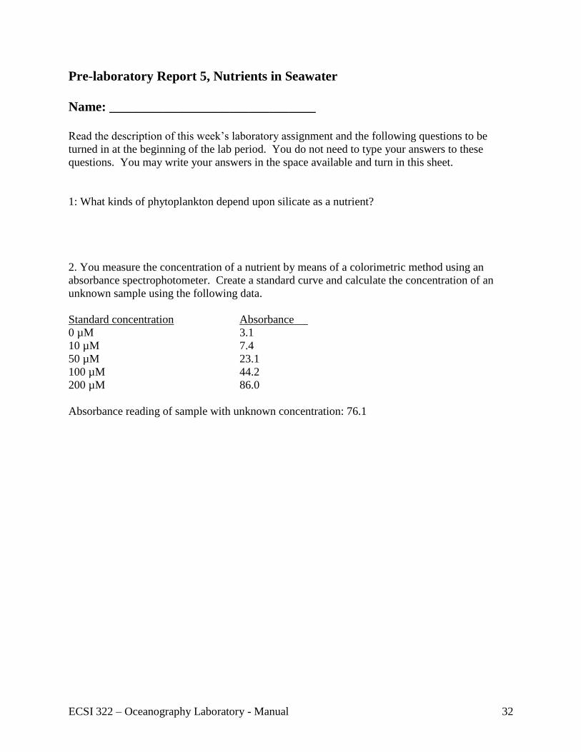
Pre-laboratory Report 5, Nutrients in Seawater
Name: _______________________________
Read the description of this week’s laboratory assignment and the following questions to be
turned in at the beginning of the lab period. You do not need to type your answers to these
questions. You may write your answers in the space available and turn in this sheet.
1: What kinds of phytoplankton depend upon silicate as a nutrient?
2. You measure the concentration of a nutrient by means of a colorimetric method using an
absorbance spectrophotometer. Create a standard curve and calculate the concentration of an
unknown sample using the following data.
Standard concentration Absorbance
0 µM 3.1
10 µM 7.4
50 µM 23.1
100 µM 44.2
200 µM 86.0
Absorbance reading of sample with unknown concentration: 76.1

ECSI 322 – Oceanography Laboratory - Manual 33
ESCI 322 Lab Report 3: Nutrients in Seawater
Objectives: The objective of this laboratory session is to learn standard techniques for the
analysis of dissolved ammonium and nitrate.
Broader learning objectives: Make a primary standard, a secondary standard, and a standard
curve. Learn precision pipetting. Learn the basics of colorimetric analysis of solutes. Observe
how an autoanalyzer works.
Nitrogen availability often limits productivity of coastal marine systems. Phosphorus can
sometimes be important too, especially in estuaries. Silica availability can limit abundance of
some groups that require silica, such as diatoms. We will obtain data on silicate, phosphate,
nitrate, and ammonium from samples we collected in Bellingham Bay. You will learn to
construct a standard curve for the calculation of nutrient concentrations in each of your samples;
after calculations are done, we will interpret the measured nutrient concentrations by discussing
sources and sinks of these substances. We will also examine the ratios of N and P in Bellingham
Bay and address the question whether concentrations of these nutrients follow Redfield ratios
(discussed below).
Most analytical methods for dissolved nutrient determination are colorimetric. Nutrients react
with reagents, producing colored compounds. The intensity of the color is quantified using a
spectrophotometer set at the appropriate wavelength. Color intensity is linearly related to the
amount of nutrient present. A standard curve allows us to relate the color intensity to the nutrient
concentration in the sample.
Part I: Nitrate (+ nitrite) and Ammonia
Concentrations of nutrients in marine waters are controlled by both the rate of nutrient input and
the rate of uptake by organisms. Phytoplankton take up nutrients in a consistent ratio, known as
the Redfield ratio. The Redfield ratio is the ratio in atoms of carbon, nitrogen, and phosphorus
assimilated by phytoplankton. This ratio is 106:16:1 (C:N:P). In addition, silicate often has a
1:1 ratio with phosphorus, depending upon the composition of the phytoplankton community.
Because concentrations of nutrients are so strongly tied to biological uptake, concentrations of
dissolved nutrients often follow this ratio. This week, by measuring nitrate + nitrite and
ammonium, the main inorganic nitrogen species in seawater, we can calculate the concentration
of total dissolved inorganic nitrogen ([DIN] = [NO3- + NO2
- + NH4+]) and compare it to the
concentrations of P and Si d (to be measured the following week) to determine whether
concentrations of nutrients in Bellingham Bay follow the Redfield ratio.
Analysis of dissolved Ammonium Outline of method (from Parsons et al. 1984): Seawater is treated in an alkaline citrate medium with
sodium hypochlorite and phenol in the presence of sodium nitroprusside which acts as a catalyser. The
blue indophenol color formed with ammonia is measured spectrophotometrically.
Procedures: Wear gloves and goggles. Make sure the spectrophotometer is turned on and set to a
wavelength of 640 nm. Set filter lever to the right. Set to 0% transmittance. Change mode to

ECSI 322 – Oceanography Laboratory - Manual 34
“absorbance”. Insert Nanopure water blank (this is not the same as the reagent blank). Set to 0%
absorbance.
Reagents: Reagents have also been made ahead of time. This procedure uses three: phenol solution,
sodium nitroferricyanide, alkaline reagent, sodium hypochlorite, oxidizing solution. These are
hazardous. Use caution and wear gloves and eye protection.
Phenol solution: 20g phenol in 200 ml 95% v/v ethanol
Sodium nitroferricyanide solution: 1 g sodium nitroferricyanide, in 200 ml D.I. H2O (Store in
dark glass bottle. Stable for one month.)
Alkaline reagent: 100 g sodium citrate and 5 g NaOH in 500 ml DI. H2O
Sodium hypchlorite solution: CloroxTM bleach (with no whiteners or additives)
Prepare oxidizing reagent: 100 ml alkaline reagent and 25 ml sodium hypochlorite solution (Chlorox).
Keep stoppered and prepare fresh daily. Ammonia standards Primary standards – 0.100 g ammonium sulphate (NH4)2SO4 in 1 L Nanopure water. Secondary standards – to be prepared from primary standards.
2° STD (M) L 1° STD/50 ml H2O 0.00 0 0.75 25 1.50 50 2.25 75 3.00 100 5.50 150
Quality control standard:
1.50 Procedure:
1. Pipette 5 ml aliquots of each secondary standard (2x for high standard), D.I. water blanks (2x), quality control standards (2x), and each sample (1x) into culture tubes
2. In fume hood, add 0.2 ml phenol, vortex, 0.2 ml nitroferricyanide, vortex, 0.5 ml oxidizing solution, vortex, and store in the dark for 1 h.
3. Vortex each sample and measure the absorbance at a wavelength of 640 nm in a spectrophotometer.
Calculations: The [NH4] of each sample is calculated as: [NH4] (M) = Sample absorbance - blank absorbance
Slope of standard curve (absorbance/M)
Analysis of dissolved nitrate
We will use an autoanalyser (Westco Smartchem) to analyze our samples for nitrate and nitrite. The
autoanalyser is perhaps the most common technology used for nutrient analysis in oceanography. This
allows large numbers of samples to be processed rapidly and high quality data can be produced by this
method.
Outline of method (from Parsons et al. 1984): Nitrate in seawater is reduced almost quantitatively to
nitrite when a sample is run through a column containing cadmium coated with metallic copper. The
nitrite produced is determined by diazotizing with sulfanilamide and coupling with N-(1-naphthyl)-

ECSI 322 – Oceanography Laboratory - Manual 35
ethylenediamine (NED) to form a highly colored azo dye which can be measured spectrophotometrically.
Any nitrite initially present in the sample must be corrected for, otherwise the result is reported as nitrate
+ nitrite.
Nitrate standards Primary standards – 10mM potassium nitrate solution. Dissolve 0.76 g potassium nitrate in 250 ml Nanopure water Refrigerate. (I'll prepare the nitrate standard ahead of time.) Reagents have also been made ahead of time. This procedure uses four: imidazole buffer, cupric sulfate
(0.01 M and 2%), sulfanilamide, and N-(1-naphthyl)-ethylenediamine (NED)
Imidazole buffer (0.1 M): Dissolve 3.40 g imidazole in 500 ml H2O. Dissolve imidazole in 400 ml H2O
in a beaker with a pH electrode and stirrer. Adjust solution to pH 7.0 with HCl. Transfer to 500 ml vol.
flask and dilute to mark. Refrigerate.
Cupric sulfate (0.01M): Dissolve 0.635 g cupric sulfate in 250 ml H2O. Stable.
Cupric sulfate (2% w/v): Dissolve 5 g cupric sulfate in 250 ml H2O. Stable.
Sulfanilamide: Slowly add 50 ml conc HCl to 350 ml H2O in 500 ml volumetric flask.
Dissolve 5 g sulfanilamide and dilute to mark. Stable.
NED: Dissolve 0.5 g NED in 500 ml H2O in volumetric flask. Refrigerate in brown bottle.
Pipette calibration Effects of temperature on fresh water density Temperature (°C) Density (g/ml)
10 0.9993
15 0.9977
20 0.9951
25 0.9914
27 0.9897
28 0.9888
30 0.9869
Prelaboratory report 6, Nutrients in seawater, due next week:
Calculate the concentrations of ammonium and nitrate (+ nitrite) in the samples we collected
from Bellingham Bay and Burrows Bay. Plot these data as profiles.

ECSI 322 – Oceanography Laboratory - Manual 36
ESCI 322 Lab Report 3, Nutrients in Seawater Part II - Phosphate and silicate
Objectives: Measure silicate and phosphate in our samples from Bellingham Bay.
Broader learning objectives: Learn how to create a truly zero blank using the reverse-addition
method. Learn how to interpret data on nutrients and other "non-conservative" tracers by
plotting the data versus salinity.
Analysis of dissolved silicate
Silicate is an important nutrient for diatoms and can be a limiting nutrient when nitrate and
phosphate are in high concentrations. Low concentrations of silicate relative to other nutrients
has been linked to shifts in phytoplankton species composition from diatoms to flagellates and
has been implicated in the formation of harmful dinoflagellate blooms.
Outline of method:
The seawater sample is allowed to react with molybdate under conditions which result in the
formation of silicomolybdate. A reducing solution, containing metol and oxalic acid, is then
added, which reduces the silicomolybdate complex to give a blue color and simultaneously
decomposes any phosphomolybdate and aresenomolybdate. The resulting extinction is measured
in a glass cuvette using a spectrophotometer at a wavelength of 810 nm.
Procedures:
Make sure the spectrophotometer is turned on and set to a wavelength of 810 nm. Set filter lever
to the right. Set to 0% transmittance. Change mode to “absorbance”. Insert Nanopure water
blank (this is not the same as the reagent blank). Set to 0% absorbance.
Use plastic (polypropylene) for everything. Glass is made of SiO2, the compound we are trying
to measure. In fact, the Earth's crust is ~60% SiO2. Consequently, contamination will be your
biggest obstacle to measuring silicate. Triple-rinse all labware just before use. Wear clean
gloves when handling samples, standards, and reagents. Keep your sample containers, standards,
and reagents free from dust.
Standards: To save time, we will use previously-made standards (5, 10, 20, 30, 40, and 50M
SIO4). Ordinarily, these would be made by dissolving Na2SiF6 in DIW.
Reagents: Reagents have also been made ahead of time. This procedure uses three: Metol-
sulfite reagent, oxalic acid, and sulfuric acid. These are hazardous. Use caution and wear
gloves and eye protection.
Procedure:
4. Pipette 2.5 ml of sample or standard into a clean 10-ml polypropylene centrifuge tube. 5. Add 1.0 ml of acidified ammonium molybdate reagent to each sample and standard. But
do not add this reagent to the blank [0M Si(OH)4]. Cap tightly and shake once or twice. The sample will now be at pH 1.0 - 1.5, and the following reaction will go to completion in about 10 minutes:

ECSI 322 – Oceanography Laboratory - Manual 37
Si(OH)4 + 12 MoO4= + 24 H+ -> H4SiMo12O40 + 12 H2O
(Silicomolybdic acid)
Wait at least 15 minutes before proceeding to the next step. This reaction forms a yellow compound (silicomolybdic acid), whose concentration is equal to that of the silicic acid initially present in the sample (1:1 stoichiometry). In samples with high [Si(OH)4] you will be able to see a pale yellow color form.
6. Mix reducing reagent: For each 2.5-ml sample to be analyzed mix 0.2 ml Metol-sulfite
reagent, 0.12 ml 10% oxalic acid, 0.12 m1 50% sulfuric acid and 0.16 ml DIW for a total volume of 3.1 ml. Use polypropylene graduated cylinders. First, rinse each cylinder twice with a few ml of Metol-sulfite reagent. Multiply these volumes by the number of samples to determine the total volume required for each reagent (see table below). Measure the reagents into a plastic beaker and cover with parafilm.
Reagent 1 sample 10 samples 20 samples 50 samples 100 samples
Metol-sulfite 0.5 ml 5 ml 10 ml 25 ml 50 ml
Oxalic Acid 0.3 ml 3 ml 6 ml 15 ml 30 ml
H2SO4 0.3 ml 3 ml 6 ml 15 ml 30 ml
DIW 0.4 ml 4 ml 8 ml 20 ml 40 ml
7. Add 1.5 ml of the mixed reducing reagent to all samples and standards. Cap tightly and shake once or-twice. Wait at least 2.5 hr for the yellow silicomolybdic acid to be reduced to a deep blue "silicomolybdous acid complex" - whose exact formula isn't known. In samples whose [Si(OH)4] is < ~1.5 M it will be difficult to see any color, but all others should be visibly blue. (If samples are not visibly blue, the waiting period can be reduced to 1.5 hr.)
While you are waiting for this reaction to occur, proceed to the phosphate measurements.
8. Now, add 1.0 ml of acidified ammonium molybdate reagent to the blank. This procedure
is called a reverse-addition blank. The oxalic acid in the mixed reducing agent blocks the formation of the yellow silicomolybdic acid so none forms when the acidified ammonium molybdate reagent is added later. This means the reverse-addition blank contains all the reagents and other colored compounds, but none of the blue-colored silica complex.
9. Measure the absorbance at a wavelength of 810 nm in a spectrophotometer (the blue
complex absorbs most strongly in the infrared), using glass culture tubes. We can use glass at this point because the silicate that we will measure has already formed the blue silicomolybdous acid complex and the oxalic acid blocks further complex formation.
Calculations: The [Si(OH)4] of each sample is calculated as:
[Si(OH)4] (M) = Sample absorbance - Reverse-addition blank absorbance Slope of standard curve (absorbance/M)
I will provide you with an excel spreadsheet that will help you make the appropriate calculations.

ECSI 322 – Oceanography Laboratory - Manual 38
Dissolved phosphate (H2PO4-, HPO4
2-, PO43-) determination (Parsons et al. 1984)
Phosphate is an important limiting nutrient in freshwater and marine systems. Eutrophication in
freshwater systems are often the result of high inputs of P, which lead to increased growth of
algae, and sometimes to reductions in dissolved oxygen or other problems. The importance of
phosphate for regulating the growth of algae was spectacularly demonstrated by Vollenweider
(1976). Figure 1 shows the relationship between total P loading and algal biomass in lakes.
Figure1. Empirical model relating mean surface chlorophyll-a concentrations of lakes to phosphorus
loading, adjusted for hydraulic loading. Plot from Cloern, 2001. Data from Vollenweider, 1976.
Outline of method:
The seawater sample is allowed to react with a reagent containing molybdic acid, ascorbic acid,
and trivalent antimony. The resulting complex is reduced to give a blue solution that is
measured at 885 nm.
Procedures:
Samples should be at room temperature. Turn on the spectrophotometer and set wavelength to
885 nm. This is the light absorption maximum for the blue solution produced in this method.
Standards: To save time we will make a set of working standards from a secondary standard that
has been prepared in advance. First a primary standard solution was made from anhydrous
KH2PO4 and DIW. The secondary standard was made from the primary standard.
Label and rinse five 100-ml volumetric flasks several times with DIW. Fill them with about 90
ml of DIW. Then, rinse an Erlenmeyer flask or beaker several times with a few ml of the
secondary standard solution. Using a volumetric pipette, carefully add the secondary standard
solution from the beaker to each 100-ml volumetric flask according to the table below. Bring up
the volume to 100 ml by carefully adding DIW. These are your tertiary standards.

ECSI 322 – Oceanography Laboratory - Manual 39
3° STD (µM) ml 2° STD / 100 ml H2O
0.0 0.00
0.6 0.50
1.8 1.50
3.0 2.50
4.2 3.50
Place six glass culture tubes in a tube rack (two for the blank and high standard) and record their
positions. Also add tubes for the seawater samples and record their positions.
Mixed reagent: We will create the mixed reagent from single reagents that were made in
advance of today’s lab.
For each 5-ml sample, use 0.1 ml Ammonium molybdate, 0.25 ml Sulfuric acid, 0.1 ml Ascorbic acid,
and 0.05 ml K-antimonyl-tartrate. First, wash a graduated cylinder with a few ml of ammonium
molybdate three times. Then, measure the correct volume of ammonium molybdate and the other
reagents according to the table below. Add these reagents to a labeled Erlenmeyer flask, cover with
parafilm, and mix for 30 seconds. Use volumes in the 50 samples column.
Reagent 10 samples 20 samples 50 samples
Ammonium molybdate 1.0 ml 2.0 ml 5.0 ml
Sulfuric acid 2.5 ml 5.0 ml 12.5 ml
Ascorbic acid 1.0 ml 2.0 ml 5.0 ml
K-antimonyl tartrate 0.5 ml 1.0 ml 2.5 ml
Measure 5 ml of each sample, each STD, and the nanopure H2O blank into culture tubes.
Add 0.5 ml mixed reagent. Wait 5 minutes. Measure absorbance on a spectrophotometer.
Spectrophotometric Procedures
Set the spectrophotometer at 885 nm. Turn spec on and allow to warm up for 15 min. Set
wavelength to 885 nm. Set filter lever to the right. Set to 0% transmittance. Change mode
to “absorbance”. Insert Nanopure water blank (this is not the same as the reagent blank). Set
to 0% absorbance. Insert sample and record absorbance.
Data Analysis for Phosphate
Follow the data analysis procedures for silicate.
Reporting nutrient concentrations in Bellingham Bay
The spatial distribution of temperature, salinity, and nutrients changes every time I sample Bellingham
Bay with students from this class. This is because we sample it at different stages of the tide and under
different wind conditions, and because the Nooksack River flow varies from year to year. One way to
make sense of the nutrient concentrations we measure, however, is to plot them versus salinity. This
enables us to examine the relationships between river input from the Nooksack, salt water input from the
Strait of Georgia and the Strait of Juan de Fuca, and nutrient concentrations within the bay without
reference to specific locations. We can even infer whether biological or chemical processes produce or
consume nutrients within Bellingham Bay as well. This method is described next.

ECSI 322 – Oceanography Laboratory - Manual 40
Understanding relationships between salinity and nutrient concentrations
Mixing theory: A non-reactive solute (sometimes referred to as a conservative tracer) supplied by a river
will be diluted by seawater. If dilution is the only process that determines the concentration of the
ttracer in an estuary, the relationship between tracer concentration and salinity will be linear. This also
holds for a tracer with a seawater input.
Figure 1. Theoretical
relationship between a
conservative solute and
salinity for solutes with (A)
a river source and (B) a
marine source.
A non-conservative tracer is one that has a source or sink within the estuary. In this case, the
relationship between tracer concentration and salinity will be non-linear.
Figure 2. Theoretical
relationships between non-
conservative solutes and
salinity for tracers with a
river source (A) and a marine
source (B).
By plotting nutrient concentrations versus salinity, we can infer whether the major sources or nutrients
to Bellingham Bay are from rivers or deeper, high salinity marine waters entering the bay at depth.
Deviations from a linear relationship indicate sources or sinks of N and P in the Bay. Like salinity, the
Redfield ratio can also be used to infer something about nutrient sources and sinks in Bellingham Bay.
If the DIN:DIP ratio deviates greatly from ~16, that would suggest a source or sink of N or P. Although
there are many processes that could cause nutrient concentrations to deviate from Redfield proportions,
the variation in this ratio with salinity can be used to learn something about nutrient cycling processes.
Salinity
Tra
cer
co
nce
ntr
ation
Salinity
Tra
cer
co
nce
ntr
ation
River source Marine sourceA B
Salinity
Tra
cer
co
nce
ntr
ation
Salinity
Tra
cer
co
nce
ntr
ation
River source Marine sourceA B
Salinity
Tra
cer
concentr
ation
Salinity
A B
Estuarine source
Estuarine sinkSalinity
Tra
cer
concentr
ation
Salinity
A B
Estuarine source
Estuarine sink

ECSI 322 – Oceanography Laboratory - Manual 41
Figure 3. Several processes that can cause nutrient
concentrations to deviate from Redfield proportions. (This
list is not complete.) Deviations at low salinity may reflect
river inputs. Phosphate-based fertilizers reduce the N:P ratio
whereas freshwater N fixation can increase it. Deviations at
high salinity in an estuary may reflect processes affecting
bottom waters. Denitrification in marine sediments can
reduce N:P whereas sorption of P onto sediments could
increase the ratio. Also, preferential uptake of N versus P in
the marine waters entering the bay could reduce N:P.
Creating a nutrient budget for Bellingham Bay: The data we have collected will allow us to
calculate a nutrient budget. This is a careful accounting of the rates of supply of nutrients from different
sources. The four potentially important sources that we can compare are: the Nooksack River, the Post
Point WWTP and deep water inflow from the Strait of Georgia/Strait of Juan de Fuca. Multiply the
nutrient concentrations in water from the Nooksack River, Post Point WWTP, and deep water with their
volumetric flow rates. Example: (15 mmole/m3 Nitrogen) * (7,000,000 m3/day Nooksack R. water) =
1.05*108 mmole/day nitrogen from the Nooksack River.
Create a budget for both nitrogen and phosphorus. You’ll need to calculate total nitrogen as the sum of
ammonium, nitrate and nitrite. Flow rates for the Nooksack River are available from the USGS. Flow
rates for the Post Point WWTP are available too. We can calculate the volumetric flow rate of deep
water from the Nooksack River flow rate and the extent to which Bellingham bay water is diluted using
the same methods as before: Ti = R[SO/(Si-SO)] = TO - R
Report: Our data on nutrient concentrations and salinity from various locations throughout Bellingham
Bay will allow us to ask the question: What are the sources and sinks of nutrients in Bellingham Bay?
To address this overall question, consider the following auxiliary questions. What is the relationship
between salinity and nutrient concentrations in Bellingham Bay? Is the Nooksack River an important
source of nutrients to Bellingham Bay or are higher salinity bottom waters more important? According
to your nutrient budget, which source is the most important? Are there other potential sources of
nutrients that we have overlooked? Are nutrients conservative tracers or do they have sources or sinks
in Bellingham Bay? Do nutrient concentrations in Bellingham Bay follow Redfield ratios? If not, what
does the deviation from Redfield proportions tell you about nutrient cycling in Bellingham Bay and
Puget Sound? Address these questions by plotting your data following Figures 1-3 (for each nutrient,
include all data from all stations), examine vertical profiles, and compare your data with theoretical
expectations. Present your nutrient budget as a table in your report including total inputs and % inputs.
References Cloern, J. E. 2004. Our evolving conceptual model of the coastal eutrophication problem. Mar. Ecol. Prog. Ser.
210, 223-253.
Parsons, T. R., Y. Maita, and C. M. Lalli. 1984. A manual of chemical and biological methods for seawater
analysis. Pergamon Press, Elmsford, N.Y.
Strickland, J. D. H. and T. R. Parsons. 1972. A Practical Handbook of Seawater Analysis. Fish. Res. Bd. Can. bull
167 . 2nd ed. pp 65-70.
Vollenweider, R. A. 1976. Advances in defining critical loading levels of phosphorus in lake eutrophication.
Mem. Ist. Ital. Idrobiol. 33, 53-83.
Salinity
DIN
:DIP
ratio
16
8
0
Redfield ratio
N < P:
Denitrification
In sediments?
N < P:
Fertilizer input?
N > P:
Nitrogen fixation?
N > P:
Phosphate storage
In sediments?
Salinity
DIN
:DIP
ratio
16
8
0
Redfield ratio
N < P:
Denitrification
In sediments?
N < P:
Fertilizer input?
N > P:
Nitrogen fixation?
N > P:
Phosphate storage
In sediments?
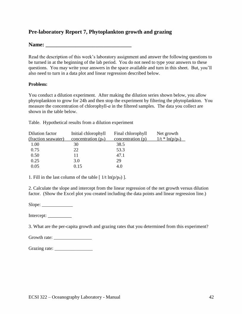
ECSI 322 – Oceanography Laboratory - Manual 42
Pre-laboratory Report 7, Phytoplankton growth and grazing
Name: _______________________________
Read the description of this week’s laboratory assignment and answer the following questions to
be turned in at the beginning of the lab period. You do not need to type your answers to these
questions. You may write your answers in the space available and turn in this sheet. But, you’ll
also need to turn in a data plot and linear regression described below.
Problem:
You conduct a dilution experiment. After making the dilution series shown below, you allow
phytoplankton to grow for 24h and then stop the experiment by filtering the phytoplankton. You
measure the concentration of chlorophyll-a in the filtered samples. The data you collect are
shown in the table below.
Table. Hypothetical results from a dilution experiment
Dilution factor Initial chlorophyll Final chlorophyll Net growth
(fraction seawater) concentration (p0) concentration (p) 1/t * ln(p/p0)
1.00 30 38.5
0.75 22 53.3
0.50 11 47.1
0.25 3.0 29
0.05 0.15 4.0
1. Fill in the last column of the table [ 1/t ln(p/p0) ].
2. Calculate the slope and intercept from the linear regression of the net growth versus dilution
factor. (Show the Excel plot you created including the data points and linear regression line.)
Slope: _____________
Intercept: __________
3. What are the per-capita growth and grazing rates that you determined from this experiment?
Growth rate: ________________
Grazing rate: ________________

ECSI 322 – Oceanography Laboratory - Manual 43
ESCI 322 Lab Report 4: Phytoplankton population growth and grazing
Objectives: Conduct a dilution experiment for estimating rates of population growth & grazing.
Broader learning objectives: Understand the mathematics and units of population growth and
grazing. Think about the role of grazers in controlling rates of phytoplankton growth.
Part 1: Setting up the experiment
The abundance of phytoplankton in the ocean is set by the balance between rates of population
growth, mortality and transport. Phytoplankton population growth rates in the field are affected
by light, nutrient concentration, temperature, and species composition among other factors.
Consumption by grazers is one of the largest sources of mortality. There are many grazers of
phytoplankton in Puget Sound; herring, calanoid copepods and bottom-dwelling filter feeders
such as clams are relatively large grazers. There are also phytoplankton grazers that are barely
larger than the phytoplankton cells they consume. These protistan grazers are termed
microzooplankton. In many marine ecosystems, microzooplankton are extremely important
phytoplankton consumers. The objective of this lab is to measure rates of phytoplankton growth
and microzooplankton grazing. We’ll perform the experiment at two light levels to better
understand how light and grazing interact to control phytoplankton abundance in the sea.
Theory: Consider the equation for population growth. It can be written in differential form as
follows: pdt
dp , where p is the concentration of phytoplankton and µ is the per-capita growth
rate. If z is the microzooplankton concentration and χ is the phytoplankton-zooplankton
encounter rate, you can add grazing to this equation as follows: zppdt
dp . Now, consider
what would happen if you diluted a sample of seawater with filtered seawater. Dilution should
not affect the growth rate of phytoplankton which multiply by binary fission. However, dilution
will reduce the encounter rate between phytoplankton and zooplankton, lowering the grazing
rate. If you add dilution (D is the fraction of undiluted seawater in the sample.) to the population
growth model, you can write it as gDppdt
dp , where g is the per capita mortality rate of
phytoplankton due to grazing. The solution to this model is p = p0e(µ-gD)t, where p0 is the initial
phytoplankton concentration. Taking the natural log of both sides and rearranging this equation
gives the following formula: gDp
p
t
0
ln1
. The first term is a measure of phytoplankton
net growth rate. Plotting this versus the dilution factor, D, yields a straight line with a slope
equal to g and intercept µ (Fig. 1). Thus, if you conduct a dilution experiment you can calculate
both the phytoplankton per capita growth and grazing rates. In our experiment, we will conduct
a dilution experiment with two light intensity treatments (full-strength light and 50% light).
We’ll use mesh screening material to manipulate light intensity and measure phytoplankton
growth and grazing rates at the two light levels. This will allow us to ask the question how does
phytoplankton growth respond to light and grazing?
Methods: It is a challenge to work with phytoplankton in late fall when biomass approaches its

ECSI 322 – Oceanography Laboratory - Manual 44
lowest levels due to low light levels. So, I will collect a big sample of seawater and let the algae
grow under well-lit conditions in the laboratory for a week prior to our class. That should give
us a sample with a high enough biomass to use for our experiment. Filter the water to create
three dilution levels – full-strength seawater, 50% seawater diluted with filtered seawater, and
10% seawater diluted with filtered seawater. Perhaps the trickiest part of setting up this
experiment will be filtering the water. You’ll need to filter a large quantity of water without
damaging the phytoplankton cells and then divide the seawater into replicate bottles while
keeping the cells in suspension so that all bottles receive the same concentration of cells. Filter
half the seawater through a filter cartridge using a peristaltic pump which won’t damage the
plankton. While filtering, use a piston to keep the cells in suspension. Then, combine the whole
and filtered seawater to create the following treatments, keeping the cells in suspension while
doing so.
Fraction whole Number of Light Sampling
Seawater replicates level time
100% 4 NA initial
100% 2 100% final
100% 2 10% final
50% 3 NA initial
50% 1 100% final
10% 4 NA initial
10% 2 100% final
10% 2 10% final
Incubate the samples for 48 hours. End the experiment by preserving a 15-ml sample from each
bottle using Lugol’s iodine preservative and pass the rest of the samples through a glass fiber
filter. Freeze the filters for analysis next week.
Figure 1. Theoretical relationship
between net growth rate and
dilution factor. The slope gives the
per capita grazing rate and the y
intercept gives the per capita
growth rate.
Reference: Landry, M.R., 2001. Microbial loops. In: Steele, J.H., Thorpe, S., Turekian, K.
(Eds.), Encyclopedia of Ocean Sciences, Academic Press, London, pp. 1763–1770.
Dilution experiments
Dilution factor (fraction SW)
Net
Gro
wth
Ra
te (
per
tim
e)
1
Decreasing # of Grazers
Y-intercept= “infinite dilution”
GROWTH RATE
Slope = linear relationship
with dilutions
HERBIVORY RATE
Growth equation: dp/dt = p – zp
dp/dt = p – zDp = p – gDp
Solution: 1/t ln(p(t)/p0) = – gD
0

ECSI 322 – Oceanography Laboratory - Manual 45
ESCI 322 Lab Report 4: Phytoplankton population growth and grazing
Week 2: Sample processing and analysis
Objective: Measure chlorophyll as a marker for phytoplankton biomass and estimate population
growth and grazing from the dilution experiment results. Identify phytoplankon groups
Broader learning objective: Learn to identify and enumerate phytoplankton. Also, observe
ciliate grazers from our experiment.
Reconsider the population growth equation that forms the basis of our dilution experiment:
gDp
p
t
0
ln1
. Note that ln(p/p0) is unitless. It depends on the ratio of p/p0 (the ratio of
final to initial phytoplankton concentration) and the units cancel. This means we can use any
measure of concentration we like to quantify the phytoplankton. The units don’t matter. We will
use chlorophyll concentration since it can be measured relatively easily and precisely. We will
also enumerate phytoplankton and microzooplankton cells to determine which species were most
strongly affected by grazers.
Review of chlorophyll measurement by fluorometry:
Chlorophylls absorb light energy at one wavelength and emit it a longer wavelength; this
property is known as fluorescence. Fluorescence measurements are quite sensitive so it can be
used to measure chlorophyll in dilute systems like ours. The fluorometer works by shining blue
light onto a pigment extract and measuring the resulting emission of red light. Filters are used to
control the wavelengths received by the sample and the detector (a photomultiplier tube). The
amount of blue light used to excite the fluorescence will influence the amount of fluorescence
produced; this is controlled by a series of “doors” and must be accounted for in the calculations.
The fluorometer is standardized using pure chlorophyll a extracts which in turn are quantified on
the spectrophotometer (this has been done for you). There are four steps involved in the
measurement of water column chlorophyll concentrations: i) filtering the water sample; ii)
grinding the filter (and attached particles) in acetone; iii) measuring the fluorescence of the
sample in a fluorometer; iv) calculating chlorophyll concentrations from fluorescence readings.
Step 1: Filtering the water sample
I have already filtered the samples and have frozen them for today’s analysis
Step 2: Sonicating the filter
a) Place a filter from step 1 into a 15-ml centrifuge tube and add 5 ml cold 90% acetone.
b) Sonicate while submerging the centrifuge tube in an ice-water bath for one minute. Wear
gloves, safety goggles and ear protection. c) When the sample is thoroughly sonicated, add acetone until the final volume is 10 ml.
d) Record the final volume of solvent plus homogenate in the tube. This is your “extraction
volume”. Put the tube into a test tube rack for storage in the ice bath (or freezer for longer-term
storage).

ECSI 322 – Oceanography Laboratory - Manual 46
Step 3: Measuring the sample fluorescence
a) Vortex or vigorously shake each centrifuge tube, then remove the filter, squeezing out any
solvent using a clean (solvent-rinsed) pair of forceps. Centrifuge the tubes (high speed, 5 min).
b) If extracts are visibly green, they must be diluted or the detector response will be saturated.
Use calibrated centrifuge tubes and automatic pipettes to dilute samples with 90% acetone; keep
track of all dilutions.
c) Zero the fluorometer using a cuvette containing 90% acetone. Re-zero every time you switch
door (sensitivity) settings.
d) Transfer your extract to a clean glass cuvette. Be careful not to resuspend any of the palletized
filter debris (this will interfere with the fluorescence reading).
e) Read the fluorescence of your extract. This value should be >25 and <95; the instrument
response is not linear outside this range. You will need to find the correct sensitivity setting for
use with each sample. (If the reading is off-scale on the 1x setting, you will need to dilute your
extract; see step 1, above.) Record sample name, volume of water or culture filtered, volume of
acetone used for extraction, and the fluorescence reading, including the sensitivity setting.
f) Without removing cuvette from fluorometer, add 2 drops of 1 N HCl. Record the fluorescence
after the reading stabilizes. Do not change the sensitivity setting, even if the new reading is <25.
Rinse cuvette well (3x) with 90% acetone to remove any acid.
Step 4: Calculating the chlorophyll concentration
Calculate chlorophyll concentration in each water sample using the following equations (from
Lorenzen, 1966):
Chl a (µg/liter seawater) =)1(
)(0
mf
amx
Fv
dFFvFK
Phaeopigments (µg/liter seawater) =)1(
)(0
mf
ammx
Fv
dFFFvFK
where:
Fo = fluorescence before acidification
Fa = fluorescence after acidification
Fm = maximum acid ratio which can be expected in the absence of pheopigments ≈ 2.2
Kx = calibration factor for a specific sensitivity scale units: [(µg Chl a/ml solvent)/instrument
fluorescence unit]
k1x = 7.12 x 10⁻⁴, k3x = 2.40 x 10⁻⁴, k10x = 6.43 x 10⁻⁵, k30x = 2.48 x 10⁻⁵
v = volume of acetone used for extraction (ml)
vf = volume of seawater filtered (liters)
d = extract dilution factor (e.g. if you diluted 1 ml extract by adding it to 4 ml solvent, your
dilution factor would be 5. If no dilution, d = 1).
Note that most of these factors reduce to a constant for a given set of instrument calibration
factors. I will post a spreadsheet containing these formulas for your convenience.
Determining cell densities:
Determine the density of phytoplankton and microzooplankton in your samples by counting them
with a Sedgwick Rafter counting slide. This slide holds exactly 1 ml of sample. The 10-ml

ECSI 322 – Oceanography Laboratory - Manual 47
samples were preserved with Lugol’s iodine solution in 15-ml centrifuge tubes.
Before counting the samples, perform a tenfold cell concentration step. Centrifuge the samples
and, using a glass pasture pipette, carefully remove the top 9 ml of solution leaving just under 1
ml in the tube. Then, transfer the remaining solution into the Sedgwick rafter cell. Do this by
placing the slide cover on top of the cell at an angle leaving two small triangular openings on
each side of the cell. Dispense your sample into one of these openings and fill the cell. If the
sample does not fill the entire cell, add some distilled water. Once the cell is filled, twist the
cover slip to enclose the sample. To count the sample, place the counting cell on a compound
microscope. Start on one corner of the slide and count “lanes” that cross the entire cell. At the
end of each lane, move the slide the width of one field of view and count the next adjacent lane.
Repeat until you’ve covered the entire slide. Record the number and types of plankton you
observe. Count approximately 300 individual plankters in each sample. Calculate the percent
abundance of each type of alga.
Report
Calculate the per-capita growth and grazing rates for each treatment. Your report should address
the following questions: How important is grazing in controlling phytoplankton growth? How
might the relationship between light intensity, growth and grazing influence the vertical
distribution of phytoplankton biomass?
Reference
Lorenzen, C. J. 1966. Determination of chlorophyll and pheo-pigments: spectrophotometric
equations. Limnol. Oceanogr. 12: 343-346.