Un i ve r s i t y o f He i de l b e r g

Discussion Paper Series No. 428

Department of Economics

Environmental problems and economic development in an endogenous fertility model

Frank Jöst, Martin Quaasand Johannes Schiller

August 2006

Environmental problems and economic development

in an endogenous fertility model ∗

Frank Josta, Martin F. Quaasb, Johannes Schillerc

Abstract. Population growth is often viewed as a most oppressive global problem with

respect to environmental deterioration, but the relationships between population devel-

opment, economic dynamics and environmental pollution are complex due to various

feedback mechanisms. We analyze society’s economic decisions on birth rates, invest-

ment into human and physical capital, and polluting emissions within an optimal control

model of the coupled demographic-economic-environmental system.

We show that a long-run steady state is optimal that is characterized by a stable

pollution stock, and by population and economic growth rates depending on the possibil-

ities of emission abatement and technical progress due to human capital accumulation.

We derive a condition on the production technologies and opportunity costs of raising

children, under which the optimal birth rate is constant even during the transition to a

steady state. In particular in an economy where only human capital is needed to produce

output, the optimal choice of the birth rate is not affected by the states of the economy or

the environment. In such a setting, the optimal birth rate is constant and policy should

concentrate on intertemporal adjustment of per-capita emissions.

JEL-Classification: Q56, J10, O13

Keywords: Sustainability, Economic Development, Endogenous Fertility

∗The authors thank Dale Adams, Clive Bell, Malte Faber, J.A. Smulders and Till Requate for helpful

comments on earlier drafts.

aCorresponding author. Alfred-Weber-Institute of Economics, University of Heidelberg, Grabengasse

14, D-69117 Heidelberg, Germany. email: frank.joest@uni-hd.de

bDepartment of Ecological Modelling, UFZ–Centre for Environmental Research Leipzig-Halle, Ger-

many. email: martin.quaas@ufz.de

cDepartment of Economics, UFZ-Centre for Environmental Research Leipzig-Halle, Germany. email:

johannes.schiller@ufz.de

1 Introduction

In the 2001 report “Footprints and Milestones: Population and Environmental Change”,

the United Nations Population Fund states that changes in demographic variables such

as size, growth rates or distribution of population have an important impact on the

environment. However, there are feedback mechanisms between population and envi-

ronmental change and the relationship between environmental quality and population is

complex. The amount and type of emissions are not only determined by demographic

variables, but also depend on production technologies and consumption patterns. Hence,

even a growing population does not necessarily lead to an increasing deterioration of

environmental quality. If e.g. highly polluting consumption is substituted by goods of

less polluting character, or technical progress and investments in human capital occur,

overall environmental quality may improve even with an increasing population. Further-

more, one has to take into account that the development of the natural environment, the

economy and even the number of children is mainly driven by decisions of people, which

respond to changes of economic and environmental conditions. Taking this into account,

the analysis of the relationship between demographic change, economic development and

environmental deterioration should include the following characteristics:

• People decide on the number of their children, i.e. fertility is endogenous.

• Output is mainly produced by industrial production systems with emissions as un-

wanted by-products which may accumulate in the surrounding natural environment.

• Industrial production processes are characterized by the possibility to mitigate emis-

sions, by the use of physical and human capital, which allows for an increase in

output with the same amount of emissions.

• Environmental deterioration is caused by the stock of pollutants which stem from

industrial production.

The existing economic literature on the relationship between population and the environ-

ment analyses the above mentioned characteristics only partially. Most of the contribu-

tions describe a situation typical for rural areas in less developed countries. These areas

are characterized by small agricultural production units, in which usually even young

2

children contribute to the output of a family, e.g. by collecting firewood or looking after

cows. Therefore households feel an incentive to have more children in order to achieve a

higher output. However, additional children have an impact on the output of other fami-

lies which is not part of the individual decision making of families. Dasgupta (1993, 2000)

and Shah (1998) analyze these population externalities in static models. A similar, but

dynamic model structure is explored by Nerlove (1991) and Nerlove and Mayer (1997).

However, they do not primarily analyze population externalities, but put their main em-

phasis on the analysis of conditions for a stationary state in which environmental quality

and population are constant.

Models which are more appropriate for the situation of a country with industrial pro-

duction have been developed by Cronshaw and Requate (1997), Harford (1997, 1998) and

Shou (2002). Using a static model with exogenous fertility, Cronshaw and Requate (1997)

analyze the impact of population growth on the environment and production applying

comparative-static methods. Harford (1998) investigates pollution and population exter-

nalities within a dynamic model with endogenous fertility, but he neglects the production

side of the economy. Shou (2002) presents a dynamic model with endogenous fertility

and human capital in order to analyze pollution externalities, but considers only flow

pollution and neglects physical capital as a production input.

It is the aim of our contribution to integrate the above mentioned characteristics of

the relationship between population, the economy and the environment. For this sake we

extend existing models in the environmental economic literature referred to in the last

paragraph. In particular, the starting point of our analysis is an endogenous economic

growth model with stock pollutants (for an overview of this literature see Xepapadeas 2003

or Smulders 2000). We extend this model by using elements from the literature on

endogenous fertility and economic growth (a comprehensive survey is given by Nerlove

and Raut 1997).1

In particular, we assume that population growth and environmental deterioration

are the results of the decisions of households with respect to consumption, pollution

and the number of children. Concerning population dynamics, we abstract from age

1Since we are primarily interested in the analysis of environmental problems, we neglect the liter-

ature on resource problems and population growth. For this strand of literature see e.g. Kogel and

Prskawetz (2001).

3

structure and assume mortality to be exogenous. The environment is modelled as a

stock of pollutants degrading environmental quality. The economic system is modelled

using an approach based on a physical as well as human capital stock. The model is

formulated as an optimal control model in order to get insights into the characteristics

of the optimal development of the economic-environmental-demographic system, taking

into account that the production of goods causes environmental damage and that this

damage negatively influences the utility of present and future generations.

In particular, we are interested in the following aspects:

1. We show under what conditions a steady state exists in our model framework and

we analyze the characteristics of such a long-run optimal development of the cou-

pled economic-environmental-demographic system. In particular, we investigate the

conditions on the society’s preferences, technical abatement possibilities and techni-

cal progress due to human capital accumulation under which a growing population

and consumption are optimal in the long run.

2. We are interested in the characteristics of the transition paths to the long-run

equilibrium, because the environmental subsystem and the population subsystem

change slowly in comparison to changes in the economy. This leads to a complex

transition dynamics. In addition, a detailed analysis of the transition path allows

us to identify conditions, under which we can assume that the development of a

subsystem is exogenously given. Given the fact that in the environmental eco-

nomics literature there are only few papers, which assume that population growth

is endogenous, we clarify under which conditions fertility should be endogenous and

under which conditions population development can reasonably be assumed to be

exogenously given. We show that the answer to these questions crucially depends on

the relative importance of physical and human capital in the production of goods.

3. We discuss the implication of our results for the design of environmental and pop-

ulation policy.

The paper is organized as follows. In section 2, we develop the intertemporal optimization

model, and we present the first- and second-order conditions in section 3. Section 4

discusses the characteristics of the steady state and presents some comparative static

4

results. In section 5, we analyze the dynamics of the transition towards the steady state.

We derive conditions under which population can be assumed to be exogenous. We

furthermore analyze two special cases of the model: one where no physical capital is used

in production and one where only physical capital, but no human capital is used. We

show that the former case exhibits fairly simple transitional dynamics, while the latter

includes the relevant dynamic interrelations between the three subsystems, which prevail

in the full model. We therefore perform the detailed analysis of the transition dynamics

for the simpler model without human capital. Finally, section 6 summarizes our results

and discusses some implications for environmental and population policy.

2 Model

Our modeling approach is to consider the optimal development of a coupled system com-

prising the three subsystems population, natural environment and production of goods.

The dynamics of the subsystems is described by characteristic stock variables and corre-

sponding control variables. The control variable corresponding to the population stock

N(t) (at time t) is the gross birth rate n(t). The stock of pollutant S(t), which describes

the state of the environment, is controlled by per capita emissions e(t). Concerning the

production system, we consider two stocks: per capita physical capital k(t), which is

controlled by per capita consumption c(t); and per capita human capital h(t), which is

controlled by the share l(t) of human capital employed in goods production. (For the

sake of a concise notation, we will omit the explicit time dependence of these variables

in the following and write N instead of N(t) etc.)

2.1 The social planner

In our modeling approach, we assume that a central planner chooses the time path of the

four control variables in order to maximize intertemporal welfare. Aggregate intertem-

poral welfare can be measured either in terms of the sum of utility of all individuals or

in terms of the average, i.e. per capita, utility. With endogenous population both ap-

proaches lead to different outcomes (for an overview on this issue see Razin and Sadka

1995). In our model, we follow the same approach as Harford (1997, 1998), and employ

5

per capita utility to measure social welfare. The welfare functional is given by the present

value of an infinite per capita utility stream

U =

∞∫0

u (c, n,N, h, S) exp(−ρ t) dt, (2.1)

where ρ > 0 is the constant discount rate, and u (c, n,N, h, S) is the instantaneous utility

function of a representative individual.

The per capita instantaneous utility function is concave and increases in consumption

per capita c and in the birth rate n, reflecting the fact that parents enjoy having children.

It also increases in the population size N , which accounts for possible positive effects of

an overall larger population size on utility (e.g. due to altruism of parents towards their

adult children, Becker and Barro 1988). Furthermore, it rises with the level h of human

capital in the model economy. This captures that individual utility is higher, the higher

the own education is, and, since h is also the children’s human capital (see below), it also

captures that parents are interested in the ‘quality’ of their children (Becker et al. 1999).

Finally, per capita utility decreases in the pollutant stock S.

In order to keep our model simple, we use the following log-linear instantaneous

utility function.2

u(c, n,N, h, S) = ln c+ ν lnn+ ω lnN + η lnh+ σ lnQ(S), (2.2)

where Q(S) with Q′(S) < 0 measures environmental quality. In proposition 3 and

lemma 2, we will furthermore assume the functional form Q(S) = exp(−S), which

corresponds to an instantaneous utility function with constant marginal damage from

pollution. In equation (2.2), ν, ω, η, and σ are strictly positive constants.

2.2 Population

Neglecting the age structure and assuming an exogenous constant death rate d, the

dynamics of population growth are described by the following equation, where the dot-

2It is possible, though tedious, to show that most of results also hold for the more general Cobb-

Douglas utility function

u(c, n,N, h, S) =(c nν Nω hη Q(S)σ)1−θ

1− θ.

6

superscript denotes a time-derivative.3

N = (n− d)N . (2.3)

We treat N and n as continuous variables. This approximation is valid because we

exclusively regard large numbers for population size N . Hence, n denotes an average

birth rate. With the same rational, instead of regarding an individual’s probability to

die, we employ an average death rate d for the whole population.

2.3 Environment

To describe the accumulation of polluting emissions in the environment and the natural

degradation of pollution in a very simple way, we assume the following equation of motion

for the pollutant stock.

S = N e− δ S . (2.4)

Here, we disregard any spatial heterogeneity of the pollution problem and assume that

the pollutant is equally distributed throughout the environment. δ denotes the natural

degradation rate of the pollutant and is assumed to be constant. Hence, pollution degra-

dation is proportional to the concentration of the pollutant in the environmental system.

For example, this assumption is reasonable for the greenhouse gas CO2 if one exclusively

considers the anthropogenic CO2 excess above the natural level. Furthermore, this excess

has to be comparatively small and timescales regarded must not be too long.4

2.4 Production

Each of the N individuals is endowed with human capital h. We consider three options,

how the human capital can be used: for production of goods, for raising children, or

3Of course, the assumption of a constant death rate is unrealistic. In particular, as Chu and Yu (2002)

discuss there is a lot of evidence that the death rate depends on the the state of the environment. However,

this problem is not the main focus of our paper. Hence we assume a constant death rate, which helps to

simplify our analysis.

4For a critical comment on the use of a single differential equation for the description of the accumu-

lation of greenhouse gases in the environment see Joos, Muller-Furstenberger and Stephan (1999) and

Moslener and Requate (2001).

7

for accumulating new human capital. We denote the share of human capital employed

in production with l. In order to raise and educate one child, a fraction φ of human

capital is needed at the instant, at which the child is born (this approach follows Yip and

Zhang 1997 and Barro and Sala-I-Martin 1995). Thereafter, this child is endowed with

the average human capital stock h. Given the birth rate n, the share of human capital

needed to raise and educate all newly born children is φn. Since this fraction of human

capital cannot be used for production of goods nor for accumulating new human capital,

opportunity costs of raising children occur, which increase with the level of human capital.

A share 1− l− φn of human capital remains for accumulating human capital. Following

Lucas (1988), we assume a linear technology of human capital accumulation, which is

given by the equation

h = ψ · (1− l − φn) · h . (2.5)

This means that each unit of human capital can generate ψ ≥ 0 additional units of human

capital (the case ψ = 0 is considered in section 5.3, otherwise we assume ψ > 0). Since

we disregard depreciation of human capital, it cannot decrease, i.e. h ≥ 0. Including a

constant depreciation rate would be straightforward, but complicate notation.

The production output consists of a homogeneous good, which can either be con-

sumed directly or invested into the stock of physical capital. Disregarding depreciation of

physical capital, and denoting per capita output with y, the accumulation of per capita

physical capital is governed by the following equation:

k = y − c− (n− d) k . (2.6)

Since n − d is the growth rate of population (cf. equation 2.3), the term −(n − d) k

expresses the fact that each new member of the population has to be provided with the

per capita amount of capital for k to remain constant.

In addition to the desired output y, production of goods generates emissions e as

unwanted joint outputs. These emissions can be abated. This requires an increased input

of the other inputs, physical and human capital. Formally, emissions can be treated as

an input into the production process, which can be substituted by other input factors

(Siebert 1998).5 The production technology is described by the following Cobb-Douglas

5In real production systems, however, the ‘substitution’ of emissions by other inputs is time consum-

ing.

8

production function which gives output per capita as a function of the production inputs,

physical capital k, the share l of human capital h spent for production of goods, l h, and

emissions e.

y = f(k, l h, e) ≡ kα1 (l h)α2 eα3 , (2.7)

where α1 ≥ 0, α2 ≥ 0 and α3 > 0. We assume decreasing returns to scale in per capita

output, i.e. α1 +α2 +α3 < 1. This assumption, which is required for an interior optimum,

does not exclude endogenous growth, as we show below.

In addition to the full model, two special cases with regard to the production side

will be considered: in section 5.2, we consider the case α1 = 0, i.e. production without

physical capital; and in section 5.3, we consider the case α2 = 0 and ψ = 0, i.e. production

without human capital.

3 Conditions for the optimal development

The optimal development of the coupled demographic-economic-environmental system is

derived from the maximization of the intertemporal welfare function (2.1) subject to the

four restrictions (2.3), (2.4), (2.5) and (2.6). In order to solve the maximization problem

we define the current value Hamiltonian

H(k, c, λk h, l, λh, N, n, λN , S, e, λS) =

u(c, n,N, h, S) + λk (f(k, l h, e)− c− (n− d) k) + λh ψ (1− l − φn) h

+ λN (n− d)N + λS (N e− δ S) . (3.1)

We get the first order conditions (FOC) for an optimum by taking the derivatives with

respect to control (i.e. c, l, n, e) and state (i.e. k, h,N, S) variables. Denoting a derivative

with respect to one of the control or state variables by the corresponding subscript, we

obtain the following equations:

Hc = 0 uc − λk = 0 (3.2)

Hl = 0 λk fl − λh ψ h = 0 (3.3)

Hn = 0 un − k λk − λh ψ φh+ λN N = 0 (3.4)

He = 0 λk fe + λS N = 0 (3.5)

9

Hk = ρ λk − λk λk (fk − (n− d)) = ρ λk − λk (3.6)

Hh = ρ λh − λh uh + λk fh + λh ψ (1− l − φn) = ρ λh − λh (3.7)

HN = ρ λN − λN uN + λN (n− d) + λS e = ρ λN − λN (3.8)

HS = ρ λS − λS uS − λS δ = ρ λS − λS (3.9)

In addition, the transversality condition requires

limt→∞

λx x = 0 for all stocks x ∈ {k, h,N, S} . (3.10)

The first order conditions (3.2) to (3.9) together with the transversality conditions (3.10)

are sufficient for an optimum, if the maximized Hamiltonian, which is the Hamiltonian

evaluated at the optimum given by the first order conditions, is concave in the state

variables (Arrow and Kurz 1970:48).

We show in appendix A that the maximized Hamiltonian is not necessarily concave

in our model, due to the endogenous choice of the birth rate.6 However, we also derive

conditions, under which the maximized Hamiltonian is concave.7 In the following analysis,

we assume that these conditions hold, such that the first order conditions (3.2) to (3.9)

and (3.10) determine the optimum.

As we are interested in the optimal time paths of the four control variables, c, l, n,

and e, we eliminate the co-state variables λk, λh, λN , and λS from equations (3.2) to

(3.9). This leads to the following set of differential equations (see appendix B).

1

uc

ducdt

= ρ− [fk − (n− d)] (3.11)

1

uc fl

d(uc fl)

dt= ρ− ψ h

[uc fhuc fl

+uhuc fl

](3.12)

1

uc fe

d(uc fe)

dt= ρ−

[N usuc fe

− (n− d)− δ

]. (3.13)

Equation (3.11) is the familiar Ramsey-condition for optimal consumption in the case of

non-constant population: the growth rate of marginal utility from consumption equals

6Problems concerning the existence of solutions or the sufficiency conditions in models with endoge-

nous fertility are extensively discussed by Razin and Sadka (1995) and Schweizer (1996).

7In particular, these conditions require the assumptions of (i) decreasing returns to scale in per capita

output, (ii) a positive weight of population in the utility function, and (iii) a positive weight of human

capital in the utility function, which have been made in section 2.

10

the discount rate minus the effective rate of return to physical capital. Concerning equa-

tion (3.12), the expression uc fl can be interpreted as the marginal utility of the share

of human capital employed in production of the consumption good. In the optimum, its

growth rate equals the discount rate minus the effective rate of return on investing human

capital in human capital accumulation. This effective rate of return consists of two parts:

first, investment into human capital generates increased (future) output of consumption

goods and second, it generates utility due to a higher education level. Interpreting the

left hand side of equation (3.13) as the marginal utility of per capita emissions, its growth

rate equals the discount rate minus an effective ‘rate of return’ on the pollutant stock,

which consists of three terms: first, the marginal damage (per capita) from aggregated

emissions, second, the population growth rate, which corrects for aggregate rather than

per capita effects (as in the Ramsey-condition) and third, the increase δ in depreciation

of an increased pollution stock.

At this point, we will skip the derivation of a corresponding equation that determines

the dynamics of the birth rate. We come back to this issue in section 5. Inserting the

functional forms (2.2) of the instantaneous utility function and (2.7) of the production

function into equations (3.11), (3.12) and (3.13) leads to the following explicit equations

of motion for the three controls c, l, and e (see appendix B)

c

c= fk − ρ− (n− d) (3.14)

l

l=−(1− α3)A− α3B + α1

kk

+ α2hh− c

c

1− α2 − α3

(3.15)

e

e=−α2A− (1− α2)B + α1

kk

+ α2hh− c

c

1− α2 − α3

(3.16)

with

A ≡ 1

fl uc

d(fl uc)

dt= ρ− ψ l − ψ η

α2

c l

f(3.17)

and

B ≡ 1

fe uc

d(fe uc)

dt= ρ+ δ + n− d+

σ

α3

N eQ′(S)

Q(S)

c

f. (3.18)

We analyze the optimal development of the model in two steps: in the following section 4,

we study the long-run steady state dynamics, while the focus of section 5 is on the

11

transitional dynamics from any given initial state of the model economy to the steady

state.

4 Steady state analysis

In this section, we derive the steady state dynamics of the model and give some economic

interpretations. Let gc, gl, gn, ge, gk, gh, gN , gS be the constant, but possibly different,

growth rates of the endogenous quantities in the steady state. The equations of motion

of the four stock variables N (equation 2.3), S (equation 2.4), k (equation 2.6), and h

(equation 2.5) are rearranged in order to get the conditions for the growth rates in the

steady state.

gN ≡N

N= n− d (4.1)

gS ≡S

S=

N e

S− δ (4.2)

gk ≡k

k= k−(1−α1) (l h)α2 eα3 − c/k − (n− d) (4.3)

gh ≡h

h= ψ (1− l − φn) . (4.4)

Given these growth rates, the following lemma is derived immediately.

Lemma 1

In a steady state,

1. the birth rate and the share of human capital employed in goods production are

constant, i.e. gn = 0 and gl = 0;

2. the growth rate of the pollutant stock equals the sum of the growth rates of popu-

lation and per capita emissions, i.e. gS = gN + ge.

Proof: See appendix C.1.

Part 1 of the lemma states the following: in order to achieve stable steady state

population dynamics, per capita birth rates have to be constant, which stems from the

constant death rate d. Given the linear technology of human capital accumulation (equa-

tion 2.5), i.e. that the growth rate of human capital is proportional to the share of human

capital employed in human capital accumulation, it is clear that this share has to be

12

constant in a steady state. Hence, since the share of human capital spent for raising

children is constant in a steady state, also the third share of human capital, l, which is

employed in the production of goods, is constant. Part 2 of the lemma states that in the

long-run equilibrium dynamics, the growth rate of the pollutant stock equals the growth

rate of aggregate emissions. Given lemma 1, we derive the remaining steady-state growth

rates.

Proposition 1

Given the utility function (2.2) and the production function (2.7), the growth rates in

the steady state are gl = gn = 0 (by lemma 1) and

gS = 0 (4.5)

ge = −gN (4.6)

gc = gk =α2

1− α1

gh +α3

1− α1

ge . (4.7)

Proof: see appendix C.2.

The steady state for our model is characterized by a constant optimal long run pol-

lution stock, i.e. its growth rate gS is zero. Pollution can not grow exponentially without

bound, due to increasing marginal damages. Neither is it optimal to have decreasing

immissions in the long run, because emissions would have to decrease exponentially, too,

which would cut consumption possibilities too severely. The pollutant stock can only be

constant, if total emissions N e are constant, too (cf. equation (4.2)). This implies that

the growth rate of total population and per capita emissions are equal in absolute value,

but of opposite sign (lemma 1).

The sign of the population growth rate, however, depends on the difference between

the optimal birth rate and the exogenously given death rate. The optimal birth rate, in

turn, depends on the exact parameter constellation (see propositions 2, 3, and 4 below).

Hence, whether population is growing or declining in the long-run optimum is not clear

in the first place. If the optimal growth rate of population is positive, the per capita

emissions decline in the long run optimum and vice versa. With a stationary population,

i.e. gN = 0, per capita emissions also have to be constant, i.e. ge = 0.

Proposition 1 contains the familiar result that the optimal growth of per capita

consumption is equal to the growth rate of per capita physical capital. In addition, both

growth rates are equal to the weighted sum of the growth rate of human capital and

13

emissions (cf. equation 4.7), which is due to the Cobb-Douglas form of the production

function (2.7). Since per capita emissions grow at a rate which equals the negative

growth rate of population, per capita consumption grows at a rate, which is equal to the

weighted sum of the human capital growth rate and the population growth rate, i.e. gc =

α2/(1−α1) gh−α3/(1−α1) gN . Because the weights are always positive the growth of per

capita consumption depends negatively on the growth rate of population and positively on

the growth rate of human capital. Hence, a growing population does not necessarily lead

to a declining per capita consumption, since this negative effect could be offset by growth

in human capital. Since human capital growth is non-negative in our model, per capita

consumption will not decline in the steady state, unless population is growing at a high

rate. This is due to the Cobb-Douglas production function, which admits substitution

between the polluting emissions and man-made capital at a comparatively high elasticity

of substitution (see Dasgupta and Heal 1979).

5 Transition dynamics

In this section, we focus on questions related to the transitional dynamics of the system.

First, we derive conditions, under which population is growing at a constant rate even

during the transition to the steady state. Second, we investigate the characteristic features

of the control paths in the transitional dynamics towards the steady state for two special

cases: in section 5.2, we consider a model economy which produces without physical

capital,8 in section 5.3, we consider an economy, where no human capital is used in

production. We perform the detailed analysis of the transitional dynamics for this simpler

model rather than for the full model including human capital, in order to be able to derive

some analytical results.

5.1 Conditions for constant optimal population growth

Addressing the first question, we derive the equation of motion for the optimal choice

of the birth rate n, which corresponds to the equations of motion for the other control

8The case without physical capital is considered e.g. by Schou (2002) in a model with flow pollution.

14

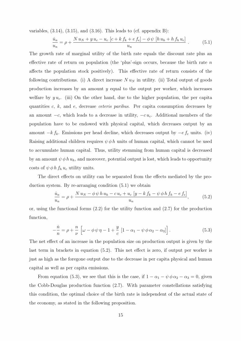
variables, (3.14), (3.15), and (3.16). This leads to (cf. appendix B):

unun

= ρ+N uN + y uc − uc [c+ k fk + e fe]− φψ [huh + h fh uc]

un. (5.1)

The growth rate of marginal utility of the birth rate equals the discount rate plus an

effective rate of return on population (the ‘plus’-sign occurs, because the birth rate n

affects the population stock positively). This effective rate of return consists of the

following contributions. (i) A direct increase N uN in utility. (ii) Total output of goods

production increases by an amount y equal to the output per worker, which increases

welfare by y uc. (iii) On the other hand, due to the higher population, the per capita

quantities c, k, and e, decrease ceteris paribus. Per capita consumption decreases by

an amount −c, which leads to a decrease in utility, −c uc. Additional members of the

population have to be endowed with physical capital, which decreases output by an

amount −k fk. Emissions per head decline, which decreases output by −e fe units. (iv)

Raising additional children requires ψ φh units of human capital, which cannot be used

to accumulate human capital. Thus, utility stemming from human capital is decreased

by an amount ψ φhuh, and moreover, potential output is lost, which leads to opportunity

costs of ψ φh fh uc utility units.

The direct effects on utility can be separated from the effects mediated by the pro-

duction system. By re-arranging condition (5.1) we obtain

unun

= ρ+N uN − φψ huh − c uc + uc [y − k fk − ψ φh fh − e fe]

un, (5.2)

or, using the functional forms (2.2) for the utility function and (2.7) for the production

function,

− nn

= ρ+n

ν

[ω − φψ η − 1 +

y

c[1− α1 − ψ φα2 − α3]

]. (5.3)

The net effect of an increase in the population size on production output is given by the

last term in brackets in equation (5.2). This net effect is zero, if output per worker is

just as high as the foregone output due to the decrease in per capita physical and human

capital as well as per capita emissions.

From equation (5.3), we see that this is the case, if 1 − α1 − ψ φα2 − α3 = 0, given

the Cobb-Douglas production function (2.7). With parameter constellations satisfying

this condition, the optimal choice of the birth rate is independent of the actual state of

the economy, as stated in the following proposition.

15

Proposition 2

If the net effect of a change in the population size on production output is zero, i.e.

α1 + ψ φα2 + α3 = 1, (5.4)

the optimal birth rate n? is constant and given by

n? =ρ ν

1 + ψ φ η − ω. (5.5)

Proof: See appendix C.3.

Proposition 2 can be interpreted as following. In the ‘technologies’ of production of

goods, accumulating human capital and educating children satisfy condition (5.4), the

various feedback effects between the optimal birth rate, the economy’s development and

environmental pollution cancel out. Hence, under these conditions the choice of the birth

rate is not affected by the dynamics of the other subsystems. Rather, it depends solely

on exogenous quantities. Because the death rate is also exogenous, the growth rate of

population equals n? − d and is constant over time. If condition (5.4) is met, our model

with endogenous fertility therefore yields a constant optimal population growth, which is

fully determined by exogenous parameters.

Condition (5.4), however, is restrictive. It may only be fulfilled, if the opportunity

costs (in terms of foregone human capital accumulation and output) of raising children

are high. Since 1−α1−α2−α3 > 0, condition (5.4) requires in particular ψ φ > 1, more

specifically,

ψ φ = 1 +1− α1 − α2 − α3

α2

. (5.4’)

If raising children requires even more human capital, the effect of an increased population

on net output is negative. If it requires less human capital, the effect of an increased

population on net output is positive. In both cases, the optimal choice of the birth

rate depends on the state of the economy, in particular on the share of output, which is

consumed, c/y. This quantity, in turn, depends on the values of the four stock variables.

Thus, the birth rate will in general not be constant over time, if condition (5.4) is not

met.

The way in which the different parameters influence the birth rate given by equa-

tion (5.5) is plausible: the optimal birth rate increases with the relative weights ν of

children as well as ω of population in the utility function (2.2). It decreases with the

16

opportunity costs of raising children, ψ φ η, which arise because having children implies

less human capital accumulation and, hence, less utility stemming from human capital

endowment.

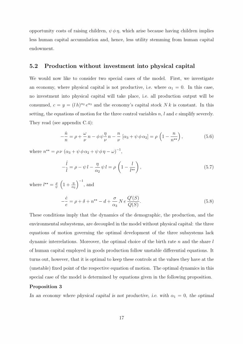
5.2 Production without investment into physical capital

We would now like to consider two special cases of the model. First, we investigate

an economy, where physical capital is not productive, i.e. where α1 = 0. In this case,

no investment into physical capital will take place, i.e. all production output will be

consumed, c = y = (l h)α2 eα3 and the economy’s capital stock N k is constant. In this

setting, the equations of motion for the three control variables n, l and e simplify severely.

They read (see appendix C.4):

− nn

= ρ+ω

νn− φψ

η

νn− n

ν[α3 + ψ φα2] = ρ

(1− n

n??

), (5.6)

where n?? = ρ ν (α3 + ψ φα2 + ψ φ η − ω)−1,

− ll

= ρ− ψ l − η

α2

ψ l = ρ

(1− l

l??

), (5.7)

where l?? = ρψ

(1 + η

α2

)−1

, and

− ee

= ρ+ δ + n?? − d+σ

α3

N eQ′(S)

Q(S). (5.8)

These conditions imply that the dynamics of the demographic, the production, and the

environmental subsystems, are decoupled in the model without physical capital: the three

equations of motion governing the optimal development of the three subsystems lack

dynamic interrelations. Moreover, the optimal choice of the birth rate n and the share l

of human capital employed in goods production follow unstable differential equations. It

turns out, however, that it is optimal to keep these controls at the values they have at the

(unstable) fixed point of the respective equation of motion. The optimal dynamics in this

special case of the model is determined by equations given in the following proposition.

Proposition 3

In an economy where physical capital is not productive, i.e. with α1 = 0, the optimal

17

birth rate and the optimal share of human capital employed in production are constant,

n = n?? =ρ ν

α3 + ψ φα2 + ψ φ η − ω, (5.9)

l = l?? =ρ

ψ

(1 +

η

α2

)−1

. (5.10)

If furthermore Q(S) = exp(−S), i.e. marginal damage from pollution is constant, the

optimal control path of emissions is given by

e =α3 (ρ+ δ)

σ N=

α3 (ρ+ δ)

σ N0 exp((n?? − d) t). (5.11)

Proof: See appendix C.4.

Whereas in the full model, a rather specific condition on the parameters is required

to obtain a constant birth rate in the transition to the steady state, the birth rate is

always constant in the model, in which no physical capital is employed in production.

The reason for this result is that each person consumes the output it produces, since no

investment in physical capital is required. Hence, the net effect of a higher birth rate on

per capita output is always zero. (Remember that this was the condition for a constant

birth rate in proposition 2.)

In contrast to the constant birth rate derived in equation (5.5) of proposition 2 for

the case in which the production effects of a change in the birth rate cancel out, there

are two additional terms in the denominator of equation (5.9). They capture the effect

of the birth rate on the production side of the economy, namely α3 and ψ φα2. The

different parameters affect the birth rate in a plausible way: the higher the exponent α3

of emissions in the production function and the higher the opportunity costs of raising

children in terms of foregone output (ψ φα2), the lower is the optimal birth rate.

Proposition 3 implies that two of the controls, i.e. the share of human capital em-

ployed in production, and the birth rate, are constant and that the third control, the per

capita emissions, is adjusted over time such as to obtain constant aggregate emissions N e

(cf. equation 5.11).

Thereby, since the birth rate is fixed at a given level, per capita emissions have to

be adjusted to the growing (or declining) population over time. In other words, in order

to control the environmental quality optimally, the population development is treated

as exogenous, while per capita emissions are adjusted. Because aggregate emissions N e

18

are constant, the pollutant stock exponentially decays or increases to its steady state

value (cf. equation 2.4), depending on the initial conditions. If Q(S) 6= exp(−S), i.e.

for increasing rather than constant marginal damages of pollution, most of the results of

proposition 3 remain valid, except for the constant aggregate emissions (equation 5.11),

which depend on the pollutant stock in that case.

5.3 Production without investment into human capital

We now consider the other special case, an economy where human capital is not produc-

tive, neither in production of goods, i.e. α2 = 0, nor in accumulating human capital, i.e.

ψ = 0. In this case, the conditions of proposition 2 cannot be fulfilled within our frame of

analysis – we require α1+α3 < 1 in order to come up with a concave Hamiltonian. Hence,

it will generally not be optimal to choose a constant birth rate during the transition to

the steady state. Correspondingly, in a model which does not comprise human capital

the birth rate has to be endogenous in order to find the optimal solution. We have a true

interrelation between the choices of the birth rate, consumption and polluting emissions.

In contrast to the special case, where human capital is productive, but physical capital

is not, we thus find non-trivial transition dynamics towards the steady state. Before we

turn to the analysis of the transition dynamics, we characterize the steady state for this

special case of the model.

Proposition 4

1. Given the utility function (2.2) and production without human capital, the optimal

growth rates in the steady state are gS = 0, ge = −gN and

gc = gk =α3

1− α1

ge. (5.12)

2. If the conditionρ ν

α1 + α3 − ω= d (5.13)

is met, then n??? = d. As a consequence, the steady state is a stationary state, in which

all quantities are constant, i.e. gc = gk = ge = gS = gN = n??? − d = 0.

Proof: See appendix C.5.

Without human capital there is no long-run economic growth in the model – per

capita consumption can only increase if population shrinks. A constant level of per

19

capita consumption is however possible for a constant population size.9

If the parameters fulfill condition (5.13), the steady state birth rate is given by the

left hand side of this condition. It has a similar form as in the settings of propositions 2

and 3: the steady state birth rate increases ceteris paribus with rising weight ν of children

and ω of population in the utility function, and it decreases with the output elasticities

of the two production factors capital, α1, and emissions, α3.

Our first step in analyzing the optimal dynamics of the model without human capital

is to linearize the system of the equations of motion (these are the equations (C.55) –

(C.59), given in appendix C.5) in the neighborhood of the steady state. The dynamics of

this linearized system is described by the Jacobian matrix evaluated at the steady state.

In particular, the absolute values of the negative eigenvalues of this Jacobian matrix

may be interpreted as time scales of the optimal dynamics of the coupled demographic-

economic-environmental system (this interpretation is justified in appendix C.6). The

eigenvalues are given by the following lemma.

Lemma 2

Given the utility function (2.2), production without human capital, constant marginal en-

vironmental damages (i.e. Q(S) = exp(−S)) and if the parameters fulfill condition (5.13)

(i.e. population is constant in the steady state), the Jacobian matrix in the steady state

has the eigenvalues

µ1 = −δ (5.14)

µ2 =ρ

2

1−

√√√√1 +4

1− α3

[1− α1

α1

− ν

(1− α1 − α3

α1 + α3 − ω

)2] (5.15)

µ3 = 0 (5.16)

µ4 = ρ (5.17)

µ5 =ρ

2

1 +

√√√√1 +4

1− α3

[1− α1

α1

− ν

(1− α1 − α3

α1 + α3 − ω

)2] (5.18)

µ6 = ρ+ δ . (5.19)

Proof: See appendix C.6.

9In a model without human capital, but with exogenous, Harrod-neutral technical progress, per capita

consumption could increase even with a growing population, provided, the rate of technical progress is

sufficiently high (Jost et al. 2004).

20

According to lemma 2, the Jacobian matrix has one eigenvalue equal to zero, µ3;

three positive eigenvalues (or with positive real parts, in case µ5 is a complex number),

µ4, µ5, and µ6; one negative eigenvalue, µ1; and one eigenvalue, µ2, which may either be

negative or positive.

With the interpretation of the absolute values of the negative eigenvalues as time

scales of the optimal dynamics of the coupled system, we can now analyze how the dy-

namic behavior of the coupled system changes, if parameters change, without knowing the

exact solution of the dynamic system. This is done by investigating how the parameters

describing the internal dynamics of the subsystems affect the timescales of the coupled

system. In addition, we can analyze, how parameter changes affect the stability proper-

ties of the optimal path by checking whether they change the signs of the eigenvalues.

The results are given in the following proposition.

Proposition 5

Under the assumptions of lemma 2, parameter changes have the following consequences

for the optimal dynamics of the model economy:

1. Assuming µ2 < 0, if the natural deterioration rate δ of the pollutant stock or the

discount rate ρ increase, the steady state is approached more rapidly.

2. Assuming µ2 < 0, an increase of the output elasticity of physical capital, α1 ac-

celerates the optimal dynamics of the coupled system for small α1 and retards the

dynamics for large values of α1.

3. If the preferences for children, ν, or population, ω, increase, a shift in the stability

properties of the optimal path can occur.

Proof: See appendix C.7.

Parts 2 and 3 of this proposition point out, that the model of economic development

and stock pollution with endogenous fertility exhibits some complexity in the optimal

dynamics. It is not clear, how parameter changes (in particular changes in the output

elasticity of physical capital) affect the optimal dynamics, nor are global statements

possible about the stability properties of the optimal path.

In order to derive some qualitative properties of the optimal path in the transition

to the steady state, we show a numerical example, which is calculated using a dynamic

21

programming technique. The details of the simulation and the parameters are described

in appendix D. The parameters and starting values of the stock variables were chosen

for illustrative reasons; a calibration of the model to realistic values is beyond the scope

of this paper. The assumed parameters fulfill condition (5.13), such that the population

size is constant in the steady state, n??? = d, and are chosen such that µ2 < 0. The

results of the simulation are shown in figure 1.

Every optimal path is characterized by six time-dependent variables: N , k, S, n, c

and e. Thus, the phase space has six dimensions. The left column of Figure 1 shows the

optimal path for the specified set of parameters and initial stocks in three projections

of the phase space into the planes spanned by the stock variables N , k and S and their

corresponding control variables n, c and e. The right column of Figure 1 shows the time

paths of all six variables. The simulation was over 130 time steps; after 50 time steps,

the steady state is approximately reached.

As expected, the birth rate is not constant during the transition period: it declines

monotonically over time to its steady state value. Accordingly, the population size in-

creases quickly in the beginning and then approaches a constant steady state value. The

projection of the optimal path to the population-birth rate-plane is a monotonically de-

clining curve. Per capita consumption is comparatively low in the beginning, allowing for

investment into physical capital, and rises gradually to its constant steady state value,

where also the per capita capital stock is constant.

Particularly interesting are the characteristics of the optimal path concerning emis-

sions and the pollution stock: the initial value of the pollution stock was chosen to be

0.85, which is above the steady state value S??? = 0.5. In the very beginning, there is

a sharp increase in the polluting stock, resulting from a very high emission level.10 This

is due to the stability properties of the optimal path.11 A continuous optimal control

path does not exist for arbitrary initial values of the three stock variables N , k and S.

In particular, such a continuous path does not exist for the initial stocks chosen in the

10e(t = 1) = 0.16, far above the remaining values.

11The (6× 6) Jacobian matrix of the linearized system of equations of motion at the steady state has

only two negative eigenvalues. Given the parameters in Table 1, these eigenvalues are −0.245, −0.154,

0, 0.1, 0.254, 0.345. Hence, the stable sub-space is only two-dimensional rather than three-dimensional,

which would be required for a saddlepoint-stable optimal path.

22

population N

birt

hra

ten

1.251.21.151.11.0510.950.90.850.8

0.09

0.08

0.07

0.06

0.05

0.04

0.03

time t

birth rate n

50403020100

0.09

0.08

0.07

0.06

0.05

0.04

time t

population N

50403020100

1.2

1.1

1

0.9

per capita capital stock k

per

capi

taco

nsum

ptio

nc

43.532.521.51

1.3

1.2

1.1

1

0.9

0.8

0.7

0.6

time t

p.c. consumption c

50403020100

1.3

1.2

1.1

1

0.9

0.8

0.7

0.6

time t

p.c. capital k

50403020100

4

3.5

3

2.5

2

1.5

1

pollutant stock S

per

capi

taem

issi

onse

10.90.80.70.60.50.4

0.048

0.046

0.044

0.042

0.04

0.038

0.036

time t

p.c. emissions e

50403020100

0.046

0.044

0.042

0.04

0.038

0.036

time t

pollution stock S

50403020100

0.9

0.8

0.7

0.6

0.5

Figure 1: The figure shows the optimal path for the set of parameters given in Table 1

and initial stocks k(0) = 1, N(0) = 0.85, and S(0) = 0.85. On the left hand side in three

projections of the phase space; on the right, the time path of every variable is depicted,

each cross indicating a time step. A discontinuous jump in the controls occurs in the first

time step due to the lack of (saddlepoint-)stability of the optimal path.

23

example. In this case it is optimal to choose extreme values for the control variables

initially in order to reach the optimal path, which is pursued continuously afterwards.

This is obtained by choosing very high per capita emissions as well as comparatively high

per capita consumption and a large birth rate in the very beginning.

A further characteristic feature of the optimal dynamics is illustrated by Figure 1:

the optimal control path is in general non-monotonic in at least one of the controls. This

means that (in this example) per capita emissions have to be drastically reduced first,

then are allowed to increase for a certain period of time and finally have to be reduced

again in order to approach the steady state.

6 Conclusions

The interrelation between environment, population development and economic growth is

a complex issue due to the mutual interdependencies. The same holds for the dynamic

properties of our model. Nevertheless, our analysis leads to some clear-cut results.

A long-run steady state is optimal within the framework of our model and is char-

acterized by constant population growth (or decline), economic growth (or contraction)

and a stable pollution stock. The birth rate in the steady-state depends on parameters of

all subsystems. In particular, whether it exceeds the death rate, i.e. whether population

grows, declines, or is constant in the long-run optimum, depends not only on the valu-

ation of children, but also on the production technology and in particular on emission

abatement possibilities. Long-run per consumption growth is only possible by means

of continued accumulation of human capital, which is a ‘clean’ substitute for polluting

inputs. More specifically, unless human capital per capita is growing faster than popula-

tion, the output elasticity of human capital must exceed the output elasticity of emissions

in order to have long-run growth in per capita consumption.

Since both, the demographic and the environmental subsystems are driven by slow

time scales, the transition towards a steady state requires a long time compared to usual

economic time scales. Thus, the transition dynamics is of particular importance in this

context, and we devoted a large part of the analysis on this.

We have shown that in a special case, where no physical capital is used in produc-

tion, the transition dynamics is very simple: except for per capita emissions, the control

24

variables are constant over time. This implies that the three subsystems are de-coupled,

and that there are no interdependencies between the population and the environment,

which could be termed ‘complex’. Of course, one has to be cautious with far reaching

conclusions on the basis of such a simple model. But this result suggests that in an

economy where physical capital is of minor importance in production as compared to

human capital, the interrelations between demographic development, economic growth

and environmental deterioration are not too complex. In particular, it is not necessary

to adapt population policy to the state of the environment or the dynamic development

of the economy. Rather, per capita emissions have to be adapted over time and should

therefore have the primary political attention.

However, in most cases, it seems more realistic that physical capital is important for

the production of consumption goods. Then, how each of the subsystems is optimally

controlled at a given instant in time depends not only on its own current state but also

on the current states of the other subsystems. In general a non-monotonic time path of

the control variables is necessary in order to achieve the steady state, i.e. controls must

not simply be de- or increased, but the direction in which they are adapted has to be

changed at some point in time. This, of course, is a challenging policy advice.

Only under a specific constellation of production technology and children’s education,

the demographic subsystem is decoupled from the other subsystems, and the birth rate

is constant even during the transition towards a steady state. This is the case, if the

output, which would be produced by a new child, is just as high as the output which

is would be lost, because this new child (i) needs human capital to be educated, (ii)

has to be endowed with physical capital and (iii) generates additional need for abating

emissions. More technically speaking, the condition given in proposition 2 on the output-

elasticities of the factors of production and the opportunity costs of raising children has to

be fulfilled. From a theoretical point of view, it is not necessary to include an endogenous

birth rate into a dynamic model of population, economy and environmental deterioration

if this condition is met.

25

References

Arrow, K. and M. Kurz (1970). ‘Public Investment, The Rate of Return, and Opti-

mal Fiscal Policy’, Published for Resources for the Future, John Hopkins Press,

Baltimore.

Barro, R.J. and X. Sala-I-Martin (1995). ‘Economic Growth’, McGraw-Hill, New York.

Becker, G.S. and R.J. Barro (1988). ‘A Reformulation of the Economic Theory of

Fertility’, Quarterly Journal of Economics, 103(1):1-25.

Becker, G.S., E.S. Glaeser, and K.M. Murphy (1999). ‘Population and Economic

Growth, AEA Papers and Proceedings, 89(2):145-149.

Chu, C. Y. C. and R. R. Yu (2002). ‘Population Dynamics and the Decline in Biodiver-

sity: A Survey of the Literature’, Population and Development Review, 28(0):126–

143.

Dasgupta, P. and G. M. Heal (1979). Economic Theory and Exhaustible Resources,

Cambridge University Press, Cambridge.

Dasgupta, P. (1993). An Inquiry into Well-Being and Destitution, Clarendon Press,

Oxford.

Dasgupta, P. (2000). ‘Population and Resources: An Exploration of Reproductive and

Environmental Externalities’, Population and Development Review, 26(4):643–689.

Ehrlich, P.R. and A.E. Ehrlich (1990). ‘The Population Explosion’, New York.

Galor, O. and D.N. Weil (2000). ‘Population, Technology, and Growth: From Malthu-

sian Stagnation to the Demography Transition and Beyond’, American Economic

Review, 90(4):806–828.

Harford, J.D. (1997). ‘Stock Pollution, Child-Bearing Externalities, and the Social

Discount Rate’, Journal of Environmental Economics and Management, 33:94-105.

Harford, J.D. (1998). ‘The ultimate externality’, American Economic Review, 88(1):269-

265.

26

Jost, F., M. Quaas and J. Schiller (2004). ‘Population growth and environmental dete-

rioration: an intertemporal perspective’, Discussion paper No. 400, Department of

Economics, University of Heidelberg.

Joos, F., G. Muller-Furstenberger and G. Stephan (1999). ‘Correcting the carbon cycle

representation: how important is it for the economics of climate change’, Environ-

mental Modeling Assessment, 4:133-140.

Keeler, E., M. Spence and R. Zeckhauser (1971). ‘The optimal control of pollution’,

Journal of Economic Theory, 4:19-34.

Kogel, T. and A. Prskawetz (2001). ‘Agricultural productivity growth and escape from

the Mathusian trap’, Journal of Economic Growth, 6:337-357.

Lucas, R.E. (1988). ‘On the Mechanics of Development Planning’, Journal of Monetary

Economics, 22:3–42.

Moslener, U., T. Requate (2001). ‘Optimal Abatement Strategies for Various Inter-

acting Greenhouse Gases - Is the Global Warming Potential a Useful Indicator?’,

Discussion Paper No. 360, Economics Department, University of Heidelberg.

Nerlove, M. (1991). ‘Population and the environment: a parable of firewood and other

tales’, American Journal of Agricultural Economics, 73:1334-1347.

Nerlove, M. and A. Meyer (1997). ‘Endogenous fertility and the environment: a parable

of firewood’, in: Dasgupta, P., K.G. M”aler (ed.) The Environment and Emerging

Development Issues, Vol. 2, Clarendon Press, Oxford:259-282.

Nerlove, M., A. Razin and E. Sadka (1987). ‘Household and Economy. Welfare Eco-

nomics of Endogenous Fertility’, Academic Press, Boston.

Nerlove, M. and L.K. Raut (1997). ‘Growth models with endogenous population: a

general framework’, in: Rosenzweig, M. R., Stark, O. (eds.), Handbook of Population

and Family Economics, Vol. 1 B, Elsevier, Amsterdam:117-1174.

Razin A., E. Sadka (1995). Population Economics, MIT Press, Cambridge, Massachusetts.

27

Robinson, J. A. and T.N. Srinivasan (1997). ‘Long-term consequences of population

growth: technological change, natural resources, and the environment’, in: Rosen-

zweig, M. R., Stark, O. (eds.), Handbook of Population and Family Economics, Vol.

1 B, Elsevier, Amsterdam:1175-1298.

Schou, P. (2002). ‘Pollution Externalities in a Model of Endogenous Fertility and

Growth’, International Tax and Public Finance, 9:709-725.

Schweizer, U. (1996). ‘Endogenous fertility and the Henry George theorem’, Journal of

Public Economics, 61:209-228.

Shah, A. (1998). Ecology and the Crisis of Overpopulation. Future Prospects for Global

Sustainability, Edward Elgar, Cheltenham, UK.

Siebert, H.(1998). Economics of the Environment. Theory and Policy, 5th revised

edition, Springer-Verlag, Heidelberg.

Smulders, S. (2000). ‘Economic Growth and Environmental Quality’, in: Folmer, H.

and Gabel, K. (eds.), Principles of Environmental Economics, Edward Elgar, Chel-

tenham.

UN-ICPD (1994). Programme of Action of the UN International Conference of Popu-

lation and Development, Cairo.

Xepapadeas, A. (2003). ‘Economic Growth and the Environment’, in: Maler, K-G.

and Vincent, J. (eds.), Handbook of Environmental Economics, Vol. 3, Elsevier,

Amsterdam (forthcoming).

Yip, Ch.K. and J. Zhang (1997). ‘A simple endogenous growth model with endogenous

fertility: indeterminacy and uniqueness’, Journal of Population Economics, 10:97-

110.

28

Appendix

A Sufficient conditions

We derive the sufficient conditions for the optimum considering the specification (2.2) for the

utility function (with Q(S) = S − S, the case Q(S) = exp(−S) is analogous), and (2.7) for the

production function.

The first order conditions are also sufficient if the maximized Hamiltonian H0 is quasi-

concave in the state variables (Arrow, Kurz 1970).12 This is the case, if the Hessian is negative-

semidefinite, i.e. if (cf. Mas-Colell et al. 1995:935-940)

H0kk ≤ 0 (A.1)∣∣∣∣∣∣ H

0kk H0

kh

H0hk H0

hh

∣∣∣∣∣∣ ≥ 0 (A.2)

∣∣∣∣∣∣∣∣∣H0kk H0

kh H0kN

H0hk H0

hh H0hN

H0Nk H0

Nh H0NN

∣∣∣∣∣∣∣∣∣ ≤ 0 (A.3)

H0SS ≤ 0. (A.4)

The first condition holds, if

H0kk = λk

d

dk[fk − n] = λk

d fkdk

− dn?

dk(A.5)

From (3.4), dn?/dk = −n?2/ν λk. From equations (3.3) and (3.5),

1l

? dl?

dk=

α1

1− α2 − α3

1k

(A.6)

1e

? de?

dk=

α1

1− α2 − α3

1k

(A.7)

Using into (A.5) leads to

H0kk = λk

d fkdk

− λkdn?

dk= λk fk

[−1− α1

k+α2

l?dl?

dk+α3

l

? de?

dk

]− λk

dn?

dk

= − 1k2

[λk k fk

1− α1 − α2 − α3

1− α2 − α3− (n? λk k)2

ν

](A.8)

Hence, condition (A.1) is fulfilled, if

fk1− α1 − α2 − α3

1− α2 − α3≥ n?2 λk k

ν(A.9)

12The maximized Hamiltonian H0 is the function H after we have substituted the control variables by

the optimal values determined by conditions (3.2)-(3.5).

29

This is only possible, if α1 + α2 + α3 < 1.

Next, we turn to condition (A.2). The relevant second order derivatives of the maximized

Hamiltonian are

H0hh = − η

h2+

d

dh

=0︷ ︸︸ ︷[λk fh − λh ψ l

]−φλh dn

?

dh= − η

h2− ψ φλh

dn?

dh

= − 1h2

[η − (ψ φn? λh h)2

ν

]. (A.10)

From (3.4), dn?/dh = −ψ φn?2/ν λh. From equations (3.3) and (3.5),

1l

? dl?

dh= −1

h(A.11)

1e

? de?

dh= 0. (A.12)

Hence,

H0hk = λk

d

dh[fk − n?] = λk

[f − k

[α2

h+α2

l?dl?

dh+α3

e?de?

dh

]− dn?

dh

]=

1k h

λk k λh hφψ n?2

ν(A.13)

Condition (A.2) leads to the following requirement, which is obtained by inserting (A.8), (A.10),

and (A.13) into (A.2)

η λk k fk1− α1 − α2 − α3

1− α2 − α3≥ λk k fk

1− α1 − α2 − α3

1− α2 − α3

(λh hφψ n?

)2

ν+ η

(λh hφψ n?

)2

ν.

(A.14)

This condition requires η > 0.

From equation (3.2), dc?/dN = 0, from (3.4), dn?/dN = n?2/ν λN .

H0NN =

d

dN

[ ωN

+ λN n? + λS e?]

(A.15)

= − ω

N2+ λN

dn?

dN+ λS

de?

dN(A.16)

= − 1N2

[ω − 1

ν(n? λN N)2 − λk e fe

1− α2

1− α2 − α3

](A.17)

Because, from (3.3), (1− α2) 1/l? dl?/dN = α3 1/e? de?/dN . In equation (3.5):

uc fe

[α2

1l?dl?

dN− (1− α3)

1e?de?

dN

]+ λS = 0 (A.18)

⇔ de?

dN= − e?

N

1− α2

1− α2 − α3(A.19)

dl?

dN= − l?

N

α3

1− α2 − α3(A.20)

30

H0kN = λk

d

dN[fk − n?] = − 1

N k

[α1 α2 λ

k f

1− α2 − α3+λk k λN N n?2

ν

](A.21)

H0hN = λN

dn?

dh+ λS

de?

dh= − 1

N h

λN N λh hφψ n?2

ν(A.22)

condition (A.3) requires

H0kH0

hhH0NN + 2H0

hN H0hkH0

kN

≤ H0hh

[H0kN

]2 +H0kk

[H0hN

]2 +H0NN

[H0kh

]2 (A.23)

This condition can only be fulfilled, if d2H0/dN2 < 0, which, in turn, requires ω > 0 (equa-

tion (A.17)).

Finally, condition (A.4) is fulfilled for the given specifications of Q(S), because

H0SS = − σ

(S − S)2. (A.24)

B Derivation of the equations of motion

The first order conditions (3.2)–(3.9) are rewritten as follows:

λk = uc (B.25)

λh h =1ψfl uc (B.26)

un = − λN N + λk k + ψ φλh h (B.27)

−λS =uc feN

(B.28)

uc (fk − ρ− (n− d)) = − d

dtλk (B.29)

huh + uc h fh − uc flρ

ψ= − d

dt

(λh h

)(B.30)

N uN − uc e fe − ρ λN N = − d

dt

(λN N

)(B.31)

uS − (δ + ρ) λS = − λS (B.32)

Using conditions (B.25), (B.26) and (B.28) into (B.29), (B.30), and (B.32), respectively, with

slight rearrangement, leads to the set of differential equations (3.11), (3.12), and (3.13).

Using the utility function (2.2) and the production function (2.7) into equations (3.11),

(3.12) and (3.13), respectively, leads to

k

k− c

c= ρ+

f

k− c

k− fk (B.33)

α1k

k− (1− α2)

l

l+ α2

h

h+ α3

e

e− c

c= ρ− ψ l − ψ η

α2

c l

f(B.34)

α1k

k+ α2

h

h+ α2

l

l− (1− α3)

e

e− c

c= ρ+ δ + n− d+

σ

α3N e

Q′(S)Q(S)

c

f(B.35)

31

Using

k

k=

f

k− c

k− (n− d) (B.36)

h

h= ψ (1− l − φn), (B.37)

we havec

c= fk − ρ− (n− d) (B.38)

Rearranging equations (B.34) and (B.35) leads to

−(1− α2)l

l+ α3

e

e= A− α1

k

k− α2

h

h+c

c(B.39)

α2l

l− (1− α3)

e

e= B − α1

k

k− α2

h

h+c

c(B.40)

where

A ≡ ρ− ψ l − ψ η

α2

c l

fand (B.41)

B ≡ ρ+ δ + n− d+σ

α3N e

Q′(S)Q(S)

c

f(B.42)

Solving for l/l and e/e yields

−(1− α2 − α3)l

l= (1− α3)A+ α3B − α1

k

k− α2

h

h+c

c(B.43)

−(1− α2 − α3)e

e= α2A+ (1− α2)B − α1

k

k− α2

h

h+c

c(B.44)

Next, we derive a corresponding equation for the optimal choice of the birth rate n. We therefore

differentiate condition (B.27) with respect to time:

un = − d

dt

(λN N

)+d

dt

(λk k

)+ ψ φ

d

dt

(λh h

)(B.45)

Using (B.29), (B.30), and (B.31) leads to

un = N uN −uc e fe− ρ λN N −uc (k fk − ρ k − f + c)−ψ φ[huh + uc h fh − uc fl

ρ

ψ

](B.46)

Using λN N from condition (3.8) and rearranging leads to equation (5.1).

C Proofs of lemmas and propositions

C.1 Proof of lemma 1

Ad 1. gn = 0 follows from (4.1) with gN!= 0. Using this in (4.4) leads to gl = 0. Part 2 is

proved by differentiating (4.2) w.r.t. time.2

32

C.2 Proof of proposition 1

We start with the derivation of the equations gk = α2/(1− α1) gh − α3/(1− α1) gN .

Differentiating equation (3.14) with respect to time, using gc = 0 in the steady state and

n? = l? = 0 (lemma 1), leads to

fk = 0 ⇒ −(1− α1)k

k+ α2

h

h+ α3

e

e= 0. (C.47)

Differentiating equation (2.6) with respect to time and inserting this result (i.e. d/dt(f/k) =

α1 fk = 0), we conclude gc = gk.

To show that gS = 0, we start with the conclusion that f = c, which follows from the

previous results f = k = c. Differentiating equation (3.16) with respect to time leads to

(1− α2) B = −α2 A, (C.48)

where A and B are given by equations (3.17) and (3.18). Using d/dt (f/c) = 0, we find A = 0

and, hence,

B = 0 ⇒ d

dt

S Q′(S)Q(S)

= 0. (C.49)

This implies the asserted condition S = 0, unless Q(S) = Sζ , ζ ∈ IR. Such a specification,

however, is excluded, because we require u(c, n,N, h, S) to be concave in S.2

C.3 Proof of proposition 2

Using (5.4) in equation (5.3), we have

− nn

= ρ− 1 + φψ η − ω

νn = ρ

(1− n

n?

), (C.50)

where n? is given by equation (5.5).

This is an unstable differential equation with the general solution

n =n?

1− ξ exp(ρ t), (C.51)

where ξ is a constant determined by the initial condition.

We will show that ξ = 0 in the optimum. In that case, n ≡ n? for all t.

We consider the remaining cases (i) ξ > 1, (ii) 0 < ξ ≥ 1, and (iii) ξ < 0. Case (i) is

excluded, since then n < 0 for all t > 0. Case (ii) is excluded, since then n diverges to ∞, as t

approaches the value t = − ln ξρ . In that case, after some time t < t, n will exceed the maximum

admissible value 1/φ.

33

The remaining case (iii), ξ < 0, is excluded for the following reason. In the distant future

t→∞, equation (C.51) simplifies to

n −→t→∞

n?

−ξexp(−ρ t). (C.52)

Plugging into condition (B.27), multiplied by exp(−ρ t) yields

−ν ξn?

= limt→∞

−λN N + λk k + ψ φλh h (C.53)

Assuming that the transversality conditions for k and h hold, i.e. limt→∞

λk k = 0 and limt→∞

λh h =

0, we find that the transversality condition for N requires that ξ = 0.2

C.4 Proof of proposition 3

In the case without physical capital, we have α1 = 0 and f(k, l h, e)/c = 1. Hence, equation (5.1)

simplifies to

unun

= ρ+N uNun

− φψhuhun

− ucun

[e fe + ψ φh fh] . (C.54)

Using the functional forms of the utility function (2.2) and of the production function (2.7), we

arrive at equation (5.6).

This is an unstable differential equation for n. A similar argument as employed in the proof

of proposition 2 shows that the optimal solution is the constant n = n??.

In order to derive the two other equations (5.7) and (5.8), we re-consider equations (5.1)

as well as (3.12) and (3.13), imposing the condition c = (l h)α2 eα3 . This condition yields

fl uc = α2/l and fe uc = α3/e, which leads to the proposed equations of motion.

Now, we prove l = l??. This is done applying the same argument as for the derivation of

n = n?? in proposition 2: equation (5.7) is an unstable differential equation for l. The optimal

solution, selected by the transversality condition, is l = l??.

Finally, we have to prove that equation (5.11) is the solution to (5.8). For Q(S) = exp(−S),

we have Q′(S)/Q(S) = −1. Plugging into (5.8) again leads to an unstable differential equation,

but in this case for N e. As a consequence, N e assumes the constant value α3 (ρ+ δ)/σ, and e

is as given by equation (5.11).2

C.5 Proof of proposition 4

The first part of the proposition is proved by applying proposition 1 for the case gh ≡ 0.

34

Ad 2. The equations of motion for the three controls c, n, and e simplify in this case to

k = f − c− (n− d) k (C.55)

N = (n− d)N (C.56)

S = N e− δ S (C.57)

c

c= fk − ρ− (n− d) (C.58)

n

n= − ρ+

1− ω

νn− (1− α1 − α3)

n

ν

f

c= ρ

(nd− 1

)− (1− α1 − α3)

n

ν

(f

c− 1

)(C.59)

e

e= − 1

1− α3

[ρ+ δ + n− d+

σ

α3N e

Q′(S)Q(S)

c

f− α1

k

k+c

c

](C.60)

Now we turn to the steady-state analysis of these conditions. From Part 1 of the proposition,

we conclude

gk + (n− d) = gc + (n− d) =1− α1 − α3

1− α1(n− d) (C.61)

Applying lemma 1 (i.e. n = 0) to equation (C.59), we have

ρ ν = (1− ω)n? − (1− α1 − α3)nf

c. (C.62)

Using condition (5.13) leads to

(α1 + α2 − ω) (n− d) = − (1− α1 − α3)n(f

c− 1

). (C.63)

Plugging Part 1 of the proposition into equation (C.58), we have

α1f

k=

1− α1 − α3

1− α1(n− d) + ρ (C.64)

k =α1 (1− α1)

(1− α1 − α3) (n− d) + (1− α1) ρf (C.65)

Using this in equation (C.55) yields

f − c =1− α1 − α3

1− α1(n− d) k (C.66)

=α1 (1− α1 − α3) (n− d)

(1− α1 − α3) (n− d) + (1− α1) ρf (C.67)

f

c− 1 =

α1 (1− α1 − α3) (n− d)(1− α1 − α3) (n− d) + (1− α1) ρ

f

c(C.68)

1 = (1− α1)(1− α1 − α3) (n− d) + ρ

(1− α1 − α3) (n− d) + (1− α1) ρf

c(C.69)

f

c− 1 =

α1 (1− α1 − α3) (n− d)(1− α1) (1− α1 − α3) (n− d) + (1− α1) ρ

. (C.70)

Plugging this into equation (5.13), we conclude that n = d solves this condition.2

35

C.6 Proof of lemma 2

We obtain the Jacobian matrix by differentiating equations (C.55) – (C.60) with respect to the

endogenous variables of our model, k, N , S, c, n, and e. These derivatives are calculated in the

steady state, and we get the following matrix,

J ? =

ρ 0 0 −1 −k α3ce

0 0 0 0 N 0

0 e −δ 0 0 N

−1−α1α1

ρ2 0 0 0 −c α3 ρce

−ρ d2 (1−α1−α3)ν c 0 0 d2 (1−α1−α3)

ν c ρ −α3 d2 (1−α1−α3)ν e

ρ1−α3

(1−α1α1

ρ− δ)

ec

ρ+δ1−α3

eN 0 δ

1−α3

ec − α1

1−α3e ρ+ δ

.

(C.71)

The eigenvalues of this matrix are

µ1 = −δ (C.72)

µ2 =ρ

2− 1

2

√ρ2 + 4

(1− α1) ν ρ2 − α1 d2 (1− α1 − α3)2

ν α1 (1− α3)(C.73)

µ3 = 0 (C.74)

µ4 = ρ (C.75)

µ5 =ρ

2+

12

√ρ2 + 4

(1− α1) ν ρ2 − α1 d2 (1− α1 − α3)2

ν α1 (1− α3)(C.76)

µ6 = ρ+ δ (C.77)

Using condition (5.13) leads to the expressions (5.14)-(5.19). The first eigenvalue, µ1, is negative.

The second, µ2, is negative as long as the second term under the square root is positive. These

two negative eigenvalues may be interpreted as time scales of the optimal dynamics of the

coupled demographic-economic-environmental system. This interpretation is justified by the

following argument. The vector

z := (k − k???, S − S???, N −N???, c− c???, e− e???, n− n???)T . (C.78)

measures the distance of each endogenous variable from its steady state value. Taking into

account that z =(k, S, N , c, e, n

)T, the linearized system in the neighborhood of the steady

state is given by the following vector-equation (Feichtinger and Hartl 1986:133):

z = J ?z +O(z2), (C.79)

36

where J ? is the Jacobian matrix given by equation (C.71). In the following, we neglect the

error term O(z2). Thus, the general solution of the linearized system (C.79) is determined by:

z = z(0) exp (J ?t) . (C.80)

Denoting the eigenvectors corresponding to the six eigenvalues µi, i = 1, . . . , 6 with vi, i =

1, . . . , 6, we may rewrite the general solution as follows:

z =6∑i=1

ai exp(µit)vi, (C.81)

where the scalars ai are determined by the initial conditions z(0) = z0 =∑6

i=1 ai vi. Here,

a3 = 0, since µ3 = 0.

The vector space, which contains the solutions of (C.79), may be divided in two subspaces.

One of them is spanned by the Eigenvectors vi, which correspond to the negative Eigenvalues.

This is the stable subspace, because solutions in this subspace run into the steady state in the

course of time. The other one is the instable subspace, spanned by the Eigenvectors, which

correspond to the positive Eigenvalues.

The optimal path in the neighborhood of the steady state is located in the stable subspace.

Thus, the solution (C.81) of the linearized system reduces to

z = a1 v1 exp(µ1 t) + a2 v2 exp(µ2 t) . (C.82)

The two negative Eigenvalues can be interpreted as time scales of the coupled dynamic system

in the neighborhood of the steady state: After a time ti = 1/|µi|, the component of z in direction

of vi has declined on o fraction 1/e – where e is Euler’s number – of its initial value ai.

C.7 Proof of proposition 5

Ad 1. As is easily confirmed by differentiating equation (5.14) with respect to δ, the absolute

value of µ1 increases with δ. Hence, the steady state is approached more rapidly, the higher δ

is. Similarly, the absolute value of µ2 increases (provided µ2 is negative at all), if ρ increases,

and the steady state is reached faster.

Ad 2. This result is obtained by differentiating µ2 with respect to α1:

dµ2

dα1= − 1

α21

+ 2 ν (1− ω)1− α1 − α3

(α1 + α3 − ω)3. (C.83)

Assumption (5.13) requires ω < α1+α3 < 1. Hence, the second term is positive, and for different

parameter settings, in particular for different values of α1, the resulting sign of dµ2/dα− 1 may

either be negative or positive, leading to an increase or a decrease of the absolute value of µ2.

37

Ad 3. If

ν >1− α1

α1

(α1 + α3 − ω

1− α1 − α3

)2

, (C.84)

or

ω > α1 + α3 − (1− α1 − α3)√

ν α1

1− α1, (C.85)

µ2 becomes positive. In that case, only one negative eigenvalue, i.e. µ1, remains, and the stable

subspace becomes one-dimensional.

The results of proposition 5 are illustrated in Figure 2.

dµ2

dα1

dµ2

dωdµ2

dν

dµ2

dα3

α1, α3, ω, ν0.450.40.350.30.250.20.150.10.05

0.05

0

-0.05

-0.1

-0.15

-0.2

Figure 2: Comparative statics of the eigenvalue µ2 of the Jacobian matrix in the steady

state. The respective parameters, which are kept constant, are given in Table 1.

D Simulation method and parameters

The optimal path was determined employing a dynamic programming technique, which was

implemented in the programming language C++.13 We have chosen this method, rather than

applying the standard technique of integrating the first order conditions backwards in time from

the steady state, for two reasons. First, backwards integration has some numerical difficulties

13The program code is obtainable from the authors on request.

38

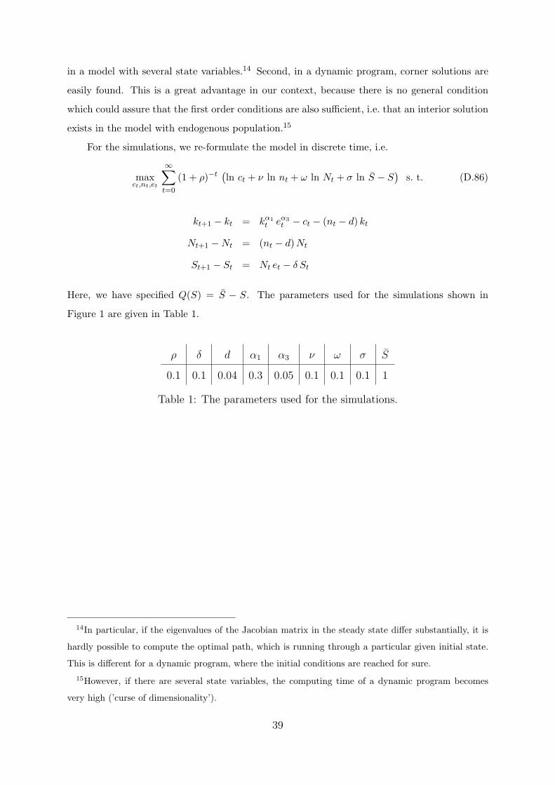
in a model with several state variables.14 Second, in a dynamic program, corner solutions are

easily found. This is a great advantage in our context, because there is no general condition

which could assure that the first order conditions are also sufficient, i.e. that an interior solution

exists in the model with endogenous population.15

For the simulations, we re-formulate the model in discrete time, i.e.

maxct,nt,et

∞∑t=0

(1 + ρ)−t(ln ct + ν ln nt + ω ln Nt + σ ln S − S

)s. t. (D.86)

kt+1 − kt = kα1t eα3

t − ct − (nt − d) kt

Nt+1 −Nt = (nt − d)Nt

St+1 − St = Nt et − δ St

Here, we have specified Q(S) = S − S. The parameters used for the simulations shown in

Figure 1 are given in Table 1.

ρ δ d α1 α3 ν ω σ S

0.1 0.1 0.04 0.3 0.05 0.1 0.1 0.1 1

Table 1: The parameters used for the simulations.

14In particular, if the eigenvalues of the Jacobian matrix in the steady state differ substantially, it is

hardly possible to compute the optimal path, which is running through a particular given initial state.

This is different for a dynamic program, where the initial conditions are reached for sure.

15However, if there are several state variables, the computing time of a dynamic program becomes

very high (’curse of dimensionality’).

39