environmental monitoring branch monitoring branch 1001 i street, ... excel. a more detailed ... crop...

Department of Pesticide Regulation Environmental Monitoring Branch

1001 I Street, P.O. Box 4015 Sacramento, California 95812

Study 263: Protocol to Model Pesticide Concentration and Mass Loading from Rice Paddy:

Theoretical Considerations and Model Evaluation

Yuzhou Luo January 2010 (corrected October 2010)

1. Introduction According to Crop Production 2008 Estimates by National Agricultural Statistics Service (USDA, 2008), California is the second largest U.S. rice-growing state with 519 thousand acres for rice production. About 90% of California rice is grown in the Sacramento Valley. Pesticides continue to be a critical and growing component of California rice technology. According to the Pesticide Use Report maintained by Department of Pesticide Regulation, statewide use of pesticides in rice fields was 1.9 million kg in 2008 (DPR, 2008). Pesticides regularly used in the Sacramento Valley for rice production include propanil, copper sulfate, and thiobencarb. Pesticide use has a potential to cause aquatic toxicity since flooded rice fields dominate the landscape of the Sacramento Valley and the agricultural drains in the rice-producing regions are tributaries of the Sacramento River. In late 1970s and early 1980s, fish kills have been reported in the Colusa Basin agricultural drains receiving rice culture discharge contaminated with thiocarbamate herbicides (SWRCB, 1990; Bennett et al., 1998). In 1983 an off taste in the municipal drinking water of the City of Sacramento was attributed to thiobencarb sulfoxide (Cornacchia et al., 1984). As a result, monitoring program of pesticides from rice discharge water was developed since 1980. In 1990, the Central Valley Regional Water Quality Control Board set performance goals for pesticides used in rice production, as target concentrations not to be exceeded in water both in the agricultural drains and in drinking water sources. To meet the performance goals, Department of Pesticide Regulation instituted a variety of measures, primarily the holding of pesticides on fields or closed water system for sufficient degradation before water release. The compliance with performance goals is mainly verified by monitoring data from sampling sites located on major streams and water treatment plant intakes. Submitted monitoring data are usually associated with low resolutions in both space and time, and thus insufficient to characterize the spatial distribution and the main sources of pesticide residues. Therefore, mathematic models are needed to characterize effects of pesticide use, management practices, and environmental factors on pesticide fate and distribution. In addition, the regulatory burden has evolved currently to consider negative impacts of pesticides on aquatic organisms. Detailed information for pesticide residues, such as the magnitude, timing and frequency of peak concentrations, are required to examine the ecosystem exposure by the use of pesticides in rice

paddies. While the monitoring data is usually not available for the required information, continuous modeling at field scale could provide reasonable estimates for a decision making process toward meeting regulatory requirements and improving management practices. Rice pesticide modeling can be utilized to analyze the mechanisms of pesticide fate and transport processes, and evaluate management practices in controlling pesticide discharge from paddy fields. Successful simulation of rice pesticide fate and transport is based on accurate mathematical description of pesticide behaviors in various components and construction of the relational model that would adequately represent the governing processes in the rice field condition. Therefore, mathematic models are required to handle flood-related pesticide simulations such as pesticide volatilization, partitioning, degradation, and discharge. Currently, a number of simulation models for pesticides used in paddy rice production are available (as reviewed later in this protocol); however, only a few of them have been applied in California rice fields. Rice production in California presents a unique adaptation of rice culture to California’s weather, land, and water conditions. Therefore, models developed and calibrated in other regions could not be directly applied to evaluate pesticide fate and transport in rice fields of California. In this study, popular models for rice pesticide simulation will be assessed theoretically and practically for their capability to simulate pesticide fate and distribution under California field conditions. The results of this study are anticipated to provide guidance for model selection and model improvement for use for registration purposes. 2. Objectives This study is mainly designed to evaluate the capability and limitations of existing models in simulating pesticide fate and transport in rice paddies. Specific objectives include: [1] to review previous studies and determine the importance of each individual transport and transformation processes of rice pesticides; [2] to evaluate available calibration datasets, and provide recommendations for future monitoring studies; [3] to compare the model equations and algorithms of selected models for rice pesticides, and apply them to the field conditions of California rice culture; and [4] to identify model capability and limitations in simulating pesticide fate and transport, and recommend model(s) for further investigation and development for pesticide registration purposes in California. 3. Personnel This study will be conducted by Environmental Scientist Yuzhou Luo under the supervision of Senior Environmental Scientist Sheryl Gill and the guidance of Research Scientists III: Bruce Johnson, Frank Spurlock, and John Troiano. Questions concerning this protocol should be directed to project leader Yuzhou Luo at (916) 445-2090 or by email at [email protected].

4. Study Plan 4.1 Model Selection Three rice models were selected for model evaluation (Table 1). PFAM (Pesticide in Flooded Agriculture Model) was developed by USEPA Office of Pesticides (USEPA, 2009). PFAM was designed specifically for use in a regulatory setting responding to the data available during a regulatory assessment. The model considered chemical transformation processes, i.e., hydrolysis, bacterial metabolism, photolysis, and sorption in two regions of littoral region and benthic region. Mathematic formulations are heavily borrowed from the USEPA EXAMS model (Burns, 2000). Changes of temperature, water levels, wind speed, etc and the resulting changes in degradation rates occur on a daily time step. A Windows-based GUI (graphic user interface) is also available. Table 1. Summary of selected models in this study Model Institute Notes PFAM (Young, 2009) USEPA R&D release,

FORTRAN program PCPF (Watanabe and Takagi, 2000a, 2000b)

Tokyo University of Agriculture and Technology

VBA Macro

RICEWQ (Williams et al., 2008)

Waterborne Environmental, Inc. FORTRAN program

PCPF (Pesticide Concentration in Paddy Field) is a lumped-parameter model that simulates the fate and transport of pesticides in the two compartments of paddy water and paddy soil at daily time step. In addition to irrigation, precipitation, overflow/controlled drainage, and evapotranspiration, the model also considers water loss by lateral seepage and vertical percolation. The model program was coded using Visual Basic for Application in Microsoft Excel. A more detailed model description is documented by Watanabe and Takagi (2000a; 2000b) RICEWQ (Rice Water Quality) was developed to evaluate the dissipation and runoff of agrochemicals from their use on aquatic crops. The latest version of RICEWQ (1.7.3) was released by Waterborne Environmental Inc. in 2008 (Williams et al., 2008). Major components of the model include water balance, pesticide application, crop growth, and water quality. Water quality algorithms were derived in part from the USDA SWRRBWQ model (Simulator for Water Resources in Rural Basins – Water Quality) (Arnold et al., 1991). A Windows-based GUI is available but not all functions are implemented in the model. 4.2 Data Collection Collection of data for model evaluation will continue through the entire project. Models will be applied to the 16 rice fields taken from 5 studies in Colusa and Glenn Counties (Table 2). Field conditions (such as rice paddy dimension, soil properties, and weather), management practices, and measured data are retrieved from digital or printed versions of the papers and reports. All data are reorganized into a uniform format, consistent with the general requirements of model data inputs. For example, dates for seeding and application are recorded by Julian days, while

water management and sampling are labeled in a relative way of “days after application” (DAA). Formatted datasets would significantly facilitate future model parameterization and subsequent evaluation processes. Detailed data for field characteristics and pesticide measurements were provided in the Appendix. Table 2. Summary of field experiments used for model comparison Reference Year Area, ha Pesticide

1983 37 thiobencarb Study 1 (Ross and Sava, 1986) 1983 41 molinate 1987 45 bentazon 1987 33 bentazon

Study 2 (Ross et al., 1989)

1987 58 bentazon 1988 24 carbofuran 1988 34 carbofuran

Study 3 (Nicosia et al., 1991a)

1988 32 carbofuran 1989 24 bensulfuron methyl 1989 16 bensulfuron methyl

Study 4 (Nicosia et al., 1991b)

1989 17 bensulfuron methyl 1991 15.1 methyl parathion 1991 34.4 methyl parathion 1991 41.8 methyl parathion 1991 36.4 methyl parathion

Study 5 (Kollman et al., 1992)

1991 28.3 methyl parathion 4.3 Model Evaluation Model evaluation and comparison will involve two phases: theoretical comparison based on model descriptions, assumptions, and equations taken from literatures and practical evaluation by comparing model predictions to monitoring data in selected field conditions (Table 2). In theoretical comparison, models will be compared by the following aspects: [1] Input parameters and methods for parameter estimation [2] Compartments, phases, processes, and mechanisms included in models [3] Numerical methods for dynamic mass balance [4] Adjustment of rate constants to environmental conditions (temperature, pH, radiation) [5] Flexibility for pesticide-specific properties, e.g., slow release, biphasic degradation [6] Flexibility for flood-related management, e.g., continuous flood, emergency release, weir

height control, irrigation rate control, pre-flood pesticide application [7] Availability of output variables An integrated model environment is proposed to facilitate model application with case studies. All models in this study will be incorporated into this interface and driven by a single standard input dataset. Input data of landscape characteristics, weather condition, rice management, and pesticide application are taken from the literature of field experiments (Table 2). GIS-based spatial analysis is utilized to support model parameterization. For example, if soil property or daily weather data are not available in the literature, the data could be automatically retrieved

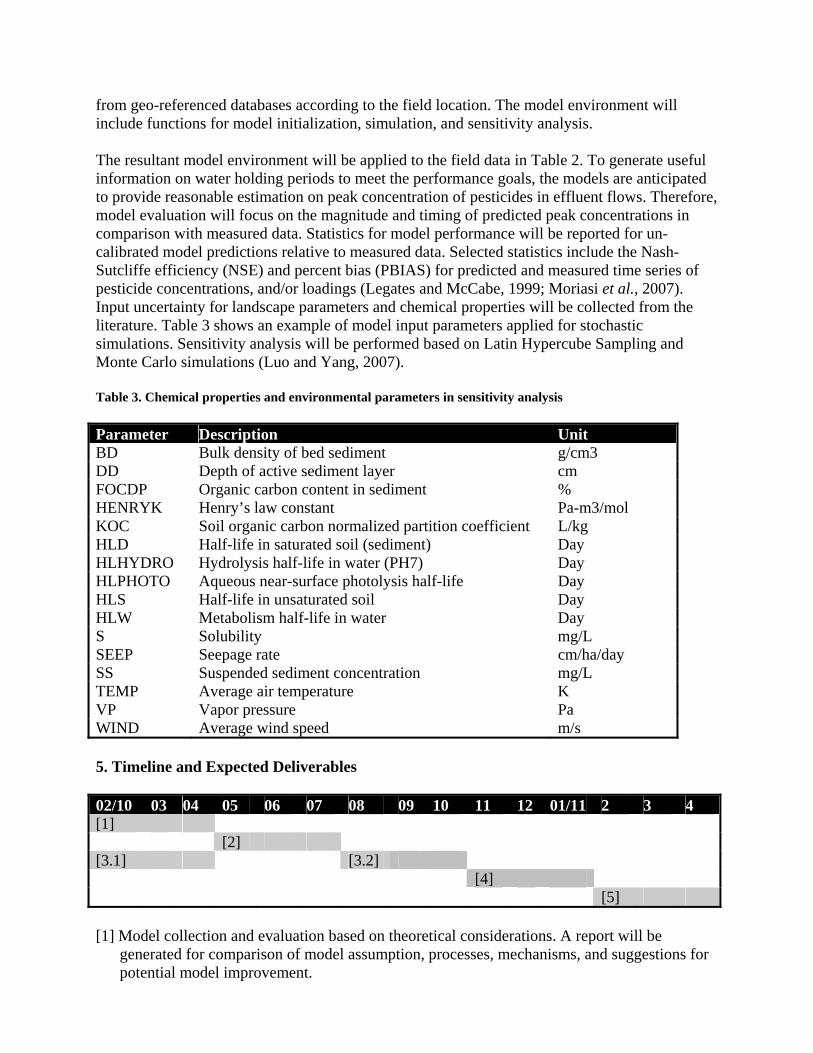
from geo-referenced databases according to the field location. The model environment will include functions for model initialization, simulation, and sensitivity analysis. The resultant model environment will be applied to the field data in Table 2. To generate useful information on water holding periods to meet the performance goals, the models are anticipated to provide reasonable estimation on peak concentration of pesticides in effluent flows. Therefore, model evaluation will focus on the magnitude and timing of predicted peak concentrations in comparison with measured data. Statistics for model performance will be reported for un-calibrated model predictions relative to measured data. Selected statistics include the Nash-Sutcliffe efficiency (NSE) and percent bias (PBIAS) for predicted and measured time series of pesticide concentrations, and/or loadings (Legates and McCabe, 1999; Moriasi et al., 2007). Input uncertainty for landscape parameters and chemical properties will be collected from the literature. Table 3 shows an example of model input parameters applied for stochastic simulations. Sensitivity analysis will be performed based on Latin Hypercube Sampling and Monte Carlo simulations (Luo and Yang, 2007). Table 3. Chemical properties and environmental parameters in sensitivity analysis Parameter Description Unit BD Bulk density of bed sediment g/cm3 DD Depth of active sediment layer cm FOCDP Organic carbon content in sediment % HENRYK Henry’s law constant Pa-m3/mol KOC Soil organic carbon normalized partition coefficient L/kg HLD Half-life in saturated soil (sediment) Day HLHYDRO Hydrolysis half-life in water (PH7) Day HLPHOTO Aqueous near-surface photolysis half-life Day HLS Half-life in unsaturated soil Day HLW Metabolism half-life in water Day S Solubility mg/L SEEP Seepage rate cm/ha/day SS Suspended sediment concentration mg/L TEMP Average air temperature K VP Vapor pressure Pa WIND Average wind speed m/s 5. Timeline and Expected Deliverables 02/10 03 04 05 06 07 08 09 10 11 12 01/11 2 3 4 [1] [2] [3.1] [3.2] [4] [5] [1] Model collection and evaluation based on theoretical considerations. A report will be

generated for comparison of model assumption, processes, mechanisms, and suggestions for potential model improvement.

[2] Interface development. A graphic user interface will be developed for rice pesticide models. [3] Model application to the field condition of California rice culture, with [3.1] data collection

and [3.2] model application to selected field scenarios. Report for model performance in case studies will be submitted.

[4] Sensitivity analysis to determine the key parameters and governing processes in rice pesticide fate and transport simulated by each model. Report for sensitivity analysis will be submitted.

[5] Final report preparation. References Arnold, J. G., J. R. Williams, R. H. Griggs and N. B. Sammons (1991). SWRRBWQ - A Basin

Model for Assessing Management Impacts on Water Quality. USDA. ARS, Grassland, Soil, and Water Research Laboratory, Temple, TX.

Bennett, K. P., N. Singhasemanon, N. Miller and R. Gallavan (1998). Rice pesticides monitoring in the Sacramento Valley, 1995, http://www.cdpr.ca.gov/docs/emon/pubs/ehapreps/eh983execs.pdf (accessed 01/2010). Department of Pesticide Regulation. Sacramento, CA.

Burns, L. A. (2000). Exposure analysis modeling system (EXAMS): user manual and system documentation (EPA/600/R-00/81-023). U.S. Environmental Protection Agency. Washington, DC.

Cornacchia, J. W., D. B. Cohen, G. W. Bowes, R. J. Schnagl and M. B.L. (1984). Rice herbicides: molinate and thiobencarb. CSWRCB Special Project Report 84-4sp. State Water Resources Control Board. Sacramento, CA.

DPR (2008). The top 100 sites in total statewide pesticide use in 2008. http://www.cdpr.ca.gov/docs/pur/pur08rep/top100_sites.pdf (accessed 01/2010). Department of Pesticide Regulation. Sacramento, CA.

Kollman, W. S., P. L. Wofford and J. White (1992). Dissipation of methyl parathion from flooded commercial rice fields, EH 92-03. California Environmental Protection Agency, Department of Pesticide Regulation.

Legates, D. R. and G. J. McCabe (1999). Evaluating the use of “Goodness-of-Fit” measures in hydrologic and hydroclimatic model and validation. Water Resources Research, 35(1): 233-241.

Luo, Y. and X. Yang (2007). A multimedia environmental model of chemical distribution: fate, transport, and uncertainty analysis. Chemosphere, 66(8): 1396-1407.

Moriasi, D. N., J. G. Arnold, M. W. V. Liew, R. L. Bingner, R. D. Harmel and T. L. Veith (2007). Model evaluation guidelines for systematic quantification of accuracy in watershed simulations. Transaction of the American Society of Agricultural and Biological Engineers (ASABE), 50: 885-900.

Nicosia, S., N. Carr, D. A. Gonzales and M. K. Orr (1991a). Off-fields movement and dissipation of soil-incorporated carbofuran from three commercial rice fields. Journal of Environmental Quality, 20: 532-539.

Nicosia, S., C. Collison and P. Lee (1991b). Bensulfuron methyl dissipation in California rice fields, and residue levels in agricultural drains and the Sacramento River. Bulletin of Environmental Contamination and Toxicology, 47: 131-137.

Ross, L. J., S. Powell, J. E. Fleck and B. Buechler (1989). Dissipation of bentazon in flooded rice fields. Journal of Environmental Quality, 18: 105-109.

Ross, L. J. and R. J. Sava (1986). Fate of thiobencarb and molinate in rice fields. Journal of Environmental Quality, 15: 220-225.

SWRCB (1990). Sacramento River Toxic Chemical Risk Assessment, Publication 90-11WQ, State Water Resources Control Board, Sacramento, CA.

USDA (2008). California farm news: California crop production report 2008. United States Department of Agriculture, National Agricultural Statistics Service. Sacramento, CA.

USEPA (2009). A flooded agriculture model for pesticide risk assessments: model development (Draft). U.S. Environmental Protection Agency, Office of Pesticides, Washington, DC.

Watanabe, H. and K. Takagi (2000a). A simulation model for predicting pesticide concentrations in paddy water and surface soil. I. Model development. Environmental Technology, 21: 1379–1391.

Watanabe, H. and K. Takagi (2000b). A simulation model for predicting pesticide concentrations in paddy water and surface soil. II. Model validation and application. Environmental Technology, 21: 1393–1404

Williams, W. M., A. M. Ritter, C. E. Zdinak and J. M. Cheplick (2008). RICEWQ: Pesticide Runoff Model For Rice Crops, Users Manual And Program Documentation, Version 1.7.3. Waterborne Environmental, Inc., Leesburg, VA.

Young, D. F. (2009). A Flooded Agriculture Model for Pesticide Risk Assessments: Model Development (Draft). Environmental Fate and Effects Division, Office of Pesticides, U.S. Environmental Protection Agency, Washington, SC.

Appendix. Field Characteristics and Measured Data Data from Kollman et al. (1992) Summary: Five fields in Colusa county and Glenn county with methyl parathion application in 1991 Field ID

Size (ha)

Soil Seeding, Date (Julian)

Application, Date (Julian)

Management, Date (DAA), depth (mm)

1 15.1 Wekoda silty clay OC=1%

4/21 (111) 5/1 (121) Depth=8.8-19.2 (14.7)

2 34.4 Wekoda silty clay OC=.5%

5/1 (121) 5/11 (131) 5/27 (16) drain Depth=4.3-9.0 (6.85)


5/5 (125) 5/17 (137) 6/2 (16) drain 6/6 (20) flood Depth=3.9-13.8 (10.7)


5/5 (125) 5/17 (137) 6/2 (16) drain 6/6 (20) flood Depth=3.3-11.8 (8.5)

5 28.3 Sunnyvale clay OC=1%

5/14 (134) 5/28 (148) Soil incorporation 5/31 (3) flood to 9.5 6/1 (4) flood to 14.1 Depth=5.3-14.1 (9.3)

Notes: Wekoda silty clay (Aquic Chromoxererts), 4% sand/ 51% silt/ 45% clay Sunnyvale clay (Typic Calciaquoll), 14% sand/ 40% silt/ 47% clay Application rate = 0.7 kg/ha for all fields DAA=”days after application” Table 4. Measurements, Field 1

Concentration (µg/L) DAA Water depth (cm) Mean ±Range

Mass (kg/ha)

2* 19.2 121.3 29.444 .2329 3 18.8 70.88 6.307 .13297 4 18.4 43.58 10.875 .08001 5 17.3 37.51 5.056 .06475 7 16.9 14.12 2.390 .02381 9 13.5 6.09 0.141 .0082 11 13.1 3.25 0.191 .00425 15 10.1 1.89 0.728 .0019 19 8.8 0.54 0.035 .00047 23 11.3 0.3 0.078 .00034 * Measurements for field 1 at 2 DAA are questionable and not used in the statistical analysis (Kollman et al., 1992).

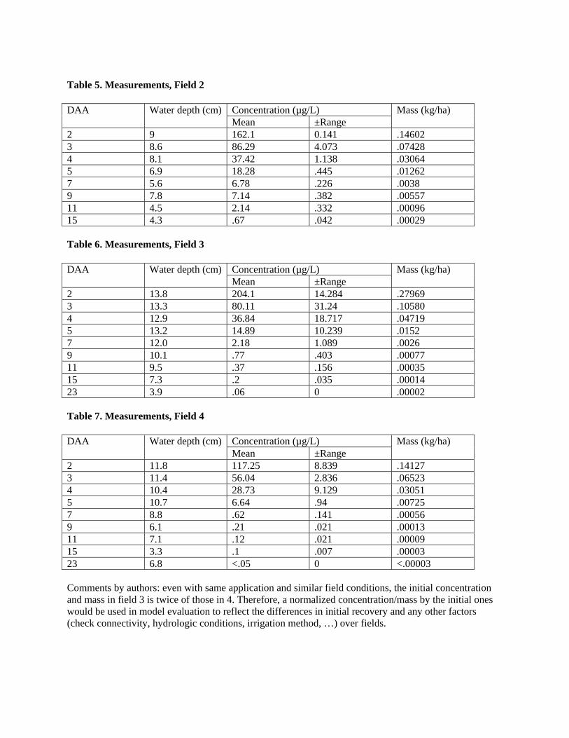
Table 5. Measurements, Field 2


Mass (kg/ha)

2 9 162.1 0.141 .14602 3 8.6 86.29 4.073 .07428 4 8.1 37.42 1.138 .03064 5 6.9 18.28 .445 .01262 7 5.6 6.78 .226 .0038 9 7.8 7.14 .382 .00557 11 4.5 2.14 .332 .00096 15 4.3 .67 .042 .00029 Table 6. Measurements, Field 3


Mass (kg/ha)

2 13.8 204.1 14.284 .27969 3 13.3 80.11 31.24 .10580 4 12.9 36.84 18.717 .04719 5 13.2 14.89 10.239 .0152 7 12.0 2.18 1.089 .0026 9 10.1 .77 .403 .00077 11 9.5 .37 .156 .00035 15 7.3 .2 .035 .00014 23 3.9 .06 0 .00002 Table 7. Measurements, Field 4


Mass (kg/ha)

2 11.8 117.25 8.839 .14127 3 11.4 56.04 2.836 .06523 4 10.4 28.73 9.129 .03051 5 10.7 6.64 .94 .00725 7 8.8 .62 .141 .00056 9 6.1 .21 .021 .00013 11 7.1 .12 .021 .00009 15 3.3 .1 .007 .00003 23 6.8 <.05 0 <.00003 Comments by authors: even with same application and similar field conditions, the initial concentration and mass in field 3 is twice of those in 4. Therefore, a normalized concentration/mass by the initial ones would be used in model evaluation to reflect the differences in initial recovery and any other factors (check connectivity, hydrologic conditions, irrigation method, …) over fields.

Table 8. Measurements, Field 5


Mass (kg/ha)

3 9.5 66.43 8.04 .06354 4 14.1 44.53 11.738 .06321 5 12.6 21.73 2.213 .02757 7 11.1 4.04 .396 .00451 9 5.3 1.07 .424 .00057 11 8.2 .84 .226 .00069 15 7.3 .2 0 .00015 19 9.1 .25 .1354 .00023 23 6.8 <.05 0 <.00003 Data from Nicosia et al. (1990) Summary: Three fields in Colusa county and Glenn county with soil-incorporated carbofuran application in 1988 Table 9. Field conditions Field ID

Size (ha)




1 24 [a] OC=2.4%

4/27 (118) 4/16 (107) 1.10 kg/ha 1.10 kg/ha

4/26 (10), flood Depth=11

2 34 [a] OC=2.2%

4/18 (109) 4/12 (103) 1.21 kg/ha 1.81 kg/ha

4/18 (6), flood 5/27 (45), drain 5/28 (46), flood Depth=15.1

3 32 [b] OC=2.8%

4/20 (111) 4/14 (105) .64 kg/ha .66 kg/ha

4/18 (4), flood 5/31 (47), drain 6/1 (48), flood Depth=18.3

[a] mix of Hiilgate clay (Typic Pelloxerert), and Myers clay (Entic Chromoxerert) [b] Willows clay (Typic Pelloxerert) First application rates are for the whole field, latter ones for the bottom paddy only Background concentration in soil = 0.02mg/kg

Table 10. Measurements, Field 1 (water depth = 11 cm)


Mass (kg/ha)

10 4.239385 0.00466323 4.730442 0.00520336 15.95714 0.01755337 12.81358 0.01409538 11.44168 0.01258639 14.09263 0.01550242 6.245313 0.0068743 2.806244 0.00308744 2.168743 0.00238645 3.893758 0.00428346 2.623974 0.00288647 2.600059 0.0028649 2.89999 0.0031950 1.603442 0.00176451 0.482293 0.00053152 0.500001 0.0005553 0.477207 0.00052554 0.787499 0.00086655 0.400001 0.0004456 0.4 0.0004457 0.426041 0.00046958 0.863541 0.0009559 0.437499 0.00048160 0.85476 0.0009461 1.746881 0.00192262 2.533337 0.00278763 5.251031 0.00577664 4.100059 0.0045165 4.523196 0.00497666 4.537515 0.00499167 2.007293 0.00220868 2.027087 0.0022369 1.075001 0.00118370 0.692709 0.00076271 0.633333 0.00069772 1 0.001173 0.983332 0.00108274 0.600001 0.0006675 0.600001 0.0006676 0.599999 0.0006677 0.594793 0.00065478 0.500001 0.0005579 0.499999 0.0005580 0.500001 0.0005581 0.791668 0.00087182 1.000001 0.0011

Table 11. Measurements, Field 2 (water depth = 15.1 cm)


Mass (kg/ha)

6 12.02663 0.018167 7.327463 0.0110648 7.927084 0.011979 6.665624 0.010065

10 7.510417 0.01134111 6.575002 0.00992812 5.287499 0.00798413 4.215626 0.00636614 4.205627 0.0063515 4.782303 0.00722116 5.700025 0.00860729 15.65524 0.02363930 21.57431 0.03257731 28.03334 0.0423332 26.95626 0.04070433 15.23125 0.02299936 6.053998 0.00914237 4.601051 0.00694838 2.416669 0.00364939 3.021875 0.00456340 2.487499 0.00375641 2.128124 0.00321342 1.587499 0.00239743 1.440624 0.00217544 1.200003 0.00181245 1.199988 0.00181248 4.259987 0.00643349 1.313542 0.00198350 1.35 0.00203951 1.022916 0.00154552 1.237502 0.00186953 1.585419 0.00239454 1.393751 0.00210555 1.253128 0.00189256 0.78125 0.0011857 0.616666 0.00093158 0.999998 0.0015159 0.593748 0.00089760 0.400002 0.00060461 0.400002 0.00060462 0.399999 0.00060463 0.399997 0.00060464 0.578129 0.00087365 0.699999 0.00105766 0.7 0.001057

Table 12. Continued- Measurements, Field 2 (water depth = 15.1 cm)


Mass (kg/ha)

67 1.166676 0.00176268 1.499999 0.00226569 1.5 0.00226570 1.458331 0.00220271 0.999996 0.0015172 0.999996 0.0015173 1 0.0015174 1.220831 0.00184375 1.399999 0.00211476 1.400002 0.00211477 1.404163 0.0021278 1.599999 0.00241679 1.599997 0.00241680 1.600003 0.00241681 1.600001 0.00241682 1.558334 0.00235383 0.600001 0.00090684 0.600002 0.00090685 0.600002 0.00090686 0.600002 0.000906

Table 13. Measurements, Field 3 (water depth = 18.3 cm)


Mass (kg/ha)

5 22.80773 0.0417386 16.675 0.0305157 10.21055 0.0186858 15.10625 0.0276449 14.3 0.026169

10 7.913542 0.01448211 9.273964 0.01697112 7.611465 0.01392913 5.506248 0.01007614 6.351049 0.01162215 7.000014 0.0128134 7.300003 0.01335935 5.766667 0.01055336 6.110352 0.01118237 6.777606 0.01240338 7.056984 0.01291439 5.050705 0.00924340 5.831347 0.01067141 4.265627 0.00780642 3.38767 0.00619943 2.616666 0.00478844 2.42412 0.00443645 1.20893 0.00221246 2.226978 0.00407547 2.900002 0.00530750 3.300012 0.00603951 2.138663 0.00391452 1.098958 0.00201153 0.986079 0.00180554 0.8 0.00146455 0.875 0.00160156 1.54375 0.00282557 0.718751 0.00131558 1 0.00183

Data from Nicosia et al. (1991) Summary: Three fields in Colusa county and Glenn county with Bensulfuron Methyl (BSM) application in 1989 Table 14. Field conditions Field ID

Size (ha)




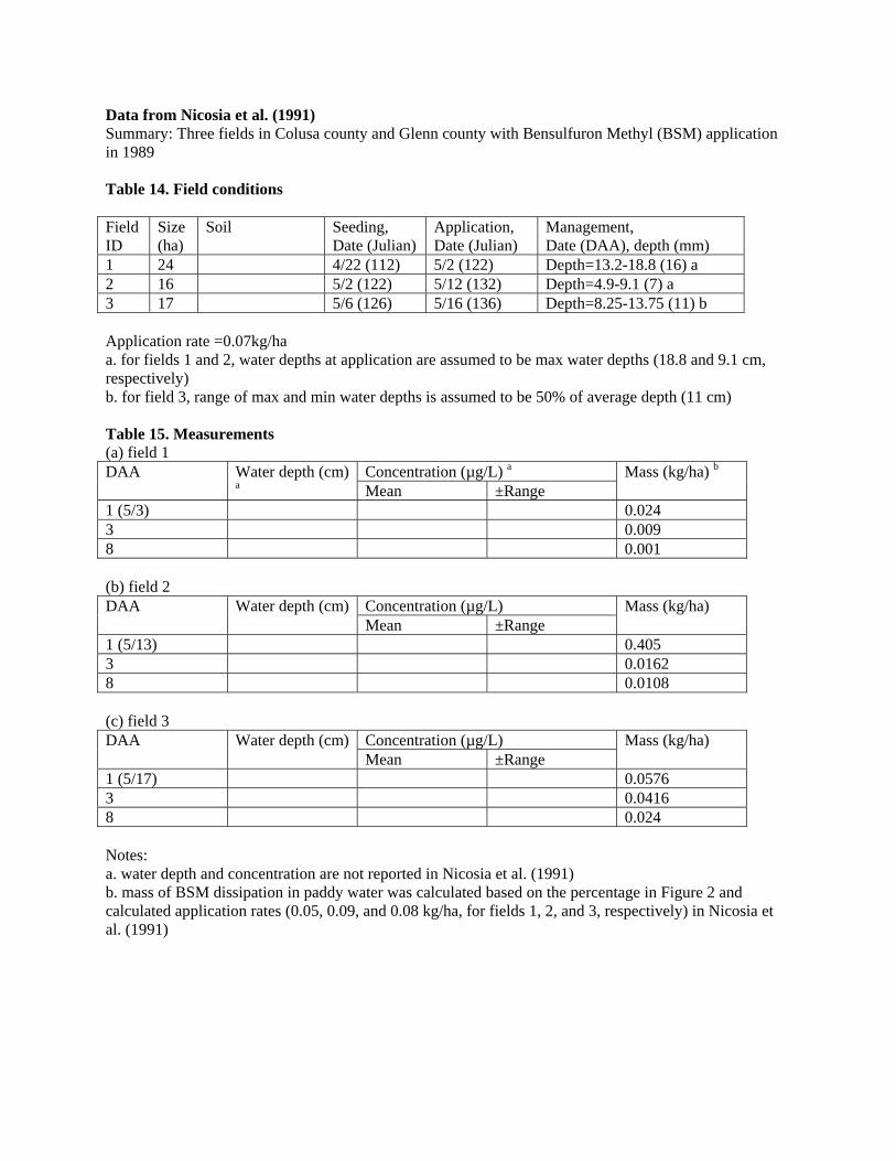
1 24 4/22 (112) 5/2 (122) Depth=13.2-18.8 (16) a 2 16 5/2 (122) 5/12 (132) Depth=4.9-9.1 (7) a 3 17 5/6 (126) 5/16 (136) Depth=8.25-13.75 (11) b Application rate =0.07kg/ha a. for fields 1 and 2, water depths at application are assumed to be max water depths (18.8 and 9.1 cm, respectively) b. for field 3, range of max and min water depths is assumed to be 50% of average depth (11 cm) Table 15. Measurements (a) field 1

Concentration (µg/L) a DAA Water depth (cm) a Mean ±Range

Mass (kg/ha) b

1 (5/3) 0.024 3 0.009 8 0.001 (b) field 2


Mass (kg/ha)

1 (5/13) 0.405 3 0.0162 8 0.0108 (c) field 3


Mass (kg/ha)

1 (5/17) 0.0576 3 0.0416 8 0.024 Notes: a. water depth and concentration are not reported in Nicosia et al. (1991) b. mass of BSM dissipation in paddy water was calculated based on the percentage in Figure 2 and calculated application rates (0.05, 0.09, and 0.08 kg/ha, for fields 1, 2, and 3, respectively) in Nicosia et al. (1991)

Data from Ross and Sava (1986) Summary: Two fields in Glenn county with thiobencarb and molinate applications in 1983 Table 16. Field conditions Field ID

Size (ha)

Soil a Seeding, Date (Julian)



1 37 [a] OC=?%

5/21 (141) 5/30 (150) 4.48 kg/ha

Depth=21-31 (26) 6/7 (8),drained to 11-23 (17)

2 41 [a] OC=?%

5/27 (147) 6/1 (152) 4.48 kg/ha 6/6 (157) 3.14 kg/ha

Depth=12-24 (18) 6/21 (15) b, drained completely 6/24 (18) b, flood to 4-16 (10)

a. mix of Myers clay loam (Entic Chromoxerert) b. Days after second application

Table 17. Measurements, Field 1 (a) water data


Mass (kg/ha)

0 (5/30) 79 43 0.23 2 567 222 1.543 4 576 181 1.482 6 515 130 1.218 8 367 120 0.766 16 56 35 0.074 32 8 5 0.013 (b) other data DAA Concentration,

air (µg/m3) Evaporative flux (ng/cm2/h)

Concentration, soil (µg/kg)

Concentration, vegetation (µg/kg)

0 (5/30) 1.4 (0.7) 37 (34) 3250 (2000) 78 (275) 1 0.9 (0.4) 8 (6) 2 0.8 (0.3) 16 (9) 2880 (2490) 691 (429) 3 0.4 (0.1) 6 (4) 4 3350 (3030) 1750 (2200) 6 3860 (2890) 1360 (1250) 8 2020 (1180) 1280 (1080) 16 2260 (1180) 796 (902) 32 2330 (2770) 169 (138) DAA Mass, air (kg/ha) Mass, Soil

(kg/ha) Mass, vegetation (kg/ha)

0 (5/30) 0.028 1.578 3.33e-4 1 0.01 2 0.019 1.435 5.80e-4 3 0.007 4 1.668 1.57e-4 6 1.920 1.41e-4 8 1.007 1.98e-4 16 1.125 1.84e-4 32 1.159 1.60e-4

Table 18. Measurements, Field 2 (a) water data

Concentration (µg/L) DAA a Water depth (cm) Mean ±Range

Mass (kg/ha)

-1 1880 767 0 (6/6) 3430 420 6.136 2 2450 1500 4.150 4 1760 1300 2.946 8 646 239 0.771 16 32 13 42 0.012 a. days after the second application (b) other data DAA Concentration,

air (µg/m3) Evaporative flux (ng/cm2/h)

Concentration, soil (µg/kg)

Concentration, vegetation (µg/kg)

-1 1410 (657) 498 (213) 0 (6/6) 37 (34) 575 (64) 1450 (1210) 918 (580) 1 8 (6) 193 (55) 2 16 (9) 110 (83) 1560 (875) 423 (309) 3 6 (4) 58 (36) 4 1680 (1150) 380 (325) 8 2210 (1330) 177 (177) 16 1330 (1430) 295 (203) 32 656 (582) 21 (33) DAA Mass, air (kg/ha) Mass, Soil

(kg/ha) Mass, vegetation (kg/ha)

-1 0 (6/6) 0.665 0.732 1.20 e-4 1 0.224 2 0.127 0.792 2.84 e-4 3 0.050 4 0.853 1.98 e-4 8 1.120 2.64 e-4 16 0.711 6.60 e-4 32 0.332 2.59 e-4

Data from Ross et al. (1989) Summary: Two fields in Yuba, Glenn, and Butte counties with bentazon application in 1987 Table 19. Field conditions Field ID

Size (ha)



Management, Date (DAA), depth (mm) a

1 45 Canejo loam (Pachic Haploxerolls) OC=?%

4/19 (109) 5/27 (147) 1.12 kg/ha

Drained before application 5/31 (4) ~6/3 (7). flood Depth=2.25~3.75 (3)

2 33 Myers clay loam (Entic Chromoxerets) OC=?%

4/20 (110) 5/28 (148) 1.12 kg/ha


3 58 Clay OC=?%

4/30 (120) 6/12 (163) 1.12 kg/ha


a. range of max and min water depths is assumed to be 50% of average depth

Table 20. Measurements (a) Field 1


Mass (kg/ha)

0 0.370165 1524.359 513.1601 0.0471831 0.183747 1799.441 115.4701 0.0255632 3.616379 365.8548 500.8326 0.0613973 4.608909 196.7887 470.8857 0.045234 3.711744 79.1791 116.6726 0.0211215 5.638587 55.10526 45.07771 0.0228516 4.723197 113.5 109.0245 0.0477427 5.053031 111.0256 76.86352 0.0515488 8.142683 121.7333 81.85353 0.07246

10 7.024651 50.40994 49.16045 0.03220612 10.98648 50.05492 59.11404 0.04846616 12.88282 25.17401 20.6207 0.02767132 13.13626 17.16667 12.37437 0.020981

har 18.26363 ND ND ND (b) Field 2


Mass (kg/ha)

0 0.3729 1327.059 152.7525 0.046421 0.317776 1411.765 212.132 0.0309682 3.573367 196.1111 626.2683 0.0319593 5.415114 298.9182 373.1398 0.0843744 6.513019 242.1007 263.5077 0.1484495 10.85866 159.3103 169.2139 0.1520996 15.16991 75.94972 96.20203 0.1118937 15.36378 103.5 143.0682 0.1533338 14.92485 92.88889 129.2685 0.137613

10 15.18999 62.83152 93.97368 0.09515212 16.75241 65.67568 111.4038 0.1116 17.85667 65.07442 81.38968 0.11515232 15.72146 26.55236 37.89487 0.041741

har 22.4149 1.409 1.732412 ND

(c) Field 3


Mass (kg/ha)

0 NA NA NA NA 1 NA NA NA NA 2 4.746343 296.0494 301.7173 0.1268783 8.869315 131.7452 171.6081 0.1094394 11.10674 50.77438 63.99573 0.0545355 9.493943 54.48315 45.74203 0.0513126 10.83437 42.39602 25.71874 0.0450887 11.83386 68.27761 40.05625 0.0726138 11.03753 24.67539 13.45561 0.024937

10 10.04432 47.5918 39.03498 0.04608112 8.993049 32.4994 25.33009 0.02871616 8.526221 21.85229 14.80721 0.0176932 21.8035 2.405542 1.167619 0.005053

har 9.826974 0.694828 0.377492 ND Average water depth, concentration, and mass are based on the average values at the three measured paddies in each field. If only two paddies are measured in a specific day, average will be based on those two measurements. If less than two paddies are measured, NA is provided.

environmental monitoring branch monitoring branch 1001 i street, ... excel. a more detailed ... crop...

Documents