environmental measurement

John D. Garrison, et. al.. "Environmental Measurement."

Copyright 2000 CRC Press LLC. <http://www.engnetbase.com>.

EnvironmentalMeasurement

73.1 Meteorological MeasurementMeasurement of the Atmospheric Variables • United States Weather Service Facilities

73.2 Air Pollution MeasurementSpectroscopic Principles • Particulate Sampling • Slow Ambient Monitoring • Fast Ambient Monitoring • Remote Monitoring • Emissions Monitoring

73.3 Water Quality MeasurementTheory • Instrumentation and Applications

73.4 Satellite Imaging and SensingWhat Can Be Seen from Satellite Imagery • Management and Interpretation of Satellite Data • The Future in Satellite Imaging and Sensing

73.1 Meteorological Measurement

John D. Garrison and Stephen B. W. Roeder

Meteorological measurements are measurements of the physical properties of the atmosphere. Thesemeasurements are made at all elevations in the troposphere and the stratosphere. For measurementsmade at elevations above ground or tower level, instruments can be carried aloft by balloons, rockets,or airplanes. Ground radar is used to detect the presence of water in the form of droplets or ice crystalsat all elevations and the winds associated with them. Lidar (optical radar) of selected wavelengths is usedto detect the presence and amount of aerosols and other constituents of the atmosphere and to determinecloud height. Instruments on satellites measure properties of the atmosphere at all elevations.

Quantities measured are: temperature, pressure, humidity, wind speed, wind direction, visibility, thepresence and amount of precipitation, cloud amount, cloud opacity, cloud type, cloud height, broadbandsolar (or shortwave) radiation, longwave radiation, ultraviolet radiation, and net radiation, sunshineduration, turbidity, and the amounts of trace gases such as NO, NO2, SO2, and O3. Some of the methodsand instruments used to measure a number of these variables are discussed in this handbook in sectionson pressure, temperature, humidity and moisture content, and air pollution monitoring. Additionalinformation of interest is in sections on resistive sensors, inductive sensors, capacitive sensors, satellitenavigation and radiolocation, and the sections under signal processing.

Meteorological measurements are made at individual sites, at several or many sites forming a localnetwork, or at much larger networks. Much of the emphasis now is on global networks covering theentire northern and southern hemispheres. Individuals and groups can make measurements for theirown purposes or they can use data provided by the various weather services. Weather service data are

John D. GarrisonSan Diego State University

Stephen B. W. RoederSan Diego State University

Michael BennettWillison Associates

Kathleen M. LeonardThe University of Alabama in Huntsville

Jacqueline Le MoigneNASA/GSFC - Code 935

Robert F. CrompNASA/GSFC - Code 930

© 1999 by CRC Press LLC

stored in archives that can cover many years of measurements. The U.S. National Climatic Data Center,Asheville, NC, has archived data produced from measurements at U.S. weather stations and other NationalOceanic and Atmospheric Administration (NOAA) measurement sources, including satellites. It also hasnon-U.S. data. These data can be purchased. The Web site where information concerning NOAA datacan be obtained is: <http://www.ncdc.noaa.gov/>. The U.S. National Renewable Energy Laboratory hasinformation on solar radiation and wind at Web site: <http://www.rredc.nrel.gov />. Data at Web sitescan often be retrieved by anonymous File Transfer Protocol (FTP).

Fabrication of meteorological instruments is usually done by companies specializing in these instru-ments. It is generally not economically feasible for individuals to fabricate their own instruments, unlesstheir particular application cannot use commercially available instruments. The problem usually reducesto the determination of which commercial instruments to purchase. This determination depends on cost,durability, accuracy, maintenance requirements, ease of use and the form of the output signal. A numberof instrument manufacturers and distributors market complete weather stations.

The instruments used for meteorological measurements are fabricated for use in the special environmentof the atmosphere. This environment varies with the latitude and longitude of the site and the elevationabove the ground and above sea level. A common requirement is that the instruments be protected fromadverse conditions that can cause errors in the measurement of the meteorological variables. For properoperation, some instruments (e.g., spectroradiometers) need to be in a temperature-controlled environ-ment. The sun’s heating can cause errors. Solar radiation can cause weathering of the instruments andshorten their useful life. Moisture from precipitation or dew can affect measurements adversely and alsocause weathering and corrosion of the instruments. Blowing dust or sand can cause weathering of theinstruments and affect the operation of mechanical parts. Insects, birds, and ice can also affect instrumentsadversely. Some gaseous constituents of the atmosphere can be corrosive. Packaging of the sensors andhousing of the instruments in enclosures can protect them, but this protection must not interfere withthe measurement of the meteorological variable. Packaging a sensor and putting the sensor in protectivehousing generally increases the response time of the sensor to changes in the meteorological variable it ismeasuring. Solar heating can be reduced by covering the sensor, its protective packaging, or housing witha white coating. Generally, housing or enclosures used to protect the instruments should be well ventilated.Sometimes a fan is used to draw air through the housing or enclosure to reduce solar heating and makethe air more representative of the outside air. Loss of measurement caused by loss of electric power canbe avoided by having backup power from batteries or motor-generators.

Another common requirement of meteorological measuring instruments is that they be calibrated beforeinstallation in the field. This is usually done by the manufacturer. For some applications, it may be importantthat the calibrations are traceable to NIST (National Institute of Standards and Technology) standards. Thecalibration should be checked routinely. Some instruments are constructed to be self-calibrating.

Generally, there is no reason to measure many of the meteorological variables to high precision. Thetemperature, humidity, and wind, for example, can vary in relatively short distances and sometimes inrelatively short times by amounts that are large compared to the accuracy of the measuring instruments.This is especially true near ground level. The exact value of a meteorological variable at a particular sitehas little meaning unless the density of measuring sites is very high. A mesoscale network with highdensity of measuring sites over a relatively small area might be of interest for ecological studies. Larger-scale or global networks have widely separated sites. For these networks it is important to install all ofthe instruments in a standard manner so as to reduce the effect of local fluctuations on the variation ofthe meteorological variables from site to site. Usually, this is done by placing them on a level, open areaaway from surrounding buildings and other obstructions and at a fixed distance above the ground. Theground should be drained ground and not easily heated to high temperature by the sun. In comparingtemperatures, one must be aware of the “heat island effect” of large cities; furthermore, an increase inthe degree of urbanization of a given site over time may affect the interpretation of the temperaturetrends observed.

The current trend is toward automatic measurement of meteorological variables at unattended siteswith automatic data retrieval and computer processing and analysis of the data. Large-scale networks


consisting of many stations covering a large area (e.g., the Northern Hemisphere) are used for regional,national, and global weather forecasting.

Measurement of the Atmospheric Variables

Temperature

The mean temperature of the atmosphere for each hour of the day at a particular site has a fairly regularannual and a diurnal variation when this mean temperature is an average over many years for each hourand day of the year. The temperature at a given site and time is a superposition of the mean temperatureand the fluctuations from this mean temperature caused by current cloud and wind conditions, the pasthistory of the air mass passing over the site, and interannual variations that are not yet well understood.

More detailed sources of information on temperature measurement include the earlier section in thishandbook on temperature measurement and References 1 through 5. The common methods of measuringatmospheric temperature include the following:

Electric Resistance Thermometer (RTD).The variation of the resistance of a metal with temperature is used to cause a variation in the currentpassing through the resistance or the voltage across it. The electric circuit used for the measurement oftemperature can utilize a constant current source, and temperature is determined from the voltage acrossthe resistance after the circuit is calibrated. Alternatively, a constant voltage source can be used with thecurrent through the resistance determining the temperature. Once the instrument is calibrated, it isgenerally expected to keep its calibration as long as electric power is supplied to the instrument. Com-monly, platinum RTD thermometers are made of a fixed length of fine platinum wire or a thin platinumfilm on an insulating substrate. The variation of the resistance as a function of temperature is approxi-mately linear over the range of temperature found in meteorological measurements. The quadraticcorrection term is quite small. The accuracy and reproducibility of the measurements and the ease ofusing an electric signal for transmission of data from remote unmanned sites makes electric resistancethermometers desirable for meteorological applications. Platinum is the best metal to use. With carefulcalibration and good circuit design, platinum resistance thermometers can measure temperature to asmall fraction of a degree, much better than the accuracy needed for meteorological measurements.

Thermistors.Thermistors usually consist of an inexpensive mixture of oxides of the transition metals. The log of theirresistance varies inversely with temperature. The change in resistance with temperature can be 103 to 106

times that of a platinum resistance thermometer. Their change in resistance with temperature is used todetermine temperature in the same manner as metal resistance thermometers. They are somewhat lowerin cost and are somewhat less stable than platinum resistance thermometers.

Bimetallic Strip.Bimetallic strips are discussed elsewhere in an earlier section. They are usually used for casual monitoringof inside and outside temperatures at dwellings and office buildings and for heating and cooling controls.The accuracy is generally about ±1°C. They are low in cost.

Liquid in Glass Thermometer.These are a well-known method of measuring temperature. They are usually used for casual monitoringof inside and outside temperatures at dwellings or office buildings. These thermometers are more difficultto read than meter or dial readings of temperature, do not lend themselves to electric transmission oftheir readings, and are easily broken. Their cost can be low.

Pressure

One standard atmosphere of pressure corresponds to 1.01325 ´ 105 pascals (N m–2) (14.6960 pounds persquare inch, 1.01325 bars, 1013.25 mbars, 760.00 mm Hg, or 29.920 in. Hg). This is approximately themean atmospheric pressure at sea level. Atmospheric pressure at sea level usually does not deviate more


than ±5% from one standard atmosphere. Atmospheric pressure decreases with altitude. Altitude mea-surements in airplanes are based on air pressure measuring instruments called altimeters. At about 5500 m(18,000 ft), the atmospheric pressure is half its sea level value. The following instruments are used tomeasure atmospheric pressure.

Mercury ManometerOriginally, barometric pressure was measured with a mercury manometer. This is a tube, about 1 m inlength, filled with mercury and inverted into an open dish of mercury. The height of the column ofmercury that the external pressure maintains in the tube is a measure of the external air pressure. Hence,one standard atmosphere is 760 mm Hg. While accurate, this device is awkward and has been replacedfor general use.

Aneroid Barometer.It consists of a partially evacuated chamber that can expand or contract in response to changing externalpressure. The evacuated chamber is often a series of bellows, so that the expansion and contraction occursin one dimension. Basic aneroid barometers, which are still in use, have a mechanical linkage to a pointergiving a reading on a dial calibrated to read air pressure. High-quality mechanical barometers can achievean accuracy of 0.1% of full scale. Aneroid barometers can also give electronic readout and eliminate themechanical linkage; this is more the standard for serious meteorological measurements. In one method,a magnet attached to the free end of the bellows is in proximity to a Hall effect probe. The Hall probeoutput is proportional to the distance between the magnet and the Hall probe.

Barometric pressure is also measured with an aneroid type of device that consists of a rigid cylindricalchamber with a flexible diaphragm at its end. A capacitor is created by mounting one fixed plate closeto the diaphragm and a second plate mounted on the diaphragm. As the diaphragm expands or contracts,the capacitance changes. Calibration determines the pressure associated with each value of capacitance.A range of 800 to 1060 millibars with an accuracy of ±0.3 millibars for ground-based measurements istypical. Setra Corporation produces this type of instrument for the U.S. National Weather Service ASOSnetwork, the latter produced by AAI Systems Management Incorporated. The ASOS network is discussedbelow. Measurement of pressure is also discussed elsewhere in this handbook.

Humidity

Instruments that determine the density or pressure of water in vapor form in the atmosphere, generallyeither measure relative humidity or they measure dewpoint temperature. The pressure of water vaporjust above a liquid water surface when the vapor is in equilibrium with the liquid water is the saturatedvapor pressure of the water. This saturated vapor pressure increases with the temperature and equalsatmospheric pressure at the boiling temperature of water. Relative humidity is the ratio of the vaporpressure in air to the saturated vapor pressure at the temperature of the air. Relative humidity is usuallyexpressed in percent, which is this ratio times 100. The dewpoint temperature is the temperature towhich the air must be lowered, so the vapor pressure in the air is the saturated vapor pressure with therelative humidity at 100%. Knowledge of water vapor density is used in weather prediction and in globalclimate modeling. It also affects light transmission through the atmosphere. Relative humidity is animportant meterological variable. The temperature–dewpoint difference is an indicator of the likelihoodof fog formation and can be used to estimate the height of clouds. More detailed sources of informationon humidity measurement include the section on humidity in this handbook and References 6 to 9.Three common methods of measuring the vapor density in the atmosphere are given below.

The Chilled Mirror Method.Chilled mirror instruments for measuring the dewpoint temperature are not sold by most instrumentcompanies. A chilled mirror instrument developed by Technical Services Laboratory is used in the U.S.National Weather Service ASOS network discussed below. It has a mirror cooled by a solid-state ther-moelectric cooler (using the Peltier effect) until water vapor in the air just starts condensing on themirror. This condensation is detected using a laser beam reflecting from the mirror. When the reflected


beam is first affected by the condensed water vapor, the temperature of the mirror is the dewpointtemperature. The mirror temperature is controlled to remain at the dewpoint temperature by an opticbridge feedback loop. The mirror is a nickel chromium surface plated on a copper block. The temperatureof the block is measured to ±0.02% tolerance by a platinum resistance thermometer imbedded in theblock. An identical platinum resistance thermometer measures ambient air temperature. Outside air isdrawn through the protective enclosure surrounding the instrument by a fan, so that the effect of solarheating on the measured values of the dewpoint temperature and ambient temperature is negligible andso that outside air is tested. The dewpoint temperature and ambient temperature are measured between–60 and +60°C to an accuracy of 0.5°C rms. Dewpoint errors are somewhat larger below 0°C. To avoiderrors that might arise from deterioration of the reflective properties of the mirror, the mirror shouldbe inspected periodically, particularly in dirty or salty environments. This method is of higher cost thanother methods of measuring the amount of water vapor in the atmosphere.

Thin Film Polymer Capacitance Method.The capacitance is formed with a thin polymer film as dielectric placed between two vapor-permeableelectrodes. Water vapor from the air diffuses into the polymer, changing the dielectric constant of thedielectric and thus the capacitance. The capacitance can be measured electrically by comparison to fixedcapacitance reference standards. The measured value of the capacitance is related to the relative humidityby calibration. Instruments using these capacitive sensors can measure relative humidity between 0 and100% at temperatures between about –40 and +60°C to about ±2% of relative humidity. These sensorscan be made very small for incorporation into integrated circuits on silicon chips [9]. They are low incost. Usually, instruments measuring humidity also measure temperature separately. The circuits usedto measure relative humidity using a thin polymer capacitance yield an electric output signal (often 0 Vto 5 V), which lends itself to remote transmission of the relative humidity.

Psychrometric Method.This method is discussed in the earlier section of this handbook on humidity. Errors are introduced ifthe water is contaminated, if the water level in the reservoir supplying water to the wick becomes low,or the reservoir runs dry. In extremely dry environments, it can be difficult to keep the wick wet, whilesalty environments can change the wet bulb reading. Accuracy is affected by air speed past the wet bulb.Because of these disadvantages, psychrometers have generally been replaced by more convenient methodsof measuring humidity.

Wind Speed, Wind Direction, and Wind Shear

Anemometer.Weather stations commonly employ a 3-cup anemometer. This consists of a vertical axis rotating collarwith three vanes in the form of cups. The rotation speed is directly proportional to wind speed. Figure 73.1shows an instrument of this type. An alternative to the cup anemometer is a propeller anemometer inwhich the wind causes a propeller to rotate. There are several ways to obtain an electrical signal indicatingthe speed: a magnet attached to the rotating shaft can induce a sinusoidal electrical impulse in a pickupcoil; a Hall effect sensor can be used; or the rotating shaft can interrupt a light beam, generating anelectric pulse in a photodetector. Rotating anemometers can measure wind velocities from close to 0 upto 70 m s–1 (150 mph).

Ultrasonic Wind Sensor.This sensor has no moving parts. Wind speed determination is as follows. An ultrasonic pulse emittedby a transducer is received by a nearby detector and the transit time calculated. Next, the transit time ismeasured for the return path. In the absence of wind, the transit times are equal; but in the presence ofwind, the wind component along the direction between the transmitter and receiver affects the transittime. Three such pairs, mounted 120° apart, enable calculation of both the wind speed and direction.Heaters in the transducer heads minimize problems with ice and snow buildup. The absence of movingparts eliminates the need for periodic maintenance.


Wind Direction.Wind direction sensors are generally some variant of the familiar weather vane. Sensitivity is maintainedby constructing the weather vane to rotate on bearings with minimal resistance. Electronic readout canbe achieved using a potentiometer (a “wiper” contact connected to the vane slides over a wire-woundresistor). The resistance between the contact and one end of the wire resistor indicates the position ofthe vane. Alternative methods of readout include optical and magnetic position sensors. Positionalaccuracy is ±5%.

Combination Wind Speed and Direction Sensor.A combination wind speed and direction sensor can be made in which a propeller anemometer ismounted on a weather vane. The vane keeps the propeller device pointed into the wind. Alternatively,two propeller anemometers, rigidly mounted in a mutually perpendicular arrangement can be used todetermine direction and magnitude of the horizontal wind simultaneously. Rotating anemometers andweather vanes are susceptible to ice and snow buildup and can be purchased with heaters. They needperiodic maintenance.

Wind Shear.Wind shear occurs when wind direction and/or strength change significantly over a short distance. Thiscan occur in horizontal or vertical directions or sometimes in both. Measurement of wind shear condi-tions is particularly important at airports. Wind shear is determined by comparing readings made at thecenter of the airfield with measurements made at the periphery. An automated system to perform thisfunction, entitled Low Level Wind Shear Alert System (LLWAS), is found at some airports. Wind shearcan also be detected by doppler radar. Doppler radar used by the U.S. National Weather Service isdiscussed below.

Precipitation

Precipitation measuring instrumentation includes devices that measure the presence of precipitation(precipitation sensors), those that determine the quantity of precipitation, those that measure rate ofprecipitation, and those that measure both quantity and rate.

FIGURE 73.1 A cup type anemometer for measuring wind speed. (Courtesy of Kahl Scientific Instrument Corp.)


Precipitation Presence Sensors.These sensors usually consist of two electric contacts in close proximity. Moisture causes electric conduc-tion that is detected by a circuit monitoring conductance. A typical application consists of a circuit boardconsisting of a grid of two arrays of strips separated by small gaps. If the surface of the detector is heated,then only current precipitation will be detected and dew will not form to affect the measurement.

Rain Gages.These instruments measure amount of rainfall. A simple rain gage can consist of a cylinder, a funnel,and an inner collection tube of much smaller diameter than the funnel for amplification of the heightof rain accumulation. The height of the water column in the inner tube is converted to total rainfall.Typical graduations on the tube enable determining rain accumulation to 0.025 cm (0.01 in.) of rain.

A tipping-bucket rain gage enables the measurement of both volume and rate of rainfall. A large funnelconcentrates the precipitation, which is directed into one of two small buckets. When that bucket fills,it tips out of the way and empties, closing a switch to record the event, and another empty bucket movesinto its place. Typical tipping-bucket gages respond to each 0.025 cm (0.01 in.) of rain. In conditions ofsnow and freezing rain, tipping-bucket rain gages can be equipped with heaters on the funnel to reducesnow and ice to water. The internal components are also heated to prevent refreezing. Reported accuracyfor tipping-bucket rain gages is ±0.5% at 1.2 cm h–1 (0.5 in h–1). Frise Engineering Company produces atipping-bucket rain gage used in the ASOS network discussed below.

Highest accuracy rain gages that collect and concentrate precipitation should have their collectionsurfaces made of a plastic with a low surface tension for water. This minimizes losses from surface wetting.

Rain gages exist that do not rely on collection methods. Optical rain gages utilize an infrared beam.Drops falling through this beam induce irregularities in the beam that can be interpreted in terms ofprecipitation rate. This type of sensor is used for the precipitation identification or present weather sensorused in the ASOS network discussed below.

Solar Radiation

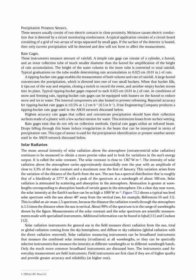
The mean annual intensity of solar radiation above the atmosphere (extraterrestrial solar radiation)continues to be measured to obtain a more precise value and to look for variations in the sun’s energyoutput. It is called the solar constant. The solar constant is close to 1367 W m–2. The intensity of solarradiation above the atmosphere varies approximately sinusoidally over the year with an amplitude ofclose to 3.3% of the solar constant and a maximum near the first of January. This variation arises fromthe variation of the distance of the Earth from the sun. The sun has a spectral distribution that is roughlythat of a blackbody at 5777 K with a peak of the spectrum at a wavelength of about 500 nm. Solarradiation is attenuated by scattering and absorption in the atmosphere. Attenuation is greater at wave-lengths corresponding to absorption bands of certain gases in the atmosphere. On a clear day near noon,the solar intensity at the Earth’s surface can be as high a 1000 W m–2. Figure 73.2 shows a typical sea levelsolar spectrum with the sun about 48° away from the vertical (see, for example, References 10 and 11).This is called an air-mass 1.5 spectrum, because the distance the radiation travels through the atmosphereis 1.5 times the distance when the sun is vertical. About 99% of the spectrum is in the range of wavelengthsshown by the figure. Measurements of the solar constant and the solar spectrum are scientific measure-ments made with specialized instruments. Additional information can be found in Iqbal [11] and Coulson[12].

Solar radiation instruments for general use in the field measure direct radiation from the sun, totalor global radiation coming from the sky hemisphere, and diffuse or sky radiation (global radiation withthe direct radiation removed). Solar radiation measuring instruments can be broadband instrumentsthat measure the combined solar intensity (irradiance) at all wavelengths, or they can be spectrallyselective instruments that measure the intensity at different wavelengths or in different wavelength bands.Only the much more common broadband instruments are discussed here. The instruments used foreveryday measurement are field instruments. Field instruments are first class if they are of higher qualityand provide greater accuracy and reliability (at higher cost).


Direct radiation is radiation coming directly from the sun without scattering in the atmosphere.Instruments measuring direct solar radiation usually include radiation coming from the sky out to anangular distance of about 3° away from the center of the sun’s disk. They are called pyrheliometers. Theradiation coming from clear sky near the sun, rather than from the solar disk, is the circumsolar radiation.This radiation can be subtracted from the pyrheliometer measurement for a more precise determinationof direct radiation. This correction is often not made for routine measurements. The clear sky correctionis calculated using the angular distribution of the intensity of the circumsolar radiation [13,14].

Instruments measuring global radiation are installed in a level position with a plane sensor facing uptoward the sky. These instruments measure solar radiation coming from the whole sky hemisphere. Theyare called pyranometers. Global radiation measuring instruments should be sited in a level elevated areawith no obstructions obscuring the sky hemisphere.

Diffuse radiation is the radiation coming from the sky hemisphere with the direct radiation subtracted.Pyranometers are used for measuring diffuse solar radiation and should be mounted in the same manneras pyranometers used for measurement of global radiation. They have an occulting (shade) disk or shadowband to prevent direct solar radiation from reaching the radiation sensor. The measurement of diffuseradiation involves correcting the pyranometer measurement for the part of the sky radiation shieldedfrom the sensor by the occulting disk or shadow band. For clear skies, the occulting disk correction iscalculated using the angular distribution of intensity of the circumsolar radiation. Corrections for par-tially cloudy and cloudy skies depend on the particular cloud conditions. Corrections for the shadowband are often determined by temporarily replacing the shadow band with an occulting disk when thesky is clear and when it is overcast. Corrections for measurements under other sky conditions can bedetermined by interpolation. The shadow band correction is discussed by LeBaron et al. [15]. Theocculting disk must have a tracking system to make the disk follow the sun over the sky. The shadowband removes solar radiation received from a narrow swath of the sky along the path the sun follows

FIGURE 73.2 The intensity of solar radiation as a function of wavelength for a pathlength through the atmosphereof 1.5 times the vertical path length. The dips in the spectrum are molecular absorption bands.


during the day. The shadow band must be adjusted regularly during the year as the path of the sunchanges over the seasons. The more common solar radiation measuring instruments include the pyra-nometer and pyrheliometer.

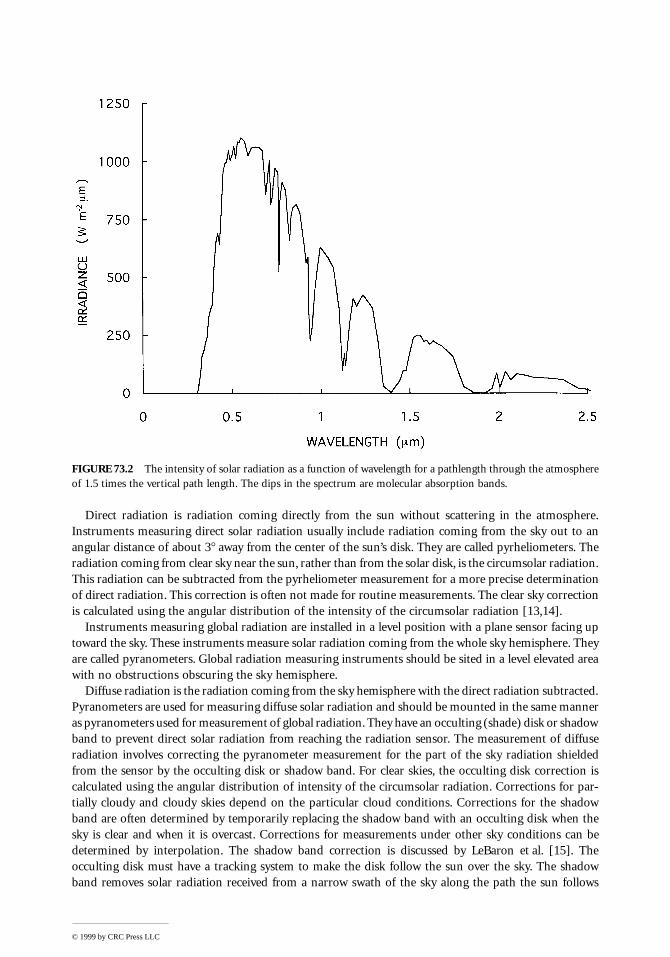
The Pyranometer.The sensor is usually a thermopile, consisting of a number of thermocouples in series, with alternatejunctions heated by the sun. The unheated junctions are near ambient temperature. This is sometimesarranged by putting the unheated junctions in thermal contact with a white surface. Heating by the sunis accomplished by placing the junctions in contact with a matte black surface of high heat conductivityor by a black coating on the junctions. The blackened surface has a constant high solar absorptance(usually ~99%) over the solar spectrum. A constant high solar absorptance over the solar spectrum isimportant. The solar spectrum at the surface of the Earth varies with the time of day and year and theamount of clouds, because of the spectrally dependent scattering and absorption of solar radiation bythe atmosphere. An absorbing surface whose absorption of solar radiation varies with wavelength willcause the sensor to have a different sensitivity for different wavelengths of the solar spectrum. Some lessexpensive pyranometers use a silicon photovoltaic sensor (solar cell) to measure solar radiation. Thesesensors have zero sensitivity above about 1.2 mm and the spectral response below 1.2 mm is not constant.This limits the accuracy of measurements of solar intensity with photovoltaic sensors. Instruments witha thermopile sensor can use a combination of thermopiles and resistors to compensate for the variationof the output of a single thermopile with temperature. The hemispherical windows of pyranometers areusually made of a special glass which transmits solar radiation of wavelengths between about 0.3 and2.8 mm. This includes ~99% of the solar intensity. The absorbing surface must have a cosine response asa function of angle away from the normal to the surface (Lambert law response), and a flat response asa function of azimuth around the normal to the absorbing surface, for the global radiation to be measuredcorrectly. The degree to which the pyranometer response is linear follows the cosine law, and is temper-ature, spectrum, and azimuthally independent, determines whether the instrument is a first class instru-ment. Figure 73.3 shows a Kipp and Zonen (Netherlands) first-class pyranometer.

FIGURE 73.3 A class 1 pyranometer used for the measurement of global and diffuse solar radiation. (Courtesy ofKipp & Zonen Division of Enraf-Nonius Co.)


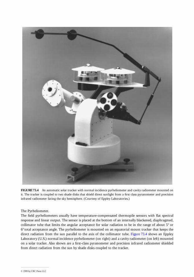
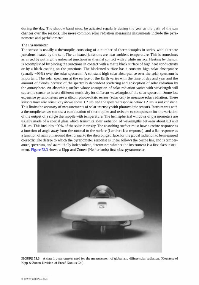
The Pyrheliometer.The field pyrheliometers usually have temperature-compensated thermopile sensors with flat spectralresponse and linear output. The sensor is placed at the bottom of an internally blackened, diaphragmed,collimator tube that limits the angular acceptance for solar radiation to be in the range of about 5° or6° total acceptance angle. The pyrheliometer is mounted on an equatorial mount tracker that keeps thedirect radiation from the sun parallel to the axis of the collimator tube. Figure 73.4 shows an EppleyLaboratory (U.S.) normal incidence pyrheliometer (on right) and a cavity radiometer (on left) mountedon a solar tracker. Also shown are a first-class pyranometer and precision infrared radiometer shieldedfrom direct radiation from the sun by shade disks coupled to the tracker.

FIGURE 73.4 An automatic solar tracker with normal incidence pyrheliometer and cavity radiometer mounted onit. The tracker is coupled to two shade disks that shield direct sunlight from a first class pyranometer and precisioninfrared radiometer facing the sky hemisphere. (Courtesy of Eppley Laboratories.)


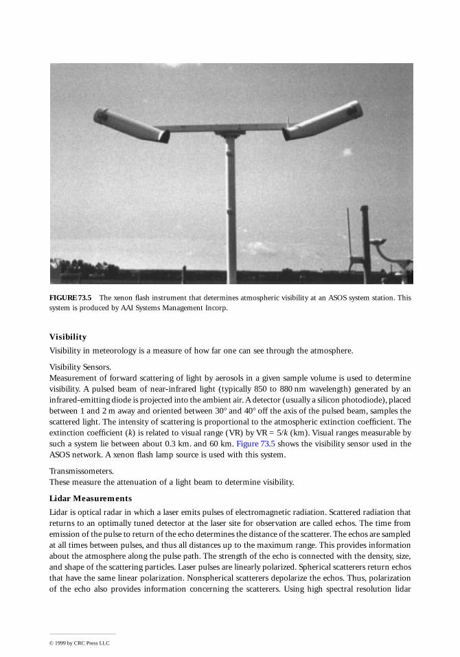
Visibility

Visibility in meteorology is a measure of how far one can see through the atmosphere.

Visibility Sensors.Measurement of forward scattering of light by aerosols in a given sample volume is used to determinevisibility. A pulsed beam of near-infrared light (typically 850 to 880 nm wavelength) generated by aninfrared-emitting diode is projected into the ambient air. A detector (usually a silicon photodiode), placedbetween 1 and 2 m away and oriented between 30° and 40° off the axis of the pulsed beam, samples thescattered light. The intensity of scattering is proportional to the atmospheric extinction coefficient. Theextinction coefficient (k) is related to visual range (VR) by VR = 5/k (km). Visual ranges measurable bysuch a system lie between about 0.3 km. and 60 km. Figure 73.5 shows the visibility sensor used in theASOS network. A xenon flash lamp source is used with this system.

Transmissometers.These measure the attenuation of a light beam to determine visibility.

Lidar Measurements

Lidar is optical radar in which a laser emits pulses of electromagnetic radiation. Scattered radiation thatreturns to an optimally tuned detector at the laser site for observation are called echos. The time fromemission of the pulse to return of the echo determines the distance of the scatterer. The echos are sampledat all times between pulses, and thus all distances up to the maximum range. This provides informationabout the atmosphere along the pulse path. The strength of the echo is connected with the density, size,and shape of the scattering particles. Laser pulses are linearly polarized. Spherical scatterers return echosthat have the same linear polarization. Nonspherical scatterers depolarize the echos. Thus, polarizationof the echo also provides information concerning the scatterers. Using high spectral resolution lidar

FIGURE 73.5 The xenon flash instrument that determines atmospheric visibility at an ASOS system station. Thissystem is produced by AAI Systems Management Incorp.


(HSRL), the scattering by air molecules can be separated from the scattering by aerosols. Differentialabsorption lidar (DIAL) measures the concentration of gaseous species in the atmosphere. Stephens [16]discusses the HSRL and DIAL methods. Zhao et al. [17] present an application of the DIAL method tothe determination of O3 concentration in the atmosphere. Because of their high power output, ruby, dye,neodymium, yttrium-aluminum-garnet (YAG), and CO2 lasers are commonly used for lidar. The use oflidars in the observation of aerosols injected into the stratosphere by volcanic eruption, and theirsubsequent decay has become quite common (see Post et al. [18] and Jager et al. [19] and other articlesin the same journal issue).

Clouds

Observer Estimation.For many years, observers at weather stations have estimated the amount, type, and sometimes the opacityof low clouds, middle clouds, and high clouds. Estimation is usually every hour or similar period withthe estimate in tenths or eighths (octa) of the sky covered. Satellite, radar, and ceilometer data are replacingobserver estimation. Observer estimates have been archived.

Ceilometers.Ceilometers measure the altitude of clouds. Most ceilometers are based on lidar technology using aninfrared pulsed laser diode, usually GaAs. Laser pulses are reflected back (echos) to a receiver, usually aSi diode detector. The round-trip time is converted into cloud height. Common ceilometers can measurecloud base altitudes to 4000 m (12,000 ft). Recent instruments developed by Vaisala can measure cloudbases up to 23,000 m (75,000 ft) with an error of ±1%. The Vaisala ceilometer is used in the ASOSnetwork discussed below. Maintenance includes cleaning of the window. Heaters and blowers respondto automatic sensing units to clear precipitation from the window and control instrument temperature.

Companies producing and marketing meteorological instruments are presented in Table 73.1. Forinformation on additional companies marketing meteorological instruments in the U.S., see ThomasRegister of American manufacturer’s and Thomas Register Catalog File found in most major libraries. Formanufacturers in other countries, search library catalog files under “manufacturers.”

United States Weather Service Facilities

The U.S. National Weather Service, the U.S. Federal Aviation Administration, and the U.S. Departmentof Defense have joined in an upgrade of weather instrumentation and analysis for U.S. weather stations.Other national weather services are upgrading their facilities. The new U.S. National Weather Servicesystem has four components to obtain weather data throughout the United States and its possessions:

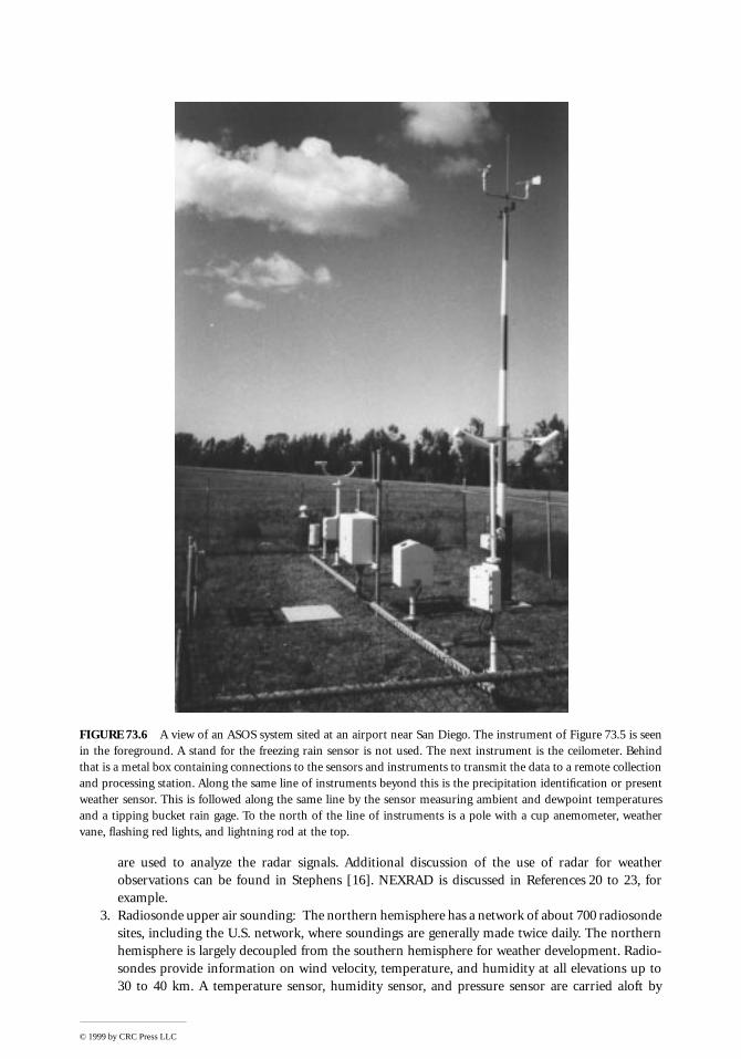
1. The Automated Surface Observing Systems (ASOS): These systems, produced by AAI SystemsManagement Incorporated, are installed at over 850 sites. Each system usually measures visibility,surface temperature, dewpoint temperature, pressure, wind speed and direction, visibility, cloudheight, precipitation identification, freezing rain, and precipitation accumulation. Instrumentsused for each ASOS site are discussed above with other meteorological measuring instruments.Figure 73.6 shows the arrangement of instruments at an ASOS site.

2. Doppler weather surveillance radar (NEXRAD — WSR-88D): Doppler radar are produced byLockheed-Martin Corporation and installed at approximately 160 sites in the U.S. Doppler radarsurveys the weather out to about 300 km from the radar. The standard radar scans angles abovethe horizon up to about 6° in six ~1° intervals with a 360° azimuth. Rain scans go up to about20°. Radar echos are reflection of the pulsed radar microwave signal from water drops in the formof rain or cloud. Ice crystals and snow reflect radar pulses with lower echo strength. Doppler radarcan detect short-lived, possibly catastrophic events such as tornados, downbursts, and flash floodsin real-time. The doppler shift of the echo determines the radial component of the wind velocityat the height and distance of the source of the reflected echo. The strength of the echo providesinformation on the precipitation rate. Powerful computers and sophisticated computer programs


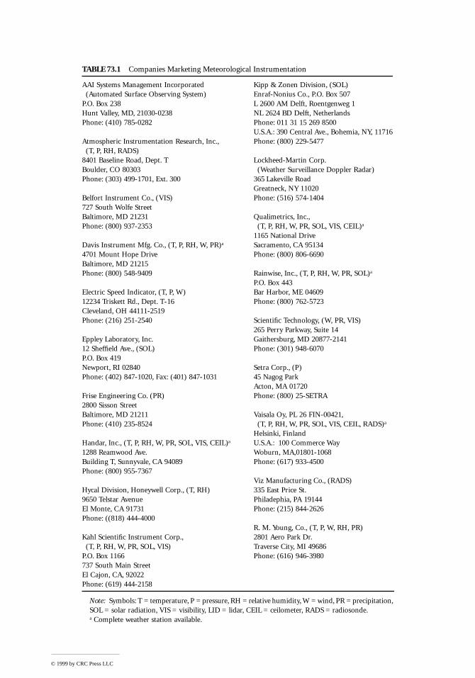
TABLE 73.1 Companies Marketing Meteorological Instrumentation

AAI Systems Management Incorporated (Automated Surface Observing System)

P.O. Box 238Hunt Valley, MD, 21030-0238Phone: (410) 785-0282

Atmospheric Instrumentation Research, Inc., (T, P, RH, RADS)

8401 Baseline Road, Dept. TBoulder, CO 80303Phone: (303) 499-1701, Ext. 300

Belfort Instrument Co., (VIS)727 South Wolfe StreetBaltimore, MD 21231Phone: (800) 937-2353

Davis Instrument Mfg. Co., (T, P, RH, W, PR)a

4701 Mount Hope DriveBaltimore, MD 21215Phone: (800) 548-9409

Electric Speed Indicator, (T, P, W)12234 Triskett Rd., Dept. T-16Cleveland, OH 44111-2519Phone: (216) 251-2540

Eppley Laboratory, Inc.12 Sheffield Ave., (SOL)P.O. Box 419Newport, RI 02840Phone: (402) 847-1020, Fax: (401) 847-1031

Frise Engineering Co. (PR)2800 Sisson StreetBaltimore, MD 21211Phone: (410) 235-8524

Handar, Inc., (T, P, RH, W, PR, SOL, VIS, CEIL)a

1288 Reamwood Ave.Building T, Sunnyvale, CA 94089Phone: (800) 955-7367

Hycal Division, Honeywell Corp., (T, RH)9650 Telstar AvenueEl Monte, CA 91731Phone: ((818) 444-4000

Kahl Scientific Instrument Corp., (T, P, RH, W, PR, SOL, VIS)

P.O. Box 1166737 South Main StreetEl Cajon, CA, 92022Phone: (619) 444-2158

Kipp & Zonen Division, (SOL)Enraf-Nonius Co., P.O. Box 507L 2600 AM Delft, Roentgenweg 1NL 2624 BD Delft, NetherlandsPhone: 011 31 15 269 8500U.S.A.: 390 Central Ave., Bohemia, NY, 11716Phone: (800) 229-5477

Lockheed-Martin Corp. (Weather Surveillance Doppler Radar)

365 Lakeville RoadGreatneck, NY 11020Phone: (516) 574-1404

Qualimetrics, Inc., (T, P, RH, W, PR, SOL, VIS, CEIL)a

1165 National DriveSacramento, CA 95134Phone: (800) 806-6690

Rainwise, Inc., (T, P, RH, W, PR, SOL)a

P.O. Box 443Bar Harbor, ME 04609Phone: (800) 762-5723

Scientific Technology, (W, PR, VIS)265 Perry Parkway, Suite 14Gaithersburg, MD 20877-2141Phone: (301) 948-6070

Setra Corp., (P)45 Nagog ParkActon, MA 01720Phone: (800) 25-SETRA

Vaisala Oy, PL 26 FIN-00421, (T, P, RH, W, PR, SOL, VIS, CEIL, RADS)a

Helsinki, FinlandU.S.A.: 100 Commerce WayWoburn, MA,01801-1068Phone: (617) 933-4500

Viz Manufacturing Co., (RADS)335 East Price St.Philadephia, PA 19144Phone: (215) 844-2626

R. M. Young, Co., (T, P, W, RH, PR)2801 Aero Park Dr.Traverse City, MI 49686Phone: (616) 946-3980

Note: Symbols: T = temperature, P = pressure, RH = relative humidity, W = wind, PR = precipitation,SOL = solar radiation, VIS = visibility, LID = lidar, CEIL = ceilometer, RADS = radiosonde.a Complete weather station available.


are used to analyze the radar signals. Additional discussion of the use of radar for weatherobservations can be found in Stephens [16]. NEXRAD is discussed in References 20 to 23, forexample.

3. Radiosonde upper air sounding: The northern hemisphere has a network of about 700 radiosondesites, including the U.S. network, where soundings are generally made twice daily. The northernhemisphere is largely decoupled from the southern hemisphere for weather development. Radio-sondes provide information on wind velocity, temperature, and humidity at all elevations up to30 to 40 km. A temperature sensor, humidity sensor, and pressure sensor are carried aloft by

FIGURE 73.6 A view of an ASOS system sited at an airport near San Diego. The instrument of Figure 73.5 is seenin the foreground. A stand for the freezing rain sensor is not used. The next instrument is the ceilometer. Behindthat is a metal box containing connections to the sensors and instruments to transmit the data to a remote collectionand processing station. Along the same line of instruments beyond this is the precipitation identification or presentweather sensor. This is followed along the same line by the sensor measuring ambient and dewpoint temperaturesand a tipping bucket rain gage. To the north of the line of instruments is a pole with a cup anemometer, weathervane, flashing red lights, and lightning rod at the top.


balloon at 0000 and 1200 UTC (±1 h). The wind velocity at different altitudes is measured bydetermining the radiosonde position at all times during the flight. The horizontal position of theradiosonde can be obtained by OMEGA, LORAN, or VLF global positioning systems. Additionalinformation on global positioning is found in the section of this handbook on satellite navigationand radiolocation. Pressure can indicate the altitude of the radiosonde. Radar or GPS can measurethe radiosonde position in three dimensions. Radiotheodolites can track the radiosonde to receivethe data transmitted by radio transmitter. The radiosonde manufactured by Viz ManufacturingCo. called Bsonde is used by the U.S. National Weather Service. The instruments are mounted ona lightweight white styrofoam container. The temperature sensor is a thin, 50-mm long rodthermistor painted white to minimize heating by solar radiation. It is mounted outside the con-tainer. It measures temperature to ±0.5°C. The container has an air flow duct for ventilation ofthe relative humidity sensor mounted inside. The relative humidity sensor consists of an insulatingstrip coated with a film of carbon that measures relative humidity from 0 to 100% to ±5%. Thepressure sensor is a nickel, C-span aneroid pressure sensor coupled mechanically to a 180 contactbaroswitch providing the output pressure signal. Pressure is measured from 1060 mb to 5 mb withan accuracy of ±0.5 mb. Sensor signals are sent to the receiving station by an amplitude modulatedtransmitter operating from 1660 to 1700 MHz. The Vaisala Inc. radiosonde sensors used by theU.S. National Weather Service differ from Bsonde by use of a capacitance temperature sensor, acapacitance with polymer dielectric humidity sensor, and a capacitive aneroid pressure sensor.

4. Satellite remote sensing: Meteorological variables are deduced from measurements of the electro-magnetic radiation coming from the atmosphere and the surface of the Earth using satellite basedsensors. Usually, three or more different detector wavelength bands are used. The interpretationis difficult because the electromagnetic radiation can come from many levels of the atmosphereor the Earth’s surface, all at different temperatures, and may have undergone multiple scatteringin the atmosphere and Earth reflection. The energy coming from the atmosphere and the Earth’ssurface is mostly reflected and scattered solar radiation for wavelengths up to about 4 mm. Longerwavelength energy is mostly associated with thermal emission from the Earth and its atmosphere.Thermal emission from the atmosphere and the surface of the Earth consists of overlappingblackbody spectra of different temperatures. Absorption spectra characteristic of various gases inthe atmosphere and their temperatures are superimposed on the overlapping blackbody spectra.Visible wavelengths from about 0.4 mm to 0.7 mm are useful for determining cloud coverage andcloud type. Infrared wavelengths from about 6 mm to 7 mm can be used to determine water vapordensity. Infrared in the range from about 10 mm to 12 mm can be used to look at high clouds. Itis also useful for night observation. Satellite measurements show the motion and development ofthe clouds and storm systems. More detailed discussion is available [16,24-27].

References

1. McGee, T. D., Principles and Methods of Temperature Measurement, New York, John Wiley & Sons,1988.

2. Nicholas, J. V., Traceable Temperatures: An Introduction to Temperature Measurement and Calibra-tion, New York, John Wiley & Sons, 1994.

3. Quinn, T. J., Temperature, New York, Academic Press, 1983.4. Schooley, J. F., Thermometry, Boca Raton, FL, CRC Press, 1986.5. Wilson, R. E., Temperature, In Ross, S. D. (Ed.), Handbook of Applied Instrumentation, Malabar,

FL, Robert E. Krieger Publishing, 1982.6. Hickes, W. F., Humidity and Dew Point, In Ross, S. D. (Ed.), Handbook of Applied Instrumentation,

Malabar, FL, Robert E. Krieger Publishing, 1982.7. Moisture and Humidity Measurement and Control in Science and Industry, Proceedings of the 1985

International Symposium on Moisture and Humidity, Washington, D.C., April 15-18, 1985, ResearchTriangle Park, NC, Instrument Society of America.


8. Silverthorne, S. V., Watson, C. W., and Baxter, R. D., Characterization of a Humidity Sensor thatIncorporates a CMOS Capacitance Measuring Circuit, Sensors and Actuators, 19, 371-383, 1989.

9. Marvin, C. F., Psychrometric Tables for Obtaining the Vapor Pressure, Relative Humidity, and Tem-perature of the Dew Point from Readings of the Wet- and Dry-Bulb Thermometers, Washington, D.C.,U.S. Government Printing Office, 1941.

10. Hulstrom, R., Bird, R., and Riordan, C., Spectral Solar Irradiance Data Sets for Selected TerrestrialConditions, Solar Cells, 15, 365-391, 1985.

11. Iqbal, M., An Introduction to Solar Radiation, New York, Academic Press, 1983.12. Coulson, K. L., Solar and Terrestrial Radiation: Methods and Measurements, New York, Academic

Press, 1975.13. Zerlaut, G. A., Solar Radiation Measurements: Calibration and Standardization Efforts, In Boer,

K. W. and Duffie, J. A. (Eds.), Advances in Solar Energy, Vol. 1, Boulder, CO, American Solar EnergySociety, 1983.

14. Major, G., Circumsolar Correction for Pyrheliometers and Diffusometers, WMKO/TD-NO. 635,Geneva, Switzerland, World Meteorological Organization, 1994.

15. LeBaron, B. A., Michalsky, J. J., and Perez, R., A Simple Procedure for Correcting ShadowbandData for All Sky Conditions, Solar Energy, 44, 249-256, 1990.

16. Stephens, G. L., Remote Sensing of the Lower Atmosphere, Oxford, U.K., Oxford University Press,1994.

17. Zhao, Y., Howell, J. N., and Hardesty, R. M.,Transportable Lidar for the Measurement of OzoneConcentration and Aerosol Profiles in the Lower Troposphere, Atlanta, GA, SPIE InternationalSymposium on Optical Sensing for Environmental Monitoring, SPIE Proceedings, 2112, 310-320,October 11-14, 1993.

18. Post, M., Grund, C., Langford, A., and Proffitt, M., Observations of Pinatubo Ejecta Over Boulder,Colorado by Lidars of Three Different Wavelengths, Geophys. Res. Lett., 19, 195-198, 1992.

19. Jager, H., The Pinatubo Eruption Cloud Observed by Lidar at Garmisch-Partenkirchen, Geophys.Res. Lett., 19, 191-194, 1992.

20. Next Generation Weather Radar: Results of Spring 1983 Demonstration of Prototype NEXRAD Prod-ucts in an Operational Environment, NEXRAD Joint System Program Office, Government Publi-cation R400-N49, September 1984.

21. Next Generation Weather Radar Product Description Document, NEXRAD Joint System ProgramOffice, Government Publication R400-PD-202, December 1986.

22. A Guide for Interpreting Doppler Velocity Patterns, NEXRAD Joint System Program Office, Govern-ment Publication R400-DV-101, October 1987.

23. Heiss, W. H., McGrew, D. L., and Sirmans, D., Nexrad: Next Generation Weather Radar (WSR-88D), Microwave J., 33, 79-80, 1990.

24. Burroughs, W. J., Watching the World’s Weather, Cambridge, U.K., Cambridge University Press,1991.

25. Carleton, A. M., Satellite Remote Sensing in Climatology, Boca Raton, FL, CRC Press, 1991.26. Houghton, J. T., Taylor, F. W., and Rodgers, C. D., Remote Sounding of Atmospheres, Cambridge,

U.K., Cambridge University Press, 1984.27. Scorer, R. S., Cloud Investigation by Satellite, New York, Halsted Press, 1986.

73.2 Air Pollution Measurement

Michael Bennett

There is a huge range of atmospheric pollutants and for a given pollutant there may be a severalcommercially available detection systems. In a document of this size, it is clearly not feasible to discussin detail the theory of operation of every possible system. After some general remarks about air pollutionmonitoring, a broad introduction to the physics of molecular spectroscopy (the most widely used


detection principle) will be presented. The detection of individual pollutants will then be discussed. Mostof the practical examples given will refer to British experience, since this reflects the author’s background.The principles involved, however, are universally applicable. The EPA’s Web site (Table 73.5) provides auseful gateway to American legislation and practice.

Before spending money on a detection system, it is essential that the user understands the purpose ofthe measurement. This will affect both the choice of instruments and the location of monitoring sites.In general, active monitors with short response times will be more expensive than passive, slow-responseinstruments. A survey intended to determine spatial variations of an ambient pollutant might thereforebe best to employ very many cheap, slow-response instruments. A classic example would be currentnational surveys to measure indoor radon pollution. In the U.K., the National Radiological ProtectionBoard (NRPB) will supply householders with two passive detectors, each consisting of a strip of plasticinside a protective container. These are left in a living room and a bedroom for 3 months, at the end ofwhich they are mailed back to the NRPB for analysis. (The number of a-particle trails in the plastic iscounted). The householder is then reassured (or not) as to the safety of the dwelling; the authorities,meanwhile, can build up a national map of Rn concentration in relation to geology, building type, etc.The essence of the system is that the individual detectors are so cheap that the authorities can affordmany thousands, such a number being necessary to provide realistic spatial coverage.

Identification of a particular source in the presence of background emissions, however, requires asensor with a response time of minutes, or 1 h at most, supplemented by meteorological measurements.This need arises because, at temperate latitudes, the wind direction changes by 15° in 1 h and 90° in24 h. Unless a source dominates local pollution, its impact is unlikely to be demonstrable through dailysampling.

Some applications may require response times of seconds or less. Odors are a very common cause ofcomplaint. In this case, the complainant perceives fluctuations in concentration over periods of a fewseconds, while he may become inured to steady concentrations over periods of minutes. It is also thecase that many toxic gases are more damaging in high doses over short periods than at a steady concen-tration over some hours [1]. Flammability, of course, also depends on peak rather than mean concen-trations.

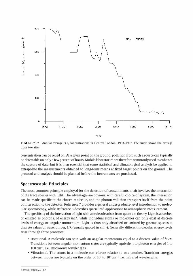
Central to obtaining reliable information from such measurements is the protocol for the siting ofinstruments. This naturally depends on the objectives of the survey. The U.K. national survey for smokeand SO2 [2], for example, was highly successful in demonstrating the effects on background pollutantconcentrations of the 1956 Clean Air Act and (from the late 1960s) the availability of natural gas (cf.Figure 73.7). Sites were chosen so as not to be dominated by individual local sources, being typically inbackyards or on the roofs of municipal buildings. By the early 1980s, however, urban air pollution hadbecome increasingly dominated by road traffic emissions and the earlier network of sites no longer seemedappropriate [3,4]. Many roadside measurements have now also been made in addition to more generalurban or rural surveys [5]. It should be noted that a typical site is not necessarily a representative one[6]. The former is what we experience about our daily lives. The latter is chosen through a protocol sothat measurements from one site can be compared with those from another. Depending on the applica-tion, representative sites may be more or less typical.

A protocol is important not only for comparing one place with another, but also for comparisonsbetween different times. One should not be dismissive of the old technology of the national SO2 survey;the conservatism of the design allows one to rely on the time series of concentrations over the last 60 years.Clearly, there are advantages in keeping up with the latest technology. But, if interested in long-termtrends, one must be very sure of the relative responses of “improved” instruments and methods.

The deployment of fast-response instruments around individual sources gives rise to somewhat dif-ferent problems. Given the high cost of such instruments, one must be sure that statistically usefulmeasurements of environmental impact will be made over the course of the survey. Concentrationsshould ideally be measured simultaneously upwind and downwind of the source. For an elevated buoyantsource, it is desirable to measure downwind concentrations over a range of distances; atmospheric disper-sion models are not yet so foolproof that the calculated distance from the stack to the peak ground-level


concentration can be relied on. At a given point on the ground, pollution from such a source can typicallybe detectable on only a few percent of hours. Mobile laboratories are therefore commonly used to enhancethe capture of data, but it is then essential that some statistical and climatological analysis be applied toextrapolate the measurements obtained to long-term means at fixed target points on the ground. Theprotocol and analysis should be planned before the instruments are purchased.

Spectroscopic Principles

The most common principle employed for the detection of contaminants in air involves the interactionof the trace species with light. The advantages are obvious: with careful choice of system, the interactioncan be made specific to the chosen molecule, and the photon will then transport itself from the pointof interaction to the detector. Reference 7 provides a general undergraduate-level introduction to molec-ular spectroscopy, while Reference 8 describes specialized applications to atmospheric measurement.

The specificity of the interaction of light with a molecule arises from quantum theory. Light is absorbedor emitted as photons, of energy hc/l, while individual atoms or molecules can only exist at discretelevels of energy or angular momentum. Light is thus only absorbed or emitted by gaseous species atdiscrete values of wavenumber, 1/l (usually quoted in cm–1). Generally, different molecular energy levelsarise through three processes:

• Rotational. A molecule can spin with an angular momentum equal to a discrete value of h/2p.Transitions between angular momentum states are typically equivalent to photon energies of 1 to100 cm–1, i.e., microwave wavelengths.

• Vibrational. The atoms in a molecule can vibrate relative to one another. Transition energiesbetween modes are typically on the order of 103 to 104 cm–1, i.e., infrared wavelengths.

FIGURE 73.7 Annual average SO2 concentrations in Central London, 1933–1997. The curve shows the averagefrom two sites.


• Electronic. The electrons can occupy different orbitals within an atom. Transitions between thesewould typically take place at UV wavelengths.

Photons can initiate transitions between combinations of the above levels; observed molecular spectrathus tend to be extremely complicated, having structure over all scales of wavenumber. Atomic spectra,for example, from a monatomic gas like Hg, are simpler, since there are no vibrational or rotationalmodes. Nevertheless, even for molecular spectra, “selection rules” permit only a limited number oftransitions to occur; a single photon can only effect a transition if the initial and final dipole momentsof the molecule are different. (The direction of the change of dipole depends on the polarization of theassociated photon.) Conservation of angular momentum also requires that a molecule’s spin can onlychange by one unit at a time.

Photon energies are broadened by temperature (which causes a Doppler shift in frequency) and bypressure (which shortens the lifetime of the excited state). In practice, of course, any commercial mea-surement system also has a finite resolution. Parts of the spectrum may thus contain so many possibletransitions that it becomes impractical to distinguish individual lines. The specificity of molecule–photoninteractions promised by quantum theory is thus seen to be rather limited in practice. Spectroscopicidentification of a particular species relies on the existence of resolvable structure in an accessible partof the spectrum where there is no serious interference from other common gases. In general, this searchmust be solved individually for each analyte — with no guarantee of the existence of a satisfactorysolution.

Absorption Techniques

Detection of a specific molecule may be through either its absorption or emission of light at a particularwavelength. Consider monochromatic light of flux I passing through a gas of concentration c. In so faras each interaction between a photon and a molecule is an independent event, the rate of interaction isseparately proportional to the number of photons and the number of gas molecules. Thus,

(73.1)

where s(l) is the absorption cross-section. For constant gas concentration, this can be integrated as afunction of path length, x, to give the Beer-Lambert law:

(73.2)

The argument of the negative exponential is known as the optical density at this wavelength. The gasburden, cx, along the optical path is thus given by:

(73.3)

and, since s(l) can be measured in the laboratory, one now has a measurement of the gas concentration.The advantage of absorption techniques is that they require minimal disruption to the observed system.

This is of benefit in ambient monitoring where, for example, a long-path measurement can be set upover many hundreds of meters without problems of safety or power. Equally, in emissions monitoring,it is advantageous to be able to measure gas concentrations in situ in the flue. Long-path techniques canalso be applied in point samplers through the use of a multipass cell (e.g., a White cell [8]). The responsetime would then be limited by the volume of the cell in relation to the sample throughput.

¶ ( )¶

= - ( ) ( ) ( )I x

xI x x

,,

ls l l c

I x I ex

, ,l l s l c( ) = ( ) - ( )0

cl l

s lx

I I x=

( ) ( )( )( )

log , ,0


Because of instrumental offsets and interference from other species, measurement of transmission ata single frequency is unlikely to give an accurate estimate of the gas concentration. More commonly,absorption is measured at several frequencies. Standard techniques include:

• Differential Optical Absorption Spectroscopy (DOAS). A broadband source is used in conjunctionwith a high-resolution spectroscope tuned around distinctive absorption features of the target gas.The difference between online and offline absorption then gives the gas concentration. If themeasured spectrum is digitized, it can be fitted to the target spectrum, allowing some correctionfor interferent species. In a related analog technique, “Correlation Spectrometry,” several onlineand offline signals are taken simultaneously from a spectrometer. Regressing the signal against aknown absorption spectrum using an spectral mask gives the target gas burden.

• Fourier Transform Infrared (FTIR). The output from the gas cell is put into an interferometer.The Fourier transform of the output signal as a function of phase lag is then the absorptionspectrum. Fitting programs can be applied to estimate the mix of pollutants responsible for thisspectrum.

• Non-Dispersive Infrared (NDIR). Optical filters are applied to limit the input spectrum to awindow where interference effects from other gases are small. No further spectral separation(“dispersion”) is then applied. Gross absorption by the target gas is measured and can be calibratedby switching gas cells into the light path.

• TLDAS (Tunable Laser Diode Absorption Spectroscopy). This uses a very narrow-band source(viz. a tunable diode laser) and a broad-band receptor. The frequency of the source will typicallybe oscillated close to an absorption line of the target gas; the first harmonic of the signal is thenproportional to the integrated concentration along the light path.

Emission Techniques

The converse of looking for the absorption of light of a given frequency by the target gas is to excitemolecules of the gas and then examine the light emitted as they return to their ground state. The signalis passed through a narrow-band filter and measured with a photomultiplier tube. There are severalstandard techniques, including:

• Flame photometry. A flame (typically of H2) is burned in the sample gas. The heat breaks up andionizes the target molecules, which then relax to their ground state. Since one is now looking atfragments of the molecule rather than the molecule itself, the technique is not completely specific.Its advantage is that it tends to be very fast, being ultimately limited by the timescale for the ionsto pass through the flame. A related technique, FID (Flame Ionization Detection), although notstrictly spectroscopic, measures the conductivity of the flame that arises from such ionization.

• Chemiluminescence. A reactive gas is added to the sample gas. Light from the excited productsof the reaction is detected.

• UV fluorescence. The sample gas is excited with UV light and the subsequent fluorescence mea-sured. A related technique, PID (Photoionization Detection), is to measure the ionization currentarising from such UV irradiation. This then detects all species whose first ionization potential isless than the photon energy of the lamp. The technique is extremely fast [9].

Particulate Sampling

Sampling of particulate matter in air gives rise to a different set of considerations from the sampling oftrace gases. Note that:

• Spectroscopic methods are unlikely to be effective. The interaction of light with small particles iscaused by Rayleigh or Mie scattering [10] and tends not to show very specific behavior as a functionof particle composition.

• The aerodynamic behavior of a particle is a strong function of its size. Particles of diameter lessthan 10 mm (PM10) tend to travel with the air flow. Since, moreover, their Brownian diffusivity


is very small, they exhibit very slow deposition [11]. At less than 5 mm, such particles may beinhaled deeply into the lungs; as such, they are known as “respirable aerosol.”

• Particles of diameter greater than 10 mm exhibit significant inertial and gravitational effects. Theycan thus deposit through impaction as the air flows around small obstacles. For particles largerthan 50 mm, sedimentation becomes dominant.

The sampling method must thus be tuned to the range of particle sizes that one wants to monitor.For a general review, see the book by Vincent [12].

Slow Ambient Monitoring

The initial discussion focuses on systems with sampling times of 1 day and upward. These would typicallybe used for background monitoring.

Diffusion Tubes

A diffusion tube is the classic inexpensive, slow-response instrument that can be deployed in largenumbers to quantify spatial variations of ambient pollutants. Typically, it consists of a sealed perspextube with a removable cap and an active substrate at the closed end. It is deployed in the field with theopen end downward and, after the prescribed exposure time (typically 7 days) it is returned to thelaboratory for analysis. The system was originally developed as a personal monitor of NO2 exposure [13]but has since been widely used for ambient urban surveys.

Assuming that the substrate is a perfect trap for the target gas, the diffusive flux of gas into the tubeis given by DAc/L, where D is the diffusivity of the target species, A the internal cross-sectional area ofthe tube, and L the length of the tube. So long as the diffusivity remains constant over the period ofmeasurement, the total deposition to the substrate is therefore a measure of the mean concentration overthe period of exposure. Theoretically, D should vary with temperature and there may also be somecirculation within the tube arising from wind across its mouth. A typical commercially available modelhas L = 71 mm and an i.d. of 12 mm, so such circulation is suppressed. Studies have shown acceptablecorrelation between samples from diffusion tubes and long-term means from adjacent point samplers[14].

The system employed for NO2 is a substrate of triethanolamine deposited on a stainless steel mesh.The sample is dissolved in orthophosphoric acid and the nitrite detected colorimetrically using theGreiss/Saltzman technique. Systems are also available for SO2, benzene, xylene, toluene, fluoride, chloride,bromide, cyanide, and nitrate. A list of participating laboratories in the U.K. can be obtained fromNETCen.

Drechsel Bottles

The classic bubbler (a Drechsel bottle) consists of a Pyrex® bottle containing a solution through whichfiltered sample gas is bubbled. Capture of the sample gas can be enhanced by passing it through a sinteredplug, so that bubble size is reduced. For the detection of SO2, a solution of hydrogen peroxide is used sothat:

(73.4)

In polluted areas, the H+ ions are then detected by titration, it being assumed that all the acidity comesfrom atmospheric SO2. In cleaner, rural areas, this is insufficiently sensitive (NH3 emissions from livestockcan give apparently negative SO2 concentrations!) and the sulfate ions are measured using ion chroma-tography. Sampling times are typically 24 h for a sensitivity of a few ppb.

As implemented in the U.K. national surveys of smoke and SO2, eight such bottles are mounted in acase with a separate pump and flowmeter. At some preset time each day, the airflow is switched fromone bottle to the next; at the end of the week, the operator then visits, replaces all the bottles, and returnsthe old ones to the laboratory for analysis. Depending on the time of the visit relative to the switching

H O SO 2H SO2 2 2 42+ ® ++ -


time, the sample on the day of the visit can be spread over two bottles. In this system, the air is firstdrawn through a separate filter (Whatman Grade 1) for each day of measurement. This captures partic-ulate in the range 5 to 25 mm diameter; the blackness of the stain is measured photometrically to providea 24-h sample of “black smoke.”

The system is simple, inexpensive (current list prices are less than $3000), and requires minimaloperator training. It was therefore possible to install many hundreds of such sites and run them for aconsiderable period. In central London, for example, such systems were first installed in 1933. Annualmean SO2 concentrations were then found to be around 400 mg m–3; 60 years later, this has dropped toless than 40 mg m–3. Clearly, there has been considerable improvement. Such measurements have nowbeen considerably scaled down, with 252 sites currently active in the U.K. [5].

In practice, the real cost of such a system is the manpower and the site. These are small if the systemis sited in a municipal building and operated by existing staff. At a remote site, however, a secure cabinwith power must be provided and it must be visited weekly. The practical difficulties of identifying,securing, and maintaining a site should never be underestimated when designing a monitoring network.

Deposition Gages [15]

Traditionally in the U.K., measurements of atmospheric dust have been made using the passive BritishStandard dust deposition gage, while measurements of “smoke” have been made using the active filtersystem described in the previous section. The standard dust deposition gage consists essentially of a bowlof diameter 300 mm and depth 225 mm mounted 1.2 m above the ground; the sample is washed into abottle beneath the gage, from where it is filtered, dried, and weighed. After having been in use for thebetter part of a century, the collection efficiency of the standard gage was tested and found to be, in fact,rather poor. In very light winds, 50% of particulate at 100 mm and 80% at 200 mm might be captured,but these efficiencies fall off very rapidly with increasing wind speed.

More recent work has shown that a gage shaped like an upside-down Frisbee® has a far superiorcapture performance. With the addition of a foam substrate, collection efficiencies in excess of 80% inlight winds, even for particle diameters as small as 50 mm, can be achieved and these efficiencies remaingood at moderate wind speeds. Such gages are now commercially available.

Active Aerosol Sampling

Measurement of particulate matter of aerodynamic diameter less than 100 mm in air requires an activesampling system.

A conventional high-volume sampler for total suspended particulate (TSP) consists of a filter and apowerful blower. The system is mounted in a housing with a pitched roof, the air being drawn in underthe eaves (i.e., at a height of about 1.1 m). Air sampling rates are in excess of 1 m3 min–1. The filter canbe changed and weighed, or otherwise analyzed, after 24 h.

Size discrimination is introduced into such samplers by requiring the air to follow a tortuous path.Small particles then follow the streamlines, while large particles are deposited. As a first stage, the high-volume sampler may have an inlet impaction chamber, which only allows the PM10 fraction to be tocaptured in the filter.

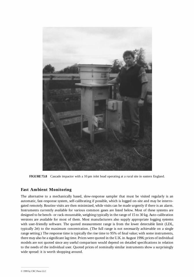
In a more sophisticated system, the filter can be replaced with a cascade impactor. This consists of astack of plates with successively smaller perforations. The holes are staggered so that air passing throughone hole impacts on the following plate. As the perforation size diminishes, the air speed increases andthe size of particle that can escape diminishes. By covering each plate with a removable membrane, theparticulate captured in each size fraction can be analyzed and, in principle, weighed. See Figure 73.8.

Low-flow systems (1 m3 h–1) are also available, which permit measurement of PM10 or PM 2.5. Inletheads, certified by the EPA, are available for various cutoff diameters. Reference 16 quotes captureefficiencies for such devices as a function of particle size.

Active or passive aerosol sampling systems are marketed by, among others, Charles Austin Pumps,Graseby-Andersen, and Casella.


Fast Ambient Monitoring

The alternative to a mechanically based, slow-response sampler that must be visited regularly is anautomatic, fast-response system, self-calibrating if possible, which is logged on-site and may be interro-gated remotely. Routine visits are then minimized, while visits can be made urgently if there is an alarm.Instruments currently available for various common gases are listed below. Most of these systems aredesigned to be bench- or rack-mountable, weighing typically in the range of 15 to 30 kg. Auto-calibrationversions are available for most of them. Most manufacturers also supply appropriate logging systemswith user-friendly software. The quoted measurement range is from the lower detectable limit (LDL,typically 2s) to the maximum concentration. (The full range is not necessarily achievable on a singlerange setting.) The response time is typically the rise time to 95% of final value; with some instruments,there may also be a significant lag time. Prices were quoted in the U.K. in August 1996; prices of individualmodels are not quoted since any useful comparison would depend on detailed specifications in relationto the needs of the individual user. Quoted prices of nominally similar instruments show a surprisinglywide spread: it is worth shopping around.

FIGURE 73.8 Cascade impactor with a 10 mm inlet head operating at a rural site in eastern England.


SO2

Most ambient monitors for SO2 now use UV fluorescence; when irradiated, SO2 molecules re-emit lightin the range 220 to 240 nm. The measured light intensity is then proportional to the SO2 concentration.Currently available systems have response times of order 1 to 4 min, LDL of order 0.5 to 1 ppb, andmaximum ranges of 1 to 100 ppm. Prices start at around $9000. Most manufacturers also supply aconverter that allows H2S to be measured as a separate channel.

NOx

Most ambient monitors for NOx now employ chemiluminescence. Ozone generated within the instru-ment is mixed with the sample air. NO in the sample then reacts very rapidly to form NO2, with theemission of IR radiation (peaking at 1200 nm). This is a first-order reaction. IR emission is thereforeproportional to the NO concentration. Total NOx can be measured by first passing the sample air overa catalytic converter to reduce any NO2 present to NO. By alternating this conversion, or through theuse of a dual channel system, NO2 concentrations may be found by difference. Inevitably, the measure-ment of NO2 will be noisier than that of NO or NOx separately. Currently available systems have responsetimes of order 1 to 4 min, LDL of order 0.5 to 1 ppb, and maximum ranges of 10 to 100 ppm. Pricesstart at around $9000. Most manufacturers also supply a converter that allows NH3 to be measured as aseparate channel.

O3

Most ambient monitors for O3 now use modulated UV absorption. O3 has a broad absorption spectrumin the UV, with a peak around 254 nm. Practical instruments alternate the gas in the absorption cellbetween sample air and a de-ozonized reference gas; from the Beer-Lambert law, the log ratio of thesignal must then be proportional to the O3 concentration. Currently available systems have responsetimes of order 20 s to 2 min, LDL of order 0.5 to 2 ppm, and maximum ranges of 1 to 200 ppm. Pricesstart at around $7000.

CO and CO2

The standard method of measuring ambient CO or CO2 is to use modulated IR absorption (NDIR);modulation of the signal allows detector offsets to be removed. Currently available systems have responsetimes of order 15 s to 2 min, LDL of order 0.05 to 0.1 ppm for CO and <2 ppm for CO2, and maximumranges of 102 to 104 ppm. Prices start at around $9000.

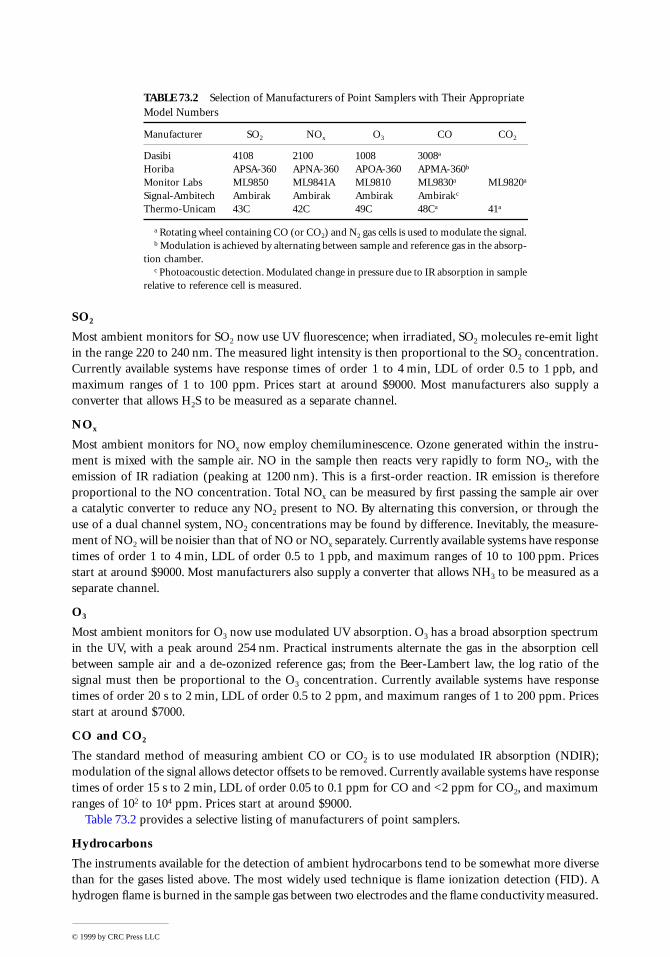
Table 73.2 provides a selective listing of manufacturers of point samplers.

Hydrocarbons

The instruments available for the detection of ambient hydrocarbons tend to be somewhat more diversethan for the gases listed above. The most widely used technique is flame ionization detection (FID). Ahydrogen flame is burned in the sample gas between two electrodes and the flame conductivity measured.

TABLE 73.2 Selection of Manufacturers of Point Samplers with Their Appropriate Model Numbers

Manufacturer SO2 NOx O3 CO CO2

Dasibi 4108 2100 1008 3008a

Horiba APSA-360 APNA-360 APOA-360 APMA-360b

Monitor Labs ML9850 ML9841A ML9810 ML9830a ML9820a

Signal-Ambitech Ambirak Ambirak Ambirak Ambirakc

Thermo-Unicam 43C 42C 49C 48Ca 41a

a Rotating wheel containing CO (or CO2) and N2 gas cells is used to modulate the signal.b Modulation is achieved by alternating between sample and reference gas in the absorp-

tion chamber.c Photoacoustic detection. Modulated change in pressure due to IR absorption in sample

relative to reference cell is measured.


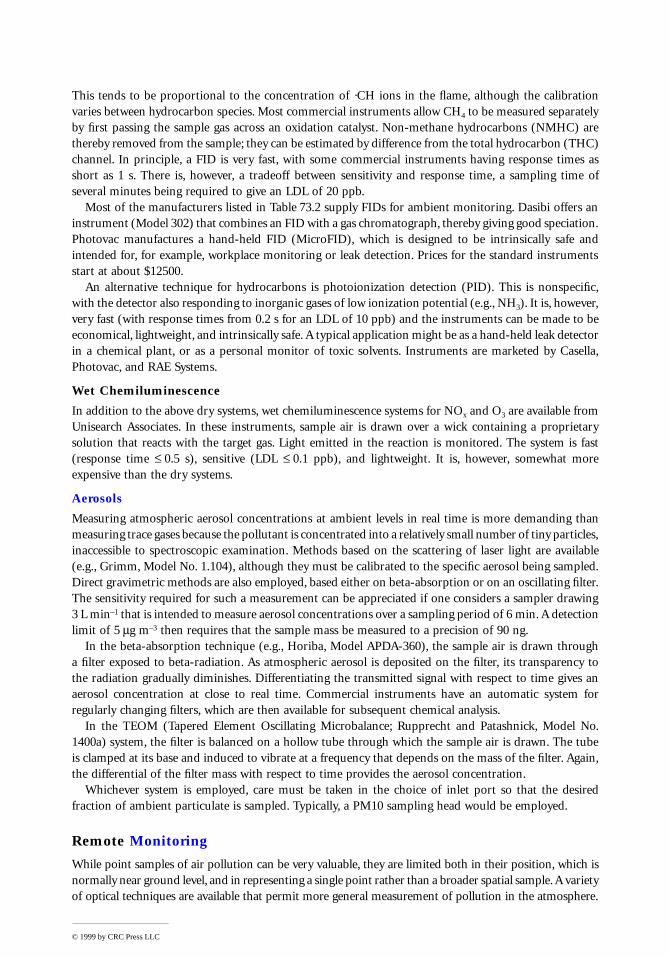
This tends to be proportional to the concentration of ·CH ions in the flame, although the calibrationvaries between hydrocarbon species. Most commercial instruments allow CH4 to be measured separatelyby first passing the sample gas across an oxidation catalyst. Non-methane hydrocarbons (NMHC) arethereby removed from the sample; they can be estimated by difference from the total hydrocarbon (THC)channel. In principle, a FID is very fast, with some commercial instruments having response times asshort as 1 s. There is, however, a tradeoff between sensitivity and response time, a sampling time ofseveral minutes being required to give an LDL of 20 ppb.

Most of the manufacturers listed in Table 73.2 supply FIDs for ambient monitoring. Dasibi offers aninstrument (Model 302) that combines an FID with a gas chromatograph, thereby giving good speciation.Photovac manufactures a hand-held FID (MicroFID), which is designed to be intrinsically safe andintended for, for example, workplace monitoring or leak detection. Prices for the standard instrumentsstart at about $12500.

An alternative technique for hydrocarbons is photoionization detection (PID). This is nonspecific,with the detector also responding to inorganic gases of low ionization potential (e.g., NH3). It is, however,very fast (with response times from 0.2 s for an LDL of 10 ppb) and the instruments can be made to beeconomical, lightweight, and intrinsically safe. A typical application might be as a hand-held leak detectorin a chemical plant, or as a personal monitor of toxic solvents. Instruments are marketed by Casella,Photovac, and RAE Systems.

Wet Chemiluminescence

In addition to the above dry systems, wet chemiluminescence systems for NOx and O3 are available fromUnisearch Associates. In these instruments, sample air is drawn over a wick containing a proprietarysolution that reacts with the target gas. Light emitted in the reaction is monitored. The system is fast(response time £ 0.5 s), sensitive (LDL £ 0.1 ppb), and lightweight. It is, however, somewhat moreexpensive than the dry systems.

Aerosols

Measuring atmospheric aerosol concentrations at ambient levels in real time is more demanding thanmeasuring trace gases because the pollutant is concentrated into a relatively small number of tiny particles,inaccessible to spectroscopic examination. Methods based on the scattering of laser light are available(e.g., Grimm, Model No. 1.104), although they must be calibrated to the specific aerosol being sampled.Direct gravimetric methods are also employed, based either on beta-absorption or on an oscillating filter.The sensitivity required for such a measurement can be appreciated if one considers a sampler drawing3 L min–1 that is intended to measure aerosol concentrations over a sampling period of 6 min. A detectionlimit of 5 mg m–3 then requires that the sample mass be measured to a precision of 90 ng.

In the beta-absorption technique (e.g., Horiba, Model APDA-360), the sample air is drawn througha filter exposed to beta-radiation. As atmospheric aerosol is deposited on the filter, its transparency tothe radiation gradually diminishes. Differentiating the transmitted signal with respect to time gives anaerosol concentration at close to real time. Commercial instruments have an automatic system forregularly changing filters, which are then available for subsequent chemical analysis.

In the TEOM (Tapered Element Oscillating Microbalance; Rupprecht and Patashnick, Model No.1400a) system, the filter is balanced on a hollow tube through which the sample air is drawn. The tubeis clamped at its base and induced to vibrate at a frequency that depends on the mass of the filter. Again,the differential of the filter mass with respect to time provides the aerosol concentration.

Whichever system is employed, care must be taken in the choice of inlet port so that the desiredfraction of ambient particulate is sampled. Typically, a PM10 sampling head would be employed.

Remote Monitoring

While point samples of air pollution can be very valuable, they are limited both in their position, which isnormally near ground level, and in representing a single point rather than a broader spatial sample. A varietyof optical techniques are available that permit more general measurement of pollution in the atmosphere.


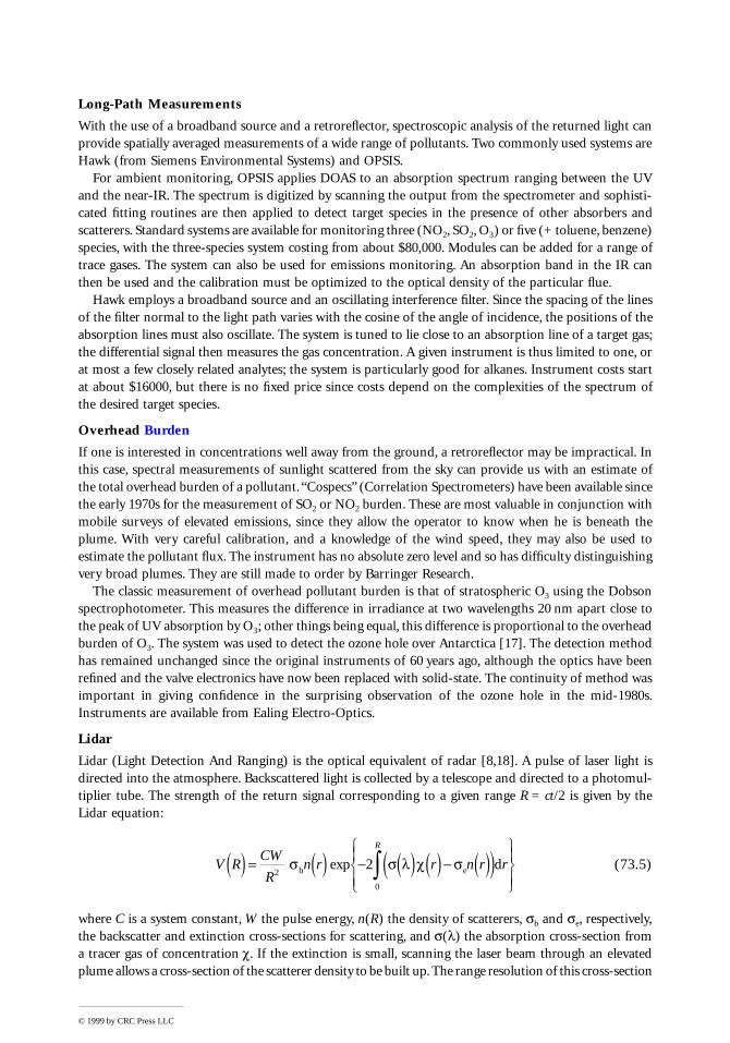
Long-Path Measurements

With the use of a broadband source and a retroreflector, spectroscopic analysis of the returned light canprovide spatially averaged measurements of a wide range of pollutants. Two commonly used systems areHawk (from Siemens Environmental Systems) and OPSIS.

For ambient monitoring, OPSIS applies DOAS to an absorption spectrum ranging between the UVand the near-IR. The spectrum is digitized by scanning the output from the spectrometer and sophisti-cated fitting routines are then applied to detect target species in the presence of other absorbers andscatterers. Standard systems are available for monitoring three (NO2, SO2, O3) or five (+ toluene, benzene)species, with the three-species system costing from about $80,000. Modules can be added for a range oftrace gases. The system can also be used for emissions monitoring. An absorption band in the IR canthen be used and the calibration must be optimized to the optical density of the particular flue.

Hawk employs a broadband source and an oscillating interference filter. Since the spacing of the linesof the filter normal to the light path varies with the cosine of the angle of incidence, the positions of theabsorption lines must also oscillate. The system is tuned to lie close to an absorption line of a target gas;the differential signal then measures the gas concentration. A given instrument is thus limited to one, orat most a few closely related analytes; the system is particularly good for alkanes. Instrument costs startat about $16000, but there is no fixed price since costs depend on the complexities of the spectrum ofthe desired target species.

Overhead Burden

If one is interested in concentrations well away from the ground, a retroreflector may be impractical. Inthis case, spectral measurements of sunlight scattered from the sky can provide us with an estimate ofthe total overhead burden of a pollutant. “Cospecs” (Correlation Spectrometers) have been available sincethe early 1970s for the measurement of SO2 or NO2 burden. These are most valuable in conjunction withmobile surveys of elevated emissions, since they allow the operator to know when he is beneath theplume. With very careful calibration, and a knowledge of the wind speed, they may also be used toestimate the pollutant flux. The instrument has no absolute zero level and so has difficulty distinguishingvery broad plumes. They are still made to order by Barringer Research.

The classic measurement of overhead pollutant burden is that of stratospheric O3 using the Dobsonspectrophotometer. This measures the difference in irradiance at two wavelengths 20 nm apart close tothe peak of UV absorption by O3; other things being equal, this difference is proportional to the overheadburden of O3. The system was used to detect the ozone hole over Antarctica [17]. The detection methodhas remained unchanged since the original instruments of 60 years ago, although the optics have beenrefined and the valve electronics have now been replaced with solid-state. The continuity of method wasimportant in giving confidence in the surprising observation of the ozone hole in the mid-1980s.Instruments are available from Ealing Electro-Optics.

Lidar

Lidar (Light Detection And Ranging) is the optical equivalent of radar [8,18]. A pulse of laser light isdirected into the atmosphere. Backscattered light is collected by a telescope and directed to a photomul-tiplier tube. The strength of the return signal corresponding to a given range R = ct/2 is given by theLidar equation:

(73.5)

where C is a system constant, W the pulse energy, n(R) the density of scatterers, sb and se, respectively,the backscatter and extinction cross-sections for scattering, and s(l) the absorption cross-section froma tracer gas of concentration c. If the extinction is small, scanning the laser beam through an elevatedplume allows a cross-section of the scatterer density to be built up. The range resolution of this cross-section

V RCW

Rn r r n r r

R

( ) = ( ) - ( ) ( ) - ( )( )ìíï

îï

üýï

þïò2

0

2s s l c sb e dexp


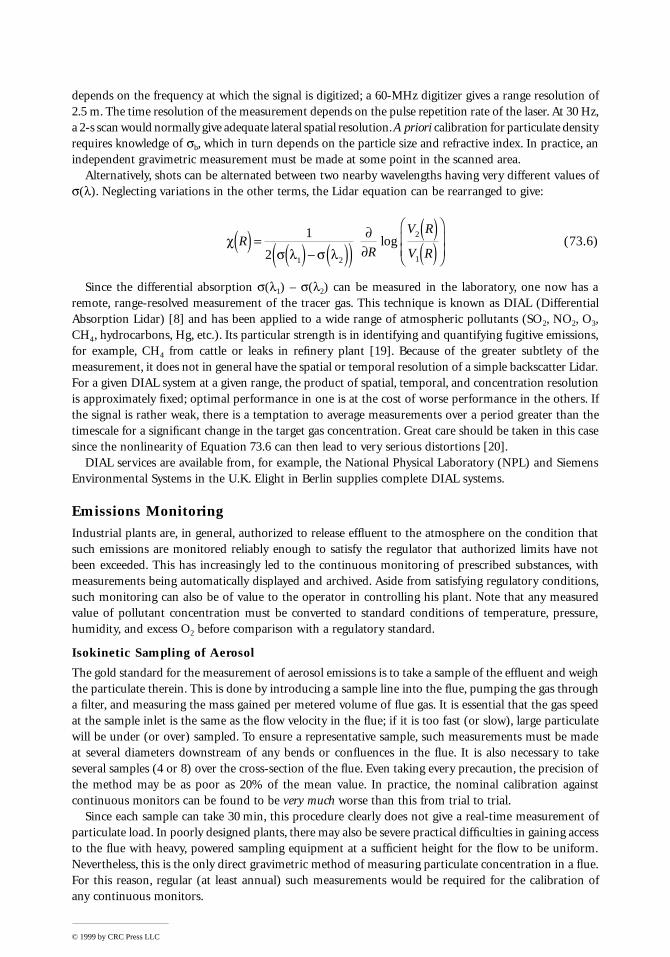
depends on the frequency at which the signal is digitized; a 60-MHz digitizer gives a range resolution of2.5 m. The time resolution of the measurement depends on the pulse repetition rate of the laser. At 30 Hz,a 2-s scan would normally give adequate lateral spatial resolution. A priori calibration for particulate densityrequires knowledge of sb, which in turn depends on the particle size and refractive index. In practice, anindependent gravimetric measurement must be made at some point in the scanned area.

Alternatively, shots can be alternated between two nearby wavelengths having very different values ofs(l). Neglecting variations in the other terms, the Lidar equation can be rearranged to give:

(73.6)

Since the differential absorption s(l1) – s(l2) can be measured in the laboratory, one now has aremote, range-resolved measurement of the tracer gas. This technique is known as DIAL (DifferentialAbsorption Lidar) [8] and has been applied to a wide range of atmospheric pollutants (SO2, NO2, O3,CH4, hydrocarbons, Hg, etc.). Its particular strength is in identifying and quantifying fugitive emissions,for example, CH4 from cattle or leaks in refinery plant [19]. Because of the greater subtlety of themeasurement, it does not in general have the spatial or temporal resolution of a simple backscatter Lidar.For a given DIAL system at a given range, the product of spatial, temporal, and concentration resolutionis approximately fixed; optimal performance in one is at the cost of worse performance in the others. Ifthe signal is rather weak, there is a temptation to average measurements over a period greater than thetimescale for a significant change in the target gas concentration. Great care should be taken in this casesince the nonlinearity of Equation 73.6 can then lead to very serious distortions [20].

DIAL services are available from, for example, the National Physical Laboratory (NPL) and SiemensEnvironmental Systems in the U.K. Elight in Berlin supplies complete DIAL systems.

Emissions MonitoringIndustrial plants are, in general, authorized to release effluent to the atmosphere on the condition thatsuch emissions are monitored reliably enough to satisfy the regulator that authorized limits have notbeen exceeded. This has increasingly led to the continuous monitoring of prescribed substances, withmeasurements being automatically displayed and archived. Aside from satisfying regulatory conditions,such monitoring can also be of value to the operator in controlling his plant. Note that any measuredvalue of pollutant concentration must be converted to standard conditions of temperature, pressure,humidity, and excess O2 before comparison with a regulatory standard.

Isokinetic Sampling of Aerosol

The gold standard for the measurement of aerosol emissions is to take a sample of the effluent and weighthe particulate therein. This is done by introducing a sample line into the flue, pumping the gas througha filter, and measuring the mass gained per metered volume of flue gas. It is essential that the gas speedat the sample inlet is the same as the flow velocity in the flue; if it is too fast (or slow), large particulatewill be under (or over) sampled. To ensure a representative sample, such measurements must be madeat several diameters downstream of any bends or confluences in the flue. It is also necessary to takeseveral samples (4 or 8) over the cross-section of the flue. Even taking every precaution, the precision ofthe method may be as poor as 20% of the mean value. In practice, the nominal calibration againstcontinuous monitors can be found to be very much worse than this from trial to trial.

Since each sample can take 30 min, this procedure clearly does not give a real-time measurement ofparticulate load. In poorly designed plants, there may also be severe practical difficulties in gaining accessto the flue with heavy, powered sampling equipment at a sufficient height for the flow to be uniform.Nevertheless, this is the only direct gravimetric method of measuring particulate concentration in a flue.For this reason, regular (at least annual) such measurements would be required for the calibration ofany continuous monitors.

cs l s l

RR

V R

V R( ) = ( ) - ( )( )

¶¶

( )( )

æ

èçç

ö

ø÷÷

1

2 1 2

2

1

log


Aerosol Sampling: In situ Methods

In situ methods are particularly attractive for emissions measurements because the pollutant is measureddirectly without any possibility of loss or transformation in the path from flue to instrument.

The most obvious way of continuously measuring the dust load in a flue is to pass a beam of lightacross the flue and measure the obscuration. It can be assumed that the transmission obeys the Beer-Lambert law and that the optical density is proportional to the particulate load. Practical instruments,of course, require a degree of sophistication to allow for instrumental offsets. It will not generally bepossible to turn off the plant at regular intervals to check the instrument zero! Typically, the light sourcewill be modulated and a modulated signal measured. Purge air is normally blown over transmitter andreceptor windows (and the retroreflector if used) in order to keep the light path clear. The sensitivity ofthe system will nevertheless drift with time (and will change with the composition of particulate), soregular gravimetric calibration is essential.

Such cross-duct monitors are simple and robust, and they provide a measurement across the full widthof the flue. They are limited to optical densities in the approximate range 0.01 to 2.5. Systems are availablefrom Codel, Land Combustion, Grimm, United Sciences, and others.

For very narrow ducts, or for very low particle densities, a more sensitive technique must be chosen.As with ambient particulate monitoring, it is possible to use sideways scattering from a light beam. Thetransmission and reception optics are now set up so that there is no direct path between the two. Lightscattered from particles in the flue can, however, be detected. This gives a true zero level in the absenceof particulate, and a signal proportional to particle density. Care must be taken to ensure that the lightpath is representative of the particle distribution in the flue. By switching the light path, it might bepossible to route it through a filter of known optical density, thereby permitting online calibration. Suchsystems are available from Erwin-Sick and from United Sciences.

An alternative technique is the triboelectric monitor. In this device, a metal rod is inserted across theflow. Particles striking the rod transfer static charge to it. The leakage current (or, better, the rmscomponent thereof) is thus proportional to the particle flux along the duct. This method is fast, simple,and robust; it is little affected by the accumulation of dirt on the probe and is insensitive to the presenceof steam (which would, of course, preclude optical measurements of particle density). In very wet flows,there are possible problems with leakage across the insulated base of the probe; these can be overcomewith the use of purge air or extended insulation. It should be noted that, with this device, calibration isrequired not only for gravimetric particle density but also for the flow speed in the duct. If this speedvaries significantly, the implicit particle density will be in error. Systems are available from PCME.

Gas Sampling: Spectroscopic Methods

The cross-beam technique can be applied to in situ sampling for pollutant gases. Practical devices areusually based on nondispersive absorption of IR or UV. DOAS can also be used. Sophisticated instru-mental design is necessary to ensure:

• Minimal interference from other species present in the effluent. In combustion gases, for example,high concentrations of H2O, CO2, and acid gases may be present. Measurement of CO in the IRinvolves the use of an absorption window at a wavelength of about 4.7 mm between the absorptionbands of CO2 and H2O.

• Minimal interference from IR emissions from the hot flue gases. Typically, a modulated systemwould be used.

• Insensitivity to instrumental drifts (dirty windows, misaligned optics, aging of source and detec-tor). This can be achieved with dual light-path systems, where only one path is sensitive to thetarget gas. The differential signal then gives a robust measurement of concentration in the flue.This can be calibrated online by switching in cells containing a known concentration of the targetgas.

Table 73.3 provides a selected listing of manufacturers of cross-duct emission systems.


Gas Sampling: Extractive Techniques

If flue gases are to be sampled by an extractive technique, great care must be taken in delivering thesample from the flue to the monitor. Most of the techniques used for extractive emissions monitoringare the same as those for ambient gas monitoring; in many cases, even the same instruments might beused. Since process gases tend to be hotter, wetter, dustier, and more acidic than ambient air, there willoften be a need to change the condition of the sample so that it is acceptable to the monitor. The aimof sampling technology is to deliver an acceptable sample to the instrument at a target gas concentrationthat bears a known relation to the gas concentration in the flue [21].

In general, the sample can be conditioned by dilution, by filtering, by cooling, or by drying. Thetechniques chosen will depend on the gas being measured and on the instrument being used. At itssimplest, conditioning may amount to the sample gas being diluted with several hundred times its volumeof clean air. Normal ambient monitors could then be used, but separate measurements would have tobe made of O2 and H2O in order to express the measured concentration in standard form.

To avoid clogging of the sample line, it is usual to filter the sample as soon as practically possible. Toavoid condensation, the normal practice is to keep the line heated. If, however, the instrument cannottolerate flue gas temperatures, cooling will be necessary at some stage. If this is done without dilution,water will condense out and subsequent measurements will be on a dry gas basis. In itself, this isadvantageous, but any acid gases will remain with the water and be lost. Alternatively, the sample canbe dried by passing it through a permeation drier. Such driers cannot tolerate acid gases. SO2, for example,must therefore be measured on a wet gas basis, with temperature and condensation being controlled byappropriate dilution.

Considerable skill is involved in designing and implementing continuous extractive emissions moni-toring systems. Instruments are available for hydrocarbons and for the conventional range of stack gasesfrom Bernath Atomic (THC), Horiba, Land Combustion, Monitor Labs, Servomex, Signal-Ambitech,and Thermo-Unicam.

Table 73.4 provides the addresses of the various manufacturers of air pollution measurement instru-mentation, and Table 73.5 provides Web site addreses for Table 73.4.

Defining Terms

Aerosol: Particulate matter so finely divided in a gas that it remains in suspension. The aerodynamicdiameter of an aerosol particle is conventionally defined as the diameter of a sphere of density1 g cm–3 which would have the same sedimentation velocity.

Burden: The integrated concentration of an analyte along a defined path.Concentration: The mass or volume of an analyte in a unit sample volume. The volume may need to

be defined in terms of temperature, pressure, humidity etc.Deposition: The transfer of material from the atmosphere to a surface.Monitoring: A routine series of measurements made for control purposes.Protocol: A written list of instructions for obtaining a reliable measurement.

TABLE 73.3 Selection of Manufacturers of Cross-duct Emission Systems

Supplier Technique Gases

Codel NDIR Multigas, CO, SO2, NO/NOx, HCl, H2O, hydrocarbons, NO2, CO2, NH3, VOCsErwin-Sicka DOAS (UV) SO2, NO, NO2, NH3

Land Combustion NDIR COMonitor Labsa NDIR CO, CO2, H2O

Modulated UV NO, SO2

OPSIS DOAS Many

a In these systems, the beam is enclosed within an optical probe inserted into the duct. Sample gas diffuses in througha ceramic filter. Besides protecting the optics, this permits calibration by injecting reference gases into the measurementcavity.


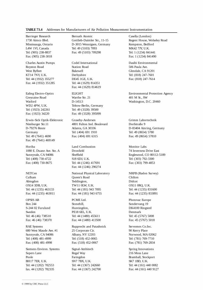
TABLE 73.4 Addresses for Manufacturers of Air Pollution Measurement Instrumentation

Barringer Research1730 Aimco Blvd.Mississauga, OntarioL4W 1Vl, CanadaTel: (905) 238-8837Fax: (905) 238-3018

Bernath AtomicGottlieb-Daimler Str., 11-15D-3015 Wennigsen, GermanyTel: 49 (5103) 7093Fax: 49 (5103) 709298

Casella (London)Regent House, Wolseley RoadKempston, BedfordMK42 7JY, U.K.Tel: 1 (1234) 841441Fax: 1 (1234) 841490

Charles Austin PumpsRoyston RoadWest ByfleetKT14 7NY, U.K.Tel: 44 (1932) 355277Fax: 44 (1932) 351285

Codel InternationalStation RoadBakewellDerbyshireDE45 1GE, U.K.Tel: 44 (1629) 814351Fax: 44 (1629) 814619

Dasibi Environmental506 Paula Ave.Glendale, CA 91201Tel: (818) 247-7601Fax: (818) 247-7614

Ealing Electro-OpticsGreycaine RoadWatfordWD2 4PW, U.K.Tel: (1923) 242261Fax: (1923) 34220

ELIGHTWarthe Str. 21D-14513Teltow-Berlin, GermanyTel: 49 (3328) 39500Fax: 49 (3328) 395099

Environmental Protection Agency401 M St., SWWashington, D.C. 20460

Erwin-Sick Optik-ElektronicNimburger Str.11D-79276 ReuteGermanyTel: 49 (7641) 4690Fax: 49 (7641) 469149

Graseby-Andersen4801 Fulton Ind. BoulevardAtlanta, GA 30336Tel: (404) 691 1910Fax: (404) 691 6315

Grimm LabortechnikDorfstraße 9D-83404 Ainring, GermanyTel: 49 (8654) 5780Fax: 49 (8654) 57810

Horiba1080 E. Duane Ave. Ste. ASunnyvale, CA 94086Tel: (408) 730-4722Fax: (408) 730-8675

Land CombustionDronfieldSheffieldS18 6DJ, U.K.Tel: 44 (1246) 417691Fax: 44 (1246) 290274

Monitor Labs74 Inverness Drive EastEnglewood, CO 80112-5189Tel: (303) 792-3300Fax: (303) 799-4853

NETCenCulhamAbingdonOX14 3DB, U.K.Tel: 44 (1235) 463133Fax: 44 (1235) 463011

National Physical LaboratoryQueen’s RoadTeddington, TW11 0LW, U.K.Tel: 44 (181) 943 7095Fax: 44 (181) 943 6755

NRPB (Radon Survey)ChiltonDidcotOX11 0RQ, U.K.Tel: 44 (1235) 831600Fax: 44 (1235) 833891

OPSIS ABBox 244S-244 02 FurulundSwedenTel: 46 (46) 738510Fax: 46 (46) 738370

PCME Ltd.Stonehill,Huntingdon,PE18 6EL, U.K.Tel: 44 (1480) 455611Fax: 44 (1480) 413500

Photovac EuropeSondervang 19DK4100 RingstedDenmarkTel: 45 (5767) 5008Fax: 45 (5767) 5018

RAE Systems680 West Maude Ave. #1Sunnyvale, CA 94086Tel: (408) 481-4999Fax: (408) 481-4998

Rupprecht and Patashnick25 Corporate Cir.Albany, NY 12203Tel: (518) 452-0065Fax: (518) 452-0067

Servomex Co.Inc.90 Kerry PlaceNorwood, MA 02062Tel: (781) 769-7710Fax: (781) 769-2834

Siemens Environ. SystemsSopers LanePooleBH17 7ER, U.K.Tel: 44 (1202) 782553fax. 44 (1202) 782335

Signal-Ambitech Regal WayFaringdonSN7 7BX, U.K.Tel: 44 (1367) 242660Fax: 44 (1367) 242700

Spring Innovations216 Moss LaneBramhall, StockportSK7 1BD, U.K.Tel: 44 (161) 440 0082Fax: 44 (161) 440 9127


References

1. R.F. Griffiths, The effect of uncertainties in human toxic response on hazard range estimation forammonia and chlorine, Atmos. Environ., 18, 1195-1206, 1984.

2. Warren Spring Laboratory, National Survey of Air Pollution 1961-1971, Vol. 1, ISBN 11 410150 7,London: HMSO, 1972.

3. D.J. Ball and R. Hume, The relative importance of vehicular and domestic emissions of dark smokein Greater London in the mid-1970s, the significance of smoke shade measurements and anexplantation of the relationship of smoke shade to gravimetric measurements of particulate, Atmos.Environ., 11, 1065-1073, 1977.

4. M. Bennett, C. Rogers, and S. Sutton, Mobile measurements of winter SO2 levels in London1983-84, Atmos. Environ., 20, 461-470, 1986.

5. V. Bertorelli and R.G. Derwent, Air quality A to Z: a directory of air quality data for the UnitedKingdom in the 1990s, Meteorological Office, ISBN 0 86180 317 5, 1995.

6. R.E. Munn, The Design of Air Quality Monitoring Networks, London: Macmillan, 1981.7. C.N. Banwell and E.M. McCash, Fundamentals of Molecular Spectroscopy, London: McGraw-Hill,

4th ed., 1994.

Thermo-UnicamP.O. Box 208York StreetCambridgeCB1 2SR U.K.Tel: 44 (1223) 374234Fax: 44 (1223) 374338

United Sciences5310 North Pioneer Rd.Gibsonia, PA 15044Tel: (412) 443-8610Fax: (412) 443-7180

Unisearch Associates222 Snidercroft Rd.Concord, OntarioL4K 1B5, CanadaTel: (905) 669-3547Fax: (905) 669-8652

Note: For reasons of space, only a primary address has been given for each manufacturer. Many of these companieswill have subsidiaries or agents in your own country: a fax should elicit the local address.

TABLE 73.5 Useful Website Addresses for Organizations Listed in Table 73.4

http://www.barringer.com/http://www.bernath-atomic.com/http://www.casella.co.uk/http://www.pentol.com/codel.htmlhttp://www.dasibi.com/http://www.ealing.com/http://www.epa.gov/http://www.elight.de/http://www.sick.de/http://www.graseby.com/http://www.horiba.com/http://www.landinst.com/http://www.monitorlabs.com/http://www.aeat.co.uk/netcen/http://www.npl.co.uk/http://www.pcme.co.uk/http://www.perkin-elmer.com/photo/ (Photovac)http://www.raesystems.com/http://www.rpco.com//index.htm (Rupprecht & Patashnick)http://www.servomex.com/http://www.siemens.co.uk/http://www.spring-innovations.co.uk/http://www.unicam.co.uk/

TABLE 73.4 (continued) Addresses for Manufacturers of Air Pollution Measurement Instrumentation


8. M.W. Sigrist (Ed.), Air Monitoring by Spectroscopic Techniques, New York: Wiley-Interscience, 1994.9. R. F. Griffiths, I, Mavroidis, and C.D. Jones, The development of a fast-response portable photo-

ionization detector: a model of the instrument’s response and validation tests in air, J. MeasurementSci. Technol., 8, 1369–1379, 1998.

10. H.C. van de Hulst, Light Scattering by Small Particles, New York: Wiley, 1957.11. J.H. Vincent, Aerosol Sampling. Science and Practice, New York: John Wiley & Sons, 1989.12. G.A. Sehmel, Particle and gas dry deposition: a review, Atmos. Environ., 14, 983-1011, 1980.13. E.D. Palmes, A.F. Gunniston, J. DiMattio, and C. Tomczyk, Personal sampler for nitrogen dioxide,

J. Amer. Ind. Hyg. Assoc., 37, 570-577, 1976.14. G.W. Campbell, J.R. Stedman, and K. Stevenson, A survey of nitrogen dioxide concentrations in

the United Kingdom using diffusion tubes, July-December 1991, Atmos. Environ., 28, 477-486,1994.

15. D.J. Hall, S.L. Upton, and G.W. Marsland, Designs for a deposition gage and a flux gage formonitoring ambient dust, Atmos. Environ., 28, 2963-2979, 1994.

16. D. Mark and D.J. Hall, Recent developments in airborne dust monitoring, Clean Air, 23, 193-217.17. J.C. Farman, B.G. Gardiner, and J.D. Shanklin, Large losses of total ozone reveal seasonal ClOx/NOx

interactions, Nature, 315, 207-210, 1985.18. D.J. Carruthers, H. Edmunds, M. Bennett, P.T. Woods, M.J.T. Milton, R. Robinson, B.Y. Under-

wood, and C.J. Franklin, Validation of the UK-ADMS dispersion model and assessment of itsperformance relative to R-91 and ISC using archived Lidar data, Dept. of the Environment, ResearchReport No. DOE/HMIP/RR/95/022, March 1996.

19. R.H. Partridge, P.T. Woods, M.J.T. Milton, and A.J. Davenport, Gas standards and monitoringtechniques for measurements of vehicle and industrial emissions, occupational exposure and airquality, Monitor ’93, 23-35, Manchester: Spring Innovations Ltd., 1993.

20. M. Bennett, The effect of plume intermittency upon differential absorption Lidar measurements,Atmos. Environ., 32, 2423-2427, 1998.

21. K. Honner, Continuous extractive gaseous emissions monitoring, Monitor ’93, 53-56, Manchester:Spring Innovations Ltd., 1993.

73.3 Water Quality Measurement

Kathleen M. Leonard

Maintaining and verifying water quality is important in many environmental applications. The mostobvious is in drinking water applications; but industrial and municipal wastewater, natural sur-face/groundwater, industrial process waters, and closed-loop control systems all require a certain rangeor maximum concentration of species to operate properly. Therefore, the development of instrumentationfor monitoring and detecting these contaminants is a highly competitive area. Of course, the chemicalspecies of interest depend on the ultimate use of the water, but this chapter section deals with some ofthe water quality sensors and instrumentation being currently used.

Table 73.6 provides a list of the most commonly monitored chemical species in the area of waterquality. The third column categorizes the parameters in the general categories of drinking water, waste-water (municipal), industrial, stormwater, and ambient water quality. The “ultimate reference” sourcefor accepted methods of determining chemical concentrations in water is known as the Standard Methodfor the Examination of Water and Wastewater [1]. This book has been updated regularly since 1905 andcontains the current techniques recommended by Water Environment Federation (WEF) and the U.S.Environmental Protection Agency (EPA).

The next chapter subsection introduces the theory behind the some of the major types of water qualitysensors, including electrical, optical, and chemical separation. Since each technique has its own particularwater quality applications, a brief discussion of advantages and disadvantages is included. This sectionis limited to commercially available instruments commonly used both inside and outside the laboratory,


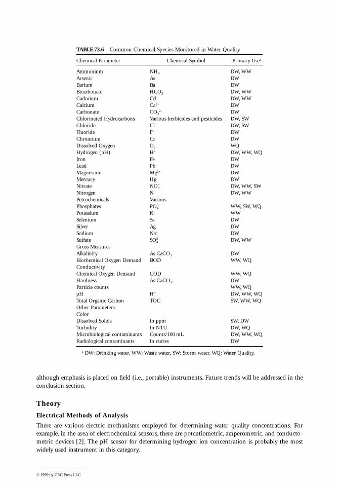
although emphasis is placed on field (i.e., portable) instruments. Future trends will be addressed in theconclusion section.

Theory

Electrical Methods of Analysis

There are various electric mechanisms employed for determining water quality concentrations. Forexample, in the area of electrochemical sensors, there are potentiometric, amperometric, and conducto-metric devices [2]. The pH sensor for determining hydrogen ion concentration is probably the mostwidely used instrument in this category.

TABLE 73.6 Common Chemical Species Monitored in Water Quality

Chemical Parameter Chemical Symbol Primary Usea

Ammonium NH4 DW, WWArsenic As DWBarium Ba DWBicarbonate HCO3

– DW, WWCadmium Cd DW, WWCalcium Ca2+ DWCarbonate CO3

2– DWChlorinated Hydrocarbons Various herbicides and pesticides DW, SWChloride Cl– DW, SWFluoride F– DWChromium Cr DWDissolved Oxygen O2 WQHydrogen (pH) H+ DW, WW, WQIron Fe DWLead Pb DWMagnesium Mg2+ DWMercury Hg DWNitrate NO3

– DW, WW, SWNitrogen N DW, WWPetrochemicals VariousPhosphates PO4

3– WW, SW, WQPotassium K+ WWSelenium Se DWSilver Ag DWSodium Na+ DWSulfate SO4

2– DW, WWGross MeasuresAlkalinity As CaCO3 DWBiochemical Oxygen Demand BOD WW, WQConductivityChemical Oxygen Demand COD WW, WQHardness As CaCO3 DWParticle counts WW, WQpH H+ DW, WW, WQTotal Organic Carbon TOC SW, WW, WQOther ParametersColorDissolved Solids In ppm SW, DWTurbidity In NTU DW, WQMicrobiological contaminants Counts/100 mL DW, WW, WQRadiological contaminants In curies DW

a DW: Drinking water, WW: Waste water, SW: Storm water, WQ: Water Quality.


Potentiometric Sensors.This type of sensor is based on the relationship of the electrochemical cell and the chemical activity ofa sample, based on the general form of the Nernst equation:

(73.7)

for the general reaction: ox + ne– « red. ox and red indicate the oxidized and reduced species [3]. Theterm RT/F has a value of 0.059. E0 is the standard cell potential and Ecell is the adjusted cell potential. Inshort, the activities of the oxidized and reduced species determine the potential of the electrode. If therelationship of the reacting species is known, it is used to measure concentration of that species in anothersolution. In most electrochemical instruments, it is important to maintain a reference electrode whosepotential remains constant for all cell conditions or one that can be easily calibrated for other species.These sensors are commonly known as ion-selective electrodes (ISE) in environmental applications (alsoknown as ion-sensitive field-effect transistors or ISFET). They are all based on the activity level of aspecific ion within a solution. The key to the ISE is the use of an ion-specific membrane with channelsize proportional to the concentration of the ion. It is necessary to maintain a reference potential toensure that the “ion concentration will be directly related to the substrate potential [4].” Specific electrodescan be based on a gas electrode, metal electrode, oxidation–reduction electrode, membrane electrode,glass, liquid membrane, crystalline membrane, or electrode with metal contacting a slightly soluble salt[5]. Examples of this type of sensor and instrumentation for gross measurements include pH sensors,dissolved oxygen, hardness, and dissolved solids.

Commercially available ion-selective electrodes include sensors for ammonia, chlorides, cyanide,iodide, fluoride, nitrates, potassium, and sodium. The instruments labeled as multiparameter waterquality monitors, such as that available from Solomat, are usually composed of one meter with separateprobes for each measurement parameter. However, some of these multiparameter monitors have beenupgraded with a multichannel probe that contains the separate probes within a single housing.

A membrane probe in popular usage is the dissolved oxygen probe based on the principle of polarography.It consists of a gas-permeable membrane over a silver anode and a platinum cathode within a cavity fullof electrolyte (usually KCl). Figure 73.9 shows the placement of the anode and electrode in a typicalpolarographic membrane probe. Since the oxygen will be reduced at the cathode, a current is induced. Theamount of oxygen can then be correlated to the current when a potential is applied to the anode and cathode.

The pH instrument is one of the most commonly used potentiometric sensors in water qualityapplications. It is based on a glass electrode that develops a potential related to hydrogen ion activity ofthe solution. Since this probe was initially developed in the early part of the 1900s, there are numerousprobes and meters on the market. Small, battery-operated, hand-held units are excellent choices forfieldwork. However, for more precise applications, advanced (i.e., expensive) laboratory-grade instru-ments are also available. Most pH probes require standardization and may have other upkeep require-ments after prolonged usage.

Amperometric Sensors.The amperometric classification of electrical sensors is based on the measurement of current through aworking electrode. An empirical relationship can be used to enhance the performance of these electrodes.An example of such a probe is an electrode for chlorine, consisting of a silver anode and platinum cathodewithin an electrolyte reservoir. A chemically specific membrane allows only the ions of interest withinthe probe cavity near the cathode. Reduction occurs at the cathode and then the silver anode reacts withthe electrolyte and, through oxidation, positively charged ions produce a current.

Conductometric Sensors.The conductometric sensors are based on measurements of concentration of a sample due to modulationin conductivity. For example, conductivity is usually measured with a direct reading of electricalconductivity in water, which is then correlated with the number of ions present. The probe usually

E E RT nFcell red ox= - ( ) ( ) ( ){ }0 ln


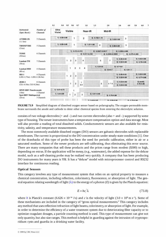
consists of two voltage electrodes (+ and –) and two current electrodes (also + and –) supported by sometype of housing. The newer instruments have a temperature compensation option and data storage. Mostwill also provide a reading of total dissolved solids. Conductometric sensors are also available for resis-tivity, salinity, and temperature measurements.

The most commonly available dissolved oxygen (DO) sensors are galvanic electrodes with replaceablemembranes. The current is proportional to the DO concentration under steady-state conditions [1]. Oneof the drawbacks of this type of probe has been the need for periodic calibration, either in air or asaturated medium. Some of the newer products are self-calibrating, thus eliminating this error source.There are many companies that sell these products and the prices range from modest ($300) to high,depending on extras. If the application will be messy, (e.g., wastewater), the added expense for the deluxemodel, such as a self-cleaning probe may be realized very quickly. A company that has been producingDO instruments for many years is YSI. It has a “deluxe” model with microprocessor control and RS232interface for continuous reading.

Optical Sensors

This category involves any type of measurement system that relies on an optical property to measure achemical concentration, including reflection, colorimetry, fluorescence, or absorption of light. The gen-eral equation relating wavelength of light (l) to the energy of a photon (E) is given by the Planck equation:

(73.8)

where h is Planck’s constant (6.626 ´ 10–34 J s) and c is the velocity of light (3.0 ´ 108 m s–1). Some ofthese mechanisms are included in the category of “gross optical measurements.” This category includesany method that uses reflection/refraction of light beams, colorimetry, or absorption of light. For example,in order to determine the efficiency of a water treatment system due to deteriorating filter capacity or tooptimize coagulant dosages, a particle counting method is used. This type of measurement can give notonly quantity, but also size ranges. This method is helpful in guarding against the intrusion of cryptospo-ridium cysts and guardia in a drinking water facility.

FIGURE 73.9 Simplified diagram of dissolved oxygen sensor based on polarography. The oxygen-permeable mem-brane surrounds the anode and cathode to deter other chemical species from entering the electrolytic solution.

E hc= l


Nephelometry.In this method, light is directed to the sample and the light reflected at right angles to the beam ismeasured (Tyndall effect). This type of analysis is the accepted method for quantifying turbidity (cloud-iness) since the intensity of light scattered by a water sample can be compared to the scattering of astandard (usually Formazin polymer) under similar conditions. The units measured are known asnephelometric turbidity units (NTUs), which are approximately comparable to the older “candle” units.A turbidimeter consists of a light source and a photoelectric sensor that measures the light scattered at90° from the source.

Absorbance Methods.Certain chemical species exhibit natural light absorbance patterns over a range of wavelengths. Theseinclude nitrates/nitrites, heavy metals, unsaturated organics, and aromatics. This approach is valid evenin multicontaminant solutions, since no two substances have exactly the same absorbance pattern. Severalcommercially available instruments take this technology to water quality applications with online capa-bilities. For example, in the water/wastewater area, there are flow-through monitors that measure a broadrange of wavelengths of ultraviolet light simultaneously. This pattern is checked against a “signature” forthe contaminant of interest and both the presence and concentration are verified.

Some contaminants do not have a natural absorbance, so a “conditioning” step is required in orderto use this method. This usually involves the addition of a secondary chemical, or indicator, that willabsorb in the presence of the contaminant. This is commonly known as induced light absorbance.Ammonia, phosphates, and chlorine absorbance probes are available with this conditioning step.

There are several advantages to using absorbance, including low maintenance, especially when com-pared to ISEs, high reliability, and automatic compensation for turbidity (which can cause havoc in othersystems). One of the major drawbacks of the available models is the need to buy a separate unit for eachcontaminant, at a comparatively higher cost than ISE.

Colorimetry.This simple method works by correlating the color of a solution with the concentration of a specificchemical. The theory is that light absorption (A), which is the amount of light intensity (I/I0) absorbed,as is related to concentration based on Beer’s Law [5]:

(73.9)

where kn is the constant for a particular solution and C is the concentration of the solution. Beer’s lawis valid for most water quality ranges of concentration, but it can be verified using dilutions of a specificcontaminant. The first and still simplest colorimetric methods involve the use of color-comparitor tubes(or Nessler tubes) for comparing a range of standards to water samples. However, this method issusceptible to large discrepancies due to human error in selecting variations of tints of a color. Aninstrument that improves upon the accuracy of colorimetry is a photoelectric colorimeter. A light sourceis directed through a filter (making it monochromatic), then passed through the sample cell and on tothe photoelectric detector. The obvious advantage over the comparitor is the elimination of the humanfactor for identifying variations in color. Another adaptation is the spectrophotometer, which employsa diffraction grating to select the wavelength for a wide variety of uses. It is a very versatile instrumentsince both the incoming and outgoing wavelengths are selectable. Newer models incorporate computerchips for automatic programming and data storage.

Colorimetric tests include single analyte meters for chlorine and DO, and direct readout multianalytephotometers for many parameters. For example, the DPD colorometric method is commonly used tomeasure total chlorine concentrations in water and wastewater. However, it must be used with caution,since turbidity, other organic contaminants, monochloromine, etc. will cause interference.

A I I k Cn= ( ) =log 0


Fluorimetry.This method utilizes the fluorescence, either natural or induced, of a compound. Fluorescent chemicalsabsorb radiation of a specific wavelength and emit at another. Fluorescent tracers are commonly used inwater quality studies to determine direction of flow for both surface and groundwater systems. Fluorescenttracers include Rhodamine B, Fluorescein, and Pontacyl Pink B. The detection instrument is known asa fluorimeter, which range from moderate cost for a stationery (single chemical) wavelength model(<$4000) to high cost for a unit with variable wavelength and detection capabilities.

Remote Fiber-Optic Spectroscopy.In the area of in situ chemical analysis, remote fiber spectroscopy (RFS) shows much promise for a varietyof monitoring applications. RFS is a fiber-optic application of existing spectroscopic techniques that canbe applied to the monitoring of chemical species in remote locations. In this method, light of anappropriate frequency is launched into a single optical fiber or fiber bundle. The light is guided to theregion of interest through the fiber by the mechanism of total internal reflection. An optical sensor(optrode) designed for a specific chemical or chemical group is positioned at either the distal end of thefiber, or a length along the fiber. The altered signal is returned through the same fiber to the spectrometerfor signal decoupling and analysis. The major advantages to fiber-optic chemical sensors (FOCS) includetheir small diameter, in situ nature, resistance to harsh environments, and imperviousness to electricinterference. These properties make FOCS ideal for many environmental applications.

The distinguishing feature of most RFS systems is the type of sensor employed. There are basicallytwo approaches to the sensor, either intrinsic or extrinsic. The intrinsic method utilizes the fiber itselfas the active element, for example, using change in index of refractions from the fiber to the media asthe parameter being measured. The extrinsic method uses the fiber optic only as light pipe, and usuallyinvolves incorporating a chemical onto the fiber as the active element. Most of the related literature forfiber-optic chemical sensors (FOCS) deals with design and advantages of various types of optrodes, thatexploit either absorbance, surface enhanced Raman scattering, or fluorescence. Although FOCS havebeen mentioned in literature for the past decade, there has been little success in developing a multicon-taminant sensor for practical applications.

The direct fluorescence approach (measuring the natural fluorescence of the media) is an attractivetechnique for applications where aromatic chemicals are to be monitored. However, since many chemicalsthat act as contaminants are nonfluorophores, a fluorescent intermediate can be incorporated in theFOCS. Ideally, the intermediate should be sensitive to either a group of chemicals or a specific compound,and exhibit a spectral response that could be exploited to identify the compound.

As mentioned previously, the standard pH instrumentation is based on a glass pH electrode; however,optical methods have obvious advantages in corrosive conditions and fluctuating temperatures [6].Optical-based pH sensors are generally based on the changes in the absorbance or fluorescence of anindicator dye that has been immobilized on a fiber optic. Recently, pH sensors based on the immobili-zation of flurorescein dye in a sol-gel matrix have been developed. Sol-gel chemistry is a method ofproducing a porous glass matrix at a low temperature using a hydroloysis of an alkoxide (usually TEO).An example of such a probe is a pH probe based on fluorescein dye in a sol-gel matrix [7].

Optical sensors for O2 and dissolved oxygen, which are based on fluorescence or phosphorescencequenching, have the advantage of size, nonconsumption of oxygen, and resistance to interference due toflow rates or sample stirring over traditional dissolved oxygen electrodes. The major limitations is findingan indicator dye with a strong sensitivity to oxygen quenching. There are many such studies beingperformed; however, most are still in the research stage. For example, polycyclic aromatic hydrocarbonssuch as pyrene and long-wave absorbing dyes have been investigated due to their ability to be quenchedby oxygen [6]. A fiber optics-based sensor that is on the market detects VOCs, such as carbon tetrachlo-ride, TCE, and BTX in water systems (FiberChem). A similar application is a fluorescence-based systemfor measuring petroleum products in the groundwater.


Other Sensors

Infrared Spectrophotometry.Most organic chemical compounds exhibit absorption in the infrared. This attribute can be used todetermine atomic groupings based on quantum mechanics [5]. An example is a unit that measures totalorganic content (TOC) using UV-promoted persulfate oxidation and nondispersive infrared detection.This methodology allows for online TOC monitoring. Correlations can be made to convert values ofTOC to biochemical oxygen demand (BOD) and chemical oxygen demand (COD) for particular samples.Drawbacks to this method include pretreatment to remove inorganic carbon and the high cost ofinstrumentation.

Respirometry.The standard method to calculate BOD5 is to measure oxygen consumption (based on DO concentration)over a 5-day period. However, there are other respirometers based on extremely small differences in DOor CO2 concentrations using external gas sensors. This method is great for respirometry rates of animals,biodegradable contaminants, and sediment oxygen demand studies.

Chemical Separation Techniques

Separation techniques are based on the phase partitioning of molecules within a mixture. Gas chroma-tography refers to a mobile phase of a vapor, while liquid chromatography refers, of course, to a liquidmobile phase. There are several commonly used types such as gas-liquid chromatography, high-perfor-mance liquid chromatography (HPLC), and ion chromatographs. An excellent reference book for thesemethods is Chemistry for Environmental Engineering [5]. The advantages of these instruments are theability to detect components in complex mixtures and high sensitivity. Chromatography instrumentshave long been considered standard in environmental laboratories, but the size of the instruments hasbeen a drawback for field applications. However, size constraints are being challenged with the availabilityof equipment with size reductions of over 90%.

Mass Spectrometry.In environmental applications, these are usually used in conjunction with gas chromatography and arereferred to as GC/MS. The attraction of these instruments is the ability to detect a variety of compoundsand also determine the mass fragmentation patterns of a complex organic structure [1]. The MS essentiallyionizes the substances with an electron beam. The ions are then accelerated through a series of lensesaccording to their mass-to-charge ratios. The charged fragments are detected by a electron multiplier, whichresults in a mass spectra for the particular compound. In addition to the old-fashioned lab-scale GC/MS,there are portable units now commercially available that can be taken into the field for on-site environmentalcharacterizations. These are very useful for ambient air toxics analysis, process diagnostics, and “real-time”groundwater plume movement. However, a newer technique of capillary electrophoresis (CE) has beengaining in popularity over capillary GC since it requires less solvent and can be extremely sensitive.

Atomic Absorption Spectrometry.Since metals have their own characteristic absorption wavelengths, they are usually measured by theatomic absorption method where a light beam is directed into a sample being aspirated onto a flame.The resulting light is then sent to a monochromator with a detector that measures the amount of lightabsorbed by the flame. This method exhibits high sensitivity and is applicable to all of the commonlyfound metals in water. The drawback of this type of instrument is that it is not portable and is more ofa laboratory method.

Instrumentation and Applications

Table 73.7 lists some of the instruments that are commercially available for specific water applications.This is not an exhaustive list of all types and manufacturers, but is indicative of the chemical parameters


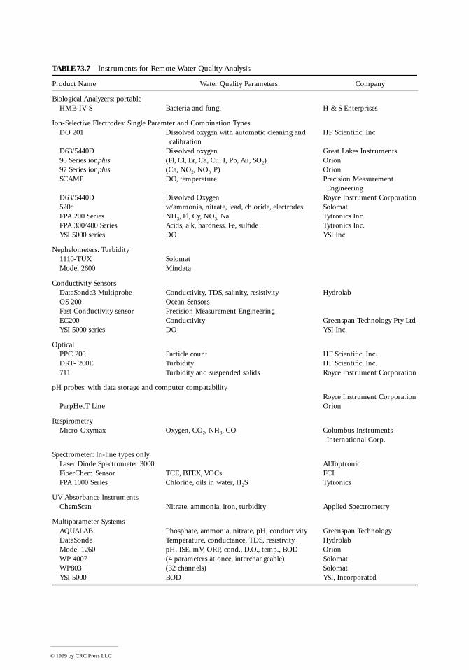
TABLE 73.7 Instruments for Remote Water Quality Analysis

Product Name Water Quality Parameters Company

Biological Analyzers: portableHMB-IV-S Bacteria and fungi H & S Enterprises

Ion-Selective Electrodes: Single Paramter and Combination TypesDO 201 Dissolved oxygen with automatic cleaning and

calibrationHF Scientific, Inc

D63/5440D Dissolved oxygen Great Lakes Instruments96 Series ionplus (Fl, Cl, Br, Ca, Cu, I, Pb, Au, SO2) Orion97 Series ionplus (Ca, NO2, NO3, P) OrionSCAMP DO, temperature Precision Measurement

EngineeringD63/5440D Dissolved Oxygen Royce Instrument Corporation520c w/ammonia, nitrate, lead, chloride, electrodes SolomatFPA 200 Series NH3, Fl, Cy, NO3, Na Tytronics Inc.FPA 300/400 Series Acids, alk, hardness, Fe, sulfide Tytronics Inc.YSI 5000 series DO YSI Inc.

Nephelometers: Turbidity1110-TUX SolomatModel 2600 Mindata

Conductivity SensorsDataSonde3 Multiprobe Conductivity, TDS, salinity, resistivity HydrolabOS 200 Ocean SensorsFast Conductivity sensor Precision Measurement EngineeringEC200 Conductivity Greenspan Technology Pty LtdYSI 5000 series DO YSI Inc.

OpticalPPC 200 Particle count HF Scientific, Inc.DRT- 200E Turbidity HF Scientific, Inc.711 Turbidity and suspended solids Royce Instrument Corporation

pH probes: with data storage and computer compatabilityRoyce Instrument Corporation

PerpHecT Line Orion

RespirometryMicro-Oxymax Oxygen, CO2, NH3, CO Columbus Instruments

International Corp.

Spectrometer: In-line types onlyLaser Diode Spectrometer 3000 ALToptronicFiberChem Sensor TCE, BTEX, VOCs FCIFPA 1000 Series Chlorine, oils in water, H2S Tytronics

UV Absorbance InstrumentsChemScan Nitrate, ammonia, iron, turbidity Applied Spectrometry

Multiparameter SystemsAQUALAB Phosphate, ammonia, nitrate, pH, conductivity Greenspan TechnologyDataSonde Temperature, conductance, TDS, resistivity HydrolabModel 1260 pH, ISE, mV, ORP, cond., D.O., temp., BOD OrionWP 4007 (4 parameters at once, interchangeable) SolomatWP803 (32 channels) SolomatYSI 5000 BOD YSI, Incorporated


and types of instruments that are useful for field use. For example, the chemical separations category isvery sparse in the table; although there are numerous laboratory instruments, very few are useful in thefield.

Many of the manufacturers provide helpful technical information on theory and applications for theirproducts. For example, Hach Company has many excellent publications for a variety of water/wastewaterapplications. They sell and develop instruments that vary from inexpensive kits (e.g., for colorimetry)to spectrophotometers with computer compatibility. Additionally, due to the broad range of diversity inthe water quality area, there are many small companies that produce instruments for specific applications.Table 73.8 provides contact information for each of the companies listed in Table 73.7. Another excellentsource of information is the annual listing of industrial manufacturers by Water Environment Federation.

Data Evaluation

In the past, the better instruments may have had a self-storing data system, usually in the form of papergraph or a retrievable magnetic tape. Although this allowed for continuous sampling, it was not withoutproblems. The ease of obtaining data, in situ data gathering, and digital data acquisition are all attributesthat are attractive in environmental applications. New technology has made these wishes a reality. Forexample, radio telemetry is a wireless technology to link remote sensors to dedicated computers orSupervisory Control and Data Acquisition (SCADA) systems. This capability allows for truly automateddata acquisition and real-time uplinks. Other systems can be hardwired to computers (usually via RS 232boards) or through modems to a remote acquisition site.

TABLE 73.8 Companies That Make Water Quality Sensors

Applied Spectrometry Associates, Inc. Ocean SensorsW226 N55G Eastmound Drive 9883 Pacific Heights Blvd., Suite EWaukesha, WI 53186 San Diego, CA 92121Tel: (414) 650-2280 Tel: (619) 450-4640

FiberChem Incorporated Precision Measurement Engineering509-376-5074 1827 Hawk View Drive

Encinitas, CA 92024Great Lakes Instruments Tel: (619) 942-58609020 West Dean RoadP.O. Box 23056 SolomatMilwaukee, WI 53224 26 Pearl Street

Norwalk, CT 06850Greenspan Technology Pty Ltd. Tel: (203) 849-311124 Palnerin StreetWarwick, Queensland, 4370 Australia Royce Instrument CorporationTel: 61-76-61-7699 13555 Gentilly Road

New Orleans, LA 70129HF Scientific Tel: (800) 347-35053170 Metro ParkwayFort Meyers, FL 33916-7597 Tytronics Inc.Tel: (941) 337-2116 25 Wiggins Avenue

Bedford, MA 01739-2323H & S Enterprises148 South Dowlen #120 YSI, IncorporatedBeaumont, TX 77707 1725 Brannum Lane

Yellow Springs, OH 45387Hydrolab Corporation Tel: (800) 765-4974P.O. Box 50116Austin, TX 78763


Trends in Water Quality Measurements

Analytical Chemistry publishes a biennial review dealing with recent literature in the area of water analysis[8]. These review articles, while not in-depth on a single topic, are quite extensive in topic matter andreally illuminate trends in environmental sensing. For example, in a recent review, the area of in situanalysis contains a significant amount of coverage. Since many water quality applications would benefitfrom in situ, real-time data, it will be an area of research and development growth for the next 5 years.

Defining Terms

A light absorptionc velocity of light (3.0 ´ 108 m s–1)C concentration of the solutionE energy of a photonEcell cell potential adjustedE0 standard cell potentialF Faraday’s constant (96,500 C/equivalent)I light intensityI0 initial light intensitykn constant for a particular solutionh Planck’s constant (6.626 ´ 10–34 J s)n number of molesox oxidized speciesR ideal gas law constant (8.31 J mol–1 K–1)red reduced speciesT absolute temperaturel wavelength of light

References

1. Standard Methods for the Examination of Water and Wastewater, 17th edition, American PublicHealth Association, American Public Health Association, American Water Works Association andWater Environment Federation, Washington, D.C., 1990.

2. J. Janata, M. Josowicz, and D. DeVaney, Chemical sensors, Anal. Chem., 66, 207R-228R, 1994.3. D. Snoeyik, V. Jenkins, J. Ferguson, and J. Leckie, Water Chemistry, Third Edition, Wiley, New York,

1980.4. D. Banks, Microsystems, Microsensors & Microactuators: An Introduction, www.ee.surrey.a…al/

D.Banks/usys_i.html, 1996.5. C. Sawyer, P. McCarty, and G. Parkin, Chemistry for Environmental Engineering, McGraw-Hill, New

York, 1994.6. O. Wolfbeis, Ed., Fiber Optic Chemical Sensors and BioSensors, CRC Press, Boca Raton, FL, Vol. 1,

1991, 359.7. P. Wallace, Y. Yang, and M. Campbell, Towards a distributed optical fiber chemical sensor, Chemical,

Biochemical and Environmental Fiber Sensors VII, SPIE, Vol. 2508, 1996.8. P. McCarthy, R. Klusman, S. Cowling, and J. Rice, Water Analysis, Anal. Chem., 67-12, 525R-562R, 1995.

Further Information

HACH, Water Analysis Handbook, Second edition, Hach Company, Loveland, CO, 1992.Water Environment Federation, Alexandria, VA, Annual Review.USA BlueBook, Utility Supply of America, Northbrook, IL, 1-800-548-1234.


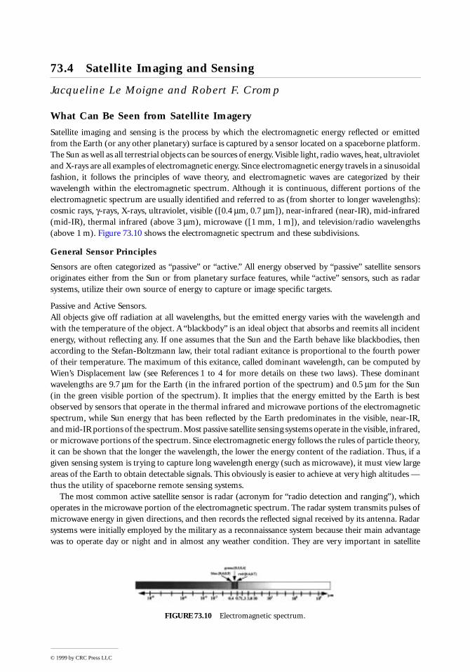
73.4 Satellite Imaging and Sensing

Jacqueline Le Moigne and Robert F. Cromp

What Can Be Seen from Satellite Imagery

Satellite imaging and sensing is the process by which the electromagnetic energy reflected or emittedfrom the Earth (or any other planetary) surface is captured by a sensor located on a spaceborne platform.The Sun as well as all terrestrial objects can be sources of energy. Visible light, radio waves, heat, ultravioletand X-rays are all examples of electromagnetic energy. Since electromagnetic energy travels in a sinusoidalfashion, it follows the principles of wave theory, and electromagnetic waves are categorized by theirwavelength within the electromagnetic spectrum. Although it is continuous, different portions of theelectromagnetic spectrum are usually identified and referred to as (from shorter to longer wavelengths):cosmic rays, g-rays, X-rays, ultraviolet, visible ([0.4 mm, 0.7 mm]), near-infrared (near-IR), mid-infrared(mid-IR), thermal infrared (above 3 mm), microwave ([1 mm, 1 m]), and television/radio wavelengths(above 1 m). Figure 73.10 shows the electromagnetic spectrum and these subdivisions.

General Sensor Principles

Sensors are often categorized as “passive” or “active.” All energy observed by “passive” satellite sensorsoriginates either from the Sun or from planetary surface features, while “active” sensors, such as radarsystems, utilize their own source of energy to capture or image specific targets.

Passive and Active Sensors.All objects give off radiation at all wavelengths, but the emitted energy varies with the wavelength andwith the temperature of the object. A “blackbody” is an ideal object that absorbs and reemits all incidentenergy, without reflecting any. If one assumes that the Sun and the Earth behave like blackbodies, thenaccording to the Stefan-Boltzmann law, their total radiant exitance is proportional to the fourth powerof their temperature. The maximum of this exitance, called dominant wavelength, can be computed byWien’s Displacement law (see References 1 to 4 for more details on these two laws). These dominantwavelengths are 9.7 mm for the Earth (in the infrared portion of the spectrum) and 0.5 mm for the Sun(in the green visible portion of the spectrum). It implies that the energy emitted by the Earth is bestobserved by sensors that operate in the thermal infrared and microwave portions of the electromagneticspectrum, while Sun energy that has been reflected by the Earth predominates in the visible, near-IR,and mid-IR portions of the spectrum. Most passive satellite sensing systems operate in the visible, infrared,or microwave portions of the spectrum. Since electromagnetic energy follows the rules of particle theory,it can be shown that the longer the wavelength, the lower the energy content of the radiation. Thus, if agiven sensing system is trying to capture long wavelength energy (such as microwave), it must view largeareas of the Earth to obtain detectable signals. This obviously is easier to achieve at very high altitudes —thus the utility of spaceborne remote sensing systems.

The most common active satellite sensor is radar (acronym for “radio detection and ranging”), whichoperates in the microwave portion of the electromagnetic spectrum. The radar system transmits pulses ofmicrowave energy in given directions, and then records the reflected signal received by its antenna. Radarsystems were initially employed by the military as a reconnaissance system because their main advantagewas to operate day or night and in almost any weather condition. They are very important in satellite

FIGURE 73.10 Electromagnetic spectrum.


remote sensing because microwave radiations are hardly affected by atmospheric “screens” such as lightrain, clouds, and smoke. The time it takes for the radar signal to return to the satellite is also measuredby instruments such as altimeters which are very useful in determining surface height measurements.

Polar Orbiting and Geostationary Earth Sensing Satellites.Satellite remote sensing systems are also characterized by the different Earth orbiting trajectories of agiven spacecraft. These two modes are usually referred as “polar orbiting” and “geostationary” (or“geosynchronous”) satellites. A polar orbit passes near the Earth’s North and South poles. Landsat, SPOT,and NOAA are near-polar satellites; their orbits are almost polar, passing above the two poles and crossingthe equator at a small angle from normal (e.g., 8.2° for Landsat-4 and -5). If the orbital period of a polarorbiting satellite keeps pace with the Sun’s westward progression compared to the Earth rotation, thesesatellites are also called “sun-synchronous.” This implies that a sun-synchronous satellite always crossesthe equator at the same local sun time. This time is usually very carefully chosen, depending on theapplication of the sensing system and the type of features that will be observed with such a system. It isoften a tradeoff between several Earth science disciplines such as atmospheric and land science. Atmo-spheric scientists prefer observations later in the morning to allow for cloud formation, whereas theresearchers performing land studies prefer earlier morning observations to minimize cloud cover.

A geostationary satellite has the same angular velocity as the Earth so its relative position is fixed withrespect to the Earth. Examples of geostationary satellites are the GOES (“Geostationary OperationalEnvironmental Satellite”) series of satellites that orbit at a constant relative position above the equator.

Sensor Characteristics

Spectral Response Patterns.The design of new satellite instruments is based on the principle that targets of interest can be identifiedbased on their spectral characteristics. For example, different Earth surface features, such as vegetationor water, present very distinctive reflectance or emittance curves that are a function of the energywavelength. These curves are often called the “spectral signatures” of the objects being observed. Althoughthese curves are very representative of each feature and can help identify them, they do not correspondto unique and absolute responses. Because of different reasons, such as atmospheric interactions, temporalor location variations, the response curves of a given object observed under different conditions mightvary. For this reason, these curves are often called “spectral response patterns” instead of “spectralsignatures.” Figure 73.11 shows an example of such reflectance patterns for several features: fir tree, clearlake water, barley, and granite.

Atmospheric Interactions.Earth satellite sensors are designed to take into consideration the fact that all observed radiation mustpass at least once through the atmosphere; therefore, the energy interactions of the atmosphere must beconsidered during the design phase. The distance through which the radiation passes through theatmosphere is called “path length.” The effect of the atmosphere depends on the extent of the path lengthand on the magnitude of the energy signal. The two main atmospheric effects are known as “scattering”and “absorption.”

Scattering is the unpredictable redirection of radiation by particles suspended in the atmosphere. Thetype and the amount of scattering mainly depend on the size of the particles but also on the wavelengthof the radiation and the atmospheric path length. If these particles are smaller than the radiationwavelength, this effect is known as “Rayleigh scatter.” This scattering especially affects the shorter visiblewavelengths of the sunlight (i.e., blue visible wavelength) and it explains why the sky appears blue to thehuman eye. In the evening, when the path length is longer, the effect of the Rayleigh scatter is only visibleon the longer red wavelengths of the sunlight and the sky appears red or orange. If the particles are aboutthe size of the radiation wavelength, the scatter is known as “Mie scatter”; this scattering effect is oftendue to water vapor and dust. When the atmospheric particles are larger than the radiation wavelengths,a “nonselective scatter” occurs; all visible wavelengths radiations are scattered equally and this type ofscattering explains why clouds appear white.


Atmospheric absorption occurs in specific wavelengths at which gases such as water vapor, carbondioxide, and ozone absorb the energy of solar radiations instead of transmitting it. “Atmospheric win-dows” are defined as the intervals of the electromagnetic spectrum outside these wavelengths, and Earthremote sensors usually concentrate their observations within the atmospheric windows. As an example,white areas of Figure 73.11 show the portions of the spectrum (i.e., the “channels” or “bands”) fromvisible to mid-IR used by the Landsat-Thematic Mapper (TM).

Spectral, Radiometric, Spatial, and Temporal Resolutions.Although the spectral response patterns are not absolute, they play an important role in the design ofnew sensors. When a new sensor is being designed, the type of features to observe and the accuracy withwhich they will be mapped define which wavelengths are of interest, the widths of the wavelength intervalsto be used, what is the accuracy to be achieved in these bandwidths, and what is the “smallest” or “faintest”feature that might be detected by the sensor. Following the examples of Figure 73.11, the best wavelengthinterval to distinguish between vegetation and granite will be the [1.55 mm, 1.75 mm] wavelength interval.The above sensor requirements correspond to the “resolutions” of the sensor by which it is usuallyidentified — spectral, radiometric, spatial, and temporal resolutions. The term “resolution” is usuallyemployed to define the smallest unit of measurement or granularity that can be recorded in the observeddata. The spectral resolution of a sensor is defined by the bandwidths utilized in the electromagneticspectrum. The radiometric resolution defines the number of “bits” that are used to record a given energycorresponding to a given wavelength. The spatial resolution corresponds to the area covered on the Earth’ssurface to compute one measurement (or one picture element, “pixel”) of the sensor. The temporalresolution (or frequency of observation), defined by the orbit of the satellite and the scanning of thesensor, describes how often a given Earth location is covered by the sensor.

FIGURE 73.11 Examples of spectral response patterns for four different types of features, fir tree, clear water, barley(example of crop), and granite (example of rock). White areas show the portions of the spectrum corresponding tothe 7 channels of Landsat-Thematic Mapper (TM-4&5).


Signal-to-Noise Ratio.Sensors are also characterized by their signal-to-noise ratio (SNR) (i.e., the noise level relative to thestrength of the signal). In this case, the “noise” usually refers to variations of intensity that are detectedby the sensor and that are not caused by actual variations in feature brightness. If the noise level is veryhigh compared to the signal level, the data will not provide an accurate representation of the observedfeatures. At a given wavelength l , SNR is a function of the detector quality, the spatial resolution of thesensor, as well as its spectral resolution (see Reference 1 for a detailed formula). To maintain or improvethe signal-to-noise ratio and therefore improve the radiometric resolution of the sensor, a tradeoff mustbe made between spatial and spectral resolutions; in particular, improving spatial resolution will decreasethe spectral resolution. Of course, other factors such as atmospheric interactions will also affect the SNR.

Multispectral and Hyperspectral Sensors.The remote sensing industry is experiencing a rapid increase in the number of spectral bands of eachsensor. The first Landsat sensors (Landsat-1 and 2) were designed with four bands in the visible andnear-IR portions of the spectrum. Landsat-4 and 5 were refined with seven bands from visible to thermal-IR. Then, Landsat-6 and 7 were planned with an additional panchromatic band, which is highly sensitiveover the visible part of the spectrum. In general, most Earth remote sensors are multispectral; that is,they utilize several bands to capture the energy emitted or reflected from Earth features. The additionof panchromatic imagery, which usually has a much better spatial resolution than multispectral imageryin the visible part of the spectrum, provides higher quality detail information. Multispectral and pan-chromatic data, usually acquired simultaneously, are co-registered and can be easily merged to obtainhigh spatial and spectral resolution. Co-registered multispectral-panchromatic imagery is available fromsensors such as the Indian satellite sensor, IRS-1, and the French sensor, SPOT.

Ideally, if a sensor had an infinite number of spectral channels (or bands), each observed area on theground (or pixel) could be represented by a continuous spectrum and then identified from a databaseof known spectral response patterns. Adding more bands and making each of them narrower is the firststep toward this ideal sensor. But, as previously explained in the previous section, due to technologylimitations, it was very difficult until recently to increase the number of bands without decreasing theSNR. Due to recent advances in solid state detector technology, it is now possible to increase significantlythe number of bands without decreasing the SNR, thus seeing the rise of new types of sensors, calledhyperspectral. Although the boundary between multispectral and hyperspectral sensors is sometimesdefined as low as 10 bands, hyperspectral imaging usually refers to the simultaneous detection in hundredsto thousands of spectral channels. The aim of hyperspectral sensors is to provide unique identification(or “spectral fingerprints”) capabilities for resolvable spectral objects. Potential applications includeagricultural yield monitoring, urban planning, land use mapping, mining and mineral deposits, disasterrelief/assessment, tactical military operations, and forest fire protection management. The NASA Air-borne Visible InfraRed Imaging Spectrometer (AVIRIS) simultaneously collects spectral information fromvisible to infrared ranges (from 0.4 mm to 2.5 mm) in 224 contiguous spectral bands. Each band has anapproximate bandwidth of 10 nm (or 0.01 mm), with a spatial resolution of about 20 m. The instrumentflies aboard a NASA ER-2 airplane at approximately 20 km above sea level. The science objectives of theAVIRIS project are mainly directed toward understanding processes related to the global environmentand climate change.

Super-Resolution.When data is collected from a satellite sensor, each sample of information represents an area on theground that might correspond to several features with different spectral responses and the final infor-mation represents a “mixture” of several disparate information. When a sensor does periodic imagingover the same area, the direction of observation slightly changes, and even when successive data arecorrectly registered (i.e., in a perfect correspondence), two respective samples might represent two slightlydifferent areas on the ground. Super-resolution is an area of research that aims at combining such


information from different directions but taken under similar lighting conditions in the goal of improvingspatial and spectral resolutions. As an example, some recent work [5] utilizes a Bayesian method forgenerating sub-pixel resolution composites from multiple images with different alignments. Softwareproducts have also been proposed by some commercial systems, such as ERDAS-Imagine and ENVI, tohelp in the unmixing of spectral bands (see Reference 6 for more detail).

Direct Readout Data

Examples of different spectral and spatial resolutions are given in Table 73.9 with a summary of currentEarth remote sensing systems that operate from visible to thermal-IR wavelengths. Table 73.9 providesinformation about their bandwidths and their spatial resolutions. The table also indicates if the datafrom these sensors can be acquired by direct readout. Sensors can transmit data in two modes. The firstmode, called “direct readout,” transmits data as soon as it “sees” it, and any receiving station within thatsatellite footprint can receive this data. In the second mode, the sensor records whatever it sees forplayback at a later time, and specialized receiving stations (or “ground stations”) are required to receivethis data since it is transmitted at higher rates than direct readout. The data received by these groundstations can cover a larger extent. Historically, the cost of acquiring and processing Earth remotely senseddata has limited satellite data collection to a small number of expensive ground stations around theworld, operated by the owners of the satellites. Direct readout sensors were mostly confined to meteo-rological applications that required timely data such as weather forecasting, severe weather identificationand tracking, and disaster prediction and assessment. But this situation is changing; due to new tech-nology, costs have been greatly reduced, and direct readout data that was initially expensive and beyondthe reach of the nontraditional user, is now generating a growing interest. A small industry has evolvedto design, install, and upgrade ground stations around the world that acquire direct readout data.

Typical Attributes Measured from Space

This section does not intend to be an exhaustive up-to-date description of all Earth and space applicationsof satellite imaging and sensing, but rather it presents a few representative applications and their associatedsatellite sensors. The References section as well as the World Wide Web (WWW) offer more extensivereferences to other applications and sensors.

Earth Science Applications.Over the past few decades, a number of international global change research programs have been initiatedwhose goals are to understand the relation between human activities and the global Earth systemsprocesses and trends. Mission To Planet Earth (MTPE [7]) is a multi-agency program, whose goal is toachieve this kind of understanding, especially through improved satellite observations. As part of NASA’sMission to Planet Earth program, the Earth Observing System (EOS [8]) will launch, over the next2 decades, several platforms of sensors aimed at ecology, oceanography, geology, snow, ice, hydrology,cloud, and atmospheric studies. Each platform will carry one or several instruments, thus globallycovering a wide range of spectral, spatial, and temporal resolutions. Europe and Japan have similarprograms, such as the ADEOS (ADvanced Earth Observation Satellite [9]), developed by the Japanesespace agency, NASDA, in collaboration with France and the U.S. ADEOS, launched in 1996, flew for9 months before it failed, and included remote sensing instruments for observing the Earth’s atmosphere,land surfaces, and oceans. Other examples of such programs are the ERS and ENVISAT satellites fromESA (European Space Agency) and the Indian satellites, IRS. ERS-1 and 2 were launched in 1991 and1995, respectively, and ENVISAT will be launched in 1999. All these satellites carry on the same platformdifferent instruments making simultaneous observations. The first satellite in the IRS series was launchedin 1988, and in 9 years, India has designed and launched six remote sensing satellites. For more infor-mation on the IRS series, see Reference 10.

In all the above programs, studies concentrate on global processes occurring in the atmosphere(especially lower parts of the atmosphere), on the Earth surface (terrestrial studies), and in the oceans(hydrospheric studies). Results of all these studies will contribute to international programs such as the


TAB

LE 7

3.9

Sum

mar

y of

th

e M

ain

Cu

rren

t E

arth

Sci

ence

Sat

ellit

e D

ata

Ope

rati

ng

from

UV

to

Th

erm

al I

R (

“D”:

Dir

ect

Bro

adca

st)


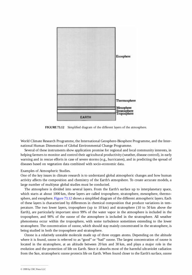
World Climate Research Programme, the International Geosphere-Biosphere Programme, and the Inter-national Human Dimensions of Global Environmental Change Programme.

Several of these instruments show application promise for regional and local community interests, inhelping farmers to monitor and control their agricultural productivity (weather, disease control), in earlywarning and in rescue efforts in case of severe storms (e.g., hurricanes), and in predicting the spread ofdiseases based on vegetation data combined with socio-economic data.

Examples of Atmospheric Studies.One of the key issues in climate research is to understand global atmospheric changes and how humanactivity affects the composition and chemistry of the Earth’s atmopshere. To create accurate models, alarge number of multiyear global studies must be conducted.

The atmosphere is divided into several layers. From the Earth’s surface up to interplanetary space,which starts at about 1000 km, these layers are called troposphere, stratosphere, mesosphere, thermo-sphere, and exosphere. Figure 73.12 shows a simplified diagram of the different atmospheric layers. Eachof these layers is characterized by differences in chemical composition that produce variations in tem-perature. The two lower layers, troposphere (up to 10 km) and stratosphere (10 to 50 km above theEarth), are particularly important since 99% of the water vapor in the atmosphere is included in thetroposphere, and 90% of the ozone of the atmosphere is included in the stratosphere. All weatherphenomena occur within the troposphere, with some turbulence sometimes extending to the lowerstratosphere. The concentration of ozone, which should stay mainly concentrated in the stratosphere, isbeing studied in both the troposphere and stratosphere.

Ozone is a relatively unstable molecule made up of three oxygen atoms. Depending on the altitudewhere it is found, ozone is referred to as “good” or “bad” ozone. The largest concentration of ozone islocated in the stratosphere, at an altitude between 20 km and 30 km, and plays a major role in theevolution and the protection of life on Earth. Since it absorbs most of the harmful ultraviolet radiationfrom the Sun, stratospheric ozone protects life on Earth. When found closer to the Earth’s surface, ozone

FIGURE 73.12 Simplified diagram of the different layers of the atmosphere.


may be harmful to lung tissue and plants. Recent studies have shown that the proportions of ozone inthe air are increasing compared to decreasing amounts of protective ozone. However, studies still needto determine if these changes are due to human activity or if they are part of regular natural cycles.

The mission of the Total Ozone Mapping Spectrometer (TOMS) is to provide global measurementsof total column ozone as well as of sulfur dioxide on a daily basis. The TOMS instrument measures thereflectivity of the atmosphere in six near-UV wavelengths (see Table 73.9) and provides differential UVabsorption and surface reflectivity data. From these measurements, total ozone is computed by searchingprecomputed albedo tables, which depend on solar zenith angle, view angle, latitude, surface reflectance,and surface pressure; a lower amount of radiation measured by TOMS corresponds to higher concen-trations of ozone. Maps of volcanic eruptions are a byproduct of TOMS sulfur dioxide measurements.The first TOMS instrument was flown on Nimbus 7 in 1978; successive ones were launched on a RussianMeteor spacecraft in 1991, on an Earth Probe satellite in 1994, and on the Japanese ADEOS satellite in1996. See References 11 to 16 for more information on TOMS and ozone measurements.

The TOMS measurements are also being compared to the ozone measurements provided by the NOAA(National Oceanic and Atmospheric Administration) series of the Television Infrared Observing Satellite(TIROS) Operational Vertical Sounder (TOVS) data. The TOVS sounding unit consists of three instru-ments, including the High-Resolution Infrared Sounder-2 (HIRS-2) whose channels are shown inTable 73.9. TOVS-type instruments have been flying since 1978. These instruments provide informationabout the structure of the atmosphere, vertical temperature and moisture profiles, as well as cloudamounts and heights. Through analysis of this data, the TOVS Pathfinder data set is created and contains74 layers of measurements on attributes such as temperature, water vapor, ozone level, precipitation,cloud coverage, etc. taken at various atmospheric pressure levels (e.g., 1000 mb, 850 mb, etc.). A fullglobal coverage of TOVS data is produced twice daily, and a 16-year global data set for climate studiesis being gathered [17].

Another satellite that obtains atmospheric data is the Upper Atmosphere Research Satellite (UARS).UARS was launched in 1991 and performs a comprehensive study of the stratosphere and furnishesimportant new data on the mesosphere and the thermosphere. UARS operates 585 km above the Earthin a near circular orbit inclined 57° to the equator. This orbit permits UARS sensors to provide globalcoverage of the stratosphere and mesosphere and measurements are made approximately every 36 days.The ten UARS chemistry and dynamics sensors are making measurements of temperature, pressure, windvelocity, and gas species concentrations. All these simultaneous measurements will help define the roleof the upper atmosphere in our climate and its variability.

The Tropical Rainfall Measuring Mission (TRMM, [18]) is a joint project between the United Statesand Japan. The goal of this project is to measure precipitation at tropical latitudes and to provide accuratemapping of tropical rainfall. The mission consists of three instruments: a precipitation radar, a multi-channel microwave radiometer, and a visible-infrared scanner. The data provided by TRMM will be veryimportant to verify and develop climate models.

The French space agency, CNES, has also developed the POLDER (POLarization and Directionalityof the Earth’s Reflectances) instrument, which flew on ADEOS. This is the first French/Japanese coop-erative project in the area of Earth observation. A second, identical instrument is to be flown on ADEOS-2,successor to ADEOS, in 1999. POLDER is a wide field-of-view imaging radiometer that will provideglobal, systematic measurements of spectral, directional, and polarized characteristics of the solar radi-ation reflected by the Earth/atmosphere system, as well as aerosols, land and sea surfaces, and water vapormeasurements.

NOAA’s AVHRR (Advanced Very High Resolution Radiometer [19]) is very useful to study biomassburning in the tropics, and the interactions of smoke particles with clouds. More generally, informationfrom the five AVHRR channels (see Table 73.9) is integrated into clouds and climate models.

Weather images are an everyday occurance televised all over the world. Several weather satellites areoperated by several countries. In the U.S., NASA and NOAA are operating the GOES series of geosta-tionary satellites, which provide global weather data every 30 min since 1974, positioned at 36,000 km


above the Earth. GOES image and sounder data are also used for climate studies. In Europe, the Meteosatweather satellites are developed and launched by ESA, and financed and owned by Eumetsat, an inter-national organization of 17 European weather services. Meteosat-1 was launched in 1977, followed byfive others in 1981, 1989, 1991, and 1993. Three of them are currently in service, each equipped with animaging radiometer. Table 73.9 shows the spectral ranges of operations of these two series of geostationarysatellites. Several channels in the visible, water vapor, and thermal-IR spectral bands provide importantinformation about cloud coverage, storm formation and evolution, as well as Earth radiation.

Examples of Terrestrial Studies.Land Cover Applications. There are two basic types of data considered most important for global changeresearch [20]; the data for documenting and monitoring global change, and the data for discovering thedynamical interplay among the various elements that define our environment. Previous studies showthat global studies of land transformations require extrapolation among several scales (spatial, radiomet-ric, and temporal). This extrapolation is especially important to control the minimum detectable change,whether spatial, spectral, or temporal. This accuracy in change detection, which is based on the propertiesof the sensing systems [21], can be especially essential in distinguishing between nature- and human-induced changes.

Getting accurate quantitative information about the distribution and the areal extent of the Earth’svegetation formations is a basic requirement in understanding the dynamics of the major ecosystems.Among all land transformations most critical to study for global change research, the assessment oftropical forests is one of the most important [22-25]. The tropical forest biome forms 7% of the Earthland surface, and its extensive loss could have a major impact on the future of the Earth (habitatfragmentation, species extinction, soil degradation, global climatic modifications, etc.). Previous studieshave shown that in the last 2 decades, 50% of the areal extent of tropical forests might have been lost todeforestation [23]. At present, there is a wide range of estimates of the areal extent of tropical forests andof their rates of deforestation. Therefore, there is a great need to produce accurate and up-to-datemeasurements concerning the Tropical Forest worldwide. A range of different sensors must be utilizedfor such applications.

Other examples of land cover applications include agriculture and crop forecasting, water urbanplanning, rangeland monitoring, mineral and oil exploration, cartography, flood monitoring, diseasecontrol, real estate tax monitoring, detection of illegal crops, etc. In many of these applications, thecombination of remote sensing data and Geographic Information Systems (GISs; see References 26 and27) show great promise in helping the decision-making process.

Most instruments utilized to observe land features are on-board low Earth orbit satellites and aremultispectral sensors with two or three bands in the visible part of the spectrum and at least one bandin the infrared [6].

The Landsat series of satellites is the oldest land monitoring satellite system. Initiated in 1967, theEarth Resource Technology Satellites (ERTS) program was planning a series of six satellites to performa broad-scale, repetitive survey of the Earth’s land areas. After the launch in 1972 of the first ERTS-1, theERTS program was renamed “Landsat.” As of 1997, five Landsat satellites have been launched, each onecarrying two instruments. The payload of Landsat-1 and -2 included a Return Beam Vidicon (RBV)camera and a Multispectral Scanner (MSS), while Landsat-4 and -5 still use the MSS and the ThematicMapper (TM). The first RBV system consisted of three television-like cameras with a ground resolutionof 80 m, each looking respectively at the green, red, and near-infrared portions of the spectrum. OnLandsat-3, the RBV was 30 m panchromatic. MSS quickly became of primary interest due mainly to itscapability of producing multispectral data in a digital format. The four MSS spectral bands are shownin Table 73.9, and the spatial resolution of MSS data is about 80 m. Very early on, the utility of MSS datawas recognized for such applications as agriculture, mapping, forest monitoring, geology, as well as waterresource analysis. The same MSS system was kept on Landsat-4 and -5, but the RBV system was replacedby the TM system. Like MSS, TM is a multispectral scanner, but includes spatial, spectral, and radiometricimprovements over MSS. With seven bands instead of four (see Table 73.9), TM covers a larger portion


of the visible wavelengths, and includes two mid-IR and one thermal-IR bands. Data are quantized over256 levels (8 bits) instead of the 64 levels for MSS, and the spatial resolution of a TM pixel is about 30 m.TM data is usually chosen to perform classification of land-cover features, man-made or natural. Invegetation and change detection applications, leaf segmentation is studied with TM visible channel data,while cell structure can be seen in near-IR, and leaf water content is found in the mid-IR channel data.The two mid-IR bands (5 and 7) are also useful for geologic applications. All the Landsat satellites areplaced in low Earth orbit (at an altitude of about 900 km for Landsat-1 to -3 and 705 km for Landsat-4and -5) and in a near-polar, sun-synchronous orbit. Landsat-4 and -5 cross the equator at 9:45 a.m. tohopefully take advantage of cloud-free imagery. Landsat-4 and -5 have a 16-day repeat cycle and theirorbits are 8 days out of phase. Landsat-6 failed to achieve orbit in 1993; Landsat-7 is planned to belaunched in 1998 and includes an improved TM instrument, the Enhanced Thematic Mapper (ETM),which will also include a panchromatic band at a spatial resolution of 15 m. For a more in-depthdescription of Landsat systems, see References 1, 29, and 30; for more applications and analysis of Landsatdata, see Reference 30.

As previously mentioned, NOAA’s AVHRR is primarily used for atmospheric applications but is alsoutilized for land surface applications. Having a near-polar, sun-synchronous orbit (at 833 km above theEarth’s surface), the AVHRR instrument provides global data with a 1.1-km spatial resolution at nadir,and includes five bands, with daily or twice-daily (for thermal-IR) coverage. Since 1978, AVHRR dataare available at full resolution (called Local Area Coverage (LAC)) or subsampled to 4 km (known asGlobal Area Coverage (GAC)). Because of its high temporal resolution, the AVHRR instrument is veryuseful in applications such as flood, storm, or fire monitoring, as well as volcanic eruption. Because ofits global area coverage, AVHRR is also often utilized for studying geologic or physiographic features,vegetation conditions and trends at a global, continental or regional level, snow cover mapping, soilmoisture analysis, and sand storms and volcanic eruptions worldwide. A popular parameter extractedfrom AVHRR data is the Normalized Difference Vegetation Index (NDVI), computed from GAC data as:NDVI = (Channel 2 – Channel 1)/(Channel 1 + Channel 2). GAC data is processed daily and compositedon a weekly basis to produce a global map showing vegetation vigor. An example of NDVI applicationsis the monitoring of the Sahara desert extent. AVHRR data are also used for sea surface temperature.

The first Système Pour l’Observation de la Terre (SPOT), designed by CNES, was launched in 1986.SPOT-2 and SPOT-3 were launched, respectively, in 1990 and 1993. The SPOT satellites fly in a near-polar, sun-synchronous low Earth orbit at an altitude of 832 km and cross the equator at 10:30 a.m.SPOT’s repeat cycle is 26 days, but due to its off-nadir viewing capability (viewing angle up to 27°), SPOThas a “revisiting” capability with which the same area can be seen up to five times every 26 days. Thisoff-nadir viewing capability also enables some stereo imaging possibilities. The SPOT payload includestwo identical high-resolution-visible (HRV) imaging instruments that can be employed in panchromaticor multispectral modes, with pointing capabilities. Spectral coverage of these two modes is given inTable 73.9. The panchromatic mode is 10 m spatial resolution, while multispectral data have a 20 mspatial resolution. Whereas Landsat is a scanning mirror-type instrument, SPOT employs a push-broomsystem with a linear array of detectors simultaneously acquiring all data pixels in one image line, whichminimizes geometric errors. SPOT data are very useful for applications involving small features. Due toits increased spatial resolution, revisit and pointing capabilities, simultaneous panchromatic and multi-spectral data, and stereo data capabilities, SPOT opens a new range of applications, such as topographicmapping, studies of earthflows (e.g., land, rock, and mudslides), urban management, and militaryapplications. SPOT-4 is planned for launch in 1998, and SPOT-5 in 2002. Among the planned improve-ments, a mid-IR channel will be added to SPOT-4, which will also carry a new AVHRR-type instrument,the European Vegetation instrument.

Since 1988, India has launched a series of five satellites, the IRS series. These satellites were designedin support of India’s agriculture and exploration businesses, and they seem to be successful in thischallenge of bringing remote sensing to the users (see Reference 10). For land applications, IRS-1A, -1B,and -1C all carry the LISS instrument, which is a multispectral scanner very similar to Landsat-TM.LISS-2 acquires imagery in four bands similar to bands 1 to 4 of Landsat-TM (from visible to near-IR)


at the spatial resolution of 36.5m (see Table 73.9 for wavelengths description). LISS-3, carried on IRS-1C,also acquires imagery in four bands, but the visible blue band has been suppressed and replaced by amid-IR band similar to TM/band 5. Due to their similarity to Landsat data, IRS/LISS-2 data could beused as complements or replacements to Landsat data if needed until Landsat-7 is launched. IRS-1C alsocarries a 5-m panchromatic imstrument whose data are co-registered with LISS-2 data. For more detailson IRS data, see References 10 or 27.

Other instruments are also available. JERS-1, designed by Japan, was launched in 1992, and its payloadincludes both an SAR instrument and an optical-imaging system; see Table 73.9 for its spectral channelsfrom visible to mid-IR wavelengths, with spatial resolutions of 18 m and 24 m. MOMS, the GermanModular Optoelectronic Multispectral Scanner, has been flying as a research instrument on U.S. SpaceShuttle missions, and has a spatial resolution ranging from 4.5 m to 13.5 m; see Reference 27 for moredetails on these different instruments.

Among the first EOS intruments to be launched is the Moderate Resolution Imaging Spectrometer(MODIS). MODIS is being developed to provide global monitoring of the atmosphere, terrestrial eco-system, and oceans, and to detect climate change. MODIS will cover the visible to infrared portions ofthe spectrum with 36 channels at spatial resolutions of 250 m to 1 km. Many interesting land studies willbe performed by fusing together AVHRR, Landsat, and MODIS data.

The fusion of several of these types of data is becoming a very important issue [26]. Already, sensorssuch as SPOT or LISS-3 present the advantage of acquiring co-registered panchromatic and multispectraldata. It would be of great interest to combine data from sensors with different spectral and spatialresolutions, as well as different viewpoints. The combination of coarse-resolution viewing satellites forlarge area surveys and finer resolution sensors for more detailed studies would offer the multilevelinformation necessary to assess accurately the areal extent of features of interest (e.g., tropical forests).The fusion of multispectral data with SAR data would provide information on ground cover reflectancewith the shape, roughness, and moisture content information from SAR. Of course, multidata fusionrequires very accurate registration of the data, as will be described in Section 2.4.

Geologic Studies. Other examples of terrestrial studies are the mapping of geologic features, such asgeologic faults and earthquake sites, or volcanic eruptions. Although many geologic features lie beneaththe surface of the Earth, remote sensing (aerial or satellite) provides a valuable tool to perform geologicmapping, landforms and structures analysis, as well as mineral exploration. This is due to the fact thattopography and soil properties provide clues to underlying rocks and structural deformations. Landsatand SPOT gather data about the effects of subsurface geologic phenomena on the surface. These dataare especially useful to recognize some specific landforms (such as volcanoes), to depict topographicfeatures, discriminate some geologic facies and rock unit distribution patterns and more generally provideregional overviews of surface geology. In mineral exploration, rock or soil alteration can be detected byspaceborne sensors and may indicate the presence of mineral deposits or oil reservoirs. Other types ofsensors that are very useful for geologic applications are radar sensors, such as the two radar systems,SIR-C and X-SAR, carried on the Space Shuttle Endevour in 1994. These sensors captured in real-timethe eruption of a volcano in Russia and an earthquake in Japan [31]. For more information on geologicapplications, see References 2 and 32.

Geophysics Studies. Other satellites, such as the LAEGOS-1 and -2, have proved very useful in geo-physics for the study of the Earth’s gravity field, tectonic plate motion, polar motion, and tides. LAGEOSsensors are reflector orbs covered with laser beams. For more information on these studies, seeReferences 33 and 34.

Examples of Ocean Studies.Oceans cover 75% of the Earth’s surface and contain most of the energy of the planet. Although their rolein climate evolution is very important, it is still poorly understood. By understanding chemical, physical,and biological processes in oceans, scientists will be able to model the interactions between oceans andthe atmosphere and determine how these interactions affect Earth temperature, weather, and climate.


An example of interaction between oceans and the atmosphere is illustrated by the phenomenonknown as El Niño/Southern Oscillation, which occurs in the tropical Pacific Ocean, usually aroundChristmas time. El Niño is due to a mass of warm water, usually located off Australia which moveseastward toward equatorial South America. El Niño develops every few years (observed on average every4 years to a maximum of 7 years), and alters the weather in Australia, Africa, South Asia, and the tropicalparts of the Americas. By understanding how winds and waves move in the tropical Pacific, scientistshave been able to predict the El Niño phenomenon up to 1 year in advance. Similar phenomena are beingstudied in the Atlantic Ocean, where patterns seem to move much more slowly.

Besides being used to create global models, and in storm and weather forecasting, ocean data are alsovery important for day-to-day applications such as ship routing, oil production, and ocean fishing.

Ocean Color. Ocean color data are critical for the study of global biogeochemistry and to determinethe ocean’s role in the global carbon cycle and the exchange of other critical elements and gases betweenthe atmosphere and the ocean [35,36]. It is thought that marine plants remove carbon from the atmo-sphere at a rate equivalent to terrestrial plants, but knowledge of interannual variability is very poor. Formost oceans, the color observed by satellite in the visible part of the spectrum varies with the concen-tration of chlorophyll and other plant pigments present in the water. Subtle changes in ocean color usuallyindicate that various types and quantities of microscopic marine plants (i.e., phytoplankton are presentin the water); the more phytoplankton present, the greater the concentration of plant pigments and thegreener the water.

The recently launched (October 1997) Sea-viewing Wide Field-of-view Sensor (SeaWiFS,), which is apart of MTPE, provides quantitative data on global ocean bio-optical properties to the earth sciencecommunity. SeaWiFS is a follow-on sensor to the Coastal Zone Color Scanner (CZCS), which ceasedoperations in 1986. See Table 73.9 for a channel description of these two sensors; notice that all channelsare concentrated in the [0.4,0.7] interval of the electromagnetic spectrum.

Other sensors for ocean color are the imaging spectrometer for ocean color applications MOS-IRS,launched on the Indian Remote Sensing Satellite IRS-P3 in March 1996, and the imaging spectrometerMOS-PRIRODA, launched aboard the Russian multisensor remote sensing module PRIRODA anddocked to space station MIR in April 1996.

Ocean Dynamics. By studying ocean circulation and sea levels trends, scientists will be able to createglobal maps of ocean currents and of sea surface topography. Since sea surface height and sea levelvariations are related to sea surface temperatures, the monitoring of mean sea levels enables the gatheringof evidence that can measure global warming or El Niño-type events. For example, conditions related toEl Niño may result in a change in sea surface height of 18 cm or greater [37].

TOPEX/Poseidon (T/P) is an important collaboration between U.S./NASA and France/CNES. T/P usesradar altimetry to provide 10-day maps of the height of most of the ice-free oceans’ surface. Circling theworld every 112 min, the satellite gathers data for 3 to 5 years, and could be operational for 10 years. TheT/P satellite was launched in August 1992 on an Ariane rocket. TOPEX measures the height of the oceansurface, as well as changes in global mean sea level. From these altimetry data, global maps of oceantopography are created, from which speed and direction of ocean currents are computed worldwide.Changes in mean sea level are monitored and currently are viewed mostly as related to natural oceanvariability and not climate change. Climate change must be studied over a much longer time series ofaltimeter data. T/P also enables study of tides, waves geophysics, and ocean surface winds.

Sea winds are also being studied with scatterometers such as the NASA Scatterometer (NSCAT) andthe soon to be launched EOS Scatterometer, SearWinds. These high-frequency radar instruments measurethe reflected signals from the ocean surface to detect wind speed and direction.

ERS-1 is another satellite utilized to measure ocean dynamics. ERS-1 was launched in 1991 on a sun-synchronous, near-polar low-Earth orbit at an altitude of 780 km. ERS-1 orbits the Earth in 100 minand covers the entire planet in 3 days. Its payload consists of two specialized radars and one infraredsensor. The Active Microwave instrument, consisting of a synthetic aperture radar and wind scatterometer,produces extremely detailed images of 100 km swath of the Earth’s surface, with a spatial resolution of


20 m. The radar altimeter provides accurate range to sea surface and wave heights, and the along-trackscanning radiometer constructs detailed pictures of the thermal structure of the seas and oceans fromsurface temperature measurements at an accuracy of less than 0.5°C. ERS-1 images are also utilized forland applications where the instruments need to “look through” the cloud cover.

The study of sea ice with passive and active microwave sensors is also very important and additionalreading in this topic can be found in References 14 and 38.

A Few Examples of Space Science Applications.Astronomical satellites have been developed to observe far distant objects that are usually beyond therange of ground-based instruments. They explore phenomena in the solar system, and beyond. Satelliteobservation of astronomical objects is also less sensitive to atmospheric interactions and can achievehigher accuracy than ground-based measurements. This section will give a brief description of the mostimportant space science satellites.

The first astronomical satellite to be put into synchronous orbit was the International UltravioletExplorer (IUE) laboratory. IUE was launched in 1978 under a joint program involving NASA, ESA, andthe United Kingdom. In more than 15 years of service, IUE gathered observations on more than 10,000celestial objects. A program for coordinating its observations with those of the ROSAT satellite has beencarried out under the title RIASS (Rosat-IUE All-Sky Survey). ROSAT, the Roentgen Satellite, is a jointcollaboration between Germany, the U.S., and the U.K., and was launched in 1990. It is an X-rayobservatory that carries two instruments, the X-ray telescope and the wide field camera.

The Infrared Astronomical Satellite, IRAS, is a joint project of the U.S., the U.K., and the Netherlands.The IRAS mission was intended to provide a survey of infrared point sources (from 12 to 100 mm), buthas also produced very high-quality image data. MSX (the Mid-Course Space Experiment), ISO (theInfrared Space Observatory), and SIRTF (the Space InfraRed Telescope Facility) are other examples ofrecently or soon-to-be launched sensors that provide an even finer resolution.

Hipparcos (High Precision Parallax Collecting Satellite) is an astronomy satellite launched in August 1989,with the purpose of determining the astrometric parameters of stars with unprecedented precision. After alife of 4 years, Hipparcos has produced two catalogs. The Hipparcos Catalogue provides position, parallax,and proper motion measurements with accuracy of 2 milliarcsec at 9 mag for over 120,000 stars. The TychoCatalogue is the result of somewhat less precise astrometric measurements for some 1 million stars.

COBE, the Cosmic Origin Background Explorer developed by NASA, was launched in 1989. Designedto measure the diffuse infrared and microwave radiation from the early universe, it carried three instru-ments: a Far Infrared Absolute Spectrophotometer (FIRAS), a Differential Microwave Radiometer(DMR), and a Diffuse Infrared Background Experiment (DIRBE). The first full-sky coverage was com-pleted in 1990.

The Hubble Space Telescope (HST) is one of the most well-known astronomical satellites. It was builtas a joint NASA/ESA project, and was launched in 1990 as a long-term space-based observatory. Theheart of the system is a large reflector telescope 2.4 m in diameter. All the instruments on-board the HSTuse the light gathered by the reflector telescope. Current HST instruments are the Wide/Field PlanetaryCamera 2 (WFPC2), the Space Telescope Imaging Spectrograph (STIS), the Near-Infrared and ImagingSpectrograph (NICMOS), and the Faint Object Camera, FOC, provided by ESA. These different instru-ments can observe astronomical objects from UV to IR wavelengths. In 1993, the HST was serviced tocorrect a preliminary fault affecting the mirror with a corrective optical apparatus named COSTAR.Despite the preliminary mirror fault, and even more after correction, the HST has achieved much betterresults than those from observatories on Earth. Since it is located above the Earth’s atmosphere (at 600km), the HST produces highly detailed images of the stars and can detect objects beyond the range ofground-based instruments. Observations with the HST are scheduled as a space-based observatoryaccording to worldwide astronomers’ proposals.

ASCA, the Advanced Satellite for Cosmology and Astophysics, is the product of a Japan/U.S. collab-oration. Launched in 1993, this X-ray astronomy mission was still operational in 1997, and carries fourlarge-area X-ray telescopes with arc minute resolution. ASCA data are being archived and can be searched


and retrieved online at the High Energy Astrophysics Science Archive Research Center, HEASARC. GRO(Gamma Ray Observatory), and AXAF (the Advanced X-ray Astrophysics Facility) are other examplesof space sensors which operate in this spectrum range.

Management and Interpretation of Satellite Data

Satellite sensors gather the electromagnetic energy reflected or emitted from Earth (or any other plane-tary) surface features. This energy is then converted into a digital representation that is visualized by auser and interpreted either visually or with a computer. This section summarizes some preliminary ideason how the digital representation is formed and the basic types of data processing necessary before anyfurther interpretation of the data. For more details on the processing of remote sensing data, seeReferences 39 to 42.

Fundamental Data Levels

After transmission from the satellites, raw data are usually processed, calibrated, archived, and distributedby a ground-based data system. Most of NASA satellite data products are classified in the following datalevels [7]:

• Level 0 data are the reconstructed raw instrument data at full resolution.• Level 1A data are reconstructed, time-reference raw data, with ancillary information including

radiometric and geometric coefficients.• Level 1B data are corrected Level 1A data (in sensor units).• Level 2 data are derived geophysical products from Level 1 data, at the same resolution and location;

for example, atmospheric temperature profiles, gas concentrations, or winds variables.• Level 3 data correspond to the same geophysical information as Level 2, but mapped onto a

uniform space-time grid.• Level 4 data are model output or results from analysis of lower-level data.

Image Restoration

Ideally, the scene as viewed and recorded by a sensor would be an exact rendering of the features withinthe sensor’s viewing extent, represented as a spectral curve indicating the amount of energy reflect-ing/radiating for each point in a scene for a range of given wavelengths. From an engineering standpoint,this is impossible, however, because each image is discretized into a finite number of pixels. Variabilitydefines nature, so each pixel will map into a region of the scene that contains a number of features, eachproducing its own unique spectral curve. The spectral signature recorded for a pixel is a function of thesefeatures and their relative sizes within the region covered by the pixel. The spectral response itself is alsodiscretized into a finite number of bandwidths, where each bandwidth covers a small continuous bandof the spectrum. The sensor records for each pixel the amount of energy observed for each band. Thisnumber itself, referred to as a Digital Number (DN), must be represented in a finite amount of computermemory, such as 8 bits, meaning that each band records activity as a whole number ranging from 0 to 255.

In practice, a number of events outside human control affect the quality of the observation, such asatmospheric scattering, variations in sun angle, high albedo, and instrument errors. Depending on theapplication, it may be desirable to correct for the presence of thin clouds within an image. The processof image restoration attempts to control and correct for these conditions [42].

Electromechanical effects due to the instrument itself can be discovered due to their periodic nature(such as caused by the repeated motion of a push-broom, or the revolving of a mirror, or the physicalprocess of gathering calibration points). A Fourier transform applied to an image from a sensor under-going periodic interference exhibits strong noise spikes. A filter can then be used to remove the offendingdata. Unfortunately, this also removes any good data that happens to fall at the same frequency, althoughnormally this is but a small portion of the data. Data outages and instrument recorder failures appearas streaks in the image parallel with the scanline, and can be discovered by comparing the respectivereadings of the pixels in the surrounding scanlines of the image.


To account for the atmospheric effects of Rayleigh and aerosol scattering, an estimate of the portionof the signal that is due to the atmosphere is computed and subtracted from the recorded value. Thereflectance of water in the near-infrared region of the spectrum should be effectively zero, so the valueto subtract for the near-IR band corresponds to the reading of the sensor observed over clear open water.To compute values to be subtracted for each of the other spectral components, a histogram should beformed for each band of a number of sample readings over clear open water. The lowest reading in eachband is then used as an estimate of the value to subtract from each pixel to account for the atmosphericeffect. In addition, information derived from TOVS, balloon readings, or the atmospheric correctionsoftware 5S can be useful in dealing with atmospheric effects.

Data Compression

Data compression is one of the most important tools to overcome the problems of data transmission,storage, and dissemination [43]. Data compression methods are usually classified as either lossless orlossy. With a lossless data compression scheme, the original data can be reconstructed exactly withoutany loss; in a lossy compression scheme, original data are reconstructed with a degree of error. Fortransmission from the satellite to the ground station, a lossless data compression must be utilized. Forbrowsing purposes, lossy compression enables quick searches through large amounts of data. A com-pression scheme is also characterized by its compression ratio, that is, the factor by which the amountof information which represents the data is reduced through compression. For earth science data, losslesscompression schemes provide compression ratios up to 2 or 3, while lossy techniques can reduce theamount of information by a factor of 20 or more without degrading the visual quality of the data.

Among the lossless compression methods, the Joint Photographic Experts Group, JPEG, developed alossless compression method that is based on a predictor, an entropy encoder for prediction error, andan entropy code specifier. Another lossless compression scheme is the Rice algorithm, which can adaptto data of any entropy range. It is based on a preprocessor that spatially decorrelates the data, followedby a variable length encoder. This algorithm gives some of the best compression ratios among all losslessmethods, and has been implemented on VLSI chips at NASA.

JPEG has also developed a lossy method based on the Discrete Cosine Transform (DCT). Othermethods such as vector quantization or wavelet compression provide either lossless or lossy compressions.In a vector quantization technique, a dictionary of representative vectors, also called a codebook, and alldata are encoded relative to the codebook. In this method, the one-time encoding step is computationallyexpensive but the decoding step at the user end is fast and efficient. Vector quantization is also utilizedin a progressive scheme for “quick look”/browsing purposes. In a subband/wavelet compression method,signals are decomposed using quadrature mirror or wavelet filters [44]. Most energy is contained in thelow-frequency subbands and high compression ratios can be obtained by compressing the high-frequencyinformation.

For more information or references on data compression techniques, see Reference 43.

Image Registration

In studying how the global environment is changing, programs such as Mission to Planet Earth [7] orthe New Millennium program [45] involve the comparison, fusion, and integration of multiple types ofremotely sensed data at various temporal, radiometric, and spatial resolutions. Results of this integrationcan be utilized for global change analysis, as well as for the validation of new instruments or of new dataanalysis. The first step in this integration of multiple data is registration, either relative image-to-imageregistration or absolute geo-registration, to a map or a fixed coordinate system. Another case of imageregistration is co-registration of multiple bands of one sensor. When the detectors of each spectral bandhave different spatial locations on the satellite’s focal plane, there could be misregistration between eachband’s raw image [46,47].

Currently, the most common approach to image registration is to extract a few outstanding charac-teristics of the data, which are called control points (CPs), tie-points, or reference points. The CPs in bothimages (or image and map) are matched by pair and used to compute the parameters of a geometric


transformation. Most available systems follow this registration approach; and because automated proce-dures do not always offer the needed reliability and accuracy, current systems assume some interactivechoice of the CPs. But such a point selection represents a repetitive, labor- and time-intensive task thatbecomes prohibitive for large amounts of data. Also, since the interactive choice of control points insatellite images is sometimes difficult, too few points, inaccurate points, or ill-distributed points mightbe chosen, thus leading to large registration errors. A previous study [48] showed that even a small errorin registration can have a large impact on the accuracy of global change measurements. For example,when looking at simulated 250 m spatial resolution MODIS (Moderate Resolution Imaging Spectrometer)data, a 1-pixel misregistration can produce 50% error in the computation of the Normalized DifferenceVegetation Index (NDVI). So, for reasons of speed and accuracy, automatic registration is an importantrequirement to ease the workload, speed up the processing, and improve the accuracy in locating asufficient number of well-distributed accurate tie-points.

Automatic image registration methods can be classified into two types: those that follow a humanapproach, by first extracting control points, and those that take a more global approach. Among the firstmethods, the most common features utilized as control points are the centers of gravity of regions —with or without region attributes such as areas, perimeters, ellipticity criteria, affine-invariant moments,and inter-regions distances. More recently, features extracted from a wavelet decomposition have alsobeen utilized, such as maxima and minima of wavelet coefficients, high-interest points, or local curvaturediscontinuities. A few methods utilize Delaunay triangulation methods to progressively increase thenumber of accurate control points. For the methods that do not match individual pairs of control points,the transformation is either found by correlation or by optimization, in the spatial or in the frequencydomain. When in the spatial domain, correlation or optimization is performed either in the original dataor on edge gradient data. Other methods propose a global image matching of edge segments or vectorslinking feature points. Some recent research has also focused on the use of wavelets for global imageregistration. More complete surveys of image registration methods can be found in References 47, 49,and 50.

Dimension Reduction

The first step in analyzing multichannel data is to reduce the dimension of the data space. It is particularlyimportant when the analysis method requires a training step, for example, supervised classification (seenext section). The main issue in this case has often been referred as “the Curse of Dimensionality” [52].If the original data has a large number of bands (e.g., for hyperspectral data), theoretical studies haveshown that a very large training set should be utilized; but using a large training set deteriorates theestimation of the kernel density. To solve this problem, various dimension reduction schemes enable toperform classification in a smaller-dimensional subspace. Since the information contained in multiplechannels is often redundant, it is possible to decorrelate spectrally the channels and reduce the numberof channels to be analyzed without losing any information. Principal Component Analysis (PCA) andProjection Pursuit are the most common techniques for dimensionality reduction. For more informationon these methods, refer to References 39 through 42.

Data Mining

One objective of the NASA-initiated Mission to Planet Earth is to gather sufficient data to enable scientiststo study the Earth as a dynamic system, resulting in a better understanding of the interactions betweenhumans, the atmosphere, and the biosphere [8]. The episodic nature of most interesting events wouldcause them to be missed if the data were not being gathered continuously. Comprehensive data sets allowscientists to construct and evaluate complex models of many Earth-related processes. But currently, dueto computation and time constraints, only a small percentage of the data gathered by remote sensing isactually viewed by an individual user. Data-gathering missions tend to be multidisciplinary, so differentaspects of the data sets are pertinent to different researchers.

Data mining can be defined as the process by which data content is automatically extracted fromsatellite data, enabling a scientist to query the data holdings based on high-level features present within


an image [51]. Given the projected large volumes of data, it is not feasible to rely solely on conventionaldata management paradigms. Standard methods of segmenting images are inadequate as standalonetechniques for image recognition, regardless of the speeds of processing, because there are no generalmethods for automatically assigning meaningful semantics to any homogeneous regions that are isolated.Metadata derived directly from the image header are not rich enough to enable robust querying of adatabase in most instances, but limit a user to retrieving all images at a given latitude/longitude duringsome time period, for example, regardless of the image quality or the unique features existing due tosome unexpected set of circumstances. New approaches based on techniques such as image classification(described in the next section) are now feasible, due to the phenomenal increases in computing speed,the availability of massively parallel architectures, and the breakthroughs in signal processing.

An example of data mining is the browsing of 15 years of TOVS data with two complete coverages perday, which would require looking through 10,958 scenes per attribute. Of the several products generated,the scientists are primarily interested in browsing those with some given resolution. After locating abrowse product that seems to indicate an interesting structure or phenomenon, a scientist might thenretrieve this data temporally, or any supporting data set for further analysis. Scientists using the TOVSdata sets desire a more intelligent form of querying so they can quickly and easily find relevant data setsthat are pertinent to their research. Certain TOVS observations are more “interesting” than others, andthe definition of “interesting” is a combination of objective fact and subjective opinion. Data mining isapplicable here to aid in evolving a retrieval heuristic based on an individual scientist’s definition of“interestingness.” In one approach, the scientist could prepare a representative set of images that arelabeled as positive or negative instances of “interesting,” and a machine learning system (e.g., neuralnetwork, genetic algorithm) could perhaps be trained to classify the remaining images in the TOVS dataset according to this definition. In a second approach, the scientists could be asked to identify explicitlystructural features within the images that make them interesting, and image processing routines couldthen be applied to detect images with these features. Over time, a scientist could provide feedback to theheuristic classifier to improve its performance. Both approaches require that the underlying representa-tion language (structures, bin size, spatial and temporal relationships) be robust and flexible enough topermit an appropriate level of expression.

Classification

Image classification is the task of developing a statistical model that labels every potential point in somemultidimensional space. A parametric classifier assumes that data are described by some underlyingparameterized probability density function (PDF). A training set of representative data from the domainis then used to supply appropriate values. For example, if a Gaussian or normal distribution is assumed,then the means, standard deviations, and joint-covariance matrix can be computed from the trainingdata. A nonparametric or unsupervised classifier is typically used when there is insufficient knowledgeabout the type of underlying PDF for the domain. Self-organizing classifier models, such as certain kindsof neural networks, are also considered nonparametric classifiers when they make no a priori assumptionsabout any PDF.

In a statistical or supervised classifier, knowledge about the distribution of the data is utilized to assigna label to an unclassified pixel. Using “ground-reference data,” a training set of known points is created.A prototype vector can then be calculated as the mean of all samples for each of the classes. Assuminga Gaussian distribution in each of the channel readings for a given class, the standard deviation for eachclass is computed based on the sample. Then, the lowest distance from the given feature prototypes toan unclassified point determines the class of this incoming point. As simple and elegant as this approachmight appear, in actuality its utility is limited. Features are not so discernible from a random labeling ofan image. Thus, although this algorithm is inaccurate, it is consistent in its mislabelings. The algorithm’sdeterministic nature and underlying use of a continuous function combine to produce predictablebehavior. In general, this algorithm labels all points similarly if they fall within the same neighborhoodin the feature space.


Other parametric classifiers follow the Maximum Likelihood Decision Rule, which allows the construc-tion of discriminant functions for the purposes of pattern classification. For more details on this tech-nique, refer to Reference 53.

The classifiers discussed above are, by definition, required to assign an unclassified pixel to the onenearest class. No measurement of the distance to that class or proximity to other classes is recorded, andno information on the confidence of the labeling is provided. Fuzzy classifiers, on the other hand, are notobligated to pigeonhole a pixel into a single class. Instead, the pixel is assigned a degree of membershipfor each possible class. Intuitively, and indeed for mathematical tractability, the pixel’s memberships mustsum to one, and the degree of membership for a given class must be between 0 and 1, inclusively. Twoexamples of fuzzy classifiers are given below. The Fuzzy Nearest Neighbor nonparametric classifier placesan unclassified vector in the dominant class of its k-closest training vectors. If no class has an outrightmajority, then distances to the nearby vectors for each class which tied are summed and the unclassifiedvector is placed in the class with the minimum sum. The Fuzzy Decision Tree Classifier utilizes a decisiontree as the data structure that encapsulates knowledge of what to do given a set of conditions. SeeReference 51 for more information on this method. Although this algorithm is conceptually simple, it isonly recently that it has become computationally feasible due to the need to search the tree for eachunclassified pixel to locate the nearest path. The search algorithm can also be sped up by running thealgorithm on a parallel architecture such as a Single Instruction Multiple Data (SIMD) machine.

Many researchers have investigated the use of neural networks for automatically extracting metadatafrom images [54]. Many different neural network models have been considered, but with respect toperformance accuracy, the backpropagation training technique has shown to be the best classifier [55].The backpropagation algorithm is the most common method for training a neural network, and is thebackbone of much of the current resurgence of research into neural nets [56]. With respect to patternrecognition, backpropagation can be considered to be a nonparametric technique for estimation of aposteriori probabilities.

Accuracy Assessment

A measurement derived solely from satellite imagery is of questionable use unless the technique employedfor computing that measurement on those data has been validated. A technique that appears to workaccurately on satellite imagery over some given location at some given time may perform abysmally ondata from the same sensor at another location, or for the same location at another time. The reasons forthis are many: through the course of a year, the sun angle changes causing different lighting conditions;from pass to pass, the viewing angle of the instrument can be different; with seasonal changes, surfacereflectance varies due to weather conditions and the alteration of land cover as crops appear in differentstages; atmospheric conditions fluctuate; and the sensor and spacecraft themselves age and possiblyperform differently.

The key factor in any accuracy assessment of remote sensing data is the method and source used fordertermining what the satellite sensor is actually viewing. This ground reference data is gathered indepen-dent of the remote sensing data itself. There are several sources that can be construed as ground referencedata, and each source has its own degree of accuracy. The most obvious is an actual site visit to the areaof interest. What is observed, also known as “ground truth,” is recorded and compared to the digitalrendition of the same spatial extent. This approach usually has a high degree of accuracy, but it is oftenprohibitively expensive. Depending on the time between the on-site ground reference gathering and theimaging of the area, the validity of the ground reference data may be lessened due to anthropomorphicor natural influences. The shorter the life of the feature being measured, the more difficult it is to find orgather meaningful time-critical ground reference data. If ground reference data is not available, it may bepossible to perform photointerpretation with some degree of success. This itself depends on the knowledgeof the photointerpreter, and the availability and suitability of a display device for viewing the image dataand recording the photointerpreter’s assessment. Another approach is to compare the digital image withother sources of ground reference data such as air photos or appropriate reference maps, provided the


feature of interest is detectable using those sources. The degree of correspondence between the groundreference data and the measurement derived from the sensor data can then be compared for accuracy. Inthe worst case, the lack of adequate/accurate ground reference data requires using an unsupervised clus-tering approach that is usually less accurate but much cheaper to produce.

The Future in Satellite Imaging and Sensing

Success of future earth and space science missions depends on increasing the availability of data to thescientific community who will be interpreting space-based observations, and on favoring interdisciplinaryresearch for the analysis and the use of this data. One of the main challenges in the future of satelliteimaging and sensing will be to handle, archive, and store all of these data in a way that can be easilyaccessible and retrieved by anyone who needs to use them. Systems such as the EOS Data and InformationSystem (EOSDIS) [57,58], will require that over 1 terabyte per day be collected and processed into severallevels of science data products within several hours after observation. After 15 years, the estimated amountof collected, processed, analyzed, and stored data will equal about 11,000 terabytes. Also at NASA, effortsare underway to design an advanced information system, based on an object-oriented database, with theexpress purpose of developing, incorporating, and evaluating state-of-the-art techniques for handlingEOS-era scientific data challenges [59].

Another challenge will be to analyze this tremendous amount of data, and to find out new ways tofuse, integrate, and visualize this data. In particular, research in fast computational capabilities, such asfield programmable gate arrays (FPGAs), will be of great importance.

On the other hand, the wide distribution of satellite data to the general public will be facilitated byregional distribution systems such as the Regional Application Centers, RACs [60,61], whose goal is toprovide local users, such as industry, agriculturalists, urban planners, regional communities, with localand “on-time” information about regional applications.

Satellite imaging and sensing is a field with a history of more than 2 decades, but is still in full expansion.The future in satellite imaging and sensing will see developments in several areas. The next millenniumwill see an explosion of commercial satellite systems and the profusion of satellite data, which will haveeconomic and sociopolitical implications. As of this writing, over 30 commercial Earth sensing satellitesare either being planned or being built. MTPE and EOS will generate unprecedented amounts of diverseresolution data. The future will also see the development of locally directed satellite systems, in answerto specific applications for specific areas of the planet. Telecommunications will also be a large part ofthe space market. In space, after the large success of the Mars Pathfinder mission, exploration of distantplanets will see a flourishing of distant satellite systems providing unprecedented amounts of data toanalyze regarding other planets’ surface features, atmospheric, and magnetic properties. The understand-ing of other planets will also enable scientists to learn more about the Earth comparatively to otherplanets such as Mars, and to build a comprehensive data set to aid in planning future missions. The MarsGlobal Surveyor is an example of such as a mission; it will map the entire planet Mars by taking high-resolution pictures of the surface. The future might see a 10-year NASA program that will send pairs ofSurveyor-like orbiters and Pathfinder-like landers to Mars every 26 months. In order to gather novel andinteresting data, this type of mission will need an increasing amount of on-board processing that willperform mission planning, image processing and understanding, as well as data compression and fusion.The design of systems including on-board processing will require new computational capabilities, suchas reconfigurable hardware and parallel processors, as well as new developments in intelligent systems.In the near future, satellite imaging and sensing is a field that will produce unprecedented informationabout the Earth, its environment, and our solar system.

Acknowledgments

The authors would like to thank William J. Campbell for his support and for his useful comments uponreviewing our paper, Bob Mahoney for providing the spectral libraries used to generate Figure 73.11,


and all the anonymous or nonanonymous authors of Web pages that we consulted during the researchpart of this endeavor. In particular, the online remote sensing tutorial by N.M. Short, edited by J. Robinsonat the URL http://code935.gsfc.nasa.gov/Tutorial/TofC/Coverpage.html, and the list of selected links onremote sensing compiled by U. Malmberg and found at the URL http://www.ssc.se/rst/rss/index.htmlwere very useful.

References

1. T.M. Lillesand and R.W. Kiefer, Remote Sensing and Image Interpretation, Second edition. JohnWiley & Sons, New York, 1987.

2. J.B. Campbell, Introduction to Remote Sensing, Second edition. The Guilford Press, 1996.3. A.P. Cracknell and L.W.B. Hayes, Introduction to Remote Sensing, Taylor & Francis, London, New

York, 1991.4. R. Greeves, A.Anson, and D. Landen, Manual of Remote Sensing, American Society of Photogram-

metry, Falls Church, VA, 1975.5. P. Cheeseman, B. Kanefsky, R. Kraft, J. Stutz, and R. Hanson, Super-Resolved Surface Reconstruction

from Multiple Images, Technical Report FIA-94-12, NASA/Ames Research Center, Artificial Intel-ligence Branch, Oct. 1994.

6. T.E. Bell, Harvesting Remote-Sensing Data, IEEE Spectrum, 32(3), 24-31, 1995.7. 1995 MTPE EOS Reference Handbook, Editors G. Asrar and R. Greenstone, EOS Project Science

Office, Code 900, NASA/Goddard Space Flight Center.8. 1993 EOS Reference Handbook, G. Asrar and D. Dokken, Eds., available from the Earth Science

Support Office, Document Resource Facility, 300 D Street, SW, Suite 840, Washington, D.C. 20024;Telephone: (202) 479-0360.

9. SCOPE: SCenario for Observation of Planet Earth, Publication of the National Space DevelopmentAgency of Japan, NASDA, 1995.

10. K.P. Corbley, Multispectral Imagery: Identifying More than Meets the Eye, Geo Info Systems, 38-43,June 1997.

11. A.J. Krueger, The Global Distribution of Total Ozone: TOMS Satellite Measurements, Planetaryand Space Sciences, 37(12), 1555-1565, 1989.

12. S. Muller and A. J. Krueger, Analysis and Comparison of Ozone Maps Obtained by TOMS andTOVS During the Map/Globus 1983 Campaign, Planetary and Space Sciences, 35(5), 539-545, 1987.

13. A.J. Krueger, Nimbus-7 Total Ozone Mapping spectrometer (TOMS) Data During the GAP, France,Ozone Intercomparisons of June 1981, Planetary and Space Sciences, 31(7), 773-777, 1983.

14. C.L. Parkinson, Earth from Above. Using Color-Coded Satellite Images to Examine the Global Envi-ronment, University Science Books, Sausalito, CA, 1997.

15. A.M. Thompson, The Oxyding Capacity of the Earth’s Atmosphere: Probable Past and FutureChanges, Science, 256, 1157-1165, 1992.

16. M. Schoeberl, J. Pfaendtner, R. Rood, A. Thompson, and B. Wielicki, Atmospheres Panel Report tothe Payload Panel, Palaeogeography, Palaeoclimatology, Palaeoecology (Global and Planetary ChangeSection) 98, 9-21, Elsevier Science Publishers B.V., Amsterdam, 1992.

17. J. Susskind, J. Rosenfield, and D. Reuter, Remote Sensing of Weather and Climate Parameters fromHIRS2/MSU on TIROS-N, Journal of Geophysical Research, 89(D3), 4677-4697, 1984.

18. J. Simpson (Ed.), TRMM: The Satellite Mission to Measure Tropical Rainfall: Report of the ScienceSteering Group, NASA Publication, August 1988.

19. K.B. Kidwell, NOAA Polar Orbiter Data Users Guide, National Oceanic and Atmospheric Admin-istration, December 1991.

20. J. R. G. Townshend (Ed.), Improved Global Data for Land Applications. A Proposal for a New HighResolution Data Set, Global Change Report No. 20, Report of the Land Cover Working Group ofIGBP-DIS, 1992.


21. J.R.G. Townshend and C.O. Justice, Selecting the Spatial Resolution of Satellite Sensors Requiredfor Global Monitoring of Land Transformations, Int. J. Remote Sensing, 9, 187-236, 1988.

22. TREES, Tropical Ecosystem Environment Observations by Satellites. Strategy Proposal 1991-1993,Commission of the European Communities, Joint Research Centre, Institute for Remote SensingApplications.

23. D. Skole and C.J. Tucker, Tropical Deforestation and Habitat Fragmentation in the BrazilianAmazon: Satellite Data from 1978 to 1988, Science, 260, 1905-1910, 1993.

24. C.J. Tucker, B.N. Holben, and T.E. Goff, Intensive Forest Clearing in Rondonia, Brazil, as Detectedby Satellite Remote Sensing, Remote Sensing of Environment, 15, 255-261, 1984.

25. J.P. Malingreau, C.J. Tucker, and N. Laporte, AVHRR for Monitoring Global Tropical Deforestation,Int. J. Remote Sensing, 10(4&5), 855-867, 1989.

26. M. Ehlers, Integrating Remote Sensing and GIS for Environmental Monitoring and Modeling:Where Are We?, Geo Info Systems, 36-43, July 1995.

27. T. Cary, A World of Possibilities: Remote Sensing Data for Your GIS, Geo Info Systems, 38-42,September 1994.

28. N.M. Short, The Landsat Tutorial Workbook: Basics of Satellite Remote Sensing, Scientific andTechnical Information Branch, National Aeronautics and Space Administration, Washington, D.C.,1982.

29. D.L. Williams and A. Jenetos, Landsat-7 Science Working Group Report, July 1993.30. N.M. Short, P.D. Lowman, Jr., S.C. Freden, and W.A. Finch, Jr., Mission to Earth: Landsat Views of

the World, Scientific and Technical Information Office, National Aeronautics and Space Administra-tion, Washington, D.C., 1976.

31. D.L. Evans, E.R. Stofan, T.D. Jones, and L.M. Godwin, Earth from Sky, Scientific American, 271(6),70-75, December 1994.

32. N.M. Short, Geomorphology from Space: A Global Overview of Regional Landforms, Scientific andTechnical Information Branch, National Aeronautics and Space Administration, Washington, D.C.,1986.

33. D.E. Smith, R. Kolenkiewicz, P.J. Dunn, S.M. Klosko, J.W. Ronnins, M.H. Torrece R.G. Williamson,E.C. Pavlis, N.B. Douglas, and S.K. Fricke, Lageos Geodetic Analysis, SL7.1, NASA Thnical Meoran-dum 104549, September 1991.

34. S.C. Cohen and D.E. Smith, LAGEOS Scientific Results, Journal of Geophysical Research, 90,9217-9220, 1985.

35. S.B. Hooker, W.E. Esaias, G.C. Feldman, W.W. Gregg, and C.R. McClain, Volume 1, An Overviewof SeaWiFS and Ocean Color, in SeaWiFS Technical Report Series, S.B. Hooker (Ed.), NASA Tech-nical Memorandum 104566, Vol. 1, July 1992.

36. EOS- Ocean Color: Availability of the Global Data Set, Transactions of the Geophysical Union,70(23), June 1989.

37. TOPEX/Poseidon: Decoding the Ocean, French Space Agency/CNES Report, December 1993, avail-able from Centre National d’Etudes Spatiales, 2 Place Maurice Quentin, 75039 Paris Cedex 01,France.

38. D.K. Hall and J. Martinec, Remote Sensing of Ice and Snow, Chapman and Hall, London, 1985.39. P.H. Swain and S.M. Davis, Remote Sensing: The Quantitative Approach, McGraw-Hill, New York,

1978.40. P.M. Mather, Computer Processing of Remotely Sensed Images, paperback edition, John Wiley &

Sons, Chichester, 1989.41. B. Jähne, Digital Image Processing. Concepts, Algorithms and Scientific Applications, Springer Verlag,

New York, 1991.42. J.G. Moik, Digital Processing of Remotely Sensed Images, NASA Publication SP-431, 1979.43. J.C. Tilton and M. Manohar, Earth Science Data Compression Issues and Activities, Remote Sensing

Reviews, 9, 271-298, 1994.


44. S. Mallat, A Theory for Multiresolution Signal Decomposition, IEEE Pattern Analysis and MachineIntelligence, PAMI-11(7), 674-693, 1989.

45. E.K. Casani, The New Millennium Program: Positioning NASA for the Ambitious Space and EarthScience Missions of the 21st Century, Albuquerque, NM, JPL Technical Report, October 1995.

46. J. Le Moigne, N. El-Saleous, and E. Vermote, Iterative Edge- and Wavelet-Based Image Registrationof AVHRR and GOES Satellite Imagery, Image Registration Workshop, IRW97, NASA/GSFC, Green-belt, Nov. 20-21, 1997.

47. J. Le Moigne, W.J. Campbell, and R.F. Cromp, An Automated Parallel Image Registration Techniqueof Multiple Source Remote Sensing Data, submitted to the IEEE Transactions on Geoscience andRemote Sensing, June 1996.

48. J. Townshend, C.O. Justice, C. Gurney, and J. McManus, The Impact of Misregistration on ChangeDetection, IEEE Transactions on Geoscience and Remote Sensing, 30, 1504-1060, 1992.

49. L. Brown, A Survey of Image Registration Techniques, ACM Computer Survey, 24(4), 1992.50. L.M.G. Fonseca and B.S. Manjunath, Registration Techniques for Multisensor Remotely Sensed

Imagery, Journal of Photogrammetry Engineering and Remote Sensing, 62, 1049-1056, 1996.51. R.F. Cromp and W. J. Campbell, Data Mining of Multidimensional Remotely Sensed Images, invited

paper in Proceedings 2nd Int. Conf. on Information and Knowledge Management, Washington, D.C.,471-480, November 1993.

52. D.W. Scott, The Curse of Dimensionality and Dimension Reduction, in Multivariate DensityEstimation: Theory, Practice, and Visualization, John Wiley & Sons, New York, Chapter 7, 195-217,1992.

53. H.C. Andrews, Introduction to Mathematical Techniques in Pattern Recognition, Wiley-Interscience,New York, 1972.

54. W.J. Campbell, S.E. Hill, and R.F. Cromp, Automatic Labeling and Characterization of ObjectsUsing Artificial Neural Networks, Telematics and Informatics, 6(3-4), 259-271, 1989.

55. S.R. Chettri, R.F. Cromp, and M. Birmingham, Design of Neural Networks for Classification ofRemotely Sensed Imagery, Telematics and Informatics, 9(3/4), 145-156, 1992.

56. J. Hertz, A. Krogh, and R. Palmer, Introduction to the Theory of Neural Computation, Addison-Wesley, Redwood City, CA, 1991.

57. EOS Data and Information System (EOSDIS), NASA, Washington, D.C., available from the EarthScience Support Office, Document Resource Facility, 300 D Street, SW, Suite 840, Washington,D.C. 20024; Telephone: (202) 479-0360, May 1992.

58. DAAC/DADS Internal Design Documents, edited by Goddard DAAC, Code 902.2, NASA GoddardSpace Flight Center.

59. R.F. Cromp, W.J. Campbell, and N.M. Short, Jr., An Intelligent Information Fusion System forHandling the Archiving and Querying of Terabyte-Sized Spatial Databases, International Space YearConference on Earth and Space Science Information Systems, American Institute of Physics, 1992.

60. W.J. Campbell, N.M. Short, Jr., P. Coronado, and R.F. Cromp, Distributed Earth Science ValidationCenters for Mission to Planet Earth, 8-th International Symposium, ISMIS’94, Charlotte, NC,October 1994.

61. W.J. Campbell, P. Clemens, J. Garegnani, R.F. Cromp, and P. Coronado, Applying InformationTechnologies to Facilitate Information Access and Regional Development, Proceedings of the Tech-nology 2007 Workshop, Boston, MA, September 1997.
