environment for autonomous robots with …
TRANSCRIPT
INTEGRATION OF THE SIMULATION ENVIRONMENT FOR AUTONOMOUS ROBOTS
WITH ROBOTICS MIDDLEWARE
by
Adam Carlton Harris
A dissertation submitted to the faculty of The University of North Carolina at Charlotte
in partial fulfillment of the requirementsfor the degree of Doctor of Philosophy in
Electrical Engineering
Charlotte
2014
Approved by:
_______________________________ Dr. James M. Conrad
_______________________________ Dr. Thomas P. Weldon
_______________________________ Dr. Bharat Joshi
_______________________________ Dr. Stephen J. Kuyath
_______________________________ Dr. Peter Tkacik

ii
© 2014Adam Carlton Harris
ALL RIGHTS RESERVED

iii
ABSTRACT
ADAM CARLTON HARRIS. Integration of the simulation environment for autonomousrobots with robotics middleware. (Under the direction of DR. JAMES M. CONRAD)
Robotic simulators have long been used to test code and designs before any actual
hardware is tested to ensure safety and efficiency. Many current robotics simulators are
either closed source (calling into question the fidelity of their simulations) or are very
complicated to install and use. There is a need for software that provides good quality
simulation as well as being easy to use. Another issue arises when moving code from the
simulator to actual hardware. In many cases, the code must be changed drastically to
accommodate the final hardware on the robot, which can possibly invalidate aspects of
the simulation. This defense describes methods and techniques for developing high
fidelity graphical and physical simulation of autonomous robotic vehicles that is simple
to use as well as having minimal distinction between simulated hardware, and actual
hardware. These techniques and methods were proven by the development of the
Simulation Environment for Autonomous Robots (SEAR) described here.
SEAR is a 3-dimensional open source robotics simulator written by Adam Harris
in Java that provides high fidelity graphical and physical simulations of user-designed
vehicles running user-defined code in user-designed virtual terrain. Multiple simulated
sensors are available and include a GPS, triple axis accelerometer, triple axis gyroscope, a
compass with declination calculation, LIDAR, and a class of distance sensors that
includes RADAR, SONAR, Ultrasonic and infrared. Several of these sensors have been
validated against real-world sensors and other simulation software.

iv
ACKNOWLEDGMENTS
I would like to thank my advisor, Dr. James M. Conrad for his help and guidance
throughout this research and my college career as well as Dr. Tom Weldon, Dr. Bharat
Joshi, Dr. Steve Kuyath, and Dr. Peter Tkacik for serving on my committee. I would also
like to thank Greg Perry for his software (MyRobotLab), his help and his patience and
Arthur Carroll for the original inspiration for this work.
Foremost, I would like to thank my wife and family whose support and
encouragement has allowed me to come as far as I have and that has helped me surmount
any obstacles that may lie in my way.

v
TABLE OF CONTENTS
LIST OF FIGURES ix
LIST OF TABLES xi
LIST OF ABBREVIATIONS xii
CODE LISTINGS xv
CHAPTER 1: INTRODUCTION 1
1.1 Motivation 1
1.2 Objective of This Work 3
1.3 Contribution 4
1.4 Organization 4
CHAPTER 2: REVIEW OF SIMILAR WORK 6
2.1 Open Source Robotics Simulation Tools 8
2.1.1 Player Project Simulators 8
2.1.2 USARSim 9
2.1.3 SARGE 11
2.1.4 UberSim 13
2.1.5 EyeSim 13
2.1.6 SubSim 14
2.1.7 CoopDynSim 14
2.1.8 OpenRAVE 14
2.1.9 lpzrobots 15
2.1.10 SimRobot 15
2.1.11 Moby 17

vi
2.1.12 Comparison of Open Source Simulation Tools 17
2.2 Commercial Simulators 19
2.2.1 Microsoft Robotics Developer Studio 19
2.2.2 Marilou 20
2.2.3 Webots 22
2.2.4 robotSim Pro/robotBuilder 23
2.2.5 Comparison of Commercial Simulators 25
2.3 Middleware 25
2.3.1 Player Project Middleware 26
2.3.2 ROS (Robot Operating System) 27
2.3.3 MRL (MyRobotLab) 29
2.3.4 RT Middleware 31
2.3.5 Comparison of Middleware 31
2.4 Conclusion 32
CHAPTER 3: HISTORY OF SEAR 34
3.1 Overview of SEAR Concept 34
3.2 Initial Design 34
3.3 Intermediate Designs (Graduate Work) 36
3.3.1 Early ROS Middleware Integration 36
3.3.2 Early MRL Integration 38
3.4 Conclusion 39
CHAPTER 4: SUPPORTING DESIGN TOOLS 40
4.1 Language Selection 40
vii
4.2 Game Engine Concepts 41
4.3 JmonkeyEngine Game Engine 42
CHAPTER 5: ARCHITECTURE AND METHODS OF IMPLEMENTATION 44 UTILIZED TO CREATE SEAR
5.2 Custom MRL Services 46
5.2.1 MRL'S LIDAR Service 47
5.2.2 MRL's GPS Service 48
5.3 MRL'S SEAR Service 48
5.4 SEAR's Object Grammar 48
5.4.1 Environment Objects 50
5.4.2 Terrain 51
5.4.3 Obstacles 51
5.4.4 Virtual Robotic Vehicles 52
5.5 Manual Control 53
5.6 Sesnor Simulation in SEAR 54
5.6.1 Position-Related Sensor Simulation(“Physical” Sensors) 54
5.6.1.1 GPS 55
5.6.1.2 Compass 57
5.6.1.3 Three-Axis Accelerometer 58
5.6.1.4 Three-Axis Gyroscope 60
5.6.1.5 Odometer 62
5.6.2 Reflective Beam Simulation (“Visual” Sensors) 63
5.6.2.1 Ultrasonic, Infrared, RADAR and SONAR Distance Sensors 63
5.6.2.2 LIDAR Sensors 70

viii
5.7 Serial Communication Between MRL and SEAR 75
CHAPTER 6: CONCLUSIONS AND FURTHER WORK 78
6.1 Virtual Serial Ports and ROS Integration 80
6.2 Further Work 81
APPENDIX A: SEAR USER INTERACTIONS 92
A.1 Creation of Environments and Objects 92
A.2 Creation of a Virtual Robot in SEAR 93
A.3 Controlling a Virtual Robot in SEAR 94
A.4 Creating and Communicating with a Virtual LIDAR in SEAR 94
A.5 Creating and Communicating with a Virtual GPS in SEAR 98
A.6 Simple Sensors 99
A.7 Custom Controller for Simple Sensors 100

ix
LIST OF FIGURES
FIGURE 2.1.3: SARGE screenshot 12
FIGURE 2.1.10: SimRobot screenshot 16
FIGURE 2.2.1: Microsoft Robotics Developer Studio screenshot 20
FIGURE 2.2.2: anykode Marilou screenshot 21
FIGURE 2.2.3: Webots screenshot 22
FIGURE 2.2.4: robotSim Pro screenshot 24
FIGURE 2.3.2: Simplified ROS application 28
FIGURE 2.3.3.1: A screenshot of the main MRL window 30
FIGURE 2.3.3.2: A typical project in MRL using an actual Roomba vehicle. 31
FIGURE 3.2: The main SEAR Simulator window showing gyroscope, 35accelerometer, GPS and Compass values as well as the robot vehicle model, and a tree obstacle. The terrain is from Google Earth of the track at the University of North Carolina at Charlotte.
FIGURE 4.3: Data for each sensor simulator is shared between graphics and 43physics threads in SEAR
FIGURE 5.0: (a) A typical project using MRL to control a physical robot. 45(b) The same project interfacing instead with SEAR. The blue arrows are MRLsystem messages, the Red arrows are serial or virtual serial ports and the orange arrow is a direct JAVA method call from MRL to SEAR. The items with an asterisk (*) denote modules written by the author of this dissertation.
FIGURE 5.1: Folder tree showing the layout of a SEARproject 46
FIGURE 5.2.1: The LIDAR service GUI panel showing the output of an actual 47SICK LMS-200 scan
FIGURE 5.2.2: The GPS panel of MRL’s GPS service GUI showing values from a 48simulated GPS device

x
FIGURE 5.6.2.1.1: The distance sensor beam pattern is adjustable in SEAR. 65(a) Shows the beam pattern of a PING))) brand sensor which was experimentally acquired. (b) Shows an example of an infrared sensor beam. (c) Shows an example of the side lobes of the beam pattern being simulated
FIGURE 5.6.2.1.2: The distance sensor resolution is adjustable in SEAR. 66(a) shows a sensor with only eight lines used to simulation the nested cones. (b) shows a sensor that uses 36 lines to simulate each nested cone
FIGURE 5.6.2.1.3: (a) The actual Roomba robot with ultrasonic sensor payload 67on top. (b) The resulting graph of the odometer reading versus the Ultrasonic reading as the robot drove through the test environment
FIGURE 5.6.2.1.4: (a) The ROSStage simulation showing the ultrasonic sensor 68beam pattern used. (b) The resulting graph of the odometer reading versus the Ultrasonic reading as the robot drove through the test environment
FIGURE 5.6.2.1.5: (a) The SEAR Roomba simulation showing the ultrasonic 69sensor beam pattern used. (b) The resulting graph of the odometer reading versus the Ultrasonic reading as the robot drove through the test environment
FIGURE 5.6.2.1.6: Two ultrasonic sensors attached to a Roomba base in an indoor 70environment.
FIGURE 5.6.2.2.1: A single scan from the LIDAR simulator on a test environment. 71The red lines show where the rays are cast and the yellow spheres shows where the rays collide with the box objects. The results of this simulation can be seen in Figure 5.6.2.2.2b
FIGURE 5.6.2.2.2: (a)The readings from an actual SICK LMS200 (b) the readings 73from the SEAR simulated LIDAR in a similar environment
FIGURE 5.6.2.2.2: The LIDAR sensor is highly configurable. (a) shows a narrow 75spread and long range LIDAR, where (b) shows a wide spread LIDAR with a short range. The blue spheres show the locations of any collisions of the lines
FIGURE 5.7: The data flow diagram of serial messages between userCode in 77MRL's Python service and SEAR simulated sensors.

xi
LIST OF TABLES
TABLE 2.1.13: Comparison of open source simulators 17
TABLE 2.2.5: Comparison of commercial robotics simulators 25
TABLE 2.3.5: Comparison of open source middleware 32
TABLE 5.4.1: Physical objects in the SEAR POJOs library 49
TABLE 5.4.2: Sensor objects in the SEAR simulator POJOs library 50
TABLE 5.5: Keyboard controls of the Simulator Window 54
TABLE A.7: Comparison of communications between userCode and physical 101 hardware versus userCode and SEAR virtual hardware

xii
LIST OF ABBREVIATIONS
3D Three-dimensional
API Application programming interface
AUV Autonomous underwater vehicles
BSD Berkeley software distribution
CAD Computer-aided design
COLLADA Collaborative design activity
FLTK Fast light toolkit
GPL General public license
GPS Global positioning system
GUI Graphical user interface
HRI Human-robot interaction
IDE Integrated development environment
IMU Inertial measurement unit
IPC Inter-process communication
IR Infrared
jFrame Java frame
jME jMonkeyEngine
jME3 jMonkeyEngine3
LabVIEW Laboratory virtual instrument engineering workbench
LGPL Lesser general public license
LIDAR Light detection and ranging
Mac Macintosh-based computer

xiii
MATLAB Matrix laboratory
MEMS Microelectromechanical systems
MRDS Microsoft Robotics Developer Studio
MRL MyRobotLab
MRPT Mobile robot programming toolkit
NGA National Geospatial-Intelligence Agency
NIST National Institute of Standards and Technology
NOAA National Oceanic and Atmospheric Administration
ODE Open dynamics engine
OpenCV Open source computer vision
OpenGL Open graphics library
OpenRAVE Open robotics automation virtual environment
Orcos Open robot control software
OSG OpenScreenGraph
PAL Physics abstraction layer
POJO Plain old java object
POSIX Portable operating system interface for Unix
PR2 Personal robot 2
RADAR Radio detection and ranging
RF Modem Radio frequency modem
RoBIOS Robot BIOS
ROS Robot operating system
SARGE Search and rescue game engine

xiv
SEAR Simulation Environment for Autonomous Robots
SLAM Simultaneous localization and mapping
SONAR Sound navigation and ranging
TCP Transmission control protocol
UDP User datagram protocol
UNIX Uniplexed information and computing system
URBI Universal robot body interface
USARSim Unified system for automation and robotics simulation
UserCode Code written by a user of SEAR
UT2004 Unreal Tournament 2004
VPL Visual programming language
WiFi Wireless fidelity
WMM World magnetic model
XML Extensible markup language
YARP Yet another robot platform
xv
CODE LISTINGS
CODE LISTING 1: Python script that can create the XML files for a simulation 92 environment.
CODE LSITING 2: The creation of a simple Roomba-like robot 93
CODE LISTING 3: Example userCode that drives a robot in SEAR. 94
CODE LISTING 4: The creation of a virtual LIDAR sensor 95
CODE LISTING 5: Starting a LIDAR MRL service 95
CODE LISTING 6: Example code for accessing the raw LIDAR data 96
CODE LISTING 7: Creation of a GPS sensor XML file for SEAR. This snippet 98 should be added to Code Listing 2
CODE LISTING 8: Example code to access raw GPS data. 98
CODE LISTING 9: Example controller code named userCode.py 104
CODE LISTING 10: Example controller code named controller.py 108
CHAPTER 1: INTRODUCTION
The best way to determine whether or not a physical robotics project is feasible is
to have a quick and easy way to simulate both the hardware and software that is planned
to be implemented. Robotics simulators have been available for almost as long as robots.
Until fairly recently, however, they have been either too complicated to be easily used or
designed for a specific robot or line of robots. In the past two decades, more generalized
simulators for robotic systems have been developed. Most of these simulators still
pertain to specialized hardware or software and some have low quality graphical
representations of the robots, their sensors, and the terrain in which they move. Overall,
many of the simulations look simplistic and there are limitations with real-world maps
and terrain simulations.
1.1 Motivation
Robotic simulators should help determine whether or not a particular physical
robot design will be able to handle certain conditions. Currently, many of the available
simulators and middleware have several limitations. Some, like Eyesim, are limited on
the hardware available for simulation [1]. Others often supply and specify several
particular (and generally expensive) robotics platforms with no easy method of adding
other platforms such as Player. To add a new robotics platform (a particular set of
hardware including a diving base and sensors, be they virtual or physical) to these, a large
amount of effort is needed to import vehicle models and in some cases, custom code must

2
be added to the simulator itself. New device drivers must be written to add new sensors,
even ones that are similar to supported versions. Several simulators are also limited with
respect to terrain. Real-world terrain and elevation maps cannot easily be integrated into
some of these systems such as Eyesim, CoopDynSim[2], [3]. While technically possible
for some other tools such as Gazebo and USARsim, it is a complicated and convoluted
process [4], [5]. Gazebo, USARsim, Eyesim, CoopDynSim and others all use a text-
based method for creating environments and robots as opposed to a more natural solution
like robotBuilder which is a graphical application [6].
Some of the current systems also do not effectively simulate simple sensors and
interfaces. For example, you cannot easily interface a Sharp IR sensor directly with
Player middleware. Many tools like Player, SimRobot, USARsim, and SARGE choose a
communication protocol (most commonly Transmission Control Protocol or “TCP”) for
all the sensors to run on [7]–[10]. This requires more expensive hardware and leaves
fewer options for easy integration of sensors. Other tools require that a specific hardware
driver or “node” be written for a particular sensor (eg. ROS)[11]. A simple robot
consisting of two distance sensors, two motor drivers, and a small 8-bit embedded system
cannot easily be simulated in many of the current systems. However, a robot using a
computer board running Linux that requires each distance sensor and motor driver to
have its own 8-bit controller board running a TCP stack is easily simulated in the current
systems. This shows a trade-off of hardware complexity and programming abstraction.
The best general simulators today such as Webots or Microsoft Robotics Developer
Studio seem to be both closed source and proprietary, which inhibits community
participation in its development and their possible applications [12]–[14]. Some of these

3
systems are detailed in Chapter 2.
1.2 Objective of This Work
The objectives of this work are to develop the methods and architecture for a
modern robotics simulator. A better, simpler simulator than those previously described
would be one that can simulate nearly any possible vehicle, using nearly any type and
placement of sensors. The entire system would be customizable, from the design of a
particular vehicle chassis to the filtering of sensor data. This system would also allow a
user to simulate any terrain, with an emphasis on real-world elevation map data. All of
the options available to the user must be easy to use and the interface must be intuitive.
The simulator should be cross-platform, meaning that it will run on Windows,
Linux/Unix, and Mac systems and integrate easily with all these systems. It should also
be open source to allow community involvement and future development and the
simulator should be free to anyone who wishes to use it.
An implementation of a simulator meeting the criteria above is described in this
dissertation. A simulator system (SEAR or Simulation Environment for Autonomous
Robots) has been developed to test the methods and architecture described here with the
ability to load custom models of vehicles and terrain, provide basic simulations for
certain types of sensors; three-axis accelerometer, three-axis gyroscope, odometer, GPS,
magnetic compass with declination calculation based on the robot's current GPS reading,
LIDAR unit, and a class of reflective-beam sensors to simulate ultrasonic, RADAR and
infrared sensors. The simulator allows users to write and simulate custom code (referred
to as “userCode”) and simulate robot motion and sensing using a realistic physics engine.
Tools have also been developed to allow the user to create or import vehicle models.

4
Additionally, three custom “services” (or interfaces) were developed for the MyRobotLab
middleware. These are: services for light detection and ranging (known as LIDAR),
global positioning system (known as GPS) as well as a service for the simulator itself .
1.3 Contribution
The main contribution of this research is the creation of methods and techniques
used to implement a new cross-platform robotics simulator that has high graphical and
physical fidelity and can easily be used by users of any skill set. SEAR is this proposed
simulator, created to validate these new processes and designs. SEAR targets a very
broad user base. It is simple enough that beginners can use the tool to learn the basics of
programming and accurate enough that it can be used for robotics research at the graduate
level. It is cross-platform, meaning that it runs on a variety of common computer
operating systems. It has the ability to interface with middleware, allowing users to
utilize the same code for simulations as they will on actual hardware, without having to
change the language or functions. It also provides the user the ability to create or import
any environment they choose and allow for robotic vehicles to be built and imported in a
simple way. A simulator of autonomous robots of this type does not currently exist.
1.4 Organization
This dissertation is divided into six chapters. Chapter 2 gives general descriptions
of several currently available robot simulation software tools. Chapter 3 describes the
concept of the software put forth in this thesis and the history of this research project.
Chapter 4 introduces the software tools used for the creation of the simulator. Chapter 5
discusses the architecture of SEAR and its methods of communications with middleware
as well as methods by which the different sensors are simulated. Chapter 6 summarizes

5
the work done in this dissertation and plans a course for future innovation and
development. While most of this dissertation deals with a developer's level of
abstraction, Appendix A is a comprehensive user guide for SEAR. This guide provides
sample code that shows how a user would interact with the simulator including examples
of how to create environments and robots from scratch and how to interface with them
utilizing custom user-written code to control the robot within the simulator. It is
recommended that this section be read either along side Chapter 5 or after Chapter 6.

CHAPTER 2: REVIEW OF SIMILAR WORK
Use of robotics simulators has grown with the field of robotics. Since the
beginning of the robotics revolution, engineers and scientists have known that a high
quality simulations can save time and money [13]. Simulations are conducted in many
cases to test safety protocols, to determine calibration techniques, and to test new sensors
or equipment. In the past robotics simulators have been generally written specifically for
a company's own line of robots or for a specific purpose. In recent years, however, the
improvements of physics engines and video game engines (as well as computer
processing speed) have helped spur a new breed of simulators that combine physics
calculations and accurate graphical representations of a robot in a simulation [15]. These
simulators have the potential flexibility to simulate any type of robot. As the simulation
algorithms and graphical capabilities of game engines become better and more efficient,
simulations step out of the computer and become more realistic. Such engines can be
applied to the creation of a simulator, and in the words of Craighead et al. “...it is no
longer necessary to build a robotic simulator from the ground up” [15].
Robotics simulators are no longer in a software class of their own. To ensure code
portability from the simulator to physical robotic platforms (as is generally the ultimate
goal) specific middleware is often run on the platforms. Middleware allows for an
abstraction of user-written code from physical or virtual hardware it is intended to
control. The performance, function and internals of this middleware must be taken into

7
account when comparing the simulators. All of these factors (and many more) affect the
fidelity of the simulation. A second generation of robotics simulators based on game
engines has emerged which utilize the frameworks and simulators of previous projects as
their base [16], [17] Additionally, many established simulators are adding the capability
to interface with different middleware and frameworks as they become available and
prove useful [18], [19].
The ultimate goal of this chapter is to compare some of the most popular
simulators and middleware currently available (both open source and commercial) in an
attempt to find one that can easily be used to simulate low-level, simple custom robotic
hardware with high graphical and physical accuracy. There is a lot of previous work in
this field. This chapter adds to the work of Craighead, Murphy, Burke, and Goldiez [15],
Elkady and Sobh [20], Castillo-Pizarro, Arredondo, and Torres-Torriti [21], Madden [22]
as well as a previous publication of my own [23]. Of all the simulators available to users,
the particular robotics simulators described and compared in this chapter are just a few
that were chosen based on their wide use and specific feature sets. Each simulator being
compared has one or more of the following qualities:
Variety of hardware that can be simulated (both sensors and robots)
Graphical accuracy capabilities including realistic terrains, obstacles, and roboticsvehicles
Physical simulation accuracy including capabilities to simulate gravity, collisions,inertia,
Cross-platform capabilities: The ability to run on all common operating systems Windows, Mac, and Linux
Openness of source code of the simulator, libraries, or middleware for future development and addition of new or custom simulations by the user)

8
2.1 Open Source Robotics Simulation Tools
There are many open source robotics simulators available currently on the
internet. The specific simulators covered in this section are the most popular and are
widely used, or they contain a feature that is of interest to the simulation methods or
architecture of SEAR.
2.1.1 Player Project Simulators
Started in 1999 at the University of Southern California, the Player Project [24] is
an open source (GPL or General Public License) three-component system involving a
hardware network server (Player); a two-dimensional simulator of multiple robots,
sensors or objects in a bit-mapped environment (Stage); and multi-robot simulator for
simple 3D outdoor environments (Gazebo) [25]. Player is middleware that controls the
simulators or physical hardware and is discussed in detail in Section 2.3.1.
Stage is a 2-dimensional robot simulator mainly designed for interior spaces. It
can be used as a standalone application, as a C++ library, or as a plug-in for Player. The
strength of Stage is that it focuses on being “efficient and configurable rather than highly
accurate.” [7]. Stage was designed for simulating large groups or swarms of robots. As
with other simulators that are designed to simulate swarm or multi-agent robotics systems
like Roborobo [26], Stage is limited in graphical and physics simulation accuracy [7].
Sensors in Stage communicate exactly the same as real hardware (over a TCP network),
allowing the exact same code to be used for simulation as the actual hardware [27]. This
is no guarantee, however that the simulations have high physical simulation fidelity [7].
Gazebo is a 3D robotics simulator designed for smaller populations of robots (less
than ten) and simulates with higher graphical and physical accuracy than Stage [28].

9
Gazebo was designed to model 3D outdoor as well as indoor environments [27]. The use
of plug-ins expands the capabilities of Gazebo to include abilities such as dynamic
loading of custom models and the use of stereo camera sensors [29]. The original
implementation of Gazebo uses the Open Dynamics Engine (ODE) which provides high-
fidelity physics simulation [8]. It also has the ability to use the Bullet Physics engine
[30]. Gazebo has been utilized as the basis of other robotics simulators. These forks
generally specialize in one type of simulation (as is the case with the quadrotor simulator
in [17] and Kelpie, the water surface and aerial vehicle simulator [16]).
2.1.2 USARSim
Originally developed in 2002 at Carnegie Mellon University, USARSim (Unified
System for Automation and Robotics Simulation) [31] is a free simulator based on the
cross platform Unreal Engine 2.0. It was handed over to the National Institute of
Standards and Technology (NIST) in 2005 and was released under the GPL license [32].
USARSim is actually a set of add-ons to the Unreal Engine, so users must own a copy of
this software to be able to use the simulator [8]. A license for the Unreal game engine
usually costs around $40 US [33]. Physics are simulated using the Karma physics engine
which is built into the Unreal engine [34]. This provides basic physics simulations [15].
One strength of using the Unreal engine is the built-in networking capability. Because of
this, virtual robots can be controlled by any language supporting TCP sockets [35].
While USARSim is based on a cross-platform engine, the user manual only fully
explains how to install it on a Windows or Linux machine. A Mac OS installation
procedure is not described. The installation requires Unreal Tournament 2004 (UT2004)
as well as a patch. After this base is installed, USARSim components can be installed.

10
On both Windows and Linux platforms, the installation is rather complicated and requires
many files and directories to be moved or deleted by hand. The USARSim wiki has
installation instructions [36]. Linux instructions were found on the USARSim forum at
sourceforge.net [37]. Since it is an add-on to the Unreal tournament package, the overall
size of the installation is several gigabytes.
USARSim comes with several detailed models of robots available for use in
simulations [38], however it is possible to create custom robot components in external 3D
modeling software and specify physical attributes of the components once they are loaded
into the simulator [39]. An incomplete tutorial on how to create and import a model from
3D Studio Max is included in the source download. Once virtual robots are created and
loaded, they can be programmed using TCP sockets [40]. Several simulation
environments are also available. Environments can be created or modified by using tools
that are part of the Unreal Engine [39].
There have been a multitude of studies designing methods for validating the
physics and sensor simulations of USARSim. Pepper et al. [41] identified methods that
would help bring the physics simulations closer to real-world robotic platforms by
creating multiple test environments in the simulator as well as in the lab and testing real
robotic platforms against the simulations. The physics of the simulations were then
modified and tested repeatedly until more accurate simulations resulted. Balaguer and
Carpin built on the previous work of validating simulated components by testing virtual
sensors against real-world sensors. A method for creating and testing a virtual Global
Positioning System (GPS) sensor that much more closely simulates a real GPS sensor
was created [42]. Wireless inter-robot communication and vision systems have been
11
designed and validated as well [38]. USARSim has even been validated to simulate
aspects of other worlds. Birk et al. used USARSim with algorithms already shown to
work in the real world as well as real-world data from Mars exploration missions to
validate a robot simulation of another planet [43].
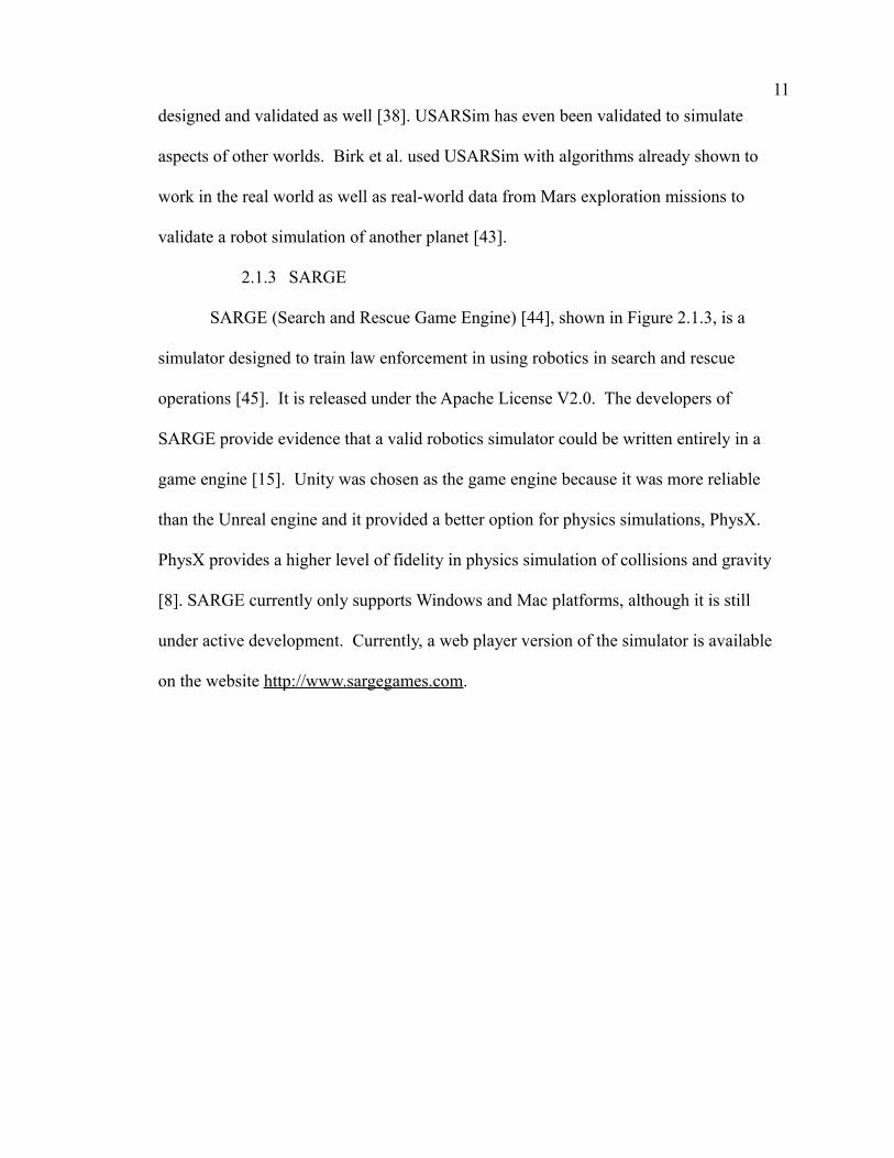
2.1.3 SARGE
SARGE (Search and Rescue Game Engine) [44], shown in Figure 2.1.3, is a
simulator designed to train law enforcement in using robotics in search and rescue
operations [45]. It is released under the Apache License V2.0. The developers of
SARGE provide evidence that a valid robotics simulator could be written entirely in a
game engine [15]. Unity was chosen as the game engine because it was more reliable
than the Unreal engine and it provided a better option for physics simulations, PhysX.
PhysX provides a higher level of fidelity in physics simulation of collisions and gravity
[8]. SARGE currently only supports Windows and Mac platforms, although it is still
under active development. Currently, a web player version of the simulator is available
on the website http://www.sargegames.com.

12
Figure 2.1.3 SARGE screenshot
It is possible for SARGE users to create their own robots and terrains with the use
of external 3D modeling software. Sensors are limited to LIDAR (Light Detection and
Ranging), 3D camera, compass, GPS, odometer, inertial measuring unit (IMU), and a
standard camera [45]. Only the GPS, LIDAR, compass and IMU are discussed in the user
manual [46]. The GPS system requires an initial offset of the simulated terrain provided
by Google Earth. The terrains can be generated independently in the Unity development
environment by manually placing 3D models of buildings and other structures on images
of real terrain from Google Earth [45]. Once a point in the virtual terrain is referenced to
a GPS coordinate from Google Earth, the GPS sensor can be used [8]. This shows that
while terrains and robots can be created in SARGE itself, external programs may be
needed to set up a full simulation.

13
2.1.4 UberSim
UberSim [47] is an open source (under GPL license) simulator based on the ODE
physics engine and uses OpenGL for screen graphics [48]. It was created in 2000 at
Carnegie Mellon University specifically with a focus on small robots in a robot soccer
simulation. The early focus of the simulator was the CMDragons RoboCup teams;
however the ultimate goal was to develop a simulator for many types and sizes of
robotics platforms [49]. Since 2007, it no longer seems to be under active development.
2.1.5 EyeSim
EyeSim began as a two-dimensional simulator for the EyeBot robotics platform in
2000 [1]. The EyeBot platform uses RoBIOS (Robot BIOS) library of functions. These
functions are simulated in the EyeSim simulator. Test environments could be created
easily by loading text files with one of two formats, either Wall format or Maze format.
Wall format simply uses four values to represent the starting and stopping point of a wall
in X,Y coordinates (i.e. x1 y1 x2 y2). Maze format is a format in which a maze is
literally drawn in a text file by using the pipe and underscore (i.e. | and _ ) as well as
other characters [50].
In 2002, the EyeSim simulator had graduated to a 3D simulator that uses OpenGL
for rendering and loads OpenInventor files for robot models. The GUI (Graphical User
Interface) was written using FLTK [2]. Test environments were still described by a set of
two dimensional points as they have no width and have equal heights [50].
Simulating the EyeBot robot is the extent of EyeSim. While different 3D models
of robots can be imported, and different drive-types (such as omni-directional wheels and
Ackermann steering) can be selected, the controller will always be based on the EyeBot

14
controller and use RoBIOS libraries [2]. This means simulated robots will always be
coded in C code. The dynamics simulation is very simple and does not use a physics
engine. Only basic rigid body calculations are used [50].
2.1.6 SubSim
SubSim [51] is a simulator for Autonomous Underwater Vehicles (AUVs)
developed using the EyeBot controller. It was developed in 2004 for the University of
Western Australia in Perth [52]. SubSim uses the Newton Dynamics physics engine as
well as Physics Abstraction Layer (PAL) to calculate the physics of being underwater
[15].
Models of different robotic vehicles are can be imported from Milkshape3D files
[52]. Programming of the robot is done by using either C or C++ for lower-level
programming, or a language plug-in. Currently the only language plug-in is the EyeBot
plug-in. More plug-ins are planned but have yet to materialize [52].
2.1.7 CoopDynSim
CoopDynSim [3] is a multi-robot simulator built on the Newton Game Dynamics
physics engine and OpenGL. It has the ability to playback simulations and even change
the rate of time for a simulation. It uses YARP middleware which uses a socket-enabled
interface. A benefit of this simulator is that each robot spawns its own thread.
CoopDynSim was designed specifically for the hardware available in the author's lab at
the Department of Industrial Electronics at the University of Minoh in Portugal.
2.1.8 OpenRAVE
OpenRAVE [53] (Open Robotics and Animation Virtual Environment) is an open
source (LGPL) software architecture developed at Carnegie Mellon University [54]. It is

15
mainly used for planning and simulations of grasping and grasper manipulations as well
as humanoid robots. It is used to provide planning and simulation capabilities to other
robotics frameworks such as Player and ROS. Support for OpenRAVE was an early
objective for the ROS team due to its planning capabilities and openness of code [55].
One advantage to using OpenRAVE is its plug-in system. Everything connects to
OpenRAVE by plug-ins, whether it is a controller, a planner, external simulation engines
and even actual robotic hardware. The plug-ins are loaded dynamically. Several
scripting languages are supported such as Python and MATLAB/Octave [53].
2.1.9 lpzrobots
lpzrobots [60] is a GPL licensed package of robotics simulation tools available for
Linux and Mac OS. The main simulator of this project that corresponds with others in
this survey is ode_robots which is a 3D simulator that used the ODE and OSG
(OpenScreenGraph) engines.
2.1.10 SimRobot
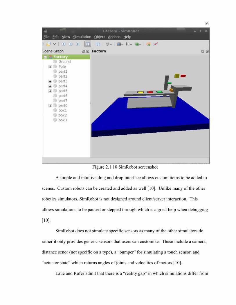
Figure 2.1.10 shows a screen shot of SimRobot [61] is a free, open source
completely cross-platform robotics simulator started in 1994. It uses the ODE for physics
simulations and OpenGL for graphics [62]. It is mainly used for RoboCup simulations,
but it is not limited to this purpose.
16
Figure 2.1.10 SimRobot screenshot
A simple and intuitive drag and drop interface allows custom items to be added to
scenes. Custom robots can be created and added as well [10]. Unlike many of the other
robotics simulators, SimRobot is not designed around client/server interaction. This
allows simulations to be paused or stepped through which is a great help when debugging
[10].
SimRobot does not simulate specific sensors as many of the other simulators do;
rather it only provides generic sensors that users can customize. These include a camera,
distance senor (not specific on a type), a “bumper” for simulating a touch sensor, and
“actuator state” which returns angles of joints and velocities of motors [10].
Laue and Rofer admit that there is a “reality gap” in which simulations differ from

17
real-world situations [62]. They note that code developed in the simulator may not
translate to real robots due to distortion and noise in the real-world sensors. They also
note, however, that code that works in the real world may completely fail when entered
into the simulation because it may rely on that distortion and noise. This was specifically
noted with the camera sensor and they suggested several methods to compensate for this
difference [62].
2.1.11 Moby
Moby [63] is an open source (GPL 2.0 license) rigid body simulation library written in
C++. It supports Linux and Mac OS X only. There is little documentation for this
simulation library.
2.1.12 Comparison of Open Source Simulation Tools
Table 2.1.13 shows the relative advantages and disadvantages of the simulators
covered in this section [64].
Table 2.1.13. Comparison of open source simulatorsSimulator Advantages Disadvantages
Stage/Gazebo
• Open Source (GPL)• Cross Platform• Active Community of Users
and Developers• Uses ODE Physics Engine for
High Fidelity Simulations• Uses TCP Sockets• Can be Programmed in Many
Different Language
USARSim
• Open Source (GPL)• Supports both Windows and
Linux• Users Have Ability to Make
Custom Robots and Terrain with Moderate Ease
• Uses TCP Sockets• Can be Programmed in Many
Different Language
• Hard to Install• Must have Unreal
Engine to use (Costs about $40)
• Uses Karma Physics Engine

18
Table 2.1.13 ContinuedSimulator Advantages Disadvantages
SARGE
• Open Source (Apache License V2.0 )
• Uses PhysX Physics Engine forHigh Fidelity Simulations
• Supports both Windows and Mac
• Users Have Ability to Make Custom Robots and Terrain with Moderate Ease
• Uses TCP Sockets• Can be Programmed in Many
Different Languages
• Designed for Training, not Full Robot Simulations
UberSim• Open Source (GPL)• Uses ODE Physics Engine for
High Fidelity Simulations
• No Longer Developed
EyeSim • Can Import Different Vehicles• Only Supports
EyeBot Controller
SubSim
• Can Import Different Vehicles• Can be programmed in C or
C++ as well as using plug-ins for other languages
CoopDynSim • Multi-Robot system• Multithreaded• Uses YARP to interface via
TCP socketsOpenRAVE • Open Source (Lesser GPL)
• Everything Connects using plug-Ins
• Can be used with Other Systems (like ROS and Player)
• Can be Programmed in SeveralScripting Languages
lpzrobots • Open Source (GPL)• Uses ODE Physics Engine for
High Fidelity Simulations
• Linux and Mac only
SimRobot • Open Source• Users Have Ability to Make
Custom Robots and Terrain Moby
• Open Source (GPL 32.0)• Written in C++
• Supports Linux and Mac only
• Very little documentation
19
2.2 Commercial Simulators
There are many commercial robotics simulators available. The commercial
simulators described and compared in this paper will be focused on research and
education.
As with any commercial application, one downfall of all of these applications is
that they typically are not open source. Commercial programs that do not release source
code can tie the hands of the researcher, forcing them in some cases to choose the less
than optimal answer to various research questions. When problems occur with
proprietary software, there is no way for the researcher to fix it. This problem alone was
actually the impetus for the Player Project [65].
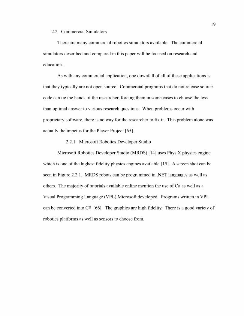
2.2.1 Microsoft Robotics Developer Studio
Microsoft Robotics Developer Studio (MRDS) [14] uses Phys X physics engine
which is one of the highest fidelity physics engines available [15]. A screen shot can be
seen in Figure 2.2.1. MRDS robots can be programmed in .NET languages as well as
others. The majority of tutorials available online mention the use of C# as well as a
Visual Programming Language (VPL) Microsoft developed. Programs written in VPL
can be converted into C# [66]. The graphics are high fidelity. There is a good variety of
robotics platforms as well as sensors to choose from.

20
Figure 2.2.1 Microsoft Robotics Developer Studio screenshot
Only computers running Windows 7 are supported in the latest release of MRDS,
however, it can be used to program robotic platforms which may run other operating
systems by the use of serial or wireless communication (Bluetooth, WiFi, or RF Modem)
with the robot [67].
2.2.2 Marilou
Figure 2.2.2 shows a screen shot of Marilou by anyKode [68]. Marilou is a full
robotics simulation suite. It includes a built in modeler program so users can build their
own robots using basic shapes. The modeler has an intuitive CAD-like interface. The
physics engine simulates rigid bodies, joints, and terrains. It includes several types of
available geometries [69]. Sensors used on robots are customizable, allowing for specific

21
aspects of a particular physical sensor to be modeled and simulated. Devices can be
modified using a simple wizard interface.
Figure 2.2.2 anykode Marilou screenshot
Robots can be programmed in many languages from Windows and Linux
machines, but the editor and simulator are Windows only. Marilou offers programming
wizards that help set up projects settings and source code for based on which language
and compiler is selected by the user [70].
Marilou is not open source or free. While there is a free home version, it is meant
for hobbyists with no intention of commercialization. The results and other associated
information are not compatible with the professional or educational versions. Prices for
these versions range from $360 to $2,663 [71].
22
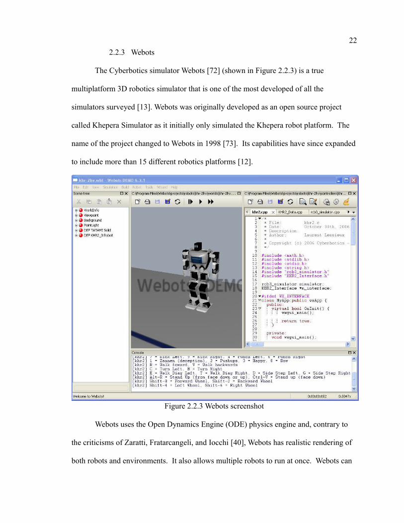
2.2.3 Webots
The Cyberbotics simulator Webots [72] (shown in Figure 2.2.3) is a true
multiplatform 3D robotics simulator that is one of the most developed of all the
simulators surveyed [13]. Webots was originally developed as an open source project
called Khepera Simulator as it initially only simulated the Khepera robot platform. The
name of the project changed to Webots in 1998 [73]. Its capabilities have since expanded
to include more than 15 different robotics platforms [12].
Figure 2.2.3 Webots screenshot
Webots uses the Open Dynamics Engine (ODE) physics engine and, contrary to
the criticisms of Zaratti, Fratarcangeli, and Iocchi [40], Webots has realistic rendering of
both robots and environments. It also allows multiple robots to run at once. Webots can

23
execute controls written in C/C++, Java, URBI, Python, ROS, and MATLAB languages
[74]. This simulator also allows the creation of custom robotics platforms; allowing the
user to completely design a new vehicle, choose sensors, place sensors where they wish,
and simulate code on the vehicle.
Webots has a demonstration example showing many of the different robotics
systems it can simulate, including an amphibious multi-jointed robot, the Mars Sojourner
rover, robotic soccer teams, humanoids, multiple robotic arms on an assembly line, a
robotic blimp, and several others. The physics and graphics are very impressive and the
software is easy to use.
Webots has a free demonstration version available (with the ability to save world
files crippled) for all platforms, and even has a free 30 day trial of the professional
version. The price for a full version ranges from $320 to $4312 [75].
2.2.4 robotSim Pro/robotBuilder
robotBuilder [72] is a software package from Cogmation Robotics that allows
users to configure robots models and sensors. Users import the models of the robots,
import and position available sensors onto the robots, and link these sensors to the robot's
controller. Users can create and build new robot models piece by piece or robotBuilder
can import robot models created in other 3D CAD (Computer-Aided Design) programs
such as the free version of Google Sketchup. The process involves exporting the
Sketchup file as a COLLADA or 3DS file, then importing this into robotBuilder [73].

24
Figure 2.2.4 robotSim Pro screenshot
robotSim Pro (seen in Figure 2.2.4) is an advanced 3D robotics simulator that uses
a physics engine to simulate forces and collisions [76]. Since this software is commercial
and closed source, the actual physics engine used could not be determined. robotSim
allows multiple robots to simulate at one time. Of all of the simulators in this survey,
robotSim has some of the most realistic graphics. The physics of all objects within a
simulation environment can be modified to make them simulate more realistically [76].
Test environments can be easily created in robotSim by simply choosing objects to be
placed in the simulation world, and manipulating their positions with the computer
mouse. Robot models created in the robotBuilder program can be loaded into the test
environments. Virtual robots can be controlled by one of three methods; the Cogmation

25
C++ API, LabVIEW, or any socket-enabled programming language [77].
robotSim is available for $499 or as a bundle with robotBuilder for $750.
Cogmation offers a 90-day free trial as well as a discounted academic license.
2.2.5 Comparison of Commercial Simulators
Table 2.2.5 is a comparison of the relative advantages and disadvantages of the
specific commercial simulators mentioned in this survey.
Table 2.2.5. Comparison of commercial robotics simulatorsSimulator Advantages Disadvantages
Microsoft Robotics Developer Studio
• Visual Programming Language• Uses PhysX Physics Engine for
High Fidelity Simulations• Free
• Installs on Windows Machines only
• Not Open SourceMarilou • Users Have Ability to Make
Custom Robots and Terrain Using Built-in Modeler
• Provides Programming Wizards
• Robots Can be Programmed in Windows or Linux
• Free Home Version Available
• Installs on Windows Machines only
• Not Open Source• License Costs
Range between $260 and $2663
Webots • Uses ODE Physics Engine for High Fidelity Simulations
• Can be Programmed in Many Different Languages
• Free Demonstration Version Available
• Not Open Source• License Costs
Between $320 and$4312
robotSim /robotBuilder • Users Have Ability to Make Custom Robots and Terrain Using Built-in Modeler
• Uses TCP Sockets• Can be Programmed in Many
Different Languages• 90-day Free Trial and
Discounted Academic License Available
• Not Open Source• License Costs
Between $499 and$750
2.3 Middleware
Middleware is software that sits between the user-written control code and the
target hardware such as a robot (whether it be simulated or real hardware). The reason

26
middleware exists is to allow for highly abstracted interactions between multiple types of
hardware and software. For instance, in many cases the user doesn't have to change their
code if they move from a simulator to a real robot, or even between different types of
robotic vehicles. Middleware also allows for access to third-party software libraries for
advanced features such as path planning, localization, mapping, computer vision, etc. It
can act as a kind of “switch-board” to direct messages to and from different libraries and
hardware. Several types of middleware were considered during this survey.
2.3.1 Player Project Middleware
Player is a TCP socket enabled middleware that is installed on the robotic
platform [20]. This middleware creates an abstraction layer on top of the hardware of the
platform, allowing portability of code [65]. Being socketed allows the use of many
programming languages [27]. While this may ease programming portability between
platforms it adds several layers of complexity to any robot hardware design.
To support the socketed protocol, drivers and interfaces must be written to interact
with each piece of hardware or algorithm. Each type of sensor has a specific protocol
called an interface which defines how it must communicate to the driver [78]. A driver
must be written for Player to be able to connect to the sensor using file abstraction
methods similar to POSIX systems. The robotic platform itself must be capable of
running a small POSIX operating system to support the hardware server application [25].
This is overkill for many introductory robotics projects, and its focus is more on higher
level aspects of robotic control and users with a larger budgets. The creators of Player
admit that it is not fitting for all robot designs [27].
Player currently supports more than 10 robots as well as 25 different hardware

27
sensors. Custom drivers and interfaces can be developed for new sensors and hardware.
The current array of robots and sensor hardware available for Player can be seen on the
Player project’ s supported hardware web page [24].
2.3.2 ROS (Robot Operating System)
ROS [79] is currently one of the most popular robotics middleware systems. Only
UNIX-based platforms are officially supported (including Mac OS X) but the company
Robotics Equipment Corporation has ported it to Windows [80]. ROS is fully open source
and uses the BSD license [11]. This allows users to take part in the development of the
system, which is why it has gained wide use. In its meteoric rise in popularity, over the
last three years it has added over 1643 packages and 52 code repositories since it was
released [81].
One of the strengths of ROS is that it interfaces with other robotics simulators and
middleware. It has been successfully used with Player, YARP, Orcos, URBI,
OpenRAVE, and IPC [82]. Another strength of ROS is that it can incorporate many
commonly used libraries for specific tasks instead of having to have its own custom
libraries [11]. For instance, the ability to easily incorporate OpenCV has helped make
ROS a better option than some other tools. Many libraries from the Player project are
also being used in certain aspects of ROS [65]. An additional example of ROS working
well with other frameworks is the use of the Gazebo simulator.
ROS is designed to be a partially real-time system. This is due to the fact that the
robotics platforms it is designed to be used, like the PR2, will be in situations involving
more human-computer interaction in real time than many current commercial research
robotics platforms. One of the main platforms used for the development of ROS is the

28
PR2 robot from Willow Garage. The aim of using ROS’s real-time framework with this
robot is to help guide safe Human-Robot Interaction (HRI). Previous frameworks such as
Player were rarely designed with this aspect in mind.
ROS is made up of many separate parts, namely the ROScore and ROSnodes. The
ROScore is like a switchboard. It routes messages between other ROSnodes. “ROSnode”
is a term used to describe other applications that either send or receive ROS messages.
Figure 2.3.2 shows an example ROS project.
Figure 2.3.2 Simplified ROS application
In the example shown in Figure 2.3.2, all of the bubbles attached to the ROScore
directly are ROSnodes. The code that the user writes must implement a ROSnode to be
able to send messages to the ROScore. The Roomba and arduino nodes can be thought of
as device drivers and have two interfaces. One side interfaces with ROScore and sends
and receives ROS-standard message types. The other side connects via serial ports to
either physical hardware, or a simulator depending on how the user has configured the
project. The Roomba node converts ROS-standard “drive” message-types (a “twist”

29
message) into Roomba protocol commands and sends them to a physical Roomba robot.
The arduino node converts ultrasonic sensor values into the ROS-standard “range”
message-type when gets forwarded to the user's code. The user's code can be written in
one of several different ROS-supported languages. It receives sensor information from
the Roomba and arduino nodes via the ROScore (shown in Figure 2.3.2 by the red and
blue arrows). The code then processes the sensor data to derive an appropriate drive
command. This drive command is a standard ROS message-type called a “twist” (the
black arrow in Figure 2.3.2). It is then sent to the ROScore and routed to the
RoombaNode. The Roomba node converts the twist message into the standard Roomba
protocol command and sends it to the actual Roomba hardware via serial connection. The
hardware abstraction layer in Figure 2.3.2 can be replaced by a simulator, and the rest of
the software would not “know” the difference.
2.3.3 MRL (MyRobotLab)
MRL (seen in Figure 2.3.3.1) is a Java middleware that includes many third-party
libraries and hardware interfaces [83]. It is written as a service-based architecture that
includes both graphical and textual control of the services and their interconnections. A
python interpreter gives the user complete access to all public classes in all the services
of MRL. This allows for users to design complex systems in a single python script file.
Recently, a Java service has been implemented in MRL which will also become useful for
users once it is more mature. MRL is actively developed, and the developer is generally
available for consultation through the MRL website.

30
Figure 2.3.3.1 A screenshot of the main MRL window displaying several importantservices that are available to the user.
Figure 2.3.3.2 shows a typical project in MRL using an actual Roomba vehicle.
The user's code is written in MRL's python interpreter. MRL uses the open source
RoombaComm Java library to communicate to Roomba hardware. The user can initiate a
RoombaComm service either manually using the MRL GUI or in the python interpreting
service. This service then connects to an actual Roomba using a serial port. Sensor and
drive messages are defined in the Roomba's native protocol (as defined in [84]).

31
Figure 2.3.3.2 A typical project in MRL using an actual Roomba vehicle.
2.3.4 RT Middleware
RT Middleware [85] is set of standards used to describe a robotics framework.
The implementation of these standards is OpenRTM-aist, which is similar to ROS. This
is released under the Eclipse Public License (EPL) [86]. Currently it is available for
Linux and Windows machines and can be programmed using C++, Python and Java [85].
The first version of OpenRTM-aist (version 0.2) was released in 2005 and since then its
popularity has grown. Version 1.0 of the framework was released in 2010.
OpenRTM-aist is popular in Japan, where a lot of research related to robotics
takes place. While it does not provide a simulator of its own, work has been done to
allow compatibility with parts of the Player project [87].
2.3.5 Comparison of Middleware
Table 2.3.5 compares the relative advantages and disadvantages of the open
source middleware discussed in this survey.

32
Table 2.3.5. Comparison of open source middlewareSimulator Advantages Disadvantages
Player
• Open Source (GPL)• Cross Platform• Active Community of Users
and Developers• Uses TCP Sockets• Can be Programmed in Many
Different Language
• Every physical hardware device must use TCP protocol
ROS
• Open Source (BSD License) • Supports Linux, Mac, and
Windows*• Very Active Community of
Users and Developers • Works with Other Simulators
and Middleware
• Very complicated to learn and to use
MRL (MyRobotLab)
• Open source• Completely Java based,
making it able to run on Linux,Windows, Mac, Android and even in web browsers
• Very easy to learn and use• Active community of
developers• Interfaces with a multitude of
common third-party libraries, software, and hardware
• Very easy to customizeRT-Middlware • Open Source (EPL)
• Based on a Set of Standards that are Unlikely to Change Dramatically
• Works with Player Project• Can be Programmed in Several
Different Languages
2.4 Conclusion
While this is certainly not an exhaustive list of robotics simulators and tools, this
is a simple comparison of several of the leading simulator packages available today.
Most of the simulators in this survey are designed for specific robotics platforms
and sensors which are quite expensive and not very useful for simpler, cheaper systems.
The costs and complexities of these systems often prevent them from being an option for

33
projects with smaller budgets. The code developed in many of these simulators requires
expensive hardware when porting to real robotics systems. The middleware that is
required to run on actual hardware is often too taxing for smaller, cheaper systems. There
simply isn't a very good 3D robotics simulator for custom robotic systems designed on a
tight budget. Many times a user only needs to simulate simple sensor interactions, such
as simple analog sensors, with high fidelity. In these cases, there is no need for such
processor intensive, high abstraction simulators.

CHAPTER 3: HISTORY OF SEAR
3.1 Overview of SEAR Concept
The concept of SEAR was conceived as a free (completely open source), cross
platform, and 3D graphically and physically accurate robotics simulator. The proposed
simulator is able to import 3D, user-created vehicle models and real-world terrain data.
The SEAR simulator is easy to setup and use on any system. The source code is freely
available which entices collaboration from the open source community. The simulator is
flexible for the user and is intuitive to use for both the novice and the expert.
SEAR began as a thesis project which laid the groundwork for a tool that matched
the concept requirements [64]. Since its inception, SEAR has gone through multiple
iterations as features were either added or removed and as sensors were validated.
3.2 Initial Design
In the initial design of SEAR, the models of robotic vehicles were imported into
the simulator in Ogre mesh format. These models were created using one of the many 3D
modeling CAD software programs. Terrain models could be created either externally in
CAD and imported into the simulator, or coded directly in jME. One method for creating
real-world terrains is by importing from Google Earth. This model can then be used as
the basis for a fully simulated terrain as can be seen in Figure 3.2.
35
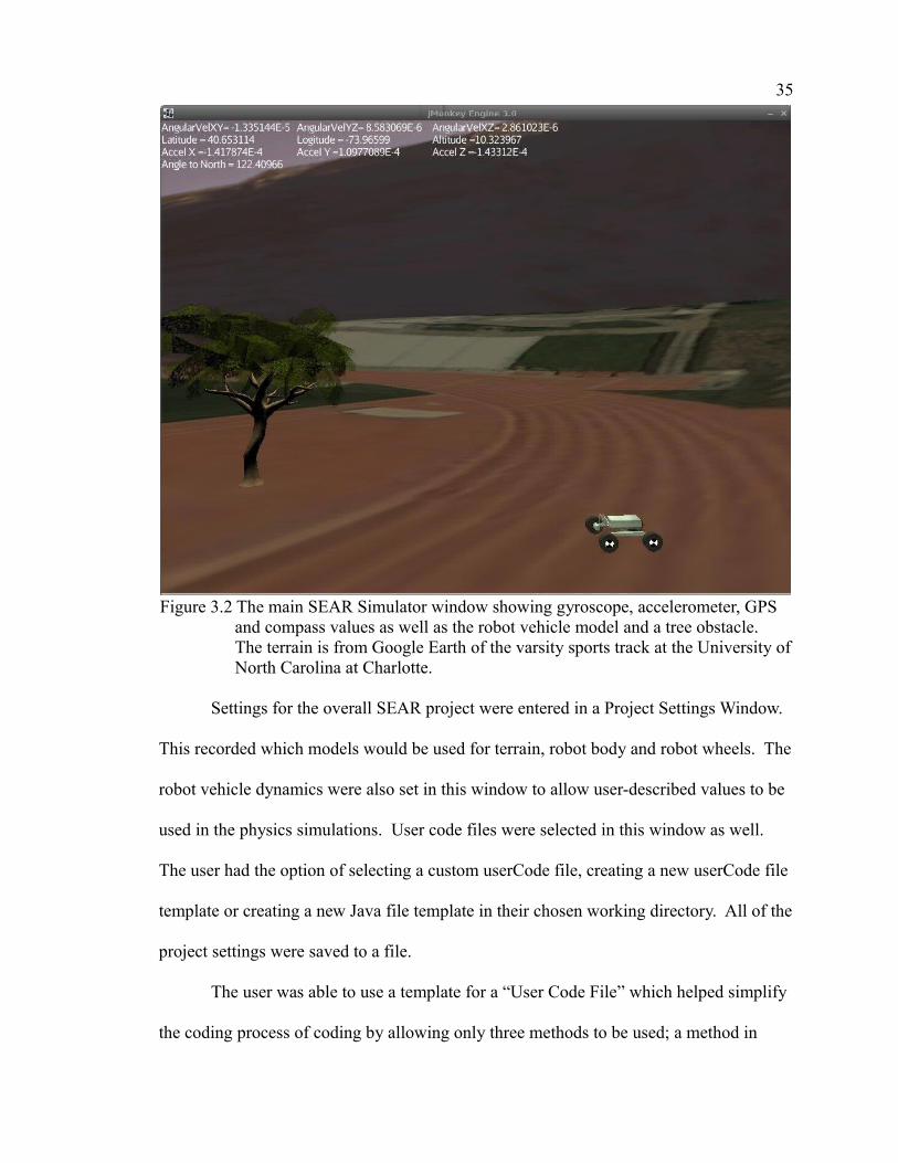
Figure 3.2 The main SEAR Simulator window showing gyroscope, accelerometer, GPS and compass values as well as the robot vehicle model and a tree obstacle. The terrain is from Google Earth of the varsity sports track at the University ofNorth Carolina at Charlotte.
Settings for the overall SEAR project were entered in a Project Settings Window.
This recorded which models would be used for terrain, robot body and robot wheels. The
robot vehicle dynamics were also set in this window to allow user-described values to be
used in the physics simulations. User code files were selected in this window as well.
The user had the option of selecting a custom userCode file, creating a new userCode file
template or creating a new Java file template in their chosen working directory. All of the
project settings were saved to a file.
The user was able to use a template for a “User Code File” which helped simplify
the coding process of coding by allowing only three methods to be used; a method in

36
which users can declare variables, an initialization method and a main loop method. This
was designed to reduce confusion for novice users and makes prototyping a quick and
easy process. Additionally, the user could choose to code from a direct Java template of
the simulator itself. This would be a preferred method for more advanced simulations.
Upon starting a simulation, the values recoded in the project settings file (.prj)
created in the Project Settings Window and the userCode file (.ucf) were used to create
the simulator Java file by copying and pasting the user code to the appropriate sections of
the simulator Java template. This file was then compiled and the resulting application was
run to perform the simulation. Every time the simulator ran, it had to be completely
recompiled. Though this was hidden from the user, it proved to be a complicated and
messy implementation. There was no error console, so if the user code caused an error,
there was no feedback from the compiler to explain why the compilation failed.
3.3 Intermediate Designs (Graduate Work)
SEAR has gone through many intermediate designs, including interfacing with
multiple middleware suites as well as testing multiple communication protocols to
validate which would be best to utilize. Concurrently, previously created sensors were
improved, new classes of sensors were added and validated against actual hardware.
3.3.1 Early ROS Middleware Integration
A new class of sensors, “visual sensors,” was added which included ultrasonic
sensors. The creation and validation of the technique used for simulating this new class
of sensors meant that SEAR would have to change drastically. The new sensors were
validated (proven to act similarly to physical sensors in a similar physical environment)
against both real world sensors and another simulator (Stage). In order to keep as many

37
variables in the testing of the SEAR sensor as consistent as possible with the physical
experiment as well as in the Stage simulation experiment a middleware, ROS, was
selected to interface with each system. This allowed the same robot control code to be
used on all three platforms: SEAR, real-world hardware, and Stage. Additionally, the
Roomba robot was chosen as the vehicle because the iRobot Roomba is nearly
universally supported by many robotics simulators and middleware. Only indoor
environments were used for testing to reduce the number of variables introduced. The
odometer sensor was created to allow for a second measure in the validation of the visual
sensor class.
Since the focus of SEAR changed to the validation of sensors, many of the
previous features had to be removed. The model-loading for terrain was no longer
needed as it was simpler to build the environments within jME3 by hand. Similarly, the
ability to load custom robotic vehicles was removed. Hard-coded environments and
vehicles reduced the time between simulations and reduced the number of files associated
with a given project. The removed features were later added back into SEAR.
User-code integration was completely removed and in its place, a separate ROS
communications thread was used. This allowed SEAR to send and receive standard ROS
message-types. Because of this simplification, there was no need to dynamically create
and compile the SEAR simulation each time it ran.
Simulation no longer required the project settings GUI since all the settings were
hard-coded. The sensor wizard XML files were also no longer required. The distance
sensor class was validated in SEAR utilizing only the main simulation class, the sensor
simulator classes, and the ROS communications thread.

38
3.3.2 Early MRL Integration
After the sensors were validated, the focus was moved toward integration with a
simpler middleware called MyRobotLab (MRL). The main reason for this change is the
immaturity of the Java-based implementation of ROS. ROSJava, as it was called,
changed so rapidly that the code used in the validation was completely deprecated by the
time the validation was finished. Instead of starting from scratch on ROS integration, the
change to MRL allowed for a more stable development platform over time.
The first integration with MRL used a client library called the MRLClient. It
began as a UDP messaging service that communicated with a running instance of MRL.
Shortly after implementation, the protocol was changed to TCP to reduce the amount of
packet loss between the two programs. This was still not an ideal solution as it was slow
and often times had errors. Eventually, SEAR was incorporated directly with MRL with
the creation of a SEAR service inside MRL. This allowed for communication between
MRL services to be very easy.
During the same time as the MRL integration, the LIDAR simulator was
implemented and then verified against actual hardware. Once all of the sensors were
finished, they were combined into a single Java package that could interact together in
the same simulation. The simulators were moved to execute in the physics thread of jME
rather than the simpleUpdate() method. This increased the speed of simulations.
The creation of environments (models of terrain and obstacles) inside SEAR was
added to the MRL SEAR service. This involved the creation of many new classes of
environment object-types such as Box, Cylinder and Cone objects. These objects can be
created in python code inside MRL and are stored in the main SEAR project folder as

39
XML files. This development meant that environments were no longer hard-coded into
SEAR; they could be changed easily.
SEAR currently supports “robot objects” which communicate using the iRobot
Roomba Create Open protocol [84]. This protocol was chosen because the Roomba
protocol is widely used and very simple to implement on practically any hardware. In
fact, the drive commands from the iRobot protocol use a common interface that Eyesim
authors refer to as “omega-v” which specifies both the linear and angular velocity the
robot should obtain [1], [2]. Custom protocols could also be used with SEAR, however
the user would have to write a “customController” SEAR object script to handle
communications and drive the virtual robot.
3.4 Conclusion
As shown in this section, the growth of SEAR allowed for experimentation of
each important aspect previously defined for a good modern simulator. Middleware
integration was explored by interfacing with ROS and later with MRL. Different
methods of communication were explored as well. Simulations of sensors were
improved and validated against physical hardware to prove the simulated outputs closely
matched the results of the actual sensors they were modeled on. The final iteration of
SEAR is described in detail in the following chapters.

CHAPTER 4: SUPPORTING DESIGN TOOLS
This research relied on several software tools for development. The required
software ranged from integrated development environments (IDEs) to 3D modeling CAD
software. Netbeans 6.9 was used for coding Java for the project. The game engine used
was jMonkeyEngine3 (jME3). A survey of different modeling software was performed to
show the variety available to the user [64].
4.1 Language Selection
Using previous surveys of current robotics simulators [15], [21], [23] it was
shown that several of the current systems claim to be cross platform. While this may
technically be true, it is often so complicated to implement these systems on different
platforms that most people would rather switch platforms than spend the time and effort
trying to setup the simulators on their native systems. Most of the currently available
open source simulator projects are based on C and C++. While many of these are
considered also cross-platform, getting them running correctly requires so many work-
arounds and special configurations that it is often more efficient to change the
development hardware to match the recommended hardware of the simulators.
To make a simulator easy to use as well as to simplify further development, Java
was selected as the language to code the simulator. Java runs in a virtual machine on a
computer. This abstraction prevents the Java code from having to directly interface with
any hardware, allowing the Java code to be unchanged regardless of what hardware it is

41
run on. The development platform used was NetBeans 6.9.
4.2 Game Engine Concepts
The jME3 game engine consists of two major parts, each with their own “spaces”
that must be considered for any simulation. The first is a “graphics world space” (called
the “scene graph”) which is controlled by the rendering engine and displays all of the
screen graphics. The scene graph is created by jMonkeyEngine in this project.
The second space, the “physics world space,” is controlled by the physics engine
which can simulate rigid body dynamics, fluid dynamics, or other dynamic systems.
Currently in SEAR, only rigid body dynamics are being used. The physics engine
calculates interactions between objects in the “physics space” such as collisions, as well
as variations in mass and gravity.
A developer must think about both the graphics and physics spaces concurrently
as each runs in its own thread. It is possible for objects to exist in only one of these
spaces which can lead to simulation errors. Once an object is made in the graphics space,
it must be attached to a model in the physics space in order to react with the other objects
in the physics space. For instance, an obstacle created in only the graphics space will
show up on the screen during a simulation, however, the robot can drive directly through
the obstacle without being affected by it. Conversely, the obstacle can exist only in the
physics space. A robot in this instance would bounce off of an invisible object in a
simulation. Another issue would be to have an obstacle created in both spaces, but not in
the same place. This would lead to problems such as the robot driving though the visible
obstacle, and running into its invisible physics model a few meters behind the obstacle.
Attention must be paid to attach both the graphics objects and physics objects correctly.
42
The game engine creates a 3D space or “world.” In each direction (X, Y and Z)
the units are marked as “world units.” The Bullet physics engine (the one implemented
in jME3) treats one world unit as one meter [88]. Certain model exporters will have a
scale factor; however that can be used to change the units of the model upon export.
Additionally, any object can also be scaled inside the game engine.
4.3 JmonkeyEngine Game Engine
The game engine selected for this project was jMonkeyEngine3 (jME3) since it is
a high performance, truly cross platform Java game engine. The basic template for a
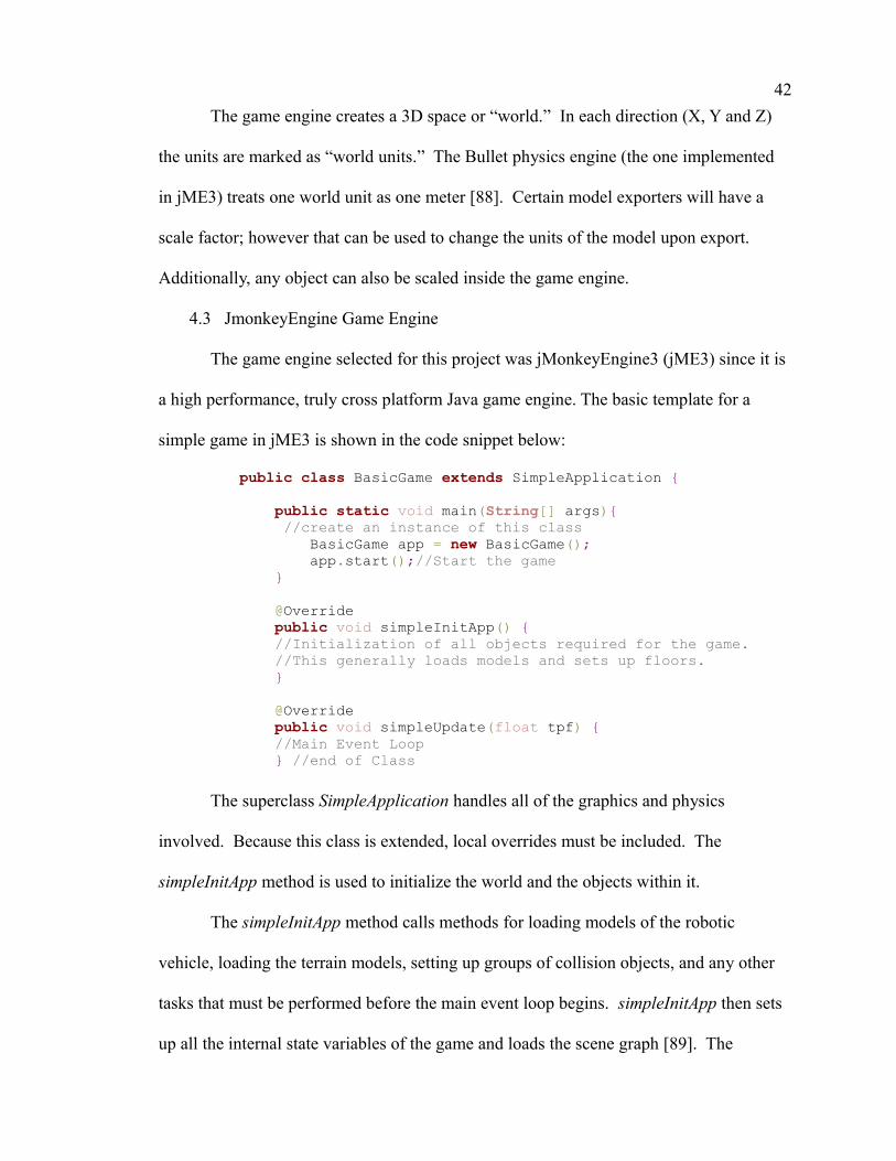
simple game in jME3 is shown in the code snippet below:
public class BasicGame extends SimpleApplication { public static void main(String[] args){ //create an instance of this class BasicGame app = new BasicGame(); app.start();//Start the game }
@Override public void simpleInitApp() { //Initialization of all objects required for the game. //This generally loads models and sets up floors. }
@Override public void simpleUpdate(float tpf) { //Main Event Loop } //end of Class
The superclass SimpleApplication handles all of the graphics and physics
involved. Because this class is extended, local overrides must be included. The
simpleInitApp method is used to initialize the world and the objects within it.
The simpleInitApp method calls methods for loading models of the robotic
vehicle, loading the terrain models, setting up groups of collision objects, and any other
tasks that must be performed before the main event loop begins. simpleInitApp then sets
up all the internal state variables of the game and loads the scene graph [89]. The

43
simpleUpdate method is the main event loop. This method is an infinite loop and is
executed as quickly as possible. This is where important functions of the simulator
reside. Additionally, other methods from the simpleBulletApplication may be overridden
such as onPreUpdate and onPostUpdate, though these were not used specifically in this
project.
jME3 uses the JBullet physics engine for physics calculations. JBullet is a one-
hundred percent Java port of the Bullet Physics Library which was originally written in
C++. There is a method in SimpleApplication specifically for handling the physics called
“physicsTick()”. This is the method in which the sensors of SEAR are simulated. jME3
allows the physics to be handled in a separate thread from the graphics.
Objects in jME3 must be represented both graphically as well as physically to
work in a simulation. Simulating sensors in SEAR also requires utilizing both the
graphics and physics threads almost simultaneously. Data must be passed between the
threads to calculate graphical representations of sensor components as well as the virtual
robot's position within the virtual environment. This is similar to the CoopDynSim
simulator [3]. Figure 4.3 is a representation of roughly how the threads communicate.
Figure 4.3 Data for each sensor simulator is shared between graphics and physics threads in SEAR

CHAPTER 5: ARCHITECTURE AND METHODS OF IMPLEMENTATIONUTILIZED TO CREATE SEAR
This section describes the implementation of the virtual sensors within SEAR, the
architecture of SEAR, communication between SEAR and middleware (MRL), and the
organization of a end-user's files related to a single simulation project from the
perspective of a developer of SEAR. Typical end-user interactions can be found in
Appendix A which has example code listings for how to create and use every
environment object (terrain and obstacles) as well as robot components (boxes, cylinders,
wheels, robot dynamics settings, and sensors).
For perspective, it is useful to understand where each of the components of SEAR
fit in an example of a typical user project. In this example, the user will utilize MRL's
python service to control a virtual robot and communicate with sensors. One of each
sensor will be used. As a comparison the same project is shown twice; one implemented
with physical hardware (shown in Figure 5a), and then again using the SEAR simulator
(shown in Figure 5b). The portions that were created by the author of this dissertation for
the SEAR simulator are shown by the text being preceded by an asterisk (*).

45
Figure 5.0 (a) A typical project using MRL to control a physical robot. (b) The same project interfacing instead with SEAR. The blue arrows are MRL system messages, the Red arrows are serial or virtual serial ports and the orange arrow is a direct JAVA method call from MRL to SEAR. The items with an asterisk (*) denote modules written by the author of this dissertation.
5.1 The SEARproject
The concept of a “SEARproject” was devised to allow users to contain all the files
of a single project together. It is similar in structure to how word processor documents
save text, formatting and associated files to a computer hard drive. This structure will
allow users to share aspects of their projects, be it code, entire environments, or entire
robot models (complete with sensor specifics).
The SEARproject is created when the user creates objects using a custom library.
This creates a folder within MRL’’s operating environment called “SEARproject.”

46
Environment objects are stored in a subfolder named “environment,” robot components
are stored in a subfolder named “robot,” and all the files associated with user-created
CAD files of objects or any images the user selects to wrap around SEAR-native objects
are located in a folder named “assets.” Users' Python or Java code can be stored in the
SEARproject folder.
When the user is ready to save the SEARproject, this folder is compressed in ZIP
format, and renamed with the file extension “.sear” to designate it as a sear project. This
can then be opened at a later time from the MRL SEAR service GUI window, or shared
with other users. Figure 5.1 illustrates the file structure inside a .sear file.
Figure 5.1 Folder tree showing the layout of a SEARproject
MRL's SEAR service has options to save and open .sear files. Projects are stored
in MRL's working directory in a folder named “SEARproject” until they are saved.
When the user saves a file, the SEAR service zips SEARproject folder and saves it as a
.sear file at the given path and file name the user enters.
5.2 Custom MRL Services
Several MRL services were created to allow SEAR and its virtual robots and
sensor objects to communicate with MRL. Additionally, MRL did not support several
standard sensor types for physical sensors. Custom services were written to add LIDAR
and GPS sensors to MRL, as well as a service used to interface MRL with the SEAR
simulator. These services can interface with actual hardware or simulated hardware [90].

47
5.2.1 MRL'S LIDAR Service
Figure 5.2.1 The LIDAR service GUI panel showing the output of
an actual SICK LMS-200 scan
MRL did not have a service for interfacing with LIDAR devices at the time of this
research, so one was created. The service currently handles SICK LMS-200 devices and
can be used to set up and receive scan data [91]. Once a scan is performed, the resulting
values are parsed and displayed on the LIDAR service GUI panel in MRL in polar form
(with the senor location being at the center of the bottom of the display). Figure 5.2.1
shows a resulting LIDAR scan. This service was first tested with an actual SICK LMS-
200 LIDAR unit to verify functionality. LIDAR messages are called “telegrams” in the
SICK documentation [91]. Many telegrams are currently supported with the exception of
the “streaming” scan mode. Users can get similar functionality by putting the single scan
function call within a loop to perform multiple scans. The user has the ability to change
the resolution of the scans and the speed of the serial communications using standard

48
LMS-200 telegrams [92]. All functions are currently only available to the user if they use
the Python or Java MRL services.
5.2.2 MRL's GPS Service
MRL did not have a GPS service at the time of this research, so one was created.
The service utilized other portions of MRL’s serial service to parse values from a GPS
NMEA string. Currently, only GPGGA strings in the format used by the San Jose FV-M8
are supported as they are the most useful for the SEAR simulator at this time and the only
physical hardware available to test [93]. The MRL GPS service parses the GPGGA string
and displays the values in the GPS service GUI panel, and allows the user to access this
data directly from the GPS service via Python or Java code. Figure 5.2.2 shows the GPS
GUI.
Figure 5.2.2 The GPS panel of MRL’s GPS service GUI showing values from a simulated GPS device
5.3 MRL'S SEAR Service
The SEAR service has a GUI portion that allows users to open or save SEAR
project files, and start a SEAR simulation. Most of its functionality is not available on
the GUI window. The SEAR service orchestrates all the serial communications between
the software serial ports (virtualSerialPort services within MRL).
5.4 SEAR's Object Grammar
A custom grammar was created to allow users to design environments, obstacles
and robot components using SEAR-native objects. This is accomplished by the

49
SEAR.POJO library that was added to MRL. The user must import the “SEAR.POJOs”
library within MRL's Python or Java service in order to create these objects. A POJO is a
“Plain Old Java Object” which is a Java object that is devoid of methods and simply
holds information. It can be thought of as similar to a “structure” in C language. By
default, when the user creates these POJO objects, they are immediately serialized as
XML files.
SEAR objects include graphical and physical representations of boxes, cylinders,
and cones as well as components specific to a robot such as dynamics, sensors and
wheels. Sensor objects are used to set up the specific settings of a particular sensor type
such as communication settings, resolution, and type. Tables 5.4.1 and 5.4.2 list the
different types of objects supported by the POJO library.
Table 5.4.1. Physical objects in the SEAR POJOs libraryObjects Description
Box Cone A cone shape with a default image of a traffic cone
Floor
Cylinder A cylinder with a default image of a recycling bin
Model
Wheel
A rectangular prism with a default image of a cardboard box
A rectangular prism that can be ignored by distance and LIDAR sensors
A 3d model the user created outside of MRL and SEAR usually in OGRE mesh format. This can include custom images and textures. Additionally, Blender .blend files can be used.A special cylinder object that is specifically used as a robot component. The user can select whether this wheel is connected to the motor or if it is an idler.

50
Table 5.4.2. Sensor objects in the SEAR simulator POJOs libraryObjects Description
SEARrobot
3-axis Accelerometer
Compass Sensor
Distance
Robot Dynamics
GPS
3-axis GyroscopeLIDAR Simulates Laser ranging devices, named the SICK LMS200
Odometer
This is an object that represents a “robot” entity. Other physical and sensor objects are added to this entity to create the physical representation as well as the sensor payload of the robot.Measures acceleration in 3 dimensions relative to the robot's bodyMeasures angle to “north” which defaults to 1000km in the X axis unless magnetic declination is selected (automatically calculated based on the robot's GPS coordinates)This sensor is highly configurable and can simulate SONAR, RADAR, Infrared, simple laser reflectors and ultrasonic sensors with a multitude of resolutionsThis allows the user to make a serial connection to the microprocessor on-board the robot. It uses roomba command protocol. The user also sets up physical aspects of the robot here such as suspension characteristics.Simulates a rough GPS coordinate system in the simulated environmentMeasures angular velocity in 3 dimensions relative to the robot's body
Measures distance traveled Default is to simulate a roomba's odometer which resets after every 32,767 millimeters or -32,768mm
5.4.1 Environment Objects
SEAR's object grammar is utilized from within MRL’s Python or Java services
allowing users to instantiate and manipulate objects in a simulation. The SEAR-native
environment objects are Box, Cone, Cylinder, and Model. The user can create these
objects very easily, then scale them, translate their locations, or rotate them in the
environment as they wish. Users can even select custom images to be wrapped around
the objects so a Box object can be made to look like a cardboard box, a metal shipping
container, or even a brick wall. All of these items are native to SEAR except the “model”
object. The user can create models in external CAD software such as Blender and export

51
the model's files into the “assets” folder of a SEARproject and create a model object
POJO object. The POJO will be automatically serialized to an XML file stored in the
“environment” folder of the SEARproject when the python is executed.
5.4.2 Terrain
Users can create and modify a simulation's terrain in one of two ways. They can
create a “floor object” XML file using the SEAR POJO library, which gives the option to
make the floor invisible to the sensors. This can be useful for interior environments. The
second method for setting up terrain in SEAR is to load a OGRE mesh or Blender model.
Again, users can select to have the terrain invisible to the sensors if needed. This can
help reduce spurious sensor signals, especially on uneven terrains. When a terrain is
loaded, the center of the terrain becomes the origin in the 3-dimensional world within the
SEAR simulator. This is important as some terrains can be loaded from Google Maps,
and have an associated GPS coordinate that is also referenced as the center of the terrain
model. In the SEAR simulator, the GPS sensor relies on this “world center” value to
calculate the GPS coordinates of the robotic vehicle.
5.4.3 Obstacles
Obstacles are added to the environment either by hand (manually creating and
saving the appropriately formatted XML files in the “environments” folder) or by using
the SEAR.POJO library in MRL's Python service. The user can create a variety of
“SEAR-native” objects which include boxes, cylinders, and cones. Each obstacle has its
own overloaded methods in the POJOs library which can require as little or as much
specific information as the user desires. For instance, to create a box the user can specify
as few as five options; the object name, the length, width, height, and mass of the box.

52
Additionally, the objects can be translated and rotated in each axis giving the user
complete control when designing a custom environment. If the mass value is set to 0, the
object ignores the influence of gravity in the simulator and does not fall to the ground but
rather it stays in the exact translation and rotation the user specifies, completely ignoring
gravity in the simulator. This can be useful when simulating walls or other large
immovable structures. It can even be used to design environments with objects that hang
down from the ceiling. User-created CAD models can also exist as objects within the
simulation environment. Once the simulator begins, it will load the model's XML file,
and then search for the associated files in the “assets” folder.
When entering values for an objects location and rotation, it is important to note
that translation values represent meters and are referenced from the center (0,0,0) of the
jME3 world. Similarly, the rotation refers to the roll, pith and yaw of the object within the
jME3 world and is measured in degrees.
5.4.4 Virtual Robotic Vehicles
Virtual robots can be created several ways in SEAR. The simplest method is to
build a robot from SEAR-native components. Objects will be created the same way as for
obstacles, however, a special “robot” object must be created. The “robot” object has no
visual or physical representation of its own. Parts must be added to the robot object as
components. For example, the body of a virtual robot could be a cylinder. The user
would first create a SEAR-native cylinder, create a new robot object, then add this
cylinder to the robot object. SEAR will automatically move the cylinder's XML file to
the “robot” folder within the SEARproject. Similarly, if a model is utilized as a
component of the robot, the XML file for the model will be moved to the robots folder of

53
the SEARproject, though the actual model meshes and images will remain in the “assets”
folder.
Objects that are added as components to a robot object change their translation
and rotation reference from the jME3 world frame to the robot body frame. This means
that an object with a translation of (1,0,0) would be located 1 meter along the X-axis of
the robot body. Similarly, an object with a rotation of (0,45,0) will point 45 degrees
counterclockwise of the front of the robot.
5.5 Manual Control
There is still the need for manual control of the simulation in some cases. This
can be useful for debugging. The camera angles can be manually controlled. By default,
the flycam in SEAR is disabled. This means the default action of the camera is to follow
the robot automatically. By pressing the space bar on the keyboard during a simulation,
the flycam can be toggled on or off. This will then allow the user to control the camera
angle using the Q, W, A, S, D, and Z keys on the keyboard. Additionally for current
debugging purposes, the H,K,U,J, and ; (colon) keys will allow the user to manually drive
the robot when there is no user code being used. The Enter button will reset the robot to
the beginning location and rotation, and reset the odometer; therefore, effectively starting
the simulation over again. Table 5.5 shows the binding of each key.
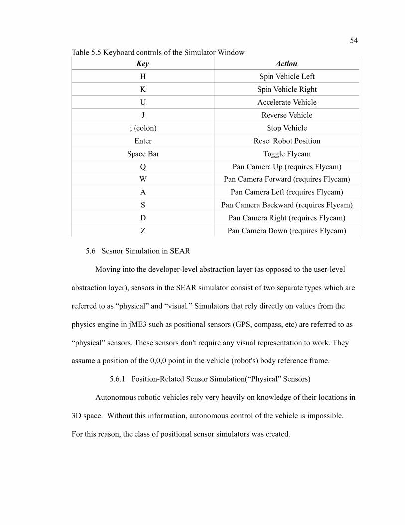
54
Table 5.5 Keyboard controls of the Simulator Window
Key Action
H Spin Vehicle Left
K Spin Vehicle Right
U Accelerate Vehicle
J Reverse Vehicle
; (colon) Stop Vehicle
Enter Reset Robot Position
Space Bar Toggle Flycam
Q Pan Camera Up (requires Flycam)
W Pan Camera Forward (requires Flycam)
A Pan Camera Left (requires Flycam)
S Pan Camera Backward (requires Flycam)
D Pan Camera Right (requires Flycam)
Z Pan Camera Down (requires Flycam)
5.6 Sesnor Simulation in SEAR
Moving into the developer-level abstraction layer (as opposed to the user-level
abstraction layer), sensors in the SEAR simulator consist of two separate types which are
referred to as “physical” and “visual.” Simulators that rely directly on values from the
physics engine in jME3 such as positional sensors (GPS, compass, etc) are referred to as
“physical” sensors. These sensors don't require any visual representation to work. They
assume a position of the 0,0,0 point in the vehicle (robot's) body reference frame.
5.6.1 Position-Related Sensor Simulation(“Physical” Sensors)
Autonomous robotic vehicles rely very heavily on knowledge of their locations in
3D space. Without this information, autonomous control of the vehicle is impossible.
For this reason, the class of positional sensor simulators was created.

55
5.6.1.1 GPS
GPS simulation is not a new concept as shown by Balaguer and Carpin [42].
Though Balaguer and Carpin, as well as Durst and Goodin [94] describe and test
advanced GPS simulation algorithms, it is sufficient to simulate GPS with only basic
functionality. To simplify GPS simulations, satellite tracking is not simulated in SEAR
and as such, no atmospheric anomalies are simulated either. Basic functionality of GPS
is simulated to provide only the latitude, longitude and altitude measurements of the
vehicle's current position. To further simplify the simulation, GPS is simulated as a
roughly flat projection of the terrain. This is similar to the simple version of the
GarminGPS sensor in early Gazebo simulations [95]. Developments will improve or
replace this implementation, but it is important to have a simple and basic version of this
sensor for initial tests of the simulator.
There are several important settings that the user must enter before using the GPS
sensor in a simulation. The first set of values represents the latitude, longitude and
altitude values of the center point of the terrain map being used. These values are then
converted from a string to complete decimal format and will be used as an offset which
helps calculate the updated latitude, longitude and altitude of the robotic vehicle during
simulated movement.
Since the Earth is not a perfect sphere, the length of a longitude degree varies
from 111,320 meters per degree at 0 degrees latitude (the equator) to 0 meters per degree
at 90 degrees latitude (the poles) [96]. Calculating this value on a constant basis can
prove rather costly on computing resources. To simplify the changes in longitudinal
distances, a look up table based on the Zerr's table is used to simulate distance per degree
56
latitude [96]. The value entered by the user of the starting position of the robot vehicle
will be used in this look up table to find the closest matching latitude.
Since it is impractical that a simulation will require a vehicle to travel more than
five latitudinal degrees, the value of the length of a degree is never recalculated during
the simulation.
To find the distance per degree longitude in this simulator, a simple distance
formula (shown in 5.6.1.1.1) is used [97].
Length of a degree of Longitude= Radius of Earth at the Equator×cos ( Latitude)
(5.6.1.1.1)
Distance of a degree of longitude at the equator = 111320.3411 meters as shown
by Zerr. The final formula is shown in Formula (5.6.1.1.2).
Length of one degree of Longitude=111320. 3411 meters×cos ( Latitude)
(5.6.1.1.2)
Since this formula is a fast calculation, it can be calculated each time the GPS
simulator is polled (about 60 times a second) without a large determent to the speed of
the overall simulation.
When the GPS simulator is polled, it finds the distance in three dimensions of the
vehicle from the center of the world space from the current position of the vehicle. These
values are returned in world units and are treated as meters (in this simulator, one world
unit equals one meter). Knowing the offset in three dimensions (in meters) from the
center point of the map as well as the values of the center of the map, the latitude,
longitude, and altitude of the vehicle can be calculated. The current vehicle position on
the X-axis in meters of the vehicle is converted to latitude using the values from Zerr's
table [96]. The latitude of the vehicle is then known and can be used in Formula 5.6.1.1.2

57
to find the length per degree longitude. The current vehicle position in the Z-axis (in
meters) is then divided by this value to find the current longitude of the vehicle. The
current vehicle offset in the Y-axis is added to the value of the altitude of the center of the
terrain map. This gives the actual vehicle altitude in relation to the original center value.
The GPS simulator is accessible through a virtual serial port within MRL. It streams
GPGGA NMEA strings formatted to match the San Jose MTK-3301 GPS receiver series
(specifically the FV-M8) [93].
5.6.1.2 Compass
The compass simulator is single-axis and simple. A Vector3f object is used to
store the position of North. For example, the default location of North is located at x, y, z
ordinates (100000, 0, 0). Since one world unit equals one meter in this simulator, this
means the North Pole is located at 100km on the X-axis of any simulation. Of course, this
value can be changed by the user to a more accurate estimation of actual pole distance
when the latitude and longitude of the terrain are considered. For an accurate calculation,
users can select to enable a magnetic declination calculation. This will use the current
GPS location of the robot to calculate the location of magnetic North relative to the robot.
This calculation uses the NOAA (National Oceanic and Atmospheric Administration)
National Geospatial-Intelligence Agency (NGA) World Magnetic Model (WMM) for the
years of 2010-2015 [98]. The declination is calculated using "GeomagneticField.Java”
from the Android Project [99], [100]. These values are stored in a table and can be
updated by the developer as newer models are released.
The simulator calculates the angle of the robot to north by getting the values of
the forward direction of the robotic vehicle using the getForwardVector() method. The
58
values of this vector of the X and the Z directions represent the forward facing direction
in the X-Z plane. These values are compared to the X and Z values of “North.” The
angle between these two values is the angle between the forward-facing direction of the
robotic vehicle and North. This angle is represented in +/-180 degrees (or +/- PI radians).
When importing terrains from Google Maps, it is important to note that the
location of North in the Google Maps terrain corresponds to the X direction when the
terrain is exported correctly (with North facing upward). This automatically sets North in
the terrain model to the X direction in the simulator when models are loaded from Google
Maps into Sketchup.
The user's code must poll the compass to obtain a current value using code such as
int currentHeading = sear.getCompassResult("comp1") where “comp1” is the compass's
name given by the user. This will return a float value between +/- 180 degrees. The user
can scale and format this data any way they might need to simulate actual hardware. This
sensor doesn't have its own serial port (in many cases in actual hardware as well) so for a
user to communicate with the simulated sensor in the same way as they would with actual
hardware, the user can write a custom controller script which will accept serial
commands, poll the simulator for sensor values, format and scale the data, and return the
data over the virtual serial port.
5.6.1.3 Three-Axis Accelerometer
The use of MEMS (Microelectromechanical Systems) accelerometers is becoming
very common in robotics. Accelerations can be used in dead-reckoning systems as well
as force calculations.
Simulations of accelerations are made simpler because of several methods built

59
into jME3. jME3 provides a getLinearVelocity() method which will return the current
linear velocity of a VehicleControl object in all three dimensions. To get accelerations
from this method, a simple integration of these values over time is taken. To get an
accurate time, the timer class was used. The timer class provides two important methods
used in this integration, getResolution() and getTime(). getResolution() returns the
number of “ticks” per second and getTime() returns the time in “ticks.” These two values
together are used to find time in seconds.
The accelerometer method is called from the physicsTick loop in the simulator
code. This allows it to function continuously during the simulation. The accelerometer
simulator must not take too much time to execute; otherwise it will slow down the entire
simulation. To make sure the main event loop executes quickly, the accelerometer method
does not stall for the given time between measurements, rather it stores a starting time
and calculates the time that has passed every time the main event executes. The elapsed
time is compared to the number of ticks between readings calculated from the bandwidth.
On the first run of a single reading, the first linear velocity is returned from the
getLinearVelocity() method and saved, then the getTime() method saves the current time
(in “ticks”) and a flag is set to prevent this from happening again until the next reading.
Every time the physicsTick() loop runs, it calls the accelerometer method which now
compares the elapsed time from the first reading with the number of ticks between
readings calculated from the bandwidth. When this time has finally elapsed the second
linear velocity is taken and immediately an ending time is saved. The total number of
seconds passed between readings is found by subtracting the number of ticks that have
elapsed during the measurement, and dividing this difference by the resolution of the

60
timer from the getResoultion() method. The acceleration is equal to the second velocity
minus the first velocity divided by the elapsed time in seconds as shown in Formula
5.6.1.3. Once a single reading is finished, the flag for reading the first velocity and
starting time is reset.
(Velocity2−Velocity1)(Elapsed Time in Seconds )
(5.6.1.3)
These readings are for all three axes. Additional error could be simulated by
manipulating these data before it is sent to the user, however, the decision was made not
to handicap the user by forcing them to use a particular error calculation [94]. The user is
free to model high-quality or low-quality accelerometer hardware. The resulting raw
values from all three axes are returned every time the accelerometer is simulated to
simplify coding. If a user is only interested in one axis, the others can be ignored. The
user must poll the accelerometer from their userCode. They first need to start a SEAR
MRL service, then access the simulator from within that service by making a function
call directly to SEAR such as accelerations = sear.getAccelResult("accel") where “accel”
is the name of the sensor given by the user. This sensor does not have its own serial port.
To access the virtual accelerometers in the same way as an actual hardware distance
sensor, a user can write a “custom controller” script which accepts serial messages, polls
the simulator for sensor values, formats and scales the data, then returns the data over the
virtual serial port.
5.6.1.4 Three-Axis Gyroscope
Gyroscopes often accompany accelerometers in the design of inertial measuring
systems. They can be used to help correct offsets and errors given by real-world
accelerometers. There is no error in the simulated accelerometers in this simulator, but

61
the results are often “jittery” due to the way the physics engine simulates both
accelerating and braking of the vehicle. Users may still want to use the gyroscope in the
standard way to improve their filtering algorithms. Real-world MEMS gyroscopes often
have a large output drift. This drift isn't currently simulated.
jME3 has a method to return angular velocity, however, it does not return values
in radians per second. In fact, it could not be determined exactly what units it returned
even with the help of the developer's forum. A custom method for finding actual angular
velocity was created that is very similar to the accelerometer simulator.
Again, jME's timer class was used to find timer resolution (in “ticks” per second)
and elapsed time, in ticks. To find the angle traveled over an elapsed time, the
getForwardVector() method was used. This method returns the 3D normal vector of the
forward direction of the VehicleControl object. For the first run of a sensor reading, the
first forward direction vector and start time are recorded then a flag is set to prevent this
from happening again until the next reading. The current time is compared with the
expected elapsed time until it is reached. At this point the second forward direction
vector is recorded as well as the stop time. Since the Vector3f class has no methods for
comparing the angle between the components, both of the forward vectors are projected
on each of the three original planes; XY, YZ and XZ. Each of these values are stored in a
Vector2f. Using the angleBetween() method in the Vector2f class, the angle between
each projected portion of the forward directions are calculated. For example, XY1 are
the X and Y components of the first forward vector and XY2 are the X and Y components
of the second forward vector. XY1.angleBetween(XY2) returns the angle between these
components. This would describe a rotation about the Z-axis (yaw). Once the angle

62
traveled in each axis is found the elapsed time is used to find the angular velocity. The
angular velocity is then returned to the user. As with the accelerometer, all three axes are
always simulated regardless of how many axes the user is measuring and the resulting
values are without error. The user can choose to model error for any particular gyroscope
they plan to use. A very good scheme for modeling error for a MEMS gyroscope can be
found in [94].
To access the gyroscope readings, a user must follow the same method as with the
accelerometer. (I.e. start a SEAR service within MRL, then poll the simulator for the gyro
values). The function call would be GyroReadings = sear.getGyroResult("gyroscope")
where “gyroscope” is the name of the sensor given by the user. This sensor does not have
its own serial port. To access the virtual distance sensor in the same fashion as an actual
hardware gyroscope sensor, a user can write a “custom controller” script which accepts
serial messages, polls the simulator for sensor values, formats and scales the data, then
returns the data over the virtual serial port.
5.6.1.5 Odometer
Odometry is a very useful metric used in positioning calculations for vehicles.
The odometer sensor tracks the distance the robot has moved in both the forward and
reverse directions. As with the other “physical” sensors, the odometer assumes it is
located at the center of the robot's body. There is a minimum threshold that must be met
in any linear direction before distances will be logged. This is due to the way jBullet
simulates vehicle objects. When the robot (a type of vehicle object) is stopped, the brakes
are constantly “fighting” with the acceleration setting, causing the vehicle to shake ever
so slightly. Without the threshold value mentioned above, these vibrations would accrue

63
to a very large error in odometer readings over time.
The way users can access this sensor is different from any of the others because
the odometer sensor is a component of a “robot” object by default in SEAR. This means
that a user can measure this sensor by sending a message to the robot object's virtual
serial port in Roomba protocol format. SEAR will return the data on the virtual serial
port in the same format as an actual Roomba would. Like an actual Roomba, SEAR
stores the value of the distance as a 16-bit signed value (between -32,768 and +32,767)
and sends the data as high-byte then low-byte when it is requested. Once the value has
been requested by the user it is reset to 0, again, the same as with an actual Roomba [84].
5.6.2 Reflective Beam Simulation (“Visual” Sensors)
Beam reflection sensors are arguably the most common sensors used in robotics.
This sensor class includes sensors such as Infrared (IR), RADAR, SONAR, LIDAR, and
Ultrasonic sensors. Though the technologies behind these types of sensor differ, they
operate on the same principles. In the real world, this type of sensor works by sending a
signal out into the environment and measuring the time it takes for that signal to reflect
back to the sensor. SEAR uses ray casting to simulate this class of sensors. The reason
these sensors are referred to as “visual” sensors in this dissertation is that the rays are cast
along graphical lines drawn in the environment. These lines help users determine exactly
what objects are being detected by the simulated sensors. Many simulators use ray
casting as a method for finding intersections with triangle meshes of objects in a virtual
environment [101].
5.6.2.1 Ultrasonic, Infrared, RADAR and SONAR Distance Sensors
The distance sensor class is used to simulate reflective sensors such as ultrasonic,

64
infrared, RADAR and SONAR. The concept of these sensors is simple, though their
implementation is quite complicated. To match specific sensors, actual hardware was
designed and tested at specific distances and spread angles. Currently a “PING)))”
ultrasonic sensor is the only one that has been validated against actual hardware
measurements in this way. Distance sensors are implemented by having nested cone-
shaped arrays of graphical lines. This group of lines may be attached at any given point
on the robot, and rotated to point in any direction [64], [102], [103].
Each nested cone of lines has a slightly different angle from the X-axis of the ray's
reference frame. Each nested cone also has a different length and color. The angles and
length correspond better to the actual lobes of the ultrasonic sensor. The number of lines
in each particular cone and the total number of cones define the sensor's resolution.
During simulation, a list of “distance sensor” objects is used to iteratively cast rays along
each line of each sensor. For a given sensor, only the closest collision distance and
collision point can be returned. The collision point is used to display a red sphere at the
actual point of impact on whatever object the sensor happens to detect. This helps the
user debug their robotics projects by visually representing the point that is being detected
by the sensor. If no objects are detected within range of the sensor, then the maximum
sensing distance is returned by the sensor.

65
(a) (b) (c) Figure 5.6.2.1.1 The distance sensor beam pattern is adjustable in SEAR. (a) Shows the
beam pattern of a PING))) brand sensor which was experimentally acquired. (b) Shows an example of an infrared sensor beam. (c) Shows an example of the side lobes of the beam pattern being simulated
The angles, ranges, and resolution of the sensors are adjustable by end users (as
well as developers) of SEAR as shown in Figure 5.6.2.1.1 and 5.6.2.1.2. This allows for a
wide range of sensors and sensor types to be simulated by this particular simulator. IR
and Ultrasonic beams can have a variety of different shapes depending on the
applications they are used for. Sensors in the Sharp family of IR sensors generally have
an ovate or “football” shape. They have much more narrow beams and are less prone to
errors due to collision with angled objects while the MaxBotix EZ series ultrasonic
sensors have more of a teardrop beam pattern [104]–[106]. All of this can be simulated
as long as the developer knows the particular beam pattern of the sensor to be simulated.
It is recommended to measure these values experimentally since datasheets often use
different methods for determining values listed in the given charts and graphs which may
not be useful for the particular environment in which the sensor will be used. The nested
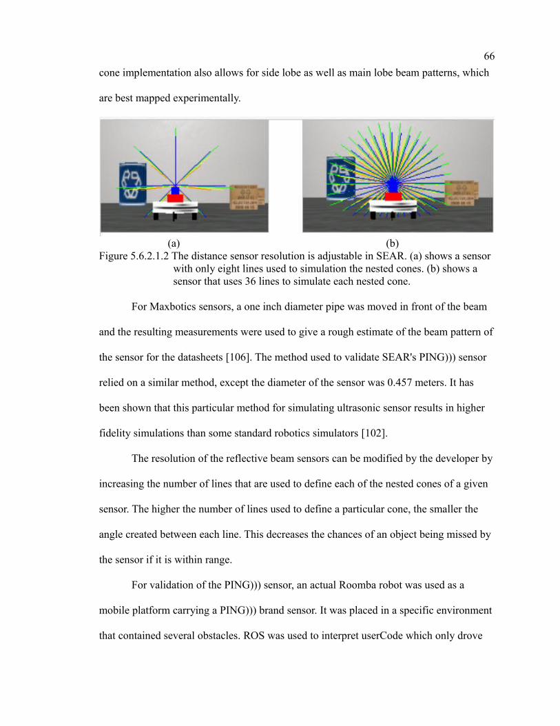
66
cone implementation also allows for side lobe as well as main lobe beam patterns, which
are best mapped experimentally.
(a) (b) Figure 5.6.2.1.2 The distance sensor resolution is adjustable in SEAR. (a) shows a sensor
with only eight lines used to simulation the nested cones. (b) shows a sensor that uses 36 lines to simulate each nested cone.
For Maxbotics sensors, a one inch diameter pipe was moved in front of the beam
and the resulting measurements were used to give a rough estimate of the beam pattern of
the sensor for the datasheets [106]. The method used to validate SEAR's PING))) sensor
relied on a similar method, except the diameter of the sensor was 0.457 meters. It has
been shown that this particular method for simulating ultrasonic sensor results in higher
fidelity simulations than some standard robotics simulators [102].
The resolution of the reflective beam sensors can be modified by the developer by
increasing the number of lines that are used to define each of the nested cones of a given
sensor. The higher the number of lines used to define a particular cone, the smaller the
angle created between each line. This decreases the chances of an object being missed by
the sensor if it is within range.
For validation of the PING))) sensor, an actual Roomba robot was used as a
mobile platform carrying a PING))) brand sensor. It was placed in a specific environment
that contained several obstacles. ROS was used to interpret userCode which only drove

67
the Roomba forward at a specified speed and recorded values from the Roomba's
odometer and the PING))) to a file. The test robot and its validation test results can be
seen in Figure 5.6.2.1.3.
(a) (b) Figure 5.6.2.1.3 (a) The actual Roomba robot with ultrasonic sensor payload on top. (b)
The resulting graph of the odometer reading versus the Ultrasonic reading as the robot drove through the test environment.
The same environment was designed for the ROSStage simulator. A similar robot
was designed for the simulator and the exact same code was tested. The resulting
odometer and ultrasonic sensor values were saved to a file. It should be noted that Stage
does not simulate the correct beam-pattern of the sensor, rather it only simulates a section
of a circle. The Stage simulation and its test results can be seen in Figure 5.6.2.1.4.
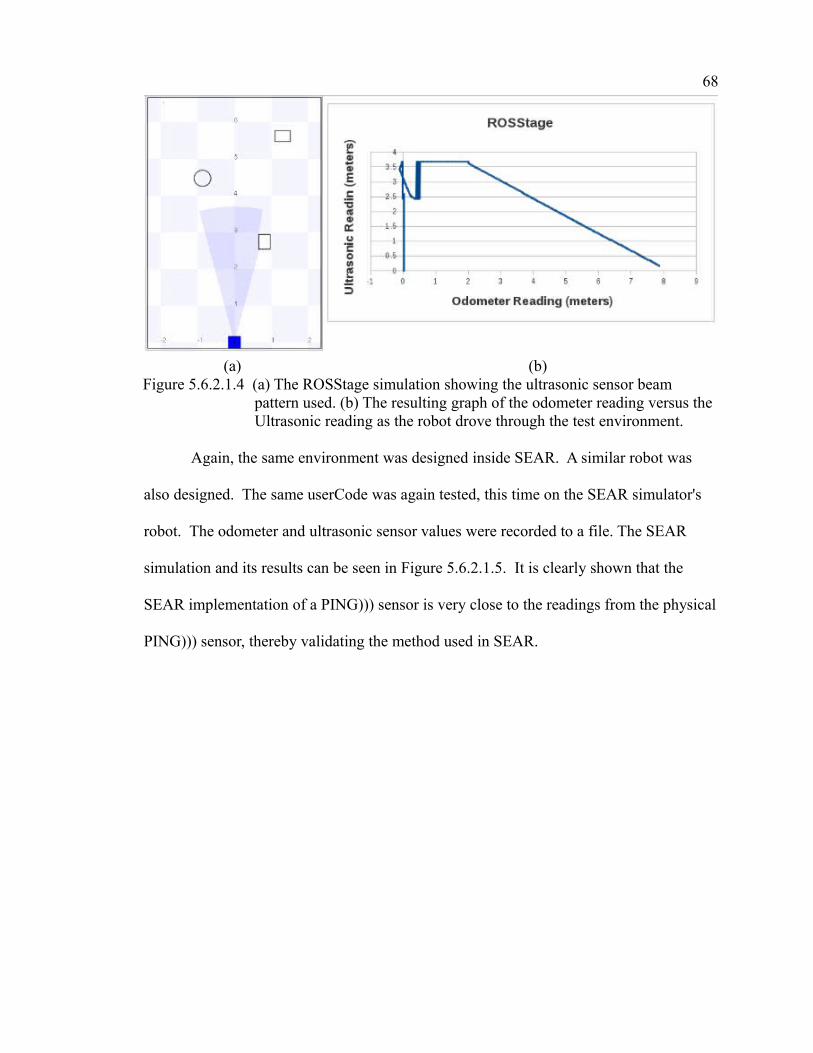
68
(a) (b) Figure 5.6.2.1.4 (a) The ROSStage simulation showing the ultrasonic sensor beam
pattern used. (b) The resulting graph of the odometer reading versus the Ultrasonic reading as the robot drove through the test environment.
Again, the same environment was designed inside SEAR. A similar robot was
also designed. The same userCode was again tested, this time on the SEAR simulator's
robot. The odometer and ultrasonic sensor values were recorded to a file. The SEAR
simulation and its results can be seen in Figure 5.6.2.1.5. It is clearly shown that the
SEAR implementation of a PING))) sensor is very close to the readings from the physical
PING))) sensor, thereby validating the method used in SEAR.

69
(a) (b)Figure 5.6.2.1.5 (a) The SEAR Roomba simulation showing the ultrasonic sensor beam
pattern used. (b) The resulting graph of the odometer reading versus the Ultrasonic reading as the robot drove through the test environment.
The user can attach multiple distance sensors to their robot any at attachment
point they choose and orient the sensors in any way they choose (Figure 5.6.2.1.6 shows
an example of this). Each sensor must have a custom name so SEAR will know from
which one to acquire data. To interface with these sensors in SEAR, the user must first
start an instance of a SEARservice, then make a function call to the simulator from the
SEARservice. The user must pass to the function the name of the sensor they wish to
poll such as distance = sear.getDistanceResult("Ping1") where Ping1 is the name the user
gave the sensor when creating the robot. The resulting value is returned in meters. The
user can scale and format this as needed. This sensor does not have its own serial port. To
access the virtual distance sensor in the same way as an actual hardware distance sensor,
a user can write a “custom controller” script which accepts serial messages, polls the
simulator for sensor values, formats and scales the data, then returns the data over the
virtual serial port.
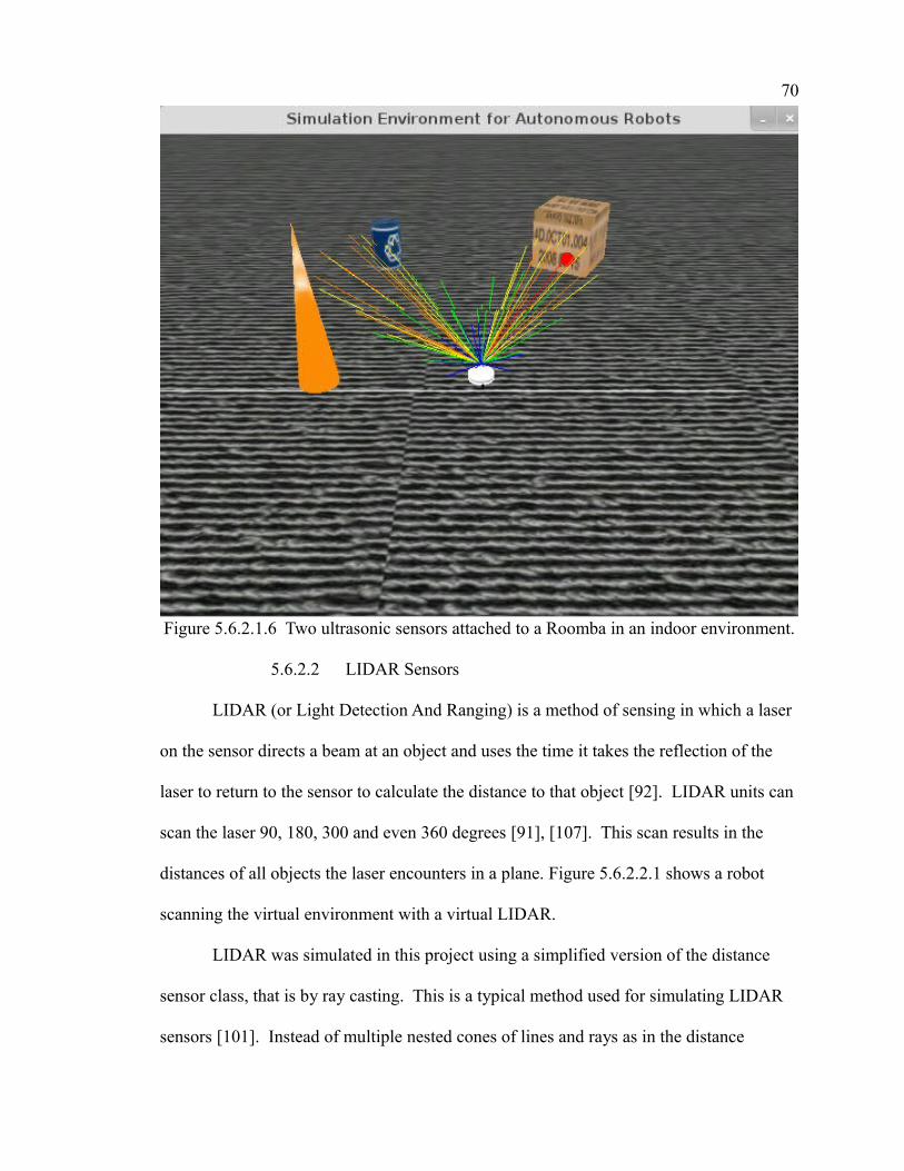
70
Figure 5.6.2.1.6 Two ultrasonic sensors attached to a Roomba in an indoor environment.
5.6.2.2 LIDAR Sensors
LIDAR (or Light Detection And Ranging) is a method of sensing in which a laser
on the sensor directs a beam at an object and uses the time it takes the reflection of the
laser to return to the sensor to calculate the distance to that object [92]. LIDAR units can
scan the laser 90, 180, 300 and even 360 degrees [91], [107]. This scan results in the
distances of all objects the laser encounters in a plane. Figure 5.6.2.2.1 shows a robot
scanning the virtual environment with a virtual LIDAR.
LIDAR was simulated in this project using a simplified version of the distance
sensor class, that is by ray casting. This is a typical method used for simulating LIDAR
sensors [101]. Instead of multiple nested cones of lines and rays as in the distance

71
sensors, a single flat plane of graphical lines are drawn on the screen originating from the
location of the sensor (as given by the user). The lines have a length equal to the
maximum range of the LIDAR sensor. The length of the visual line determines the
maximum range of the ray cast along that line. This value is given in the LIDAR's
datasheet and can be set by the user.
Figure 5.6.2.2.1 A single scan from the LIDAR simulator on a test environment. The red lines show where the rays are cast and the yellow spheres
shows where the rays collide with the box objects. The results of this simulation can be seen in Figure 5.6.2.2.2b
Inside the SEAR simulator itself, the SICK LMS200 LIDAR was modeled and
simulated. The sensor interfaces through a virtualSearialPort object within MRL and is
accessible from userCode in the same way as actual hardware. This requires the user to
start a LIDAR service within MRL, and passing it the path of the virtualSerialPort object

72
as the port for the service to connect. Figure 5.6.2.2.2 shows a comparison of an actual
SICK LMS200 scan of the lab environment versus a scan of the equivalent environment
in the simulator (the environment shown in Figure 5.6.2.2.1). The major differences that
can be seen between the two scans are mainly due to the fact that the simulated LIDAR
does not calculate the scattering or absorption of the laser beam once it hits an object.
Otherwise it is very easy to identify the edges and sides of the boxes that were scanned.

73
Figure 5.6.2.2.2 (a) The readings from an actual SICK LMS200 (b) the readings from
the SEAR simulated LIDAR in a similar environment. These readingsprovide a top-down view of an environment in which there are two larger boxes at the left and right extremes and two smaller boxes in the front center of a wall in front of the LIDAR sensor.

74
The algorithm for simulating the scan involves finding the current 3D translation
and rotation of the LIDAR sensor. The sensor is placed on the robot's body by the user
when designing the robot. As the robot moves within the world, the position of the
LIDAR sensor updates. The graphical lines of the LIDAR are updated automatically
(since they are part of the robot's Node object). During the physicTick() loop, in which all
of the physics are calculated in jME, rays are cast along each graphical line. The resulting
collision points with any other object in the physics space are returned. If no collision is
detected within the distance of the maximum range, then the value of the maximum range
is returned. The simulation results are a set of distances. Each distance corresponds to a
particular line.
An example scan with a maximum degree spread equal to 180 degrees and an
angle step of 0.5 degrees per step would include 361 readings; one each at the following
angles:
0º, 0.5º, 1º, 1.5º, 2º ... 178º, 178.5º, 179º, 179.5º, 180º
The result of the measurements is an array of floating point decimal numbers
representing distances to collisions in world-units. Just as with actual LIDAR systems,
this information is packaged with a header and checksum value. Figure 5.6.2.2.2 shows
two examples of LIDAR sensors with different properties.
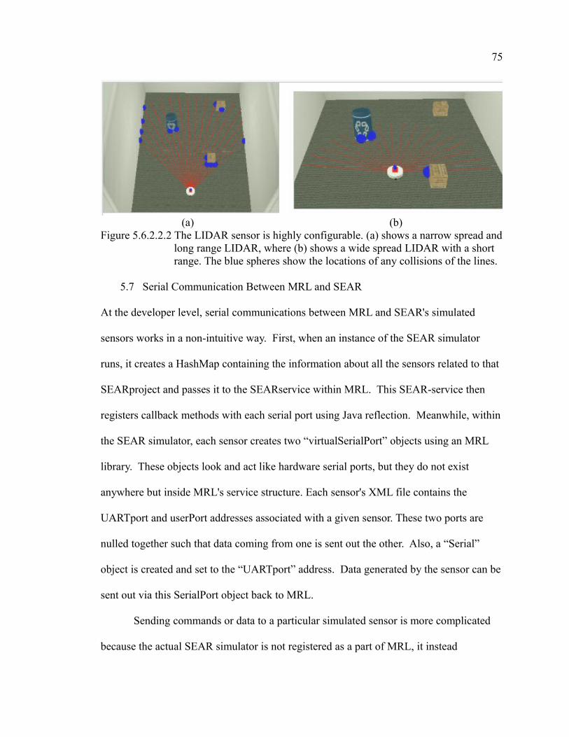
75
(a) (b) Figure 5.6.2.2.2 The LIDAR sensor is highly configurable. (a) shows a narrow spread and
long range LIDAR, where (b) shows a wide spread LIDAR with a short range. The blue spheres show the locations of any collisions of the lines.
5.7 Serial Communication Between MRL and SEAR
At the developer level, serial communications between MRL and SEAR's simulated
sensors works in a non-intuitive way. First, when an instance of the SEAR simulator
runs, it creates a HashMap containing the information about all the sensors related to that
SEARproject and passes it to the SEARservice within MRL. This SEAR-service then
registers callback methods with each serial port using Java reflection. Meanwhile, within
the SEAR simulator, each sensor creates two “virtualSerialPort” objects using an MRL
library. These objects look and act like hardware serial ports, but they do not exist
anywhere but inside MRL's service structure. Each sensor's XML file contains the
UARTport and userPort addresses associated with a given sensor. These two ports are
nulled together such that data coming from one is sent out the other. Also, a “Serial”
object is created and set to the “UARTport” address. Data generated by the sensor can be
sent out via this SerialPort object back to MRL.
Sending commands or data to a particular simulated sensor is more complicated
because the actual SEAR simulator is not registered as a part of MRL, it instead

76
communicates to MRL via the SEARservice. When data is sent from userCode to a
particular SEAR virtual sensor, it cannot travel directly on the sensor's serial port service
like data coming the other direction. Instead, it triggers a set of events within the MRL
SEARservice. First, the type of sensor is acquired by looking at the message being sent.
Then everything except the sensor's name is stripped from the message. For instance:
"myLidar_LIDARsimulator_Serial_Service" becomes "myLidar". Once the sensor's type
and name are known, the SEARservice can then send the userData to that instance of the
sensor. Figure 5.7 shows a graphical representation of the dataflow when userCode sends
a message to a LIDAR to acquire data, and how that sensor sends data back to the
userCode. The steps described in the figure are:
1. User code running within a python service sends a message to the LIDAR serial service requesting a scan (this is the same as with actual hardware).
2. The LIDAR service sends the serial data to the LIDAR simulator's serial port, but the message is processed by the SEARservice.
3. The SEARservice invokes the particular LIDAR simulator instance within the SEAR simulator.
4. The SEAR simulator makes a method call to the particular LIDAR simulator instance.
5. The LIDAR scans the simulated environment, formats the data and sends it to its Serial service.
6. The LIDAR's serial service sends the data back to the LIDAR service.
7. The LIDAR service sends the data to the userCode running within the Python service.

77
Figure 5.7 The data flow diagram of serial messages between userCode in MRL's Pythonservice and SEAR simulated sensors.
All of this action occurs to abstract the userCode so users will interface with the
simulated LIDAR the same way they would as with an actual LIDAR, by a method call
in the LIDARservice. To the user, all of these other communications are hidden. The
only difference the user will notice is the serial port name of the simulated LIDAR
doesn't appear anywhere outside of MRL. If they check the device manger in windows or
run a directory listing in /dev/ on UNIX or LINUX-based machines, the serial port will
not be listed.

CHAPTER 6: CONCLUSIONS AND FURTHER WORK
This research developed the methods and techniques for the design of a tool that
can be used for a variety of academic uses, from teaching introductory programming
concepts to performing accurate graduate-level robotics research. This design was
demonstrated by the development of the Simulation Environment for Autonomous
Robots. Most of the accomplishments planned for this research have been met. These
include the following:
Identification of features and a working architecture for a modern robotics
simulator:
As defined in this work, a modern robotics simulator, SEAR, is available
to users on any major platform (Windows, Mac and Linux). It also is open source
meaning the source code is freely distributed, allowing a community of
developers can improve it over time. One of the most important aspects of a
successful modern robotics simulator is the ability to interface with at least one of
the many middleware applications that are currently available. This greatly
increases the usability of the simulator and extends the capability of the user by
allowing them to use third-party libraries and software easily.
The creation of methods for simulating different types of sensors in a virtual 3D
environment:
Common sensors (a 3D accelerometer, a 3D gyroscope, a magnetic
compass, an odometer, a GPS, a LIDAR, and a class of reflective distance sensors

79
including ultrasonic and infrared) used in autonomous robotics projects have been
developed and several have been validated against actual hardware. The method
of simulation of some of these sensors is novel. For example, the distance sensors
are simulated in such a way that beam patterns of these sensors can be adjusted by
the user.
The addition of new sensor types to SEAR and improvement of current sensors:
The odometer sensor was added to keep track of the overall distance the
robotic vehicle traverses. Also, the new class of “visual” sensors which includes
Ultrasonic, SONAR, RADAR and infrared sensors as well as a user-definable
LIDAR sensor were added.
Users can define custom beam shapes for the distance sensor class such
that they can include all makes and models of sensors of this class. The compass
sensor class was made more efficient by the addition of a new declination
calculation method.
Implementation of an interface with common robotics middleware:
The same user-defined code can be used on actual hardware or the SEAR
simulator with little to no modification.
The implementation of a method for users to import or create models:
Custom terrains can now be designed by the user using SEAR's POJO
library. Models of terrains can also be imported from external CAD software. The
resulting terrains and obstacles are saved as XML files that are dynamically
injected into SEAR at start up. These files can be created and manipulated by
hand if needed and transferred from one user to another easily.

80
Robots can be built component by component using the SEAR POJO
library. Components of robots can be imported from external CAD software. The
suspension characteristics of the robot are completely accessible to the user
including mass, damping, compression, wheel rest length, stiffness and maximum
suspension force.
The implementation of a simple file extension for SEAR projects:
Settings of entire SEARprojects are stored as a single zip file which
contains all the user's code, models, and files for robots and terrains.
6.1 Virtual Serial Ports and ROS Integration
All of the goals set for this research were met or exceeded with the exception of
interfacing with ROS middleware using virtual serial ports. Previous iterations of SEAR
had interfaced with ROS directly (as it now does with MRL). This proved hazardous for
development as the infrastructure of ROS changed multiple times, completely
invalidating the deprecated method used. The most effective way to interface with ROS
was determined to be at the highest abstraction level, away from the internal changes
within the ROS project. For SEAR, it was determined that only serial communication to
specific ROSnodes (such as the Brown University Roomba driver, or the Arduino serial
driver) would protect SEAR from the constant code revisions. The method for
connecting two serial was to use pseudoterminals as virtual serial ports. This method was
expected to provide a relatively clean connection between ROS and SEAR, while
keeping one of the main concepts of SEAR intact; interfacing with SEAR simulated
hardware should be the same as interfacing with actual hardware. The pseudoterminals
are configured in such a way to pass inputs from one pseudoterminal to the output of the

81
other and vice versa. If this method had worked, a single implementation of SEAR could
be used to communicate with both MRL and ROS.
Through many investigations, if was determined that the use of pseudoterminals
does not work for piping ROS data through to MRL and subsequently SEAR. By adding
a secondary hardware serial port in parallel with the an actual Roomba connected to
ROS, it was shown that ROS sends different commands to an actual Roomba than it
sends when connected to a pseudoterminal. This makes it impossible to implement a
serial interface with ROS using the ROS Roomba node via pseudoterminals.
There are two possible solutions to this, and neither of which were determined to
be suitable for the needs of most users. The first method requires nulling together two
actual serial ports on the host machine that ROS and SEAR are running on. This is a
physical implementation of how the pseudoterminals work.
The second way to allow ROS to communicate to MRL, and thereafter SEAR,
would be to use a package called ROSbridge that converts ROS commands to TCP
protocol. This would require MRL to implement a TCP protocol as well which does not
conform to the goals set out in this research; to interface with SEAR exactly the same
way as with actual hardware. As such, this method was not investigated any further.
6.2 Further Work
There are many opportunities for improvement of the SEAR simulator. Additional
sensor types could extend the capability of SEAR. Some good candidates for new sensors
include visual cameras, infrared cameras, and 3D depth cameras (such as an XBOX
kinect). More models of the currently supported sensors could be added as well. For
instance the GPS and LIDAR simulators are each based on only one actual sensor brand

82
and model respectively. The addition of new beam shapes for the infrared is also
possible, though this ability is already available to the end user as they can use one of the
overloaded constructors in the POJOs library to define their own beam shapes. It would
be simple to add in different beam shapes based on names so that when a user names a
sensor “MaxBotics EZ1” SEAR will automatically use the beam pattern built in to
simulator that particular sensor.
Moving each sensor simulation into their own threads would also increase the
ability of SEAR by reducing lag time when large amounts of data are being collected.
Each sensor could be encapsulated in its own thread. This would also allow for an
expansion of SEAR from simulating a single robot, to the ability to simulate multiple
robots. Since there is a large amount of graduate-level research in these areas this ability
would increase the usage of SEAR.

83
REFERENCES
[1] T. Bräunl, “The Eyesim Mobile Robot Simulator,” 2000.
[2] T. Bräunl and A. Koestler, “Mobile Robot Simulation with Realistic Error Models,” inInternational Conference on Autonomous Robots and Agents, 2004, vol. 51, no. 6, pp. 46–51.
[3] T. Machado, M. Sousa, S. Monteiro, and E. Bicho, “CoopDynSim: a 3D robotics simulator,” pp. 45–50, 2012.
[4] R. Pjesivac, “Gazebo Tutorial.”
[5] J. Craighead, J. Burke, and R. Murphy, “SARGE: A User-centric Robot Simulator andTraining Environment,” in International Conference on Human-Robot Interaction,Amsterdam, 2008.
[6] “CogNation • View topic - Create model with Google Sketchup.” [Online]. Available: http://cogmation.com/forum/viewtopic.php?f=9&t=6.
[7] B. P. Gerkey, R. T. Vaughan, and A. Howard, “The Player / Stage Project : Tools for Multi-Robot and Distributed Sensor Systems,” in The International Conference onAdvanced Robotics, 2003, no. Icar, pp. 317–323.
[8] J. Craighead, R. Gutierrez, J. Burke, and R. Murphy, “Validating the Search and Rescue Game Environment as a robot simulator by performing a simulated anomaly detection task,” in 2008 IEEE/RSJ International Conference on Intelligent Robots and Systems, 2008, pp. 2289–2295.
[9] S. Carpin, M. Lewis, J. Wang, S. Balakirsky, and C. Scrapper, “Bridging the gap between simulation and reality in urban search and rescue.”
[10] T. Laue, K. Spiess, T. Rofer, and T. R, “SimRobot – A General Physical Robot Simulator and Its Application in RoboCup,” in RoboCup 2005: Robot Soccer World Cup IX, Springer Berlin / Heidelberg, 2006, pp. 173–183.
[11] M. Quigley, B. Gerkey, K. Conley, J. Faust, T. Foote, J. Leibs, E. Berger, R. Wheeler,and A. Ng, “ROS : an Open-Source Robot Operating System,” in ICRA Workshop on Open Source Software, 2009, no. Figure 1.
[12] Cyberbotics Ltd., “Webots User Guide release 6.3.3.” 2010.
[13] O. Michel, “Cyberbotics Ltd. Webots TM : Professional Mobile Robot Simulation,” Int. J. Adv. Robot. Syst., vol. 1, no. 1, pp. 39–42, 2004.
84
[14] “Microsoft Robotics.” [Online]. Available: http://msdn.microsoft.com/en-us/robotics.
[15] J. Craighead, R. Murphy, J. Burke, and B. Goldiez, “A Survey of Commercial & Open Source Unmanned Vehicle Simulators,” in Proceedings 2007 IEEE International Conference on Robotics and Automation, 2007, no. April, pp. 852–857.
[16] R. Mendonca, P. Santana, F. Marques, A. Lourenco, J. Silva, and J. Barata, “Kelpie: A ROS-Based Multi-robot Simulator for Water Surface and Aerial Vehicles,” 2013IEEE Int. Conf. Syst. Man, Cybern., pp. 3645–3650, Oct. 2013.
[17] A. Nagaty, S. Saeedi, C. Thibault, M. Seto, and H. Li, “Control and Navigation Framework for Quadrotor Helicopters,” J. Intell. Robot. Syst., vol. 70, no. 1–4, pp. 1–12, Oct. 2012.
[18] Z. Kootbally, S. Balakirsky, and A. Visser, “Enabling codesharing in Rescue Simulation with USARSim / ROS,” in Proceedings of the 17th RoboCup Symposium, 2013.
[19] S. Balakirsky and Z. Kootbally, “USARSim/ROS: A Combined Framework for Robotic Control and Simulation,” in ASME/ISCIE 2012 International Symposium on Flexible Automation, 2012, p. 101.
[20] A. Elkady and T. Sobh, “Robotics Middleware: A Comprehensive Literature Survey and Attribute-Based Bibliography,” J. Robot., vol. 2012, pp. 1–15, 2012.
[21] P. Castillo-Pizarro, T. V. Arredondo, and M. Torres-Torriti, “Introductory Survey to Open-Source Mobile Robot Simulation Software,” 2010 Lat. Am. Robot. Symp. Intell. Robot. Meet., pp. 150–155, Oct. 2010.
[22] C. Madden, “An Evaluation of Potential Operating Systems for Autonomous Underwater Vehicles.” DSTO Defence Science and Technology Organisation, 2013.
[23] A. C. Harris and J. M. Conrad, “Survey of popular robotics simulators, frameworks, and toolkits,” in Proceedings of IEEE SoutheastCon, 2011, pp. 243–249.
[24] “Player Project.” [Online]. Available: http://playerstage.sourceforge.net/.
[25] B. P. Gerkey, R. T. Vaughan, M. J. Matari, A. Howard, K. Stoy, G. S. Sukhatme, and M. J. Mataric, “Most valuable player: a robot device server for distributed control,” in Proceedings 2001 IEEE/RSJ International Conference on Intelligent Robots and Systems. Expanding the Societal Role of Robotics in the Next Millennium (Cat. No.01CH37180), 2001, no. Iros, pp. 1226–1231.
85
[26] N. Bredeche, J.-M. Montanier, B. Weel, and E. Haasdijk, “Roborobo ! a Fast Robot Simulator for Swarm and Collective Robotics,” no. Ppsn, p. 2, Apr. 2013.
[27] R. T. Vaughan, A. Howard, and B. Gerkey, “On Device Abstractions for Portable, Reusable Robot Code,” in IEEE/RSJ International Conference on Intelligent Robots and Systems (IROS), 2003, no. October, pp. 2421–2427.
[28] “Basic FAQ - Playerstage.” [Online]. Available: http://playerstage.sourceforge.net/wiki/Basic_FAQ
[29] “Player Project: Gazebo.” [Online]. Available: http://playerstage.sourceforge.net/index.php?src=gazebo
[30] M. E. Dolha, “3D Simulation in ROS Outline (slides),” Simulation, Nov-2010. [Online]. Available: http://www.ros.org/wiki/Events/CoTeSys-ROS-School?action=AttachFile&do=get&target=3d_sim.pdf [Accessed: 01-Dec-2010].
[31] “Usarsim.” [Online]. Available: http://usarsim.sourceforge.net/wiki/index.php/Main_Page [Accessed: 14-Nov-2010].
[32] G. Roberts, S. Balakirsky, and S. Foufou, “3D Reconstruction of Rough Terrain for USARSim using a Height-map Method,” Proc. 8th Work. Perform. Metrics Intell. Syst. - Permis ’08, p. 259, 2008.
[33] B. Balaguer, S. Balakirsky, S. Carpin, M. Lewis, and C. Scrapper, “USARSim: A Validated Simulator for Research in Robotics and Automation,” in Workshop on “Robot Simulators: Available Software, Scientific Applications and Future Trends”, at IEEE/RSJ IROS 2008.
[34] S. Okamoto, K. Kurose, S. Saga, K. Ohno, and S. Tadokoro, “Validation of Simulated Robots with Realistically Modeled Dimensions and Mass in USARSim,” in IEEE International Workshop on Safety, Security and Rescue Robotics (SSRR), 2008, pp. 77–82.
[35] S. Carpin, M. Lewis, J. Wang, S. Balakirsky, and C. Scrapper, “USARSim: A Robot Simulator for Research and Education,” Proc. 2007 IEEE Int. Conf. Robot. Autom.,pp. 1400–1405, Apr. 2007.
[36] “4. Installation - Usarsim.” [Online]. Available: http://usarsim.sourceforge.net/wiki/index.php/4._Installation
[37] “SourceForge.net: Topic: Confused about installing USARSim on Linux.” [Online]. Available: http://sourceforge.net/projects/usarsim/forums/forum/486389/topic/3873619

86
[38] S. Carpin, T. Stoyanov, Y. Nevatia, M. Lewis, and J. Wang, “Quantitative Assessments of USARSim Accuracy,” Perform. Metrics Intell. Syst., 2006.
[39] S. Carpin, J. Wang, M. Lewis, A. Birk, and A. Jacoff, “High Fidelity Tools for Rescue Robotics : Results and Perspectives,” in Robocup 2005: Robot Soccer World Cup IX, Springer, 2006, pp. 301–311.
[40] M. Zaratti, M. Fratarcangeli, and L. Iocchi, “A 3D Simulator of Multiple Legged Robots based on USARSim,” in Robocup 2006: Robot Soccer World Cup, Springer, 2007, pp. 13–24.
[41] C. Pepper, S. Balakirsky, and C. Scrapper, “Robot simulation physics validation,” in Proceedings of the 2007 Workshop on Performance Metrics for Intelligent Systems- PerMIS ’07, 2007, pp. 97–104.
[42] B. Balaguer and S. Carpin, “Where Am I ? A Simulated GPS Sensor for Outdoor Robotic Applications,” in Simulation, Modeling, and Programming for Autonomous Robots, Springer Berlin / Heidelberg, 2008, pp. 222–233.
[43] A. Birk, J. Poppinga, T. Stoyanov, and Y. Nevatia, “Planetary Exploration in USARsim : A Case Study including Real World Data from Mars,” in RoboCup 2008: Robot Soccer World Cup XII, no. figure 1, Springer Berlin / Heidelberg, 2009, pp. 463–472.
[44] “SARGE.” [Online]. Available: http://www.sargegames.com/page1/page1.html [Accessed: 02-Nov-2010].
[45] J. Craighead, J. Burke, and R. Murphy, “Using the Unity Game Engine to Develop SARGE : A Case Study,” in Simulation Workshop at the International Conference on Intelligent Robots and Systems (IROS), 2008.
[46] I.T. Pier, “SARGE User Manual Search and Rescue Game Environment,” Compass, 2008.
[47] “Carnegie Mellon UberSim Project.” [Online]. Available: http://www.cs.cmu.edu/~robosoccer/ubersim/
[48] “Downloads.” [Online]. Available: http://www.cs.cmu.edu/~coral/download/. [Accessed: 14-Dec-2010].
[49] B. Browning and E. Tryzelaar, “ÜberSim ubersim : A Multi-Robot Simulator for Robot Soccer (Long Version),” Manager, 2000.
[50] A. Waggershauser and A. G. . und Prozessrechentechnik, “Simulation of Small Autonomous Mobile Robots,” University of Kaiserslautern, 2002.
87
[51] “SubSim.” [Online]. Available: http://robotics.ee.uwa.edu.au/auv/subsim.html [Accessed: 05-Dec-2010].
[52] T. Bielohlawek, “SubSim - An Autonomous Underwater Vehicle Simulation System,” 2006.
[53] “OpenRAVE.” [Online]. Available: http://openrave.programmingvision.com/index.php/Main_Page [Accessed: 12-Dec-2010].
[54] R. Diankov and J. Kuffner, “Openrave: A planning architecture for autonomous robotics,” Robot. Institute, Pittsburgh, PA, Tech. Rep. C., no. July, 2008.
[55] “OpenRAVE and ROS | Willow Garage.” [Online]. Available: http://www.willowgarage.com/blog/2009/01/21/openrave-and-ros
[56] “The Mobile Robot Programming Toolkit.” [Online]. Available: http://www.mrpt.org/
[57] M. Perception, “MRPT Book -- Development of Scientific Applications with the Mobile Robot Programming Toolkit,” October, 2010.
[58] J. L. . Claraco, “Development of Scientific Applications with the Mobile Robot Programming Toolkit: The MRPT reference book,” Univ. Malaga, 2010.
[59] “About MRPT | The Mobile Robot Programming Toolkit.” [Online]. Available: http://www.mrpt.org/About [Accessed: 20-Feb-2012].
[60] “Software.” [Online]. Available: http://robot.informatik.uni-leipzig.de/software/ [Accessed: 22-Nov-2010].
[61] “SimRobot - Robotics Simulator.” [Online]. Available: http://www.informatik.uni-bremen.de/simrobot/index_e.htm
[62] T. Laue and T. R, “SimRobot – Development and Applications,” in International Conference on Simulation, Modeling and Programming for Autonomous Robots (SIMPAR), 2008, no. Spp 1125.
[63] “Moby Rigid Body Simulator.” [Online]. Available: http://physsim.sourceforge.net/index.html
[64] A. C. Harris, “Design and Implementation Of an Autonomous Robotics Simulator,” University of North Carolina at Charlotte, 2011.

88
[65] N. Kagek, “GetRobo Blog English: Interviewing Brian Gerkey at Willow Garage.” [Online]. Available: http://getrobo.typepad.com/getrobo/2008/08/interviewing-br.html [Accessed: 11-Feb-2011].
[66] J. Jackson, “Microsoft Robotics Studio: A Technical Introduction,” IEEE Robotics &Automation Magazine, vol. 14, no. 4, pp. 82–87, 2007.
[67] “Overview.” [Online]. Available: http://msdn.microsoft.com/en-us/library/bb483024.aspx [Accessed: 03-Dec-2010].
[68] “anyKode Marilou - Modeling and simulation environment for Robotics.” [Online]. Available: http://www.anykode.com/index.php
[69] “Physics models for simulated robots and environments.” [Online]. Available: http://www.anykode.com/marilouphysics.php
[70] “Marilou - wizards.” [Online]. Available: http://www.anykode.com/marilouwizard.php
[71] “anyKode - Marilou.” [Online]. Available: http://www.anykode.com/licensemodel.php
[72] “Webots: mobile robot simulator - Webots - Overview.” [Online]. Available: http://www.cyberbotics.com/overview.php
[73] “Khepera Simulator Homepage.” [Online]. Available: http://diwww.epfl.ch/lami/team/michel/khep-sim/
[74] Cyberbotics Ltd., “Webots User Guide release 6.3.2,” 2010.
[75] “Webots: mobile robot simulator - Store.” [Online]. Available: http://www.cyberbotics.com/store
[76] “robotsim documentation.” [Online]. Available: http://cogmation.com/pdf/robotsim_doc.pdf
[77] “Cogmation Robotics - robotSim Pro.” [Online]. Available: http://www.cogmation.com/robot_builder.html
[78] “Player Manual: The Player Robot Device Interface.” [Online]. Available: http://playerstage.sourceforge.net/doc/Player-cvs/player/index.html
[79] “Documentation - ROS Wiki.” [Online]. Available: http://www.ros.org/wiki/
[80] “ROS für Windows.” [Online]. Available: http://www.servicerobotics.eu/index.php?id=37 [Accessed: 11-Dec-2010].

89
[81] “Happy 3rd Anniversary, ROS! | Willow Garage.” [Online]. Available: http://www.willowgarage.com/blog/2010/11/08/happy-3rd-anniversary-ros
[82] “FAQ - ROS Wiki.” [Online]. Available: http://www.ros.org/wiki/FAQ [Accessed: 11-Nov-2010].
[83] “http://myrobotlab.org,” 2013. [Online]. Available: http://myrobotlab.org/ [Accessed: 25-Apr-2013].
[84] iRobot, “iRobot Create Open Interface.” 2006.
[85] “OpenRTM-aist official website | OpenRTM-aist.” [Online]. Available: http://www.openrtm.org/
[86] “RT-Middleware : OpenRTM-aist Version 1.0 has been Released.” [Online]. Available: http://www.aist.go.jp/aist_e/latest_research/2010/20100210/20100210.html
[87] I. Chen, B. MacDonald, B. Wunsche, G. Biggs, and T. Kotoku, “A simulation environment for OpenRTM-aist,” in IEEE International Symposium on System Integration, 2009, pp. 113–117.
[88] “Scaling The World - Physics Simulation Wiki.” [Online]. Available: http://bulletphysics.org/mediawiki-1.5.8/index.php/Scaling_The_World. [Accessed: 25-Apr-2013].
[89] “jme3:intermediate:simpleapplication – jME Wiki.” [Online]. Available: http://jmonkeyengine.org/wiki/doku.php/jme3:intermediate:simpleapplication [Accessed: 20-Jan-2002].
[90] A. C. Harris and J. M. Conrad, “Utilizing Middleware to Interface with the Simulation Environment for Autonomous Robots,” in Proceedings of IEEE SoutheastCon, 2014.
[91] SICK AG, “Telegrams for Configuring and Operating the LMS2xx Laser Measurement Systems, Firmware version V2.30/X1.27.” 2006.
[92] SICK AG., “Quick Manual for LMS communication setup,” Measurement, vol. 2002, no. March, pp. 1–18, 2002.
[93] SaNav Corporation, “MTK-3301 GPS Receiver Series.”
[94] P. J. Durst and C. Goodin, “High fidelity modelling and simulation of inertial sensorscommonly used by autonomous mobile robots,” World J. Model. Simul., vol. 8, no.3, pp. 172–184, 2012.

90
[95] “Gazebo Gazebo: Gazebo.” [Online]. Available: http://playerstage.sourceforge.net/doc/Gazebo-manual-0.8.0-pre1-html/.
[96] G. B. M. Zerr, “The Length of a Degree of Latitude and Longitude for any Place,” Am. Math. Mon., vol. 8, no. 3, p. 60, Mar. 1901
[97] D. Mark and J. LaMarche, More iPhone 3 Development: Tackling iPhone SDK 3, 1sted. Apress, 2009, pp. 366–367
[98] “NOAA’s Geophysical Data Center - Geomagnetic Data.” [Online]. Available: http://www.ngdc.noaa.gov/geomagmodels/Declination.jsp. [Accessed: 20-Jan-2002]
[99] Android Project, “Geomagnetic Field.”
[100] “GeomagneticField @ developer.android.com.”
[101] P. J. Durst, C. Goodin, B. Q. Gates, C. L. Cummins, B. McKinley, J. D. Priddy, P. Rander, and B. Browning, “The Need for High-Fidelity Robotics Sensor Models,” J. Robot., vol. 2011, pp. 1–6, 2011.
[102] V. S. Gill, A. C. Harris, S. G. Swami, and J. M. Conrad, “Design , Development and Validation of Sensors for a Simulation Environment for Autonomous Robots,” in Proceedings of the IEEE SoutheastCon, 2012, pp. 1–6.
[103] A. C. Harris and J. M. Conrad, “Improving and Designing Sensors for the Simulation Environment for Autonomous Robots ( SEAR ),” Proc. IEEE SoutheastCon 2013, 2013.
[104] Sharp, “Sharp GP2D12/GP2D15 datasheet.” [Online]. Available: www.acroname.com/robotics/parts/SharpGP2D12-15.pdf .
[105] “Sharp IR Rangers Information.” [Online]. Available: http://www.acroname.com/robotics/info/articles/sharp/sharp.html.
[106] “MaxSonar-EZ1 FAQ-MaxBotix Inc., Reliable Ultrasonic Range Finders and Sensors with Analog, Pulse Width ( uses Time of Flight ) and Serial Outputs.” [Online]. Available: http://www.maxbotix.com/MaxSonar-EZ1__FAQ.html.
[107] SICK AG, “User Protocol Services for Operating/Configuring the LD– OEM/LD–LRS.” 2006.
91
CONFERENCE PAPERS
[23] Adam C. Harris and J. M. Conrad, “Survey of Popular Robotics Simulators, Frameworks, and Toolkits,” in Proceedings of IEEE SoutheastCon, 2011, pp. 243–249.
[64] Adam C. Harris, “Design and Implementation Of an Autonomous Robotics Simulator,” University of North Carolina at Charlotte, 2011.
[90] Adam C. Harris and J. M. Conrad, “Utilizing Middleware to Interface with the Simulation Environment for Autonomous Robots,” in Proceedings of IEEE SoutheastCon, 2014.
[102] Adam C. Harris ; V. S. Gill, S. G. Swami, and J. M. Conrad, “Design , Development and Validation of Sensors for a Simulation Environment for Autonomous Robots,” in Proceedings of the IEEE SoutheastCon, 2012, pp. 1–6.
[103] Adam C. Harris and J. M. Conrad, “Improving and Designing Sensors for the Simulation Environment for Autonomous Robots ( SEAR ),” Proceedings of IEEE SoutheastCon 2013.

92
APPENDIX A: SEAR USER INTERACTIONS
There is a need to describe a typical user interaction with SEAR and MRL using
the highest level of abstraction, the “User Space”. To this end, this user case can serve as
both a clear example of user interaction and as a guide for users of SEAR.
A.1 Creation of Environments and Objects
In MRL, a python service must be started. In this example, the python service is
also named “python.” From this service, a user can import the SEAR.POJOs library and
create the environment using SEAR-native objects. These objects will be stored in a
folder titled “SEARproject” inside the main MRL working directory. Code Listing 1
shows the creation of an environment with an example of each SEAR-native element.
Code Listing 1: Python script that can create the XML files for a simulation environment.1 from org.SEAR.POJOs import Cylinder 2 from org.SEAR.POJOs import Box 3 from org.SEAR.POJOs import Cone 4 from org.SEAR.POJOs import model56 floor = Floor("floor", 50, 50) #create floor 78 #create some obstacles 9 box = Box("Box1_name", 0.25, 0.25, 0.25, 0) 10 box.move(-1.5, 1.25, 0) 11 box.rotate(45, 0, 0) 1213 cyl = Cylinder("trash Can", 0.25, 0.75, 10) 14 cyl.move(-3, 0, -3.5) 15 cyl.rotate(0, 30, 30) 1617 coneA = Cone("Traffic Cone", 0.25, 2, 10) 18 coneA.move(-2, 0, 0) 19 coneA.rotate(0, 0, 45) 2021 tree = Model("Tree1_name","models/Tree/Tree.mesh.xml") 22 tree.move(0, 0, -3) 2324 print "Done creating Environment"

93
A.2 Creation of a Virtual Robot in SEAR
Virtual robotic vehicles are created in a similar fashion as environments. The
difference is that the objects are then added as components to a “robot” object. Code
Listing 2 shows example code for the creation of a robot with sensors.
Code Listing 2: The creation of a simple Roomba-like robot1 from org.SEAR.POJOs import Cylinder 2 from org.SEAR.POJOs import Box 3 from org.SEAR.POJOs import Cone 4 from org.SEAR.POJOs import Wheel 5 from org.SEAR.POJOs import SEARrobot 6 from org.SEAR.POJOs import Gyroscope 7 from org.SEAR.POJOs import Accelerometer 8 from org.SEAR.POJOs import GPS 9 from org.SEAR.POJOs import Compass 10 from org.SEAR.POJOs import Odometer 11 from org.SEAR.POJOs import Distance 12 from org.SEAR.POJOs import LIDAR 13 from org.SEAR.POJOs import Dynamics 1415 robot = SEARrobot("myRoomba");#create a “robotObject” entity 1617 #setup suspension and communications ports18 dyna = Dynamics("robotDynamics1", 400, 60, 0.3, 0.4, 10000, 0.1,
0, 0.1, 0, 0, 0, 180) 19 dyna.setPorts("/dev/my_Robot01", "/dev/SEAR_Robot_01") 20 robot.addComponent(dyna) 2122 #create a cylinder for the body of the Roomba and apply a custom
image to it 23 body = Cylinder("Roomba Body", 0.1666875, 0.0762, 400,
"./textures/roomba.jpg") 24 robot.addComponent(body) 2526 #create and add the wheels to the robot object27 cyl1 = Wheel("frontWheel", 0.0381, 0.03, 0) 28 cyl1.move(0, 0, 0.16) 29 robot.addWheel( cyl1);3031 #adding wheels saves wheel specs in the robot XML 32 cyl2 = Wheel("rightWheel", 0.0381, 0.03, 1) 33 cyl2.move(-0.16, 0, 0) 34 robot.addWheel( cyl2) 3536 cyl3 = Wheel("leftWheel", 0.0381, 0.03, 1) 37 cyl3.move(0.16, 0, 0) 38 robot.addWheel( cyl3) 3940 cyl4 = Wheel("backWheel", 0.0381, 0.03, 0) 41 cyl4.move(0, 0, -0.16) 42 robot.addWheel( cyl4);

94
A.3 Controlling a Virtual Robot in SEAR
Once both the environment and robot have been created, the user can write the
code to control the robot and read sensors. To drive the robot within SEAR, the user must
write code which starts a SEAR simulation which will load this robot from the XML
files, then connects to the robot's virtual serial port to communicate with the robot. An
example of this can be seen in Code Listing 3. Notice that first, a Roomba MRL service is
created. This is because the robot dynamics in SEAR expects to use the Roomba
protocol to receive drive commands, and to return sensor data. The Roomba protocol is
very simple to understand, easy to implement on other robotics platforms and almost
universally supported by many other software applications (including other robotics
middleware).
Code Listing 3: Example userCode that drives a robot in SEAR.1 from time import sleep 2 from org.myrobotlab.service import Roomba 34 sear = Runtime.createAndStart("SEAR","SEAR") 5 sear.startSimulation(); #start SEAR simulation 6 7 roomba = Runtime.create("robot_Dynamics1","Roomba") 8 roomba.connect( "/dev/SEAR_Robot_01" ) 9 roomba.startService() 10 roomba.startup() 11 roomba.control() 12 roomba.goForward() 13 roomba.sleep( 1000 ) 14 roomba.goBackward()
A.4 Creating and Communicating with a Virtual LIDAR in SEAR
The user must first create the XML file for a LIDAR sensor in the robots folder of
the SEARProject. This is done easily by using a python script or Java class written
within MRL. The creation of the XML file will be done automatically in Code Listing 4.
This snippet should be added to the script that creates the virtual robot (Code Listing 2).
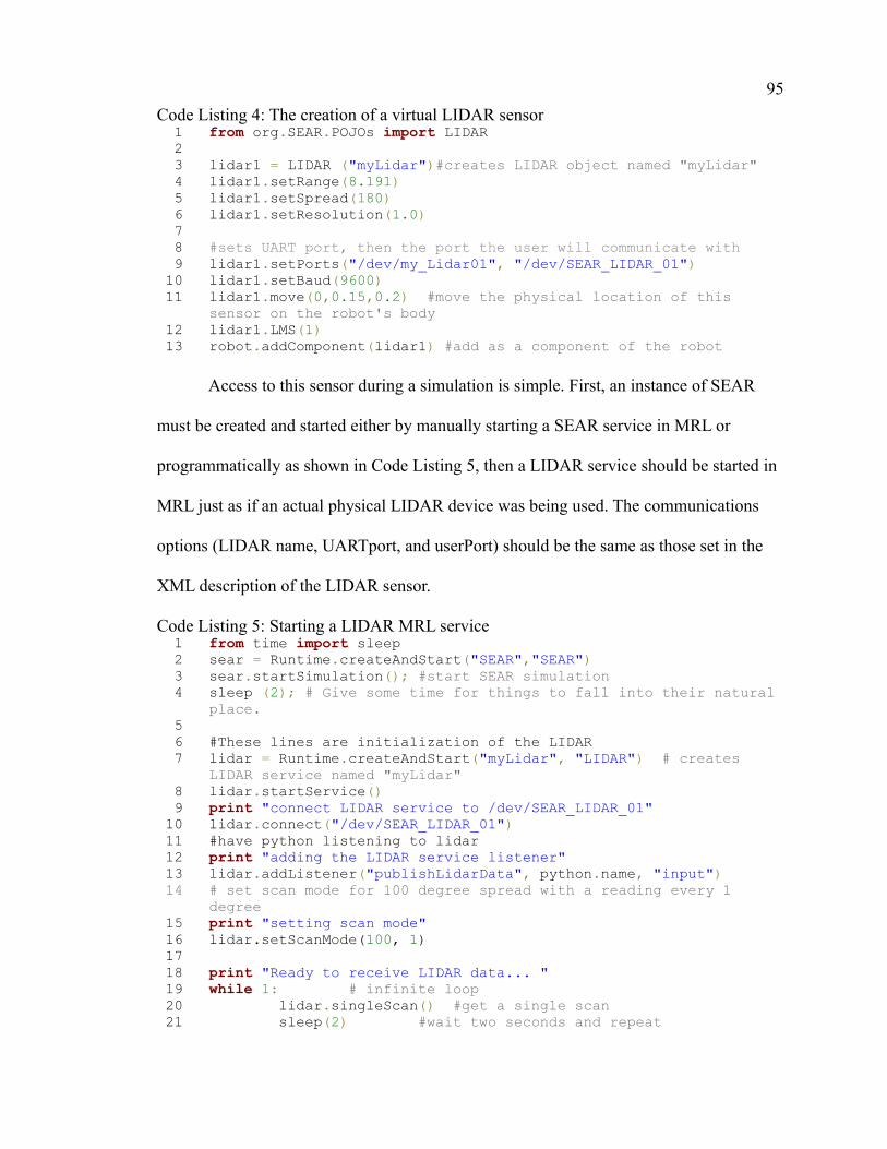
95
Code Listing 4: The creation of a virtual LIDAR sensor1 from org.SEAR.POJOs import LIDAR 23 lidar1 = LIDAR ("myLidar")#creates LIDAR object named "myLidar" 4 lidar1.setRange(8.191) 5 lidar1.setSpread(180) 6 lidar1.setResolution(1.0) 78 #sets UART port, then the port the user will communicate with 9 lidar1.setPorts("/dev/my_Lidar01", "/dev/SEAR_LIDAR_01") 10 lidar1.setBaud(9600) 11 lidar1.move(0,0.15,0.2) #move the physical location of this
sensor on the robot's body 12 lidar1.LMS(1) 13 robot.addComponent(lidar1) #add as a component of the robot
Access to this sensor during a simulation is simple. First, an instance of SEAR
must be created and started either by manually starting a SEAR service in MRL or
programmatically as shown in Code Listing 5, then a LIDAR service should be started in
MRL just as if an actual physical LIDAR device was being used. The communications
options (LIDAR name, UARTport, and userPort) should be the same as those set in the
XML description of the LIDAR sensor.
Code Listing 5: Starting a LIDAR MRL service1 from time import sleep 2 sear = Runtime.createAndStart("SEAR","SEAR") 3 sear.startSimulation(); #start SEAR simulation 4 sleep (2); # Give some time for things to fall into their natural
place. 5 6 #These lines are initialization of the LIDAR 7 lidar = Runtime.createAndStart("myLidar", "LIDAR") # creates
LIDAR service named "myLidar" 8 lidar.startService() 9 print "connect LIDAR service to /dev/SEAR_LIDAR_01" 10 lidar.connect("/dev/SEAR_LIDAR_01") 11 #have python listening to lidar 12 print "adding the LIDAR service listener" 13 lidar.addListener("publishLidarData", python.name, "input") 14 # set scan mode for 100 degree spread with a reading every 1
degree 15 print "setting scan mode" 16 lidar.setScanMode(100, 1) 1718 print "Ready to receive LIDAR data... " 19 while 1: # infinite loop 20 lidar.singleScan() #get a single scan 21 sleep(2) #wait two seconds and repeat

96
While the simulation is running, the LIDAR data can be viewed in the LIDAR
service tab named "myLidar" in MRL. This will update once each time the LIDAR
scans. To access the data of the LIDAR within the userCode script, a listener must be
added to the LIDAR service's publishLdarData method. This will call a userCode
method each time the LIDAR service receives a valid message. In Code Listing 6, the
listener calls the userCode method "input" each time the LIDAR service publishes data.
There are several examples (commented out) of how to use the raw LIDAR data. The
example that is not commented in this method will print the results out in the python
console window of MRL's python service as Cartesian coordinates of collisions using the
placement of the LIDAR in the simulated world as the reference (0,0).
Code Listing 6: Example code for accessing the raw LIDAR data1 from time import sleep 2 import Java.lang.String 3 import math 4 # This script only uses the LIDAR sensor on the simulated robot,
the user is expected to drive the robot using the i,j,k,l,and ; keys
56 def input(): 7 startingAngle = 0 8 code = msg_myLidar_publishLidarData.data[0] 9 length = len(code) 10 print "received " + str(length) +"readings:" 11 if length==101 or length==201 or length==401: 12 startingAngle = 40 13 else: 14 startingAngle = 0 15 16 for i in range(0, length): 17 # print hex(code[i]) #print result in hexadecimal 18 # print (code[i]) #print results (without units) 19 # print (code[i]/float(100)) #Print results in
centimeters (if LIDAR was in CM mode) 2021 # print ((code[i]/100)/2.54) #Print results in inches
(if LIDAR was in CM mode) 2223 # print str(i)+"\t"+str((code[i])) #print polar Coordinates
(without units) 24 #convert polar to Cartesian 25 x = (code[i])*math.cos(((i*100/length)+startingAngle)*
(3.14159 / 180))

97
Code Listing 6 Continued:26 y =(code[i])*math.sin(((i*100/length)+startingAngle)*
(3.14159 / 180)) 27 print str(x) +"\t"+str(y) 2829 # create and start the SEAR simulator instance 30 sear = Runtime.createAndStart("SEAR","SEAR") 31 sear.startSimulation(); #start SEAR simulation 32 sleep (2); # Give some time for things to fall into their natural
place. 33 34 print "Attempting to create the LIDAR service..."3536 #These lines are initialization of the LIDAR 37 lidar = Runtime.createAndStart("myLidar", "LIDAR") 38 lidar.startService() 39 print "connect LIDAR service to /dev/SEAR_LIDAR_01" 40 lidar.connect("/dev/SEAR_LIDAR_01") 4142 #have python listening to lidar 43 print "adding the LIDAR service listener" 44 lidar.addListener("publishLidarData", python.name, "input") 4546 # sets scan mode for 100 degree spread with a reading every 1
degree 47 print "setting scan mode" 48 lidar.setScanMode(100, 1) 4950 print "Ready to receive LIDAR data... " 51 while 1: # infinite loop 52 lidar.singleScan() #get a single scan 53 sleep(2) #wait two seconds and repeat
Note that in Code Listing 6, line 6 is the function that the userCode uses to access
the raw LIDAR service data. This line has to be constructed carefully to ensure it will
acquire the correct data. In this line, the variable getting loaded is called “code”. The
raw LIDAR data is stored in a variable which follows the format msg_<LIDAR service
name>_pubishLidatData[0]. The “<LIDAR service Name>” should be replaced with the
name of the LIDAR service created in this code. This can be seen in line 8: code =
msg_myLidar_publishLidarData.data[0], where “myLidar” is the name given to the
LIDAR sensor in line 37: lidar = Runtime.createAndStart("myLidar", "LIDAR"). It is
important to note that this variable will return as an array. Each element of this array will
contain the result of a LIDAR reading. The length of the array is determined by the

98
settings of a particular LIDAR scan.
A.5 Creating and Communicating with a Virtual GPS in SEAR
The user must first create the XML file for a GPS sensor in the robots folder of
the SEARProject. This is done easily by using a python script or Java class written
within MRL. The creation of the XML file will be done automatically in Code Listing 7.
Notice that the user must provide a starting GPS coordinate. This represents the starting
point of the robot and the center of the world.
Code Listing 7: Creation of a GPS sensor XML file for SEAR. This snippet should be added to Code Listing 2.
1 from org.SEAR.POJOs import GPS 2 # create a new GPS object (myGPS) with the name “gpsUnit1”3 myGPS = GPS("gpsUnit1", 33.61, 182.5, -80.865) 4 myGPS.setPorts("/dev/my_GPS_01","/dev/SEAR_GPS_01")5 robot.addComponent(myGPS)
There are two methods for users to access this sensor during a simulation. Firstly,
the user can see the results from GPGGA NMEA strings by initializing a GPS service in
MRL. This can be performed either manually (using the MRL GUI) or programmatically
using MRL's python or Java service. Figure 5.1.2 shows a screenshot of the GPS service
GUI printing data. To access the GPS data inside the userCode, the user can start a GPS
service in python or Java, then add a listener to that service. Code Listing 8 shows an
example that simply prints the resulting GPS values to the terminal. Note that the name of
the GPS agrees with the XML file. This is especially important in the lines that get the
GPS data.
Code Listing 8: Example code to access raw GPS data.1 from time import sleep 23 # This script only uses the GPS sensor on the simulated robot,
the user is expected to drive the robot using the i,j,k,l, and ; keys
45 sear = Runtime.createAndStart("SEAR","SEAR") 6 sear.startSimulation(); #start SEAR simulation

99
Code Listing 8 continued7 initialized = 0 89 gps1 = Runtime.createAndStart("gpsUnit1", "GPS") 10 gps1.startService() 11 gps1.connect("/dev/SEAR_GPS_01") 12 sleep(1) 13 def input(): 14 startingAngle = 0 15 Latitude = msg_gpsUnit1_publishGGAData.data[0][2] 16 Longitude = msg_gpsUnit1_publishGGAData.data[0][4] 17 altitude = msg_gpsUnit1_publishGGAData.data[0][9] 18 print "Lat: " + Latitude 19 print "Long: " + Longitude 20 print "Alt: " + altitude + "\n" 21 22 #have python listening to GPS 23 gps1.addListener("publishGGAData", python.name, "input") 2425 print "Ready to receive Data from GPS..."
A.6 Simple Sensors
Simple sensors are those which do not contain their own serial connection which
users can communicate with. This includes accelerometers, gyroscopes, compass
sensors, and the distance sensors. These sensors can be accessed in two ways; a very
simple method call to directly the simulator, or a by simulating a custom microelectronic
that handles the sensors and serial communications. This section describes the former
case.
Simple sensors can be accessed directly from userCode using method calls to the
simulator within the SEARservice. This interface is straightforward and can easily be
understood by users with little skill or knowledge of programming. The concept with this
implementation was to make it easy for users with little skill to access the sensors. The
aspiration is that SEAR would be used to help teach programming concepts such as
conditionals and loops. By having a simple method for accessing sensor data, the focus
of lessons could be on the overall programming concept rather than the specifics of
SEAR or MRL.

100
A.7 Custom Controller for Simple Sensors
For user who wish to more accurately emulate actual hardware, interfacing with
simple sensors (accelerometers, gyroscopes, compasses and distance sensors) happens by
proxy. In reality, the user would connect these sensors to a microcontroller which can
handle serial communications with userCode in MRL, and performs the actions required
to request and format data from these sensors. The processes of this microcontroller can
be simulated using a template python script provided with SEAR.
The communications protocol used by the template is based on the Roomba serial
protocol and is very simple to implement both in a simulation as well as with actual
hardware. The last “sensor command” in the Roomba protocol requests data from sensor
message number 42 [84]. SEAR’s custom controller accepts the same “sensor request
message” as the Roomba protocol, except it begins with number 43. Given that this is an
8-bit number, the user can add more than 200 additional commands.
The virtual controller handles the serial communications, parses the serial
commands, and selects the appropriate function to perform based on the command. Just
as would be required of actual hardware, functions must be supplied by the user. If the
command is received to “read the left ultrasonic sensor” then the user must insert code to
perform this action within the SEAR simulator. This simply consists of a call to SEAR's
ultrasonic sensor simulator class. Data is returned to this custom controller template
which then writes the data back on the serial port. When in use during a simulation,
abstraction allows this to be a black box to which a user issues commands and receives
data in return. This implementation is exactly the same as would be required to connect
to physical hardware. The pseudo-code in Table A.7 compares the code of a SEAR

101
virtual controller and a physical microcontroller.
Table A.7: Comparison of communications between userCode and physical hardware versus userCode and SEAR virtual hardware
Physical Microcontroller SEAR's Virtual Controller
User sends command via serial connection to the physical microcontroller to get a reading from the compass module. Usercode snippet:
1 Serial.writeByte(42) # sendsensor request
2 Serial.writeByte(30) # sensor “address”
User sends command via serial connection to the simulated controller object to get a reading from the compass module. Usercode snippet: 1 Serial.writeByte(42) # send
sensor request2 Serial.writeByte(30) #
sensor “address”
Command is sent via serial connection to the physical microcontroller
Command is sent via serial connection to the virtual controller object.
Microcontroller on the robot parses the command and calls the function to read the compass module's current value: (Microcontroller code snippet:)1 int heading =
getCompassValue(); #Assuminga function performs this forthe user.
Simulated controller object parses the command and calls the function to read the compass module's current value: (virtual controller code snippet:)1 int heading =
sear.getCompassResult("comp1")#The name of this sensor on the robot is in quotes to identify it from other sonar sensors that the robot might have.
Microcontroller on the robot sends data back to the user over the same serial port:2 Serial.writeInteger(heading)
Custom controller sends data back to the user over the same serial port: 2 Serial.writeInteger(heading)
The suggested method of using the custom controller is to send a request to the
controller’s serial port from the user’s code. The user should know the size of the
message the controller will return (this will be known since the user would have written
that code as well). The custom controller receives the message, parses it, performs the
selected action (such as taking the reading from the front-left ultrasonic sensor) then
returning the resulting data to the user’s code over its serial connection.
The custom controller code uses code written in a Python or Java file by the user
102
previous to running the simulation. The controller code simply utilizes MRL’s
virtualSerialPort objects to communicate to the main userCode (controlling the overall
simulation). The messages from this serial connection get parsed and a set of if
statements help select which action to perform. The user can choose to write custom
code for each if statement based on the needs and design of the robot.
To access SEAR’s simulated sensors the user will use methods from the SEAR
service. For the ultrasonic example above, the user would use code like
sear.getDistanceResult("leftFrontPing") which will return the distance in centimeters to
the nearest object that is within the range of that specific sensor. The name of the sensor,
leftFrontPing must match the name of the sensor in its XML file within the
SEARproject/robot folder. Once this value is acquired, it is sent back over the virtual
serial port to the user’s overall simulation code.
To simplify the process of creating a custom controller in SEAR, a template is
provided that listens for serial events on the virtual ports. There is also a list of empty “if”
statements with commented examples for each type of sensor. This template also has a
function to send the acquired data back to the main simulator. The suggested method of
using the custom controller is to send a request to the controller’s serial port from the
user’s code. The user should know the size of the message the controller will return (this
will be known since the user would have written that code as well). The custom controller
receives the message, parses it, performs the selected action (such as taking the reading
from the front-left ultrasonic sensor) then returning the resulting data to the user’s code
over its serial connection.
The custom controller code uses code written in a Python or Java file by the user

103
previous to running the simulation. The controller code simply utilizes MRL’s
virtualSerialPort objects to communicate to the main userCode (controlling the overall
simulation). The messages from this serial connection get parsed and a set of if
statements help select which action to perform. The user can choose to write custom
code for each if statement based on the needs and design of the robot.
The custom controller is implemented in a second python script (controller.py) in
addition to the user's code. Inside this script, there are functions for listening to a
specified virtual serial port, parsing the serial data, making the appropriate method calls
in SEAR simulator, and then a method for returning the data back over the virtual serial
port. The user must execute this file from a method call in the main userCode. Code
Listing 9 is an example for a custom controller that access multiple sensors. Users can
modify this template to match the specific sensor names used in their simulation and
desired sensor number (between 43 and 255, extended from the Roomba protocol sensor
data request commands).
This process becomes complicated when the controller attempts to send data back
to the userCode. The userCode must “listen” to its serial port “publishByte” command to
catch incoming messages from the controller. This “listener” method acts like an interrupt
that is triggered each time it receives a byte. The userCode must wait until all of the
bytes arrive before processing the data. A simple method for performing this action is
used in the pair of code listings for the simulated controller and userCode examples in
Code Listings 9 and 10 respectively. In this case, the user sets the expected size of the
message that will be returned, and clears the message buffers before sending the request
to the simulated controller. The userCode then runs a blocking method that compares the

104
current size of the received message with the expected size. When these values are equal,
the blocking method returns back to the main function. This is only one simple example
of how this may be accomplished. The userCode in listing 9 is only expecting data in big
endian two-byte format, though the user is free to change this to any format they wish.
Users are strongly encouraged to use the userCode and simulated controller code in
listings 9 and 10 respectively as templates for their custom implementations.
Debugging and testing of the simulated controller is simplest when the user
appends the current file name to the print statements used within the code, making it
easier to see which “thread” is printing at what time and in what order. Additionally, it
was found that for many data manipulation techniques used in this type of
implementation it was simpler to test the techniques in their own python scripts in MRL.
For example, for combining high byte and low byte of a two-byte array.
Code listings 9 and 10 contain the simulated virtual controller code and the
userCode that communicates with it respectively.
Code Listing 9: Example controller code named userCode.py1 from time import sleep 2 import sys 34 print "\n \n executing serial send" 5 python.execFile("controllerTest.py") #execute the simulated
controller's code 6 sleep(2) 78 currentLength = 0 9 messageLength = 2 10 msgBuffer = list() 11 msgResults = list() 121314 def sendControllerData(message): 15 #write a series of bytes to the serial port 16 serial.write(0x8E) #0x8E = 142 decimal which is the
"Sensor request" roomba opcode 17 serial.write(message) 18 from org.SEAR.POJOs import Cylinder 19 from org.SEAR.POJOs import Box

105
Code Listing 9 Continued:20 from org.SEAR.POJOs import Cone 21 from org.SEAR.POJOs import model2223 floor = Floor("floor", 50, 50) #create floor 2425 #create some obstacles 26 box = Box("Box1_name", 0.25, 0.25, 0.25, 0) 27 box.move(-1.5, 1.25, 0) 28 box.rotate(45, 0, 0) 2930 cyl = Cylinder("trash Can", 0.25, 0.75, 10) 31 cyl.move(-3, 0, -3.5) 32 cyl.rotate(0, 30, 30) 3334 coneA = Cone("Traffic Cone", 0.25, 2, 10) 35 coneA.move(-2, 0, 0) 36 coneA.rotate(0, 0, 45) 3738 tree = Model("Tree1_name","models/Tree/Tree.mesh.xml") 39 tree.move(0, 0, -3) 4041 print "Done creating Environment"4243 def receiveMessage(): 4445 global msgBuffer 46 global messageLeng--Add “Code Listing 1 Continued”
headings where required 47 global currentLength 48 global msgResults 49 50 data = msg_serial_publishByte.data[0] & 0xff 51 if (currentLength < messageLength): # if not the full
message, then store this in our buffer 52 msgBuffer.insert(currentLength, data) # fill the
message buffer full of bytes. 53 currentLength +=1 #increment index value 54 55 if (currentLength == messageLength): #otherwise, we are
at the last byte in the message, clear everything and parse into short ints 10
56 for i in range (0, messageLength, 2): # for i inrange(start, finish, step)
5758 if msgBuffer[i] >0 : 59 msgResults.insert(i/2, (msgBuffer
[i]<<8) + msgBuffer[i+1]) 60 elif msgBuffer[i] <0 : 61 msgResults.insert(i/2, 256+
(msgBuffer [i]<<8) + msgBuffer[i+1]) 6263 else: 64 msgResults.insert(i/2, 0x00ff &
msgBuffer[i+1]) 65

106
Code Listing 9 Continued:66 messageLength = 0 # reset this value to 0 so the
user knows when to check msgResults for values 67 currentLength = 0 6869 70 def waitForReply(): #this just constantly checks messageLength to
see if it is 0, indicating the data has been received completely. 71 global messageLength 72 while(messageLength != 0): 73 pass 747576 def clear(): 77 global currentLength 78 global msgBuffer 79 global msgResults 80 msgBuffer = [0,0,0,0,0,0,0] 81 msgResults = [0,0,0,0,0,0,0] 82 currentLength = 0 838485 #The below is the main function and actually calls the functions
above: 86 sear = Runtime.createAndStart("SEAR","SEAR") 8788 sear.startSimulation(); #start SEAR simulation 89 sleep(1) 90 roomba = Runtime.createAndStart("robot_Dynamics1","Roomba") 91 roomba.connect( "/dev/SEAR_Robot_01" ) 92 roomba.startup() 93 roomba.control() 94 sleep(1) 9596 #create a Serial service named serial 97 serial = Runtime.createAndStart("serial","Serial") 98 #connect to a serial port COM4 57600 bitrate 8 data bits 1 stop
bit 0 parity 99 serial.connect("/dev/user_CONTROLLER_01", 9600, 8, 1, 0) 100 101 serial.addListener("publishByte", python.name, "receiveMessage") 102 print "listening to: "+serial.name 103104105106 sleep(1) 107 print "Main: Requesting Sonar 1" 108 messageLength = 2 # set the number of bytes I expect the
controller to return (1 16-bit U-ints) 109 sendControllerData(0x2B) # get SONAR 1 reading 110 waitForReply() 111 print "\nBack in Main, Sonar 1 value received = " +
str(msgResults[0]) 112113114 print "Main: Requesting Sonar 2"

107
Code Listing 9 Continued:115 clear() 116 messageLength = 2 # set the number of bytes I expect the
controller to return (1 16-bit U-ints) 117 sendControllerData(0x2C) # get SONAR 1 reading 118 waitForReply() 119 print "\nBack in Main, Sonar 2 value received = " +
str(msgResults[0]) 120121122 print "Main Requesting Accel" 123 clear() 124 messageLength = 6 # set the number of bytes I expect the
controller to return (3 16-bit U-ints) 125 sendControllerData(0x2D) # get Accel readings (x, y, z) 126 waitForReply() 127 print "Back in Main, AccelX = " + str(msgResults[0]) +" AccelY = "
+ str(msgResults[1]) +" AccelZ = " + str(msgResults[2]) 128129130 print "Main Requesting Gyro" 131 clear() 132 messageLength = 6 # set the number of bytes I expect the
controller to return (3 16-bit U-ints) 133 sendControllerData(0x2E) # get Accel readings (x, y, z) 134 waitForReply() 135 print "Back in Main, GyroX = " + str(msgResults[0]) +" GyroY = " +
str(msgResults[1]) +" GyroZ = " + str(msgResults[2]) 136137138 print "Main Requesting Compass" 139 messageLength = 2 # set the number of bytes I expect the
controller to return (3 16-bit U-ints) 140 sendControllerData(0x2F) # get Compass reading 141 waitForReply() 142 # The compass sensor modeled here is the simple HMC6352 in
"heading" mode which will return a single value from 0-360.0 degrees in tenths of a degree (in steps of 0.5 degrees).
143 #Now we must divide by 10 because the HMC6352 outputs are from 0-3599 [https://www.sparkfun.com/datasheets/Components/HMC6352.pdf ]
144 print "Back in Main, Compass heading (out of 360 degrees) = " + str(float(msgResults[0])/10)
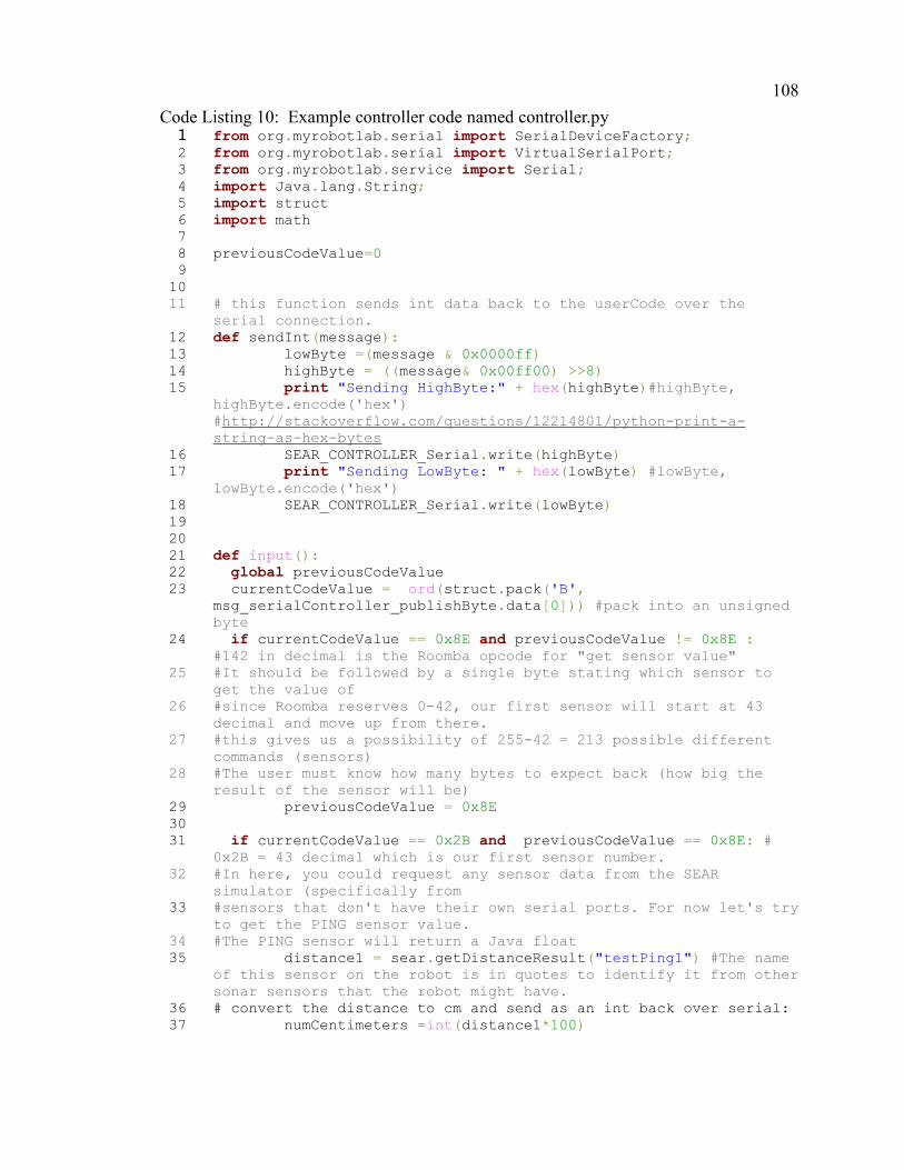
108
Code Listing 10: Example controller code named controller.py1 from org.myrobotlab.serial import SerialDeviceFactory; 2 from org.myrobotlab.serial import VirtualSerialPort; 3 from org.myrobotlab.service import Serial; 4 import Java.lang.String; 5 import struct 6 import math 78 previousCodeValue=0 91011 # this function sends int data back to the userCode over the
serial connection. 12 def sendInt(message): 13 lowByte =(message & 0x0000ff) 14 highByte = ((message& 0x00ff00) >>8)15 print "Sending HighByte:" + hex(highByte)#highByte,
highByte.encode('hex') #http://stackoverflow.com/questions/12214801/python-print-a-string-as-hex-bytes
16 SEAR_CONTROLLER_Serial.write(highByte) 17 print "Sending LowByte: " + hex(lowByte) #lowByte,
lowByte.encode('hex') 18 SEAR_CONTROLLER_Serial.write(lowByte) 1920 21 def input(): 22 global previousCodeValue 23 currentCodeValue = ord(struct.pack('B',
msg_serialController_publishByte.data[0])) #pack into an unsigned byte
24 if currentCodeValue == 0x8E and previousCodeValue != 0x8E : #142 in decimal is the Roomba opcode for "get sensor value"
25 #It should be followed by a single byte stating which sensor to get the value of
26 #since Roomba reserves 0-42, our first sensor will start at 43 decimal and move up from there.
27 #this gives us a possibility of 255-42 = 213 possible different commands (sensors)
28 #The user must know how many bytes to expect back (how big the result of the sensor will be)
29 previousCodeValue = 0x8E 3031 if currentCodeValue == 0x2B and previousCodeValue == 0x8E: #
0x2B = 43 decimal which is our first sensor number. 32 #In here, you could request any sensor data from the SEAR
simulator (specifically from 33 #sensors that don't have their own serial ports. For now let's try
to get the PING sensor value. 34 #The PING sensor will return a Java float 35 distance1 = sear.getDistanceResult("testPing1") #The name
of this sensor on the robot is in quotes to identify it from othersonar sensors that the robot might have.
36 # convert the distance to cm and send as an int back over serial: 37 numCentimeters =int(distance1*100)

109
Code Listing 10 Continued: 38 sendInt(int(distance1*100)) 39 40 if currentCodeValue == 0x2C and previousCodeValue == 0x8E:# 0x2C
= 44 decimal which is our second sensor number. 41 distance2 = sear.getDistanceResult("MyNewestSONAR") #The name of
this sensor on the robot is in quotes to identify it from other sonar sensors that the robot might have.
42 # convert the distance to cm and send as an int back over serial. 43 numCentimeters =int(distance2*100) 44 sendInt(int(distance2*100)) 454647 if currentCodeValue == 0x2D and previousCodeValue == 0x8E: #
0x2D = 45 decimal which is our third sensor number. 48 accelerations = sear.getAccelResult("accel") #This results
in a comma separated String containing X, Y and z respectively. We can simply parse the string to send the results.
4950 # convert each accel axis reading to a single int and send over
serial. 51 # SEAR's accelerometers output floats in meters/second^2. In the
ADXL330 for instance, each axis responds based on a measurements of "g-forces". We can assume that on the actual hardware, the microcontroller would handle converting the analog input from the accelerometers to meters/second^2 before it sends the values back as 3 ints: x, y, then z.
52 #In the ADXL330 though, 0Gs is at the midpoint of the analog output (if Vcc=3v, midpoint = 1.5volts) This will correspond to 10-bit resolution (in an Arduino for example) of about 512. So when an axis = 0G, the numeric value expected should be in the center of that range.
53 # the ADXL330 also has a 300mV/G resolution, so all of this information should be taken into account when formatting the data
54 tokens = accelerations.split(',') # Split my CSV string into individual number-strings
55 #from meters/sec^2 to #Gs 56 #number of Gs to mV/G, Make sure not to go higher than the range
of the ADXL330 +-3.6Gs 57 #from Gs to volts (range must be shifted so 1.5volts = 0Gs) 58 #from volts (what the ADXL330 outputs) to ADC steps 59 #(an arduino with 3.3v AREF using 10-bit ADC) = 310.30303 ADC
steps/volt 60 #send this ADC value back to MRL (userCode), so it can handle
converting it to useful values for a robot or filter it, etc. 61 62 integerAccelX = int((float(tokens[0]) /-9.8 * 0.3 + 1.5)*
310.30303) 63 if integerAccelX >1023: 64 integerAccelX = 1023 65 #integerAccelX = int(float(tokens[0])) 6667 integerAccelY = int((float(tokens[1]) /-9.8 * 0.3 + 1.5)*
310.30303) 68 69

110
Code Listing 10 Continued:70 if integerAccelY >1023: 71 integerAccelY= 1023 72 integerAccelZ = int((float(tokens[2]) /-9.8 * 0.3 + 1.5)*
310.30303) 73 if integerAccelZ >1023: 74 integerAccelZ = 1023 75 print "accel ints = "+ str(integerAccelX)+", "+
str(integerAccelY)+", "+ str(integerAccelZ) 76 print "hex accel ints = "+ hex(integerAccelX)+", "+
hex(integerAccelY)+", "+ hex(integerAccelZ) 77 sendInt(integerAccelX) # Sending X acceleration value 78 sendInt(integerAccelY) # Sending Y acceleration value 79 sendInt(integerAccelZ) # Sending Z acceleration value 808182 if currentCodeValue == 0x2E and previousCodeValue == 0x8E: #
0x2E = 46 decimal which is our fourth sensor number. 83 gyroReadings = sear.getGyroResult("gyro1") #SEAR's Gyro
returns a CSV string of angular velocities (in radians) Let's convert these into the nearest integer value of rad/sec
84 tokens = gyroReadings.split(',') # Split the CSV string into individual number-strings
858687 # SEAR's Gyroscope returns values in radians / second. 88 # In this example, we will mimic the IDG500 (which normally has 2
axis, but we will scale all 3 the same. 89 #the IDG500 returns values on an analog output. Its datasheet
values are for a VCC of 3.0 volts (not 3.3) 90 # The value is scaled 2mv / (degree/second) and the output at 0 =
1.35v. There are 57.2957795 degrees per radian 91 # If we are using an arduino with a AREF of 3.3v, that = 310.30303
ADC steps / volt 92 93 integerGyroX = int(((float(tokens[0])*57.2957795 * 0.002)+
1.35)*310.30303) 94 integerGyroY = int(((float(tokens[1])*57.2957795 * 0.002)+
1.35)*310.30303) 95 integerGyroZ = int(((float(tokens[2])*57.2957795 * 0.002)+
1.35)*310.30303) 96 sendInt(integerGyroX) # Sending X Gyro value 97 sendInt(integerGyroY) # Sending Y Gyro value 98 sendInt(integerGyroZ) # Sending Z Gyro value 99100101 if currentCodeValue == 0x2F and previousCodeValue == 0x8E: #
0x2F = 47 decimal which is our fifth sensor number. 102 rawHeading = sear.getCompassResult("comp1") #The name of
this sensor on the robot is in quotes to identify it from other sonar sensors that the robot might have.
103 #Note that SEAR returns +-180 degrees, so we must make this 0-360:104 if rawHeading < 0: 105 rawHeading = rawHeading + 360 106107

111
Code Listing 10 Continued:108 # The compass sensor modeled here is the simple HMC6352 in
"heading" mode which will return a single value from 0-360.0 degrees in tenths of a degree (in steps of 0.5 degrees). The simulated SEARcompass returns a float from 0-360.
109 #We must convert the SERAcompass value to mimic the outputof the HMC6352. So we will first round to the nearest 0.5 degrees. :
110 heading = 0.5 * math.ceil(2.0 * rawHeading) #rounds to thenearest 0.5 http://stackoverflow.com/questions/9758513/how-can-i-round-up-numbers-to-the-next-half-integer
111 #Now we must multiply by 10 because the HMC6352 outputs are from 0-3599 [https://www.sparkfun.com/datasheets/Components/HMC6352.pdf ]
112 intHeading = int(heading*10) # convert this to an integer after it is multiplied, giving us a range of 0-3599
113 sendInt(intHeading) # Now send it back to the userCodeon the virtual serial port
114115116 # main function code goes below here. 117 UARTport = "/dev/my_Controller01" 118 userPort = "/dev/user_CONTROLLER_01" 119120121 #Create two virtual ports for UART and user and null them
together: 122 # create 2 virtual ports 123 vp0 = VirtualSerialPort(UARTport); 124 vp1 = VirtualSerialPort(userPort); 125126 # make null modem cable ;) 127 VirtualSerialPort.makeNullModem(vp0, vp1); 128129 # add virtual ports to the serial device factory 130 SerialDeviceFactory.add(vp0); 131 SerialDeviceFactory.add(vp1); 132133 # create the UART serial service 134 SEAR_CONTROLLER_Serial =
Runtime.createAndStart("serialController","Serial") 135 SEAR_CONTROLLER_Serial.connect(UARTport); 136137 #have controller listening to userCode 138 SEAR_CONTROLLER_Serial.addListener("publishByte", python.name,
"input") 139 print "user should connect to port named: "+userPort