Environment Centered Analysis and Design ofCoordination Mechanisms

Keith S. Decker

UMass CMPSCI Technical Report 95-69May 1995

Department of Computer ScienceUniversity of MassachusettsAmherst MA 01003-4610

EMAIL: decker@cs.umass.edu

This work was supported by DARPA contract N00014-92-J-1698, Office of Naval Research contract N00014-92-J-1450, and NSF contract CDA 8922572. The content of the information does not necessarily reflect theposition or the policy of the Government and no official endorsement should be inferred.

ENVIRONMENT CENTERED ANALYSIS AND DESIGN OF COORDINATION MECHANISMS

A Dissertation Presented

by

KEITH S. DECKER

Submitted to the Graduate School of theUniversity of Massachusetts Amherst in partialfulfillment of the requirements for the degree of

DOCTOR OF PHILOSOPHY

May 1995

Department of Computer Science

c Copyright by Keith S. Decker 1995

All Rights Reserved

To my parents, Lafeyette J. and Phyllis J. Decker.

iv

ACKNOWLEDGMENTS

When I left General Electric to return to graduate school for my Ph.D., I applied to onlyone place, UMass, to work with one person, Victor Lesser, on Distributed AI. My deepestthanks to Victor for his guidance, mentoring, and support over the years; Vic pushed me to domore than I thought I could.

I’d like to thank the other members of my committee as well. Paul Cohen suppliedinvaluable guidance on the statistical analyses in this thesis, as well as reminding me when Ifailed to remember Tufte’s graphical principles. Most importantly, Paul acted as my secondmentor here at UMass and his interest in methodology for AI was a catalyst that made thestructure of my thesis crystallize for me several years before I completed it. Jack Stankovic wasa tough reader who hounded me into avoiding the jargon of DAI and keeping this work opento other computer scientists; he reminded me of how my work interacts with that of traditionaldistributed computing. Doug Anderton also helped point out my methodological failings andquite a bit of organizational theory literature; he encouraged me to try to open the thesis toreaders outside of computer science entirely.

The DAI research community is a friendly and helpful one, and I’d like to thank everyonethere for their intellectual stimulus, especially Susan Conrey, Ed Durfee, Eithan Ephrati, SteveFickas, Piotr Gmytrasiewicz, Mike Huhns, Frank v. Martial, Jeff Rosenschein, and KatiaSycara. A very special thanks goes to Les Gasser, who has continuously reminded me of thesocial aspects of DAI research and who has always supported that direction in my work.

A very special technical thanks to Alan ‘Bart’ Garvey, who wrote the Design-To-Time localscheduler (that’s part of his thesis) used in this thesis—the collaboration has been amazinglyfruitful. I’d also like to thank Bart for his gourmet cooking, shipping microbrewery beer andsalmon from Seattle, help in brewing (coffee and beer), and his taste in wine.

Many other people have become my friends here and have offered support and encour-agement over the years. A special thanks to my extended family, the Westbrooks (David, Teri,Brian, and Josh), who supplied food, washing machine and dryer, gardening advice & supplies,sewing machine, indoor and outdoor recreational activities, and parties. Thanks to the othercurrent and former members of the DIS lab who have been happy to exchange ideas and to putup with proofreading my research papers: Dave Hildum, Marty Humphrey, Dan Neiman, BobWhitehair, Nagi, Quin (the Alpha Man), Dorothy Mammon, and Sue Lander. I should notethat Dave provided the LATEX style files for this thesis, Marty provided the parallel scheduler Italk about in Chapter 6, and Dann has surely been saddled with reading more of my papersthan anyone.

Starting someplace new is always hard, and I made many friends here my first year thathave remained friends since. Thanks to Claire Cardie, Lauren Halverson, Alan Kaplan, SueMathisen, Doug Niehaus, and Ellen Riloff. Many other friends followed, and I’ve partaken oftheir hospitality and/or software experience many times: Scott Anderson, Carla Brodley, CarolBroverman (thanks for the house), Jody Daniels, Tony Hosking, Alice P. Julier, Ruth Kaplan,Joe McCarthy (homebrewer), Zack Rubinstein (Emacs hacker), and David Skalak. Thanks tothe Amalgams for giving me something to do over the summers. Thanks to the RCF staff,especially Steve, Terrie, and Glenn.

v

In a very real way I returned to graduate school to get my Ph.D. due to the supportand encouragement of Piero Bonissone, to whom I remain indebted. Special thanks to JimAragones for dragging me out of Amherst and back to Schenectady for some fun once in awhile.

I should also thank the people at CMU who got me interested in AI, and taught me AI froma cognitive perspective (from which a social perspective on DAI seems a natural one): HerbSimon, Jill Larkin, Elaine Kant, and John Anderson. Thanks to Doc Moore for convincingme to be a math major instead of a physics major. Thanks to Mike and Joan Mintz for alsodragging me out of Amherst once in a while.

Finally, a big thanks to my parents for their financial and emotional support through this(very) long process!

vi

ABSTRACT

Environment Centered Analysis and Design of Coordination Mechanisms

May 1995

KEITH S. DECKER

B.S., Carnegie Mellon UniversityM.S., Rensselaer Polytechnic Institute

Ph.D., University of Massachusetts Amherst

Directed by: Professor Victor R. LesserCommittee: Professor Paul R. Cohen

Professor John A. StankovicProfessor Douglas L. Anderton

Coordination, as the act of managing interdependencies between activities, is one of thecentral research issues in Distributed Artificial Intelligence. Many researchers have shown thatthere is no single best organization or coordination mechanism for all environments. Problemsin coordinating the activities of distributed intelligent agents appear in many domains: thecontrol of distributed sensor networks; multi-agent scheduling of people and/or machines;distributed diagnosis of errors in local-area or telephone networks; concurrent engineering;‘software agents’ for information gathering.

The design of coordination mechanisms for groups of computational agents depends inmany ways on the agent’s task environment. Two such dependencies are on the structureof the tasks and on the uncertainty in the task structures. The task structure includes thescope of the problems facing the agents, the complexity of the choices facing the agents, andthe the particular kinds and patterns of interrelationships that occur between tasks. A fewexamples of environmental uncertainty include uncertainty in the a priori structure of anyparticular problem-solving episode, in the actions of other agents, and in the outcomes of anagent’s own actions. These dependencies hold regardless of whether the system comprises justpeople, computational agents, or a mixture of the two. Designing coordination mechanismsalso depends on properties of the agents themselves.

Our thesis is that the design of coordination mechanisms cannot rely on the principledconstruction of agents alone, but must also rely on the structure and other characteristics of theagents’ task environment. For example, the presence of both uncertainty and high variance ina task structure can lead to better performance in coordination algorithms that adapt to eachproblem-solving episode. Furthermore, the structure and characteristics of an environmentcan and should be used as the central guide to the design of coordination mechanisms, andthus must be a part of our eventual goal, a comprehensive theory of coordination, partiallydeveloped here.

vii

Our approach is to first develop a framework, TÆMS, to directly represent the salientfeatures of a computational task environment. The unique features of TÆMS include that itquantitatively represents complex task interrelationships, and that it divides a task environmentmodel into generative, objective, and subjective levels. We then extend a standard methodologyto use the framework and apply it to the first published analysis, explanation, and predictionof agent performance in a distributed sensor network problem. We predict the effect of addingmore agents, changing the relative cost of communication and computation, and changing howthe agents are organized. Finally, we show how coordination mechanisms can be designed torespond to particular features of the task environment structure by developing the GeneralizedPartial Global Planning (GPGP) family of algorithms. GPGP is a cooperative (team-oriented)coordination component that is unique because it is built of modular mechanisms that workin conjunction with, but do not replace, a fully functional agent with a local scheduler. GPGPdiffers from other previous approaches in that it is not tied to a single domain, it allowsagent heterogeneity, it exchanges less global information, it communicates at multiple levelsof abstraction, and it allows the use of a separate local scheduling component. We provethat GPGP can be adapted to different domains, and learn what its performance is throughsimulation in conjunction with a heuristic real-time local scheduler and randomly generatedabstract task environments.

viii

TABLE OF CONTENTS

ACKNOWLEDGMENTS : : : : : : : : : : : : : : : : : : : : : : : : : : : : : : : : : : : : : : : : v

ABSTRACT : : : : : : : : : : : : : : : : : : : : : : : : : : : : : : : : : : : : : : : : : : : : : : : : : vii

LIST OF TABLES : : : : : : : : : : : : : : : : : : : : : : : : : : : : : : : : : : : : : : : : : : : : : xiv

LIST OF FIGURES : : : : : : : : : : : : : : : : : : : : : : : : : : : : : : : : : : : : : : : : : : : : xv

CHAPTERS

1. INTRODUCTION: WHY STUDY COORDINATION? : : : : : : : : : : : : : : : : : : : : : : : 1

1.1 Representing Task Environments : : : : : : : : : : : : : : : : : : : : : 21.2 Analyzing a Distributed Sensor Network Environment : : : : : : : : : : : 41.3 Designing a Family of Coordination Mechanisms : : : : : : : : : : : : : 51.4 Placing This Work in a Context : : : : : : : : : : : : : : : : : : : : : : 7

1.4.1 Scope : : : : : : : : : : : : : : : : : : : : : : : : : : : : : : : 91.4.2 Applications : : : : : : : : : : : : : : : : : : : : : : : : : : : : 10

1.5 Chapter Summary : : : : : : : : : : : : : : : : : : : : : : : : : : : : : 12

2. RELATED RESEARCH : : : : : : : : : : : : : : : : : : : : : : : : : : : : : : : : : : : : : : : : : : 13

2.1 Task Environments : : : : : : : : : : : : : : : : : : : : : : : : : : : : 13

2.1.1 Example Task Environments : : : : : : : : : : : : : : : : : : : 15

2.2 What is Coordination Behavior: The Social View : : : : : : : : : : : : : 15

2.2.1 What is Coordination Behavior: Rational Systems : : : : : : : : : 162.2.2 What is Coordination Behavior: Natural Systems and Institutions : 172.2.3 What is Coordination Behavior: Open Systems : : : : : : : : : : 182.2.4 What is Coordination Behavior: Economic Systems : : : : : : : : 19

2.3 How Does the Environment Affect Coordination Behavior: The Social View 20

2.3.1 How Does the Environment Affect Coordination Behavior: Con-tingency Theory : : : : : : : : : : : : : : : : : : : : : : : : : : 22

2.3.1.1 Definitions : : : : : : : : : : : : : : : : : : : : : : : 22

2.3.2 How Does the Environment Affect Coordination Behavior: Infor-mation Processing : : : : : : : : : : : : : : : : : : : : : : : : : 26

2.3.3 How Does the Environment Affect Coordination Behavior: Principal-Agent Theory and Transaction Costs Economics : : : : : : : : : : 27

2.3.3.1 Principal-agent Theory : : : : : : : : : : : : : : : : : 28

ix

2.3.3.2 Transaction Costs Economics : : : : : : : : : : : : : : 29

2.3.4 How Does the Environment Affect Coordination Behavior: SocialStructural Analysis : : : : : : : : : : : : : : : : : : : : : : : : 30

2.3.5 Summary: How Does the Environment Affect Coordination Behavior—The Social View : : : : : : : : : : : : : : : : : : : : : : : : : : 30

2.4 What is Coordination Behavior: DAI Perspective : : : : : : : : : : : : : 31

2.4.1 Malone’s Organizational Models : : : : : : : : : : : : : : : : : : 332.4.2 Partial Global Planning : : : : : : : : : : : : : : : : : : : : : : 332.4.3 Hierarchical Behavior Space : : : : : : : : : : : : : : : : : : : : 342.4.4 Distributed AI and the Concept of Agency : : : : : : : : : : : : 352.4.5 Distributed AI and Distributed Processing : : : : : : : : : : : : : 36

2.4.5.1 Decentralized Control Theory : : : : : : : : : : : : : 362.4.5.2 Team Theory : : : : : : : : : : : : : : : : : : : : : : 372.4.5.3 Distributed OS Job Scheduling : : : : : : : : : : : : : 382.4.5.4 Game Theory : : : : : : : : : : : : : : : : : : : : : 39

2.5 DAI Modeling : : : : : : : : : : : : : : : : : : : : : : : : : : : : : : 412.6 Summary : : : : : : : : : : : : : : : : : : : : : : : : : : : : : : : : : 41

3. A FRAMEWORK FOR MODELING TASK ENVIRONMENTS : : : : : : : : : : : : : : : : : : : 43

3.1 General Framework : : : : : : : : : : : : : : : : : : : : : : : : : : : : 443.2 TÆMS model summary : : : : : : : : : : : : : : : : : : : : : : : : : : 45

3.2.1 Objective task structure summary : : : : : : : : : : : : : : : : : 453.2.2 The subjective mapping and agent actions : : : : : : : : : : : : : 463.2.3 Coordination Problems : : : : : : : : : : : : : : : : : : : : : : 47

3.3 Distributed Sensor Network Example : : : : : : : : : : : : : : : : : : : 483.4 TÆMS Objective Level Models : : : : : : : : : : : : : : : : : : : : : : : 50

3.4.1 Local Effects: The Subtask Relationship : : : : : : : : : : : : : : 513.4.2 Local Effects: Method Quality : : : : : : : : : : : : : : : : : : 523.4.3 Non-local Effects : : : : : : : : : : : : : : : : : : : : : : : : : 53

3.4.3.1 Non-local Effect Examples : : : : : : : : : : : : : : : 543.4.3.2 An Example of Facilitates and Shares-results : : : : : : : 58

3.4.4 Expanding the DSN Model : : : : : : : : : : : : : : : : : : : : 593.4.5 Resources : : : : : : : : : : : : : : : : : : : : : : : : : : : : : 62

3.5 TÆMS Subjective Level Models and Agent Actions : : : : : : : : : : : : : 65

3.5.1 The Subjective Mapping : : : : : : : : : : : : : : : : : : : : : 663.5.2 Deciding What to Do Next: Coordination, Scheduling, and Control 663.5.3 Computation : : : : : : : : : : : : : : : : : : : : : : : : : : : 67

3.5.3.1 Method Execution : : : : : : : : : : : : : : : : : : : 683.5.3.2 Communication : : : : : : : : : : : : : : : : : : : : 683.5.3.3 Information Gathering : : : : : : : : : : : : : : : : : 69

x

3.5.4 Subjective Modeling Example : : : : : : : : : : : : : : : : : : : 693.5.5 Sugawara’s Network Diagnosis System : : : : : : : : : : : : : : : 70

3.6 TÆMS Generative Level Models and Framework Examples : : : : : : : : : 71

3.6.1 The Generative Level : : : : : : : : : : : : : : : : : : : : : : : 713.6.2 The TÆMS Simulator Generator : : : : : : : : : : : : : : : : : : 723.6.3 Examples : : : : : : : : : : : : : : : : : : : : : : : : : : : : : 73

3.6.3.1 Hospital Patient Scheduling : : : : : : : : : : : : : : 743.6.3.2 Airport Resource Management : : : : : : : : : : : : : 763.6.3.3 Internet Information Gathering : : : : : : : : : : : : : 783.6.3.4 Pilot’s Associate : : : : : : : : : : : : : : : : : : : : : 81

3.7 Summary : : : : : : : : : : : : : : : : : : : : : : : : : : : : : : : : : 82

4. DESIGN AND ANALYSIS OF COORDINATION ALGORITHMS: A TASK ENVIRONMENT

MODEL FOR A SIMPLE DSN ENVIRONMENT : : : : : : : : : : : : : : : : : : : : : : : : : : : : 85

4.1 Task Environment Simulation : : : : : : : : : : : : : : : : : : : : : : : 864.2 Expected Number of Sensor Subtasks : : : : : : : : : : : : : : : : : : : 87

4.2.1 Distribution of the Binomial Max Order Statistic : : : : : : : : : 89

4.3 Expected Number of Task Groups : : : : : : : : : : : : : : : : : : : : : 904.4 Expected Number of Agents : : : : : : : : : : : : : : : : : : : : : : : : 904.5 Work Involved in a Task Structure : : : : : : : : : : : : : : : : : : : : : 91

4.5.1 Execution Model : : : : : : : : : : : : : : : : : : : : : : : : : 924.5.2 Simple Objective DSN Model : : : : : : : : : : : : : : : : : : : 92

4.6 Model Summary : : : : : : : : : : : : : : : : : : : : : : : : : : : : : 934.7 Static vs. Dynamic Organizational Structures: Reorganizing to Balance

System Load : : : : : : : : : : : : : : : : : : : : : : : : : : : : : : : : 94

4.7.1 Analyzing Static Organizations : : : : : : : : : : : : : : : : : : 944.7.2 Control Costs : : : : : : : : : : : : : : : : : : : : : : : : : : : 974.7.3 Analyzing Dynamic Organizations : : : : : : : : : : : : : : : : 984.7.4 Dynamic Coordination Algorithm for Reorganization : : : : : : : 1004.7.5 Analyzing the Dynamic Restructuring Algorithm : : : : : : : : : 102

4.7.5.1 Increasing Task Durations : : : : : : : : : : : : : : : 102

4.8 Using Meta-Level Communication : : : : : : : : : : : : : : : : : : : : 1054.9 Summary : : : : : : : : : : : : : : : : : : : : : : : : : : : : : : : : : 113

5. GENERALIZED PARTIAL GLOBAL PLANNING : : : : : : : : : : : : : : : : : : : : : : : : : : 117

5.1 Partial Global Planning : : : : : : : : : : : : : : : : : : : : : : : : : : 119

5.1.1 Issues in Extending the PGP Mechanisms : : : : : : : : : : : : : 122

5.1.1.1 Heterogeneous Agents : : : : : : : : : : : : : : : : : 1225.1.1.2 Dynamic Agents : : : : : : : : : : : : : : : : : : : : 123

xi

5.1.1.3 Real-time Agents : : : : : : : : : : : : : : : : : : : : 123

5.2 Generalizing the Partial Global Planning Mechanisms : : : : : : : : : : : 124

5.2.1 Uncertainty : : : : : : : : : : : : : : : : : : : : : : : : : : : : 1255.2.2 Task Interrelationships : : : : : : : : : : : : : : : : : : : : : : 125

5.3 Generalized Partial Global Planning: Conceptual Overview : : : : : : : : 1265.4 The Agent Architecture : : : : : : : : : : : : : : : : : : : : : : : : : : 1285.5 The Local Scheduler : : : : : : : : : : : : : : : : : : : : : : : : : : : : 1295.6 The Coordination Mechanisms : : : : : : : : : : : : : : : : : : : : : : 130

5.6.1 The Substrate Mechanisms : : : : : : : : : : : : : : : : : : : : 1305.6.2 Mechanism 1: Updating Non-Local Viewpoints : : : : : : : : : : 1325.6.3 Mechanism 2: Communicating Results : : : : : : : : : : : : : : 1335.6.4 Mechanism 3: Handling Simple Redundancy : : : : : : : : : : : 1335.6.5 Mechanism 4: Handling Hard Coordination Relationships : : : : 1365.6.6 Mechanism 5: Handling Soft Coordination Relationships : : : : : 136

5.7 Interfacing the Coordination Mechanism with the Local Scheduler : : : : : 137

5.7.1 Scheduler Inputs : : : : : : : : : : : : : : : : : : : : : : : : : 1395.7.2 Scheduler Output : : : : : : : : : : : : : : : : : : : : : : : : : 1415.7.3 Interfacing the Coordination Mechanism with the Local Scheduler:

Discussion : : : : : : : : : : : : : : : : : : : : : : : : : : : : 144

5.8 Summary : : : : : : : : : : : : : : : : : : : : : : : : : : : : : : : : : 145

6. EXPERIMENTS IN GENERALIZED PARTIAL GLOBAL PLANNING : : : : : : : : : : : : : : : 147

6.1 Initial Experiments: The Effect of Facilitation Power and Likelihood : : : : 148

6.1.1 Calculating Delays : : : : : : : : : : : : : : : : : : : : : : : : 1506.1.2 A Simple Model of the Utility of Detecting Facilitates : : : : : : : 1516.1.3 When to Detect and Communicate Facilitates : : : : : : : : : : : 1526.1.4 Facilitating Real-time Performance : : : : : : : : : : : : : : : : 1536.1.5 Delay : : : : : : : : : : : : : : : : : : : : : : : : : : : : : : : 156

6.2 GPGP Simulation: Issues : : : : : : : : : : : : : : : : : : : : : : : : : 1586.3 General Performance Issues : : : : : : : : : : : : : : : : : : : : : : : : 1586.4 Taking Advantage of a Coordination Relationship: When to Add a New

Mechanism : : : : : : : : : : : : : : : : : : : : : : : : : : : : : : : : 1606.5 Different Family Members for Different Environments : : : : : : : : : : : 1616.6 Meta-level Communication: Return to Load Balancing through Dynamic

Reorganization : : : : : : : : : : : : : : : : : : : : : : : : : : : : : : 1636.7 Computational Organizational Design : : : : : : : : : : : : : : : : : : : 164

6.7.1 Burton and Obel Experiments : : : : : : : : : : : : : : : : : : : 165

6.8 Exploring the Family Performance Space : : : : : : : : : : : : : : : : : : 1676.9 Summary : : : : : : : : : : : : : : : : : : : : : : : : : : : : : : : : : 170

xii

7. CONCLUSIONS : : : : : : : : : : : : : : : : : : : : : : : : : : : : : : : : : : : : : : : : : : : : : 175

7.1 Summary: Representing Task Environments : : : : : : : : : : : : : : : : 1757.2 Summary: Analyzing a Distributed Sensor Network Environment : : : : : 1777.3 Summary: Designing a Family of Coordination Mechanisms : : : : : : : : 1777.4 Limitations of this work : : : : : : : : : : : : : : : : : : : : : : : : : : 1807.5 Future Work : : : : : : : : : : : : : : : : : : : : : : : : : : : : : : : 181

REFERENCES : : : : : : : : : : : : : : : : : : : : : : : : : : : : : : : : : : : : : : : : : : : : : : : 187

xiii

LIST OF TABLES

6.1 Average percent quality increase for various commitment delay values. : : : : : : 157

6.2 Environmental Parameters used to generate the random episodes : : : : : : : : 158

6.3 Overhead associated with individual mechanisms at each parameter setting : : : 159

6.4 Performance comparison: Centralized Parallel Scheduler vs. Balanced GPGPCoordination and Decentralized DTT Scheduler : : : : : : : : : : : : : : 161

6.5 Performance comparison: Simple GPGP Coordination vs. Balanced GPGPCoordination : : : : : : : : : : : : : : : : : : : : : : : : : : : : : : : : 161

6.6 Parameters used to generate the 40 random episodes : : : : : : : : : : : : : : 166

6.7 Complete KMEANS linear clustering output for all 72 agent types, first threeclusters. All performance parameters were standardized within blocks. : : : : 171

6.8 Complete KMEANS linear clustering output for all 72 agent types, continued.All performance parameters were standardized within blocks. : : : : : : : : 172

xiv

LIST OF FIGURES

2.1 Secret agents A and B are captured and must decide whether to “Cooperate” withone another, or to “Defect”. : : : : : : : : : : : : : : : : : : : : : : : : : 40

3.1 Examples of 18 � 18 DSN organizations : : : : : : : : : : : : : : : : : : : : 49

3.2 Objective task structure associated with a single vehicle track. : : : : : : : : : : 50

3.3 Objective task structure associated with visiting the post office to buy stampsand/or mail a package. Assume that every agent has a local method for eachof these tasks. : : : : : : : : : : : : : : : : : : : : : : : : : : : : : : : : 58

3.4 A simple model of two tasks with two methods each. : : : : : : : : : : : : : : 59

3.5 Quality at each Method, Task, and Task Group over time in the previous figure : 60

3.6 Objective task structure associated with two agents : : : : : : : : : : : : : : : 61

3.7 Non-local effects in the objective task structure : : : : : : : : : : : : : : : : : 62

3.8 Example of two methods sharing a limited resource of capacity 15. In this example,if both methods execute in temporally overlapping time periods, the durationsof each method will be lengthened by 50%. : : : : : : : : : : : : : : : : : 63

3.9 Example objective structure of two methods (M1 and M3) that consume a resource,and one method that replenishes it. : : : : : : : : : : : : : : : : : : : : : 64

3.10 The finite state machine that describes the meta-structure of single-processor agentcomputations. I; C;M are named subsets of the agents beliefs� that representinformation gathering, communication, and method execution actions, respectively. 67

3.11 Example of what is learned in the network diagnosis problem: the correctscheduling strategy for each objective situation, and the knowledge of whichsituation is currently occurring. : : : : : : : : : : : : : : : : : : : : : : : 70

3.12 High-level, objective task structure and subjective views for a typical hospitalpatient scheduling episode. The top task in each ancillary is really the sameobjective entity as the unit task it is linked to in the diagram. : : : : : : : : 74

3.13 Objective task structure for a small airport resource management episode. : : : : 77

3.14 High-level, objective task structure for a two independent queries that resolve atone point to a single machine. : : : : : : : : : : : : : : : : : : : : : : : 79

xv

3.15 Mid-level, objective task structure for a single query for a review of a Macintoshproduct showing intra-query relationships. : : : : : : : : : : : : : : : : : 80

3.16 Dynamic Situations in Pilot’s Associate. All tasks accrue quality with Min (AND). 82

4.1 Examples of DSN organizations on an 18 � 18 grid : : : : : : : : : : : : : : : 86

4.2 A comparison of the probability distributions of the outcome of ‘heads’ in the actof flipping a coin 10 times (the binomial b10;0:5(s)) compared to the outcomeof having 2, 5, or 10 agents flip 10 coins and taking the number of headsof the agent who flipped the most heads (the max order statistics g2;10;0:5(s)through g10;10;0:5(s)). : : : : : : : : : : : : : : : : : : : : : : : : : : : : 88

4.3 Actual versus predicted heaviest load SN for various values of A, r, o, and N : : 89

4.4 On the left, actual versus predicted maximum number of task groups (tracks) seenby any one agent for various r, A, and n. On the right, actual versus predictedaverage number of agents seeing a single task group (track) for various r, o,and A. : : : : : : : : : : : : : : : : : : : : : : : : : : : : : : : : : : : 91

4.5 Objective task structure associated with a single vehicle track. : : : : : : : : : : 93

4.6 Example of a 3x3 organization, r = 11, o = 5, with 5 tracks. The thick dark greyboxes outline the default static organization, where there is no overlap. : : : 95

4.7 Detail from the previous figure of the processing that takes place on the trackrunning from (1,17) to (16,1) : : : : : : : : : : : : : : : : : : : : : : : : 96

4.8 Actual system termination versus analytic expected value and analytically deter-mined 50% and 90% likelihood intervals. Runs arbitrarily ordered by expectedtermination time. : : : : : : : : : : : : : : : : : : : : : : : : : : : : : : 98

4.9 On the left is a 3x3 static organization, on the right is the dynamic reorganizationresult after agents 3, 4, 5 and 7 attempt to reduce their areas of responsibilityby one unit. In this example the corridors running North to South have beenmoved closer by two units to reduce the load on agents 4, 5, and 6 in thesecond column. : : : : : : : : : : : : : : : : : : : : : : : : : : : : : : : 100

4.10 Paired-response comparison of the termination of static and dynamic systems theenvironment A = 9; r = 9; o = 9; n = 7] (ten episodes). Task durations areset to simulate the DVMT (see text). : : : : : : : : : : : : : : : : : : : : 103

4.11 Paired-response comparison of the termination of static and dynamic systems theenvironment A = 16; r = 8; o = 5; n = 4] (ten episodes). Task durationsare set to simulate the DVMT (see text). : : : : : : : : : : : : : : : : : : 103

xvi

4.12 Paired-response comparison of the termination of static and dynamic systems theenvironment A = 4; r = 9; o = 3; n = 5] (ten episodes). Task durations areset to simulate the DVMT (see text). : : : : : : : : : : : : : : : : : : : : 104

4.13 Paired-response comparison of the termination of static and dynamic systems theenvironment A = 9; r = 10; o = 6; n = 7] (ten episodes). Task durationsare set to simulate the DVMT (see text). : : : : : : : : : : : : : : : : : : 104

4.14 90% likelihood intervals on the expected termination of a system under threecoordination regimes, different numbers of agents, and n = 5. : : : : : : : 106

4.15 90% likelihood intervals on the expected termination of a system under threecoordination regimes, different numbers of agents, and n = 10. : : : : : : : 107

4.16 90% likelihood intervals on the expected termination of a system under threecoordination regimes, different numbers of agents, and n = 20. : : : : : : : 108

4.17 90% likelihood intervals on the expected termination of a system under twocontrol regimes, varying the amount of overlap, with n = 5. : : : : : : : : : 109

4.18 90% likelihood intervals on the expected termination of a system under twocontrol regimes, varying the amount of overlap, with n = 10. : : : : : : : : 110

4.19 90% likelihood intervals on the expected termination of a system under twocontrol regimes, varying the amount of overlap, with n = 20. : : : : : : : : 111

4.20 Effect of decreasing communication costs on expected termination under a staticorganization and dynamic restructuring (expected value and 90% likelihoodinterval, A = 25; r = 9; o = 9; n = 7). : : : : : : : : : : : : : : : : : : : 112

4.21 Demonstration of both the large increase in performance variance when thenumber of task groups n is a random variable, and the small decrease invariance with dynamic restructuring coordination [A = 9; r = 9; o = 9].Where n is known, n = 7. Where n is a random variable, the expected value� = 7. : : : : : : : : : : : : : : : : : : : : : : : : : : : : : : : : : : : 113

5.1 Agent A and B’s subjective views (bottom) of a typical objective task group (top) 126

5.2 An Overview of Generalized Partial Global Planning : : : : : : : : : : : : : : 127

5.3 Agents A and B’s local views after receiving non-local viewpoint communicationsvia mechanism 1. The previous figure shows the agents’ initial states. : : : : 133

5.4 A continuation of the previous figure. At top: agents A and B propose certaincommitments to one another via mechanisms 3 and 5. At bottom: afterreceiving the initial commitments, mechanism 3 removes agent B’s redundantcommitment. : : : : : : : : : : : : : : : : : : : : : : : : : : : : : : : : 135

xvii

5.5 An example of a complete input specification to the scheduler. : : : : : : : : : 139

5.6 An example of the output of the scheduler for the example problem given above. 143

6.1 Histogram of sizes of task clusters for Prfac = 0:5, N = 642. : : : : : : : : : : 149

6.2 Calculating Delays : : : : : : : : : : : : : : : : : : : : : : : : : : : : : : : 151

6.3 The effect of the power of the facilitates relationship on relative quality at differentlikelihoods : : : : : : : : : : : : : : : : : : : : : : : : : : : : : : : : : 153

6.4 The effect of the power of the facilitates relationship on relative quality at differentlikelihoods : : : : : : : : : : : : : : : : : : : : : : : : : : : : : : : : : 154

6.5 The effect of power and required utilization (system loads) on relative quality : : 154

6.6 Effect of system load on the absolute quality for a one agent system : : : : : : : 155

6.7 Effect of system load on the absolute quality : : : : : : : : : : : : : : : : : : 156

6.8 Other ways of calculating delays. : : : : : : : : : : : : : : : : : : : : : : : : 157

6.9 Plot of the probability of the modular or simple coordination styles doing betterthan the other (total final quality) verses the probability of task qualityaccumulation being MIN (AND-semantics) : : : : : : : : : : : : : : : : : 162

6.10 Probability partitions for one style doing the same, better, or worse than the othergiven the value of QAF-min. : : : : : : : : : : : : : : : : : : : : : : : : 163

6.11 Probability that MLC load balancing will terminate more quickly than static loadbalancing, fitted using a loglinear model from actual TÆMS simulation data. : 164

6.12 Example of a randomly generated objective task structure, generated with theparameters in the previous table. : : : : : : : : : : : : : : : : : : : : : : 166

6.13 Example of the local view at Agent A when the team shares private information tocreate a partial non-local view and when it does not. : : : : : : : : : : : : : 167

6.14 Standardized Performance by the 5 named coordination styles. : : : : : : : : : 168

6.15 The effect of overlaps in the task environment on the standardized methodexecution performance by the 5 named coordination styles (smoothed splinesfit to the means). : : : : : : : : : : : : : : : : : : : : : : : : : : : : : : 170

xviii

C H A P T E R 1

INTRODUCTION: WHY STUDY COORDINATION?

In ancient times alchemists believed implicitly in a philosopher’s stone which wouldprovide the key to the universe and, in effect, solve all of the problems of mankind.The quest for coordination is in many respects the twentieth century equivalent of themedieval search for the philosopher’s stone. If only we can find the right formula forcoordination, we can reconcile the irreconcilable, harmonize competing and whollydivergent interests, overcome irrationalities in our government structures, and makehard policy choices to which no one will dissent.

— Harold Seidman, Politics, Position, and Power

Coordination is the process of managing interdependencies between activities [Malone andCrowston, 1991]. This dissertation focuses on the problem of representing these interdepen-dencies in a formal, domain-independent way.

Let us look at the coordination problem in more detail. An agent is some entity that hassome knowledge or beliefs about the world (a state) and can perform actions. The problem ofcoordination occurs when any or all of the following situations occur:

� an agent has a choice in its actions within some task, and the choice affects performance

� the order in which actions are carried out affects performance

� the time at which actions are carried out affects performance

The problem in reality is often more complex. An agent will have difficulty in choosing andtemporally ordering its actions because

� it has an incomplete view of the structure of the task of which the actions are a part

� the task structure is changing dynamically

� the agent is uncertain about the outcomes of its actions

Thus an agent finds itself in a situation (which we call an episode) where many of its potentialactions are interrelated. An agent does not exist in isolation. An agent is embedded inan environment (or set of environments). An environment implies certain patterns andcharacteristics of individual episodes within the environment, and of the structures of the taskswithin the episodes.

Everything I’ve said so far applies to a single agent. The final complication is the appearanceof multiple agents—each with its own incomplete and possibly changing view of the currentepisode. When the potential actions of one agent are related to those of another agent (because

2

there is a choice about what to do or who to do it, or because the order of actions or the timethey occur matters) we call the relationship a coordination relationship.

For example, in a Distributed Sensor Network (DSN) episode, several computationalagents have physically distributed sensors. The area that each agent can sense overlaps with theareas of nearby agents. Vehicles move across these areas, and the agents must work togetherto track these vehicles. Usually a vehicle will move across the sensed regions of more than oneagent, so no one agent will get to sense the entire track. The performance metric for such asystem is typically how long it takes the tracking computation to terminate. Each agent has achoice about how to process the data it sees—it might use a fast, low-quality approximation,or a slow high-quality algorithm. If the data is inside an overlapping area, it might be the casethat only one agent has to process that data, and for another agent to do so would be redundantand wasteful. It can matter in what order the agents do their tasks. Some types of processingmust be done before others. For example, low level processing must come before higher levelprocessing of the vehicle tracks. We call this a hard predecessor relationship. There are also softaction-ordering relationships in the DSN domain. For example, sometimes an agent can havea faulty sensor that collects noisy signals. These noisy signals take a long time to process. If anagent with a faulty sensor receives information about the type of vehicle it is tracking from anagent without a faulty sensor, it can use this information to filter the noisy data and thus do it’sjob more quickly. If there are multiple vehicle tracks, then the order in which these tracks areprocessed can also make a difference. Finally, if the agents are facing a deadline for processingthe data, the time at which the actions are carried out can also make a difference. Thus agentsin a DSN environment have to make decisions about the choice and temporal ordering of theiractions.

This dissertation will demonstrate a framework that can be used to specify the taskstructure of any computational environment. It will then instantiate an existing methodology(MAD: Modeling, Analysis and Design [Cohen, 1991]) using this framework to analyze aparticular computational environment (Distributed Sensor Networks) and predict and verifythe performance of two simple coordination algorithms in that environment. Finally, thisdissertation will design a family of generic coordination mechanisms for cooperative, softreal-time computational task environments and demonstrate their performance and why afamily of mechanisms is needed instead of a single static algorithm.

1.1 Representing Task Environments

As I stated at the beginning, this dissertation is about how to represent coordinationproblems in a formal, domain-independent way. Such a representation should abstract outthe details of the domain, and leave the basic coordination problem—the choice and temporalordering of possible actions. Our solution to this problem is a framework called TÆMS, whichstands for Task Analysis, Environment Modeling, and Simulation. TÆMS can be used to specify,reason about, analyze, and simulate any computational environment. The unique features ofTÆMS include:

� The explicit, quantitative representation of task interrelationships. Both hard andsoft, positive and negative relationships can be represented. When relationships inthe environment extend between tasks being worked on by separate agents, we callthem coordination relationships. Coordination relationships are crucial to the design andanalysis of coordination mechanisms. The set of relationships is extensible.

3

An example of a ‘hard’ relationship is enables. If some task A enables another task B,then A must be completed before B can begin. An example of a ‘soft’ relationship isfacilitates. If some task A facilitates a task B, then completing A before beginning workon B might cause B to take less time, or cause B to produce a higher-quality result, orboth. If A is not completed before work on B is started, then B can still be completed,but might take longer or produce a lower quality answer than in the previous case. Inother words, completing task A is not necessary for completing task B, but it is helpful.1

� The representation of the structure of a problem at multiple levels of abstraction. Thehighest level of abstraction is called a task group, and contains all tasks that have explicitcomputational interrelationships. A task is simply a set of lower-level subtasks and/orexecutable methods. The components of a task have an explicitly defined effect on thequality of the encompassing task. The lowest level of abstraction is called an executablemethod. An executable method represents a schedulable entity, such as a blackboardknowledge source instance, a chunk of code and its input data, or a totally-ordered planthat has been recalled and instantiated for a task. A method could also be an instance ofa human activity at some useful level of detail, for example, “take an X-ray of patient 1’sleft foot”.

� TÆMS makes very few assumptions about what an ‘agent’ is. TÆMS defines an agent asa locus of subjective belief (or state) and action (executing methods, communicating,and acquiring subjective information about the current problem solving episode). Thisis important because the study of principled agent construction is a very active area. Byseparating the notion of agency from the model of task environments, I do not haveto subscribe to particular agent architectures (which one would assume will be adaptedto the task environment at hand), and I may ask questions about the inherent socialnature of the task environment at hand (allowing that the concept of society may arisebefore the concept of individual agents [Gasser, 1991]). Such a conception is uniqueamong computational approaches. I will adapt Shoham’s Agent Oriented Programmingterminology when I need to be more specific about an agent’s internal architecture (inChapter 5).

� The representation of the task structure from three different viewpoints. The first viewis a generative model of the problem solving episodes in an environment—a statisticalview of the task structures. The second view is an objective view of the actual, real,instantiated task structures that are present in an episode. The third view is the subjectiveview that the agents have of objective reality.

For example, in the DSN environment, the generative model describes how to generatea DSN episode. The generative model will describe how to generate the number ofvehicles that are involved in an episode, and how to generate the objective task structureassociated with each vehicle. The resulting objective model describes what tasks arepossible at the start of the generated problem solving episode and how those tasks arerelated. Also generated by the generative model is information about what portionsof the generated objective task structure are available to the agents. When an agent

1For example, imagine that that your task is to find a new book in a library, and you can do this either beforeor after the new books are unpacked, sorted, and correctly shelved.

4

executes an ‘information-gathering action’ the agent then receives a subjective model ofsome portion of the objective task structure. The ‘information-gathering action’ herecorresponds to the agent requesting data from its sensors.

� TÆMS allows us to clearly specify concepts and subproblems important to multi-agentand AI scheduling approaches. For example, we will discuss the difference between“anytime” and “design-to-time” algorithms in TÆMS. Garvey [Garvey et al., 1993] usesTÆMS to define the concept of a minimum duration schedule that achieves maximumquality.

� This dissertation is about computational task environments, where methods are thingslike blackboard knowledge source instantiations. However, I will also describe extensionsof TÆMS to represent physical resource constraints.

The TÆMS representation of an objective task structure is not intended as a schedule orplan representation, although it provides much of the information that would go into suchuses. TÆMS is not only a formal framework, but also a system for simulating environments:generating random episodes, providing subjective information to the agents, and tracking theirperformance. The TÆMS simulator is written in portable CLOS (the Common Lisp ObjectSystem) and uses CLIP[Westbrook et al., 1994] for data collection.

We validate this framework by building a detailed model of the complex DSN environmentof the Distributed Vehicle Monitoring Testbed (DVMT). Our model includes features thatrepresent approximate processing, faulty sensors and other noise sources, low quality solutionerrors, sensor configuration artifacts, and vehicle tracking phenomena such as training andghost tracks. Simulations of simplified DSN models show many of the same characteristics aswere seen in the DVMT [Durfee et al., 1987]. We also will describe models of many otherenvironments: hospital patient scheduling, a post office problem, airport resource management,multi-agent Internet information gathering, and pilot’s associate. Finally, we have validatedour framework by allowing others to use it in their work—on design-to-time scheduling, onparallel scheduling, on the diagnosis of errors in local area networks, and in the future to modelsoftware engineering activities.

1.2 Analyzing a Distributed Sensor Network Environment

The second major result reported here is a detailed analysis of a simplified DSN envi-ronment. The methodology behind this analysis is an instantiation of the MAD (Modeling,Analysis, and Design) methodology [Cohen, 1991], with TÆMS providing the modeling andsimulation components. This part of the dissertation returns to the work of Durfee, Lesser,and Corkill [Durfee et al., 1987] that showed that no single coordination algorithm uniformlyoutperformed the others. This dissertation explains this result, and goes on to predict theperformance effects of changing:

� the number of agents

� the physical organization of agents (i.e., the range of their sensors and how much thesensed regions overlap)

� the average number of vehicles in an episode

5

� the agents’ coordination algorithm

� the relative cost of communication and computation

These predictions are verified by simulation.For example, in Chapter 4 we derive and verify an expression for the time of termination of

a set of agents in any arbitrary simple DSN environment that has a static physical organizationand coordination algorithm. The total time until termination for an agent receiving an initialdata set of size S is the time to do local work, combine results from other agents, and build thecompleted results, plus two communication and information gathering actions:

Sd0(VLM) + (S � N )d0(VTM) + (a � 1)Nd0(VTM) + Nd0(VCM) + 2d0(I) + 2d0(C) (1.1)

We can use Eq. 1.1 as a predictor by combining it with the probabilities for the values ofS and N . We verify this model using the simulation component of TÆMS.

Our analysis explains another observation that has been made about the DVMT—thatthe extra overhead of meta-level communication is not always balanced by better performance.This work represents the first detailed analysis of a DSN, and the first quantitative, statisticalanalysis of any Distributed AI system outside Sen’s work on distributed meeting scheduling fortwo agents [Sen and Durfee, 1994]. This is important because much of the earlier work in thisarea has been ad hoc, anecdotal, or based on a small number of hand-constructed examples.

1.3 Designing a Family of Coordination Mechanisms

The third major result reported here is the design and evaluation of a family of coordinationmechanisms for cooperative computational task environments. We call the collection ofresulting algorithms the Generalized Partial Global Planning (GPGP) family of algorithms.GPGP both generalizes and extends Durfee’s Partial Global Planning (PGP) algorithm [Durfeeand Lesser, 1991]. Our approach has several unique features:

� Each mechanism is defined as a response to certain features in the current subjective taskenvironment. Each mechanism can be removed entirely, or parameterized so that it isonly active for some portion of an episode. New mechanisms can be defined; an initialset of five mechanisms is examined.

� GPGP works in conjunction with an existing agent architecture and local scheduler. Theexperimental results reported here were achieved using a ‘design-to-time’ soft real-timelocal scheduler developed by Garvey [Garvey and Lesser, 1993].

� GPGP, unlike PGP, is not tied to a single domain.

� GPGP allows more agent heterogeneity than PGP with respect to agent capabilities.

� GPGP mechanisms in general exchange less information than the PGP algorithm,and the information that GPGP mechanisms exchange can be at different levels ofabstraction. PGP agents generally communicate complete schedules at a single, fixedlevel of abstraction. GPGP mechanisms communicate scheduling commitments toparticular tasks, at any convenient level of abstraction.

6

An example of a GPGP coordination mechanism is one that handles simple methodredundancy. If more than one agent has an otherwise equivalent method for accomplishing atask, then an agent that schedules such a method will commit to executing it, and will notifythe other agents of its commitment. If more than one agent should happen to commit toa redundant method, the mechanism takes care of retracting all but one of the redundantcommitments. The fact that most of the GPGP coordination mechanisms use commitmentsto other agents as local scheduling constraints is the reason that the GPGP family of algorithmsrequires cooperative agents. Nothing in TÆMS the underlying task structure representation,requires agents to be cooperative, antagonistic, or simply self-motivated.

In verifying the GPGP family of algorithms, we first show that they duplicate and subsumethe behaviors of the PGP algorithm. We look at several other issues:

General Performance: We examined the general performance of the most complex (all mech-anisms in place) and least complex (all mechanisms off) members of the GPGP familyin comparison to each other, and in comparison to a centralized scheduler referenceimplementation (as an upper bound). We looked at performance measures such as thetotal final quality achieved by the system, the amount of work done, the number ofdeadlines missed, and the termination time. The centralized schedule reference systemis not an appropriate solution to the general coordination problem, even for cooperativegroups of agents, for several reasons:

� The centralized scheduling agent becomes a possible single point of failure that cancause the entire system to fail (unlike the decentralized GPGP system).

� The centralized scheduling agent requires a complete, global view of the episode—aview that we mentioned earlier is not always easy to achieve. We do not account forany costs in building such a global view in the reference implementation (viewingit as an upper bound on performance). We do not allow dynamic changes in theepisodic task structure (which might require rescheduling).

� The centralized reference scheduler uses an optimal single-agent schedule as astarting point. Since the problem of scheduling actions in even fairly simple taskstructures is NP-complete, the optimal scheduler’s performance grows exponentiallyworse with the number of methods to be scheduled. Since the centralized referencescheduler has a global view and schedules all actions at all agents, the size of thecentralized problem always grows faster than the size of the scheduling problemsat GPGP agents with only partial views. The size of the episodes was kept smallso that the centralized reference scheduler could find an optimal schedule in areasonable amount of run time.

The performance of set of agents using all of the currently defined GPGP coordinationmechanisms is good in comparison to the centralized reference system—GPGP agentsproduce on average 85% of the quality of the centralized upper bound reference solution,and do not miss any more deadlines.

Adding a Mechanism: We demonstrate that the addition of a particular mechanism canimprove the system performance.

7

Family Design Space: We demonstrate the range of performance exhibited by different mem-bers of the GPGP algorithm family, obtained by simple parameterization of the individualcoordination mechanisms.

Different Environments: We show that different environments require different family mem-bers.

Load Balancing: We demonstrate how a new sixth mechanism, a load balancing mechanism,can be defined and integrated. We use this mechanism to show that the costs of usingthis mechanism are better balanced by performance improvements precisely when thereis a large variance in the amount of work each agent would do by default. This resultagrees with similar results in the distributed processing community on decentralized loadbalancing [Mirchandaney et al., 1989].

Computational Organization Design: We recreate a set of experiments done by Burton andObel [Burton and Obel, 1984] that examined the effects of technical interdependenciesand organizational structure on the performance. GPGP team-oriented coordinationmechanisms were used to define the organizational (team) structure, and TÆMS taskstructures defined the problem (as opposed to Burton and Obel’s linear programs). Wereach the same conclusions as Burton and Obel (that both do have an effect), and arguethat one future application for TÆMS is as a tool for computational organization design.

1.4 Placing This Work in a Context

Computer scientists, trying to design a coordination mechanism for multiple computationalagents, face a problem subtly different from that of the scientists who studied coordinationbefore them: organizational theorists, sociologists, and economists. Sociologists, throughobservation, want to explain how a particular coordination mechanism came into existence,and to describe how it is perceived versus how it really works. Traditional economistspropose a simple and fairly well-understood coordination mechanism—the market—as theproper mechanism for the idealized rational, utility-maximizing agent. Organizational the-orists come from both camps—sociologists and economists—and use explanations aboutthe past observations and proposals about particular mechanisms to predict future behav-ior. In reality, these distinctions are of course blurred: some computer scientists buildsociological descriptions of coordination processes [Hewitt, 1986]; some organizational the-orists really attempt the design of new coordination mechanisms [Burton and Obel, 1984,Galbraith, 1977]; some computer scientists, both in DAI and in distributed processing, use mar-ket coordination mechanisms [Malone et al., 1983, Wellman, 1993], the more complex gametheoretic mechanisms [Rosenschein and Genesereth, 1985, Zlotkin and Rosenschein, 1991,Gmytrasiewicz et al., 1991], or team theory [Ho, 1980].

The older schools of thought invariably use either quantitative or qualitative methods ofdescription for the task environment in which the agents under study are immersed. Sociologistsneed descriptions of the environment to explain “Why?”. Neoclassical economists need tomake certain assumptions about the environment for their predictions to be correct (and agreat deal of work has also been done by economists on what happens when the assumptionsare violated). Organizational theorists predict the outcomes of coordination mechanisms giventhe environment, or show how certain mechanisms are only rational in certain environments.

8

Furthermore, these descriptions go beyond the enumeration of specific, particular domains togeneral characteristics of environments.

Artificial Intelligence, growing as it has from the goal of modeling individual intelligence,or at least replicating or augmenting it, has focused primarily on representations of individualchoice and action. A large effort has gone into describing the principled construction of agentsthat act rationally and predictably based on their beliefs, desires, intentions, and goals [Cohenand Levesque, 1990, Shoham, 1991]. Fairly recently, researchers concerned with real-worldperformance have also realized that Simon’s criticisms and suggestions about economics [Simon,1957, March and Simon, 1958, Simon, 1982] also hold for many realistically situated individualagents—perfect rationality is not possible with bounded computation [Horvitz, 1988, Boddyand Dean, 1989, Russell and Zilberstein, 1991, Garvey et al., 1993]. Distributed AI has,for the most part (see Chapter 2), kept the individualistic character of its roots, and focusedon the principled construction of individual agents. It hasn’t even, so far, really concerneditself with the questions of bounded rationality in real-time problem solving when it comesto the principled construction of individual agents. Worst of all, it has failed yet to bring theenvironment to center stage in building and analyzing distributed problem solving systems.

In contrast, the organizational science community has since the 60’s (e.g. [Lawrenceand Lorsch, 1967]) regarded the task environment as a crucial, central variable in explainingcomplex systems, and a whole branch of research has grown up around it (contingency theory).Representations in this community are rarely formal in nature but rather try to present very richdescriptions using terms such as uncertainty, decomposability, stability, etc. (see Chapter 2).

TÆMS, as a framework to represent coordination problems in a formal, domain-independentway, is unlike any existing representation that is focussed on coordination issues. As a problemrepresentation, it is richer and more expressive than game theory or team theory representations.For example, a typical game or team theory problem statement is concerned with a singledecision; a typical TÆMS objective problem solving episode represents the possible outcomesof many sequences of choices (interrelated with one another). TÆMS can represent a gametheoretic problem, and we could boil down a single decision made by an agent faced with aTÆMS task structure into a game theoretic problem (if there were no uncertainty involved—seeChapter 2).2 Because TÆMS is more expressive, we can use it to operationalize some of therich but informal concepts of organizational science (such as decomposability in Section 6.7).Another difference between TÆMS and traditional distributed computing task representationsis that TÆMS indicates that not all tasks in an episode need to be done.

To put the second part of this dissertation in context, the analysis of a simple distributedsensor network presented here is the first formal quantitative analysis of a DSN or DAI system,other than Sen’s analysis of a two-agent distributed meeting scheduling system (developed at thesame time) [Sen and Durfee, 1994]. Our analysis of a DSN system answers several questions,and explains phenomena observed in the work with the Distributed Vehicle Monitoring Testbed(DVMT) such as why different algorithms perform differently in different situations. The workdescribed here moves beyond anecdotal data to design rules for DSN systems.

GPGP, the last major contribution of this dissertation, extends Durfee’s work on PartialGlobal Planning by being domain independent, adding time deadlines, allowing the agents

2TÆMS does not say how agents make their decisions. It is perfectly reasonable for an agent to use game-theoreticreasoning processes.

9

to be more heterogeneous, requiring less communication, and allowing communication atmultiple levels of detail. GPGP is a cooperative approach, and thus is different from algorithmsthat assume the agents act in rational self-interest only. For example, agents usually makedecisions with much less a priori knowledge of the other agents’ utilities than competitivegame theory approaches. However, agents using GPGP mechanisms still make decisions ina boundedly rational way—choosing from among schedules in an attempt to maximize thesystem-wide utility given whatever subjective information they have.

1.4.1 Scope

As I stated at the beginning, coordination is the act of managing interdependencies betweenactivities [Malone and Crowston, 1991]. Coordination behaviors can be divided roughly intospecification behaviors (creating shared goals), planning behaviors (expressing potential sets oftasks or strategies to accomplish goals), and scheduling behaviors (assigning tasks to groups orindividuals, creating shared plans and schedules, allocating resources, etc.). This work willbe primarily concerned with scheduling behaviors. Coordination behaviors in turn rest onmore basic agent behaviors such as following rules, creating organizations, communicatinginformation, and negotiation or other conflict resolution mechanisms. The agents can behumans, computer programs, or some mixture of the two.

Let us look at an example of these types of behaviors:

Specification. Household robots, business units, and national governments all apply differentspecification behavior mechanisms to arrive at consensus on more-or-less shared goals.For example, the robots should not run into one another, the business will decide whatproducts to produce, and the government will decide what initiatives to pursue. For therobots, the specification may take place outside of the robots control, in the social fabric inwhich the robots will be placed. If the robot designers make an arbitrary choice—havingthe robots always pass one another on the right, for instance—their human owners inEngland, Australia, or Japan may constantly find themselves in the sidestepping dancecommon to American tourists walking down the street in these countries. The point isthat the specification of passing behavior for the household robot has taken place outsideof the robot’s control.

Planning. For each shared goal, multiple plans to achieve that goal are possible. These plansmay involve multiple agents but are not always laid out explicitly. The robots’ behaviormay be mostly pure preconceived reaction; the business unit may carefully constructand compare potential plans; the government may embark on multiple, potentiallyconflicting plans simultaneously.

Scheduling. Finally, planning (or lack thereof) leads to scheduling action—the robots movewhile integrating the obstacle avoidance behavior with plans to achieve other, private,goals; within the business unit tasks are assigned to people, resources are allocated, andexplicit schedules are created; organizations within the government change standardoperating procedures and alter decision criteria to incorporate new policies.

All of these classes of behavior—specification, planning, and scheduling—are closelyrelated. Agents plan to meet multiple goals, and schedule actions from multiple plans.Schedulable actions can include the derivation of new goals or plans, either locally or at

10

other agents. When I say that this thesis will focus on scheduling behaviors I mean that Iwill not discuss where the goals come from, or how planning occurs (which is itself of coursethe subject of considerable study in AI). I will however consider the existence of multiple,potentially incompatible goals, and multiple, potentially incompatible plans.

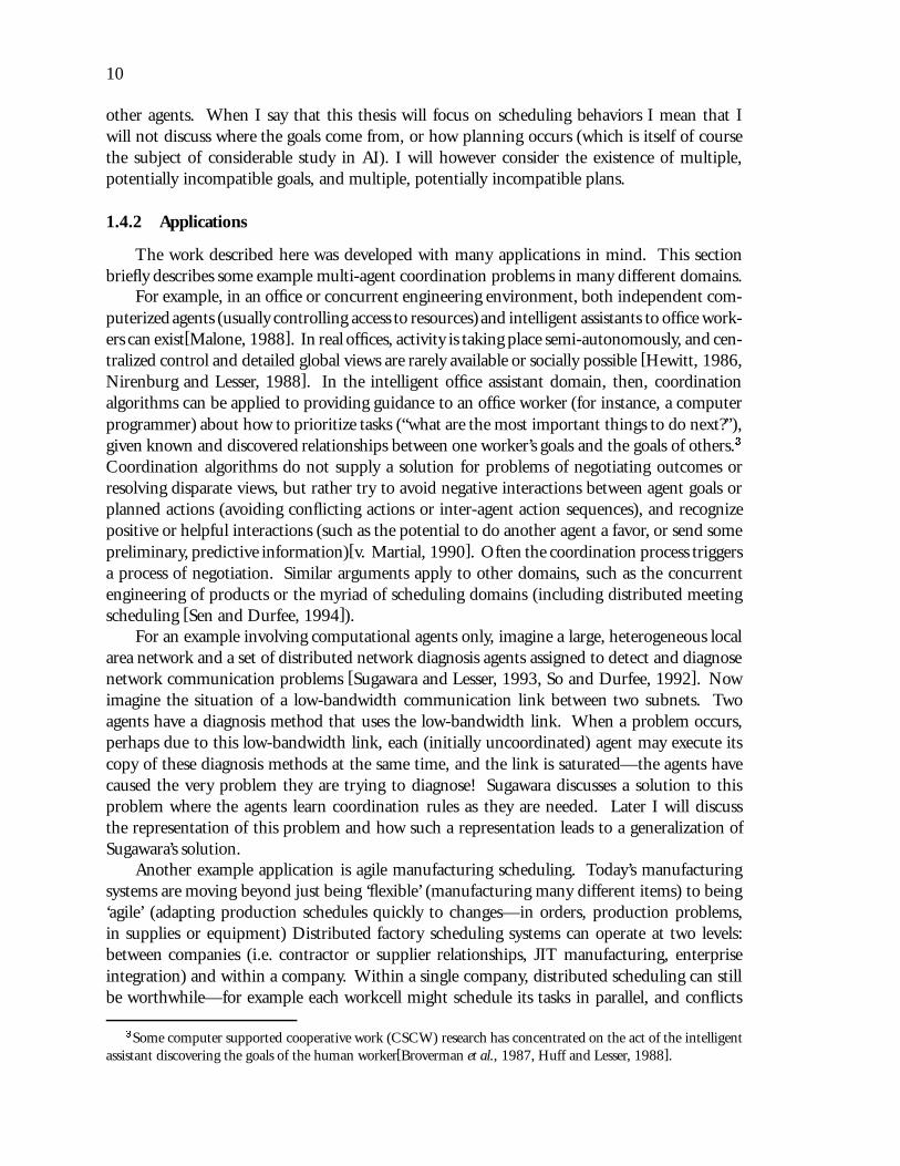
1.4.2 Applications

The work described here was developed with many applications in mind. This sectionbriefly describes some example multi-agent coordination problems in many different domains.

For example, in an office or concurrent engineering environment, both independent com-puterized agents (usually controlling access to resources) and intelligent assistants to office work-ers can exist[Malone, 1988]. In real offices, activity is taking place semi-autonomously, and cen-tralized control and detailed global views are rarely available or socially possible [Hewitt, 1986,Nirenburg and Lesser, 1988]. In the intelligent office assistant domain, then, coordinationalgorithms can be applied to providing guidance to an office worker (for instance, a computerprogrammer) about how to prioritize tasks (“what are the most important things to do next?”),given known and discovered relationships between one worker’s goals and the goals of others.3

Coordination algorithms do not supply a solution for problems of negotiating outcomes orresolving disparate views, but rather try to avoid negative interactions between agent goals orplanned actions (avoiding conflicting actions or inter-agent action sequences), and recognizepositive or helpful interactions (such as the potential to do another agent a favor, or send somepreliminary, predictive information)[v. Martial, 1990]. Often the coordination process triggersa process of negotiation. Similar arguments apply to other domains, such as the concurrentengineering of products or the myriad of scheduling domains (including distributed meetingscheduling [Sen and Durfee, 1994]).

For an example involving computational agents only, imagine a large, heterogeneous localarea network and a set of distributed network diagnosis agents assigned to detect and diagnosenetwork communication problems [Sugawara and Lesser, 1993, So and Durfee, 1992]. Nowimagine the situation of a low-bandwidth communication link between two subnets. Twoagents have a diagnosis method that uses the low-bandwidth link. When a problem occurs,perhaps due to this low-bandwidth link, each (initially uncoordinated) agent may execute itscopy of these diagnosis methods at the same time, and the link is saturated—the agents havecaused the very problem they are trying to diagnose! Sugawara discusses a solution to thisproblem where the agents learn coordination rules as they are needed. Later I will discussthe representation of this problem and how such a representation leads to a generalization ofSugawara’s solution.

Another example application is agile manufacturing scheduling. Today’s manufacturingsystems are moving beyond just being ‘flexible’ (manufacturing many different items) to being‘agile’ (adapting production schedules quickly to changes—in orders, production problems,in supplies or equipment) Distributed factory scheduling systems can operate at two levels:between companies (i.e. contractor or supplier relationships, JIT manufacturing, enterpriseintegration) and within a company. Within a single company, distributed scheduling can stillbe worthwhile—for example each workcell might schedule its tasks in parallel, and conflicts

3Some computer supported cooperative work (CSCW) research has concentrated on the act of the intelligentassistant discovering the goals of the human worker[Broverman et al., 1987, Huff and Lesser, 1988].

11

that arise between workcells during the day (errors, equipment failures, faulty estimates) mightbe rescheduled as they happen (scheduling processes can also be developed to be resistant tosuch errors in the first place). How should workloads be shifted (rescheduled) when a failureoccurs? When a customer asks for a delivery date, can a much more accurate date be given byactually adding the potential order to the existing schedule (as a query) rather than giving aseat-of-the-pants estimate? [Sycara et al., 1991, Neiman et al., 1994]

Long-haul telephone switching networks are already sophisticated distributed statisticalcontrol applications. The basic problem is how to route calls from, for example, one sideof the country to another. When a switch becomes overloaded, neighboring switches needto route calls around the overloaded switch. Current solutions to this problem use statisticaltechniques to re-route calls and balance the load (based on local statistical information).However sometimes re-routing is not the correct solution. If, for example, the overloadedswitch is servicing a national call-in talk show, the rerouted calls that are for the talk showshould not be re-routed, but denied instead [Adler et al., 1989]. The implication is thatstatistical routing could be supplemented with a decision process that takes into accountsymbolic information about call content, or other types of non-local information.

Distributed delivery tasks are another example application [Sandholm, 1993, Durfee andMontgomery, 1991]. For example (from TRACONET), requests for pick-up and delivery atarbitrary locations come into various regional trucking centers. Given the particular deliveriesbeing made, the number of trucks, etc., often it is worthwhile (because of lower mileage) toexchange jobs with other centers (both centers ending up better off in a distributed search forPareto-optimality). Such coordination processes can be useful even between different truckingcompanies (a situation where a centralized scheduler would not be appropriate).

Coordination behaviors in distributed sensor network (DSN) applications like the Dis-tributed Vehicle Monitoring Testbed (DVMT) will be discussed in great detail in this thesis.To state the problem briefly, several agents with physically distributed sensors have the taskof tracking vehicles moving through the combined sensed area. Coordination opportunitiesinclude avoiding redundant work in areas where the sensors overlap, balancing the processingload, and providing helpful results when some sensors are faulty or the data is open to manypossible interpretations.

Distributed information gathering applications might look something like the following:The original user query would be transformed into set of agents, each with their own plans forgathering information, where some plan elements must deal with the coordination of activitiesand construction of the final query response. Agents could be assigned to concurrently pursuedifferent sources to answer different aspects of the query or to make use of alternative typesof sources (e.g., text vs. images) to generate a more comprehensive answer. The agents wouldproceed to work in a distributed,asynchronous fashion, but there may be a need for coordinationamong the agents. For example, the results of work by one agent may suggest the need forsome of the existing agents to gather additional information from their sources or use alternatesources, or the results might suggest the need for additional agents. The agents must alsodeal with uncertainties about the availability of sources and the workload associated with thesources, which may require a new division of tasks among the agents [Carver, 1994].

Computational organization design tools use computer modeling of coordination. Exam-ple work includes the Virtual Design Team simulator for civil engineering projects [Levitt etal., 1994], designing organizations for decision-making under stress [Lin and Carley, 1993],

12

the Business Process Handbook project [Malone et al., 1993], computer-based modeling ofsoftware engineering processes [Mi and Scacchi, 1990], the ACTION system for re-engineeringelectronic small-parts manufacturing organizations [Hulthage, 1994], and the work I willdescribe in this dissertation on modeling computational agent environments and designingnew coordination mechanisms.

1.5 Chapter Summary

A coordination problem consists of some environment, the occurrence of episodes withinthat environment, and the structure of tasks within the episodes. Activities are related to oneanother so that the choice and temporal ordering of the activities affects some performancecriteria. Agents may have incomplete views, task structures may change during problem solving,and agents are uncertain about the outcomes of their actions.

The basic problem which this dissertation addresses is how to state coordination problemsin a formal, domain-independent way. Our approach is to first develop a framework, TÆMS,to directly represent the salient features of a computational task environment. The uniquefeatures of TÆMS include that it quantitatively represents complex task interrelationships, andit divides a task environment model into generative, objective, and subjective levels. We thenextend a standard methodology to use the framework and apply it to the first published analysis,explanation, and prediction of agent performance in a distributed sensor network problem.We predict the effect of adding more agents, changing the relative cost of communication andcomputation, and changing how the agents are organized. Finally, we show how coordinationmechanisms can be designed to respond to particular features of the task environment structureby developing the Generalized Partial Global Planning (GPGP) family of algorithms. GPGPis a cooperative (team-oriented) coordination component that is unique because it is built ofmodular mechanisms that work in conjunction with, but do not replace, a fully functionalagent with a local scheduler. GPGP differs from other previous approaches in that it is nottied to a single domain, it allows agent heterogeneity, it exchanges less global information,it communicates at multiple levels of abstraction, and it allows the use of a separate localscheduling component. We prove that GPGP can be adapted to different domains, and learnwhat its performance is through simulation in conjunction with a heuristic real-time localscheduler and randomly generated abstract task environments.

The next chapter, Chapter 3, will present and discuss the TÆMS modeling framework indetail. Chapter 4 will present the analysis and verification of a model of a simple distributedsensor network environment, and Chapters 5 and 6 will present and verify the GPGP familyof cooperative coordination algorithms. Chapter 2 will discuss other work related to thisdissertation. Finally, Chapter 7 summarizes this work and points out the many short- andlong-term research pathways that arise from it.

C H A P T E R 2

RELATED RESEARCH

There is no best way to organize. Any way of organizing is not equally effective.

— Jay Galbraith, 1973

Our intent is to show that overly specialized organizational structures allow effectivenetwork performance in particular problem-solving situations, but that no suchorganization is appropriate in all situations.

— Durfee, Lesser, and Corkill, 1987

We also expected different dimensions to resolve [coordination] conflicts better indifferent situations. : : :We also expected each dimension to be applicable at differentlevels of detail, with varying results.

— Durfee and Montgomery, 1991

The first subsection discusses briefly the reasoning behind the task environment modelingapproach. The next two sections discuss the questions of ‘What is a coordination behavior?’ and‘How does the task environment affect coordination behavior?’. These sections will concentrate onthe organizational theory literature, because it is probably much less well known to computerscientists. Afterwards I’ll return to the Distributed AI conceptual view. General backgroundon Distributed AI has been published by the author in [Decker, 1987]. An introduction toDistributed AI testbeds was published by the author in [Decker, 1994a].

2.1 Task Environments

The reason we have built a framework for task environment modeling is rooted in thedesire to produce general theories in AI [Cohen, 1991, Cohen, 1992]. At the very least, ourframework provides a featural characterization and a concrete, meaningful language with whichto state correlations, causal explanations, and other forms of theories.

The form of a task environment model in our framework is drawn from several sources.First and foremost is our own and others work in the DVMT and similar domain environmentsimulators [Corkill and Lesser, 1983, Lesser and Corkill, 1983, Durfee and Lesser, 1987,Durfee et al., 1987, Cohen et al., 1989, Decker et al., 1990, Carver et al., 1991, Decker et al.,1991, Decker et al., 1992]. It is from this work that the basic model form—the execution ofinterrelated tasks—is taken.

One possible form might have been to create a simulator (ala Tileworld [Pollack andRinguette, 1990]), but it would be very hard to state good featural characterizations using asimulator. The second input to the form of the model is the mathematically formal workin DAI (for example, [Genesereth et al., 1986, Rosenschein and Genesereth, 1985, Malone,

14

1987, Cohen and Levesque, 1990, Gmytrasiewicz et al., 1991]). There was no reason thatthe complexities that occur in our earlier DVMT simulation work could not be given clearsemantics.

The existing formalisms, however, universally eschew much complexity to allow foroptimal analyses to be carried through. For example, Malone [Malone, 1987] formalizesclassical organizational and economic coordination devices (i.e., product hierarchies, functionalhierarchies, centralized and decentralized markets) and analyzes them using queuing theory.This analysis is oriented mostly toward task assignment (i.e., how much time does it taketo assign and execute a task, how much communication is needed, and how vulnerable isthe structure to a failure of some component). Tasks are assumed to be independent withexponential arrival times, and all tasks must be completed. The work of Cohen and Levesque(for example, [Cohen and Levesque, 1990]) makes few assumptions about the environment:

“: : :we model individual agents as situated in a dynamic, multi-agent world, aspossessing neither complete nor correct beliefs about the world or the other agents,as having changeable goals and failable actions, and as subject to interruption fromexternal events.” [Levesque et al., 1990]

Instead, Cohen and Levesque concentrate on giving formal definitions and semantics to termssuch as ‘intention’, ‘commitment’ and ‘joint intention’—although they “: : :do not explorehow these ideas can be applied in computational systems that reason about action: : : ”. In[Genesereth et al., 1986, Rosenschein and Genesereth, 1985, Gmytrasiewicz et al., 1991],computationally tractable decision processes are worked out for particular environmentalsituations, such as the prisoner’s dilemma and other game theoretical environments. Oftengame theoretical models of environments [Luce and Raiffa, 1958] are unappealing becausethey assume a great deal of certain, static knowledge about the structure of the environment.Of course this work is still very useful in providing bounds and comparisons to more complexsituations.

The second desired characteristic of our task environment modeling framework is, then,to provide clear semantics but not to force the person doing the modeling to simplify thingsjust so that an optimal solution can be found. In this way we hope to build richer and morerealistic models—but ones that are still undeniably simplifications of real problems. We willmake simplifications to allow analytical solutions to be derived (see the Prisoner’s Dilemmaexample in Section 2.4.5.4 and the DSN analysis in Chapter 4). We will also use simulationtechniques when we don’t make such simplifications (see Chapter 5).

The third input to the form of a task environment model was the desire to avoid theindividualistic agent-centered approaches that characterize most AI (which is probably fine)and DAI (which may not be so fine). The view that what you and I would both agree to callan ‘organization’ can be described as some sort of ‘larger’ individual agent is faulty [Allison,1971] (I’ll come back to this in the next subsection). This is the reason the task environmentmodel goes to considerable length to avoid formalizing, say, the mental structure of an agentinteracting with the environment. This perhaps stubborn feature of the model allows us toadapt to the individualistic semantics of Cohen, Rosenschein, or Shoham. What I mean bythis is that I can use an environment model I build in conjunction with one of these agentarchitectures to explore how those agents behave in that environment. I will, for example, usea fairly Shohamesque agent architecture to demonstrate GPGP in Chapter 5. Look back at the

15

quote from Cohen and Levesque: our modeling framework should provide such a dynamicworld of incorrect and incomplete beliefs, changeable goals, failable actions, and interruptions.We wish to allow the model to provide:

“: : : a fabric of knowledge, resources, and actions out of which agents actively andflexibly construct and reconstruct themselves by adding and subtracting resources andchanging agent-knowledge boundaries. It is the overall collection of problem solvingknowledge that is fixed—not the definition of agents.” [Gasser and Ishida, 1991]

This provides a potentially more open system and social perspective than is usual in DAIresearch [Hewitt, 1991, Gasser, 1991].

A final problem remains with the form of the model that I can only address as a “futuredirection”: that of the mutual construction of agents and their environment. The organizationof the world is not wholly dictated either by people individually or by their environments [Agre,1991, Latour, 1987].

2.1.1 Example Task Environments

For the purposes of discussion and illustration, several of the concepts in this chapter willrefer to two task environment simulators developed at the University of Massachusetts: theDVMT and Phoenix.

DVMT.

The Distributed Vehicle Monitoring Testbed (DVMT) [Lesser et al., 1987] simulates anetwork of vehicle monitoring nodes (agents), where each node is a problem solver that analyzesacoustically sensed data to identify, locate, and track patterns of vehicles moving through atwo dimensional space. Each problem-solving node is associated with a sensor or sensors.In the simulated domain environment, each vehicle generates sounds (at particular locationsand discrete times) that are described by a grammar in terms of signal groups, which are thendescribed in terms of low-level, detectable signal frequencies. We will be analyzing an abstractsimplification of this problem in Chapter 4.

Phoenix.

The Phoenix firefighting testbed [Cohen et al., 1989] is another domain simulator.Although not primarily a DAI testbed, it does have multiple agents (firebosses and bulldozers)operating semi-autonomously in a highly dynamic environment (a fairly complex fire simulationbased on weather conditions, Yellowstone National Park’s physical features, and firefighting dataof the burn rates of various land types). Some work has been done on coordinating multiplefirebosses [Moehlman et al., 1992] through negotiation over bulldozers considered as resources.

2.2 What is Coordination Behavior: The Social View

When beginning our consideration of how the environment affects coordination, I earlyon came across the following general problem:

16

Consider the difficulties facing the experimenter asking the following question: “Whateffect does the environment have on learning ability”? This question meets all thecriteria of a problem and yet is stated in such a vague way that the investigator couldnot pinpoint what was to be investigated. The concepts of environment and learningability are vague. What environmental characteristics? Learning of what?

— An Experimental Psychology Textbook

This problem of conceptual vagueness can be considered yet another reason behind ourextensive mathematical modeling of the environment discussed in the previous section, andthe cautious set of basic agent behaviors (execution, communication, information gathering).This is also the reason for focusing our causal model on the production of local schedulingconstraints (a basic, observable, measurable output that may be based on other behavior suchas communication, negotiation, organization, etc.)

In this section I will first discuss how researchersview coordination behavior, and then I willdiscuss in what way other researchers have proposed that the environment has an effect on suchcoordination behavior. Here I will cover the views of social/organizational researchers. Untilrecently, DAI has had a very impoverished view of coordination, often equating coordinationbehavior merely with the communication of messages, thus it is profitable to be inclusive aboutother’s ideas. I will return to the DAI perspective later in this chapter (Section 2.4).

The recurrent problem in sociology is to conceive of corporate organization, and studyit, in ways that do not anthropomorphize it and do not reduce it to the behavior ofindividuals or of human aggregates.

— Guy E. Swanson, The Tasks of Sociology

Several schools of thought in sociology and management science have their own views ofcoordination behavior: the rational systems school, the natural and institutional schools, theopen systems school, the economic systems school. These researchers often separate normative(expected or predicted assuming no outside influences) and observed behaviors. The nextseveral sections will briefly summarize the point of view of each school on what is coordinationbehavior.

2.2.1 What is Coordination Behavior: Rational Systems

In the rational systems view the most important features of organizations are whattheir specific goals are and what their normative structure is. Organizational activities andinteractions are coordinated to achieve these goals; the goals themselves are explicit and includecriteria for choosing the best activity. Agents interact explicitly according to the rules ofthe normative structure, which describes roles and interactions separately from the personalattributes of the agents occupying those roles [Scott, 1987].

The fundamental rational systems normative structure is the bureaucracy. The term hasa technical sense, apart from its pejorative colloquial use [Perrow, 1986, Weber, 1947]. Thisnormative structure promotes several types of coordination behaviors:

Rules and Regulations: The creation and adherence to rules and regulations is one coordina-tion behavior observed by rational-legal bureaucracies. Rules and regulations apply toindividual agents or subgroups. Their purpose is to:

17

� Justify decisions or actions (especially unpleasant ones)

� Control interactions with the environment

Standardization: The creation and use of standards is a special case of regulations put intoplace to reduce uncertainty, both within and organization and in its interactions withthe environment.

Hierarchy: Hierarchies specify where knowledge, skills and other resources lie, and thus containcommunication information. Most importantly, hierarchies outline the nominal powerstructure — who makes which decisions. Constructing or accessing hierarchies is acoordination behavior.

Specialization: individuals or groups with tightly coupled communication requirements areoften departmentalized. This functional division is another coordination behavior.

There exists a natural tension between hierarchy and task specialization. A hierarchygroups together routinely related tasks, but in non-routine situations may be a hindranceto coordination of widely separated groups. The modern solution, from the rational opensystems view, is to create special task groups that set apart from the routine hierarchy fornon-routine situations, transferring the appropriate decision making power to a closer point.If the non-routine situation persists, it may result in a permanent change in the organization.Thus the creation of special task groups is another coordination behavior (although it wouldbe properly classified as a ‘rational open system’ approach).

2.2.2 What is Coordination Behavior: Natural Systems and Institutions

The natural systems, human relations, and institutional views have in common the factthat they are all reactions to the the rational systems view. They point out that organizationsare made up of people, not automatons, and the rational systems view does not take thatsufficiently into account.

Of course, for our purposes of studying coordination in distributed problem solvingsystems, organizational actors are (often) automatons! Thus these points-of-view do notprovide me with the easy insights that the rational (and rational open) systems views do. I coverthese views here for the light they may shed on mixed human-computer coordination behavior.Furthermore, some amount of “irrationality” may in fact facilitate effective problem solving[Lesser 1991, personal communication]. For example, the node skepticism idea [Corkilland Lesser, 1983] advocates indirect organizational structuring, which allows each agent todecide whether to accept its organizational role. A node may choose to be guided more bythe proposed organizational structure (to be a “company node”) or may decide that its owninterests are more important (an “entrepreneurial node”). This freedom is important since theorganizational structuring was done with uncertain and incomplete information and thereforemay be incorrect. A certain fraction of nodes with each ‘personality’ may result in a morerobust organization in the face of changing environments, an observation that has been madein reference to colonies of honey bees [Reed and Lesser, 1980].

A common tenet of these views is the concept of structural-functionalism, i.e., organizationalstructures can be explained by examining their functions, and certain functions imply certainstructures; however [Perrow, 1986]:

18

The explanation for organizational behavior is not primarily in the formal structureof the organization, the announcements of goals and purposes, the outputs of goods andservices. It lies largely in the myriad subterranean processes of informal groups, conflictsbetween groups, recruitment policies, dependencies on outside groups and constituencies,the striving for prestige, community values,the local community power structure, andlegal institutions.

Institutional organization theory [Meyer and Scott, 1983] tries to explain the actions oforganizations as attempts to manage their perceived, external image so as to secure supportfrom external sources. Thus an organization will prefer to pattern its structure and operationsas a copy of other institutions rather than attempting to maximize its efficiency or some otherrational-systems-view measurement. For example, Meyer and Rowan [Meyer and Rowan,1977] argued that when Congress enacted affirmative action legislation, many organizationscreated an “Office of Equal Opportunity” as a symbolic response—no genuine response wasintended.

A primary coordination behavior observed by natural systems and institutional researchersis the construction and use of informal channels [Chisholm, 1989], i.e., communicationschannels that neither exist in the formal hierarchy, nor were created by formal mechanisms.These communication channels can exist both within an organization and between parts of theorganization and the environment.

2.2.3 What is Coordination Behavior: Open Systems

The original conceptions of the rational and natural systems views tended to view organiza-tions in isolation from their environments, with a static set of participants and goals (includingthe survival of the organization itself). The open systems point of view stresses the environmentthat the organization operates in — how do participants come to the organization and why dothey become a part? How does the organization obtain resources (including physical resources,agents, knowledge, and time) from the environment? Scott summarizes the open systemsdefinition as [Scott, 1987]: “organizations are coalitions of shifting interest groups that developgoals by negotiation; the structure of the coalition, its activities, and its outcomes are stronglyinfluenced by environmental factors.”

The open systems view of coordination behaviors includes:

� Negotiation and adoption of shared goals by groups and individuals. This is the mostcomplex coordination behavior, often underlying many of the others mentioned here1.

� The construction and execution of multi-agent actions (plans).

1Negotiating coordination strategies include contracting (of course), bargaining, and ‘co-optation’. The lastone is coordination by representation. Suppose I have two large CDPS systems that are separate, but have strongmutual coordination relationships in some overlapping area. One coordinating activity is to simply involve arepresentative from each organization in the decision process of the other — rather than for Agent A to try totransmit all of its plans to B, simply ask A to make a choice from B’s palette of choices. A will use it’s owninformation and decision procedure, and B can factor A’s decision in with it’s own view. Other styles of thisstrategy can exist between large networks of agents where the agents themselves can be traded or merged into newpermanent or temporary organizations.

19

� The commitment behavior defined by Gerson [Gerson, 1976]. A commitment is a de-pendency, or “side-bet”, relating initially unrelated negotiations or potential negotiationsand their outcomes to those in the situation at hand. The commitment is a flow orconstraint on the flow of resources. For example a schedule is a time commitment, abudget a monetary commitment, loyalty is a commitment of solidarity.

� Power sharing — two mostly independent organizations may share seats on their boardsof directors, which is a coordination behavior. Delegation of authority is also in thiscategory of coordination behavior.

� Professionalization — some complex problems are solved by giving complete control toa single agent. This agent both makes decisions and executes tasks.

� Slack — creation of slack in resources (computational (‘satisficing’), informational(‘information buffers’), or physical (‘stockpiling’)) is a coordination behavior. It worksby reducing the need for tight coordination.

� Coding — preprocessing organizational inputs reduces uncertainty and complexity inthe environment, which in turn eliminates or simplifies other coordination behaviors.

� Forecasting or prediction is a typical coordination behavior if the environment allows it.

� Growth — especially forward or backward vertical integration [Perrow, 1986]. Again,usurping control over part of the environment can either eliminate or reduce the needfor coordination, and so certain types of growth can be viewed as coordination behavior.

2.2.4 What is Coordination Behavior: Economic Systems

The newest school of organizational theorists are, or are influenced by, economists. Thusthe driving force behind coordination behaviors of agents is the maximization of their individualutilities. This should not be too surprising, given the game theoretic approaches to DAI[Genesereth et al., 1986, Rosenschein and Genesereth, 1985, Gmytrasiewicz et al., 1991].While the detractors of these theories have strong arguments [Perrow, 1986], many of thearguments are based on natural systems views and are not as convincing when applied tocollectively engineered CDPS systems. The DAI work in this area has focussed on makingrational decisions when outcomes will be affected by what multiple agents do—this is really adifferent problem than the distributed scheduling problem addressed by GPGP.

These economic theories do not postulate new behaviors, but rather new explanations forexisting behaviors. The first, principal-agent theory, explains hierarchical organizational behaviorin exactly these terms—self-interested agents maximizing their individual utilities [Moe, 1984,Perrow, 1986]. The second, transaction costs economics, takes a more encompassing approachin explaining hierarchical organizational structures as arising from bounded rationality, uncer-tainty, and other features of the environment. I will explain these relationships in Section 2.3.

This section has briefly discussed a few perspectives on coordination behavior that donot originally come from the AI community. The purpose of this section was to get thereader thinking about the idea that there are many different coordination mechanisms andperspectives on these mechanisms. The next section will try to briefly summarize somenon-computational perspectives on the the relationship between the task environment andthese different coordination mechanisms. It is not an exhaustive list.

20

2.3 How Does the Environment Affect Coordination Behavior: The Social View

The social conception of the environment [Scott, 1987] is that no organization exists inisolation, but rather in a complex set of relationships with its environment. The environmentconstrains the types of participants that can make up an organization and includes what otherorganizations those participants belong to. The environment is the source of inputs to theorganization, the source of technologies2 with which to process those inputs, and the sinkfor organizational outputs. The things that are goals from the organizational point of vieware the specialized functions of the organization from the environment’s point of view. Thecomplexities of the environment are reflected in the complexities of the organization’s structure.Organizations and their environments are interdependent, and each can influence the other.

In characterizing the environment, one has to decide what level of analysis is appropri-ate. Perrow [Perrow, 1986] enumerates possible analyses at the individual, group, division,organization, inter-organizational, network, industrial, national, and world levels, to namea few. For our purposes in DAI, individual (i.e., an agent with a virtual single locus ofcontrol), organizational, and network analyses seem the most applicable. Network analysis isthe process of modeling the control and influence relationships arising from an organization.While the boundaries of a single organization, a hospital for example, are more-or-less clear(there are always boundary problems, however), the network of organizations that make up itsenvironment is large and fuzzy (including other hospitals, federal, state, and local governmentalagencies, labor unions, professional societies, support groups, etc.) Constructing a model of asingle organization without reference to the network it is part of is an error.

Another way to look at the interactions between units of study, and the levels above andbelow the units, is to think of the sources of inputs, the markets for outputs, the competitors,and the regulators [Scott, 1987]. One can then characterize the environment as a place whereresources are located, both physical and information. An organization can be dependent on aphysical resource, or have uncertainty because it lacks some information. Various sociologicalstudies have shown causal effects between certain variables and organizational dependence anduncertainty. Scott mentions the following (I’ve added my own examples using the DVMT andPhoenix (Section 2.1.1) which he may or may not agree with):

� Dimensions affecting dependency

Degree of munificence/scarcity: How easy are the resources to come by? Also calledenvironmental capacity. Phoenix has a limited number of bulldozers with which tofight fires, but a potentially unlimited amount of fireline can be built. Time can beconsidered a resource. The fixed DVMT sensors are limited resources.

Degree of concentration/dispersion: How are the resources spread out in the environ-ment? DVMT sensors are fixed, and evenly distributed. Vehicles can appearanywhere. Bulldozers can be moved anywhere, at the cost of time lost. Fire canappear almost anywhere.

Degree of coordination/non-coordination: Are the entities in the environment execut-ing orchestrated or structured actions? For example, in the DVMT, some vehicles

2Means for doing work. Machines, knowledge, and skills are technologies. This is a sociological term; computerscientists would probably use the term resources.

21

can be part of a single pattern, and act in a coordinated way with one another. Bycontrast, in Phoenix, multiple fires are uncoordinated (i.e., the fires don’t decideon a joint plan to burn an area) and independent.

� Dimensions affecting uncertainty

Degree of homogeneity/heterogeneity: How similar are the entities in the environmentto which the organization must relate? Also complexity, diversity. Vehicles havenoticeable differences. Bulldozers are all the same (although one can easily imaginethe addition of helicopters, and different types of bulldozers, etc.). Also, thehomo-/hetero- geneity of the terrain can lead to changes in the qualities of fires(see also “degree of stability/variability” below).

Degree of stability/variability: How quickly, (or, alternately, evenly) are the entities inthe environment changing? The DVMT has a very stable environment. ThePhoenix environment is more variable when one considers the changing winds andweather.

Degree of threat/security: Is the organization/entity under study vulnerable to its envi-ronment? Will “inefficiencies and errors by an organization result in its demise”[McKelvey, 1982]? The DVMT is secure; The Phoenix organization is secure butthe bulldozers are not.

Degree of interconnectedness/isolation: To how many, and how closely, is the entityunder study linked to other entities in the environment in a way that the otherentities can affect the one under study? Both the DVMT and Phoenix agents arepartially isolated from their environments, but fires can directly affect the firebossby destroying bulldozers. The intra-entity connections, between DVMT agents orbetween multiple Phoenix firebosses, are very strong.

Degree of coordination/uncoordination: This dimension effects uncertainty about theenvironment as well as dependence on environmental resources (that may becontrolled by other entities).

Scott notes that these independent variables (uncertainty and dependence) are orthogonal.For example, if the entities in the environment are highly coordinated, it decreases environmen-tal uncertainty (they are more predictable) but may increase dependence (because it reducesthe number of independently available resource locations).

Another point to keep in mind when analyzing an environment, which should be clearfrom the proceeding discussion, is that the analysis of an environment is inextricably linkedto “: : : the organization, the cognitive work of its participants and their structure of attention,and its information system” and “the characteristics and goals of the organization [: : : ]each [organization] functions in a different domain”[Scott, 1987]. Or, in other words, theenvironment is linked to the agent (organization) architecture and the desired agent (organization)behaviors3[Cohen et al., 1989]. Scott points out the difference between what the characteristics

3One of the reasons that the Partial Global Planning coordination algorithm works is goal reinforcement —when a remote goal is equivalent to, or is compatible with, local goals, then the combined goal is rated highly;this happens to be a good thing in the DVMT domain and environment[Decker and Lesser, 1990]. To the extentthat one believes goal reinforcement is true in the world at large, the above similarity is encouraging.

22

of the environment are and how the entities perceive those environmental characteristics.Perceptions can be used to predict entity actions or outputs (goods, services, problem solutions),but unperceived characteristics can still affect outcomes, which are the results of the interactionbetween outputs and the environment. What agents don’t know can hurt (or help) them[Scott,1987]. Scott (and Perrow) demonstrate that market perceptions held by recording industryexecutives can predict who will get a recording contract, but not how well the record will sell.

An illustrative example of outcome vs. outputs in the DVMT is the case of the ghost track.A ghost track is a weakly sensed vehicle track caused by sonic reflections from a real vehicle, andoccurring nearby. A ghost track is coordinated with the track of the vehicle that it is a ghostof; this fact was true in early DVMT environments. However, the DVMT had no knowledgeabout ghost tracks; it did not perceive the coordination between ghost tracks and vehicle tracks;it was blind to that characteristic of the environment.

2.3.1 How Does the Environment Affect Coordination Behavior: Contingency Theory

One theme of this dissertation is the development of a method of designing coordinationalgorithms for CDPS systems. Some very special coordination algorithms have provablygood behavior under restrictive conditions [Rosenschein and Genesereth, 1985, Zlotkin andRosenschein, 1990]. Some algorithms claim much greater generality but have a large numberof parameters (PGP has 12 cooperation parameters used in the hill-climbing task reorderingalgorithm, the meta-level organization chosen, and the time-cushion parameter used in thepredictability and responsiveness experiments) or are known or believed not to perform wellin certain classes of situations (i.e., heterogeneous, dynamic, and ‘real-time’ situations [Deckerand Lesser, 1990]). In any case, there is to this date no coordination algorithm that is trulygeneral.

If we are interested in designing coordination algorithms for intelligent agents, it only makessense to look at the design of coordination algorithms for humans. Human organizationaldesign was once (before the ’60s) faced with myriad designs that all tried to be good for allsituations. It was then noticed that very different organizational designs flourished in industrieswith different technologies (problem solving methods & knowledge), and in industries whereexternal change took place more quickly or more slowly.

It was clear that there was not a single good organizational structure, but it remained tobe shown that the structure mattered. Perhaps one would be as good as another. Lawrenceand Lorsch [Lawrence and Lorsch, 1967] built a model (using the aforementioned studies andtheir own studies) that relates uncertainty in the environment to differentiation and integrationin the organizational structure. This model and its elaborations are called contingency theory.Lawrence and Lorsch define their independent and dependent variables as follows:

2.3.1.1 Definitions

To apply the definitions below, you should have a clear level in mind. An organizationis made up of parts. For example, the organization “U.S. Government” is composed of an“executive branch”, “legislative branch”, and “judicial branch” (the parts). Obviously parts canalso be organizations themselves.

The organization “General Electric” comprises “the service businesses”, the “aerospacebusinesses” and “the core businesses”. Note that a level of analysis is not necessarily the same,

23

in human organizations, as the org chart. There are a lot of reasons for this that I doubt anyoneis interested in : : : but the formal org chart can be a starting place.

The organization “DVMT” comprises “DVMT agents”. DVMT agents comprise a controlcomponent and a domain component. Each of these is composed of knowledge sources.Phoenix is composed of a fireboss, a group of bulldozers, a group of watchtowers, and a groupof helicopters (?). Each group comprises individuals.

In the set of studies from which this was derived, there are a set of numerical measuresassociated with the definitions. I can’t see these as being too useful, since they are orientedtowards the business world. If this is a useful theory, I should be able to build models of oursystems with it, but I will need a different operationalization of the variables. For example, Iwould have tremendous difficulty trying to determine the change in profits the DVMT madebefore and after the Partial Global Planning mechanisms, but I can easily come up with otheroperationalizations of performance, like “on the same test suite, the new DVMT found X%more solutions, was Y% more confident in them, and did it executing Z% fewer KSIs.”

So I will give the original definitions in order to be concrete, but encourage you tothink of how the concepts transfer. The data used to develop this theory came from severalenvironments, but the examples I give are from the plastics environment. An organizationin the plastics environment comprises research, applied research, marketing, and productionparts. Each part interacts with its own subenvironment in the plastics industry.

Environmental Uncertainty: Environmental uncertainty can be measured by three factors:

1. Clarity or uncertainty associated with inputs or measurements. For example,the environment associated with the research part of organizations in the plasticsindustry has a higher degree of uncertainty associated with its inputs than any otherpart of an organization in the plastics industry.

In the DVMT world, I would say that a DVMT agent with a faulty sensor has highuncertainty associated with its inputs or measurements.

2. Uncertainty associated with causal relationships. For example, in the plasticsindustry, “the performance characteristics required by the customer are well known,but as far as research is concerned,you might as well be asking for the perfect plastic.”

In DVMT world, there are questions like ‘do all ducks attack fish?’, etc. There is agreat deal of uncertainty associated with the causal and deductive relationships inthe DVMT, but it is the same for each agent.

3. Time span of definitive feedback after making a decision. In the plastics industry,it may be years before a research program pays off or pans out, but errors inplastics production are usually noticed (and corrected) within a week. Researchand production are parts of organizations in the plastics industry.

In the DVMT I can also measure the amount of time between when a decision ismade (i.e., a KS is run) and when I know if it is a correct one. However, for thepurposes of Theorem 1.1 below, it is sufficient to note that this feedback time isnot significantly different for each agent.

Degree of Differentiation: Two organizational parts are considered to be more differentiatedthe more they differ along the following 3 dimensions:

24

1. Formality or rigidity of their structures (are they unorganized, adaptable, or rigid).For example, the production part of one plastics organization was very formal andrigid because it had a deep hierarchy of managers and frequently reviewed theirperformance and rarely allowed the lines of authority to be breached. The sameplastics organization had a research lab that had only a handful of lab managersto whom all scientists, engineers, and support staff reported to. The researchlab encouraged (by decree and monetary incentives) collaboration between staffmembers. Each DVMT agent has the same internal structure.

2. Time-frame orientations (do they solve problems over the course of minutes,hours, days). In one plastics organization, production and sales were concernedwith problems and schedules that often lasted less than a month, while researchoften planned projects lasting years. Each DVMT agent has the same time-frameorientation.

3. Attention to high-level goals (are they equally interested in the quality of thesolution, the solution cost, efficiency, utilization). This was simply a measure ofwhether the smallest studied parts of a part of an organization actually performed inaccordance with the organization’s stated goals for that part. The scoop in plastics,for example, was that low-level employees did, in fact, behave consistently withthe high-level goals except for research scientists, who seemed to have more of anorientation toward production and sales goals than could be assumed from thestated research goals. Each DVMT agent, by construction, attends to system goals.

A fourth dimension, interpersonal orientation, was also used as a sign of differentiation,but I had trouble operationalizing the concept. It was measured on a 2 unit scale: a or-ganizational part was either “task-oriented” (research) or “socially oriented” (marketing).

Required Integration: For a given partitioning of an organization into parts, some amountof collaboration, to achieve unity of effort, will be required between any two parts bythe overall environment under which they operate. This can be measured on a binaryscale—either the linkage is critical or it is routine. For example, in the environment of theplastics industry, there is a critical link between production and research (manufacturinginnovative products), and another between sales and research (finding customers forinnovative ideas and finding ways to create what the customers want). The link betweensales and production, or sales and applied research, is routine. In a different environment,say the container manufacturing industry, the same parts are not critically linked in thesame way. Critical linkages in the container industry occur between production and sales(delivery constraints) and production and research (quality control problems)

The classic DVMT environment places critical linkages between agents whose sensorareas are spatially overlapping, because of the need to (1) reinforce the discovery of atrack and (2) look for other parts of a multi-vehicle pattern.

Effective Organization: Effectiveness can be measured by technical performance, for example,a business can be ranked by its change in profits, sales volume, and new productsintroduced over the past 5 years.

Incarnations of the DVMT have been ranked by quality of solution, number of KSIsexecuted, and (probably unfortunately) CPU time and memory usage.

25

The model can then be expressed by the following 3 propositions:

1. In effective organizations, the degree of differentiation between the parts of the organi-zation varies proportionally with the diversity of uncertainty in the environments of theparts.

In other words, the more different the environments were (as measured by environmentaluncertainty) the more different the parts of the organization in those environments were,for effective organizations. Poorly performing organizations tended to either force all partsof the organization to remain undifferentiated in the face of environmental differences,or to allow differentiation where the environment did not require it.

Analyzing at the agent level, the classic DVMT, while its environment is uncertain, isnot diverse (not different for each part, in this case an agent). The model predicts thatDVMT agents should be undifferentiated, and explains this by pointing out that thesubenvironment of each individual DVMT agent has an equal amount of uncertaintypresent (measured by uncertainty of inputs, uncertainty in causal relationships, and timespans of feedback on agent decisions).

2. Effective organizations achieve better integration at the critical environmental linkagesthan less effective organizations.

For business organizations, the quality of integration was measured using surveys of themanagement. For example, “Relations between these two units are: (1) Sound — fullunity of effort is achieved : : : (4) Average — sound enough to get by even though thereare many problems achieving joint effort : : : (7) Couldn’t be worse — bad relations —serious problems exist that are not being solved”

One way to measure the quality of integration between DVMT agents, off the top ofmy head, would be to measure the percentage of possible joint solutions that are actuallydiscovered by a pair of spatially adjacent (i.e., critically linked) agents. The modelpredicts that the DVMT should discover a greater percentage of joint solutions betweenspatially adjacent agents than between spatially non-adjacent agents.

3. I’ll break this into two parts:

[A] There is an inverse relationship between integration and differentiation.

[B] When parts of an organization are both highly differentiated and highlyinterdependent it is necessary for the organization to develop more compli-cated mechanisms for achieving integration between them (if the organizationis to be effective).

The relationship [A] was discovered by pairwise comparison of organizational parts.For each pair, measure the amount of differentiation by the definition above. Nowmeasure the quality of integration actually achieved as described in Theorem 1.2. For allorganizations in all environments, the more differentiated the parts were, the lower thequality of integration between the parts.

The relationship [B] is discovered by looking at all organizations operating in the sameenvironment. The better the measured performance of the organization, the higherthe quality of integration. Thus high-performing organizations achieved high quality

26

integration even when highly differentiated. The rest of this and many other studiesgoes on to explore the mechanisms that these organizations used to achieve high qualityintegration between highly differentiated organizational parts.Part [A] predicts for the DVMT that its undifferentiated agents should all have the sameamount of resources devoted to integration.Part [B] doesn’t make a prediction for the DVMT, which is undifferentiated.

These are weak conclusions about the DVMT, and are mostly meant for illustrative purposes.The important point is that Lawrence and Lorsch’s work shows that:

1. not only was there no single good structure,

2. but that the choice of structure really did matter.

Galbraith [Galbraith, 1977] further illuminated this model by examining why uncertaintyin the environment should be a key independent variable. To Lawrence and Lorsch’s correlationhe added the following causal link:

The greater the amount of uncertainty of the task, the greater the amount of informationthat has to be processed between decision makers during its execution. If the task iswell understood prior to performing it, much of the activity can be preplanned. Ifit is not understood, then during the actual execution of the task more knowledge isacquired which leads to changes in resource allocations, schedules, and priorities. Allthese changes require information processing during task performance.

Thus the correlations observed by Lawrence and Lorsch can be explained by strategies toincrease the ability of an organization to preplan activities, increase flexibility to adapt in theface of not being able to preplan, and decreasing the level of performance required to solve theproblem.

2.3.2 How Does the Environment Affect Coordination Behavior: Information Processing

In newer work [Stinchcombe, 1990], Stinchcombe returns to the structure of the uncer-tainties facing economic organizations that is the basis of contingency theory (and arguablya progenitor of transaction costs economics, below [Padgett, 1992]). Organizations growtoward, and structure themselves around, sources of information important to them. An actualmechanism is postulated: the resulting structures are not so much a result of self-consciousrational choice, or unintended environmental selection4, but trial and error learning. Theinformation toward which an organization grows is not so much that which is used to forecastor predict the future, but rather information as news, information about particular outcomesthat indicate with some certainty how the future is going to be, in some way important to theorganization:

I propose that information about the uncertain future becomes progressively available indistinct social locations [: : : ] What resolves the uncertainty of [agents] is the earliestavailable information that will show what direction the [agent] ought to be goingbecause of the way the future of the world is, evidently, turning out [Stinchcombe,1990].

4Another popular organizational model I have not talked about in detail is that of ‘natural selection’, or the‘population-ecology model’ [Perrow, 1986].

27

2.3.3 How Does the Environment Affect Coordination Behavior: Principal-Agent Theoryand Transaction Costs Economics

Why do hierarchical organizations exist? From the DAI perspective,why aren’t contract net-style protocols all we need for DAI coordination problem solving? Both principal-agent theoryand transaction cost economics answer this question by denying the benevolent agent assump-tion [Rosenschein and Genesereth, 1985, Genesereth et al., 1986, Zlotkin and Rosenschein,1990] (again, from the DAI perspective). We will illustrate this with examples drawn from ahypothetical contract-net style system. These illustrations are drawn from [Williamson, 1975,Moe, 1984, Perrow, 1986, Stinchcombe, 1990], although of course none of these authors arereferring to DAI systems!

First, imagine a contract net agent putting a task to bid without the benevolent agentassumption. In such a system there would have to be some utility, or ‘reward’, for an agentto accept a task—probably the bid specification would indicate the amount of the reward—otherwise why would an agent ever accept a task?. Imagine that there are many agents capableof accepting the task, but that they are not all equally capable. The agents examining thebid specification know just how capable they are in accomplishing the specified task, but thecontracting agent cannot know these capabilities as well (without spending too many resources).For any given level of reward, some agents that are very capable will find the reward offeredinsufficient for them to take on the task. Other agents will find the reward generous for theirmeager capabilities, and thus eagerly accept the contract. Thus a situation referred to by theabstruse term adverse selection occurs, where the best agents for a task definitely do not bid onit, while the worst agents definitely do. Such things happen all the time in the real world,for example when hiring employees (“With all my experience and education, I’m worth muchmore than you are offering”), or when selling insurance (“I can’t believe these low rates. Theymust not have found out about our string of equipment fires,” thinks Springfield nuclear plantowner Mr. Burns on The Simpsons).

The problem of adverse selection can be mitigated somewhat by designing jobs for thecommon denominator—you don’t have to have the best, just the average for some packageof skills. Perrow points out that the adverse selection problem, especially with employmentcontracts, can run both ways (i.e., the individual doesn’t really know exactly what their new jobwill entail (and thus not really how capable they are); how awful their new working conditionswill be; how many times grad student fees, suspiciously not covered by their waiver, will triple,etc.)

A similar problem occurs after the contract starts. The task that was just contracted outis very complex—the result will have to be judged on a multiple criteria basis, such as on itscertainty, precision, and completeness. Each of these terms will have to be operationalized, andprobably watered down to a number in the process. The contracting agent does not have theresources to constantly monitor progress of the other agent, except perhaps for a few progressreports along the way. Since the agent is judged by this set of simpler criteria, rather than thetrue, hard to specify, original goal, what is to keep the contractor agent from doing as little aspossible, orienting its work to these secondary criteria rather than the original goal and thensleeping the rest of the day (or, perhaps for computers, moonlighting with other contracts thatwill also be done just barely to specification)? The recondite term for this situation is moralhazard. In the real world, after getting hired, the employee does as little as possible (‘shirking’),and what little they do is oriented toward how they are evaluated by management (think Homer

28

Simpson); after getting fire insurance, there’s no real reason to practice fire safety at the plantsince it probably won’t burn down anyway.

In both cases, there is uncertainty present—an ‘ informational asymmetry ’ between theagents involved.

The solution, incredibly enough, is capitalism!

— Charles Perrow, Complex Organizations

2.3.3.1 Principal-agent Theory

Principal-agent theory uses moral hazard (shirking) as the basis of the existence of hi-erarchical organization. Let us assume we have several agents who work together to trackvehicles, and they gain some global utility for their results. How do they divide up the rewards?Without the benevolent agent assumption, they cannot trust each other to tell the truth abouttheir individual efforts. “Precisely because of the complex interdependence of tasks” [Moe,1984] and the processing distance between the sensor inputs and the final tracks, it is hardor impossible to objectively determine each individual agent’s contribution. If the agents justsplit things up equally, each agent will bear its own costs and only get part of the reward—butif the agent shirks, the savings accrue only to it, while the reduced reward will be split amongall the agents. Thus it may be only rational for the agents to shirk. Depending on the exactcosts of work to each agent and the benefits accrued with and without shirking, the situationcan be viewed similarly to a multi-way Prisoner’s Dilemma, where the defector(s) cannot bepinpointed.

The principal-agent theoretical solution is for the agents to hire a principal which willspend its computational resources to monitor the agents, determining their individual effortsand safeguarding against shirking. The principal will allocate rewards to each agent appropriatewith their effort, and is given the ability to fire and hire new agents to get rid of shirkers.But how do you keep the monitor from shirking? By giving the principal the excess rewards(residuals) left over after each agent gets its share. The principal agent theorists sternly assertthat the resulting arrangement is not any type of ‘authority’ relationship, but more like a set ofspot contracts entered into willingly and rationally by all the parties involved.

This type of analysis can be applied to employee / employer relationships, management /stockholder relationships, and even politician / bureaucrat or citizen / politician (as discussedby Moe, but with the idea of a ‘residual’ redefined). The criticisms also abound, rangingfrom simple ones about the exact optimal form for a specific environment (should the agentsalso get part of the residual? could the principal position be rotated among the agents?), toPerrow’s vehement attack (basically, the model suffers from the wildly unrealistic assumptions ofneoclassical economics; that agents can always leave the principal without cost, and principalsfire and hire agents without cost; that it assumes that not all principals will cheat, bringing thesystem to a stable point where the principals get everything and the agents little; that authorityor unequal possession of power does not effect the model; etc.) Nilakant and Rao [Nilakant andRao, 1994] argue that by concentrating on adverse selection, moral hazard, and randomnessas the primary contributors to uncertainty in performance outcomes, principal-agent theoryoverlooks two critical sources of uncertainty in outcomes:

� incomplete knowledge about the relationship between effort and outcome

29

� lack of agreement about the measurement of effort, P-A theory preferring to measureonly quantity of effort, and not quality or type of effort.

Nilikant and Rao also argue that principal-agent theory ignores facilitative effort, where anagent does not directly effect the outcome.

In the beginning, there were markets.

— Oliver Williamson, Markets and Hierarchies

2.3.3.2 Transaction Costs Economics

Williamson’s transaction costs approach [Williamson, 1975] combines microeconomictheory with traditional organizational concerns such as bounded rationality and environmentaluncertainty. Again, the question being answered is why hierarchical organizations exist—Williamson answers this by showing the conditions under which the open-ended contractualtransactions identified with hierarchical organization are more efficient than short- (‘spot’)or long-term market transactions (and thus rationally preferred). Under this approach,organizational boundaries are not fixed, but rather arise from linkages between distinct featuresof the task environment and the agents. The approach has gained much support because ofits simple explanations of exactly why and where big, vertically integrated firms will come intoexistence, and where small firms will operate through markets.

The first of these linkages is between environmental uncertainty/complexity and agentbounded rationality. As we have pointed out several times before, coordination is much simplerwithout the presence of environmental uncertainty, since complete rational decision makingis possible (i.e., cooperation without communication [Genesereth et al., 1986]). Imagine,for example, how Phoenix might have been structured in an environment with an unlimitedbulldozing service market if fires were easily predictable—make the certain projection, getthe price of a bulldozer from the market, and make the tradeoff computation between price-of-bulldozers and amount-of-land-burned. But of course the problem isn’t that simple; thePhoenix planner can not make a certain projection, or even a finite number of possiblecontingencies to specify in advance, a feature of both the intrinsic complexity of fire growth,the environmental uncertainties (wind speed and direction, for instance), and the boundedrationality induced by the planners’ finite computational resources. Thus the Phoenix systembecomes vertically integrated, acquiring bulldozers that it can control dynamically as certaintiesabout the environment are revealed, rather than by pre-specifying complex contingencies5.

The second linkage is between small numbers of agents in the environmental market andopportunism (including intentional lying) on the part of those agents. Imagine Phoenix againwith independent, and duplicitous, bulldozers. Imagine also that the central planner getsmost of its information about the spread of the fire from the bulldozers (adding informationalasymmetry to the problem). A bulldozer could lie about the size of the fire, inflating it sothat it gets a bigger share (for less work), but this would not tend to work if there are largenumbers of bulldozers, so that inter-bulldozer rivalry will tend to damp out opportunism.Small number of bulldozers won’t matter if they do not act opportunistically (in the sense ofmaking self-disbelieved statements). It is the twin features of small numbers and duplicitous

5Note how this fits in with Stinchcombe’s view of information as news that indicates the particular future thatis becoming reality.

30

behavior that causes the market to become inefficient with respect to a hierarchicalorganization.Furthermore, Williamson points out, markets that are originally large-numbers may becomesmall numbers because of first-mover advantages or experience—witness how companies (or theDepartment of Defense) become tied to their suppliers. Even if the parties have no informationasymmetry but have incomplete information, market contract problems can occur when it ishard to judge (or specify unambiguously and completely how to judge) the outcome of the taskin question.

Stinchcombe and Williamson both point out that the decision between market andhierarchy is not really a black-and-white one. Market contracts can, and often are, be writtento have the effect of organizational hierarchies, blurring the distinctions. Perrow, in his critiqueof Williamson, points out that the original treatment often downplays the intra-organizationaltransaction costs—hierarchies do not remove uncertainty (although they may make it easier torespond to), and small-numbers opportunism may occur within a hierarchy (although morepowerful monitoring is possible, at some price).

2.3.4 How Does the Environment Affect Coordination Behavior: Social Structural Analysis

Social structural analysis is another approach to understanding the behavior of organizations[Burt, 1982, Pfeffer, 1991]. Organizational structure is one component of social structure.The social structure also contains the patterns across an organization of any important socialattribute, such as income, tenure in the organization, or gender. Social structure can also involvethe physical environment and the patterns of communications. Social structure theorists haveshown that some actions are more influenced by the social structure than by the attributes of theindividual agents involved. For example, although individuals prefer to marry into their ownethnic background, groups that have large numbers of mixed ethnicities show correspondinglylarger numbers of mixed marriages [Blau and Schwartz, 1984]. Other examples include theeffect of the percentage of women in a law school class on the percentage of women whoparticipate more in class [Spangler et al., 1978], and the effect of the size of youth cohorts onthe amount of juvenile delinquency [Pfeffer, 1983].

2.3.5 Summary: How Does the Environment Affect Coordination Behavior—The SocialView

In this section we described several views of the way the environment affects agentcoordination behavior. The most important thing to take from this is the recognition inthe organizational community of the importance of environmental characteristics such as taskstructure (dependencies), and various types of environmental uncertainty—features we willrepresent in TÆMS and return to in the dissertation many times. Furthermore, these theoriesshould be viewed as reasons why these features need to be represented in any environmentalmodeling framework. In the next section I will describe the state of the DAI field with respectto coordination behaviors.

This chapter has not included all of organization theory, which has become a muchlarger field since the early days when the rational systems view ruled. There has been muchmore fragmentation in the field, and “the old polarities between agency and structure, formaland informal, power and authority no longer apply” [Burrell et al., 1994]. Pfeffer [Pfeffer,

31

1993] claims that organizational studies has become a low-consensus field, very pluralistic andnon-elitist.6

2.4 What is Coordination Behavior: DAI Perspective

In their introduction to Readings in Distributed Artificial Intelligence [Bond and Gasser,1988], Bond and Gasser (both familiar with sociology and organizational theory) devote asection to the discussion of coherence and coordination that is notable for its breadth. Coherencerefers to the evaluation of a system as a unit, including such things as solution quality, efficiency,clarity, and graceful degradation. Coordination, on the other hand, “is a property of interactionamong some set of agents performing some collective activity.”

Bond and Gasser enumerate a set of coordination behaviors exhibited by distributed AIsystems:

Organization: This category of behaviors includes forming centralized, hierarchical decision-making or authority structures, markets (such as Malone’s work and the Contract Net[Davis and Smith, 1983, Malone, 1987]), and structured communities (such as theScientific Community Metaphor [Kornfeld and Hewitt, 1981]).

Increased Localization: These behaviors are oriented towards decreasing the interactions nec-essary between agents, and includes specialization (narrowing, constraining, reducing,or focusing an agent’s responsibilities) and reducing dependencies between agents. Seealso specialization in reference to rational systems (Section 2.2.1), and professionalization,slack, and growth in reference to open systems (Section 2.2.3).

Increased Local Capability: Activities involved in making better local decisions can be con-sidered coordination behaviors. This is a driving note in much of Lesser and Durfee’swork [Durfee et al., 1987, Durfee et al., 1989]—increased local capabilities (especiallybetter self-realization of an agents plans and problem-solving abilities) can potentiallylead to increased coherence (through increased coordination). In other words, there is asynergy that can occur where agents with better self-knowledge can coordinate themselvesmore effectively. Thus the local planning mechanism in the Classic DVMT could beconsidered to exhibit coordination behavior when it constructs a local node plan.

Planning: Planning is often a coordination behavior (sometimes coordination with elements ofthe external environment). Bond and Gasser break it into two finer gradations — multi-agent planning, where one agent plans for several (for example, Georgeff ’s work [Georgeff,1983, Georgeff, 1984]), and distributed planning, where plans are constructed mutuallyby the agents (for example, PGP [Durfee and Lesser, 1987], distributed NOAH [Corkill,1979], or Ephrati’s work [Ephrati and Rosenschein, 1994]). See also planning in referenceto open systems, Section 2.2.3. The only work on taking advantage of positive planinteractions is von Martial’s work on exploiting the favor relationship [v. Martial, 1990,v. Martial, 1992].

Increasing Contextual Awareness: Another coordination behavior is the exchange of infor-mation regarding agent roles and responsibilities (network views, such as in PGP). This

6And thus perhaps not as influential as it could be [Burrell et al., 1994].

32

is often followed by behaviors such as creating models of other agents (their plans,beliefs, knowledge, or all three) and predicting their actions [Genesereth et al., 1986,Halpern, 1986, Wesson et al., 1981]. This is related to communicating abstractions andmeta-level information, below.

Managing Communication: Another coordination behavior is observed when agents carefullymanage their communication behavior. This management can be in terms of relevance,timeliness, and completeness [Durfee et al., 1987], expectation driven communication[Decker, 1987], or discriminatory or diagnostic content [Wesson et al., 1981, Carver etal., 1991].

Managing Resource Use: Agents that manage their use of resources (usually consumable orotherwise limited resources), including time, are engaging in a coordination behavior.Managing resources can include creating ‘slack’ and various relaxation and least commit-ment strategies [Fox, 1981, Chandrasekaran, 1981, Cammarata et al., 1983]. See alsoslack in reference to open systems, Section 2.2.3, and resource dependency in reference tothe social concept of environments, Section 2.3.

Managing Uncertainty: There are many kinds of uncertainty and many behaviors in reactionto them. Some aspects of uncertainty in the environment seem to impact on agent andorganizational coordination behaviors (see Section 2.3 and Section 2.3.1). Fox [Fox,1981] discusses how various types of uncertainty (informational uncertainty, algorithmicuncertainty, environmental uncertainty, behavioral uncertainty) affect organizationalstructures, according to contingency theory [Galbraith, 1977] and transaction costseconomics[Williamson, 1975, Moe, 1984, Perrow, 1986]. Approximate processing canbe viewed as a coordination behavior when it is used to create slack (processing) resources[Lesser et al., 1988, Decker et al., 1990].

Pluralism: Organizational behavior where multiple agents or groups attack the same problemfrom different viewpoints are exhibiting pluralistic behavior, another form of coordina-tion behavior. The FA/C paradigm is cited as an example [Lesser and Corkill, 1981].Bond and Gasser also consider negotiation from multiple conflicting viewpoints to arriveat a shared viewpoint or temporary solution due process coordination behavior [Hewitt,1986].

Abstraction and Metalevels: The idea here is that forming and communicating abstractions,or exchanging meta-information about the state of coordination processes, are bothimportant coordination behaviors. These ideas are most clearly embodied in the PGPline of research, where the exchange of meta-level information about the schedules ofremote node was used, for example, to avoid redundant work [Durfee, 1987]. The workthat has followed this has emphasized the use of abstraction to reduce communicationand detect activity interactions [Decker and Lesser, 1992, Durfee and Montgomery,1990].

Adaptation: Self-organization of multi-agent systems is another coordination behavior. TheContract Net, and other related market-based organizations, represents one style ofself-organization as agents create temporary organizational structures through contractingin response to incoming tasks. A very different style is used by Gasser and Ishida [Gasser

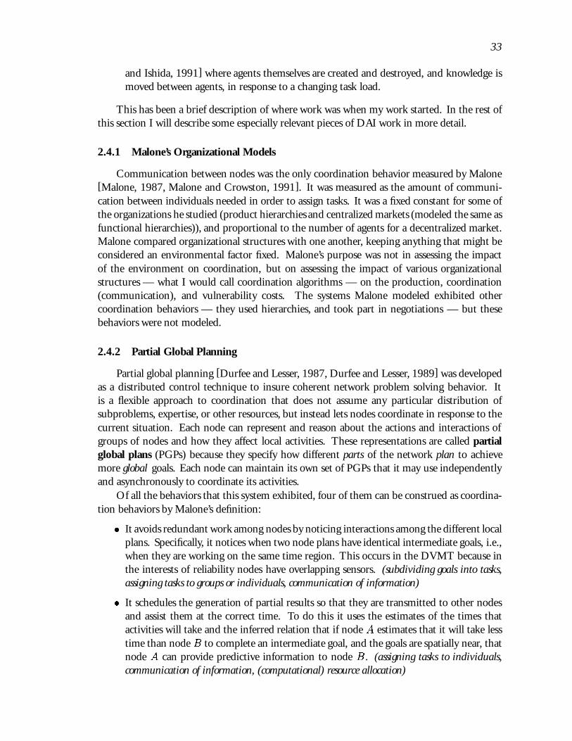
33

and Ishida, 1991] where agents themselves are created and destroyed, and knowledge ismoved between agents, in response to a changing task load.

This has been a brief description of where work was when my work started. In the rest ofthis section I will describe some especially relevant pieces of DAI work in more detail.

2.4.1 Malone’s Organizational Models

Communication between nodes was the only coordination behavior measured by Malone[Malone, 1987, Malone and Crowston, 1991]. It was measured as the amount of communi-cation between individuals needed in order to assign tasks. It was a fixed constant for some ofthe organizations he studied (product hierarchies and centralized markets (modeled the same asfunctional hierarchies)), and proportional to the number of agents for a decentralized market.Malone compared organizational structures with one another, keeping anything that might beconsidered an environmental factor fixed. Malone’s purpose was not in assessing the impactof the environment on coordination, but on assessing the impact of various organizationalstructures — what I would call coordination algorithms — on the production, coordination(communication), and vulnerability costs. The systems Malone modeled exhibited othercoordination behaviors — they used hierarchies, and took part in negotiations — but thesebehaviors were not modeled.

2.4.2 Partial Global Planning

Partial global planning [Durfee and Lesser, 1987, Durfee and Lesser, 1989] was developedas a distributed control technique to insure coherent network problem solving behavior. Itis a flexible approach to coordination that does not assume any particular distribution ofsubproblems, expertise, or other resources, but instead lets nodes coordinate in response to thecurrent situation. Each node can represent and reason about the actions and interactions ofgroups of nodes and how they affect local activities. These representations are called partialglobal plans (PGPs) because they specify how different parts of the network plan to achievemore global goals. Each node can maintain its own set of PGPs that it may use independentlyand asynchronously to coordinate its activities.

Of all the behaviors that this system exhibited, four of them can be construed as coordina-tion behaviors by Malone’s definition:

� It avoids redundant work among nodes by noticing interactions among the different localplans. Specifically, it notices when two node plans have identical intermediate goals, i.e.,when they are working on the same time region. This occurs in the DVMT because inthe interests of reliability nodes have overlapping sensors. (subdividing goals into tasks,assigning tasks to groups or individuals, communication of information)

� It schedules the generation of partial results so that they are transmitted to other nodesand assist them at the correct time. To do this it uses the estimates of the times thatactivities will take and the inferred relation that if node A estimates that it will take lesstime than node B to complete an intermediate goal, and the goals are spatially near, thatnode A can provide predictive information to node B. (assigning tasks to individuals,communication of information, (computational) resource allocation)

34

� It allocates excess tasks from overloaded nodes to idle nodes. Node plans provide theinformation needed to determine if a node is overburdened or underutilized. A nodeis underutilized if it is either idle or participates in only low-rated PGPs. A node isoverburdened if its estimated completion time of a subgoal of goal G is much later thanthe completion time of all the other subgoals of G [Durfee and Lesser, 1989]. (assigningtasks to groups or individuals, resource allocation)

� It assumes that a goal is more likely to be correct if it is compatible with goals at othernodes. In the DVMT task, a goal represented a processing task to ascertain whether avehicle was moving in a region r at time t. This goal could, in fact, be wrong — basedon noise or erroneous sensor data that was the basis for the preliminary task analysis thatgenerated the goal. Nodes choose local plans to work on based on the highly rated PGPsthey have received. Thus, if the intermediate goals of a node become part of a PGP, thenthey are worked on before other intermediate goals in other local plans the node mayhave (even though the node may have rated those local plans higher in its local view).(assigning tasks to groups or individuals, conflict resolution between agents)

In Durfee’s thesis [Durfee, 1987], the partial global planning mechanisms are claimed toexhibit most of the following coordination behaviors:

� Form subsolutions in parallel

� Form solution construction graphs (that show when partial results are to be deliveredand to whom)

� Exchange predictive information

� Assign important tasks to multiple agents

� Exchange tasks between agents

� Avoid redundant activities

� Verify other agent’s results

� Generate independent work

� Selectively exchange messages

As I will discuss in Section 5.1.1, the work on Generalized partial Global Planning (GPGP)that I will describe in Chapters 5 and 6 extends the PGP ideas. It does this by allowing moreagent heterogeneity, the exchange of more truly partially global information at multiple levelsof abstraction, the use of separate scheduling algorithms, etc. We will return to Partial GlobalPlanning in more detail when we introduce GPGP in Section 5.1.

2.4.3 Hierarchical Behavior Space

Early in this dissertation, I asserted that coordination behavior could be divided into threegeneral areas: specification (creating shared goals, instantiating goals into tasks and subdividingthem, standardization, etc.), planning, and scheduling. In more recent work, Durfee andMontgomery [Durfee and Montgomery, 1990] have worked on the specification side of things,developing a set of six hierarchies—who, what, when, where, how, and why—for specifyingagent behaviors. This rather arbitrary but nonetheless useful hierarchical standardization

35

mechanism allows goals to be specified, compared, and subdivided by potentially heterogeneousagents. Durfee and Montgomery also present a ‘protocol’ (algorithm) for using this informationfor scheduling coordination, however the mechanism is very general (agents communicate toavoid bad interactions and take advantage of positive interactions) and little work has beendone on prescribing exactly what is good behavior in a given environment (see the quote inSection 2.3.1). More recent work has shown that using abstraction does in fact result in lesscommunication [Montgomery and Durfee, 1992]. In the chapter on GPGP (Chapter 5) we willdiscuss several mechanisms that are much more detailed, and can be used together to constructan extendable family of coordination algorithms. One of those mechanisms (non-local view)tries to minimize communication; we have also argued elsewhere (and at about the same timeframe) that such a mechanism can be implemented in a hierarchical manner[Decker and Lesser,1992] to reduce communication.

2.4.4 Distributed AI and the Concept of Agency

The conception of agency in DAI has a different scope and direction from that of principal-agent theory (see Section 2.3.3). The primary theoretical focus has always been so called‘BDI’ (Beliefs, Desires, and Intentions) architectures, probably because of the long history ofmathematical logics of knowledge and belief extending back far before AI or modern computerscience (Halpern links it to the Greek study of epistemology (‘the study of knowledge’) [Halpern,1986]). A large amount of this work is not computational (e.g., Cohen and Levesque’s commentfrom the start of this chapter that they “: : : do not explore how these ideas [of intention and jointintention] can be applied in computational systems : : : ” [Levesque et al., 1990]). Informally,BDI architectures state exactly how an agent chooses its actions based on its current set ofbeliefs and its current set of desires (or goals). Intentions are used to link desires or goals (orplans to achieve goals) to actions.

A good example of a computational expression of these ideas is Shoham’s AGENT-0[Shoham, 1991]. It is not the only such expression (see for example at least [Halpern, 1986,Genesereth et al., 1986, Rosenschein and Genesereth, 1985, Cohen and Levesque, 1990,Zlotkin and Rosenschein, 1990, Gmytrasiewicz et al., 1991, Shoham, 1991, Jennings, 1993]),but it is a clear one. The construction of new agent architectures is not the subject of thisdissertation; this example is just one to use as a reference point when I talk about how agentsinteract with their environment later in the document. It is also useful to compare this withthe agent architecture used by the GPGP algorithm in Chapter 5.

Shoham’s AGENT-0 is really a simple interpreter based on the more general idea ofagent-oriented programming (AOP). AOP specializes the ideas of object-oriented programming(in the Actor sense) so that objects become agents that have a formally defined mental state (inthis case, beliefs, commitments, and capabilities rather than beliefs, desires, and intentions) andthat send messages to one another with types inspired by speech act theory (inform, request,offer, etc.). Commitments are a type of intention, and desires or goals come about from thespeech acts themselves (i.e., requests from other agents). AGENT-0 as a first pass explicitlyexcludes more complex intentional stances, plans, or goals and desires.

An agent program consists of some initialization and a set of unordered commitment rules.These commitment rules refer to the ‘current’ mental state of the agent (including currentincoming messages from other agents). The result of a commitment rule can be a commitment

36

to action at any future point in time. The underlying interpreter makes sure that the agentshonor their previous commitments.

The interpreter has only these two cycles: process the incoming messages (update localbeliefs and then update the commitments by running the commitment rules), and carryingout the commitments already made for the current time. Information from other agents ismarked as being the beliefs of these other agents (thus achieving common belief given perfectcommunication media); if it inconsistent with old beliefs then the old ones are removed(AGENT-0 allows only simple single facts and their negations, allowing this to happenfairly quickly). Rather than institute belief revision, AGENT-0 programs note importantpreconditions as part of the capability clause of a commitment (so retracting a belief can infact cause a commitment to be no longer carried out because the agent is no longer ‘capable’ ofdoing it). Such a retraction is always communicated to other agents.

2.4.5 Distributed AI and Distributed Processing

The problems and techniques of Distributed AI in purely computational systems aresomewhat related to those of the distributed computing community [Lampson et al., 1981,Paker and Verjus, 1983, v. Bochmann, 1983, Chambers et al., 1984, Stankovic, 1984a]. Thedifferences arise from several sources: focus, approach, and most importantly scope. Muchdistributed processing research is focused on the problems of data consistency and transactionprocessing that are not the focus of DAI research because DAI research avoids the creation ofconsistent global views. Thus one would never build a DAI system for handling bank transac-tions, but one might build a DAI application to search for instances of fraud on top of such asystem. Many distributed processing approaches to control and scheduling issues use centralizedsolutions—perfectly reasonable and efficient solutions in systems where the bottleneck is eithernot a problem or can be mitigated by special hardware. Many distributed scheduling approacheshave assumed that tasks are computationally independent; newer scheduling work admitsthe scheduling of task groups with precedence relationships (i.e., Spring [Zhao et al., 1987,Stankovic and Ramamritham, 1987]). Some techniques, such as contracting, have been used(independently) by researchers associated with both DAI and distributed computing systems[Malone et al., 1983, Malone et al., 1986]. Most of all, the scope of distributed processingwork is different; often it can provide a structure for the efficient implementation of DAIsystems. In Section 5.7 I will briefly discuss an interface between scheduling and decisionmaking applicable even to hard real-time scheduling; also see [Garvey and Lesser, 1994,Garvey et al., 1994].

2.4.5.1 Decentralized Control Theory

Classical and modern control theory is oriented mostly toward the control of continuousphysical processes. A single controller (agent) observes outputs from the environment (plant)and sets inputs that along with the current environment state determine the new outputs.Since control theory is the mathematical basis of most engineered systems, a large body of workexists. One introduction for computer scientists is Dean and Wellman [Dean and Wellman,1991]. Control theory has been used in AI control for continuous systems like robots. Thetypes of environments that we will model in this dissertation are in general not continuousbut discrete; less work has been done in discrete control theory. In this dissertation we are

37

interested in control in terms of choosing what activities to do and when to do them, whichis on the surface different from varying continuous plant input variables like the direction ofa robot’s travel or the temperature of a curing process. Of course the extremely general natureof control theory allows it to express even these types of problems, but few of the standardcontrol theoretic solution techniques are available. For example, the discrete task environmentswith complex interrelationships that we will model in this dissertation do not usually satisfythe superposition and homogeneity properties required for the system to be linear. Anotherdifference is that the models we will discuss in this dissertation are more highly structured thandynamical control theoretic models. Although it is far outside the scope of this dissertation, itwould be easier to develop automated tools for building TÆMS models than arbitrary dynamicalmodels of computer programs (as opposed to physical systems).

Extensions to control theory include stochastic control, where there is uncertainty in theenvironment’s response to inputs and uncertainty in the controller’s (agent’s) observations ofthe environmental outputs. The usual control theoretic approach to observational uncertaintyis the Kalman filter approach. This approach can be used to map from observations and a setof linear dynamical (control theoretic) models to a choice of one of these models that is the‘best’ (minimum mean-square error). It assumes evenly distributed Gaussian noise as it’s modelof uncertainty, which does not match all of the uncertainties in the systems we model—forexample, one would probably assume that the error in measuring durations of executablemethods would decrease over time.

Other extensions include decentralized control theory ([Siljak, 1991], for example), wherethere are multiple controllers (and plants). This situation is of course again somewhat closerto the multi-agent systems described in this dissertation, although still focussed on continuouslinear systems. A final important point to make about the applicability of control theory isthat some computer algorithms are currently being developed in the AI community (“anytimealgorithms” [Boddy and Dean, 1989]) and systems communities [Liu et al., 1991] that havecontinuous response characteristics, and thus some control theoretic techniques can be adaptedfor them.

2.4.5.2 Team Theory

Team theory [Ho, 1980] is a formalization of a simple distributed control decision problem.Stated informally, this problem is to find a decision rule for each of a set of agents that tells eachagent how to set each agent’s own ‘control’ given some set of potentially uncertain observations.Furthermore, the decision rules should minimize the expected value of a predetermined losscriteria based on what the agents do and the true state of nature.

The team theory formalization contains five components [Stankovic, 1984a]:

1. The state of nature: a vector of random variables with given distributions that representall the uncertainties that have some bearing on the problem

2. A set of observations on the state-of-nature vector for each agent, based on some functionof the true state-of-nature.

3. A set of decision variables or controls, one per decision maker

4. A decision rule (strategy) for each agent which chooses a value for an agent’s decisionvariable given the agent’s observation vector.

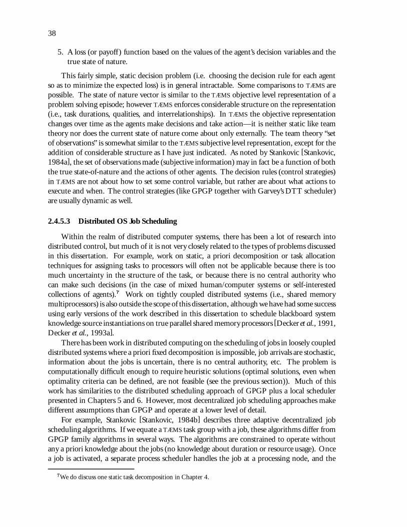
38

5. A loss (or payoff) function based on the values of the agent’s decision variables and thetrue state of nature.

This fairly simple, static decision problem (i.e. choosing the decision rule for each agentso as to minimize the expected loss) is in general intractable. Some comparisons to TÆMS arepossible. The state of nature vector is similar to the TÆMS objective level representation of aproblem solving episode; however TÆMS enforces considerable structure on the representation(i.e., task durations, qualities, and interrelationships). In TÆMS the objective representationchanges over time as the agents make decisions and take action—it is neither static like teamtheory nor does the current state of nature come about only externally. The team theory “setof observations” is somewhat similar to the TÆMS subjective level representation, except for theaddition of considerable structure as I have just indicated. As noted by Stankovic [Stankovic,1984a], the set of observations made (subjective information) may in fact be a function of boththe true state-of-nature and the actions of other agents. The decision rules (control strategies)in TÆMS are not about how to set some control variable, but rather are about what actions toexecute and when. The control strategies (like GPGP together with Garvey’s DTT scheduler)are usually dynamic as well.

2.4.5.3 Distributed OS Job Scheduling

Within the realm of distributed computer systems, there has been a lot of research intodistributed control, but much of it is not very closely related to the types of problems discussedin this dissertation. For example, work on static, a priori decomposition or task allocationtechniques for assigning tasks to processors will often not be applicable because there is toomuch uncertainty in the structure of the task, or because there is no central authority whocan make such decisions (in the case of mixed human/computer systems or self-interestedcollections of agents).7 Work on tightly coupled distributed systems (i.e., shared memorymultiprocessors) is also outside the scope of this dissertation, although we have had some successusing early versions of the work described in this dissertation to schedule blackboard systemknowledge source instantiations on true parallel shared memory processors [Decker et al., 1991,Decker et al., 1993a].

There has been work in distributed computing on the scheduling of jobs in loosely coupleddistributed systems where a priori fixed decomposition is impossible, job arrivals are stochastic,information about the jobs is uncertain, there is no central authority, etc. The problem iscomputationally difficult enough to require heuristic solutions (optimal solutions, even whenoptimality criteria can be defined, are not feasible (see the previous section)). Much of thiswork has similarities to the distributed scheduling approach of GPGP plus a local schedulerpresented in Chapters 5 and 6. However, most decentralized job scheduling approaches makedifferent assumptions than GPGP and operate at a lower level of detail.

For example, Stankovic [Stankovic, 1984b] describes three adaptive decentralized jobscheduling algorithms. If we equate a TÆMS task group with a job, these algorithms differ fromGPGP family algorithms in several ways. The algorithms are constrained to operate withoutany a priori knowledge about the jobs (no knowledge about duration or resource usage). Oncea job is activated, a separate process scheduler handles the job at a processing node, and the

7We do discuss one static task decomposition in Chapter 4.

39

job scheduler is no longer involved. The jobs are viewed by the scheduler as independent.Each of the algorithms is very simple an efficient, which is important since they are to beused at the operating system level. Similarly to GPGP-style algorithms, jobs may arrive atdifferent rates at different nodes, and the nodes communicate observations about how busythey are (observations that are out of date when they are received). Communication betweennodes takes non-negligible amounts of time. Stankovic [Stankovic, 1985] also has discusseddecentralized job scheduling using a Bayesian decision theoretic approach.

Work by Cheng, et al. [Cheng et al., 1986] on dynamic, heuristic real-time scheduling hasmore similarities. Like the GPGP+DTT approach, Cheng’s approach deals with groups of tasks(really executable methods in TÆMS terminology) that are interrelated. In Cheng’s case theseare precedence relationships only. All tasks in a group share a deadline. Tasks in a single groupcan be divided into clusters that can in turn be executed on different processors. Knowledge ofa task group is not available until the task group arrives at some node in the system. Differencesbetween this work and the GPGP+DTT approach include that all (or none) of the tasks in agroup must be scheduled, that tasks can execute at any node (homogeneity), and that biddingis used to decide where to transfer task group subclusters.

2.4.5.4 Game Theory

Game theory [Luce and Raiffa, 1958, Rasmusen, 1989] has been used to model decision-making situations faced by interacting agents and to show the existence of certain rationalstrategies for decision making. The model has been used in distributed AI to show howsystems of rational, self-interested agents can, in fact, “cooperate” without such cooperationbeing designed into them beforehand (the “benevolent agent assumption”) [Rosenschein andGenesereth, 1984, Rosenschein and Genesereth, 1985, Genesereth et al., 1986, Rosenscheinand Breese, 1989].

This early work represented a decision-making situation as a payoff matrix [Rapoport andGuyer, 1966] showing the utility to be gained by each agent for each possible choice of action.Such a simple representation allows strong results (including careful definitions of what theterm “rational” might mean with respect to computational agents [Rosenschein and Genesereth,1985]), but only under fairly restricted conditions. First, the payoff matrix represents only asingle decision. Secondly, most aspects of the problem, such as what choices are possible andthe utility of all of the outcomes, are known a priori by all the agents involved.

We can of course represent such simple situations in TÆMS. For example, Figure 2.1shows a representation of the traditional Prisoner’s Dilemma problem. Two agents suspectedof a crime are held in separate cells by the authorities. If both agents “cooperate” with oneanother (keep silent), the authorities can only charge them with a minor crime. If both “defect”(confess), the authorities charge them both. If one cooperates and the other defects, the defectoris set free and the other charged. We represent the agents’ individual utilities by /tems/ taskqualities. The initial qualities (q0) may change due to interactions between choices as shownin the figure. In general, given the restricted conditions above (that there is only one decisionto be made, and that all agents know everything about the decision at hand), it will always bepossible to create a payoff matrix from a TÆMS task structure.8 However, this dissertation will

8Thus some styles of deal-making and negotiation, represented in the game theory research, could be easilyadded to the GPGP set of coordination mechanisms.

40

focus on environments that consist of schedulable sequences of actions and uncertainty aboutthe local and non-local effects of those actions.

ADefects

q0=5

A

BDefects

q0=5

ACooperates

q0=3

BCooperates

q0=3

B

method executableby agent A only

method executableby agent B only

max task with qualityaccrual function max

subtask relationship

q=0

q=0

q=1

q=1

Figure 2.1. Secret agents A and B are captured and must decide whether to “Cooperate” withone another, or to “Defect”.

Work has been done on relaxing some of these constraints. For example, Axelrod [Axelrod,1984] talks about the effect of a continuous sequence of games on solutions to the Prisoner’sDilemma problem (i.e., the evolution of a “tit-for-tat” strategy). Kadane and Larkey [Kadaneand Larkey, 1982] discuss the addition of subjective probability. Rosenschein’s early and highlyinfluential work has led to more recent results in distributed AI. Rosenschein and Breese haveexperimented with probabilistic representations of other agents’ decisions [Rosenschein andBreese, 1989]. Gmytrasiewicz [Gmytrasiewicz et al., 1991, Durfee et al., 1993] has extendedthe model to recursively model the beliefs of other agents (the payoff matrix that A believes, thematrix that A believes that B believes, the matrix that A believes that B believes that A believes,etc.)

Still, the basic form of the model which represents a single decision can only easilyrepresent a certain class of problems. Rosenschein and his students have begun working inmore complex and general domains. Rosenschein and Zlotkin have coined three terms forthese increasingly complex domains: task oriented domains, state-oriented domains, and worthoriented domains. Task oriented domains are those where there is a bundle of non-conflicting

41

jobs to be done by a set of homogeneous agents (e.g. postal delivery) [Zlotkin and Rosenschein,1990, Zlotkin and Rosenschein, 1991]. State oriented domains have specific goals that theagents wish to achieve, and actions may interfere with one another (e.g. blocks world planning)[Ephrati and Rosenschein, 1994]. Worth oriented domains have some utility function forworld states, so that trade-offs are possible [Goldman and Rosenschein, 1993]. While wehave not yet worked on multi-agent planning and negotiation, TÆMS can obviously representworth-oriented environments and by inclusion the simpler types as well.

2.5 DAI Modeling

Up until very recently, there have been absolutely no analyses of distributed AI systemsthat have the generality of those in this dissertation, which were produced by our methodology.The sole exception is Sandip Sen’s work on distributed meeting scheduling [Sen and Durfee,1994]. This work was done at about the same time as my work. Sen analyzed the performance(success ratio in scheduling n meetings) and efficiency (cost of communication and totaltime to schedule) of several meeting scheduling heuristics. These heuristics included differentannouncement strategies, bidding strategies, and meeting confirmation strategies. Sen alsouses a probabilistic view of the environment, in this case the current schedules of two agentsfor a fixed time period, to compute formulas for the success ratio and total time. Sen verifiesthese using a simulation of two agents. Unlike our work, Sen actually runs the two agentsexhaustively on every possible starting condition (‘episode’, in our terminology).

2.6 Summary

The form of the TÆMS framework that I am about to describe in this dissertationis more detailed in structure than many organizational-theoretic models of organizationalenvironments, such as Thompson’s notions of pooled, sequential, and reciprocal processes[Thompson, 1967], Burton and Obel’s linear programs [Burton and Obel, 1984], or Malone’squeuing models [Malone, 1987], but is influenced by them, and by the importance ofenvironmental uncertainty, variance, and dependency that appear in contingency-theoreticand open systems views of organizations [Lawrence and Lorsch, 1967, Galbraith, 1977,Stinchcombe, 1990, Scott, 1987].

I started this chapter telling you that building task environment models would allow usto say much more precise things about systems, and might allow us to design coordinationalgorithms that are appropriate for the task environment at hand. I also told you that the formof that task environment model was inspired by social conceptions of task environments aswell as DAI research. The bulk of the chapter then discussed these social conceptions: first Idiscussed coordination behavior as conceived by four different schools of thought, and secondlyI discussed how the environment has an impact on coordination behavior, again from severalpoints of view. The chapter concluded with a discussion of the DAI view of coordinationbehaviors and several example systems.

In the next chapter I will introduce and describe in detail TÆMS, which is my modelingframework for representing and reasoning about task environments. The following chapterswill show TÆMS being used for mathematical analysis in a simplified distributed sensor network,and for simulation in an implementation of Generalized Partial Global Planning.

42

C H A P T E R 3

A FRAMEWORK FOR MODELING TASK ENVIRONMENTS

[and his students] : : : created a world of the mind, of the intimate imagination, whichis as real in its way as any actual country on the map. Sir Karl Popper, in one of hismost important papers, calls it ‘the third world,’ or ‘world three.’ The first world is theobjective world of things. The second world is my inner, subjective world. But, saysPopper, there’s a third world, the world of objective contents of thoughts. Teilhard deChardin calls this third world the noosphere, that is, the world of the mind.

— Sampled from an unknown source by The Orb, u.f.orb:“o.o.b.e”, 1992

This chapter will discuss the characterization of the features, and model of the processes,in computationally intensive task environments called TÆMS (Task Analysis, EnvironmentModeling, and Simulation) [Decker and Lesser, 1993d, Decker and Lesser, 1993e, Decker,1994c]. No characterization currently exists that formally captures the range of features,processes, and especially interrelationships that occur in computationally intensive AI taskenvironments. In the simplest terms, a TÆMS model of a task environment specifies what actionsare available to agents and how those actions relate to one another and to the performance ofthe system as a whole. The TÆMS framework is useful not only for the study of coordinationand other related CDPS behaviors (e.g., negotiation), but also for the study of the planningand scheduling of computation in realistic real-time or parallel task environments [Garvey etal., 1993, Garvey and Lesser, 1993].

The reason we have created the TÆMS framework is rooted in the desire to producegeneral theories in AI [Cohen, 1991]. Consider the difficulties facing an experimenter askingunder what environmental conditions a particular local scheduler produces acceptable results,or when the overhead associated with a certain coordination algorithm is acceptable giventhe frequency of particular subtask interrelationships. At the very least, our frameworkprovides a characterization of environmental features and a concrete, meaningful languagewith which to state correlations, causal explanations, and other forms of theories. The clearspecification of a computational task environment also allows the use of very strong analyticor experimental methodologies, including paired-response studies, ablation experiments, andparameter optimization. TÆMS exists as both a language for stating general hypotheses ortheories and as a system for simulation. The simulator is written in standard, object-orientedCommon Lisp (CLOS) for any platform. The simulator also supports the graphical displayof generated task structures, agent actions, and statistical data collection on the TI Explorerand DEC Alpha, via CLIM (Common Lisp Interface Manager) and CLIP (Common LispInstrumentation Package [Westbrook et al., 1994]).

This chapter will describe TÆMS in detail. First I will give a brief overview, then introducethe core modeling framework. Next, I will introduce the DSN (Distributed Sensor Network)

44

environment that I will use for the examples in the later chapters (and which I will analyze inChapter 4). Section 3.4 will then describe the language for building objective models of taskstructure instances in an environment. Section 3.5 will describe the way that TÆMS models thesubjective views that agents have about the objective task structure instances in the previouschapter. Finally, Section 3.6 will briefly describe the ways that TÆMS could model the processesof statistically generating objective and subjective task structures in an environment. Thatsection will also give examples of models outside of the DSN domain, such as hospital patientscheduling.

3.1 General Framework

The principle purpose of a TÆMS model is to analyze, explain, or predict the performance ofa system or some component. While TÆMS does not establish particular performance criteria,it focuses on providing two kinds of performance information: the temporal intervals of taskexecutions, and the quality of the execution or its result. Quality is an intentionally vaguely-defined term that must be instantiated for a particular environment and set of performancecriteria. Examples of quality measures include the precision, belief, or completeness of a taskresult. We will assume that quality is a single numeric term with an absolute scale, althoughthe algebra can be extended to vector terms. In a computationally intensive AI system, severalquantities—the quality produced by executing a task, the time taken to perform that task, thetime when a task can be started, its deadline, and whether the task is necessary at all—arearbitrarily affected by the execution of other tasks. In real-time problem solving, alternatetask execution methods may be available that trade-off time for quality. Agents do not haveunlimited access to the environment; what an agent believes and what is really there may bedifferent.

From the point of view of TÆMS an agent is a locus of belief and action. An agentmay “know” or “believe” in the existence of a certain task structure; the agent has a state. Acomputational agent might have a “belief database” where it stores information about the taskstructure.1 An agent may also execute methods that are part of this task structure it believes—this is called a “method execution action”. For example, Agent 1 might gain knowledge ofthe task structure in a certain problem solving episode. That task structure might contain anexecutable method M1. If Agent 1 executes this method, it will take some amount of time (asspecified in the model) and the agent will accrue some amount of quality (as specified in themodel). The action may have non-local effects on the actions (past, current, and future) ofother agents in the environment.

The model of environmental and task characteristics proposed has three levels: generative,objective, and subjective. The generative level describes the statistical characteristics required togenerate the objective and subjective episodes in an environment; it is a workload generator.A generative level model consists of a description of the generative processes or distributionsfrom which the range of alternative problem instances can be derived, and is used to study

1For the rest of this dissertation, we will usually refer to information the agent has as “belief ” and not“knowledge”, since agents will often have information in their databases that is false (but believed to be true).This is a very common epistemological distinction between knowledge and belief [Halpern and Moses, 1985,Halpern, 1986]. Since in almost any modal logic of knowledge and belief Knows(x)! Believes(x), we don’t loseany generality.

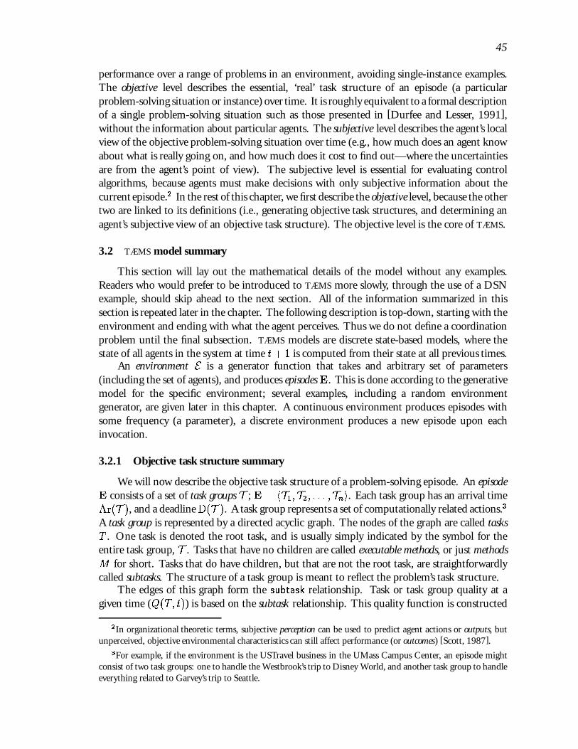
45

performance over a range of problems in an environment, avoiding single-instance examples.The objective level describes the essential, ‘real’ task structure of an episode (a particularproblem-solving situation or instance) over time. It is roughly equivalent to a formal descriptionof a single problem-solving situation such as those presented in [Durfee and Lesser, 1991],without the information about particular agents. The subjective level describes the agent’s localview of the objective problem-solving situation over time (e.g., how much does an agent knowabout what is really going on, and how much does it cost to find out—where the uncertaintiesare from the agent’s point of view). The subjective level is essential for evaluating controlalgorithms, because agents must make decisions with only subjective information about thecurrent episode.2 In the rest of this chapter, we first describe the objective level, because the othertwo are linked to its definitions (i.e., generating objective task structures, and determining anagent’s subjective view of an objective task structure). The objective level is the core of TÆMS.

3.2 TÆMS model summary

This section will lay out the mathematical details of the model without any examples.Readers who would prefer to be introduced to TÆMS more slowly, through the use of a DSNexample, should skip ahead to the next section. All of the information summarized in thissection is repeated later in the chapter. The following description is top-down, starting with theenvironment and ending with what the agent perceives. Thus we do not define a coordinationproblem until the final subsection. TÆMS models are discrete state-based models, where thestate of all agents in the system at time t+1 is computed from their state at all previous times.

An environment E is a generator function that takes and arbitrary set of parameters(including the set of agents), and produces episodes E. This is done according to the generativemodel for the specific environment; several examples, including a random environmentgenerator, are given later in this chapter. A continuous environment produces episodes withsome frequency (a parameter), a discrete environment produces a new episode upon eachinvocation.

3.2.1 Objective task structure summary

We will now describe the objective task structure of a problem-solving episode. An episodeE consists of a set of task groups T ; E = hT1;T2; : : : ;Tni. Each task group has an arrival timeAr(T ), and a deadline D(T ). A task group represents a set of computationally related actions.3

A task group is represented by a directed acyclic graph. The nodes of the graph are called tasksT . One task is denoted the root task, and is usually simply indicated by the symbol for theentire task group, T . Tasks that have no children are called executable methods, or just methodsM for short. Tasks that do have children, but that are not the root task, are straightforwardlycalled subtasks. The structure of a task group is meant to reflect the problem’s task structure.

The edges of this graph form the subtask relationship. Task or task group quality at agiven time (Q(T; t)) is based on the subtask relationship. This quality function is constructed

2In organizational theoretic terms, subjective perception can be used to predict agent actions or outputs, butunperceived, objective environmental characteristics can still affect performance (or outcomes) [Scott, 1987].

3For example, if the environment is the USTravel business in the UMass Campus Center, an episode mightconsist of two task groups: one to handle the Westbrook’s trip to Disney World, and another task group to handleeverything related to Garvey’s trip to Seattle.

46

recursively. Formally, the subtask relationship is defined as subtask(T;T; Q), where T is theset of all direct subtasks of T and Q is a quality function Q(T; t) : [tasks� times] 7! [quality]that returns the quality associated with T at time t. The semantics of a particular environmentare modeled by the appropriate choice of the quality function Q (e.g., minimum, maximum,summation, or the arithmetic mean). In particular, we will often write of the quality achievedat a task group at time t, Q(T ; t), meaning the current quality at the root task.

Executable methods represent domain actions, like executing a blackboard knowledgesource, running an instantiated plan, or executing a piece of code with its data.4 Executablemethods have several functions defined on them. q(M; t) is the current maximum quality thatcan be achieved by executing M at time t for its duration d(M; t). d(M; t) is the currentduration of method M at time t. Progress(M; t) is the number of time units spent executingM . The definitions of q(M; t), d(M; t), and Progress(M; t) are fixed by TÆMS. Q(M; t) isthe quality at M at time t. This function is available for modeling a particular environment,but it is constrained to obey the identity:

Q(M; t) = q(M; t) if [Progress(M; t) = d(M; t)] ^ [Finish(M) � D(M)]

(i.e. the quality is the maximum quality if the executable method was completed before itsdeadline).

Any task T containing a method that starts executing before the execution of anothermethod M finishes may potentially affect M ’s execution through a non-local effect e. We writethis relation (a labeled arc in the task structure graph) as nle(T;M; e; p1; p2; : : :), where thep’s are parameters specific to a class of effects. There are precisely two possible outcomes ofthe application of a non-local effect on M under our model: duration effects where d(M; t)(duration) is changed and quality effects where q(M; t) (maximum quality) is changed. Aneffect class e is thus a function e(T;M; t; d; q; p1; p2; : : :) : [task�method�time�duration�quality� parameter 1� parameter 2� : : :] 7! [duration� quality].

Computing d(M; t) and q(M; t). Each method has an initial maximum quality q0(M)and duration d0(M) so we define q(M; 0) = q0(M) and d(M; 0) = d0(M). If there is onlyone non-local effect withM as a consequentnle(T;M; e; p1; p2; : : :), then [d(M; t);q(M; t)] e(T;M; t;d(M; t � 1);q(M; t � 1); p1; p2; : : :). If there is more than one non-local effect,then the effects are applied one after the other in an order specified in the model. We willdefine sixteen example non-local effects in this chapter.

3.2.2 The subjective mapping and agent actions

We define a subjective mapping ' : [(x 2 E) �A� t] 7! x0 that maps from elements inthe current episode to agent A’s subjective view of those elements. The mapping may be emptyfor an element. This is the core of the subjective level model. Later in the chapter we discuss asimple default definition for '.5

Agents can perform three types of actions: they can execute methods, they can commu-nicate with one another, and they can perform “information gathering actions”. All of theseactions take some amount of time as specified in the model. For example, executing the method

4An executable method is always an action with context—thus “X-ray Nagi’s foot” is an executable method,while “X-ray” is not.

5One obvious extension is to make ' return a set of elements, not just one.

47

M at time t takes d(M; t), as we defined earlier. The main or “local” effect of this execution isthe production of some amount of quality at that node in the task structure (Q(M; t)). Thismay also change the quality at the task group root (Q(T ; t)). Executing a method may also havesecondary, or non-local effects, as defined earlier. A method might enable, hinder, facilitate,etc., other methods in the task structure by changing their current duration and maximumquality. Method execution actions are always part of the environment being modeled.

Communication actions and information gathering actions can be part of the environmentor can be meta-actions. Agents can communicate the results of any task. We define a specialquality function, Qavail(T;A; t) that returns the maximum of the quality available locally(Q(T; t)) and the quality that has been communicated to the agent. Communication takessome fixed amount of time between agents as specified in the model.6

Let �tA denote agent A’s set of beliefs at time t (the agent’s belief database). Externalinformation gets into the agent’s belief database via an information gathering action. Thedefault information gathering action places all communications that have arrived in the beliefdatabase, and places the subjective version ('(x;A; t)) of any newly-arrived elements of thecurrent episode in the belief database.

3.2.3 Coordination Problems

We can define a performance measure P(E) for the system (or for an agent) that isa function of the episode. The default is the sum of the task group qualities (P(E) =P

T 2EQ(T ;D(T ))). We can also define a control function (alternately, a “strategy”, decisionrule, or control policy) for each agent that given the agent’s current beliefs and the time willreturn the action that the agent should take at that time. One statement of a cooperativecoordinated control problem (similar in spirit to the specification of a team theory decisionproblem) is then to find a set of such control functions, one for each agent in an environment, soas to attempt to maximize the expected performance measure for the entire system of agents. Asimilar problem studied in DAI is the multi-agent self-interested coordination problem, wherewe choose an agent’s control function so as to attempt to maximize only it’s own performance(with the realization that other agents are doing likewise).

To summarize, using the TÆMS framework involves building a generative model of anenvironment that produces episodes that in turn comprise objective task structures. A subjectivemodel describes a mapping from these objective structures to the information available tothe agents (if the agents execute an information gathering action). All of this together is thedescription of the environment that can be used to design and analyze coordination mechanisms.The next section will introduce our in-depth example environment, a distributed sensor networkenvironment. Chapter 4 will analyze this environment and two control functions in detail.The rest of this chapter will focus first on the specification of objective task structures—themost complex and fully developed part of TÆMS. Then this chapter will discuss subjectiveand generative models, and give several short examples from many different problem solvingenvironments.

6Obvious extensions include extra complexity in the communication subnet model: lost messages, randomvariable delays, connectivity delays, etc.

48

3.3 Distributed Sensor Network Example

Before we discuss formally the basic components of an objective model, we turn to anexample environment for which we will build a model using the TÆMS framework. This examplegrows out of the set of single instance examples of distributed sensor network (DSN) problemspresented in [Durfee et al., 1987]. The authors of that paper compared the performanceof several different coordination algorithms on these examples, and concluded that no onealgorithm was always the best—not a very surprising result and one that can be viewed as thecentral tenet of contingency theory. This is the classic type of result that the TÆMS frameworkwas created to address—we will explain this result, and better yet, predict which algorithm willdo the best in each situation. In Chapter 4 we do this by extending the analysis to take intoaccount a statistical view of the environmental characteristics. The level of detail to whichyou build a model in TÆMS will depend on the question you wish to answer—here we wishto identify the characteristics of the DSN environment, or the organization of the agents, thatcause one algorithm to outperform another.

In a DSN problem (as you may recall from Chapter 1), the movements of severalindependent vehicles will be detected over a period of time by one or more distinct sensors,whereeach sensor is associated with an agent. The performance of agents in such an environmentis based on how long it takes them to create complete vehicle tracks, including the cost ofcommunication. The organizational structure of the agents will imply the portions of eachvehicle track that are sensed by each agent.

Our task environment model of naturally distributed problems assumes that severalindependent groups of tasks arrive at multiple locations over a period of time (the episode). Forexample, in a distributed sensor network (DSN) episode the movements of several independentvehicles will be detected over a period of time by one or more distinct sensors, where each sensoris associated with an agent. The performance of agents in such an environment will be basedon how long it takes them to process all the data into complete vehicle tracks, including thecost of communicating sensor data, intermediate task results, and meta-level communication,if any. The organizational structure of the agents will imply which subsets of which task groupsare available to which agents and at what cost. For example, if DSN agents have overlappingsensors, multiple agents can potentially work on data in the overlapping area (from its ownsensor) without any extra communication costs. We make several simplifying assumptions inthis DSN model: that the agents are homogeneous (have the same capabilities with respect toreceivingdata, communicating, and processing tasks), that the agents are cooperative (interestedin maximizing the system performance over maximizing their individual performance), thatthe data for each episode is available simultaneously to all agents as specified by their initialorganization, and that there are only structural (precedence) constraints within the subtasks ofeach task group.7

Any single episode can be specified by listing the task groups, and what part of eachtask group was available to which agents, given the organizational structure. Our analysesin Chapter 4 will be based on the statistical properties of episodes in an environment, notany single instance of an episode. The properties of the episodes in a DSN environment aresummarized by the tuple D =< A; �; r; o;T (l) > where A specifies the variable number of

7In general there are usually more complex interrelationships between subtasks that affect scheduling decisions,such as facilitation.

49

agents, � the expected number of task groups, r and o specify the variable structural portion ofthe organization by the range of each agent and the overlap between agents, and T (l) specifiesa template for the structure of each task group. Our DSN model will represent each vehicletrack as a separate task group, thus T (l) corresponds to a vehicle track of length l. DSN agentsensors are assumed to be square, and are arranged as a square. The range parameter specifiesthe physical range of the agent’s sensor (the width of a sensed square). The overlap parameterspecifies how wide the overlapping area sensed by two nearby agents is (0 � o � r). Figure 3.1shows an example. Later sections will describe in detail how the task group structures arespecified.

r=13

o=8

A=4

r=5

o=4

A=196

r=11

o=4

A=4

Figure 3.1. Examples of 18 � 18 DSN organizations

If the summary of a DSN environment is the tuple D =< A; �; r; o;T (l) >, then a par-ticular episode in this environment can be described by the tupleD =< T1(l1); : : : ;Tn(ln) >,where n is a random variable generated from a Poisson distribution with location parameter(central tendency) of �. The li are generated by a more complex process. For each track/taskgroup, two random points on two different sides of the bounding box around the agents’ sensorsare picked and a line is computed between them. Chapter 4 will analyze this distribution insome detail. We have just described how to generate an episode D in any DSN environmentD, by generating values for n and l1 : : : ln. This is the generative model.

In our objective-level model of DSN problem instances, each vehicle track is modeledas a task group Ti. Several task groups (vehicle tracks) may occur simultaneously in a singleproblem solving episode. The simplest objective model is that each task group Ti is associatedwith a track of length li and has the following objective structure, based on a simplified versionof the DVMT:

� (li) vehicle location methods (VLM) that represent processing raw signal data at a singlelocation resulting in a single vehicle location hypothesis

� (li � 1) vehicle tracking methods (VTM) that represent short tracks connecting theresults of the VLM at time t with the results of the VLM at time t+ 1

� One vehicle track completion method (VCM) that represents merging all the VTMstogether into a complete vehicle track hypothesis

Non-local effects, which relate the executions of tasks to one another, exist as shown inFigure 3.2—two VLMs enable each VTM, and all VTMs enable the lone VCM. This

50

structure is fairly common in many other environments, where a large amount of detailed workneeds to be done, the results of which are collected at a single location or agent and processedagain (integrated), and so on up a hierarchy. Coordination is used not only to accomplish thenecessary transfer of results from one agent to another, but to avoid redundant work on thepart of agents with overlapping capabilities, and also to potentially balance the workloads.

VTM

VCM

VLMVLM

VLMVLM

Tmin

VTM

VTM

TminT

min

Tmin

Tmin

method (executable task)

task with quality accrual function min

subtask relationship

enables relationship

Figure 3.2. Objective task structure associated with a single vehicle track.

We have used this model to develop expressions for the expected value and distributionof the time of termination of a set of agents in any arbitrary DSN environment that has astatic organizational structure and coordination algorithm (Chapter 4). We have also usedthis model to analyze a dynamic, one-shot reorganization algorithm (and have shown whenthe extra overhead is worthwhile versus the static algorithm. In each case we can predict theeffects of adding more agents, changing the relative cost of communication and computation,and changing how the agents are organized (in the range and overlap of their capabilities).These results were achieved by direct mathematical analysis of the model and verified throughsimulation in TÆMS. We will describe these results later (Chapter 4), after discussing moredetails about the the objective, subjective, and generative levels in this chapter.

3.4 TÆMS Objective Level Models

The objective level describes the essential structure of a particular problem-solving situationor instance over time. It focuses on how task interrelationships dynamically affect the qualityand duration of each task. The basic idea is that task groups (problem instances) appear inan episode at some frequency, and induce tasks T to be executed by the agents under study.

51

Task groups are computationally independent of one another, but tasks within a single taskgroup have interrelationships. Task groups and tasks may have deadlines D(T ). The quality ofthe execution or result of each task influences the quality of the task group result Q(T; t) in aformally-defined way (Section 3.4.1). These quantities can be used to evaluate the performanceof a system.

An individual task that has no subtasks is called a methodM and is the smallest schedulablechunk of work (though some scheduling algorithms will allow some methods to be preempted,and some schedulers will schedule at multiple levels of abstraction). There may be more thanone method to accomplish a task, and each method will take some amount of time and producea result of some quality. Quality of an agent’s performance on an individual task is a functionof the timing and choice of agent actions (‘local effects’), and possibly other (previous or future)task executions (‘non-local effects’). When local or non-local effects exist between tasks thatare known by more than one agent, we call them coordination relationships. The basic purposeof the objective model is to formally specify how the execution and timing of tasks affect themeasure of quality.

3.4.1 Local Effects: The Subtask Relationship

Task or task group quality (Q(T; t)) is based on the subtask relationship. This qualityfunction is constructed recursively—each task group consists of tasks, each of which consists ofsubtasks, etc.—until individual executable tasks (methods) are reached. Formally, the subtaskrelationship is defined as subtask(T;T; Q), whereT is the set of all direct subtasks of T andQ is a quality function Q(T; t) : [tasks� times] 7! [quality] that returns the quality associatedwith T at time t. In a valid model, the directed graph induced by this relationship is acyclic(no task has itself for a direct or indirect subtask). A task with no subtasks is called a method.Methods represent computation or physical actions; quality accrual at methods is described inthe next section.

The semantics of a particular environment are modeled by the appropriate choice of thequality function Q (e.g., minimum, maximum, summation, or the arithmetic mean). Forexample, if subtask(T1;T; Qmin), then Q(T1; t) = Qmin(T1; t) = minT2TQ(T; t). In thiscase the quality that is associated with task T1 is the minimum quality associated with any ofits subtasks. The four most popular non-method task quality combination functions are thefollowing:

Minimum. The quality that is generated is the minimum subtask value. This is sometimesreferred to as an AND (but see also Average below) because the quality of the parent remains ata minimum until every subtask has been completed. Often, this is used when all subtasks ofthe task must be completed before any value is generated (by making each method have quality0 before it is executed).

Qmin(T1; t) = minT2T

Q(T; t) (3.1)

Maximum. This is sometimes referred to as an XOR or OR (but see also Sum below)because only one subtask needs to be executed to gain quality at the parent task. Often this isused to model the situation where only one of the subtasks must be completed to receive value.One can construct situations where completing additional subtasks may generate additionalvalue. For example, if two tasks have potential maximum qualities of 10 and 5, and the agent

52

achieves the 5, the agent may at a later time come back and achieve the 10 (adding 5 to thequality of the parent).

Qmax(T1; t) = maxT2T

Q(T; t) (3.2)

Sum. This means that the quality generated for a task is the sum of the qualities generatedby its subtasks. Another common meaning for OR.

Q�(T1; t) =XT2T

Q(T; t) (3.3)

Average. This means that the quality generated for a task is the mean of the qualitygenerated by its subtasks. This is what the DVMT considered an AND.

Qavg(T1; t) =

PT2TQ(T; t)

jTj (3.4)

Other functions may be used for modeling particular environments.8 Another possiblefunction is one that represents diminishing returns to a fixed maximum, similar to the linearQlin function defined in the next section, or various convex curves such as 1

1�et. Functions like

sum and average indicate the possibility that not all tasks in the environment need to be carriedout. Computational task structures may represent search processes where agents are satisficing,not optimizing. We have now described how quality is modeled at tasks that have subtasks,and now turn our attention to methods.

3.4.2 Local Effects: Method Quality

Each method M at a time t will potentially produce (if executed by an agent, seeSection 3.5.3.1) some maximum quality q(M; t) after some amount of elapsed time d(M; t)(we will defer any further definition of the functions d and q until we discuss non-local effectsin Section 3.4.3). The execution of methods is interruptible, and if multiple methods for asingle task are available, the agent may switch between them (typically, alternative methodstradeoff time and quality). We model the effect of interruptions, if any, and the reuse of partialresults as non-local effects (see Section 3.4.3).

8The set of possible aggregation operators include three basic classes: conjunctions, disjunctions, and trade-offs.Dubois and Prade have shown that the Triangular norms (including min), averaging operators (including mean),and Triangular conorms (including max and summation) are the most general families of binary functions thatrespectively satisfy the semantic requirements of the three basic classes of aggregation operators [Bonissone andDecker, 1986, Dubois and Prade, 1984].

53

Let Progress(M; t) be the current amount of progress on the execution of M . If M werenot interruptible and Start(M) and Finish(M) were the execution start time and finish time,respectively, of M , then:

Progress(M; t) =

8><>:

0 t � Start(M)t � Start(M) Start(M) < t < Finish(M)Finish(M)� Start(M) t � Finish(M)

We typically model the quality produced by a method Q(M; t) using a linear growth functionQlin:

Qlin(M; t) =

(Progress(M;t)

d(M;t) (q(M; t)) Progress(M; t) < d(M; t)

q(M; t) Progress(M; t) � d(M; t)

Other models (besides linear quality functions) have been proposed and are used, such asconcave quality functions (must execute most of a task before quality begins to accumulate),convex quality functions (most quality is achieved early on in a method, and only small increasesoccur later), and ‘mandatory and optional parts’ quality functions [Liu et al., 1991]. The desiredQ(M; t) can be easily defined for any of these.

As an example of the power of this representation, we consider the two main schools ofthought on quality accumulation: the anytime algorithm camp [Boddy and Dean, 1989] andthe design-to-time (approximate processing) camp[Decker et al., 1990, Garvey and Lesser,1993]. We can represent their ideas succinctly; in the anytime algorithm model partial resultsare always available,9 as in the definition of Qlin(M; t) above, while in the design-to-timemodel results are not available (quality does not accrue) until the task is complete, as in thedefinition of QDTT(M; t):

QDTT(M; t) =

(0 Progress(M; t) < d(M; t)q(M; t) Progress(M; t) � d(M; t)

Another difference between design-to-time (DTT) and other approaches will show up in ourgenerative and subjective additions to this model—DTT does not assume that Q(M; t) is fixedand known, but rather that it is an estimator for the actual method response. Finally, deadlinescan be associated with task groups or individual tasks, and quality accumulation defined suchthat any work done on a task after its deadline does not increase quality.

3.4.3 Non-local Effects

Any task T containing a method that starts executing before the execution of anothermethod M finishes may potentially affect M ’s execution through a non-local effect e. We writethis relation nle(T;M; e; p1; p2; : : :), where the p’s are parameters specific to a class of effects.There are precisely two possible outcomes of the application of a non-local effect on M underour model:

duration effects: where d(M; t) (duration) is changed

quality effects: where q(M; t) (maximum quality) is changed.

9In Boddy’s paper, the assumption is made that Q(M; t) has monotonically decreasing gain.

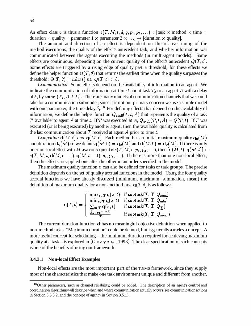
54

An effect class e is thus a function e(T;M; t; d; q; p1; p2; : : :) : [task � method � time �duration� quality� parameter 1� parameter 2� : : :] 7! [duration� quality].

The amount and direction of an effect is dependent on the relative timing of themethod executions, the quality of the effect’s antecedent task, and whether information wascommunicated between the agents executing the methods (in multi-agent models). Someeffects are continuous, depending on the current quality of the effect’s antecedent Q(T; t).Some effects are triggered by a rising edge of quality past a threshold; for these effects wedefine the helper function �(T; �) that returns the earliest time when the quality surpasses thethreshold: �(T; �) = min(t) s.t. Q(T; t) > �.

Communication. Some effects depend on the availability of information to an agent. Weindicate the communication of information at time t about task Ta to an agent A with a delayof �t by comm(Ta; A; t; �t). There are many models of communication channels that we couldtake for a communication submodel; since it is not our primary concern we use a simple modelwith one parameter, the time delay �t.10 For defining effects that depend on the availability ofinformation, we define the helper function Qavail(T; t;A) that represents the quality of a taskT ‘available’ to agent A at time t. If T was executed at A, Qavail(T; t;A) = Q(T; t). If T wasexecuted (or is being executed) by another agent, then the ‘available’ quality is calculated fromthe last communication about T received at agent A prior to time t.

Computing d(M; t) and q(M; t). Each method has an initial maximum quality q0(M)and duration d0(M) so we define q(M; 0) = q0(M) and d(M; 0) = d0(M). If there is onlyone non-local effect withM as a consequentnle(T;M; e; p1; p2; : : :), then [d(M; t);q(M; t)] e(T;M; t;d(M; t � 1);q(M; t � 1); p1; p2; : : :). If there is more than one non-local effect,then the effects are applied one after the other in an order specified in the model.

The maximum quality function q can also be defined for tasks or task groups. The precisedefinition depends on the set of quality accrual functions in the model. Using the four qualityaccrual functions we have already discussed (minimum, maximum, summation, mean) thedefinition of maximum quality for a non-method task q(T; t) is as follows:

q(T; t) =

8>>>><>>>>:

maxx2T q(x; t) if subtask(T;T; Qmax)minx2T q(x; t) if subtask(T;T; Qmin)P

x2T q(x; t) if subtask(T;T; Q�)Px2T

q(x;t)

jTjif subtask(T;T; Qmean)

The current duration function d has no meaningful objective definition when applied tonon-method tasks. “Maximum duration” could be defined, but is generally a useless concept. Amore useful concept for scheduling—the minimum duration required for achieving maximumquality at a task—is explored in [Garvey et al., 1993]. The clear specification of such conceptsis one of the benefits of using our framework.

3.4.3.1 Non-local Effect Examples

Non-local effects are the most important part of the TÆMS framework, since they supplymost of the characteristics that make one task environment unique and different from another.

10Other parameters, such as channel reliability, could be added. The description of an agent’s control andcoordination algorithms will describe when and where communicationactually occurs (see communicationactionsin Section 3.5.3.2, and the concept of agency in Section 3.5.1).

55

Typically a model will define different classes of effects, such as causes, facilitates, cancels,resource�constrains, inhibits, and enables [Decker and Lesser, 1992]. This section containsdefinitions for four common classes of effects that have been useful in modeling differentenvironments. When non-local effects occur between methods associated with different agents,we call them coordination relationships.

Enables. If task Ta enables method M , then the maximum quality q(M; t) = 0 until Tais completed and the result is available, when the maximum quality will change to the initialmaximum quality q(M; t) = q0(M). Another way to view this effect is that it changes the“earliest start time” of enabled method, because a rational scheduler will not execute the methodbefore it is enabled.

enables(Ta;M; t; d; q; �) =

([1; 0] t < �(Ta; �)[d0(M);q0(M)] t � �(Ta; �)

(3.5)

Facilitates. Another effect, used by the PGP algorithm [Durfee and Lesser, 1991] butnever formally defined, is the facilitates effect. In organization theory, Stinchcombe definesfacilitation as an ‘external effect’ in relation to the spatial properties of environmental activities[Stinchcombe, 1987], but also recognizes computational facilitation through the transmissionof information. Computationally, facilitation occurs when information from one task, often inthe form of constraints, is provided that either reduces or changes the search space to make someother task easier to solve. A simple to understand example of this relationship in computationis the relationship between sorting and searching. It is faster to retrieve an item from a sorteddata structure, but sorting is not necessary for retrieval. Hence the sorting task facilitates theretrieval task.

In our framework, one task may provide results to another task that facilitates the secondtask by decreasing the duration or increasing the quality of its partial result. Therefore thefacilitates effect has two constant parameters (called power parameters) 0 � �d � 1 and0 � �q � 1, that indicate the effect on duration and quality, respectively. The effect variesnot only through the power parameters, but also through the quality of the facilitating taskavailable when work on the facilitated task starts (the ratioR, defined below). Note that beforework is started on a method, Start(M) = t (i.e. formulae are evaluated as if execution wereabout to start).

R(Ta; s) =Qavail(Ta; s)

q(Ta; s)

facilitates(Ta;M; t; d; q; �d; �q) = [d(1� �dR(Ta; Start(M)));

q(1 + �qR(Ta; Start(M)))] (3.6)

So if Ta is completed with maximal quality, and the result is received before M is started, thenthe duration d(M; t) will be decreased by a percentage equal to the duration power �d of thefacilitates effect. The second clause of the definition indicates that communication after thestart of processing has no effect. In Chapter 6 we will explore the effects on coordination of afacilitates effect alone and with other effects.

Hinders. The hinders effect is the opposite of facilitates, because it increases the durationand decreases the maximum quality of the consequent. It can be used expressively in a model torepresent situations that reduce some baseline performance measures (as opposed to facilitates,which represents an increase in the baseline). Such situations occur computationally when

56

there are multiple methods for a task and one fails to provide as many constraints as the other.hinders can also be used as a high-level model of distraction [Durfee et al., 1987], whereinappropriate constraints communicated from one agent to another lead the second agent ona wild goose chase.

Precedence. We define the precedes effect as a combination of enables and hinders. Thatis, one task must be done before another and the first task must be done well or later taskswill suffer for it. This definition comes about because it models the behavior of the DVMT.If Ta precedes M , then M has infinite duration and 0 maximum quality until some qualityis accrued at Ta. Afterwards, the duration drops toward the initial value and the maximumquality increases to the initial value according to the ratio of available and maximum qualityand the precedence effect’s power parameters (�d � 0 and �q � 0). The following formula ismore easily understood if one keeps in mind that, in general, the ratio of available quality tomaximum quality will go from 0 to 1 as methods are executed.

precedes(Ta ;M; t; d; q; �d; �q) =

8<:

[1; 0] Qavail(Ta; Start(M )) � 0[d0(M )=R�d(Ta; Start(M ));q0(M )R�q(Ta; Start(M ))] Qavail(Ta; Start(M )) > 0

(3.7)

Causes. Task Ta causesmethod Mb, if the completion of the execution of Ta, in effect, alsocompletes the execution of Mb (potentially an action at a distance; no explicit communicationaction is implied) and all properties of the completion of Mb ensue. More formally:

causes(Ta;M; t; d; q; �) =

([d; q] t < �(Ta; �)[0; q] t � �(Ta; �)

(3.8)

Causal relationships are rare in the computational scheduling domains that most of our workhas been in.

Shares-Results. The general class of facilitates relationships can also be used to model theeffect of re-using partial results when switching between tasks (methods). This is modeledby the parameter 0 � � � 1, the retained time percentage. When � = 1, switching tasks islike starting over completely; when � = 0, the new method is credited with all the time usedunder the original method. For example, assume we have methods Ma and Mb, with durationsd(Ma) and d(Mb). Assume an agent starts using Ma and then switches to method Mb attime t1 < d(Ma) + Start(Ma). We defined sharing results (in [Garvey and Lesser, 1993]) asfollows:

shares�results(Ta;M; t; d; q; �) =([d; q] t < Start(M)[d� (1 � �)(Start(M)� Start(Ta)); q] t � Start(M)

Note that the final quality is always limited by the maximum quality of the last methodused (this definition could be expanded to hinder the following methods when going from alow-quality method to a higher-quality one; typically agents move from high- to low-quality,however). If there are several methods and the ‘better’ methods (with higher q(M)) shareresults with ‘worse’ methods, then credit for time spent is cumulative.

Cancels. Informally, Ta cancels Tb if the completion of Ta, without any communication,causes Q(Tb; t) = 0 for times t > Finish(Ta).

57

Favors. The favors relationship as described by von Martial [v. Martial, 1992] can beexpressed as a combination of relationships already described. To put it simply, it is not reallya new NLE (Non-Local Effect), but rather the presence of any positive (quality-improving)coordination relationship11.

Von Martial describes a favor action predicate that holds for actions (in TÆMS, we call themmethods): a favor action is an action which an agent does not have to execute locally and onethat “the agent would be pleased to have executed by another agent” [v. Martial, 1992]. VonMartial then defines a favor relationship between two plans as holding when there exists somefavor action a that is directly enabled by the plan actions, or can be enabled by adding a set ofactions to the plan. Of course not all possible favor actions are worthwhile or cost effective!We can represent von Martial’s concept in TÆMS as a relationship between a TÆMS method(the favor action) and a task (which represents a potential plan goal). A favors relationshipbetween a method M and a task T holds when the method M can positively effect T (directlyor indirectly) and M is executable by some agent beside the agent that has task T . That secondagent then has a possibility of doing a ‘favor’ for the first agent by scheduling and executingM . How much of a ‘favor’ it is depends on the local utility of executing M , from the point ofview of the agent offering the favor. M might be in that agent’s current schedule, so the favoris essentially for free (except for communication and any necessary temporal synchronization,including a deadline on the completion of M ). Alternately, M might not be in the currentschedule, and a new schedule and a potentially new set of actions would be needed before andafter executing M . Our definition is broader than von Martial’s because the favor action M inour case does not have to be executable by both agents (only the agent who is doing the favor).

Figure 3.3 shows the canonical von Martial post office example. Assume that there aretwo agents and that each agent has a method for every task in the picture. Also assume thatagent 1 wants to buy some stamps (task T1) and agent 2 wants to mail a package (task T2).The fact that agent 1 can execute a method for ‘mail package’, and the presence of the subtaskrelationship between ‘mail package’12 and task T2 means that agent 1 can do a ‘favor’ for agent2 and do the ‘mail package’ task. Since agent 1 is already buying stamps, and thus alreadygoing to the post office and returning, such a favor might be fairly inexpensive. However,notice that packages must be mailed at the post office counter, while stamps can be bought ata self-service machine. If agent 1 is on a very tight schedule, it might not be possible to use thelonger duration ‘use counter’ method. On the other hand, the same favor relationship existsfrom ‘buy stamps’ to task T1—agent 2 can also do a favor for agent 1 and buy the stamps.Since agent 2 is already committed to using the counter, no extra wait is involved.

Although I will not talk about the GPGP coordination mechanisms until Chapter 5, Iwill briefly discuss the implementation of a von Martial ‘favors’ coordination mechanism forcooperative agents. Such a mechanism would communicate the names of tasks on which agentswant to achieve quality. Let’s call these named tasks ‘goals’. Agents then loop through eachfavor action (in von Martial’s case, any action that can be executed by more than one agent;in our case the more general definition of any method or task that is related by a positivecoordination relationship to another agent). If the favor action can positively affect the other

11Remember, a coordination relationship is an NLE between task structures at different agents.12‘Mail package’ is the favor action in the definition in the last paragraph, and subtask is the coordination

relationship.

58

Go to PostOffice

Buystamps(max)

Mailpackage

Returnfrom Post

Office

Usemachine

UseCounter(shorter

duration)(longerduration)

max task with qualityaccrual function max

subtask relationship

enables relationship

T1 T2

Figure 3.3. Objective task structure associated with visiting the post office to buy stamps and/ormail a package. Assume that every agent has a local method for each of these tasks.

agent’s goals, then we mark it as a potential favor for that agent. This part of the algorithmis a straightforward restatement of von Martial’s algorithm. At this point, von Martial wouldcompute certain cost measures; in our case, we would query the local scheduler for the effectof adding a Do commitment on the favor action.

3.4.3.2 An Example of Facilitates and Shares-results

In this example we have one task group with two tasks, Ta and Tb, each with twomethods, M1 and M2, and the non-local relationships indicated in Figure 3.4. For both tasks,q(M1) = 20 and q(M2) = 5, and d(M1) = 15 and d(M2) = 5. This example depends onour view of method execution at an agent that is discussed in Section 3.5.3.1.

This example uses the following assumptions:

� the execution of M1A begins at time 0

� at time 4 the agent switches from method M1A to M2A

� communication of results from task Ta to task Tb occurs at the completion of M2A (withno time delay)

� we use the linear quality model Qlin

� method M2b is scheduled for task Tb

Quality associated with each task and method then accrues over time as shown in Figure 3.5.

59

T∑

AMax

M1A M2A M1B M2B

BMax

facilitates(50%)

shares-result(50 %)shares-result(50 %)

Figure 3.4. A simple model of two tasks with two methods each.

3.4.4 Expanding the DSN Model

We will now add some complexity to the distributed sensor network model. The lengthof a track li mentioned earlier is a generative model parameter. Given a set of these generativeparameters, we can construct the objective model for a specific episode (problem-solvinginstance). Figure 3.2 shows the general structure of episodes in our DSN environment model.To display an actual objective model, let us assume a simple, concrete situation: there aretwo agents, A and B, and that there is one vehicle track of length 3 sensed once by Aalone (T 1), once by both A and B (T 2), and once by B alone (T 3). We now proceedto model the standard features that have appeared in our DVMT work for the past severalyears. We will add the characteristic that each agent has two methods with which to dealwith sensed data: a normal VLM and a ‘level-hopping’ (LH) VLM (the level-hopping VLMproduces less quality than the full method but requires less time; see [Decker et al., 1990,Decker et al., 1993b] for this and other approximate methods; a similar technique can be usedto model agents who have different capabilities such as processor speed). Furthermore, only theagent that senses the data can execute the associated VLM; but any agent can execute VTMsand VCMs if the appropriate enablement conditions are met.

Figure 3.6 displays this particular problem-solving episode. To the description above, wehave added the fact that agent B has a faulty sensor (the durations of the grayed methodswill be longer than normal); we will explore the implications of this after we have discussedthe subjective level of the framework in the next section. An assumption made in [Durfeeet al., 1987] is that redundant work is not generally useful; this is indicated by using max asthe combination function for each agent’s redundant methods. This would not be a goodassumption for an environment where the independent derivation of a result is a positivething—we can alter the assumption by simply changing this function (to mean or sum).Another characteristic that appeared often in the DVMT literature is the sharing of resultsbetween methods (at a single agent); we would indicate this by the presence of a sharingrelationship (similar to facilitates) between each pair of normal and level-hopping VLMs

60

0

2

4

0 5 10 15 20

0

3

5

0 5 10 15 20

0

3

5

0 5 10 15 20

0 5 10 15 20

0

3

6

0 5 10 15 20

0

3

6

0 5 10 15 20

Time

0.0

6.0

12.0

0 5 10 15 20

Q(M

1A)

Q(M

2A)

Q(A

)Q

(M1B

)Q

(M2B

)Q

(B)

Q(T

)

Figure 3.5. Quality at each Method, Task, and Task Group over time in the previous figure

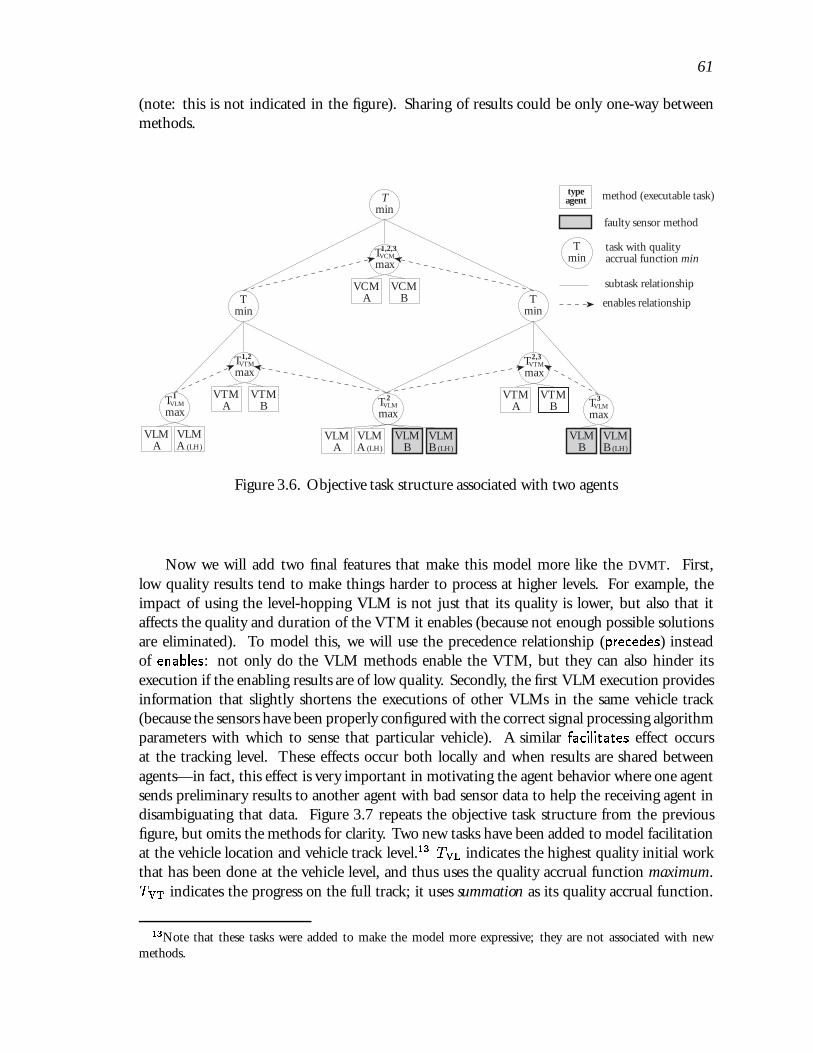
61

(note: this is not indicated in the figure). Sharing of results could be only one-way betweenmethods.

faulty sensor method

Tmin

task with quality accrual function min

subtask relationship

enables relationship

method (executable task)

VCMA T

minT

min

Tmin

VCMB

VTMA

VTMB

VTMA

VTMB

VLMA (LH)

VLMB

VLMA

VLMB (LH)

VLMA (LH)

TVLM

max

VLMA

VLMB

VLMB (LH)

TVLM

maxTVLM

max

TVTM

maxTVTM

max

TVCM

max

1

2,31,2

2 3

1,2,3

typeagent

Figure 3.6. Objective task structure associated with two agents

Now we will add two final features that make this model more like the DVMT. First,low quality results tend to make things harder to process at higher levels. For example, theimpact of using the level-hopping VLM is not just that its quality is lower, but also that itaffects the quality and duration of the VTM it enables (because not enough possible solutionsare eliminated). To model this, we will use the precedence relationship (precedes) insteadof enables: not only do the VLM methods enable the VTM, but they can also hinder itsexecution if the enabling results are of low quality. Secondly, the first VLM execution providesinformation that slightly shortens the executions of other VLMs in the same vehicle track(because the sensors have been properly configured with the correct signal processing algorithmparameters with which to sense that particular vehicle). A similar facilitates effect occursat the tracking level. These effects occur both locally and when results are shared betweenagents—in fact, this effect is very important in motivating the agent behavior where one agentsends preliminary results to another agent with bad sensor data to help the receiving agent indisambiguating that data. Figure 3.7 repeats the objective task structure from the previousfigure, but omits the methods for clarity. Two new tasks have been added to model facilitationat the vehicle location and vehicle track level.13 TVL indicates the highest quality initial workthat has been done at the vehicle level, and thus uses the quality accrual function maximum.TVT indicates the progress on the full track; it uses summation as its quality accrual function.

13Note that these tasks were added to make the model more expressive; they are not associated with newmethods.

62

The more tracking methods are executed, the easier the remaining ones become.14 This modelhas implications for a multi-agent episode. For instance, the model describes the effect of thecommunication time on communicating partial results to another agent: the later an agentdelays communication, the more the potential impact on the other agent (because the qualityis increasing), but the more the other agent must delay. We examine this question in somewhatmore detail in Chapters 4, 5, and 6.

Tmin

task with quality accrual function min

subtask relationship

precedence relationship

facilitates relationship

Tmin

Tmin

Tmin

TVLM

maxTVLM

maxTVLM

max

TVTM

maxTVTM

max

TVCM

max

TVL

max

TVT

Σ

1

2,31,2

2 3

1,2,3

Figure 3.7. Non-local effects in the objective task structure

At the end of the next section, we will return to this example and add to it subjectivefeatures: what information is available to agents, when, and at what cost.

3.4.5 Resources

Physical resources, be they people, equipment, or computational resources such as files, arevery important to model in many domains [Zhao et al., 1987, Cheng et al., 1988, Ramamrithamet al., 1990, Shen et al., 1993, Sycara et al., 1991, Neiman et al., 1994]. This dissertation ismainly concerned with the modeling of computational task structures that do not use externalphysical resources (physical resources other than the processor). This section will brieflydescribe how we could extend TÆMS to model physical resources. The rest of the dissertationwill concentrate on purely computational environments—we will not carry out any simulationexperiments with physical resources in this dissertation. We believe this is an important futuredirection, see the Future Work section in Chapter 7.

14In the real DVMT, the effect only works to a point, so that the first four data points or so bring about mostof the effect. We could model this more precisely by replacing the summation with a Max and a Sum (a piecewiselinear approximation) or by using an exponential ( 1

1�ex).

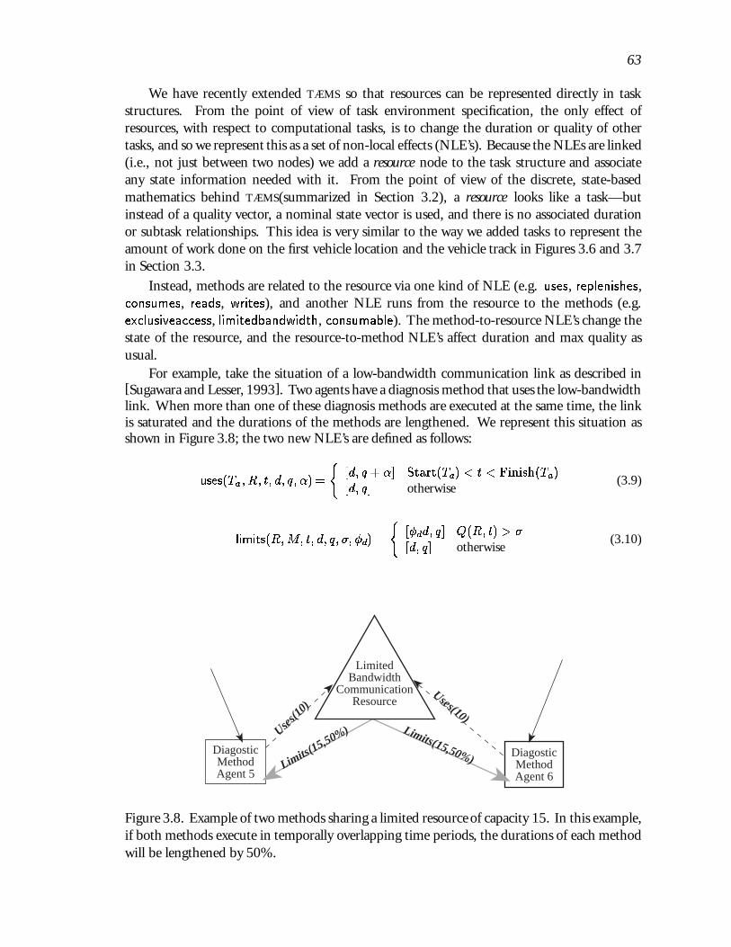
63

We have recently extended TÆMS so that resources can be represented directly in taskstructures. From the point of view of task environment specification, the only effect ofresources, with respect to computational tasks, is to change the duration or quality of othertasks, and so we represent this as a set of non-local effects (NLE’s). Because the NLEs are linked(i.e., not just between two nodes) we add a resource node to the task structure and associateany state information needed with it. From the point of view of the discrete, state-basedmathematics behind TÆMS(summarized in Section 3.2), a resource looks like a task—butinstead of a quality vector, a nominal state vector is used, and there is no associated durationor subtask relationships. This idea is very similar to the way we added tasks to represent theamount of work done on the first vehicle location and the vehicle track in Figures 3.6 and 3.7in Section 3.3.

Instead, methods are related to the resource via one kind of NLE (e.g. uses, replenishes,consumes, reads, writes), and another NLE runs from the resource to the methods (e.g.exclusiveaccess, limitedbandwidth, consumable). The method-to-resource NLE’s change thestate of the resource, and the resource-to-method NLE’s affect duration and max quality asusual.

For example, take the situation of a low-bandwidth communication link as described in[Sugawara and Lesser, 1993]. Two agents have a diagnosis method that uses the low-bandwidthlink. When more than one of these diagnosis methods are executed at the same time, the linkis saturated and the durations of the methods are lengthened. We represent this situation asshown in Figure 3.8; the two new NLE’s are defined as follows:

uses(Ta; R; t; d; q; �) =

([d; q + �] Start(Ta) < t < Finish(Ta)[d; q] otherwise

(3.9)

limits(R;M; t; d; q; �; �d) =

([�dd; q] Q(R; t) > �

[d; q] otherwise(3.10)

DiagosticMethodAgent 5

DiagosticMethodAgent 6

LimitedBandwidth

CommunicationResource

Uses(1

0)Uses(10)

Limits(15,50%)Limits(15,50%)

Figure 3.8. Example of two methods sharing a limited resource of capacity 15. In this example,if both methods execute in temporally overlapping time periods, the durations of each methodwill be lengthened by 50%.

64

The NLE uses indicates the amount of limited resource capacity used by the method withthe parameter �. In Figure 3.8 each diagnostic method uses 10 units of the communicationresource’s capacity (the arc labeled uses(10)). The NLE limits indicates that the resource hasmaximum capacity (saturation) � and that beyond that point duration is affected by percentage�d (alternately, �d could be defined as a function of the level of oversaturation). In Figure 3.8the communication resourcehas a saturation point � = 15, so the resource will not be saturatedif either diagnostic method uses the resource alone, and will be saturated if the two methodshappen to overlap in their execution. The effect will only be active during the overlap, and willcause the duration of both methods to be increased (in this example) by 50%. Note that whenmethods can be interrupted, the lengthening of method durations due to a blocked resource isnot associated with lengthening the amount of continuous computation—the blocked methodcan be interrupted and other computations performed until the method is no longer blocked.

It is important to note that our purpose here is not to develop a full-fledged resourcerepresentation language, but merely to argue that we could do so at a later time (see FutureWork in Chapter 7). The extensibility of TÆMS, including the addition of new task andresource relationships, is one of its major advantages. The exciting thing is that at the lowestlevel, we can define resource effects without adding to the basic, simple TÆMS mechanisms.Note that the formulae above and below use the Quality variable to hold state information forthe resource; if a resource requires more than one state variable then we can represent it byusing a quality vector, as we noted at the start of this chapter.

M1

M2

M3R1Con

sumes(10) Consumes(10)

Consumable(10) Consumable(10)

Reple

nish

es(1

0) Full(100)

Figure 3.9. Example objective structure of two methods (M1 and M3) that consume a resource,and one method that replenishes it.

Similar NLE’s can be defined for representing consumable resources and their associatedoperations (see Figure 3.9):

consumes(Ta; R; t; d; q; �) =

([d; q� �] t > Finish(Ta)[d; q] otherwise

(3.11)

consumable(R;M; t; d; q; �) =

([1; 0] Q(R; t) < �

[d; q] otherwise(3.12)

65

replenishes(Ta; R; t; d; q; �) =

([d; q+ �] t > Finish(Ta)[d; q] otherwise

(3.13)

full(R;M; t; d; q; �) =

([1; 0] Q(R; t) > �

[d; q] otherwise(3.14)

Thus in Figure 3.9 Methods 1 and 2 consume 10 units of Resource 1, if that amount is availableand Method 3 when executed replenishes Resource 1 by 10 units, unless Resource 1 already hasover 100 units, in which case it cannot be replenished (it is ‘full’). Note that this is an objectiveexample. A generative model would (for example) say if Method 1 always consumes 10 unitsor Resource 1, or if the amount is drawn from some distribution. The subjective model wouldsay if an agent, making a decision about Method 1, “knows” that Method 1, in fact, consumes10 units, or believes that it consumes more or less units, or knows only the generative model.

3.5 TÆMS Subjective Level Models and Agent Actions

The purpose of a subjective level model of an environment is to describe what portions ofthe objective model of the situation (current state) are available to ‘agents’. It answers questionssuch as “when is a piece of information available,” “to whom is it available,” and “what is the costto the agent of that piece of information”. This is a description of how agents might interactwith their environment—what options are available to them. Of course agents both acquireinformation and act on that information. This chapter will discuss agent actions—acquiringinformation, executing methods, and communicating with one another.

To build such a description we must introduce the concept of agency into the model. Oursis one of the few comprehensive descriptions of computational task environments in AI, butthere are many formal and informal descriptions of the concept of agency (see [Gasser, 1991,Hewitt, 1991, Moe, 1984], Sections 2.3.3 and 2.4.4). Rather than add our own description,we notice that these formulations define the notion of computation at one or more agents, notthe environment that the agents are part of. Most formulations contain a notion of belief thatcan be applied to our concept of “what information an agent has about its environment”. Ourview is that an “agent” is a locus of belief and action (such as computation), as stated in theintroduction to this chapter.

The form of the rest of this section is as follows:

� How does the environment affect the beliefs of the agents? This is described by a TÆMS

“subjective” level model.

� How do the beliefs of agents affect their actions? This is basis of the coordinationand control problem. The rest of the dissertation will describe and analyze variousmechanisms to accomplish this step.

� How do the actions of the agents affect the environment? /tems/ is a discrete, state-basedmodel. We will describe in this section how the state of the environment and the agentschanges when the agents act. There are three types of agent actions: method executions,communications, and information gathering actions.

66

3.5.1 The Subjective Mapping

Each agent can be thought of to have a “belief database” �A. We use the symbol �tA todenote this set of beliefs of agent A at time t. We will use the modal operator Bt

A(x) to meanagent A subjectively believes x at time t, that is, �tA j= x (from Shoham[Shoham, 1991]).

We define a subjective mapping ' : [(x 2 E) �A� t] 7! x0 that maps from elements inthe current episode to agent A’s subjective view of those elements. The mapping may be emptyfor an element. This is the core of the subjective level model. For example, we could definea mapping ' where each agent has a probability p of believing that the maximum quality ofa method is the objective value, and a probability 1 � p of believing the maximum qualityis twice the objective value. Any objective assertion has some subjective mapping, includingq (maximum quality of a method), d (duration of a method), deadlines, and the relationssubtask, nle, and comm and their associated parameters. Section 3.5.4 will describe a fewexamples of this mapping.

Finally, we will define an action that can be taken by an agent, called an informationgathering action, which will take some amount of time and result in the addition of newinformation to the agent’s belief database. In particular, we define a task arrival informationgathering action such that

�A ; �A [ '(x;A; t)j(x 2 E) ^ ('(x;A; t) 62 �A)

This action places a subjective version of new information from the objective episode into theagent’s belief database.

3.5.2 Deciding What to Do Next: Coordination, Scheduling, and Control

The beliefs of an agent affect its actions through some control mechanism. Since this is thefocus of most of our and others’ research on local scheduling, coordination, and other controlissues, we will not discuss this further in this chapter (but see Chapters 4 through 6). The agent’scontrol mechanism uses the agent’s current set of beliefs �A to update three special subsets ofthese beliefs I; C;M� �A defined here as the sets of information gathering, communication,and method execution actions to be computed. These subsets describe the agent’s intentions.For example, if an agent intends to execute method M1, it creates a method execution actionthat indicates M1 as the method to execute.15 The agent then adds this method executionaction set of intended method executionsM. The next section describes what happens to anagent’s intended actions.

The agents that we build typically further divide control into local scheduling and co-ordination (see Chapters 5 and 6), but this is not required. Besides describing how anagent’s beliefs entail commitments to particular information gathering, communication, andmethod execution actions, a control component model must also describe the duration of itsdeliberations. This feature allows us to analyze questions concerning the cost of control withoutbecoming mired in implementation details.16

15It might indicate other things, like on which processor to execute M1 if the agent is a multiprocessor, or atime limit for M1, execution monitoring information, etc. None of these extensions are a part of this dissertation.

16Understanding the details of the control costs of particular algorithm implementations is important, butusually not at early stages of research. Information about control duration can also be used by the TÆMS simulatorif it is available.

67

3.5.3 Computation

Our model can support parallel computation, but for brevity we will just describe singleprocessor computation as a sequence of agent states. Agent A’s current state is uniquelyspecified by �A. We provide a meta-structure for the agent’s state-transition function that isdivided into the following 4 parts (see also Figure 3.10:

1. control (as described in the previous section—basically asserting one or more intentions)

2. method execution (of the methods inM)

3. information gathering (doing the information gathering actions in I)

4. communication (doing the communication actions in C)

start

Control InformationGathering

Communication

MethodExecution

I≠Ø

I≠Ø

C=Ø

I=Ø I=Ø

C=Ø C≠Ø

C≠Ø

M=Ø

M=Ø

M≠Ø

M≠Ø

Figure 3.10. The finite state machine that describes the meta-structure of single-processor agentcomputations. I; C;M are named subsets of the agents beliefs � that represent informationgathering, communication, and method execution actions, respectively.

First the control mechanisms assert (“intend”) information-gathering, communication,and method execution actions and then these actions are computed one at a time, after whichthe cycle of meta-states repeats.

A simple model of parallel computation, similar to the implementation in [Decker et al.,1993a], is to allow control, information gathering, and communication to run on one (abstract)processor, and multiple method executions on the other processors. Any important interactionsbetween methods executing in parallel would be represented by non-local effects.

68

3.5.3.1 Method Execution

How do the actions of an agent affect the environment? Both the objective environment(e.g. quality of the executing method) and the subjective mapping (e.g. information availablevia ') can be affected. We use two execution models: simple method execution, and executionwith monitoring, suspension, and preemption. These follow from the discussion of QDTT andQlin in Section 3.4.2, and are simple state-based models. Basically, for non-interruptible, singleprocessor method executions, the agent enters a method execution state for method M at timeStart(M) and remains in that state until the time t when t� Start(M) = d(M; t). Methodexecution actions are similar to what Shoham terms ‘private actions’ like DO[Shoham, 1991].

We have also considered pre-emptable method execution, where a method execution actionis given a set upper time limit, after which computation will proceed to the next meta-state.The agent can then monitor the execution of long methods, and interleave their execution withother actions or pre-empt them entirely [Garvey and Lesser, 1993].

Formal Definition of Simple Method Execution. Let M 2 M be the method that anagent is about to execute. We identify several parts of the objective model O of the externalenvironment: q(M; t), the true maximum quality of M at time t computed from some initialq0(M) and all of the non-local effects on M as described in Section 3.4.3; d(M; t), the trueduration of M at time t computed from some initial d0(M) and all of the non-local effects onM as described in Section 3.4.3; and Q, the mathematical model of the way quality accruesduring the execution of M (QDTT, for example).

At the start of execution at time t0, the state of the environment is updated by an agentA such that hStart(M) = t0i 2 O. The state of the environment includes the values ofq(M; t0) and d(M; t0) computed as described in Section 3.4.3. Agent A at time t0 is in a statewhere it believes Bt0

A hStart(M) = t0;q(M; t0) = '(q(M; t0));d(M; t0) = '(d(M; t0))i.Depending on the model of quality accrual Q, the quality of M at time t + 1 may change,which may trigger non-local effects, etc.

From its state at an arbitrary time t the environment moves to a new state at timet + 1 by updating the values of q and d for all M , given the addition of new start timesStart(M) for methods as agents execute them, and new finish times Finish(M) as agentsfinish execution (described next). The agent also moves to a new state at time t + 1: ift+1 < Start(M)+d(M; t)17 then the agent remains in the state where it believesBt+1

A = BtA,

otherwise it finishes execution, and adds to its beliefs and the objective model the assertionFinish(M) = t+ 1.

The simple model of execution does not allow agents to preempt, suspend, or otherwisemodify the execution of a single method. This capability can be added by extending thismodel so that a method execution intention is a pair [M; t] = M which means to executeM for t time units, or until it finishes, if it finishes early. This simple extension allows bothmonitoring and preemption, and improves the model because the local scheduler can intendinformation-gathering actions (i.e., see if new tasks have arrived) at the monitoring points.

3.5.3.2 Communication

How do the actions of an agent affect other agents? Communication actions allow agentsto affect each others’ beliefs to a limited extent. Many people have worked on formalizing

17Note that d(M; t) is the actual objective duration of M at time t, not the agent’s belief in its duration.

69

aspects of communication; the semantics of communication actions can be freely defined foreach environment. The simplest communication act is to send another agent the ‘currentresult/value’ of a method—the effect is to change the available quality Qavail(T; t;A) at theremote agent after the message has been received. What happens when a communication is‘received’? The reception of information, by changing the available quality of a task, maytrigger a non-local effect as we described earlier, and may influence the behavior of an agent asspecified by its control algorithm. Communication actions may take time themselves (definedin a TÆMS model) and there may be a delay in communication between agents (as discussed insection 3.4.3).

3.5.3.3 Information Gathering

An information gathering action trades-off computational resources (time that could bespent executing methods) for information about the environment. For example, one usefulinformation gathering action is the task arrival information gathering action we describedin Section 3.5.1 that queries the environment about the arrival of new tasks or task groups.Another information gathering action causes any communications that have arrived at anagent to be ‘received’ (added to the agent’s belief database). A third kind of informationgathering may identify coordination relationships—non local effects that span multiple agents(see Chapter 5). Both communication and information gathering actions take some periodof time (not necessarily constant) to execute, as specified in the model. A fourth type ofinformation gathering might be a call to a ‘planner’.

3.5.4 Subjective Modeling Example

Let’s return to the example we began in Section 3.3 to demonstrate how adding a subjectivelevel to the model allows us to represent the effects of faulty sensors in the DVMT. We will definethe default subjective mapping to simply return the objective value, i.e., agents will believethe true objective quality and duration of methods and their local and non-local effects. Wethen alter this default for the case of faulty (i.e., noisy) sensors—an agent with a faulty sensorwill not initially realize it (d0(faulty-VLM) = 2d0(VLM), but '(A;d0(faulty-VLM)) =d0(VLM)).18 Other subjective level artifacts that are seen in [Durfee et al., 1987] andother DVMT work can also be modeled easily in our framework. For example, ‘noise’ can beviewed as VLM methods that are subjectively believed to have a non-zero maximum quality('(A;q0(noise-VLM)) > 0) but in fact have 0 objective maximum quality, which the agentdoes not discover until after the method is executed. The strength with which initial data issensed can be modeled by lowering the subjectively perceived value of the maximum qualityq for weakly sensed data. The infamous ‘ghost track’ is a subjectively complete task groupappearing to an agent as an actual vehicle track, which subjectively accrues quality until thehapless agent executes the VCM method, at which point the true (zero) quality becomes known.If the track (subjectively) spans multiple agents’ sensor regions, the agent can potentially identifythe chimeric track through communication with the other agents, which may have no beliefin such a track (but sometimes more than one agent suffers the same delusion). In general,

18At this point, one should be imagining an agent controller for this environment that notices when a VLMmethod takes unusually long, and realizes that the sensor is faulty and re-plans accordingly.

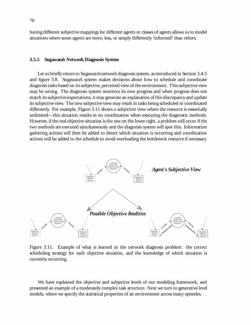
70

having different subjective mappings for different agents or classes of agents allows us to modelsituations where some agents are more, less, or simply differently ‘informed’ than others.

3.5.5 Sugawara’s Network Diagnosis System

Let us briefly return to Sugawara’s network diagnosis system, as introduced in Section 3.4.5and figure 3.8. Sugawara’s system makes decisions about how to schedule and coordinatediagnosis tasks based on its subjective, perceived view of the environment. This subjective viewmay be wrong. The diagnosis system monitors its own progress and when progress does notmatch its subjective expectations, it may generate an explanation of this discrepancy and updateits subjective view. The new subjective view may result in tasks being scheduled or coordinateddifferently. For example, Figure 3.11 shows a subjective view where the resource is essentiallyunlimited—this situation results in no coordination when executing the diagnostic methods.However, if the real objective situation is the one on the lower right, a problem will occur if thetwo methods are executed simultaneously and the diagnosis system will spot this. Informationgathering actions will then be added to detect which situation is occurring and coordinationactions will be added to the schedule to avoid overloading the bottleneck resource if necessary.

Agent's Subjective View

Possible Objective Realities

Diagostic Method Agent 5

Diagostic Method Agent 6

Limited Bandwidth

Communication Resource

U

ses(10

)

Uses(10)

Diagostic Method Agent 5

Diagostic Method Agent 6

Limited Bandwidth

Communication Resource

U

ses(10

)

Uses(10)

Diagostic Method Agent 5

Diagostic Method Agent 6

Limited Bandwidth

Communication Resource

U

ses(10

)

Lim

ited(1

5,50%

)

Uses(10)

Limited(15,50%)

Figure 3.11. Example of what is learned in the network diagnosis problem: the correctscheduling strategy for each objective situation, and the knowledge of which situation iscurrently occurring.

We have explained the objective and subjective levels of our modeling framework, andpresented an example of a moderately complex task structure. Next we turn to generative levelmodels, where we specify the statistical properties of an environment across many episodes.

71

3.6 TÆMS Generative Level Models and Framework Examples

3.6.1 The Generative Level

By using the objective and subjective levels of TÆMS we can model any individual situation;adding a generative level model allows us to go beyond that and determine what the expectedperformance of an algorithm is over a long period of time and many individual problemsolving episodes. A generative-level model can be viewed as a workload (episode) generator foran environment. In our work we have used statistical generative models of task inter-arrivaltimes (exponential distribution), amount of work in a task group (Poisson), task durations(exponential), and the likelihood of a particular non-local effect between two tasks (we’ll seemore of this in Chapters 5 and 6 [Decker and Lesser, 1993b, Decker and Lesser, 1993a,Garvey and Lesser, 1993]. Generative level statistical parameters can also be used by agentsin their subjective reasoning. For example, an agent may make control decisions based on itsknowledge of the expected duration of methods.

A generative level model can be constructed by careful analysis of the real environmentbeing modeled, or by observing the statistical properties of real episodes (if that is possible).Even when certain parameters of the real world are unknown, they can be made variables in themodel and then you can ask questions about how much they affect the things you care about.Our approach so far has been to verify our assumptions about the environment with simplestatistical approaches [Kleijnen, 1987]. Detailed model verification will be more importantwhen using our framework to optimize parameters in a real application, which is not a focus ofthis dissertation. In this dissertation we will focus on learning the general effects of parameterson a coordination algorithm (see Chapters 5 and 6).

An excellent way to proceed in building a generative model (the one we have used) is togather several detailed TÆMS objective and/or subjective task structures for specific episodes.These can be then examined to determine the obvious endogenous features of the episode thatare provided by the environment. For example, the number and lengths of tracks in DSNs; theset of tests ordered for patients in a hospital scheduling problem; arrival lateness and resourcefailure rates for an airport resource management problem. Developing a task structure forseveral episodes constrains and focuses the model-builder. Future work could examine thepossibility of inducing generative parameters from the observation of episodic task structures.

In our DSN model example, any single episode can be specified by listing the task groups,and what part of each task group was available to which agents, given the organizationalstructure. Our analyses are based on the statistical properties of episodes in this environment,not any single instance of an episode. The properties of the episodes in a DSN environment aresummarized by the tuple D =< A; �; r; o;T (l) > where A specifies the number of agents, �the expected number of task groups, r and o specify the structural portion of the organization bythe range of each agent and the overlap between agents19, and T (l) specifies the homogeneoustask group structure (as discussed in Sections 3.3 and 3.5.4). A particular episode in thisenvironment can be described by the tuple D =< T1(l1); : : : ;Tn(ln) > where n is a randomvariable drawn from a Poisson distribution with an expected value of �, and the li are generatedas described in Section 3.3. If we were to extend this generative model to cover every featurewe added to the objective and subjective models in Sections 3.3 and 3.5.4, we would need toadd the likelihood of a sensor being faulty (noisy), the likelihood of a ghost track, etc.

19We also assume the agents start in a square geometry, i.e, 4 agents in a 2�2 square, 25 agents arranged 5�5.

72

3.6.2 The TÆMS Simulator Generator

In order to test coordination and scheduling algorithms in general environments, the TÆMS

simulator has a random task structure generator. Describing this generator will give you anexample of how generative-level models of abstract task environments can be constructed. Thisgenerator does not generate structures from a “real” application environment; the structures itgenerates are quite abstract. When working with TÆMS on a particular application (such as inthe DSN problem in the next chapter), we do not use this random generator, but rather onecrafted to match the specific environment. These random, abstract environments are useful forgeneral experimentation and performance analysis of scheduling and coordination algorithms.

The random environment generator has three parts: specifying general environmentalparameters such as the inter-agent communication delay, specifying a generative subjectivetemplate, and specifying the potential classes of task groups (generative objective templates).

The default generative subjective template takes a list of agent names and a simpleprobability poverlaps for the chance of overlapping methods. For each objective methodgenerated and for each other agent, there is a poverlaps chance that the agent will have anoverlapping method. All objective values are passed unchanged to the agents. Agents whoexecute information-gathering actions will receive information on all methods executable bythem, and all parents of those methods, recursively. The default generative subjective templateguarantees no other subjective properties.

A random environment will consist of one generative subjective template and a list ofgenerative objective templates (one for each potential class of task groups). Each generativeobjective template takes the following parameters:

branching-factor: The average number of children of a task in the task structure. Specified asthe mean (equals the variance) of a Poisson distribution.

depth: The average depth of the task structure (not counting the leaf methods). Specified asthe mean (equals the variance) of a Poisson distribution.

duration: The average initial duration (d0) of a method. Specified as the mean of anexponential distribution.

max-quality: The average initial max-quality (q0) of a method. Specified as the mean of anexponential distribution.

QAF: The distribution of potential Quality Accumulation Functions for tasks. Specified as acustom discrete distribution such as “50% Min, 50% Max”.

Deadline: Deadline tightness. The deadline for the task group is set to �ESAET + � whereESAET is the Estimated Single Agent Execution Time of the actual instantiated taskgroup, and � and � are the specified parameters. The calculation of ESAET is only anestimate because it ignores non-local effects.

Inter-Arrival-Time: The mean time between arrivals of instances of this task group class.Specified as the mean of an exponential distribution.

Redundant-QAF: The Quality Accumulation Function to use when combining overlappingmethods. If the methods are redundant, then MAX is an appropriate choice.

73

The TÆMS random structure generator also allows the specifications of certain ‘patterns’ ofrelationships on top of this basic structure. These patterns have parameters that are in additionto the generative objective template parameters just mentioned:

Random-Relations: Generates hard and soft relationships with some probability but in noparticular pattern. Hard relationships are always generated across siblings to preventloops (i.e., pick a sibling, test if it should be hard-related to any of the remaining siblings,then pick one of the remaining siblings and continue until no siblings are left). Therandom-relations pattern takes two new parameters:

hard-rels: A discrete distribution of potential relationships or NIL for no relationship.For example, “10% enables, 90% NIL”.

soft-rels: A discrete distribution of potential relationships or NIL for no relationship.For example, “20% facilitates, 10% hinders, 70% NIL”.

cleanup-methods: One possible environmental pattern (seen in the DVMT) is the presence ofa method that must be done at the completion of other subtasks of an AND task. TheVTM’s and VCM in Figure 3.2 are a few examples. This pattern generates such ‘cleanupmethods’ that are subtasks to an AND task and that are enabled by all the other subtasksof the AND task. The cleanup-methods pattern takes one new parameter:

cleanup-prob: The simple probability that such a method is actually generated.

Fast-fallback-at-leaves: In environments where design-to-time scheduling is useful, there areoften multiple ways of achieving some task that do not all have to be done. A quick-and-dirty method that can be executed when the agent is under severe time pressure is calleda ‘fast fallback method’. This pattern generates such methods as alternatives to existing‘regular’ methods at the leaves of the task structure. The fast-fallback-at-leaves patterntakes three new parameters:

fast-fallback-prob: The probability that a given method will have a fast-fallback alter-native.

fast-fallback-percentage: A specification of the time/quality tradeoff represented by thefast fallback method (how much faster and how much less quality).

fast-fallback-hinders-p: Often doing something the quick and dirty way will end uphurting you later on (for example, the hindering precedence relationship in theDVMT structure of Figure 3.7). This parameter, if not NIL, specifies theparameters to a hinders relationship between the the fast fallback method andits parent task’s parent task.

3.6.3 Examples

In this section I will present several examples of TÆMS models for several quite differentenvironments. This will demonstrate the flexibility of the approach, and allow me to discuss theimpact of each task environment on coordination issues (even with relatively sketchy models).The distributed sensor network model, which has been the focus of the examples in the lastthree chapters, will not be repeated here.

74

3.6.3.1 Hospital Patient Scheduling

This description is from an actual case study [Ow et al., 1989]:

Patients in General Hospital reside in units that are organized by branches of medicine,such as orthopedics or neurosurgery. Each day, physicians request certain tests and/ortherapy to be performed as a part of the diagnosis and treatment of a patient. [: : : ] Testsare performed by separate, independent, and distally located ancillary departments inthe hospital. The radiology department, for example, provides X-ray services and mayreceive requests from a number of different units in the hospital.

min task with qualityaccrual function min

subtask relationship

enables relationship

method (executable task)type

min

Barium X-RayPhysicalTherapy

min

DrawBlood

Test 1

Test 2

min

min

min min min min min

min

Nursing Unit 1

min

min min min min min

min

min

Barium X-Ray

Ancillary 1 Ancillary 2 Ancillary 3

min task already communicatedto ancillary

requires delay

inhibits

Nursing Unit 2

resource

resource-constrains

Patient1

Patient

1Patient

2

Figure 3.12. High-level, objective task structure and subjective views for a typical hospitalpatient scheduling episode. The top task in each ancillary is really the same objective entity asthe unit task it is linked to in the diagram.

Furthermore, each test may interact with other tests in relationships such as enables,requires�delay (must be performed after), and inhibits (test A’s performance invalidates testB’s result if A is performed during specified time period relative to B). Note that the unitsecretaries (as scheduling agents) try to minimize the patients’ stays in the hospital, while theancillary secretaries (as scheduling agents) try to maximize equipment use (throughput) andminimize setup times.

A generative level model of this environment would focus on the mean time betweenpatient arrivals, and the number and distribution of patient tests. Other generative parameterswould include the specification of the ‘agents’ in this environment: the number of nursing unitsand the number and type of ancillaries and their associated resources (i.e., how many X-raymachines can be used in parallel by ancillary 1). Thus an episode generator for Ow’s hospitalwould have a fixed number of nursing units and ancillaries, and a fixed set of test templatescorresponding to taking X-rays, physical therapy, blood tests, etc. These templates would also

75

contain duration distributions on how long it takes to take the x-ray, etc. Then, we wouldpostulate an arrival rate for patients, and for each patient a distribution of tests (instantiatedfrom the set of templates). Thus when each patient arrives, linked to that patient is a uniquetask structure of what needs to be done to that patient.

Figure 3.12 shows a hand-generated example objective TÆMS task structure correspondingto an episode in this domain, and the subjective views of the unit and ancillary schedulingagents after four tests have been ordered. I use min (AND) to represent quality accrual becausein general neither the nursing units nor ancillaries can change the doctor’s orders—all testsmust be done as prescribed. This figure is different from the earlier one in that it explicitlyrepresents the patient as a non-sharable resource (resource�constrains represents the pair ofNLE’s uses and limits). Note that the patient is not needed for all portions of all tests (i.e., theblood work after the blood samples have been drawn). Also note that I have not represented thepatient’s travel times in any way—this is an important difference from the airport environmentdescribed in the next section. The reason for not representing this is that the scale of theproblem is such that patient travel time can be fixed beforehand (auxiliaries can assume thatthe patients will be delivered from their rooms rather than from other auxiliaries). I will go sofar as to point out the future implications of this downplay of travel times—this hospital willhave to change its organization, i.e. its coordination and scheduling mechanisms, if it has toface significant travel delays with more than one ancillary. This could happen if, for example, itis a smaller hospital and cannot afford its own MR scanner or CAT scanner and doctors taketo prescribing MR and CAT scans at another hospital. Patients requiring both MR and CATscans now have a significant facilitates effect in their task structures to do both scans nearlyconsecutively (potentially affecting the coordination structures of both hospitals).

The requires�delay relationship says that a certain amount � of time must pass afterexecuting one method before the second is enabled. I’ll repeat the definition I gave in the firstchapter here:

requires�delay(Ta;M; t; d; q; �) =

([d0(M); 0] Start(M) < Finish(Ta) + �

[d0(M);q0(M)] Start(M) � Finish(Ta) + �(3.15)

Examining the hospital’s current coordination structure is enlightening because it shows amismatch between the structure and the current hospital environment (this mismatch havingtriggered the study in the first place). From this mismatch we can guess at how the environmenthas changed over time, assuming that the current hospital structure was in fact a good structurewhen it was originally put into place.20

The current hospital structure is described by Ow as follows [Ow et al., 1989]:

After receiving a request from a physician, the unit secretary conveys the test requestto the secretary of the relevant ancillary department. In turn, the ancillary secretarydetermined the appropriate time for the test to be run. The unit secretary is notifiedimmediately prior to that scheduled time slot and not sooner. The actual time thepatient is scheduled is known only to the ancillary secretary (i.e., it is not relayed backto the requesting unit). Since each ancillary schedules independently (and withoutknowledge) of all other ancillaries, conflicts arise when a patient is scheduled inoverlapping (or nearly overlapping) time slots in different ancillaries. Such conflicts

20Ow calls this the sympathetic structure[Ow et al., 1989].

76

must be resolved by the unit secretaries. However, as the unit secretaries are madeaware of the scheduled ancillary times only when the request to “deliver” the patientcomes from the ancillary, little slack time remains to resolve scheduling conflicts anddelays, This can disrupt the care of the patient.21

While this structure seems sorely lacking when compared to the current environment, itmay at one time have been a reasonable, low overhead arrangement. It may be that in the pastdoctors ordered fewer tests on less complex ancillary equipment (there has been quite an ex-plosion in medical technology in the last decade) and (concomitantly) interfering relationshipsbetween these technologies. The structure is adapted for a different task environment.

Ow, et al. describe a new set of coordination mechanisms, using computer support, thatare better adapted to the hospital’s current task environment. Two types of computer agentsare defined—a unit subsystem that collects, disseminates, and monitors the test requests andresulting schedules for the patients in a unit, and an ancillary subsystem that receives testrequests from the unit subsystems and schedules them. Two communication protocols rest onthis structure:

Primary: The unit subsystems inform the appropriate ancillary about the test request (trans-mitting part of the task structure). The request includes a soft deadline (the ‘flow duedate’) for the task. The ancillary will schedule the test immediately, using a sharedprimary performance criteria of not missing the deadline, and secondary local criteriasuch as minimizing setups, maximizing throughput, etc. All other criteria being equal,the ancillary picks the earliest slot. As soon as the slot is chosen, the scheduled slot(what I will later call a commitment in the discussion of GPGP in Chapters 5 and 6) iscommunicated back to the unit subsystem.

Secondary: As soon as a slot is scheduled for a patient at an ancillary, the slot (commitment)is broadcast to all other ancillaries, thus effectively blocking that slot from considerationby the other ancillaries for any tests on that patient (as indicated in the diagram by theresource�constrains relationships.

One thing to note about this new system is that it does not explicitly handle interactionsbetween tests at different ancillaries. The GPGP family of coordination algorithms (Chapters 5and 6) could be configured to respond to these interactions as well as eliminate broadcastcommunication.

3.6.3.2 Airport Resource Management

The UMASS ARM (Airport Resource Management [Hildum, 1994]) and Dis-ARM(Distributed ARM [Neiman et al., 1994]) systems solve airport ground service schedulingproblems. The function of such systems is to ensure that each airport flight receives requiredground servicing (gate assignment, baggage handling, catering, fuel, cleaning, etc.) in time tomeet its arrival and departure deadlines [Neiman et al., 1994]:

21Additional problems may also ensue. For example, in some cases the sequence of multiple tests are important—a wrong sequence can result in patient stay delays as the residual effects of one test may influence the earliest starttime of another test [Ow et al., 1989].

77

The supplying of a resource is usually a multi-step task consisting of setup, travel,and servicing actions. Each resource task is a subtask of the airplane servicingsupertask. There is considerable parallelism in the task structure: many tasks canbe done simultaneously. However, the choice of certain resource assignments can oftenconstrain the start and end times of other tasks. For example, selection of a specificarrival gate for a plane may limit the choice of servicing vehicles due to transit time fromtheir previous servicing locations and may limit refueling options due to the presence orlack of underground fuel tanks at that gate. For this reason, all resources of a specifictype can not be considered interchangeable in the AGSS domain.

The generative model for this environment includes the nominal flight schedule, a modelof the errors in this schedule (i.e., late arrival times), and the airport’s resources (assuming allplanes will need the same set of services). An episode is a 24-hour time period including theinitial, nominal flight schedule. Another possible addition to the generative model are failurerates for the servicing resources. Because the nominal flight schedule for the airport is fixedahead of time, generating an episode mostly concerns variations in arrival time (usually delays)and equipment breakdowns. Each arriving flight spawns a task group to service that flight.

Figure 3.13 shows the objective task structure for a small episode with two gates, two fueltrucks, and two baggage trucks. Gate 2 has an underground fuel tank, and thus enables localfuel delivery without needed a fuel truck. Slightly unusual relationships hold between using agate and servicing the plane, because the gate must be held for the entire time of servicing (asopposed to a strict sequencing like enables). The subjective information available to any agentis the same, except for the arrival times of task groups (flights) in the future, which are onlytentative.

Tmin

task with qualityaccrual function min

subtask relationship

enables

method (executable task)

starts-before

agent

ServicePlane

UseGate

Fuel Baggage

NWA451

G1 G2

F1 F2Local B1 B2

ServicePlane

UseGate

Fuel Baggage

NWA118

G1 G2

F1 F2Local B1 B2

Gate1

Gate2

Fuel1

Fuel2

Bags1

Bags2

Gate1

allows-finish

resource-constrains

resource

Figure 3.13. Objective task structure for a small airport resource management episode.

Notice the differences between this structure and the hospital structure. Resources aremuch more important here, and connect much more of the substructures to one another.Much of this comes out of the necessity to represent the effect of equipment travel times that

78

are not represented in the hospital case (the point is not that ‘equipment doesn’t travel in thehospital’ but that the travel times of the patients can be standardized—an important classicalcoordination technique). Travel times, however, cause every action taken by a resource (suchas a fuel truck) to be related to every other action in a complex way, changing the effects ateach potential successive action (I’ll talk about this again in Section 7.5 below).

This strongly connected structure thus impacts the potential coordination mechanismsused. For example, in ARM, and in real airports, this scheduling is done in a centralizedmanner for a fixed set of resources (although one might consider resources such as baggagetrucks as ‘agents’, in such a system these agents are slaves that only obey the commands of thecentral coordinator—similar to the bulldozers in Phoenix[Cohen et al., 1989]).

Such a centralized scheduling process is obviously expensive and complex in terms ofcomputation. The Dis-ARM project [Neiman et al., 1994] looks to provide performanceimprovements over a centralized system by using multiple schedulers. The subjective view ofthe problem for each scheduler is considerably simplified by assigning each scheduler exclusivecontrol of certain resources (for example, each scheduler could get one airport concourse ofgates and a commensurate number of fuel and baggage trucks). Each scheduler tries to locallyschedule the services for planes arriving in its concourse. The problem at each agent thenbecomes considerably simpler because it has been separated from the similar problems at otheragents’ concourses, and the agents can solve the problems in parallel as well. The downside isthat the totally separate solutions are potentially more wasteful of resources. To combat this,the Dis-ARM system allows agents to lend resources to one another—note however that eachlending act will connect initially unrelated task groups through resource relationships and makeeach agent’s scheduling that much harder.

Other solutions are also suggested by the task structure. For example, since the servicesprovided to each plane are already standardized, one could schedule the services at a constantheadway (or one keyed to the business pattern, i.e., closer headway during the morning andevening rush times). Thus pre-scheduled and fixed slots would be established, and when a planearrives (or soon before) it would be assigned to the next available slot (and associated gate).This technique removes the uncertainty in plane arrivals from the system (but is probably notused by airports because they wish for gate assignments to be made as early as possible, bothfor customers and for automated baggage handling). Another solution would be similar to theDis-ARM structure; basically the corporate division organizational form—rather than directnegotiation, each scheduler (division) would apply for resources through a centralized ‘frontoffice’ (which in turn centralizes all the rapidly changing information about the resources). Amodification to this structure is a matrix organization where separate agents keep track of eachclass of resources (i.e., a baggage truck agent, a fuel truck agent, etc.) and then other agents areresponsible for servicing the flights, drawing resources from the resource-class pools [Sycara etal., 1991].

3.6.3.3 Internet Information Gathering

Another task environment mentioned briefly in the overview of this thesis was distributedinformation gathering. The Internet, as well as several popular commercial services, growby leaps and bounds daily, providing rich and varied sources of information. Quickly andefficiently retrieving this information can be viewed as a set of interrelated tasks in an uncertain

79

and dynamic environment. The same piece of data can be available via many different methods,and at many different locations; at any point of time only some of those locations are acessablethrough some subset of methods. It is extremely common nowadays for one to know preciselywhere a certain answer can be found but for one to have to undertake a time-consumingsequential search to find a currently available resource and access method. Within a singlequery, multiple agents could search in multiple locations in parallel and coordinate theiractions when it was useful. For example, the results of work by one agent may suggest the needfor some of the existing agents to gather additional information, or it might suggest the needfor a new division of tasks among the agents [Oates et al., 1994].

Generative level information in this task environment includes the frequencies and typesof queries (are the agents beholden to individuals, or are they available to the network, whichwould result in very different usage patterns). It also includes information about the dynamicsof the environment: how frequently do connections or links to physical information sourceschange, how often are the physical sources available, how often does the information on thosesources change? How often are new physical sources being added?

resource-constrains

physical resource

Tmin

task with qualityaccrual function min

subtask relationship

method (executable task)agent

R1

MacQuery

Tidbits LibraryInfoMac

query specification

WAIS FTP

ftp.tidbits.com

mirror 1tidbits.SRC

max

sour

ce sp

ecifi

catio

n

MovieQuery

BillDB

WAIS HTTP

BillDB.SRC

TMCCM

Figure 3.14. High-level, objective task structure for a two independent queries that resolve atone point to a single machine.

Figure 3.14 shows part of an objective level description of an example episode. Here twoqueries are being made—one about Macintosh information and one about movies. The Macquery might encompass several general sources of Mac information—the TidBits electronicnewsletter, Info-Mac and other electronic file archives, Usenet newsgroups, and even standardlibrary article searches. This particular query might be constructed by the interaction of a humanuser and a persistent Mac query intelligent agent. The task of searching each information sourcecan be broken down into the different possible access methods for that source (e.g., WAIS, FTP,HTTP, a special-purpose agent that can use telnet to access a class of library databases, etc.).Each access method may still imply multiple physical resources (for example TidBits back issuescan be found both at the mother site ftp.tidbits.com and at various mirrors of that site. Workdone retrieving from mirror sites is redundant in the TÆMS sense—but which sites are likely to

80

be operating at all? How fast will they be? Are they accepting connections?22 One can imaginethe enforcement of user performance criteria on the agents carrying out these tasks. One usermight want a (not necessarily complete) answer immediately, another might be willing to waitfor the agents to find the ‘best’ answer they can find. Queries might be continuous ‘profiles’for information to be retrieved now and in the future as it becomes available.

Another point to note about Figure 3.14 is the presence of shared resources linkingotherwise unrelated queries. In this example the shared physical resource is Thinking Machines’CM5 WAIS server,which stores many example WAIS databases. Other similar examples includepopular mirror and archive sites like uunet.uu.net and wuarchive.wustl.edu.

Tmin

task with qualityaccrual function min

subtask relationship

method (executable task)

enables

facilitates

agentReview

Library

InfoMac

Tidbits

WAIS FTP

ftp.tidbits.com

mirror 1tidbits.SRC

max

Online Paper

News

Seller

Retrieve

Tidbits

Locate

FaxOnline

fromlibrary(humanagent!)

fromseller

frommagazine

($)

fromUncover

($)Uncover

pac.carl.orgxyzzy.com

Figure 3.15. Mid-level, objective task structure for a single query for a review of a Macintoshproduct showing intra-query relationships.

Figure 3.15 shows more detail from a particular Macintosh query episode for a review ofsome Mac software product. Such reviews can be found both in online forms and in whatwere originally published paper forms (but which may now be online as well). A user mayperhaps view truly published product information as being of higher quality. Online productinformation might be found in the review portion of the TidBits newsletter, or in collectedproduct information in the Info-Mac archives, or in exchanges about a product in UsenetNews. Finding paper reviews of a product can be reduced to locating a citation and then theactual article itself. TidBits contains the table of contents of the popular Macintosh magazines;some magazines are indexed by free periodical indices such as Uncover; sometimes the sellerof a product will both have information available on the net and citations of reviews of theirproduct. Once a citation is found, retrieval can be by hand or from online sources (but almostall of these will cost money). Note that some parts of this structure facilitate others, e.g., having

22These are all generative level questions.

81

used Uncover to come up with a citation it is very easy to have the article faxed to you at aprice.

The task structure of this environment lends itself to a great deal of parallelism since a lotof work can be done in parallel and the interrelationships are relatively few and fixed. On theother hand, efficient planning for search according to a users preferences (e.g., quick response?best answer?) make the coordination problem more one of intelligent task decomposition.

3.6.3.4 Pilot’s Associate

The global coherence problems we would like to address occur in many systems otherthan the DVMT, such as the Pilot’s Associate (PA) system [Smith and Broadwell, 1987],where situations occur that cause potentially complex and dynamically changing coordinationrelationships to appear between goals that are spread over several agents. Each agent in thePilot’s Associate system has subtasks that other agents must fulfill, and receives tasks from otheragents that only it can fulfill.

For example, assume that we are in a tactical situation, so the tactical planner is in control(see Figure 3.16). It has two ordered subtasks: turn on the active sensors (request to situationassessment), and get a detailed route of the plane’s movements during the tactical maneuver(request to the mission planner). Turning on active sensors causes a plane to become atransmitter, and thus become easily detected (most of the time the plane uses passive sensors).Since this is dangerous, the situation assessment agent will ask the pilot-vehicle interface (PVI)to ask for pilot confirmation of the use of active sensors. The pilot, upon seeing the request,asks the PVI to plot the escape route of the plane on the screen in case things go wrong. ThePVI passes this task to the mission planner.

Meanwhile, the tactical planner has asked the mission planner to produce the detailedroute for the tactical maneuver. Which task does the mission planner act on first? From a localview, it may perhaps do the tactical planner request first because the tactical planner tasks are ahigh priority. But from a global perspective, we see that unless the mission planner plans theescape route, which is needed by the pilot in order to authorize turning on the active sensors,which is needed for the tactical planner to do its job, the whole system performance goal ofhandling the tactical situation is in jeopardy. Hence the mission planner should do the escaperoute plan first.

Although I do not describe GPGP in detail until Chapter 5, let me briefly describe thisscenario in those terms. There will be an overall deadline on the ‘respond to tactical situation’task, which will be inherited by the ‘plan tactical route’ subtask. The enables relation between‘get pilot confirmation’ and ‘do it’ (pinging the active sensors) could trigger a GPGP mechanismto place an earlier deadline on the ‘get pilot confirmation’ task when it is communicated to thePilot Vehicle Interface. The task ‘show escape route’, based on this, would also have an earlierdeadline, and thus ‘plan escape route’ would have an earlier deadline (earlier than ‘plan tacticalroute’) as well. Thus the Mission Planner obtains the necessary information with which toschedule the two tasks. If the time to do both tasks is more than the earlier deadline and lessthan the later deadline, then the scheduler can only rationally choose to do ‘plan escape route’first.

82

Planescaperoute

Plantacticalroute

Respond totactical

situation

Turn onactive

sensors

Showescaperoute

Do It!

min task with qualityaccrual function min

subtask relationship

enables relationship

method (executable task)type

Pilot Vehicle Interface

Mission Planner

Situation Assessment

Tactical Planner

Get pilotconfirmation

Pilot

Figure 3.16. Dynamic Situations in Pilot’s Associate. All tasks accrue quality with Min (AND).

3.7 Summary

This chapter discussed a characterization of the features and model of the processesin computationally intensive task environments called TÆMS (Task Analysis, EnvironmentModeling, and Simulation). No characterization currently exists that formally captures therange of features, processes, and especially interrelationships that occur in computationallyintensive task environments. In the simplest terms, a TÆMS model of a task environmentspecifies what actions are available to agents and how those actions relate to one another. Thisframework is useful not only for the study of coordination (which will be the subject of thenext two chapters) and other related CDPS behaviors (for example, our brief discussion ofnegotiation with respect to Dis-ARM), but also for the study of the planning and schedulingof computation in realistic real-time or parallel task environments [Garvey et al., 1993,Garvey and Lesser, 1993]. The contribution of TÆMS itself is really as a base from whichto work—a way to describe an environment carefully, as shown in the examples at the end ofthe last section. It is also a way to specify the behavior of an agent when you are designing it’scontrol mechanisms, as I will show with GPGP in Chapter 5. Many other things that can bedone with TÆMS including analysis and simulation, will be described in the following chapters.

The work described here is of course not without limitations. Some of these are currently

83

being addressed in follow-up work. TÆMS describes an environment from three differentviewpoints, but this dissertation concentrates mostly on the objective viewpoint. It does notdeal with the various representations of uncertainty that might be in an agent’s subjectiveview—we are currently working on this aspect. The generative models in this dissertationare constructed from a statistical viewpoint—an episode can be characterized by the values ofseveral random variables. While this is far better than using a set of single-instance examples, itmay not be appropriate for dynamic environments, where the task structure itself is changingdramatically over time. More complex models of generation may be needed. For example,generation might be modeled by a set of meta-agents.

Furthermore, especially when modeling human agents and organizations, we only addresswhat might be called “certain specified uncertainty” [Anderton, 1994]—bounded uncertaintyabout known things. But in real human organizations, often external forces change the verystructure of the environment in essentially unpredictable ways. The very factors that influencebehavior, the measures of performance, etc., might change out from under the agent withno prior warning (or bounding of the uncertainty surrounding these matters). We’ll discussthis more in Chapter 2. Another problem is if any such general framework could achieve anexternal validity that doesn’t require constant re-verification in a new domain. While this seemspossible for computational environments, it doesn’t seem possible for human systems.

The TÆMS representation of task environments is abstract, with the smallest units corre-sponding to schedulable actions and their relationships (what that means will depend on theenvironment being modeled—anything from an indivisible set of real-time tasks to an abstractorganizational unit action). The TÆMS representation is not intended as a schedule or planrepresentation, although it provides much of the information that would go into such uses.TÆMS has many dynamic features including:

� dynamic stochastic arrival of whole or partial task structures,

� dynamic changes to interrelated task durations and qualities caused by the actions ofother agents and stochastic environmental processes

� dynamic changes to the agents’ local views as time progresses and caused by local andnon-local actions

The concept of agency in TÆMS is based on simple notions of execution, communication,and information gathering (collectively, actions). An agent is a locus of belief (state) and action.By separating the notion of agency from the model of task environments, we did not haveto subscribe to particular agent architectures (which one would assume will be adapted tothe task environment at hand). TÆMS exists happily alongside blackboard systems, Shoham’sagent oriented programs, or other agent architectures. Such a conception is unique amongcomputational approaches. We’ll talk about blackboard-style (DVMT) agents in the nextsection, and you’ll see our use of an architecture similar to Shoham’s agent oriented programsin Chapter 5 (GPGP).

The framework is general in that it is based on abstract features, applicable to manydomains. It is not a model of a specific domain, such as sensor interpretation or fire fighting.We showed models of several different environments and episodes in this chapter; we’ll expandon the simple distributed sensor network model in the next chapter.

84

A unique feature of the TÆMS framework is the direct representation of interrelationshipsbetween tasks beyond resource and precedence constraints. Coordination relationships arecrucial to design and analysis of coordination mechanisms, as you will see in chapters 5and 6. TÆMS allows the formal functional specification of arbitrary task interrelationships;Section 3.4.3.1 described a useful basic subset.

Finally, this chapter demonstrated, as promised, that TÆMS models are built in threelayers—objective, subjective, and generative. This allows us to capture the single probleminstances that have appeared in many previous non-formal approaches to CDPS systems (i.e.the DVMT, hospital scheduling, and other examples in the final section). We can also useit to look at wider classes of problems with stochastically varying features from a statisticalperspective—and that is exactly the subject of the next chapter.

C H A P T E R 4

DESIGN AND ANALYSIS OF COORDINATION ALGORITHMS: ATASK ENVIRONMENT MODEL FOR A SIMPLE DSN

ENVIRONMENT

Now I know a problem that physics won’t resolve: : : I know a color that acid won’t dissolve: : : a place that’s just too far I think for us to go

Now is it wise to have a hope so strongfor real-time answers to real-world wrongs?

— Game Theory, Distortion:“Nine Lives to Rigel Five”, 1984

In the previous three chapters I described the TÆMS framework and several examplemodels, including one of a simple Distributed Sensor Network (DSN) environment. Thischapter takes this model and uses it to analyze the DSN problem in some depth. Previousapproaches to analyzing organizations in distributed sensor networks have either not focusedon the effectiveness of the organization [Davis and Smith, 1983, Pavlin, 1983], or have onlyanalyzed organizational effectiveness in particular, single-instance examples [Durfee et al.,1987]. Others work has focussed on analysis in general situations, but is extremely abstract[Malone, 1987]. Sen has done an analysis similar in spirit to that presented here, but in adifferent domain (meeting scheduling for two agents)[Sen and Durfee, 1994]. I will develop andtest mathematical expressions for the important TÆMS characteristics of objective episodes in theDSN environment, and use these expressions to develop and analyze coordination algorithmsfor agents in this environment. By the end of this chapter I will have developed expressions forthe primary performance criteria in this environment—termination time—for two differentcoordination algorithms. I validate these mathematical models by using simulations.

A dynamic organization is one in which the responsibilities of agents can be reassignedbased on a developing view of the problem at hand. Agents that have a dynamic organizationhave the option of meta-level communication—communicating about the current state ofproblem solving as opposed to communicating about solving the problem itself. Due to theuncertainties explicitly represented in the TÆMS task environment model, there may not bea clear performance tradeoff between static and dynamic organizational structures in everyenvironment.

This chapter will serve as a concrete example of the impact of environmental differenceson coordination algorithms. Although I will discuss three different algorithms and implementtwo of them, no one algorithm will be the ‘best’, even statistically, for all DSN environments.If variance in an environment is large enough, it will behoove the agents to use meta-levelcommunication to build a dynamic organization that, as Stinchcombe puts it, expands towardthe earliest available information that resolves uncertainties in the current environment, allowingthe agents to then create an efficient organization for the situation.

86

4.1 Task Environment Simulation

In the next section, we will test the model we are developing against a simulation of DSNproblem solving. Each simulated DSN episode will take place on a grid where the conceptsof length and size correspond directly to physical distances. For example, Figure 4.1 illustratesseveral simple organizations imposed on such a grid in our simulation.

In the simulation we assume that each vehicle is sensed at discrete integer locations (as inthe DVMT), randomly entering on one edge and leaving on any other edge. Between thesepoints the vehicle travels along a track moving either horizontally, vertically, or diagonally eachtime unit using a simple DDA line-drawing algorithm (see Figure 4.6). In an 18 � 18 grid,the (empirical) average length of a track is 14 units—the actual length of any one track willrange from 2 to 19 units and is not distributed normally. Given the organization (r, o, and A,and the geometry), we can calculate what locations are seen by the sensors of each agent. Thisinformation can then be used along with the locations traveled by each vehicle to determinewhat part of each task group is initially available to each agent. In general, no agent will seeall the parts of a complete task group (track). Section 4.5 will detail what the structure of eachtask group is for the DSN simulation.

r=13

o=8

A=4

r=5

o=4

A=196

r=11

o=4

A=4

Figure 4.1. Examples of DSN organizations on an 18 � 18 grid

Our TÆMS generative level model of this process was discussed back in Section 3.3.The properties of the episodes in a DSN environment are summarized by the tuple D =<A; �; r; o;T (l) > where A specifies the variable number of agents, � the expected numberof task groups, r and o specify the variable structural portion of the organization by therange of each agent and the overlap between agents, and T (l) specifies a template for thestructure of each task group. A particular episode in this environment can be described by thetuple D =< T1(l1); : : : ;Tn(ln) >, where n is a random variable generated from a Poissondistribution with location parameter (central tendency) of �. The li are generated by theprocess explained above.

This specification is applicable to other interesting environments. For example: each taskgroup may comprise several different types of subtasks; each agent may only respond to acertain type of subtask (its ‘range’); multiple agents may respond to the same types (‘overlap’).In general, the parameters of ‘range’ and ‘overlap’ can be multidimensional.

87

4.2 Expected Number of Sensor Subtasks

When a system of agents is confronted by a particular DSN problem-solving episode, eachagent will sense, or ‘see’ 1 a certain amount of low level data associated with the tracks of vehiclesthat moved through the agent’s sensed area. In order to analyze the performance of a particularorganization, we will want to know (a priori) what proportion of each task group each agentis likely to process. There will be some upper limit on this proportion (related to the agent’srange r), and sometimes the agent will process less than this upper limit. Especially in staticorganizational structures where tasks are not exchanged, the termination of the system as awhole can be tied to the completion of all tasks at the most heavily loaded agent. Normally, wewould use the average part of a task group to be seen, but since the focus of our analysis is thetermination of problem solving, we need to examine the expected maximum portion of a taskgroup to be seen. This section will develop an equation for the expected maximum workloadat an agent by counting the expected number of low-level sensor subtasks (each individuallyassociated with a sensed vehicle location) that the maximally loaded agent will have.

The amount of a single task group seen by an agent (which is the same as the numberof sensor subtasks in the DSN example) can be viewed as a random variable S with aprobability density function and corresponding cumulative distribution function. In the DSNenvironment, S is discrete, and its probability function (determined empirically2) is heavilyweighted toward r (the maximum). To simplify the analysis, instead of letting S correspondto the number of subtasks in a single task group seen by an agent, let’s create a new randomvariableS that we have equal 1 if the agent sees the maximum amount, and 0 otherwise. NowShas a Bernoulli (coin-tossing) distribution with parameter p corresponding to the chance of anagent seeing the maximum amount r of a task group.3 Let’s assume we know that N � n is thenumber of task groups at the maximally loaded agent, and that on average a � A agents see asingle task group (we’ll remove these assumptions later). The number of times an agent sees themaximum out of N task groups (N coin flips) then has a binomial distribution (bN;p(s)). Weneed to know, given that a agents each flip N coins, what the distribution is of the maximumnumber of ‘heads’ any agent sees—this is called the binomial max order statistic, ga;N;p(s):4

bN;p(s) =�Ns

�ps(1� p)N�s [Pr [S = s]]

BN;p(s) =Ps

x=0 bN;p(x) [Pr [S � s]]

ga;N;p(s) = BN;p(s)a �BN;p(s� 1)a [Pr [S = s]]

The random variable S refers to any agent, and the new random variable S refers to themaximally loaded agent. Its probability function g(s) has a much steeper shape and largerexpected value than the binomial b(s) (see Figure 4.2). In the DSN example we have p = 0:55

and the amount of a task group seen when an agent does not see the maximum amount averagesr=2. In effect, we are modeling the sensor reception process by the simplification that when

1As is common with the DVMT, we will use “sensed” and “seen” interchangeably in this chapter.2I built a simulation and counted it in over 500 random episodes.3It is entirely possible to complete the analysis using the empirical, discrete distribution function, but it adds

little to the effectiveness of the model and needlessly complicates the discussion.4A more detailed derivation of this result is in our tech report.5Empirically determined through simulation as previously mentioned.

88

0

0.05

0.1

0.15

0.2

0.25

0.3

0.35

0.4

0.45

0 1 2 3 4 5 6 7 8 9 10

b10,0.5(s)

g2,10,0.5(s)

g5,10,0.5(s)

g10,10,0.5(s)

Prob

abili

ty

Value of ‘s’

Figure 4.2. A comparison of the probability distributions of the outcome of ‘heads’ in the actof flipping a coin 10 times (the binomial b10;0:5(s)) compared to the outcome of having 2, 5,or 10 agents flip 10 coins and taking the number of heads of the agent who flipped the mostheads (the max order statistics g2;10;0:5(s) through g10;10;0:5(s)).

the coin is heads we see the maximum r sensed data points, and when the coin is tails we seeonly r=2. Now we can convert back from the easy to analyze random variable S to the variablewe are really interested in, which I will call S, by the equation S = (rS + (r=2)(N � S)).The new random variable S models how many sensed data points are seen by the agent whosees the most complete tracks.

Remember that the definition of expected value is the sum of the product of the probabilityof a value and the value itself across all possible outcomes. In the case of S, the probabilityof any particular value is given by the appropriate max order statistic g that some agent sees s‘heads’, and the number of sensed data points is given by the function (rS + (r=2)(N � S))(again, when there were s ‘heads’). Therefore, the expected heaviest load seen by any agentwhen a agents seeN task groups with a probability p of seeing r and probability 1�p of seeingr=2 is:

E[SjN; a] =NXs=0

ga;N;p(s)(rs +r

2(N � s)) (4.1)

To reiterate: out of N task groups the maximally loaded agent sees the maximum r some S(a random variable) times, and the other (N � S) times it sees only r=2. Eq. 4.1 shows theexpected value of a new random variable S that indicates the number of sensor subtasks at themaximally loaded agent when there are N task groups in an episode. N is itself a randomvariable, we’ll look at its distribution in the next section.

89

Figure 4.3 shows the heaviest load actually observed and averaged over 1000 runs, plottedagainst the expected value, for n tracks and all square DSN organizations [2 � r � 10; 0 � o �r; 1 �

pA � 10; 1 � N � 10] (R2 = 0:98)6. The colors of the points refer to the value of r;

lighter grey corresponds to larger values of r.

Act

ual M

ax

10

20

30

40

10 20 30 40Estimated Max

Figure 4.3. Actual versus predicted heaviest load SN for various values of A, r, o, and N

4.2.1 Distribution of the Binomial Max Order Statistic

To expand on the formulae in Section 4.2, the amount of a single task group seen byan agent can be viewed as a random variable S with probability density function f(s) andcorresponding cumulative distribution function F (s). Let a be the number of agents thatinitially see part of a single task group. By elementary statistics, the density of the max orderstatistic Smax = max (S1; S2; : : : ; Sa) is ga(s) = aF (s)a�1f(s). The expected heaviestload then is

R r0 sga(s)ds. In the DSN environment, S is discrete, and its probability function

(determined empirically) is heavily weighted toward r (the maximum). To simplify the analysis,instead of letting S correspond to the number of subtasks in a single task group seen by anagent, we again introduce a new random variable S equal 1 if the agent sees the maximumamount, and 0 otherwise. Now S has a Bernoulli (coin-tossing) distribution with parameterp corresponding to the chance of an agent seeing the maximum amount r of a task group. Sthen corresponds to the number of times an agent sees the maximum r if the agent sees N taskgroups (tracks). S has a binomial distribution with parameters p and N . Now if a agents seeN task groups each, what is the distribution of S = max (S1;S2; : : : ;Sa)? This is the max

6R2 is the squared correlation coefficient, a measure of goodness of fit. It may be interpreted as the proportionof total variability in the observed data that is explained by the model.

90

order statistic for the binomial distribution, and because it is discrete, can be easily derived.The probability function and cumulative distribution function for the binomial distributionare:

bN;p(s) =�Ns

�ps(1 � p)N�s [Pr [S = s]]

BN;p(s) =Ps

x=0 bN;p(x) [Pr [S � s]]

If we assume each track is independent of the others, we can derive the cumulative distributionfunction:

Pr [S � s] = Pr [max (S1;S2; : : : ;Sa) � s]

= Pr [S1 � s] Pr [S2 � s] � � �Pr [Sa � s]

= BN;p(s)a

The probability function ga;N;p(s) = Pr [S = s] is then:

ga;N;p(s) = BN;p(s)a �BN;p(s� 1)a

4.3 Expected Number of Task Groups

Given the maximum number of task groups seen by an agent (N ), we can calculate theexpected heaviest agent load using Equation 4.1. But this begs the question of what is themaximum number of task groups an individual agent will see, given the actual (n) or expectednumber (�) that the entire system will see. The solution is similar—each agent either sees ordoes not see each of the n task groups, another binomial process. LetNi be the number of taskgroups sensed by agent i, with a binomial distribution of parameters n and q. If a is again thenumber of agents that see a single task group and A the total number of agents, then q = a=A,the probability that each agent will see a particular track (we’ll give an equation for a next). Bythe same derivation as in the last section, the max order statistic N has the probability functiongA;n;a=A(s), and expected value:

E[N jn; a] =nX

s=0

sgA;n;a=A(s) (4.2)

Figure 4.4 shows the actual mean value of the maximum number of tracks seen by an agentover 1000 runs of the DSN simulation, versus the predicted value, for n tracks and squareDSN organizations [2 � r � 10; 1 �

pA � 10; 1 � n � 10] without any overlap (R2 = 0:96)

4.4 Expected Number of Agents

The only remaining term we need to analyze before deriving an expression for systemperformance is a, the expected number of agents that will see a single task group. In general,a will depend on the total number of agents A and the organization (r and o). When there isonly one agent, it will see every task group (a = 1). When the agents overlap completely, everyagent sees every task group ([o = r] ! [a = A]). When the agents in a square environment

91

Act

ual M

ax N

umbe

r of

Tra

cks

Seen

0

1

2

3

4

5

6

7

8

9

10

0 1 2 3 4 5 6 7 8 9 10Predicted Maximum Number of Tracks

0

10

20

30

40

50

60

70

80

90

100

0 10 20 30 40 50 60 70 80 90 100

Act

ual n

umbe

r of

. age

nts

seei

ng a

tra

ck

Predicted number of agents to see a track

Figure 4.4. On the left, actual versus predicted maximum number of task groups (tracks) seenby any one agent for various r, A, and n. On the right, actual versus predicted average numberof agents seeing a single task group (track) for various r, o, and A.

do not overlap, a is approximatelypA. The relationship follows the ratio of the area solely

covered by an agent plus the area of the overlapping section, to the total area covered alone:

a = A( r

2+o2

2r2) (4.3)

Note that a is not a random variable, it is just derived directly from environmental parameters.Figure 4.4 shows a regression of the actual average value of a over 1000 runs verses the predictedvalue for all 630 DSN organizations [2 � r � 10; 0 � o � r; 1 �

pA � 10] (R2 = 0:98).

4.5 Work Involved in a Task Structure

So far we have derived models for the number of low-level sensor subtasks seen by the mostheavily loaded agent (S), the number of task groups seen by that agent (N ), and the averagenumber of agents to see a task group (a). Now we turn to the question of just how muchwork an agent that sees S sensed data points and N task groups has to do in order to solvethe problem at hand. Our model of the performance of the system as a whole is based on thestructure of the tasks involved. We will use TÆMS to describe this structure.

Let me briefly restate the basics of TÆMS from the previous chapter. The objective leveldescribes the essential structure of a particular problem-solving situation or instance over time.It focuses on how task interrelationships dynamically affect the quality and duration of each task.In this chapter we will concentrate only on duration as a performance metric. An individualtask that has no subtasks is called an executable method M and is the smallest schedulablechunk of work. The quality and duration of an agent’s performance on an individual task is afunction of the timing and choice of agent actions (‘local effects’), and possibly previous task

92

executions (‘non-local effects’). The basic purpose of the objective model is to formally specifyhow the execution and timing of tasks affect quality and duration.

Elsewhere in this dissertation we consider the case of facilitation, a non-local effect wherethe availability of a result from one task alters the quality and duration of another task, butthe non-communication of a result has no effect [Decker and Lesser, 1993a]. This chapterconsiders a different relationship, precedence. If task A precedes task B, then the maximumquality q(B; t) = 0 until A is completed and the result is available, when the maximum qualitywill change to the initial maximum quality q(B; t) = q0(B).

4.5.1 Execution Model

For this chapter we use an extremely simple model of execution (as described earlier inSection 3.5.3.1). Agents can perform three actions: method execution, communication, andinformation gathering. The control component of an agent determines the next action anagent will perform based on the agent’s current set of beliefs. A method execution action, ofmethodM , that is begun at time twill conclude at time t+d(M; t). An information gatheringaction has duration d0(I) and updates the agent’s set of beliefs with any new information inthe environment, for example, the arrival of data at the start of an episode, or communicationsfrom other agents. A communication action has duration d0(C) and, after a communicationdelay, makes information (such method execution results) available to other agents. The agenton the receiving side must perform an information gathering action before the communicationcan affect its local beliefs.

4.5.2 Simple Objective DSN Model

Recall from Chapter 3 that the summary of a DSN problem-solving environment was thetuple D =< A; �; r; o;T >. A particular episode in this environment can be described bythe tuple D =< A; r; o;T1; : : : ;Tn > where n is a random variable drawn from an unknowndistribution with location parameter (central tendency) of �. Note that we so far make almostno assumptions about this distribution; its characteristics will differ for different environments.For example, in the description of our DSN simulation early in Section 4.1 we noted thephysical process by which vehicle tracks were generated and that the length of the tracks wasnot normally distributed.

Each task group T i is associated with a track of length li and has the same basic objectivestructure, based on the DVMT (repeated here from Chapter 3):

� li Vehicle Location Methods (VLM’s) that represent processing raw signal data at a singlelocation to a single vehicle location hypothesis.

� li � 1 Vehicle Tracking Methods (VTM’s) that represent short tracks connecting theresults of the VLM at time t with the results of the VLM at time t+ 1.

� 1 Vehicle Track Completion Method (VCM) that represents merging all the VTM’stogether into a complete vehicle track hypothesis.

Non-local enables effects exist between each method at one level and the appropriate methodat the next level as shown in Figure 3.2—two VLMs enable each VTM, and all VTM’S enablethe lone VCM.

93

VTM

VCM

VLMVLM

VLMVLM

Tmin

VTM

VTM

TminT

min

Tmin

Tmin

method (executable task)

task with quality accrual function min

subtask relationship

enables relationship

Figure 4.5. Objective task structure associated with a single vehicle track.

If we assume that each VLM has initial duration d0(VLM) and each VTM has the initialduration d0(VTM), then we can see from the task structure that for each task group the totalexecution time taken by a single processor agent will be:

lid0(VLM) + (li � 1)d0(VTM) + d0(VCM) (4.4)

This task structure is a simplification of the real DVMT task structure. For example,there is no sensor noise (which will cause facilitation relationships between tasks, and there isno confusion caused by ‘ghost tracks’. Adding these features to the task structure can causeinteresting phenomena as was previously discussed in Section 3.5.4. That section explainedhow to add these features to this basic task structure using TÆMS.

4.6 Model Summary

This section has described our basic model of the DSN environment, beginning with thebasic parameters D =< A; �; r; o;T >. A particular episode in this environment can beindicated as D =< A; r; o;T1; : : : ;Tn >, where each of the n task groups has the structurementioned above. This section also developed expressions for S, the number of low-levelsensor subtasks (i.e., VLM’s) at the most heavily loaded agent, the number of task groups N atthe most heavily loaded agent, and the average number of agents a that see a single task group.Another way to look at these results is that we have derived the probability distributions of thesevariables, i.e., if the system of agents as a whole sees n total task groups, then the distributionsof N and S are:

Pr[N = N jn] = gA;n; aA(N) (4.5)

Pr[S = sjN = N ] = ga;N;0:5(s) (4.6)

S = (rS+ (r=2)(N � S)) (4.7)

Finally Eq. 4.4 derived the duration, or amount of processing work, involved in a single taskgroup from its structure.

94

In the next section we will combine these results with simple local scheduling andcoordination algorithms appropriate for static and dynamic organizations. This will allowus to describe the performance of a system of agents following one of these organizationalalgorithms in a particular episode or environment.

4.7 Static vs. Dynamic Organizational Structures: Reorganizing to Balance System Load

Now we have the necessary background to analyze static and dynamic organizationalstructures. We define a static structure as one that does not change during a problem-solvingepisode. A dynamic structure will change during an episode—specifically, the agents mayredistribute their processing in the overlapping regions of their sensor ranges. We have equationsfor the maximum expected number of subtasks at an agent given the number of task groupsseen S, the maximum expected number of task groups seen given the total number N , andthe predicted number of agents sensing part of a task group a. The key to static structures isto divide up the overlap area a priori (rather than to allow agents to do redundant work in theoverlap area [Durfee et al., 1987]). The key to dynamic organizational structures is to shift thedividing line in the overlap area, or to transfer tasks, so that all the agents’ resources are usedefficiently.

We will repeat the assumptions we discussed at the start of Section 4.1 on page 86: the agentsare homogeneous (have the same capabilities with respect to receiving data, communicating, andprocessing tasks), the agents are cooperative (interested in maximizing the system performanceover maximizing their individual performance), the data for each agent in an episode is availablesimultaneously to each agent as specified by their initial organization, and there are onlystructural (precedence) constraints within the subtasks of each task group. Note that eachagent only gets (“sees”) the data in its sensor region.

4.7.1 Analyzing Static Organizations

In a static organization, agents divide the overlapping areas of their ranges as evenly aspossible. The result is a new area of responsibility r0 = r � o

2 for each agent with no overlap(see Figure 4.6).7 Given the task structure as described in Section 4.5 and shown in Figure 3.2,and any raw data or communicated task results provided by information gathering actions, theagent can at any time build a list of currently executable methods (under the set of precedenceconstraints). Also, at any time an agent can build a list of methods that need to be executed, butcannot be because their precedence constraints have not yet been met. The communicationaction in this algorithm is a broadcast of the highest level results of all the task groups an agenthas worked on. In DVMT terms, we are joining the partial track that has been constructedat one agent with the partial track constructed at a second agent, to produce a single, longertrack. Each agent follows the same control algorithm (remember, all the raw data is availableat the start) and terminates when all task groups are completed (either locally or by receptionof the result from another agent):

7The reason for overlap will be apparent in dynamic structures—multiple agents can work in an overlappingarea without paying any cost for communicating raw data between them. Overlap can also provide redundancyin case of agent failure.

95

(RepeatDo Information-Gathering-Action(Repeat

Let E = [get set of currently executable methods](For method In E

Do Method-Execution-Action(method))Until (null E))Do Communication-Action(broadcast highest-level results)Let W = [get set of methods still waiting on precedence constraints]

Until (null W))

1

2

3

4

5

6

7

8

9

5

10

20

15

5 10 2015

Figure 4.6. Example of a 3x3 organization, r = 11, o = 5, with 5 tracks. The thick dark greyboxes outline the default static organization, where there is no overlap.

First, let us analyze this algorithm assuming that only one task group (vehicle track) ispresent. In the environment D =< A; �; r; o;T >, if we let S0 represent the largest amountof low-level data in one task group seen by any agent, and a the total number of agents that seethe task group (from the agents’ organization, a is defined in Equation 4.3), then the amountof time it will take that agent to construct a complete solution is equal to the amount of timeit will take for the initial information gathering action (d0(I)) plus the amount of time to doall the local work (S0d0(VLM) + (S0 � 1)d0(VTM)), communicate that work (d0(C)), getthe other agents’ results (d0(I)), plus the amount of time to combine results from the othera � 1 agents ((a � 1)d0(VTM)), plus time to produce the final complete task group result(d0(VCM)), plus communicate that result to everyone (d0(C)). For simplicity we will assume

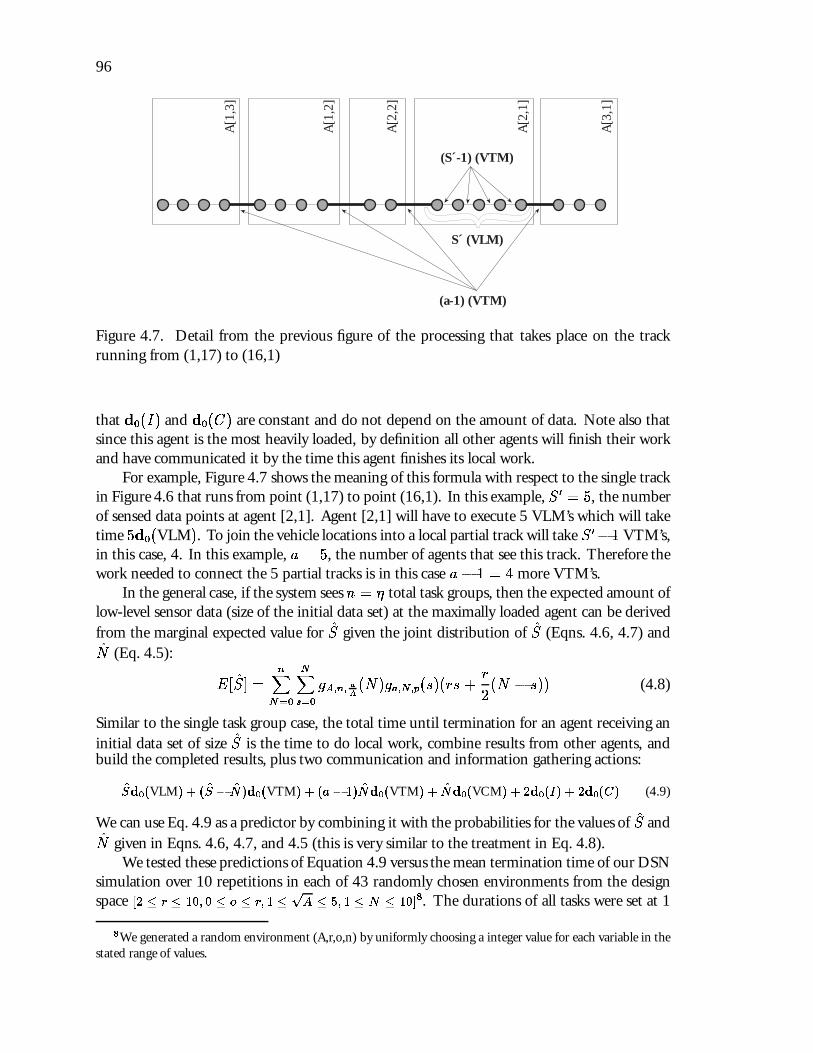
96

A[1

,3]

A[1

,2]

A[2

,2]

A[2

,1]

A[3

,1]

S´ (VLM)

(S´-1) (VTM)

(a-1) (VTM)

Figure 4.7. Detail from the previous figure of the processing that takes place on the trackrunning from (1,17) to (16,1)

that d0(I) and d0(C) are constant and do not depend on the amount of data. Note also thatsince this agent is the most heavily loaded, by definition all other agents will finish their workand have communicated it by the time this agent finishes its local work.

For example, Figure 4.7 shows the meaning of this formula with respect to the single trackin Figure 4.6 that runs from point (1,17) to point (16,1). In this example, S0 = 5, the numberof sensed data points at agent [2,1]. Agent [2,1] will have to execute 5 VLM’s which will taketime 5d0(VLM). To join the vehicle locations into a local partial track will take S0�1 VTM’s,in this case, 4. In this example, a = 5, the number of agents that see this track. Therefore thework needed to connect the 5 partial tracks is in this case a� 1 = 4 more VTM’s.

In the general case, if the system sees n = � total task groups, then the expected amount oflow-level sensor data (size of the initial data set) at the maximally loaded agent can be derivedfrom the marginal expected value for S given the joint distribution of S (Eqns. 4.6, 4.7) andN (Eq. 4.5):

E[S] =nX

N=0

NXs=0

gA;n; aA(N)ga;N;p(s)(rs +

r

2(N � s)) (4.8)

Similar to the single task group case, the total time until termination for an agent receiving aninitial data set of size S is the time to do local work, combine results from other agents, andbuild the completed results, plus two communication and information gathering actions:

Sd0(VLM) + (S � N )d0(VTM) + (a � 1)Nd0(VTM) + Nd0(VCM) + 2d0(I) + 2d0(C) (4.9)

We can use Eq. 4.9 as a predictor by combining it with the probabilities for the values of S andN given in Eqns. 4.6, 4.7, and 4.5 (this is very similar to the treatment in Eq. 4.8).

We tested these predictions of Equation 4.9 versus the mean termination time of our DSNsimulation over 10 repetitions in each of 43 randomly chosen environments from the designspace [2 � r � 10; 0 � o � r; 1 �

pA � 5; 1 � N � 10]8. The durations of all tasks were set at 1

8We generated a random environment (A,r,o,n) by uniformly choosing a integer value for each variable in thestated range of values.

97

time unit, as were the duration of information gathering and communication actions; we willdemonstrate and discuss the effect of this assumption later in the paper. We used the simulationvalidation statistic suggested by Kleijnen [Kleijnen, 1987] (where y = the predicted output bythe analytical model and y = the output of the simulation):

z =y � y

(Var(y) + Var(y))1=2(4.10)

where Var(y) is the predicted variance.9 The result z can then be tested for significance againstthe standard normal tables. In each of the 43 cases, we were unable to reject the null hypothesisthat the actual mean termination equals the predicted mean termination at the � = 0:05 level.For non-statisticians: this is a good thing. The null hypothesis is that our prediction is thesame as the actual value, we did not wish to reject it, and we did not. However, such a test hasproblems since there are other possible reasons which might prevent us from rejecting the nullhypothesis. The best approach to avoiding this problem is to report not only the alpha levelof the test but also the test’s power. With any statistical hypothesis test there are four possibleoutcomes: we are unable to reject the null hypothesis when it is in reality true , we are unableto reject the null hypothesis when it is in reality false (called a Type II error ), we reject thenull hypothesis when it is in reality false, and we reject the null hypothesis when it is in realitytrue (called a Type I error ). The � level is essentially the probability of a Type I error. Thepower of a test is (1 � �), where � is essentially the probability of a Type II error (acceptinga false null hypothesis). Unfortunately, estimating the power of a test is often difficult, andrequires detailed knowledge of the distribution of the test statistic under the condition that thealternative hypothesis is true (this is turn usually requires the computation of the power forseveral likely alternative hypotheses). Future work will involve the computation of the powerfor this statistic, or the development of a new test based on other possible statistics that havebetter-understood power characteristics.

Figure 4.8 shows the mean of 10 repetitions in each environment versus the expected valueand its likelihood intervals. The 50% likelihood interval is included to give you some idea ofthe shape of the underlying distribution; a system designer would of course use the 90% or95% intervals.

The point of this section is that the analytical model describes the implementation fairlywell, and we could use the analytical model to design a good static organization for a givenenvironment, using standard heuristic optimization techniques such as simulated annealing.

4.7.2 Control Costs

The control algorithm presented above is simple and not necessarily optimal. By com-municating only when there is no local work to be done, the heaviest-loaded agent gives upthe chance for other agents to do the high-level composition in a task group by incrementallytransmitting each result (or set of results on a single task group) as it is completed—a maximumpotential savings of (N � 1)(a� 1)d0(VTM) + (N � 1)d0(VCM). However, this needs tobe balanced with the cost of multiple communication actions, which is (N � 1)d0(C). Thus

9The predicted variance of Equation 4.9 can be easily derived from the statistical identity Var(x) = E[x2]�(E[x])2.

98

Run Number

0

20

40

60

80

100

120

1 6 11 16 21 26 31 36 41

90% Likelihood Interval

50% Likelihood Interval

Expected Termination

Actual Mean Termination (10 repetitions)

Term

inat

ion

Tim

e

Figure 4.8. Actual system termination versus analytic expected value and analytically deter-mined 50% and 90% likelihood intervals. Runs arbitrarily ordered by expected terminationtime.

the question of ‘when to communicate’ (when to incrementally transmit partial results) restsdirectly on the cost of communication relative to (a�1)d0(VTM)+d0(VCM) (which dependson both the basic method durations and the agents’ organizational structure). Thus, the moreagents there are that see a single track the more likely it is that intermediate communicationwould be useful.

This simple control algorithm can be analyzed easily, unlike many other systems wherecontrol costs are ignored. If we view the cost of control as the time spent by an agent whennot performing an action (executing a method, information gathering, communication), thenour algorithm runs in constant time between actions except for the two tests [get set of currentlyexecutable methods] and [get set of methods still waiting]. Each of these in the worst case requiresa constant-time test of each element of the full task structure, which is of size O(�r). Thus wesee how the control costs, too, are related to organizational structure.

4.7.3 Analyzing Dynamic Organizations

In the dynamic organizational case, agents are not limited to the original organization andinitial distribution of data. Agents can re-organize by changing the initial static boundaries(changing responsibilities in the overlapping areas), or by shipping raw data to other agents forprocessing (load balancing). We will assume in this section that the agents do not communicateabout the current local state of problem solving directly (see Section 4.8 for thoughts on usingmeta-level communication). A clearer distinction is that in the dynamic organization eachagent makes its initial decision (about changing boundaries or shipping raw data) withoutaccess to non-local information. In the meta-level communication situation the agent wouldhave access to both its local information and a summary of the local state of other agents. In

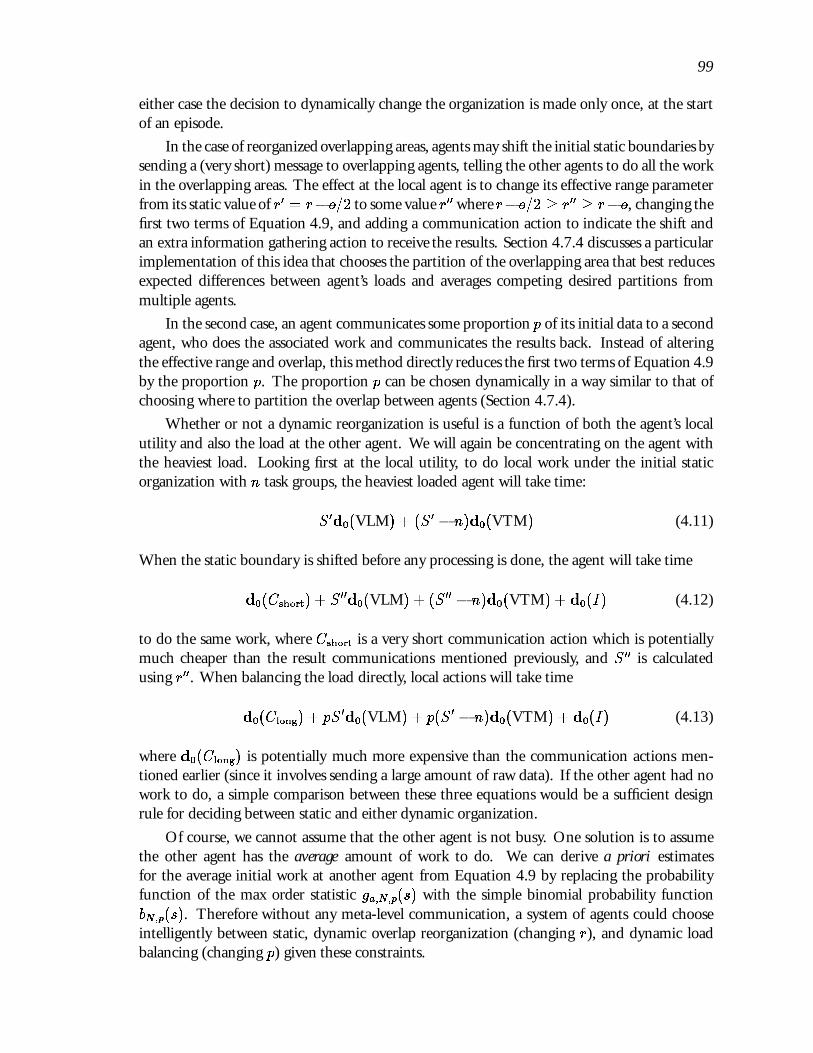
99

either case the decision to dynamically change the organization is made only once, at the startof an episode.

In the case of reorganized overlapping areas, agents may shift the initial static boundaries bysending a (very short) message to overlapping agents, telling the other agents to do all the workin the overlapping areas. The effect at the local agent is to change its effective range parameterfrom its static value of r0 = r�o=2 to some value r00 where r�o=2 � r00 � r�o, changing thefirst two terms of Equation 4.9, and adding a communication action to indicate the shift andan extra information gathering action to receive the results. Section 4.7.4 discusses a particularimplementation of this idea that chooses the partition of the overlapping area that best reducesexpected differences between agent’s loads and averages competing desired partitions frommultiple agents.

In the second case, an agent communicates some proportion p of its initial data to a secondagent, who does the associated work and communicates the results back. Instead of alteringthe effective range and overlap, this method directly reduces the first two terms of Equation 4.9by the proportion p. The proportion p can be chosen dynamically in a way similar to that ofchoosing where to partition the overlap between agents (Section 4.7.4).

Whether or not a dynamic reorganization is useful is a function of both the agent’s localutility and also the load at the other agent. We will again be concentrating on the agent withthe heaviest load. Looking first at the local utility, to do local work under the initial staticorganization with n task groups, the heaviest loaded agent will take time:

S 0d0(VLM) + (S0 � n)d0(VTM) (4.11)

When the static boundary is shifted before any processing is done, the agent will take time

d0(Cshort) + S00d0(VLM) + (S00 � n)d0(VTM) + d0(I) (4.12)

to do the same work, where Cshort is a very short communication action which is potentiallymuch cheaper than the result communications mentioned previously, and S00 is calculatedusing r00. When balancing the load directly, local actions will take time

d0(Clong) + pS0d0(VLM) + p(S0 � n)d0(VTM) + d0(I) (4.13)

where d0(Clong) is potentially much more expensive than the communication actions men-tioned earlier (since it involves sending a large amount of raw data). If the other agent had nowork to do, a simple comparison between these three equations would be a sufficient designrule for deciding between static and either dynamic organization.

Of course, we cannot assume that the other agent is not busy. One solution is to assumethe other agent has the average amount of work to do. We can derive a priori estimatesfor the average initial work at another agent from Equation 4.9 by replacing the probabilityfunction of the max order statistic ga;N;p(s) with the simple binomial probability functionbN;p(s). Therefore without any meta-level communication, a system of agents could chooseintelligently between static, dynamic overlap reorganization (changing r), and dynamic loadbalancing (changing p) given these constraints.

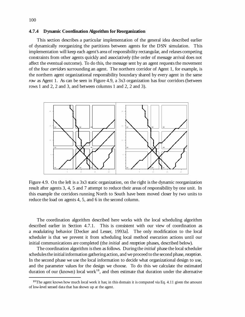
100

4.7.4 Dynamic Coordination Algorithm for Reorganization

This section describes a particular implementation of the general idea described earlierof dynamically reorganizing the partitions between agents for the DSN simulation. Thisimplementation will keep each agent’s area of responsibility rectangular, and relaxes competingconstraints from other agents quickly and associatively (the order of message arrival does notaffect the eventual outcome). To do this, the message sent by an agent requests the movementof the four corridors surrounding an agent. The northern corridor of Agent 1, for example, isthe northern agent organizational responsibility boundary shared by every agent in the samerow as Agent 1. As can be seen in Figure 4.9, a 3x3 organization has four corridors (betweenrows 1 and 2, 2 and 3, and between columns 1 and 2, 2 and 3).

A1

A2

A3

A4

A5

A6

A7

A8

A9

5

10

20

15

5 10 2015

A1

A2

A3

A4

A5

A6

A7

A8

A9

5

10

20

15

5 10 2015

Figure 4.9. On the left is a 3x3 static organization, on the right is the dynamic reorganizationresult after agents 3, 4, 5 and 7 attempt to reduce their areas of responsibility by one unit. Inthis example the corridors running North to South have been moved closer by two units toreduce the load on agents 4, 5, and 6 in the second column.

The coordination algorithm described here works with the local scheduling algorithmdescribed earlier in Section 4.7.1. This is consistent with our view of coordination asa modulating behavior [Decker and Lesser, 1993a]. The only modification to the localscheduler is that we prevent it from scheduling local method execution actions until ourinitial communications are completed (the initial and reception phases, described below).

The coordination algorithm is then as follows. During the initial phase the local schedulerschedules the initial information gathering action, and we proceed to the second phase, reception.In the second phase we use the local information to decide what organizational design to use,and the parameter values for the design we choose. To do this we calculate the estimatedduration of our (known) local work10, and then estimate that duration under the alternative

10The agent knows how much local work it has; in this domain it is computed via Eq. 4.11 given the amountof low-level sensed data that has shown up at the agent.

101

organizations (dynamic reorganization or load-balancing). When a parameter needs to beestimated, we do so to minimize the absolute expected difference between the amount of workto be done locally and the amount of work done at the remote agent that is impacted the mostby the proposed change.

For example, when dynamically restructuring, if the overlap between agents is more than2 units, we have a choice of reducing the area an agent is responsible for by more than 1 unit(this is the organizational design parameter � in question). To decide on the proper reduction(if any), each agent computes its known local work W (�) using Eq. 4.11 with the actual (notestimated) S0 and N computed assuming the agent’s area is reduced by �. Then the agent findsthe value of � that minimizes the difference in its known local work W (r� �) and the averagework �W (r + �) at the other agent:

S(r; s;N) = (rs+r

2(N � s))

W (r; s;N) = S(r; s;N)d0(VLM) + (S(r; s;N)�N)d0(VTM)

E[W (r)] =nX

N=0

NXs=0

gA;n; aA(N)ga;N;p(s)W (r; s;N) (4.14)

E[ �W (r)] =nX

N=0

NXs=0

bn; aA(N)bN;p(s)W (r; s;N) (4.15)

Equation 4.15 is just a restatement of Eqn. 4.14 (itself derived from Eqns. 4.5, 4.6, 4.7,and 4.11 for the case of the average, not maximally loaded, agent (thus the use of b, thebinomial probability function rather than g, the max order statistic p.f.)).

If � = 0, then the agent will not restructure. If � 6= 0, then the agent sends a message toall affected agents requesting a reduction of amount � in each corridor (north, east, south, andwest). The agent sets its current area of interest to include only the unique (non-overlapping)portion of its area (if any), and enters the unique-processing phase. During this phase the regularlocal scheduler described earlier controls method execution actions.

When no more methods unique to this agent can be executed, the coordination algorithmchecks the current time. If enough time has passed for the messages from other agents (if any)to arrive (this depends on the communication delays in the system), the coordination algorithmschedules an information-gathering action to retrieve the messages. Note that every agent mayreach this point at a different time; agents with a large amount of unique local work may takesome time, agents with no work at all will wait idle for the length of communication delay timein the system.

At this point each agent will relax its borders according to the wishes of the other agents.The relaxation algorithm we have chosen is fairly simple and straightforward, though severalsimilar choices are possible. The algorithm is symmetric with respect to the four corridorssurrounding the agent, so we will just discuss the relaxation of the northern corridor. Therewill be a set of messages about that corridor, some wanting it moved up by some amount andsome wanting it moved down by some amount—we will consider these as positive and negativevotes of some magnitude. The relaxation algorithm sums the votes, and returns the sum unlessit is larger than the maximum vote or smaller than the minimum vote, in which case the max or

102

min is returned, respectively.11 At this point the agent enters the final normal processing phase,and the local scheduler schedules all further actions as described earlier.

4.7.5 Analyzing the Dynamic Restructuring Algorithm

As we did in Section 4.7.1, we can develop an expression for the termination time of anyepisode where the agents follow this algorithm. To do so, we start with the basic terminationtime given all of the random variables. This equation is derived from Eqns. 4.14 and 4.15:

T (r; S; N ; �s; �N ) = max[W (r � �; S; N );W (r + �; �s; �N)] (4.16)

where � is computed as described in the last section using the given values of (r; S; N; �s; �N ). Toturn this into a predictive formula, we then use the expressions for the probabilities of the termsS; N ; �s; and �N (from Eqns. 4.6, 4.7, and 4.5). For example, we can produce an expression forthe expected termination of the algorithm:

nXN=0

NXS=0

nX�N=0

�NX�s=0

gA;n; aA(N)ga;N;0:5(s)bn; aA (

�N)b �N;0:5(�s)T (r; S; N; �s; �N) (4.17)

We tested the predictions of Equation 4.17 versus the mean termination time of ourDSN simulation over 10 repetitions in each of 10 randomly chosen environments. Thedurations of all tasks were set at 1 time unit, as were the duration of information gathering andcommunication actions, with the exception of the 4 environments described in the next section.Using the same validation statistic as before (Eq. 4.10) in each case we were unable to rejectthe null hypothesis that the actual mean termination equals the predicted mean termination atthe � = 0:05 level.12

4.7.5.1 Increasing Task Durations

Figures 4.10 through 4.13 compare the termination of static and dynamic restructuringorganizations on identical episodes in four different environments. Ten different episodeswere generated for each environment. In order to see the benefits of dynamic restructuringmore clearly, we chose task durations for each environment similar to those in the DVMT:d0(VLM) = 6;d0(VTM) = 2d0(VCM) = 2.13 Note that the dynamic organization oftendoes significantly better than the static organization, and rarely does much worse—rememberthat is many particular episodes that the dynamically organized agents will decide to keepthe static organization, although they pay a constant overhead when they keep the staticorganization (one extra communication action and one extra information gathering action,given that the time for a message to reach all agents is no longer than the communicationaction time).

11For example, if 2 agents vote for it to be moved up by one, and two vote for it to be moved up by 2, then thecorridor is moved up by only 2, not 6!

12The same caveats that we discussed in Section 4.7.1 still apply here.13The idea being that the VLM methods correspond to lowest three DVMT KSIs as a group, and the other

methods correspond to single DVMT KSIs, and that a KSI has twice the duration of a communication action.

103

E

E

E

E E

E

E

E

E

E

G

G

G

G

G

G

G

G

G

G

0

50

100

150

200

250

Ter

min

atio

n T

ime

Dynamic termination timeStatic termination timeG

E

Figure 4.10. Paired-response comparison of the termination of static and dynamic systems theenvironment A = 9; r = 9; o = 9; n = 7] (ten episodes). Task durations are set to simulatethe DVMT (see text).

EE

EE E

E EE

E

E

G

G

G

G G G

G

G

G

G

0

20

40

60

80

100

120

140

Ter

min

atio

n T

ime

Dynamic termination timeStatic termination timeG

E

Figure 4.11. Paired-response comparison of the termination of static and dynamic systems theenvironment A = 16; r = 8; o = 5; n = 4] (ten episodes). Task durations are set to simulatethe DVMT (see text).

104

E

E

E

E

EE

E

EE

E

G

G

G

G

G

G

G

GG

G

0

50

100

150

200

250

300

Ter

min

atio

n T

ime

Dynamic termination timeStatic termination timeG

E

Figure 4.12. Paired-response comparison of the termination of static and dynamic systems theenvironment A = 4; r = 9; o = 3; n = 5] (ten episodes). Task durations are set to simulatethe DVMT (see text).

E

E

EE

E

E

E E

E

E

G

G

GG

G

G

G

G

G

G

0

50

100

150

200

250

300

350

Ter

min

atio

n T

ime

Dynamic termination timeStatic termination timeG

E

Figure 4.13. Paired-response comparison of the termination of static and dynamic systems theenvironment A = 9; r = 10; o = 6; n = 7] (ten episodes). Task durations are set to simulatethe DVMT (see text).

105

4.8 Using Meta-Level Communication

For some environments D =< A; �; r; o;T > one of the three organizational choices(static, reorganized, load balanced) may be clearly better in the long run, but for mostenvironments the choice is not so clear given the variance in system performance. Thechoice that optimizes performance over the long run is often not optimal in any particularepisode. Taking the essential equations for local work in Section 4.7.3, we can computelikelihood intervals on the predicted performance of an organization under each of the threecoordination regimes by combining the local likelihood interval on the expected load of theheaviest loaded agent, and the likelihood interval on the average agent load. These results,for the 90% likelihood interval, are shown in Figures 4.14 through 4.19. Again we haveassumed that all execution, communication, and information gathering action durations havethe same value (making communication relatively expensive). The first figures, Figures 4.14through 4.16, highlight how the relationship between performance under a static organizationand a dynamically load balanced organization changes as the number of agents increases. Asexpected, load balancing becomes more desirable as the number of agents increases (in relationto the average number of tracks): when there are many agents, the average agent load becomesvery low, which offsets the cost of transferring tasks. In this figure the performance differencebetween static and overlap reorganization remains nearly constant relative to the number ofagents.

Figures 4.17 through 4.19 point out how dynamically reorganizing the overlap areaincreases the performance over static organization as the amount of overlap increases. Thisresult is consistent with Durfee’s results [Durfee et al., 1987]. For this graph we assumedthat the agents would shrink their entire area of responsibility (as opposed to minimizing thedifference in maximum versus average work as described in Section 4.7.4) to try to maximizethe visual difference on the graph. This graph shows the need for dynamically calculating thereorganized algorithm shrinkage parameter (�) especially at high levels of overlap (note howthe dynamically reorganized organization is predicted to do worse at high levels of overlap(o = 8; 9; 10) in the n = 20 portion). The expected performance difference between the staticorganization and load balancing remains relatively constant across changing values of o. Inboth figures we have let d0(C) = d0(Cshort) = d0(Clong); increasing the differences in thesevalues will move the corresponding curves directly up or down.

The next series of figures demonstrate the effect of the ratio of computation duration tocommunication duration. This and subsequent figures assume that the dynamic restructuringshrinkage parameter � is set to minimize the difference between maximum and average localwork as described in Section 4.7.4. Figure 4.20 shows how the expected value and 90%likelihood interval on system termination changes as the duration of a method execution actionchanges from equal to (1x) a communication action to 10 times (10x) that of a communicationaction. The task structure remains than of the DSN example described in Section 4.5. InFigure 4.20 we see a clear separation emerge between static and dynamic termination. We didnot experiment with changing the communications delay between agents (which is fixed hereat 1 time unit) because all data for an episode arrives at once. In continuous environmentsdelay will be more important (see Section 6.1.5 and [Mirchandaney et al., 1989])

These figures assume that the number of task groups n is known beforehand. The reasonfor this is to highlight the variance implicit in the organization, and minimize the influence ofthe external environment. Figure 4.21 shows how much extra variance is added when only the

106

H H H

H H H H H

H

P

P P P

P P P P P

K

K

K

K K K

K K

K

K

K K K

K K K K K

n

n

n

n n n n n

n

o

o o o

o o o o o

4 9 16 25 36 49 64 81 1000

10

20

30

40

50

60

70

80

90

100

Ter

min

atio

n T

ime

Number of Agents [r=10, o=3, n=5]

Static

Load Balanced

Reorganized

Q R

L L

[ ]

Figure 4.14. 90% likelihood intervals on the expected termination of a system under threecoordination regimes, different numbers of agents, and n = 5.

107

H

H

H H

H

H

H H H

P P

P P P P

P P P

K

K

K K

KK

K K

K

K

K

K K K KK K K

n

n

n n

n

n

n n n

o o

o o o o

o o o

4 9 16 25 36 49 64 81 1000

20

40

60

80

100

120

140

160

Ter

min

atio

n T

ime

Number of Agents [r=10, o=3, n=10]

Static

Load Balanced

Reorganized

Q R

L L

[ ]

Figure 4.15. 90% likelihood intervals on the expected termination of a system under threecoordination regimes, different numbers of agents, and n = 10.

108

H

H

H

H H

H

H H H

P

P

P

P P P

P P

P

K

K

K

KK

K KK K

K

K

K

KK K

K KK

n

n

n

n nn

n n no

oo

o o oo o

o

4 9 16 25 36 49 64 81 1000

50

100

150

200

250

300

Ter

min

atio

n T

ime

Number of Agents [r=10, o=3, n=20]

Static

Load Balanced

Reorganized

Q R

L L

[ ]

Figure 4.16. 90% likelihood intervals on the expected termination of a system under threecoordination regimes, different numbers of agents, and n = 20.

109

H

H

H

H

H

H

H

H

H

H

H

P P

P

P

P P

P

P

P P

P

K

K

K

K K K K K K K K

KK

KK

KK

KK

KK

K

0 1 2 3 4 5 6 7 8 9 100

10

20

30

40

50

60

70

80

90

Ter

min

atio

n T

ime

Overlap [A=9, r=10, n=5]

Static

Reorganized

Q R

L L

Figure 4.17. 90% likelihood intervals on the expected termination of a system under twocontrol regimes, varying the amount of overlap, with n = 5.

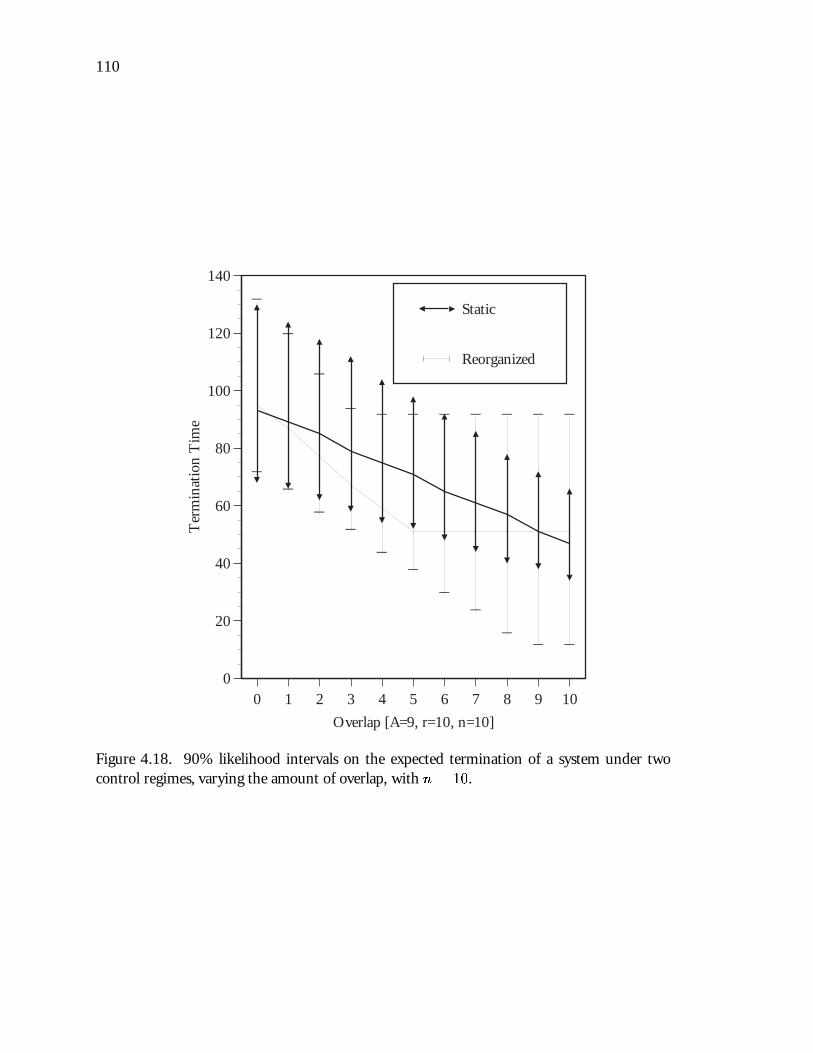
110

H

H

H

H

H

H

H

H

H

H

H

PP

P

P

PP

P

P

PP

P

K

K

K

KK K K K K K K

K

K

K

K

K

K

K

K

KK K

0 1 2 3 4 5 6 7 8 9 100

20

40

60

80

100

120

140

Ter

min

atio

n T

ime

Overlap [A=9, r=10, n=10]

Static

Reorganized

Q R

L L

Figure 4.18. 90% likelihood intervals on the expected termination of a system under twocontrol regimes, varying the amount of overlap, with n = 10.

111

H

H

H

H

H

H

H

H

H

H

H

P

P

P

P

P

P

P

P

P

P

P

K

K

K K K K K K K K K

K

K

K

K

K

K

K K K K K

0 1 2 3 4 5 6 7 8 9 100

50

100

150

200

250

Ter

min

atio

n T

ime

Overlap [A=9, r=10, n=20]

Static

Reorganized

Q R

L L

Figure 4.19. 90% likelihood intervals on the expected termination of a system under twocontrol regimes, varying the amount of overlap, with n = 20.

112

K

K

K

K

K

K

K

K

K

K

KK

KK

KK

KK

KK

X

X

X

X

X

X

X

X

X

X

K

K

K

K

K

K

K

K

K

K

KK

KK

KK

KK

KK

XX

XX

XX

XX

XX

1x 2x 3x 4x 5x 6x 7x 8x 9x 10x0

100

200

300

400

500

600

700E

stim

ated

Ter

min

atio

n

Cost of execution vs. communication

X Static Organization

X Dynamic Restructuring

Figure 4.20. Effect of decreasing communication costs on expected termination under astatic organization and dynamic restructuring (expected value and 90% likelihood interval,A = 25; r = 9; o = 9; n = 7).

expected value of n, which is �, is known. We assume that the number of task groups n (in theDSN example, vehicle tracks) that occur during a particular episode has a Poisson distributionwith an expected value of �. The discrete probability function for the Poisson distribution,given in any statistics book, is then:

p�(y) = �y

y! e�y [Pr [n = y]]

We can use this probability in conjunction with Eqns. 4.8, 4.11, and 4.15 to calculate theexpected value, 50%, and 95% likelihood intervals on termination in the static or dynamicorganizations.14 Note in Figure 4.21 both the large increase in variance when n is random(between the top bar and the third bar in the figure), and more importantly the small decreasein variance in the dynamic restructuring organization (between the first and the second bars).Note also that the mean termination time for the dynamic organization is slightly less than thatfor the static organization.

These figures bring us to the final point of this chapter: often system performance canbe improved significantly by dynamic reorganization, but it will rarely always be improved.On average the dynamic algorithm does better, especially when computation is more expensivethan communication, and assuming that there is some overlapping sensor area with whichto trade off computation. Meta-level communication between agents about their local loadsshould, with a small communication cost, pinpoint the true costs and benefits of the variousorganizational structures, allowing an informed organizational decision to be made. Instead ofan agent making a decision about restructuring or load balancing by assuming the average load,

14Again, we are providing the 50% interval just to allow the reader to imagine the shape of the underlyingdistribution better.

113

Mean

50% Likelihood Interval

95% Likelihood Interval

Estimated Termination Time

35 85 135 185

Dynamic, n known

Static, n known

Dynamic, n Poisson

Static, n Poisson

Var = 520

Var = 608

Var = 1450

Var = 1780

Figure 4.21. Demonstration of both the large increase in performance variance when thenumber of task groups n is a random variable, and the small decrease in variance with dynamicrestructuring coordination [A = 9; r = 9; o = 9]. Where n is known, n = 7. Where n is arandom variable, the expected value � = 7.

the agent will have the actual load for the neighboring agents. As we said in the introduction,the proper organization is often one that exploits information that resolves uncertainties aboutthe current environment as it becomes available to the agents, allowing the agents to then createthe most efficient organization for the situation.

4.9 Summary

What have I shown in this chapter? I have shown that TÆMS can be used to build modelsof task environments that can be analyzed mathematically, and in conjunction with simplealgorithms for coordinated behavior. In this chapter I showed how variations in terminationtime could be explained and predicted by environmental variation and the agent’s coordinationalgorithm, a much more satisfying answer than the weaker ‘no one algorithm was always thebest’ given in earlier work [Durfee et al., 1987].

This chapter also demonstrated a methodology for the analysis and design of coordinationand scheduling mechanisms, based on MAD. The first step was to build a model of theenvironment of interest, using TÆMS, in Sections 4.1 through 4.6. At this point the analysis ofthe endogenous features (such as S and N ) of individual episodes, given generative parameters,also took place.

The astute reader will notice that in fact detailed TÆMS structures come in to play for onlypart of the analysis done here. It is important to point out that even when TÆMS does notgive specific tools (like a task structure) for modeling, it still provides a structured method bywhich modeling can proceed. Thus even though TÆMS does not yet provide us with canned

114

representations for generative models, it does provide us with, for example, the output of thegenerative model (some task structure or set of task structures). In this way TÆMS helped usgreatly to focus on exactly what should go into the generative model and what was extraneous15.

TÆMS assumes only a simple view of agents as loci of belief (state) and action. Themathematical analysis in this chapter proceeded with a formal specification of what actionsan agent will take based on its current beliefs, using the TÆMS-provided meta-structure forthe agent’s state-transition function (control, information gathering, communication, andmethod execution). This chapter looked at two combined control-and-coordination algorithmsfor agent action (the static algorithm in Section 4.7.1, the one-shot dynamic algorithm inSection 4.7.4 and the meta-level control algorithm in Section 4.7.3).

This chapter then showed the use of the methodology to develop expressions for theexpected value of, and likelihood intervals on, the time of termination of a set of agents in anyarbitrary simple DSN environment that has a static organizational structure and coordinationalgorithm. For example, the total time until termination for an agent receiving an initial dataset of size S is the time to do local work, combine results from other agents, and build thecompleted results, plus two communication and information gathering actions:

Sd0(VLM) + (S � N )d0(VTM) + (a� 1)Nd0(VTM) + Nd0(VCM) + 2d0(I) + 2d0(C) (4.18)

Eq. 4.9 can be used as a predictor by combining it with the probabilities for the values of Sand N . I verified this model using the simulation component of TÆMS.

Using this model as a starting point, I extended it to analyze a dynamic, one-shotreorganization algorithm (and have shown when the extra overhead is worthwhile versusthe static algorithm). In each case I can predict the effects of adding more agents (Figures4.14–4.16), changing the relative cost of communication and computation (Figure 4.20), andchanging how the agents are organized (in this case, by changing the range and overlap oftheir capabilities, Figures 4.17–fig:von20). These results were achieved by direct mathematicalanalysis of the model and verified through simulation in TÆMS. This represents a significantstep forward in work on modeling DAI systems.

I specialize MAD by generative model of environmental variance (such as the number oftracks or the load at the most heavily loaded agent). I also demonstrated the importance ofenvironmental variance with respect to agent load balancing and meta-level communication inSection 4.7.5 (I’ll return to this question in Section 6.6).

The TÆMS framework for describing complex task environments is intentionally designedto bring together experimental work on complex environments and formal work on theprincipled construction of agents that act rationally and predictably based on their beliefs,desires, intentions, and goals. I have shown this by applying formal methods to a DSNtask with coordination opportunities that are much more complex than single-instance gamematrices. The simulation component, which requires the implementation of the ideas, notjust abstract analysis, rounds out the picture. At the very least, I hope this approach will allowideas to be more carefully expressed and thus more approachable by the AI community. Iwill continue this demonstration in the next chapter through the development and the use ofcommitments.

In this chapter, stylized information gathering actions are used to represent actions such as‘running external sensors’. The inclusion of explicit information gathering actions, is unique

15See also the discussion in Section 3.6.1.

115

and useful for building models at the ‘appropriate’ level relative to the question being asked.They are a powerful abstraction mechanism that can replace complex reasoning processes (e.g.,planning) with simpler time/computation tradeoffs for the purpose of modeling. Often a large,complex system will have many components, not all of which will be under study, or designed.Information gathering actions are used to represent the gross behaviors of these components andanticipate system interactions (or explore possible interactions through perturbation) beforeand during their design.

Currently there are no characterizations for non-formal coordination algorithms, or forformal techniques in complex environments. This chapter described such a characterization,as will the next.

In the next two chapters, I will move from the simple coordination mechanisms used inthese chapters to a family of coordination algorithms constructed from an expandable set ofsimpler coordination mechanisms. Because these algorithms are more complex and dynamic, Iwill also move from static, closed-form analyses to simulation-based analyses (but these will usewell-characterized environment specifications and many properly generated test episodes—nota few, hand-picked examples).

116

C H A P T E R 5

GENERALIZED PARTIAL GLOBAL PLANNING

That is, the relations among what we call our ‘actions’, ‘knowledge’, ‘beliefs’, ‘goals’,and ‘interests’ consist of continuous interactions among various structures, mechanisms,traces, impulses, and tendencies that are not necessarily (‘naturally’ or otherwise) consis-tent, coordinated, or synchronized and are therefore always more or less inconsistent,out-of-phase, discordant, and conflictual.

— Barbara Hernstein Smith, Contingencies of Value: Alternative Perspectives forCritical Theory, 1988

Many researchers have shown that there is no single best organization or coordinationmechanism for all environments. This and the following chapters discuss the design andimplementation of an extendable family of coordination mechanisms, called Generalized PartialGlobal Planning (GPGP), that form a basic set of coordination mechanisms for teams ofcooperative computational agents. The important features of this approach include a set ofmodular coordination components called “mechanisms” (any subset or all of which can beused in response to a particular task environment); a general specification of these mechanismsinvolving the detection and response to certain abstract coordination relationships in theincoming task structure that are not tied to a particular domain; and a separation of thecoordination mechanisms from an agent’s local scheduler that allows each to better do the jobfor which it was designed. Each component or mechanism can be added as required in reactionto the environment in which the agents find themselves a part. An individual algorithm inthe family is defined by a particular set of active mechanisms and their associated parameters.In Chapter 6 I will also discuss the interactions between these mechanisms and how to decidewhen each mechanism should be used, drawing data from simulation experiments of multipleagent teams working in abstract task environments.

The GPGP approach specifies three basic areas of the agent’s coordination behavior: howand when to communicate and construct non-local views of the current problem solvingsituation; how and when to exchange the partial results of problem solving; how and whento make and break commitments to other agents about what results will be available andwhen. The GPGP approach of recognizing and reacting to the characteristics of certaincoordination relationships is shared with Von Martial’s work on the favor relationship [v.Martial, 1992]. The use of commitments in the GPGP family of algorithms is based on the ideasof many other researchers [Cohen and Levesque, 1990, Shoham, 1991, Castelfranchi, 1993,Jennings, 1993]. Each agent also has a heuristic local scheduler that decides what actionsthe agent should take and when, based on its current view of the problem solving situation(including the commitments it has made), and a utility function. The coordination mechanismssupply non-local views of problem solving to the local scheduler, including what non-local

118

results will be available locally, and when they will be available. The local scheduler createsand monitors the execution of schedules that attempt to maximize group quality through bothlocal action and the use of non-local actions (committed to by other agents).

One way to think about this work, as I discussed in the overview (Chapter 1), is that theGPGP approach views coordination as modulating local control, not supplanting it—a two levelprocess that makes a clear distinction between coordination behavior and local scheduling. Thisprocess occurs via a set of coordination mechanisms that post constraints to the local schedulerabout the importance of certain tasks and appropriate times for their initiation and completion.By concentrating on the creation of local scheduling constraints, we avoid the sequentiality ofscheduling in the original PGP algorithm [Durfee and Lesser, 1991] that occurs when thereare multiple plans. By having separate modules for coordination and local scheduling, wecan also take advantage of advances in real-time scheduling algorithms to produce cooperativedistributed problem solving systems that respond to real-time deadlines. We can also takeadvantage of local schedulers that have a great deal of domain scheduling knowledge alreadyencoded within them. Finally, our approach allows consideration of termination issues thatwere glossed over in the PGP work (where termination was handled by an external oracle). Idiscuss how to decide when each mechanism should be used and how the mechanisms interact,drawing on simple models of generic task structures and data from simulation experimentswhere multiple agent teams work in abstract task environments, in the next chapter (Chapter 6).

The way that we specify the family of algorithms in a general, domain-independent way(as responses to certain environmental situations and interactions with a local scheduler) isvery important. It leads to the eventual construction of libraries of reusable coordinationcomponents that can be chosen (customized) with respect to certain attributes of the targetapplication.

As an example of how different coordination mechanisms can dramatically effect per-formance in identical environments, consider Crowston’s observation of restaurant service atthe TGI Fridays chain [Crowston, 1994]. The task structure and process at any two TGIFridays restaurants are essentially identical (it is a sit-down restaurant). Crowston discusses twodifferent Fridays locations of equal size. However, the wait time to be seated during periods ofheavy use (i.e. the lunch and dinner rush) at the newer of the two locations is reduced to anaverage of 15 minutes from an hour. The difference between the restaurants is not the structureof their tasks, but the coordination mechanisms. In the old location, enablement relationshipsbetween tasks—the table must be bussed before customers can be seated, the food must becooked and assembled before it can be served—are coordinated by polling on the consumer sideof the relationship (the host scans for free tables, the waitstaff checks at the kitchen for a table’sfood order to be up). In the newer, faster restaurant the consumer of an enables relationshipis notified (a computer screen at the host’s station shows free tables and is updated remotelyby the cleaning staff as soon as a table is bussed; waitstaff is paged by the kitchen when anorder is complete, etc.). Changing the coordination mechanisms has dramatically improvedperformance during peak times for this organization.

The first section in this chapter will describe the details of the original PGP algorithmthat were not covered in Chapter 2, and discuss how we will extend it. The next section willdeal in a general way with decisions faced by agents that are coordinating their behavior over acoordination relationship such as facilitates. Section 5.2 will introduce the Generalized PartialGlobal Planning (GPGP) approach. Sections 5.4 through 5.6 will describe our assumptions

119

about the agents’ architecture. Briefly, we assume each agent has a local scheduler whichschedules local actions in an attempt to maximize some utility measure defined on a TÆMS taskstructure. We also assume that the local scheduler at each agent understands two special typesof constraints, called local and non-local commitments, that we will describe in this chapter.We also assume that each agent has a GPGP coordination module and a set of coordinationmechanisms. We will describe how the coordination module and the local scheduler interact.Finally, Section 5.7 describes the interface between the local scheduler and the coordinationmodule in more detail.

5.1 Partial Global Planning

Partial global planning [Durfee and Lesser, 1991] was developed as a distributed controltechnique to insure coherent network problem solving behavior. It is a flexible approach tocoordination that does not assume any particular distribution of subproblems, expertise, orother resources, but instead lets nodes coordinate in response to the current situation. Eachnode can represent and reason about the actions and interactions of groups of nodes and howthey affect local activities. These representations are called partial global plans (PGPs) becausethey specify how different parts of the network plan to achieve more global goals. Each node canmaintain its own set of PGPs that it may use independently and asynchronously to coordinateits activities.

A PGP contains an objective, a plan-activity-map, a solution-construction-graph and astatus[Durfee and Lesser, 1991]:

� The objective contains information about why the PGP exists, including its eventualgoal (the larger solution being formed) and its importance (a priority rating or reasonsfor pursuing it).

� The plan-activity-map represents what the nodes are doing, including the major plansteps the nodes are concurrently taking, their costs, and expected results.

� The solution-construction-graph contains information about how the nodes shouldinteract, including specifications about what partial results to exchange and when toexchange them.

� The status contains bookkeeping information for the PGP, including pointers to relevantinformation received from other nodes and when that information was received.

A PGP is a general structure for representing coordinated activity in terms of goals, actions,interactions and relationships.

When in operation, a node’s PGPlanner scans its current network model (a node’srepresentation of the goals, actions and plans of other nodes in the system) to identify whenseveral nodes are working on goals that are pieces of some larger network goal (partial globalgoal). By combining information from its own plans and those of other nodes, a PGPlannerbuilds PGPs to achieve the partial global goals. A PGPlanner forms a plan-activity-map fromthe separate plans by interleaving the plans’ major steps using the predictions about whenthose steps will take place. Thus, the plan-activity-map represents concurrent node activities.To improve coordination, a PGPlanner reorders the activities in the plan-activity-map usingexpectations or predictions about their costs, results, and utilities. Rather than examining all

120

possible orderings, a PGPlanner uses a hill-climbing procedure to cheaply find a better (thoughnot always optimal) ordering. From the reordered plan-activity-map, a PGPlanner modifiesthe local plans to pursue their major plan steps in a more coordinated fashion. A PGPlanneralso builds a solution-construction-graph that represents the interactions between nodes. Byexamining the plan-activity-map, a PGPlanner identifies when and where partial results shouldbe exchanged in order for the nodes to integrate them into a complete solution, and thisinformation is represented in the solution-construction-graph.

Why does partial global planning work well in the DVMT? It is because:

� It avoids redundant work among nodes by noticing interactions among the differentlocal plans. Specifically, it notices when two node plans have identical intermediategoals, i.e., when they are generating interpretations of the same region in time and space.This occurs in the DVMT because, in the interest of reliability, nodes have overlappingsensors.

� It schedules the generation of partial results so that they are transmitted to other nodesand assist them at the correct time. To do this it uses the estimates of the times thatactivities will take and the inferred relation that if node A estimates that it will take lesstime than node B to complete an intermediate goal, and the goals are spatially near, thatnode A can provide facilitative information to node B.

� It allocates excess tasks from overloaded nodes to idle nodes. Node plans provide theinformation needed to determine if a node is overburdened or underutilized. A nodeis underutilized if it is either idle or participates in only low-rated PGPs. A node isoverburdened if its estimated completion time of a subgoal of goal G is much later thanthe completion time of all the other subgoals of G [Durfee and Lesser, 1989].

� It assumes that a goal is more likely to be correct if it is compatible with goals at othernodes. In the DVMT task, a goal represented a processing task to ascertain whether avehicle was moving in a region r at time t. This goal could, in fact, be wrong—basedon noise or errorful sensor data that was the basis for the preliminary task analysis thatgenerated the goal. Nodes choose local plans to work on based on the highly rated PGPsthey have received. Thus, if the intermediate goals of a node become part of a PGP, thenthey are worked on before other intermediate goals in other local plans the node mayhave (even though the node may have rated those local plans higher in its local view).

� It is terminated externally when it first reaches the correct solution, rather than throughsome internal termination criteria.

The partial global planning framework lets nodes converge on common PGPs in a stableenvironment (where plans do not change because of new data, failed actions, or unexpectedeffects of their actions). When network, data, and problem-solving characteristics change andcommunication channels have delay and limited capacity, nodes can locally respond to newsituations, still cooperating but with potentially less effectiveness because they have somewhatinconsistent PGPs [Durfee and Lesser, 1988a]. The PGP framework does not deal withconflicts in physical resources.

The original PGP algorithm orders intermediate ‘goals’ according to their cost as computedfrom the cross-product of a vector of seven computable factors (described below) and globalcooperation parameters that give a weight to the corresponding term in the calculation. In

121

our approach, this information has been captured symbolically by the task structure. ThePGP ‘goals’ were communicated at a fixed level of detail, and corresponded directly to tasks oractivities. We could re-implement most of the original PGP algorithm by using a hill-climbinglocal scheduler, and assigning a priority according to the original PGP evaluation function—however, we are instead using a more sophisticated local scheduler that can understand morecomplex constraints such as delays and deadlines. The Durfee PGP hill climbing schedulerworked by computing a ‘cost’ for each activity/goal in the plan, and trying to order the planso that the least expensive activities were earlier. There were seven factors that went intocomputing the cost for each plan activity. The relationship of each of the seven factors used inthe original PGP evaluation function to our new representations is as follows [Note that theseterms are the terms used in Durfee’s thesis, and differ considerably from the usage of theseterms in work on distributed operating systems]:

PGP Redundancy: Was defined by Durfee as the number of nodes that can perform thisgoal/activity/task. Thus, a plan activity with a high ‘redundancy’ score would be movedlater in the plan. A GPGP local scheduler can use the equality and subtask relationshipsin the TÆMS task structure to determine redundancy.

PGP Reliability: Was defined by Durfee as the number of nodes that cannot perform this goal.This is the inverse of Durfee’s definition of PGP redundancy.

PGP Duration: Was defined by Durfee as the duration of the goal/activity/task. Obviously aGPGP local scheduler can obtain this measure from a TÆMS task structure as well.

PGP Predictiveness: Durfee defined this as follows. Any goal with a duration of x couldprovide predictive information for a goal of duration y if x < y. The predictivenessmeasure was then the minimum activity distance (minimum number of sensed times)between the two goals. Obviously this definition is only useful for the DVMT. GPGPgeneralizes this concept to the facilitates relationship or similar relationships and considersit to be a domain-dependent relationship.

PGP Locally-predicted: Was defined by Durfee as the minimum activity distance (minimumnumber of sensed times) between a goal and any goal to be executed before it. The effectof this measure was to keep a node from jumping around between times in constructinga track; extending an existing partial solution was preferred. A GPGP local schedulerhas available the subtask-oriented, hierarchical construction of the task structure. GPGPdoesn’t require absolute stability in the local schedule as long as the commitments madeto other agents are met.

Independence: Was defined by Durfee as how many goals occurred before a given goal in theinitial local node plan. This measure was intended to keep the PGPlanner from strayingtoo far from the original local node plan ordering—goals that were originally late inthe ordering would tend to stay late in the PGP ordering. The independence measurefor each goal is constant, because it depends only on the initial local node plan, not onthe position of the goal in the re-ordered plan. Goals later in the initial ordering havehigher independence measures. Because the PGP algorithm used a swapping procedureto create a new ordering from the old, the higher independence measure made later goalsharder to swap. A GPGP local scheduler receives local ordering preferences, and so itknows what local orderings were necessary, which may be negotiated, and which are only

122

preferences. Because the local scheduler is not supplanted by a separate PGPlanningscheduler, this relationship is not directly needed.

Diversity: Durfee defined the diversity value of a goal as 0 if it did not derive redundant infor-mation, and also 0 if all goals following it derived redundant information. Otherwise, thediversity of a goal was measured by the minimum activity distance between the goal andthe later non-redundant goals. The effect was to plan to do non-redundant work beforeredundant work. The GPGP coordination mechanisms detect redundancy throughcoordination relationships instead, so this DVMT-specific measure is not needed.

5.1.1 Issues in Extending the PGP Mechanisms

5.1.1.1 Heterogeneous Agents

How can the PGP mechanisms be extended to handle agents that have different localproblem solving criteria? This can arise in several ways:

� Some agents in the system are humans with local (personal) decision criteria that cannotbe adequately or fully modeled.

� Some agents in the system have different expertise, and hence different local decisioncriteria (cooperative design problems [Lander and Lesser, 1989], pilot’s associate-styleproblems [Smith and Broadwell, 1987]). The PA scenario in Section 3.6.3.4 is a classicexample of heterogeneous agents with shared global goals and differing local expertise.

The PGP mechanism assumes a shared local and global decision evaluation function (sothat all agents, given the same information and enough time, will arrive at the same decisions).Conflict between agents comes about because some agents lack data or have out-of-datedata. Agents do not have to exchange or negotiate about decision criteria. While this well-documented assumption simplified the PGP mechanism, a homogeneous agent assumption(where the local decision criteria are shared) is not always appropriate. The PGP mechanismalso assumes that the agents will pursue one goal at a time — the goals are ordered, and ifan agent has excess capacity it can fill it with tasks from lower-rated goals. Planning for thesimultaneous achievement of multiple goals is not supported.

The modularity of the PGP mechanism (which separates the local agent’s incremental plan-ner [Durfee and Lesser, 1988b] from the PGPlanner) comes close to permitting heterogeneouslocal decision criteria. The only problem arises when the PGPlanner reorders the node plan foranother agent. The PGP plan evaluation function that was used to develop a global schedulecontains terms to avoid upsetting the order of another agent’s plan (independence measuredthe distance of the current ordering from the original node plan ordering, locally-predictedmeasured the distance of the current ordering from regular time order). In some domains aportion of this ordering may be fixed. We will suggest marking scheduling commitments ashard, negotiable, and soft. This allows the local scheduler to rule out certain impossible orderings(hard constraints), and to avoid those that may cause replanning at the target node (negotiableconstraints). More importantly, we advocate a separation of coordination mechanisms andlocal scheduling mechanisms, so that nodes do not work out complete schedules for othernodes, but rather pass only scheduling constraints.

123

5.1.1.2 Dynamic Agents

How can the mechanisms be extended to handle agents that have a great deal of latitudein the methods that they use to solve problems? Each method may have a different effecton the characteristics of the solution, such as completion time or certainty. These agents canappear in human systems and systems where agents use approximate processing or anytimealgorithm techniques [Decker et al., 1990, Boddy and Dean, 1989]. In the PA scenario inSection 3.6.3.4, the mission planner might solve its dilemma by using different algorithms torespond to each plan request. A fast but inaccurate algorithm may suffice to give the pilot anidea of a corridor of escape, while a more complex and precise algorithm can be given the bulkof the computational resources with which to plan the near-term tactical maneuver.

Because only one method existed for accomplishing a goal (and no set of different criteriaexisted for determining what would be considered an acceptable solution), the PGP mechanismcould equivalently exchange goals and the plans to accomplish those goals, at a single level ofdetail. The node plans that were exchanged indicated the goal of an agent to produce a trackwith certain characteristics (classes, sensed times, and regions) and a plan consisting of theordering of the sensed times at which the agent would work (called i-goals), expected i-goaldurations, and a mapping of the i-goal start and end times with respect to node problem solvingtime.

Two extensions need to be made. First, communicating tasks at a single level of detail is in-appropriate and potentially wasteful in more complex domains[Knoblock, 1991]; certainly thedetection of the interactions of two tasks will not always be simple [Robinson and Fickas, 1990,v. Martial, 1992, Durfee and Montgomery, 1991]. Secondly, many different methods may existfor a task, each with its own effects on duration, precision, and other task characteristics. Thismakes the existing PGP node plan structure change rapidly when problem solving methodsare changing dynamically (as an agent reacts to the problem being solved). The node planstructure can be modified to hold ranges as well as a best current estimate for a value, but itis also likely that agents will have to reason and perhaps negotiate about predictability versusreliability issues as well [Durfee and Lesser, 1988a]. The node plan structure could also beexpanded with contingency plans for “routine expectation failures” [Dean, 1987] to allow forpredictability in the face of a changing environment. Agents can also make commitments tocertain task characteristics, and add explicit slack to schedules[Decker and Lesser, 1993a].

5.1.1.3 Real-time Agents

What happens when time becomes an integral part of local and shared goals? Dynamicagents will be able to modify both task durations (perhaps trading them off for other taskcharacteristics) and the task deadlines themselves[Decker et al., 1992, Garvey and Lesser,1993]. In the PA scenario in Section 3.6.3.4, the mission planner’s dilemma arises from thefact that it is under real-time constraints — if there were no impending deadlines for the pilotand tactical planner, the mission planner would have little reason to prefer one allocation of itscomputational resources over another.

While the PGP mechanism estimated the times for tasks or goals to be completed in orderto spot idle processing resources, it did not handle deadlines. I-goals had expected durations;node-plans anchored (mapped) the completion of the various i-goals to a plan activity map.

124

Experiments were conducted with the local incremental planner that did indicate the ability toplan to meet deadlines in a single agent [Lesser et al., 1988, Decker et al., 1990].

In extending the architecture to so-called “real-time” problem-solving, agents may havegoals with hard deadlines, which add constraints to the construction of a plan activity map.Furthermore, the addition of hard deadlines or other domain constraints changes the nature ofthe interaction between a node’s local problem solving mechanism and the PGP mechanism —some of the local ordering will remain local preference but some may be due to hard constraints,as discussed in Section 5.1.1.1 above. The existing hill-climbing algorithm for scheduling mayno longer be appropriate, and is one reason why we now advocate the separation of coordinationand local scheduling. Our initial experiments with a real-time local scheduler[Decker andLesser, 1993a] show that a large part of distributed real-time performance emerges fromsophisticated local real-time scheduling capabilities[Garvey and Lesser, 1993].

Often in real time situations planning is reactive, where the current situation mostlycontrols an agent’s actions (where the “current situation” may include both local and globalinformation), rather than reflective, where a sequence of actions is planned out in some detailbefore execution. This is because the agent must respond quickly, but more importantly, theagent may be too uncertain of the outcomes of its actions and of the changing world state toplan too far into the future. However, an intelligent agent will make use of periodic tasks,which occur in a predictable fashion, and known non-periodic tasks, to build a opportunisticplanning framework that can keep an agent from painting itself into a corner with purelyreactive planning techniques, or from exhaustively planning uncertain future details withreflective planning techniques[Decker et al., 1992, Garvey and Lesser, 1993].

5.2 Generalizing the Partial Global Planning Mechanisms

The observation that no single organization or coordination algorithm is ‘the best’ acrossenvironments, problem-solving instances, or even particular situations is a common one inthe study of both human organizational theory (especially contingency theory) [Lawrenceand Lorsch, 1967, Galbraith, 1977, Stinchcombe, 1990] and cooperative distributed problemsolving [Fox, 1981, Durfee et al., 1987, Durfee and Montgomery, 1991, Decker and Lesser,1993b]. Key features of task environments demonstrated in both these threads of work that leadto different coordination mechanisms include those related to the structure of the environment(the particular kinds and patterns of interrelationships or dependencies that occur betweentasks) and environmental uncertainty (both in the a priori structure of any problem-solvingepisode and in the outcome’s of an agent’s actions; for example, the presence of both uncertaintyand concomitant high variance in a task structure). This makes it important for a generalapproach to coordination (i.e., one that will be used in many domains) to be appropriatelyparameterized so that the overhead activities associated with the algorithm, in terms of bothcommunication and computation, can be varied depending upon the characteristics of theapplication environment.

So far we have made two important statements: that there is ample evidence that no singlecoordination algorithm is ‘the best’ across different environments, and that we are going todescribe a family of coordination algorithms. That we need a family of algorithms follows fromthe first statement; we will now briefly discuss how that family is organized. At the most abstractlevel, each of the five mechanisms we are about to describe are parameterized independently

125

(the first two have three possible settings and the last three can be in or out) for a total of 72combinations. Many of these combinations do not show significantly different performancein randomly generated episodes, as will be discussed in the experiments (Section 6), althoughthey may allow for fine-tuning in specific applications. More mechanisms can (and have) beenadded to expand the family, but the family can also be enlarged by making each mechanismmore situation-specific. For example, mechanisms can have their parameters set by a mappingfrom dynamic meta-level measurements such as an agent’s load or the amount of real-timepressure. Mechanisms can be ‘in’ or ‘out’ for individual classes of task groups, or tasks, or evenspecific coordination relationships, that re-occur in particular environments. The cross productof these dynamic environmental cues provides a large but easily enumerated space of potentialcoordination responses that are amenable to the adaptation of the coordination mechanismsover time by standard machine learning techniques.1 In the experimental section of dissertation(Chapter 6) we will only consider the coarsest parameterization of the mechanisms. The readershould keep in mind when reading about the various coordination techniques that we haveexplicitly stated that they will not be useful in every situation. Instead, our purpose is tocarefully describe the mechanisms and their interactions so that a decision about their inclusionin an application can be made analytically or experimentally (we will present an example inSection 6).

5.2.1 Uncertainty

Less uncertainty in the environment means less uncertainty in the existence and extent ofthe task interdependencies, and less uncertainty in local scheduling—therefore the agents needless complex coordination behaviors (communication, negotiation, partial plans, etc) [Lesser,1991]. For example, one can have cooperation without communication [Genesereth et al.,1986] if certain facts are known about the task structure by all agents. In this chapter and thenext, agents will not have a priori information about the structure of an episode, but they willbe able to get information about a subset of the structure after the start of problem solving—nosingle agent working alone will be able to construct a view of the entire problem (task structure)facing the group. This lack of information (another form of environmental uncertainty) cancause the local scheduler to make sub-optimal decisions. Some of this uncertainty will arisefrom disparities in the objective (real) task structure and the subjective (agent-believed) taskstructure. For example, an agent may not know the true duration of a method and if theexecution variance is high may not even have a good estimate. In this chapter and the next wewill be looking at environments that do not have this characteristic (of large variance betweenobjective characteristics and subjective estimates of those characteristics). Instead we will focuson a second source of structural uncertainty—each agent has only a partial subjective view ofthe current episode.

5.2.2 Task Interrelationships

Task interrelationships include the relationships of tasks to the performance criteria bywhich we will evaluate a system, to the control decision structures of the agents which make

1Each mechanism may be key for some environment—remember, no set of mechanisms will be the best forall environments.

126

Tmin

task with quality accrual function min

subtask relationship

enables relationship

method (executable task)

facilitates relationship

agent

Tmin

T3max

T1max

T2min

T4max

B4

A1 B1

B3

Objective Task Group

Tmin

T1max

A1

Agent A initial subjective view Agent B initial subjective view

Tmin

T3max

T1max

T2min

T4max

B4

B1

B3

Figure 5.1. Agent A and B’s subjective views (bottom) of a typical objective task group (top)

up a system, and to the performance of other tasks. We will represent, analyze, and simulatethe effects of task interrelationships using the TÆMS. The TÆMS objective subtask relationshipindicates the relationship of tasks to system performance criteria; the subjective mappingindicates the initial beliefs available to an agent’s control decision structures; various non-localeffects such as enables and facilitates indicate how the execution of one task affects the durationor quality of another task. When a relationship extends between parts of a task structure thatare subjectively believed by different agents, we call it a coordination relationship. The basic ideabehind Generalized Partial Global Planning (GPGP) is to detect and respond appropriately tothese coordination relationships. A key point is that coordination relationships are abstractlydefined in a domain-independent way, so we can catalogue coordination strategies and linkthem to potential features of a task environment. Figure 5.1 shows an objective task group andagent A’s subjective view of that task group. This notation was formally defined in Chapter 3.

5.3 Generalized Partial Global Planning: Conceptual Overview

This section will provide a quick overview of the GPGP approach. Figure 5.2 showsa simple two-agent example that we will use. Each agent has as part of its architecture abelief database and local scheduler as described back in Chapter 3. The local scheduler usesthe information in the belief database to schedule method execution actions for the agentin an attempt to maximize its performance. We add to this a coordination module thatis in charge of communication actions, information gathering actions, and in making andbreaking commitments to complete tasks in the task structure. The coordination moduleconsists of several coordination mechanisms, each of which notices certain features in the taskstructures in the belief database, and responds by taking certain communication or informationgathering actions, or by proposing new commitments. The coordination mechanisms rest in ashared coordination module substrate that keeps track of local commitments and commitments

127

received from other agents, and that chooses from among multiple schedules if the localscheduler returns multiple schedules.

Agent Y

CoordinationModule

LocalScheduler

LocalScheduler

CoordinationModule

Agent XBeliefDatabase

BeliefDatabase

Tmax

T1min

T4max

T2max

T3min

T5max

B745

C535

E540

A820

Tmax

T1min

T4max

T2max

T3min

T5max

D540

F8

30

Tmax

T1min

T4max

T2max

T3min

T5max

B745

C535

D540

E5

40

F8

30

A820 Q-effect: 0.5, D-effect: 0.5

Deadline: 25

B745

E540

A820

Finish = 8Quality = 20Violations = Cmt 1, no alternative

Finish = 12Quality = 45Violations = none

Commitment 1: Deadline 7, Quality 45

Non-Local Commitment 2: Deadline 6, Quality 40

Finish = 7Quality = 45Violations = none

B745

SchedulingConstraints

Schedules andalternatives

Non-Local Commitment 1: Deadline 8, Quality 45

Commitment 2: Deadline 5, Quality 40

Results,Non-local views,Commitments

ObjectiveTask Group

SubjectiveTask Group

Objective task or methodin the environment

Subjective representation ofanother agent's task(non-local view)

Tmin

local task withquality accrual function min

subtask relationship

enables relationship

local method (an executable task)

facilitates relationship

namedurationquality

Y

Y Y

YX X

D540

F830

Finish = 16Quality = 45Violations = none

Idle 3

Schedules andalternativesScheduling

Constraints

E540

D540

Figure 5.2. An Overview of Generalized Partial Global Planning

Here is a short example intended only to give the reader a feel for the overall approach.The details will be covered in the body of this chapter. In Figure 5.2, both agents have executedan initial information gathering action, and have their initial views of the task structure(everything in the agents’ belief database except for the shaded tasks (Tasks 2, 5, D and E), andthe relationships touching the shaded tasks). One of the coordination mechanisms (Mech. 1,update non-local views) performs an information gathering action to determine which tasksmay be related to tasks at other agents (“detect coordination relationships”). These tasks are thenexchanged between the agents, resulting in the belief databases shown in the figure (includingthe shaded tasks). Other mechanisms react to the task structure. One mechanism (Mech. 5,handle soft predecessors) notices that Task 2 at Agent Y facilitates Task 5 at Agent X. In orderthat Agent X might schedule to take advantage of this, Agent Y’s mechanism makes a localintermediate deadline commitment to complete its Task 2 by time 7 with minimum quality 45(you and I may infer that Y intends to execute Method B, but that local information is not a partof the commitment). A commitment is made in two stages: first it is made locally to see if it ispossible as far as the agent’s local scheduler is concerned, and then it is made non-locally andcommunicated to the other agents that are involved. Note that the deadline on the non-localversion of this commitment is later (time 8) to take into account the communication delay

128

(here, 1 time unit). Similarly, Agent X has a mechanism (Mech. 3, handle simple redundancy)that notices that either agents X or Y could do Task 4. Agent X does eventually commit to thistask (the process is a bit more complicated as will be explained later) and communicates thiscommitment to Agent Y.

In both cases the agents’ local schedulers use the information about the task structure theyhave in their belief database, and the local and non-local commitments, to construct schedules.The local scheduler may return multiple schedules for several reasons we explain later. Eachschedule is evaluated along the dimensions of the performance criteria (such as total final qualityand termination time) and for what (if any) local commitments are violated. If a commitmentis violated, the local scheduler may suggest an alternative (for instance, relaxing a quality orintermediate deadline constraint). The coordination module chooses a schedule from this set,and handles the retraction of any violated commitments. The rest of this chapter will describethe agents, local scheduler, coordination module, and coordination mechanisms in more detail.

5.4 The Agent Architecture

As we have mentioned several times in this dissertation, the TÆMS framework makes veryfew assumptions about the architecture of agents (agents are loci of belief and action). Agentshave some control mechanism that decides on actions given the agent’s current beliefs. Thereare three classes of actions: method execution, communication, and information gathering.Method execution actions cause quality to accrue in a task group (as indicated by the taskstructure). Communication actions are used to send the results of method executions (whichin turn may trigger the effects of various task interrelationships) or meta-level information.Information gathering actions add newly arriving task structures, or new communications, toan agent’s set of beliefs.

Formally, we write BtA(x) to mean agent A subjectively believes x at time t. We will

shorten this to B(x) when writing about any agent’s beliefs or when the agent and/or timeis clear by context (from Shoham[Shoham, 1991]). An agent’s subjective beliefs about thecurrent episode B(E) includes the agent’s beliefs about various task groups (e.g., B(Ti 2 E)),and an agent’s beliefs about each task group includes beliefs about the tasks in that task group(e.g., B(Ta;Mb 2 Ti)) and the relationships between these tasks (e.g., B(enables(Ta;Mb))).

The GPGP family of coordination algorithms makes stronger assumptions about theagent architecture. We briefly described this architecture in Figure 5.2. Most importantly, itassumes the presence of a local scheduling mechanism (to be described in the next section)that can decide what method execution actions should take place and when. It assumesthat agents do not intentionally lie and that they believe what they are told (i.e. if agentA1 tells agent A2 at time t1 with communication delay � that BA1(enables(Ta;Mb)), thenBt2A2(enables(Ta;Mb)) where t2 � t1 + � is the earliest time after the communication arrives

that agentA2 performs a new communication information gathering action to read the messagefrom A1). However, because agents can believe and communicate only subjective information,they may unwittingly transmit information that is inconsistent with an objective view (this cancause, among other things, the phenomena of distraction). Finally, the GPGP family approachrequires domain-dependent code to detect or predict the presence of coordination relationshipsin the local task structure [Decker et al., 1991]. In this dissertation we have referred to thatdomain-dependent code as the information gathering action detect-coordination-relationships;we will describe this action more in Section 5.6.2.

129

5.5 The Local Scheduler

Each GPGP agent contains a local scheduler that takes as input the current, subjectivelybelieved task structure and produces a schedule of what methods to execute and when. Usingthe information in the subjective structure about the potential duration, potential quality,and relationships of the methods, it chooses and orders executable methods in an attemptto maximize a pre-defined utility measure for each task group T . In this chapter and thenext, we use Garvey’s Design-To-Time local scheduler, where the utility function is the sumof the task group qualities. The local scheduler attempts to maximize this utility functionU(E) =

PT 2EQ(T ;D(T )), where Q(T; t) denotes the quality of T at time t as defined in

[Decker and Lesser, 1993d].2

Beside the subjective task structure, the local scheduler should accept a set of commitmentsCfrom the coordination component. These commitments are extra constraints on the schedulesthat are produced by the local scheduler. For example, if method 1 is executable by agentA and method 2 is executable by agent B, and the methods are redundant, then agent A’scoordination mechanism may commit agent A to do method 1 both locally and socially(commitments are directed to particular agents in the sense of the work of Shoham andCastelfranchi [Castelfranchi, 1993, Shoham, 1991]) by communicating this commitment toB (so that agentB’s coordination mechanism records agentA’s commitment, see the descriptionof non-local commitments NLC below). The implementation in this dissertation will usetwo types of commitments: C(Do(T; q)) is a commitment to ‘do’ (achieve quality for) T andis satisfied at the time t when Q(T; t) � q; the second type C(DL(T; q; tdl)) is a ‘deadline’commitment to do T by time tdl and is satisfied at the time t when [Q(T; t) � q]^ [t � tdl].3

A schedule S produced by a local scheduler will consist of a set of methods and start times:S = fhM1; t1i; hM2; t2i; : : : ; hMn; tnig. The schedule may include idle time, and the localscheduler may produce more than one schedule upon each invocation in the situation wherenot all commitments can be met. The different schedules represent different ways of partiallysatisfying the set of commitments (see [Garvey et al., 1994], the next section, and Section 5.7).The function Violated(S) returns the set of commitments that are believed to be violatedby the schedule. For violated deadline commitments C(DL(T; q; tdl)) 2 Violated(S) thefunction Alt(C;S) returns an alternative commitment C(DL(T; q; t�dl)) where t�dl = min tsuch that Q(T; t) � q if such a t exists, or NIL otherwise. For a violated Do commitment analternative may contain a lower minimum quality, or no alternative may be possible.

The final piece of information that is used by the local scheduler is the set of non-localcommitments made by other agentsNLC. This information can be used by the local schedulerto coordinate actions between agents. For example the local scheduler could have the propertythat, if method M1 is executable by agent A and is the only method that enables method M2

at agent B (and agent B knows this BB(enables(M1;M2))), and BA(C(DL(M1; q; t1))) 2BB(NLC), then for every schedule S produced by agent B, hM2; ti 2 S ) t � t1.The function Uest(E; S;NLC) returns the estimated utility at the end of the episode ifthe agent follows schedule S and all non-local commitments in NLC are kept. Thus wemay define the local scheduler as a function LS(E;C;NLC) returning a set of schedules

2Note that quality does not accrue after a task group’s deadline.3Other commitments, such as to the earliest start time of a task, may also prove useful.

130

S = fS1; S2; : : : ; Smg. More information about this interface between the local schedulerand the coordination component may be found in Section 5.7 and [Garvey et al., 1994].

This is an extremely general definition of the local scheduler, and is the minimal onenecessary for the GPGP coordination module. Stronger definitions than this will be needed formore predictable performance. Ideally, the optimal local scheduler would find both the schedulewith maximum utility SU and the schedule with maximum utility that violates no commitmentsS�V . In practice, however, a heuristic local scheduler will produce a set of schedules where theschedule of highest utilitySU is not necessarily optimal: U(E; SU ;NLC) � U(E; SU ;NLC).

5.6 The Coordination Mechanisms

The role of the coordination mechanisms is to provide constraints to the local scheduler (bymodifying portions of the subjective task structure of the episodeE or by making commitmentsin C) that allow the local scheduler to construct objectively better schedules. The modulesfulfill this role by (variously) communicating private portions of its task structures to otheragents, communicating results to fulfill non-local commitments, and making commitmentsto respond to coordination relationships between portions of the task structure controllable bydifferent agents or within portions controllable by multiple agents.4

The five mechanisms we will describe in this dissertation form a basic set that providessimilar functionality to the original partial global planning algorithm as explained in [Deckerand Lesser, 1992]. Mechanism 1 exchanges useful private views of task structures; Mechanism2 communicates results; Mechanism 3 handles redundant methods; Mechanisms 4 and 5handle hard and soft coordination relationships. More mechanisms can be added, such as oneto update utilities across agents as discussed in the next section, or to balance the load betterbetween agents. The mechanisms are independent in the sense that they can be used in anycombination. If inconsistent constraints are introduced, the local scheduler would return atleast one violated constraint in all its schedules, which would be dealt with as discussed in thenext section. Since the local scheduler is boundedly rational and satisfices instead of optimizing,it may do this even if constraints are not inconsistent (i.e. it does not search exhaustively).

5.6.1 The Substrate Mechanisms

All the specific coordination mechanisms rest on a common substrate that handles infor-mation gathering actions (new task group arrivals and receiving communications), invokingthe local scheduler and choosing a schedule to execute (including dealing with violatedcommitments), and deciding when to terminate. Information gathering is done at the start ofproblem solving, whenever the agent is otherwise idle (but not ready to terminate), and whencommunications are expected from other agents. Communications are expected in responseto certain events (such as after the arrival of a new task group) or as indicated in the set ofnon-local commitments NLC. This is the minimal general information gathering policy.5

4We say a subtree of a task structure is controllable by an agent if that agent has at least one executable methodin that subtree.

5The minimal policy would examine each element of NLC at the appointed time and if the local schedulehad changed so that the reception of the information would no longer have any effect, the associated informationgathering action could be skipped.

131

Termination of a task group occurs for an agent when the agent is idle on that task group, hasno expected communications, and no outstanding commitments.

Choosing a schedule is more complicated. From the set of schedules S returned by the localscheduler, two particular schedules are identified: the schedule with the highest utility SU andthe best committed schedule SC . If they are the same, then that schedule is chosen. Otherwise,we examine the sum of the changes in utility for each commitment. Each commitment, whencreated, is assigned the estimated utility Uest for the task group of which it is a part. This utilitymay be updated over time (when other agents depend on the commitment, for example). Wethen choose the schedule with the largest positive change in utility. This allows us to abandoncommitments if doing so will result in higher overall utility. The coordination substrate doesnot use the local scheduler’s utility estimate Uest directly on the entire schedule because itis based only on a local view, and the coordination mechanism may have received non-localinformation that places a higher utility on a commitment than it has locally. This method ofchoosing a schedule from a set is the one used by the GPGP approach, other solutions are alsopossible.

For example, at time t agent A may make a commitment C1 on task T 2 T1 2 E thatresults in a schedule S1. C1 initially acquires the estimated utility of the task group of whichit is a part, U(C1) Uest(fT1g; S1; BA(NLC)). Let U(C1) = 50. After communicatingthis commitment to agent B (making it part of BB(NLC), agent B uses the commitmentto improve Uest(fT1g; S2; BB(NLC)) to 100. A coordination mechanism can detect thisdiscrepancy and communicate the utility increase back to agent A, so that when agent Aconsiders discarding the commitment, the coordination substrate recognizes the non-localutility of the commitment is greater than the local utility.6

If both schedules have the same impact, the one that is more negotiable is chosen. Everycommitment has a negotiability index (high, medium, or low) that indicates (heuristically) thedifficulty in rescheduling if the commitment is broken. This index is set by the individualcoordination mechanisms. For example, hard coordination relationships like enables thatcannot be ignored will trigger commitments with low negotiability.

If the schedules are still equivalent, the shorter one is chosen, and if they are the same length,one is chosen at random.7 After a schedule S is chosen, if Violated(S) is not empty, then eachcommitment C 2 Violated(S) is replaced with its alternativeC CnC [Alt(C;S). If thecommitment was made to other agents, the other agents are also informed of the change in thecommitment. While this could potentially cause cascading changes in the schedules of multipleagents, it generally does not for three reasons: first, as we mentioned in the previous paragraphless important commitments are broken first; secondly, the resiliancy of the local schedulers tosolve problems in multiple ways tends to damp out these fluctuations; and third, agents aretime cognizant resource-bounded reasoners that interleave execution and scheduling (i.e., theagents cannot spend all day arguing over scheduling details and still meet their deadlines). Wehave observed this useful phenomenon before [Decker and Lesser, 1993a] and plan to analyzeit in future work.

6While it is clear that without this policy the system of agents will perform non-optimally, it is not clear howoften the situation occurs or what the performance hit is. Future work will have to examine the costs and benefitsof this policy; for this reason we do not include this mechanism among the five examined in this dissertation.

7It would be possible to allow the local scheduler to choose, as well.

132

5.6.2 Mechanism 1: Updating Non-Local Viewpoints

Remember that each agent has only a partial, subjective view of the current episode.Agents can, therefore, communicate the private portions of their subjective task structures todevelop better, non-local, views of the current episode. They could even communicate all oftheir private structural information, in an attempt to develop a global subjective view. Whatnon-local information to communicate and when has been an important area of study in bothDAI (for example, the ten years of work on the DVMT and Carver’s follow-on work calledDRESUN [Carver et al., 1991]) and distributed operating systems (for example, [Stankovic,1985, Mirchandaney et al., 1989]).

The GPGP mechanism described here can communicate no private information (‘none’policy, no non-local view), or all of it (‘all’ policy, global view), or take an intermediate approach(‘some’ policy, partial view): an agent communicates to other agents only the private structuresthat are related by some coordination relationship to a structure known by the other agents.The process of detecting coordination relationships between private and shared parts of atask structure is in general very domain specific, so in the experiments presented later in thedissertation we model this process by a new information gathering action, detect-coordination-relationships, that takes some fixed amount of the agent’s time. This action is chosen when a newtask group arrives (which adds new information to the agent’s private task structures). Updatescan occur at different levels of detail in the task structure; this selective communication is similarto hierarchical communication discussed by von Martial and Montgomery [v. Martial, 1992,Durfee and Montgomery, 1990].

The set P of privately believed tasks or methods at an agent A (tasks believed at arrivaltime by A only) is then fx j task(x) ^ 8a 2 A n A; :BA(BAr(x)

a (x))g, where A is theset of all agents and Ar(x) is the arrival time of x. Given this definition, the action detect-coordination-relationships returns the set of private coordination relationships PCR = fr jT1 2 P ^ T2 62 P ^ [r(T1; T2) _ r(T2; T1)]g between private and mutually believed tasks.The action does not return what the task T2 is, just that a relationship exists between T1 andsome otherwise unknown task T2. For example, in the DVMT, we have used the physicalorganization of agents to detect that Agent A’s task T1 in an overlapping sensor area is in factrelated to some unknown task T2 at agent B (i.e. BA(BB(T2))) [Decker and Lesser, 1992,Decker et al., 1991]. The non-local view coordination mechanism then communicates thesecoordination relationships, the private tasks, and their context: if r(T1; T2) 2 PCR andT1 2 P then r and T1 will be communicated by agentA to the set of agents fa j BA(Ba(T2))g.

For example, Figure 5.3 shows the local subjective beliefs of agents A and B after thecommunication from one another due to this mechanism. The agents’ initial local view wasshown previously in Figure 5.1. In this example, T3 and T4 are two elements in Agent B’sprivate set of tasks P, facilitates(T4; T1; �d; �q) 2 PCR (the facilitation relates a private taskto a mutually believed task), and enables(T4; T3) is completely local to Agent B (it relates twoprivate tasks). At the start of this section we mentioned that coordination relationships existbetween portions of the task structure controllable by different agents (i.e., in PCR) andwithin portions controllable by multiple agents. We’ll denote the complete set of coordinationrelationships as CR; this includes all the elements of PCR and all the relationships betweennon-private tasks. Some relationships are entirely local—between private tasks—and are only ofconcern to the local scheduler. The purpose of this coordination mechanism is the exchange ofinformation that expands the set of coordination relationships CR. Without this mechanism

133

Tmin

task with quality accrual function min

subtask relationship

enables relationship

method (executable task)

facilitates relationship

agentT

min

T3max

T1max

T2min

T4max

B4

A1 B1

B3

Objective Task Group

Tmin

T1max

T2min

T4maxA1 B1

Agent A's view after communication from B

Tmin

T3max

T1max

T2min

T4max

B4

A1 B1

B3

Agent B's view after communication from A

Figure 5.3. Agents A and B’s local views after receiving non-local viewpoint communicationsvia mechanism 1. The previous figure shows the agents’ initial states.

in place, CR will consist of only non-private relationships, and none that are in PCR. Sincethe primary focus of the coordination mechanisms is the creation of social commitments inresponse to coordination relationships (elements of CR), this mechanism can have significantindirect benefits. In environments where jPCRj tends to be small, very expensive to compute,or not useful for making commitments (see the later sections), this mechanism can be omitted,or used selectively in a situation-dependent manner.

5.6.3 Mechanism 2: Communicating Results

The result communication coordination mechanism has three possible policies: commu-nicate only the results necessary to satisfy commitments to other agents (the minimal policy);communicate this information plus the final results associated with a task group (‘TG’ policy),and communicate all results (‘all’ policy).8 Extra result communications are broadcast to allagents, the minimal commitment-satisfying communications are sent only to those agents towhom the commitment was made (i.e., communicate the result of T to the set of agentsfA 2 A j B(BA(C(T ))g.

5.6.4 Mechanism 3: Handling Simple Redundancy

Potential redundancy in the efforts of multiple agents can occur in several places in a taskstructure. Any task that uses a ‘max’ quality accumulation function (one possible semanticsfor an ‘OR’ node) indicates that, in the absence of other relationships, only one subtask needsto be done. When such subtasks are complex and involve many agents, the coordination ofthese agents to avoid redundant processing can also be complex; we will not address the generalredundancy avoidance problem in this dissertation (see instead [Lesser, 1991]). In the original

8Communicating all results is necessary if there are no commitments but there are enabling relationshipsbetween tasks at different agents.

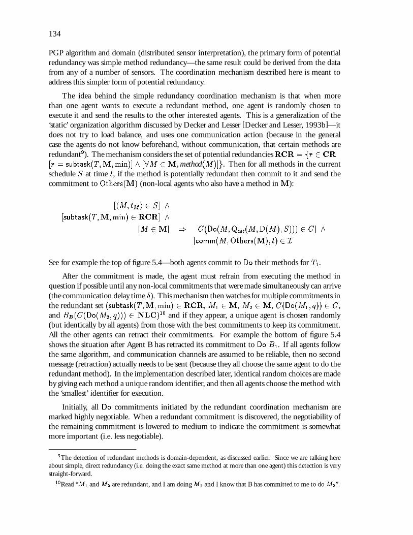
134

PGP algorithm and domain (distributed sensor interpretation), the primary form of potentialredundancy was simple method redundancy—the same result could be derived from the datafrom any of a number of sensors. The coordination mechanism described here is meant toaddress this simpler form of potential redundancy.

The idea behind the simple redundancy coordination mechanism is that when morethan one agent wants to execute a redundant method, one agent is randomly chosen toexecute it and send the results to the other interested agents. This is a generalization of the‘static’ organization algorithm discussed by Decker and Lesser [Decker and Lesser, 1993b]—itdoes not try to load balance, and uses one communication action (because in the generalcase the agents do not know beforehand, without communication, that certain methods areredundant9). The mechanism considers the set of potential redundanciesRCR = fr 2 CR j[r = subtask(T;M;min)] ^ [8M 2M;method(M)]g. Then for all methods in the currentschedule S at time t, if the method is potentially redundant then commit to it and send thecommitment to Others(M) (non-local agents who also have a method inM):

[hM; tM i 2 S] ^[subtask(T;M;min) 2 RCR] ^

[M 2M] ) [C(Do(M;Qest(M;D(M); S))) 2 C] ^[comm(M;Others(M); t) 2 I]

See for example the top of figure 5.4—both agents commit to Do their methods for T1.

After the commitment is made, the agent must refrain from executing the method inquestion if possible until any non-local commitments that were made simultaneously can arrive(the communication delay time �). This mechanism then watches for multiple commitments inthe redundant set (subtask(T;M;min) 2 RCR, M1 2M, M2 2M, C(Do(M1; q)) 2 C ,and BB(C(Do(M2; q))) 2 NLC)10 and if they appear, a unique agent is chosen randomly(but identically by all agents) from those with the best commitments to keep its commitment.All the other agents can retract their commitments. For example the bottom of figure 5.4shows the situation after Agent B has retracted its commitment to Do B1. If all agents followthe same algorithm, and communication channels are assumed to be reliable, then no secondmessage (retraction) actually needs to be sent (because they all choose the same agent to do theredundant method). In the implementation described later, identical random choices are madeby giving each method a unique random identifier, and then all agents choose the method withthe ‘smallest’ identifier for execution.

Initially, all Do commitments initiated by the redundant coordination mechanism aremarked highly negotiable. When a redundant commitment is discovered, the negotiability ofthe remaining commitment is lowered to medium to indicate the commitment is somewhatmore important (i.e. less negotiable).

9The detection of redundant methods is domain-dependent, as discussed earlier. Since we are talking hereabout simple, direct redundancy (i.e. doing the exact same method at more than one agent) this detection is verystraight-forward.

10Read “M1 and M2 are redundant, and I am doing M1 and I know that B has committed to me to do M2”.

135

Tmin

T1max

T2min

T4max

facilitates(T4,T1,0.5,0.5)A15

100

B15

100

Tmin

T3max

T1max

T2min

T4max

facilitates(T4,T1,0.5,0.5)

B4450

A15

100

B15

100

B35

100

Agent A's view after communication from B Agent B's view after communication from A

duration

quality

B3

Schedules:

B4

A1

t=5

B1

t=2 t=13

Commitments made from A to B:

Do(A1,100) [Mech #3]Commitments made from B to A:

DL(T4,50,5) [Mech #5]

Do(B1,100) [Mech #3]

Tmin

T1max

T2min

T4max

A15

100

B15

100

Tmin

T3max

T1max

T2min

T4max

B4450

A15

100

B15

100

B35

100

Agent A's view after recieveing B's commitments Agent B's view after receiving A's commitments

duration

quality

B3

Schedules:

B4

A1

t=5t=2 t=10

Commitments made from A to B:

Do(A1,150) [Mech #3]Commitments made from B to A:

DL(T4,50,5) [Mech #5]

Figure 5.4. A continuation of the previous figure. At top: agents A and B propose certaincommitments to one another via mechanisms 3 and 5. At bottom: after receiving the initialcommitments, mechanism 3 removes agent B’s redundant commitment.

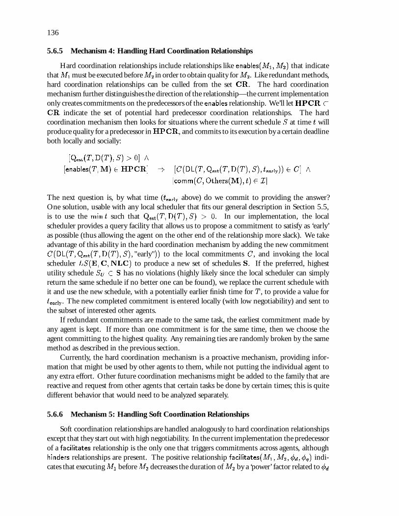
136

5.6.5 Mechanism 4: Handling Hard Coordination Relationships

Hard coordination relationships include relationships like enables(M1;M2) that indicatethatM1 must be executed beforeM2 in order to obtain quality forM2. Like redundant methods,hard coordination relationships can be culled from the set CR. The hard coordinationmechanism further distinguishes the direction of the relationship—the current implementationonly creates commitments on the predecessors of the enables relationship. We’ll letHPCR �CR indicate the set of potential hard predecessor coordination relationships. The hardcoordination mechanism then looks for situations where the current schedule S at time t willproduce quality for a predecessor inHPCR, and commits to its execution by a certain deadlineboth locally and socially:

[Qest(T;D(T ); S) > 0] ^[enables(T;M) 2 HPCR] ) [C(DL(T;Qest(T;D(T ); S); tearly)) 2 C] ^

[comm(C;Others(M); t) 2 I]

The next question is, by what time (tearly above) do we commit to providing the answer?One solution, usable with any local scheduler that fits our general description in Section 5.5,is to use the min t such that Qest(T;D(T ); S) > 0. In our implementation, the localscheduler provides a query facility that allows us to propose a commitment to satisfy as ‘early’as possible (thus allowing the agent on the other end of the relationship more slack). We takeadvantage of this ability in the hard coordination mechanism by adding the new commitmentC(DL(T;Qest(T;D(T ); S); "early")) to the local commitments C , and invoking the localscheduler LS(E;C;NLC) to produce a new set of schedules S. If the preferred, highestutility schedule SU 2 S has no violations (highly likely since the local scheduler can simplyreturn the same schedule if no better one can be found), we replace the current schedule withit and use the new schedule, with a potentially earlier finish time for T , to provide a value fortearly. The new completed commitment is entered locally (with low negotiability) and sent tothe subset of interested other agents.

If redundant commitments are made to the same task, the earliest commitment made byany agent is kept. If more than one commitment is for the same time, then we choose theagent committing to the highest quality. Any remaining ties are randomly broken by the samemethod as described in the previous section.

Currently, the hard coordination mechanism is a proactive mechanism, providing infor-mation that might be used by other agents to them, while not putting the individual agent toany extra effort. Other future coordination mechanisms might be added to the family that arereactive and request from other agents that certain tasks be done by certain times; this is quitedifferent behavior that would need to be analyzed separately.

5.6.6 Mechanism 5: Handling Soft Coordination Relationships

Soft coordination relationships are handled analogously to hard coordination relationshipsexcept that they start out with high negotiability. In the current implementation the predecessorof a facilitates relationship is the only one that triggers commitments across agents, althoughhinders relationships are present. The positive relationship facilitates(M1;M2; �d; �q) indi-cates that executingM1 beforeM2 decreases the duration ofM2 by a ‘power’ factor related to �d

137

and increases the maximum quality possible by a ‘power’ factor related to �q (see [Decker andLesser, 1993d] for the details). A more situation-specific version of this coordination mechanismmight ignore relationships with very low ‘power’. The relationship hinders(M1;M2; �d; �q) isnegative and indicates an increase in the duration of M2 and a decrease in maximum possiblequality. A coordination mechanism could be designed for hinders (and similar negativerelationships) and added to the family. To be proactive like the existing mechanisms, a hindersmechanism would work from the successors of the relationship, try to schedule them late,and commit to an earliest start time on the successor. Figure 5.4 shows Agent B making aD commitment to do method B4, which in turn allows Agent A to take advantage of thefacilitates(T4; T1; 0:5; 0:5) relationship, causing method A1 to take only half the time andproduce 1.5 times the quality.

5.7 Interfacing the Coordination Mechanism with the Local Scheduler

In our work on real-time AI problem solving prior to this dissertation we have found thatthe interface between the decision-maker and the real-time scheduler needs to be complex andbidirectional. We have argued that this interface can usefully be modeled as a negotiationprocess [Garvey et al., 1994]. In previous work on real-time scheduling, the interface betweenthe scheduler and the application has been very simple. It is usually assumed that the applicationpasses tasks on to the scheduler for scheduling and does not react when the scheduler is unable toschedule some tasks before their deadlines or only able to provide low quality solutions. A morecomplex interface is proposed in [Stankovic et al., 1989] that allows the application to ask what-ifquestions of the scheduler and modulate the behavior of the scheduler, however these ideas havenot been implemented to date. In our work on a complex, real-time, multi-agent problem-solverwe have found that a more bidirectional, negotiation-based interface is useful. Such an interfaceshould be useful in both multi-agent and complex, single-agent problem-solving environmentswhere there are many ways to solve a problem and also multiple criteria with which to judgethe potential solutions. I will briefly discuss the interface between higher-level decision-makingand lower-level scheduling and acting, described as a negotiation process between the schedulerand the decision-maker. I will discuss why each part of the interface is useful, whether it canbe implemented efficiently in a scheduler, and the effects of omitting that part.

As an example of what we mean by such an interface, consider a situation where multipleagents are working on a problem. Agent A has a method (Method A1) that enables theexecution of an important method at another agent B. At this point the decision-maker atAgent A realizes that it should try to get the scheduler to schedule Method A1. It can do this byassociating a do commitment with Method A1, meaning that it requests that the scheduler try tobuild schedules that execute Method A1. Agent A’s scheduler returns a schedule that completesexecuting Method A1 at time 7. The decision-maker at Agent A tells other decision-makersthat it can commit to giving them the result of Method A1 at time 8 (allowing time forcommunication to occur). At the second agent B, the decision-maker receives this message andpasses it along to the scheduler, which reports back that time 8 is too late—the result is neededby time 6. Agent A’s decision maker is informed of this feedback, and Agent A again invokesits scheduler, now with a deadline commitment to complete Method A1 by time 5 (to allowtime for communication). Agent A’s scheduler returns a schedule that commits to completingMethod A1 by time 5 and Agent A communicates this information to the other agent, which

138

is now able to complete its method by the deadline. Meeting the tighter schedule mightbe possible only by making other tradeoffs—lowering the local quality produced or violatingsome other commitment. In this example, the decision-maker and scheduler at each agent aresemi-autonomous subsystems, communicating bidirectionally and sometimes requiring morethan one step to arrive at a satisfactory solution.

Given that significant communication in both directions is required in our layeredapproach, an obvious question is why have separate subsystems. There are many reasonswhy a distinct separation should exist between such a scheduler and decision-maker, includingat least modularity, efficiency and reusability. Modularity suggests that separate functionalityshould be kept in separate modules with clearly defined interfaces. In general it is difficult for allcurrent problem solving criteria to be encapsulated into an evaluation function and transmittedto the scheduler, because deciding what to do is a evolving computational process. From thescheduler’s perspective, transmitting all potentially useful information about a schedule is alsodifficult and inefficient. Another reason why a separation should exist is that the subsystemswork at different levels of abstraction. One of the roles of the decision maker is to constrain thesearch done by the scheduler, for example, by using commitments to tell the scheduler whatparts of the task structure to focus on. While it is possible for the scheduler to use all availableinformation to make such decisions itself, for efficiency reasons it is useful to have the decisionmaker constrain the search space for the scheduler. Another reason for separating schedulingand decision-making is that scheduling is a more generic activity and it should be possible toreuse schedulers in multiple applications. It is undesirable to reproduce a scheduler each timea new problem area is investigated.

I will discuss the scheduler/decision maker interface using examples from two differentpoints-of-view: multi-agent environments such as those that have been addressed in thisdissertation, and hard real-time environments that might be addressed in the future. The twopoints-of-view are not necessarily inconsistent with one another.

Multi-agent scenarios.

In the multiagent scenarios I discussed in Section 5.5, each method is executable by exactlyone agent, however several agents may have identical methods for achieving quality for thesame task. The goal of the coordinated decision-makers is to work together to produce thehighest possible quality for as many task groups as possible, i.e., each attempts to maximizethe global utility measure U(E) =

PT 2EQ(T ;D(T )). This is not straightforward, because

each agent sees only some part of the total task structure, and it may be the case that no agentsees the entire structure. Thus a decision maker cannot simply ask the scheduler to optimizethis global criteria. One kind of information that agents can communicate to one anotheris information about the task structures that they see (i.e., GPGP mechanism 1: updatingnon-local viewpoints). The decision-makers are responsible for coordinating their activity soas to avoid redundant method execution and allow relationships that extend across agents tobe exploited or avoided as appropriate using the other GPGP coordination mechanisms. Therole of the scheduler is to schedule execution of local methods according to criteria providedby the decision-maker.

Real-time scenarios.

In the real-time scenarios that we are working with, task groups arrive continuously, andrequire the use of multiple reusable physical resources (motorized tables, robot arms) and

139

consumable resources. There are often not enough resources to complete all task groups,but the decision-maker still attempts to maximize its total utility. Each task group mayhave a different maximum payoff I(T ), and the decision-maker tries to maximize U(E) =P

T 2E I(T )Q(T ;D(T )). Here the criteria are known but the best mix of problems to solveis not. The role of the scheduler here is to endorse the execution of time-critical control codeson multiple hardware platforms, using shared, private, and consumable resources. Some taskgroups, representing periodic, maintenance, or operating system activities, will be constantlypresent and their execution will be absolutely guaranteed.

5.7.1 Scheduler Inputs

The decision-maker proposes to the scheduler that a solution to each newly arriving taskgroup be added to the schedule of methods to be executed. A basic request to the scheduler(its input) consists of four things: the task structures to be scheduled, a set of commitments, aset of non-local commitments, and a runtime indication.

Tmin

Tmax

Tmin

Tmax

Tmax

Tmin

Tmax

B745

C5

35

D5

40

E3

20

F8

30

A820

Deadline Commitment: Q=45,T="Early"

Nonlocal Commitment: Q=40, T=6

Q-effect: 0.5, D-effect: 0.5

Deadline: 25

Tmin

task with quality accrual function min

subtask relationship

enables relationship

method (executable task)

facilitates relationship

namedurationquality

Figure 5.5. An example of a complete input specification to the scheduler.

The task structures to be scheduled ES , should include some indication of what aspectsof those structures have changed since the scheduler was last invoked. If we write Bt

A(X) toindicate what agent A believes at time t about X , then the scheduler at agent A at time t hasaccess to Bt

A(E), and BtA(E) nBt�1

A (E).The set of commitments C are constraints that the invoker would like the scheduler to try

to satisfy. We have defined three types of commitments:

� C(Do(T; q)) is a commitment to ‘do’ (achieve quality for) T and is satisfied at the timet when Q(T; t) � q. A ‘don’t’ commitment is also possible.

� C(DL(T; q; tdl)) is a ‘deadline’ commitment to do T by time tdl and is satisfied atthe time t when [Q(T; t) � q] ^ [t � tdl]. A C(Do(T; q)) is really shorthand forC(DL(T; q;D(T ))).

140

� C(EST(T; q; test)) is a ‘earliest start time’ commitment11 to not begin work on T beforetime test and is satisfied at the time test iff 8t � test; Q(T; t) � q.

The importance of local commitments such as these are as soft constraints on the possiblesolutions. Any scheduler that can schedule real-time method executions can already deal withhard constraints such as deadlines and earliest start times. Hard commitments can be used toprovide guarantees [Cheng et al., 1988] by requiring commitments to be satisfied in all validschedules.

Soft commitments are needed to handle the coordination of multiple agents where thereis more than one way to solve a task or where there are soft coordination relationships such asfacilitates. They are also useful in real-time systems, as shown by Spring’s use of endorsements[Cheng et al., 1988] to indicate commitments that may only be violated when more importanttasks arrive. When invoking the scheduler in a query mode, the decision-maker may alsosupply the symbolic values ‘early’ for a deadline commitment and ‘late’ for an earliest start timecommitment, which indicates to the scheduler that it should attempt to satisfy the commitmentas early or late as possible.

If a scheduler does not provide the ability to specify soft commitments, it is possible insome situations for the decision-maker to achieve the same results by repeated execution ofscheduler queries using hard commitments (even changing the task structure, if need be). Webelieve it will always be more efficient to add the ability to interpret soft constraints to thescheduler than to play guessing games by invoking the scheduler multiple times.

The set of non-local commitments NLC are commitments that the scheduler can assumewill be satisfied. These are of the form of the commitments mentioned above and tell thescheduler to expect to receive the indicated results at the indicated time. In general, thescheduler would not concern itself with the reliability of this information, which is would bedetermined by the decision-maker. A sophisticated scheduler might concern itself with thereliability of these non-local commitments, but most schedulers assume this information isreliable.

In multi-agent problems, non-local commitments can be used to communicate workthat will be done by other agents. This component is necessary for achieving coordinatedbehavior in complex domains. These non-local commitments might be created at run timeby the decision-makers, or they might be derived from pre-defined ‘social laws’ [Shoham andTennenholtz, 1992] that all agents agree to, or are constructed to, satisfy. The most importantcomponent of an agent’s particular organizational role is the set of non-local commitments itforces the agent to adhere to. Another effect of NLCs in multi-agent problems is the triggeringof non-local effects (coordination relationships); each non-local deadline commitment, forexample, implies an earliest start time on the ‘affected’ end of any relationships. For hardrelationships like enables this implies a hard earliest start time; for soft relationships it actuallyexpands the search space (since each affected task can be started either before or after the earlieststart time with different results).

In real-time problems as well, non-local commitments are important. In our exampledomain not all of the hardware is under the control of the real-time operating system scheduler,

11In fact this is more general than a standard earliest start time constraint, in that it allows some nonzeroamount of work to be done on T as long as quality does not go above the threshold. Standard earliest start timescan be modeled with a q value of 0.

141

in particular the robot arms run on separate hardware with a separate specialized executioncontroller. The only way for the RT scheduler to function is to allow the robot hardware tomake non-local commitments (in this case, worse-case execution time guarantees) about certainphysical activities that are not directly under the control of the real-time scheduler.

Another way to look at non-local commitments is that they give the decision-maker a wayto only partially flesh out a task structure and to direct a scheduler’s search, potentially makingit more efficient. NLCs on elements of MAX (OR) nodes provide initial lower bound ‘best’estimates, while NLCs on MIN (AND) elements provide upper bounds. Both types can beused to prune search in time-constrained situations—NLC’s below MAX (OR) nodes couldprune all their siblings from local consideration; NLCs below MIN (AND) nodes can onlylocally prune below the node with the NLC. For example, if the task ‘get food for the party’consists of the subtasks ‘buy prepared food’ OR ‘make food from leftovers’, then if anotheragent commits to ‘buy prepared food’ I can prune this entire substructure from my schedule.On the other hand, if ‘get food for the party’ consists of the subtasks ‘buy ingredients’ AND‘make food from ingredients’, then a non-local commitment to ‘buy ingredients’ prunes thatsubtask (and any below it) only; I still need to schedule to ‘make food from ingredients’.

Another potential use for non-local commitments is to allow the decision-maker to directthe search of the scheduler. The decision-maker can use non-local commitments to askquestions such as, assuming quality is achieved in this part of the task structure, how could wetake advantage of that in other parts of the task structure. This could be useful in situationswhere the cost of the information gathering associated with expanding a task structure ispotentially large. It could also be used in situations where the scheduler has successfullyproduced a schedule to satisfy one part of a task structure and the decision-maker now wantsto focus the schedulers attention on another part that can begin execution when the previouslyscheduled work is completed. In time-constrained situations such non-local commitmentscan reduce search for the scheduler by allowing it to prune committed portions of the taskstructure.

Various mechanisms for controlling the runtime of the scheduler can include: a harddeadline by which the scheduler should complete; a satisficing value for a schedule (thescheduler completes when a schedule of at least this value is found); or a decision-theoretictradeoff function that indicates the added value of spending time finding better schedules versusexecuting the first element of the current schedule[Russell and Wefald, 1991]. In non-real-timescenarios, this might not be particularly important as long as the runtime of the scheduler issmall compared to the grain size of application tasks. In real-time scenarios it is crucial to atleast be able to predict the worst-case performance of the scheduler.

5.7.2 Scheduler Output

The output from the scheduler after an invocation should include at least one valid schedule,a list of satisfied commitments, a list of violated commitments with alternatives, an indicationof tasks that should be scheduled but are not, and an indication of the value of each returnedschedule with respect to some fixed set of criteria.

A set of valid schedules S is returned that do a satisfactory job of satisfying the problemgiven to the scheduler. An individual schedule S 2 S consists of at least a set of methodsand start times: S = fhM1; t1i; hM2; t2i; : : : ; hMn; tnig. This output is of course necessary,

142

and forms the initial proposal in the negotiation process. The remaining items provide anexplanation of this proposal.

The next three items returned (satisfied commitments, violated commitments with alter-natives, and multi-criteria schedule values) are not necessary for the scheduler to provide,because they can all be derived mathematically from the schedule itself and the set ofnon-local commitments. However, for practical implementations, the scheduler often has thisinformation at hand, or can collect it during schedule generation, and it would be expensive torecompute.

The set of input commitments that are satisfied in a schedule Satis�ed(S) is returned(8S 2 S;Satis�ed(S) � C). If the scheduler supports symbolic local commitments like ‘early’deadline commitments and ‘late’ earliest start time, then it must also supply an indication ofwhen the commitment is expected to be satisfied in the schedule SatTime(C;S). For example,if C1 = DL(T; q; ‘early’) and C1 2 Satis�ed(S) then SatTime(C;S) = min t � D(T ) s.t.Qest(T; t; S) � q.

The set of input commitments that are violated in a schedule Violated(S) is returned. Foreach violated commitment, a proposed modification to the commitment that the scheduler isable to satisfy (Alt(C;S)) is also returned. For earliest start time and deadline commitmentsthis involves a proposed new time and/or minimum quality. For do/don’t commitments thisinvolves a recommended retraction or a reduced minimum quality value. For example, fora violated deadline commitment C(DL(T; q; tdl)) 2 Violated(S) the function Alt(C;S)returns an alternative commitment C(DL(T; q; t�dl)) where t�dl = min t such that Q(T; t) � qif such a t exists, or NIL otherwise.

The knowledge that certain commitments are satisfied or violated is absolutely necessaryto the decision-maker that uses commitments, regardless of the domain.

An indication of the “value” of the schedules that were returned according to several objectivecriteria. Some of the objective functions that can be measured include the total quality forall scheduled task groups,12 the number of task groups that do/do not complete before theirdeadline, the amount of slack time available in the schedule to allow easy scheduling of newtasks and/or allow time for tasks to take longer than expected to run, and the number (orweighted value) of the commitments that are not satisfied in the schedule (our decision criteriawas described in Section 5.6.1).

Complex real problems invariably involve multiple evaluation criteria that must be balancedwith one another; we view this balancing as the role of the decision-maker, and the schedulerattempts to maximize the current criteria, often returning multiple schedules (e.g., one thatbest satisfies each of the current criteria.) While the ability to evaluate a schedule with respectto certain criteria could be implemented outside of the scheduler, the ability to attempt tooptimize certain criteria can only be placed in the scheduler.

In our multi-agent system, for example, Agent A’s decision-maker might make a commit-ment to Do(M1; q), and tell other agents. As time passes, Agent A will need to make a decisionabout whether to abandon the commitment—perhaps the scheduler finds a ‘better’ schedulethat bypasses the execution of M1. The scheduler cannot make this decision because it canonly evaluate the schedule via local criteria. If another agent B uses the result of M1 to producea very high quality solution that A could not produce alone, B’s decision-maker can notify A’s

12This could be a weighted sum if task group importance varies, or some more complex function if desired.

143

decision-maker about the updated utility of the commitment. The decision-maker is now ina much better position to decide whether to abandon the local commitment to M1 than thescheduler is, and the process did not involve the agent’s exchanging all of their knowledge andall of their current schedules.

A real-time example of changing criteria can occur when time pressure is not constant.Under normal processing, the scheduler may process all task groups, attempting to producemaximal quality. However, when feedback from the scheduler indicates that it is unableto successfully schedule all task groups, the decision-maker may switch to a ‘time-pressured’mode where the scheduler is directed to only produce minimum quality for every task. Such‘mode-changing’ behavior can be directed by a decision-maker only by using feedback fromthe scheduler. Other work has shown such mode-changing behaviors as pre-compiled into thescheduler for efficiency purposes[Hayes-Roth et al., 1988].

A minimal list of tasks in the task structure that the schedule is not providing quality forbut would need to have quality to allow their task group to achieve non-zero quality. Such taskscan result from the scheduler not having any local methods to generate quality for the tasks(either because the task structure is distributed across agents and those tasks have methods atsome other agent(s), or because the agent has not yet done the information gathering necessaryto determine what methods are available for the task.) Such tasks can also result from thescheduler not being able to schedule the execution of all methods known to it because ofdeadlines or other constraints.

0 2 4 6 8 10 12 14 16 18 20

A: Q=20, D=8

B: Q=45, D=7 F: Q=45, D=4

B: Q=45, D=7 D: Q=40, D=5 F: Q=45, D=4Final Quality: 40Total Duration: 16

Commitment satisfied:at time 7

Commitment satisfied:at time 7

Final Quality: 40Total Duration: 11

Final Quality: 20Total Duration: 8

Commitment violated:No alternative

Figure 5.6. An example of the output of the scheduler for the example problem given above.

A summary of the output of the scheduler for the example problem given above is shownin Figure 5.6. In this example three schedules are returned. The bottom one is the schedulegenerated by the minimum duration generator and produces a fast, low quality result, violatingthe given deadline commitment because no quality is ever generated for the committed task.The middle schedule is generated by the highest quality generator and produces the highestpossible quality in the fastest possible time, satisfying the deadline commitment at time 7.The top schedule is generated by the minimum nonlocal reliance generator and produces thehighest quality possible completely locally, not relying on the given nonlocal commitment,also satisfying the deadline commitment at time 7. Which of these schedules is chosen by thedecision-maker depends on the current evaluation criteria. If the fastest possible, acceptable

144

result is desired, perhaps because of a large workload of other tasks, then the bottom scheduleis chosen. If the best possible result in the minimum possible time is desired, the the middleschedule is chosen. If the best possible result that does not rely on other agents is desired(possibly because of other work that those agents need to do or a concern about the otheragent’s reliability) then the top schedule is chosen.

5.7.3 Interfacing the Coordination Mechanism with the Local Scheduler: Discussion

We will first return to the main reasons for a bidirectional interface separating schedulingfrom decision making—reusability, modularity, and efficiency.

Of the various reasons for developing a complex bidirectional interface, the reusabilityargument is the most clear. A scheduling component that attempts to find optimal methodexecution times for arbitrary task structures and evaluation criteria is useful in many domains,regardless of whether they have real-time or distributed problem solving components. Amore important related question is whether the extra capabilities required by this interfacecan be provided cheaply by an otherwise efficient, reusable scheduler. Examining the inputcharacteristics, we find that the input task structures are not much more than the specificationof the problem to be solved, and that handling these constraints would not be an additionalburden to a standalone scheduler. Commitments, amounting to preferred (soft) deadlines andearliest start times are also part of standard real-time scheduling specifications. So too are themechanisms for controlling the runtime of the scheduler, for any scheduler that can schedulereal-time tasks with deadlines. The only potentially unique feature is the input of non-localcommitments. If non-local commitments are always taken at face value (no lies) then they canbe used for making more efficient searches, as discussed earlier.

Examining the reusable scheduler’s output characteristics for efficient implementation, wefind the first two—the schedules themselves and which commitments are satisfied when—tobe non-controversial parts of almost any real-time scheduler. So too is the list of violatedcommitments, but perhaps not the generated alternatives. Generating alternatives to violatedcommitments on executable methods is trivial—just look in the generated schedule and returnthe actual execution if found, or suggest retraction of the commitment otherwise. Generatingalternatives for high-level task commitments may be somewhat more complex, depending onthe internal structure of the scheduler and what information is efficiently available. As wementioned earlier, this output characteristic was assigned to the scheduler because it is usuallymore efficient to compute there, but it can be (inefficiently) computed by the decision makerfrom the schedule and non-local commitments themselves if necessary. The same thing istrue of schedule evaluations under multiple criteria—it is our experience that the schedulercan more efficiently calculate these evaluations that the decision maker. The scheduler usuallyhas already computed these evaluations as part of its search process. The most unique andpotentially expensive output characteristic is the production of a task list for which the schedulerdesires quality but cannot produce. This behavior enables several sophisticated responses inmulti-agent systems, such as contracting behavior on the part of the decision maker on behalf ofthe scheduler, but is not part of the standard definition of scheduling problems and undoubtedlycauses extra overhead. We plan to analyze how this behavior can be efficiently provided andunder what circumstances it is useful in future work.

The other two reasons for a complex bidirectional interface, efficiency and modularity, areclosely tied. Efficiency is primarily the ability to search on, or attempt to optimize, specific

145

criteria effectively. Defining a carefully delimited scheduling problem, and even limited searchcriteria, allows for the construction of a efficient scheduler. In fact, multiple schedulers mightbe constructed, each optimized to search (perhaps in parallel) under a different criteria (bestquality, least violated commitments, earliest finish time). This leads directly to the modularityargument—that in general it is difficult to encapsulate all problem solving criteria into a singleevaluation function, and deciding on the correct criteria is an evolving computational process(to be handled by a separate decision maker, we argue).

5.8 Summary

This chapter discussed my third contribution: the development of the Generalized PartialGlobal Planning family of coordination mechanisms. The GPGP algorithm family specifiesthree basic areas of the agent’s coordination behavior: how and when to communicate andconstruct non-local views of the current problem solving situation (answered by Mechanism1, update non-local views); how and when to exchange the partial results of problem solving(answered by Mechanism 2, communicating results); how and when to make and breakcommitments to other agents about what results will be available and when (Mechanisms 3,4, and 5, handling simple redundancy and hard and soft relationships). Each agent also hasa heuristic local scheduler that decides what the agent should do next, based on its currentview of the problem solving situation (including the commitments it has made), and a utilityfunction. The coordination mechanism supplies non-local views of problem solving to thelocal scheduler, including what non-local results will be available locally, and when they will beavailable. The local scheduler creates (and monitors the execution of) schedules that attempt tomaximize group quality through both local action and the use of non-local actions (committedto by other agents).

GPGP attempts to extend PGP in several ways. First, it permits more agent heterogeneityand, when possible, more scheduling autonomy. Agents are still considered to be cooperative(working with a shared global utility criteria), but GPGP permits agents to have different localviews (letting the scheduler work with partially global plans (really schedules). In the originalPGP algorithm agents generally communicate complete schedules (at a single a priori fixed levelof abstraction), whereas GPGP agents only communicate scheduling commitments to particularactions (at any dynamically decided level of abstraction). Agents can be heterogeneous in theircapabilities as well—some agents can be faster at certain tasks or have unique capabilities(methods). However, GPGP is a family of coordination mechanisms and does not addressproblems of heterogeneous systems such as created shared languages for communication. GPGPis useful in cooperative distributed problem solving (CDPS) situations, but the current set ofmechanisms would be vulnerable to lying in a non-cooperative multi-agent situation.

Secondly, GPGP extends PGP to dynamic environments and problem solving architectureswhere planning (scheduling) at a single level of detail is not practical. This extension includescommunicating meta-level information at varying levels of detail and reacting appropriately tosituations where there is more than one way to accomplish a high level task.

The third GPGP extension is to real-time problem solving, with the addition of harddeadlines and more flexible temporal commitments. However, the algorithm is only ‘real-time’in the same sense as the underlying local scheduler (developed by Garvey [Garvey and Lesser,1994]), and not in the strong sense of guaranteed computation like the Spring scheduler

146

[Stankovic et al., 1989] (how these all can work together is a future research direction, see alsothe discussion in Section 5.7).

Because GPGP is a cooperative, team-oriented mechanism, it assumes that no agent has aconsistently better view of problem solving (either because of the problem-solving algorithmor by some imposition of the environment). Our approach views the coordination mechanismas modulating local control, not supplanting it—a two-level process that makes clear thedistinction between coordination behavior and local scheduling, and different from past andpresent Durfee work. It is also different from Corkill’s work (which also had distinct localcontrol [Corkill and Lesser, 1983]) in that it is dynamic in nature. This separation also allowsGPGP to take advantage of recent advances in the planning and scheduling of computations.

GPGP mechanisms are reactions to the presence and quantitative features of coordinationrelationships. Coordination relationships, as they arise from the general task environmentmodel, have domain-independent definitions. These relationships have quantitative propertiessuch as how likely they are to appear, how difficult they are to detect, and how significant theireffect is. A coordination algorithm defined in terms of detecting the existence and propertiesof CRs, and producing scheduling constraints, is more general than one written for a specificapplication such as the DVMT. Both domain-independence and modularity will allow forresearchers and application designers to share ideas more easily.

GPGP is a family of algorithms—each of the five mechanisms described here are param-eterized independently (the first two have three possible settings and the last three can be inor out) for a total of 72 combinations. For example, one specific family member that we willuse experimentally in the next chapter is named the “balanced” algorithm. The “balanced”algorithm has Mechanisms 3, 4, and 5 ‘on’, updates ‘some’ non-local views (Mechanism 1),and communicates commitments and finished task groups (Mechanism 2). Many of thesecombinations do not show significantly different performance in randomly generated episodes,as will be discussed in the next chapter, although they will allow for fine-tuning in specificapplications. More mechanisms can (and have) been added to expand the family, but thefamily can also be enlarged by making each mechanism more situation-specific. For example,mechanisms can have their parameters set by a mapping from dynamic meta-level measurementssuch as an agent’s load or the amount of real-time pressure. Mechanisms can be ‘in’ or ‘out’for individual classes of task groups, or tasks, or even specific coordination relationships, thatre-occur in particular environments. The cross product of these dynamic environmentalcues provides a large but easily enumerated space of potential coordination responses that areamenable to the adaptation of the coordination mechanisms over time by standard machinelearning techniques or case-based reasoning approaches. Such extensions fall under the headingof Future Work (Chapter 7). In the experimental section of dissertation (Chapter 6) we willonly consider the coarsest parameterization of the mechanisms.

In the next chapter we will evaluate and show the performance of these mechanisms, usingseveral sets of experiments that deal with performance of the GPGP mechanisms in differentenvironments, using a real implementation (running in Common Lisp on multiple platforms,and being used by more than one person). The implementation uses as submodules a realimplementation of Garvey’s Design-To-Time real-time scheduler [Garvey and Lesser, 1994].

C H A P T E R 6

EXPERIMENTS IN GENERALIZED PARTIAL GLOBAL PLANNING

“You doubt what I wrote? Let me show you.” We now understand that what theProfessor is asking us to watch is related to the figure [in his scientific paper]. We thusrealize where this figure comes from. It has been extracted from the instruments of thisroom, cleaned, redrawn, and displayed. We also realize, however, that the imagesthat were the last layer in the text, are the end result of a long process in the laboratorythat we are now starting to observe.

We are no longer asked to believe the text we read in ‘Nature’; we are now asked tobelieve our own eyes : : :Do we see more or less than before? We can see more, since wehave before our eyes not only the image but what the image is made of. On the otherhand we see less because now each of the elements that makes up the final graph couldbe modified so as to produce a different visual outcome. : : :The Professor, for instance,is swearing at the gut saying it is a ‘bad gut’.

A guinea pig is placed on a table, under surgical floodlights, then anaesthetised,crucified, and sliced open. : : :Suddenly, we are much further from the paper worldof the article. We are now in a puddle of blood and viscera, slightly nauseated by theextraction of the ileum from this little furry creature. In the last chapter, we admiredthe rhetorical abilities of the Professor as an author. Now, we realize that many otherabilities are required in order to write a convincing paper later on. The guinea pigalone would not have been able to tell us anything : : : it was not mobilisable into atext and would not help to convince us. Only a part of its gut, tied up in the glasschamber and hooked up to a physiograph, can be mobilised in the text and add to ourconviction. Thus, the Professor’s art of convincing his readers must extend beyond thepaper to preparing the ileum, to calibrating the peaks, to tuning the physiograph.

— Bruno Latour, Science in Action

These experiments involve a complete implementation of GPGP and a separately developedreal-time local scheduler [Garvey and Lesser, 1993, Garvey et al., 1994]. We will showhow to decide when a particular mechanism (and thus GPGP) is useful, how some familymembers perform relative to a centralized algorithm,and what the space of possible coordinationalgorithms looks like for the five mechanisms currently defined. We analyze the performance ofthis family of algorithms through simulation in conjunction with the heuristic real-time localscheduler and randomly generated abstract task environments.

In these environments, the agents attempt to maximize the system-wide total utility (aquantity called ‘quality’, described later) by executing sequences of interrelated ‘methods’. Theagents do not initially have a complete view of the problem solving situation, and the executionof a method at one agent can either positively or negatively affect the execution of other methods

148

at other agents. We will show examples of the effect of the environment on the performanceof a GPGP family member, and show an environment where family member A is better thanB, and a different environment where B is better than A. We will return to the demonstrationof meta-level information being more useful when there is a large amount of variance betweenepisodes in an environment.

In this final section we will discuss experiments we have conducted with our implementationof these ideas:� How should we decide when the addition of a particular mechanism is warranted?

� What is the performance of a system using all the mechanisms compared to a systemthat only broadcasts results? Compared to a system with a centralized scheduler?

� What is the performance space of the GPGP family, as delineated by the five existingmechanisms?

As we have stated several times in this dissertation, we do not believe that any ofthe mechanisms that collectively form the GPGP family of coordination algorithms areindispensable. What we can do is evaluate the mechanisms on the terms of their costsand benefits to cooperative problem solving both analytically and experimentally. This analysisand experimentation takes place with respect to a very general task environment that doesnot correspond to a particular domain. Doing this produces general results, but weaker thanwould be possible to derive in a single fixed domain because the performance variance betweenproblem episodes will be far greater than the performance variance of the different algorithmswithin a single episode. Still, this allows us to determine broad characteristics of the algorithmfamily that can be used to reduce the search for a particular set of mechanism parametersfor a particular domain (with or without machine learning techniques). We will also discussstatistical techniques (e.g. paired-response) to deal with the large between-episode variancesthat occur when using randomly-generated problems.

The first section of this chapter describes a set of experiments using a very simplesimulation and task structure that looks only at the effect of the facilitates relationship onagent performance—in particular, the effect of the power of the relationship and the likelihoodof its existence. The rest of the chapter is devoted to an exploration of the performance of theGPGP family of coordination mechanisms as described in the previous chapter.

6.1 Initial Experiments: The Effect of Facilitation Power and Likelihood

The simulation used in this first chapter section is driven by the environment, task, andagent characteristics we discussed in Chapter 3; the tasks represent abstract computationsand their structure was a simple one-level-deep AND hierarchy. Experiments using the fullTÆMS framework will be discussed in the rest of the chapter, beginning in Section 6.2. In theexperiments below, there were two abstract task groups. One group of tasks had a mean timebetween subtask arrivals of 40% less than the other. Each task arrives uniformly randomlyat an agent. Facilitation relationships are generated between tasks with a base probabilitythat decreases linearly with the difference between task arrivals1. For example, if there are

1The reader should not be worried about ‘linear’ vs. ‘exponential’ here. An experiment not reported hereshowed that in an environment where the probability of a facilitates relationship drops off exponentially insteadof linearly, the system response characteristics are similar to a linear environment with the same number of detectedrelationships.

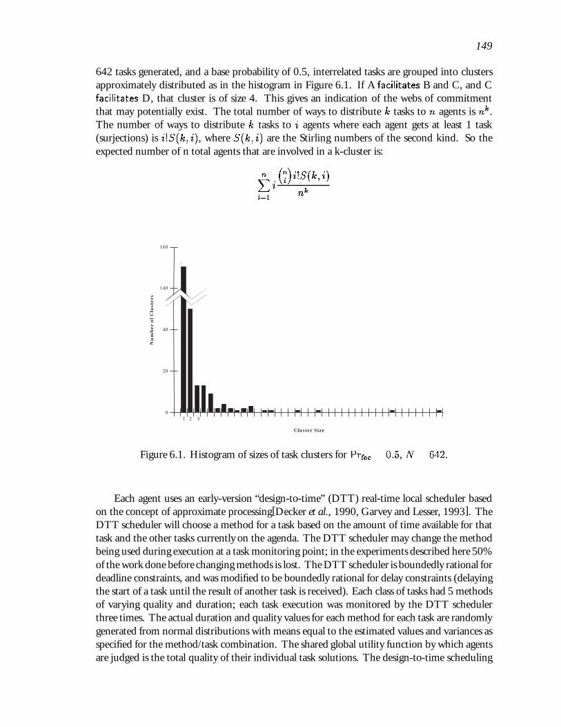
149

642 tasks generated, and a base probability of 0.5, interrelated tasks are grouped into clustersapproximately distributed as in the histogram in Figure 6.1. If A facilitates B and C, and Cfacilitates D, that cluster is of size 4. This gives an indication of the webs of commitmentthat may potentially exist. The total number of ways to distribute k tasks to n agents is nk .The number of ways to distribute k tasks to i agents where each agent gets at least 1 task(surjections) is i!S(k; i), where S(k; i) are the Stirling numbers of the second kind. So theexpected number of n total agents that are involved in a k-cluster is:

nXi=1

i

�ni

�i!S(k; i)

nk

Cluster Size

Nu

mb

er o

f C

lust

ers

160

140

40

20

01 2 3

Figure 6.1. Histogram of sizes of task clusters for Prfac = 0:5, N = 642.

Each agent uses an early-version “design-to-time” (DTT) real-time local scheduler basedon the concept of approximate processing[Decker et al., 1990, Garvey and Lesser, 1993]. TheDTT scheduler will choose a method for a task based on the amount of time available for thattask and the other tasks currently on the agenda. The DTT scheduler may change the methodbeing used during execution at a task monitoring point; in the experiments described here 50%of the work done before changing methods is lost. The DTT scheduler is boundedly rational fordeadline constraints, and was modified to be boundedly rational for delay constraints (delayingthe start of a task until the result of another task is received). Each class of tasks had 5 methodsof varying quality and duration; each task execution was monitored by the DTT schedulerthree times. The actual duration and quality values for each method for each task are randomlygenerated from normal distributions with means equal to the estimated values and variances asspecified for the method/task combination. The shared global utility function by which agentsare judged is the total quality of their individual task solutions. The design-to-time scheduling

150

algorithm used by each agent ensures that under normal circumstances (a required utilization(system load) of less than 3) less than 2% of the tasks ever miss a deadline. This is a propertyof the existence of low cost/low quality approximations.

Observations in the experiments that follow are made from average responses over 5statistically generated runs of 1000 simulated world time units. The number of tasks thatare actually generated depends on their arrival rate, which was varied. We also varied the apriori likelihood (Prfac) of a facilitates relationship between two tasks of the same class andthe significance of the effect it has on the time of the facilitated tasks (called the power of theCR and measured by the percent reduction in time facilitated).

Each run consists of two sets of 4 agents. Each of the two agent-sets receives exactly thesame set of tasks at exactly the same times—one agent-set uses the original DTT schedulingalgorithm and no communication, the other agent-set uses the DTT scheduling algorithmmodified to be boundedly rational with respect to delay constraints and to always detect andcommunicate coordination relationships. Each of the four agents in each agent-set receivesprecisely the same set of tasks as its counterpart in the other agent-set. The coordinating agentscalculate delays as described in Figure 6.2. If a commitment fails, the coordinating agentssimply break the failed commitment.

The primary performance metric in the experiments presented here is the percentageincrease in quality between each pair of agents that received the same task set (a pairedresponse), and then averaged across the agent pairs. This metric is indicated in the figuresby APQI (average percent quality increase). The other variable that was manipulated was themean time between arrivals of the tasks; we can then compare relative increases in quality basedon the average utilization required by that set of tasks. When the average required utilization isgreater than 1, it means that it is impossible to complete all tasks without approximating someof them.

There are three characterizations of this simulated environment that make it different fromthe actual environment of a system such as the DVMT:

� In interpretation environments like the DVMT, not all tasks need to be done, but in thissimulation, in this section, they do. The rest of the chapter will discuss a more complexsimulation where not all work needs to be done.

� This simulation assumes that approximating a result has only a local effect on quality, asopposed to reducing the quality of a whole group of related tasks.

� This simulation does not contain a model of the relationship between the fact that atask does or doesn’t need to be done, and the fact that a facilitates relationship does ordoesn’t exist.

On the other hand, our measurements are against a design-to-time real-time schedulingalgorithm that likewise does not take these factors into account. The addition of these extracharacteristics to the task structure requires the addition of new coordination relationships(especially subtask). The second part of this chapter (starting at Section 6.2) will discussGPGP using the full TÆMS task structure framework.

6.1.1 Calculating Delays

How do we compute how long to delay a task B that is facilitated by a task A? For example(see Figure 6.2), if

151

� utility is a function of result quality only (as opposed to a function of both quality andmissed deadlines)

� the local scheduler does not assure the minimal quality of a task result

� facilitates affects only the durations of tasks directly

then agents must attempt to produce their highest quality solutions. Suppose there are severaldifferent tasks Bi such that A facilitates each Bi. If we estimate the latest start time for eachtask B in order to produce a highest quality solution, and estimate the finish time for task A,then all tasks B with latest start times after the estimated finish of A (B2 and B3 in the figure)should be delayed to the minimum latest start time of those tasks (B2 in Figure 6.2; timesmust be calculated taking communication time into account if it is substantial). If the localscheduler were boundedly rational with respect to quality constraints, then the estimate of thelatest start time of B could be modified by (made later by) the estimated effect of the facilitatesrelationship for the maximally assured minimal quality of the result of task A.

B1

A

B3

B2

Task Deadline

Task A Estimated Finish Time (max quality)

Task Latest Start Time (max quality)Minimum Latest Start Time

Extra Time (slack)

Delay

Figure 6.2. Calculating Delays

6.1.2 A Simple Model of the Utility of Detecting Facilitates

When should an agent test for a facilitation relationship? An agent can potentially test forthe presence of the facilitates relationship between any new local task and the tasks it knowsabout from other agents. The costs per task here include the processing cost of testing forthe relationship between two tasks and the cost of communication to get more informationif the test result is too uncertain (Cdetect). Note that the test itself is domain specific, eventhough the facilitates relationship is general. If the relationship is present, the benefits include

152

some increased utility (reduction in time, increase in quality of the facilitated task) (Bfac).The benefits will accrue fully only if the scheduling constraints implied by the new detectedrelationship can be incorporated, and only if the facilitating task is accomplished.2 Costs arealso incurred when the relationship is present, including the direct costs of communicating theresult, adding the scheduling constraints, and updating the models of each others’ tasks, and theindirect costs of delaying some tasks (Cfac). Using the a priori likelihood Prfac of a facilitates

relationship from the environmental model, we can build an expression for the form of theexpected utility of the relationship, Prfac �(Bfac � Cfac) � Cdetect. In many environments,such as the DVMT, this expression will be relatively static, with Cdetect relatively constant andwith Bfac and Cfac depending on many environmental factors, including the task at hand, thecurrent system utilization, etc. (see the experiments in Section 6.1.3). If Cdetect is not relativelyconstant, then it is beneficial to consider separately the decision to detect a relationship andthe decision to communicate about it.

6.1.3 When to Detect and Communicate Facilitates

The first suite of experiments (Figures 6.3 and 6.4) involves the effect of the two quantitativeproperties of facilitates, likelihood (Prfac) and duration power (�d). Our hypothesis is thatthe simple expected utility model given in Section 6.1.2 can be instantiated as a decision rulefor each agent as to whether or not that agent should detect, communicate, and react to thefacilitates relationship. The alternative is that the simple linear relationship is in fact notlinear, or is drowned out by secondary characteristics such as the cluster size of the facilitates

relationship (i.e. the length of a chain of facilitates relationships) or scheduler errors whichcause the benefits of the facilitation relationship (Bfac) to become non-linear with respect tothe power of the relationship.

To test this hypothesis, we first gathered raw data from 90 paired-response simulations of 4agents that never detect, communicate, or react to the facilitates CR, and 4 agents that alwaysdetect, communicate, and react—5 simulations at each of 6 different duration powers and 3different likelihoods (Figure 6.3). Each data point in the figure is the average of 20 computedpercent quality increases (5 experiments of 4 paired agents each). All 90 experiments weresimulated with the same frequency of task arrival (an average required utilization of 1.5—toohigh to allow all tasks to be completed at maximum quality without communication, but notso high as to saturate the DTT scheduler). Direct communication costs and detection costswere fixed at 0. Examining Figure 6.3, we find that below a power of 10%, in this example,exploiting the facilitates relationship costs more in indirect costs than it is worth. The indirectcosts arise primarily from agent’s delaying tasks and rearranging their schedules unnecessarily.

In Section 6.1.2 we postulated the form of the expected utility of detecting, communicating,and reacting to the CR as Prfac �(Bfac � Cfac) � Cdetect. To instantiate this model forthis experiment, we let Cdetect = 0, make the benefits proportional to the duration power(Bfac = ��d) and the costs constant (since the arrival rate was held constant) (Cfac = c).Applying linear regression we achieve a fit that explains 98% of the observed variance R2

(� = 1:013, c = 17:03, both parameters are significant at the � = 0:01 level). Thus this

2For some relationships, there is also a chance the benefit will accrue serendipitously without the detectionof the relationship. When possible, tasks can be structured to take advantage of this fact, which may reducecoordination costs considerably.

153

-10

0

10

20

30

40

50

60

70

0 20 40 60 80 100

0.25

0.5

1

POWER

Ave

rage

Per

cent

age

Qua

lity

I ncr

ease

Likelihood

Figure 6.3. The effect of the power of the facilitates relationship on relative quality at differentlikelihoods

formula could be used as a decision rule by each agent to decide if it is worthwhile to detect,communicate, and react to the coordination relationship. This is another example of howdifferent mechanisms are appropriate for different environments.

Figure 6.4 is a depiction of the surface defined by the three curves in Figure 6.3, via cubicinterpolation. It succinctly shows how the positive effect of duration power grows with thelikelihood. Note the flattening at the high end of the power and likelihood scales, caused by aceiling effect since in this region all tasks are being accomplished at maximum quality (and soone cannot do any better).

6.1.4 Facilitating Real-time Performance

The second suite of experiments (Figure 6.5) shows that the average relative increase inquality in the results of communicating agents versus non-communicating agents grows withthe required utilization of the system (load). The harder the task set is, the more importantdetecting the facilitates CR is, even at low power. The left side of Figure 6.5 shows durationpower versus the relative quality increase for several required utilizations (system loads)3. Theright side of Figure 6.5 shows the effect of required utilization on relative quality for duration

3Two data points on the utilization = 6 line, (power = 75, APQI = 555) and (power = 100, APQI = 1010),were left out for clarity.

154

020

4060

80100

Power0.4

0.6

0.8

1

Likelihood

020

40

60

APQI

020

4060

80100

Power0.4

0.6

0.8

1

Likeli

020

40

0

Figure 6.4. The effect of the power of the facilitates relationship on relative quality at differentlikelihoods

powers of 25% and 50%. The a priori likelihood of the presence of the CR was fixed at 0.5for Figure 6.5. We would expect both the benefits and costs to change when the requiredutilization changes; the question is how much. The data from these experiments is not enoughto disprove that the increase in quality grows linearly.

-50

0

50

100

150

200

250

300

0 20 40 60 80 100

0.75

1.5

3

6

Required Utilization

POWER

Ave

rage

Per

cent

age

Qua

lity

Incr

ease

0

50

100

150

200

250

300

0 1 2 3 4 5 6 7

50

25

Power

Required System Utilization

Ave

rage

Per

cent

age

Qua

lity

Incr

ease

Figure 6.5. The effect of power and required utilization (system loads) on relative quality

These figures show the increase in quality, but just as important is the decrease in misseddeadlines (not shown here), which is similar. At high loads (high required utilization) the

155

non-coordinated agent set reaches an asymptotic quality performance (which is less thanmaximum quality across loads; see Figure 6.6), and an unbounded number of missed deadlines.This figure depicts the absolute quality response of a single agent system over approximately250 runs. The response has three major components: up to around a utilization of 1, absolutequality grows quickly as the number of tasks increases—each task is usually done at maximumquality; from around 1 to around 5, the DTT scheduler begins to trade off low quality, fastapproximations for maximum quality, slow methods to avoid missing deadlines; above 5, everytask is scheduled with the fastest method (resulting in asymptotic quality performance) andmissed deadlines grow without bound.

•

• •

••

•••

• ••

••• •

• •• • •

•

•

•

•• ••

• •

••

••

• • • •• • •

•

•

•

• •• •• •

••

• •• •

• ••• •

•

•

••

• ••• •• •

••

•• • • • • •

•

•

•

• •• • • • •

•• • • •

• • • • •

•

•

• • •• •

••

•• ••

• •

••

• • •

•

•

•

• • •

•

•• • •

•• ••••

• ••

•

•

• •

• •• • •

•

• ••

••• •

• • •

•

•

•

••

• •• •

• • •

• •• •• • • •

•

•

••• • •

••

•• •

• ••• • • ••

•

•

• • • ••• •

•• •

• •• • •

• ••

0

10

20

30

40

50

60

70

80

90

100

0 1 2 3 4 5 6 7 8

Abs

olut

e Q

ualit

y

Required System Utilization

Figure 6.6. Effect of system load on the absolute quality for a one agent system

The effect of detecting, communicating about, and reacting to the facilitates CR is tomove this curve upward. Even though the indirect costs of delaying tasks due to exploitingfacilitation may increase under heavy loads, the average relative quality increase remains at 0(rather than becoming negative) because the communicating agents can do no worse than thenon-communicating agents, who are continuously executing tasks with the fastest, minimalquality method. The indirect costs can show up in more missed deadlines before the non-communicating schedulers become saturated near a utilization of 5. Figure 6.7 shows that whilethe relative performance of the coordinating agents grew in Figure 6.5, the absolute performanceactually levels-off (note that the ‘max-quality’ line represents all tasks being completed atmaximum quality, which is an impossible ideal to ever achieve for a required utilization greaterthan one).

156

10

30

50

70

0 1 3 5

achieved quality

max quality

Abs

olut

e Q

ualit

y

Required System Utilization

Figure 6.7. Effect of system load on the absolute quality

6.1.5 Delay

We ran a final suite of experiments to validate the effect of the delay time on performance.Assume again that task A facilitates tasks Bi as shown in Figure 6.8. The possible amounts bywhich to delay a task are bounded below (number 1 in Figure 6.8) by task A’s estimated finishtime for some quality, and bounded above (number 3 in Figure 6.8) by the minimum lateststart time of all tasks B that can be started after A finishes calculated to include the predictedeffect of receiving the maximum quality result of task A. For example, since the result of taskA will reduce the amount of time required for tasks Bi, each task’s latest start time wouldincrease (move to the right) in Figure 6.2. Our choice, to delay to the minimum latest starttime computed as if the result of A will not be received, is somewhere in between (number 2in Figure 6.8).

We would like to show how this choice has the highest expected utility for the agentpair. Given an environment where power �d = 50%, likelihood Prfac = 0.5, and a mean timebetween arrivals of 2.5, we achieve the following average percentage quality increases shown inTable 6.1.

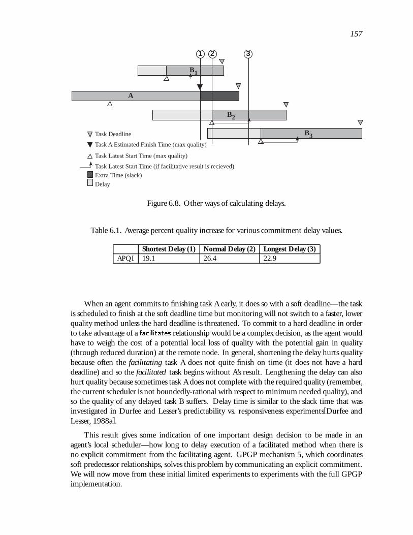
157

B1

A

B3

B2

Task Deadline

Task A Estimated Finish Time (max quality)

Task Latest Start Time (max quality)

Extra Time (slack)

Delay

Task Latest Start Time (if facilitative result is recieved)

1 32

Figure 6.8. Other ways of calculating delays.

Table 6.1. Average percent quality increase for various commitment delay values.

Shortest Delay (1) Normal Delay (2) Longest Delay (3)APQI 19.1 26.4 22.9

When an agent commits to finishing task A early, it does so with a soft deadline—the taskis scheduled to finish at the soft deadline time but monitoring will not switch to a faster, lowerquality method unless the hard deadline is threatened. To commit to a hard deadline in orderto take advantage of a facilitates relationship would be a complex decision, as the agent wouldhave to weigh the cost of a potential local loss of quality with the potential gain in quality(through reduced duration) at the remote node. In general, shortening the delay hurts qualitybecause often the facilitating task A does not quite finish on time (it does not have a harddeadline) and so the facilitated task begins without A’s result. Lengthening the delay can alsohurt quality because sometimes task A does not complete with the required quality (remember,the current scheduler is not boundedly-rational with respect to minimum needed quality), andso the quality of any delayed task B suffers. Delay time is similar to the slack time that wasinvestigated in Durfee and Lesser’s predictability vs. responsiveness experiments[Durfee andLesser, 1988a].

This result gives some indication of one important design decision to be made in anagent’s local scheduler—how long to delay execution of a facilitated method when there isno explicit commitment from the facilitating agent. GPGP mechanism 5, which coordinatessoft predecessor relationships, solves this problem by communicating an explicit commitment.We will now move from these initial limited experiments to experiments with the full GPGPimplementation.

158

6.2 GPGP Simulation: Issues

Our model of an abstract task environment, used in the rest of this chapter, has tenparameters; Table 6.2 lists them and the values used in the experiments described in the nexttwo sections. These were discussed in some detail in Section 3.6.2. Figure 6.12 shows twosmall task groups generated with the parameters from Table 6.6, which are similar.

Table 6.2. Environmental Parameters used to generate the random episodes

Parameter Values (facilitation exps.) Values (clustering exps.)Mean Branching factor (Poisson) 1 1Mean Depth (Poisson) 3 3Mean Duration (exponential) 10 (1 10 100)Redundant Method QAF Max MaxNumber of task groups 2 (1 5 10)Task QAF distribution (20%/80% min/max) (50%/50% min/max)

(100%/0% min/max)Hard CR distribution (10%/90% enables/none) (0%/100% enables/none)

(50%/50% enables/none)Soft CR distribution (80%/10%/10% facilitates/hinders/none) (0%/10%/90% facilitates/hinders/none)

(50%/10%/40% facilitates/hinders/none)Chance of overlaps (binomial) 10% (0% 50% 100%)Facilitation Strength .1 .5 .9 .5

The primary sources of overhead associated with the coordination mechanisms includeaction executions (communication and information gathering), calls to the local scheduler,and any algorithmic overhead associated with the mechanism itself. Table 6.3 summarizes thetotal amount of overhead from each source for each coordination mechanism setting and thecoordination substrate. L represents the length of processing (time before termination), and dis a general density measure of coordination relationships. We believe that all of these amountscan be derived from the environmental parameters in Table 6.2, they can also be measuredexperimentally. Interactions between the presence of coordination mechanisms and thesequantities include: the number of methods or tasks inE, which depends on the non-local viewmechanism; the number of coordination relationships jCRj or the subsets RCR (redundantcoordination relationships), HPCR (hard predecessor coordination relationships), SPCR(soft predecessor coordination relationships), which depends on the number of tasks andmethods as well; and the number of commitments jCj, which depends on each of the threemechanisms that makes commitments.

6.3 General Performance Issues

Another question is how the performance of a fully configured system compares withoptimal performance. While we have no optimal parallel scheduler with which to compareourselves, we do have a single agent optimal scheduler and a centralized, heuristic parallelscheduler that takes the single-agent optimal schedule as its starting point.

We examined the general performance of the most complex (all mechanisms in place) andleast complex (all mechanisms off) members of the GPGP family in comparison to each other,

159

Table 6.3. Overhead associated with individual mechanisms at each parameter setting

Mechanism setting Communications Information Gathering Scheduler Other Overheadsubstrate 0 E+idle L O(LC)nlv none 0 0 0 0

some O(dP) Edetect-CRs 0 O(T 2 E)all O(P) Edetect-CRs 0 O(T 2 E)

comm min O(C) 0 0 O(C)TG O(C +E) 0 0 O(C +E)all O(M 2 E) 0 0 O(M 2 E)

redundant on O(RCR) 0 0 O(RCR � S +CR)hard on O(HPCR) 0 O(HPCR) O(HPCR � S +CR)soft on O(SPCR) 0 O(SPCR) O(SPCR � S +CR)

and in comparison to a centralized scheduler reference implementation (as an upper bound).We looked at performance measures such as the total final quality achieved by the system,the amount of work done, the number of deadlines missed, and the termination time. Thecentralized schedule reference system is not an appropriate solution to the general coordinationproblem, even for cooperative groups of agents, for several reasons:

� The centralized scheduling agent becomes a possible single point of failure that can causethe entire system to fail (unlike the decentralized GPGP system).

� The centralized scheduling agent requires a complete, global view of the episode—a viewthat we mentioned earlier is not always easy to achieve. We do not account for any costsin building such a global view in the reference implementation (viewing it as an upperbound on performance). We do not allow dynamic changes in the episodic task structure(which might require rescheduling).

� The centralized reference scheduler uses an optimal single-agent schedule as a startingpoint. The problem of scheduling actions in even fairly simple task structures is NP-complete, and the optimal scheduler’s performance grows exponentially worse with thenumber of methods to be scheduled. Since the centralized reference scheduler has aglobal view and schedules all actions at all agents, the size of the centralized problemalways grows faster than the size of the scheduling problems at GPGP agents with onlypartial views and heuristic schedulers.

We conducted 300 paired response experiments, using the three algorithms. “Balanced”refers to all mechanisms being on, with partial non-local views and communication ofcommitted results and completed task groups. “Simple” refers to all mechanisms being off,with no non-local view and broadcast communication of all results. “Parallel” refers to thecentralized reference scheduler that uses a heuristic parallelization of an optimal single agentschedule using a complete global view. The experiments were based on the same environmentalparameters as the facilitation experiments (Table 6.2). There are several important things tonote about this class of environments:

160

� The size of the episodes was kept artificially small so that the centralized referencescheduler could find an optimal schedule in a reasonable amount of run time.

� The experiments had very low (10%)numbers of enables relationships and a low (20%)number of MIN quality accrual functions because they penalize the simple algorithm—we demonstrate this in Section 6.8. High numbers of enables constraints tend to hurtthe uncoordinated agents because they have no mechanism for handling precedenceexcept ‘wait until enabled’. If there is also a low overlap percentage, the uncoordinatedagents, who do not exchange non-local views, will not be able to apply even this simplerule because they will not even know of the existence of the enabling method.

� Deadline pressure was also kept low (it also makes the simple algorithm perform badly).

In our experiments, the centralized parallel scheduler outperformed our distributed, GPGPagents 57% of the time (36% no difference, 7% distributed was better) using the total finalquality as the only criterion. The GPGP agents produced 85% of the quality that the centralizedparallel scheduler did, on average. These results need to be understood in the proper context—the centralized scheduler takes much more processing time that the distributed scheduler andcan not be scaled up to larger numbers of methods or task groups. The centralized scheduleralso starts with a global view of the entire episode. Table 6.4 shows the results for all fourmeasured criteria by summarizing within-block (paired-response) comparisons. 4 For totalfinal quality and number of deadlines missed, “better” simply refers to an episode where thealgorithm in question had a greater total final quality or missed fewer deadlines, respectively.With respect to method execution time (a measure of system load) and termination time,“better” refers to the fact that one algorithm produced both a higher quality and missed fewerdeadlines than the other algorithm, or if the two algorithms were the same, then the betteralgorithm had a lower total method execution time (lower load) or terminated sooner.5

We also looked at performance without any of the mechanisms; on the same 300 episodesthe GPGP agents produced on average 1.14 times the final quality of the uncoordinated agents.Coordinated agents (“balanced”) execute far fewer methods because of their ability to avoidredundancy. The redundant execution of methods proves a much more hindering element tothe uncoordinated agents when acting under severe time pressure [Decker, 1994b]. Table 6.5summarizes the results.

6.4 Taking Advantage of a Coordination Relationship: When to Add a New Mechanism

A practical question to ask is simply whether the addition of a particular mechanism willbenefit performance for the system of agents. Here we give an example with respect to thesoft coordination mechanism, which will make commitments to facilitation relationships. Weran 234 randomly generated episodes (generated with the environmental parameters shown inTable 6.2) with four agents both with and without the soft coordination mechanism. Becausethe variance between these randomly generated episodes is so great, we took advantage of the

4Communication can not be measured fairly because the centralized parallel scheduler had instantaneouscommunication to all agents and instantaneous access to all results.

5Termination within two time units was considered “the same” because the “balanced” algorithm has a fixed2-unit startup cost. The average task duration is 10 time units.

161

Table 6.4. Performance comparison: Centralized Parallel Scheduler vs. Balanced GPGPCoordination and Decentralized DTT Scheduler

Parallel better Balanced Better Same Significant?Total Final Quality 57% 7% 36% yes

Method Execution Time 80% 7% 13% yesDeadlines Missed 1% 1% 98% no

Termination Time 67% 15% 18% yes

Table 6.5. Performance comparison: Simple GPGP Coordination vs. Balanced GPGPCoordination

Simple better Balanced Better Same Significant?Total Final Quality 8% 21% 71% yes

Method Execution Time 12% 72% 16% yesDeadlines Missed 0% 4% 96% yes

Termination Time 9% 58% 33% yes

paired response nature of the data to run a non-parametric Wilcoxon matched-pairs signed-ranks test [Daniel, 1978]. This test is easy to compute and makes very few assumptions—primarily that the variables are interval-valued and comparable within each block of pairedresponses. For each of the 234 blocks we calculated the difference in the total final qualityachieved by each group of agents and excluded the blocks where there was no difference, leaving102 blocks. We then replace the differences with the ranks of their absolute values, and thenreplace the signs on the ranks. Finally we sum the positive and negative ranks separately. Astandardized Z score is then calculated. A small value of Z means that there was not muchconsistent variation, while a large value is unlikely to occur unless one treatment consistentlyoutperformed the other. In our experiment, the null hypothesis is that the system with thesoft coordination mechanism did the same as the one without it, and our alternative is thatthe system with the soft coordination mechanism did better (in terms of total final quality).The result here was Z = �6:9, which is highly significant, and allows us to reject the nullhypothesis that the mechanism did not have an effect.

6.5 Different Family Members for Different Environments

In this section I will show a particular example of how different family members do betterand worse in different environments. I will concentrate on two distinct family members—the‘modular agent’ archetype (all CR modules on, non-local views, communicate commitmentsand completed task groups), and the ‘simple agent’ (no CR modules on, no non-local views,broadcast all completed methods). The environmental parameter we will vary (derived fromthe screening data collected in Section 6.8) is QAF-min, the percentage of tasks that have min as

162

their quality accumulation function (‘AND’ semantics). Our hypothesis was that the modularagents would do better than the simple agents as QAF-min increased (as more tasks needed tobe done). We ran 250 paired-response experiments at 5 levels of QAF-min (0, 0.25, 0.5, 0.75,1.0) with enables-probability varying also at the same 5 levels, no time pressure, overlaps of 0.5,5 task groups, and 4 agents per run. The performance (in terms of total final quality) of the twocoordination styles was significantly different by the Wilcoxon matched-pairs signed-ranks test(199 different pairs, Z = �3:27, p � 0:0005). More interestingly, we can see the differencein performance widening with the value of QAF-min. Figure 6.9 shows the probability of onecoordination style or the other doing better (calculated simply from the frequencies) plottedverses the value of QAF-min. This allows you to see graphically the difference in the stylesas QAF-min changes. Figure 6.10 shows the same information as probability partitions foreach of the three possible outcomes as QAF-min changes, determined by (exploratory) logisticregression. The hash marks on the right edge of each box show the base partition valuescomputed from all the data while ignoring the value of QAF-min.

0.1

0.2

0.3

0.4

0.5

0.6

0.7

Modular Agent

Simple Agent

0.0 0.1 0.2 0.3 0.4 0.5 0.6 0.7 0.8 0.9 1.0

Qaf-Min

Prob

abili

ty o

f doi

ng b

ette

r

Figure 6.9. Plot of the probability of the modular or simple coordination styles doing betterthan the other (total final quality) verses the probability of task quality accumulation beingMIN (AND-semantics)

163

0

0.25

0.5

0.75

1

0.0 0.1 0.2 0.3 0.4 0.5 0.6 0.7 0.8 0.9 1.0

Qaf-Min

Worse

Same

Better

Pro

babi

lity

Par

titi

on (

Sim

ple

Age

nt)

0

0.25

0.5

0.75

1

0.0 0.1 0.2 0.3 0.4 0.5 0.6 0.7 0.8 0.9 1.0

Qaf-Min

Pro

babi

lity

Par

titi

on (

Mod

ular

Age

nt)

Better

Same

Worse

Figure 6.10. Probability partitions for one style doing the same, better, or worse than the othergiven the value of QAF-min.

6.6 Meta-level Communication: Return to Load Balancing through Dynamic Reorganiza-tion

Another question we have examined is the effect of task structure variance on theperformance of load balancing algorithms. This work is a logical follow-on to the analysis ofstatic, dynamic, and negotiated reorganization detailed in the last chapter. A static organizationdivides the load up a priori—in the case below, by randomly assigning redundant tasks to agents.A one-shot dynamic reorganization, like that analyzed in Chapter 4, assigns redundant tasks onthe basis of the expected load on other agents. A meta-level communication (MLC) reorganizationassigns redundant tasks on the basis of actual information about the particular problem-solvingepisode at hand. Because it requires extra communication, the MLC reorganization is moreexpensive, but the extra information pays off as the variance in static agent loads grows.6

A MLC coordination mechanism (mechanism 6) can be implemented in GPGP. Manysuch implementations are possible; the one that we chose works by altering the way redundantcommitments are handled. When a commitment is sent to another agent, it is modified toinclude the current load of the agent making the commitment (to be precise, the amount of workfor the agent in the current schedule). Whenever a decision about redundant commitmentsneed to be made at another agent (in mechanisms 3, 4, and 5—simple redundancy, hard, andsoft successor relationship handling) the load of the agents with the redundant commitmentsare taken into account at the point where ties would have been broken randomly. The agentwith the lowest load keeps the commitment instead. If the loads are equal, the tie is brokenrandomly as before.

The effect of this mechanism on the general GPGP environments when agents use thedefault Design-To-Time scheduler is minimal. The heuristics used by the DTT scheduler arefocused at providing the highest possible total final quality for the agent without violatingdeadlines—this is not the same as terminating quickly, and the scheduler has no heuristics to

6See also Mirchandaney’s [Mirchandaney et al., 1989] paper on the effects of delays on load balancing insimple distributed systems.

164

prefer earlier termination times (nor, frankly, should it have them). In a randomly-generatedtask environment, where the methods are assigned to agents randomly (and therefore, somewhatevenly) there is rarely any significant change in termination time.

However, if you recall one of our results from Chapter 4, you will remember that MLCcoordination is most useful in environments with high variance in the task structures presentedto agents. We can look at our experiments in this light, by calculating an endogenous inputvariable for each run that represents the amount of variance in redundant tasks (the ones thatwould potentially be eligible for a load-balancing mechanism decision). Figure 6.11 shows howthe probability of terminating more quickly with the MLC load balancing algorithm grows asthe standard deviation in the total durations of redundant tasks at each agent grows.

Prob

abili

ty T

erm

inat

ion

is B

ette

r w

/ Lo

ad B

alan

cing

0

0.25

0.5

0.75

1

0 10 20 30 40 50

Initial STD of Redundant Tasks

Expected probability

Actual probability

Figure 6.11. Probability that MLC load balancing will terminate more quickly than static loadbalancing, fitted using a loglinear model from actual TÆMS simulation data.

6.7 Computational Organizational Design

Another application for the use of TÆMS as a modeling tool for asking and answeringquestions about organizational design, as was discussed in Chapter 3. In this final section wereplicate a classic computational organization design study done by Burton and Obel ([Burtonand Obel, 1984]) using GPGP agents.

165

6.7.1 Burton and Obel Experiments

In this section we will consider the use of TÆMS as a simulator to explore hypothesesabout the interactions between environmental and agent-structural characteristics. We useas an example a question explored by Burton and Obel: is there a significant difference inperformance due to either the choice of organizational structure or the decomposability oftechnology7?

We equate a technology with a TÆMS task structure, instead of a linear program. Taskstructures allow us to use a clear interval measure for decomposability, namely the probabilityof a task interrelationship (in this example enables, facilitates, and overlaps). We define a nearlydecomposable task structure to have a base probability of 0.2 for these three coordinationrelationships and a less decomposable task structure to have a base probability of 0.8 (seeFigure 6.12). We will continue in this example to look at purely computational task structures,although the use of physical resources can also be represented (see [Decker and Lesser, 1993e]).

Burton and Obel were exploring the difference in M-form (multidivisional) and U-form(unitary—functional) hierarchical structures; we will analyze the GPGP family of team-orientedcoordination algorithms. For our structural variable we will vary the communication ofnon-local views (GPGP Module 1). Informally, we will be contrasting the situation whereeach agent makes commitments and communicates results based only on local information(no non-local view) with one where the agents freely share task structure information withone another across coordination relationships (partial non-local view). Figure 6.13 shows anexample—note that in neither case does the agent have the global view of Figure 6.12.

Burton and Obel used a profitability index as their performance measure, derived fromthe percentage of optimal profit achieved. In general, the scheduling an arbitrary TÆMS taskstructure is an NP-hard problem and so we do not have access to optimal solutions. Insteadwe compare performance directly on four scales: the number of communication actions, theamount of time spent executing methods, the final quality achieved, and the terminationtime. Simulation runs for each of the four combinations of non-local view policy and levelof task decomposability were done in matched sets—the randomly generated episode was thesame for each combination with the exception of more coordination relationships (includingmore overlapping methods) being added in the less decomposable task structures. FollowingBurton and Obel, we used the non-parametric Friedman two-way analysis of variance byranks test for our hypotheses. The assumptions of this test are that each block (in our case,randomly generated episode) is independent of the others and that each block contains matchedobservations that may be ranked with respect to one another. The null hypothesis is that thepopulations within each block are identical.

We generated 40 random episodes of a single task group, each episode was replicated for thefour combinations in each block. We used teams consisting of 5 agents; the other parametersused in generating the task structures are summarized in Table 6.6 and a typical randomlygenerated structure is shown in Figure 6.12. Figure 6.13 shows the difference in the localview of one agent with and without creating partial non-local views. We first tested two majorhypotheses:

7Technology is used here in the management science sense of “the physical method by which resources areconverted into products or services” or a “means for doing work” [Burton and Obel, 1984, Scott, 1987].

166

Table 6.6. Parameters used to generate the 40 random episodes

Parameter ValueMean Branching factor (Poisson) 1Mean Depth (Poisson) 3Mean Duration (exponential) 10Redundant Method QAF MaxNumber of task groups 1Task QAF distribution (50% min) (50% max)Decomposition parameter p = 0.2 or 0.8Hard CR distribution (p enables) ((1-p) none)Soft CR distribution (p facilitates) (10% hinders)

((.9-p) none)Chance of overlaps (binomial) p

Tmin

task with quality accrual function min

subtask relationship

enables relationship

method (executable task)

facilitates relationship

agent

Tmin

Tmax

Tmax

Tmax

Tmax

Tmax

Tmax

A B C D E

A B C D E

B C D E

Tmin

Tmax

Tmax

Tmax

Tmax

Tmax

Tmax

E

A C E

B E

More Decomposable (p=0.2)Less Decomposable (p=0.8)

Figure 6.12. Example of a randomly generated objective task structure, generated with theparameters in the previous table.

167

Hypothesis 1: There is no difference in performance between agents with a partial non-local viewand those without. For the communication and method execution performance measures,we reject the null hypothesis at the 0.001 level. We cannot reject the null hypothesisthat there is no difference in final quality and termination time. Teams of computationalagents that exchange information about their private, local views consistently exchangemore messages (in this experiment, a mean increase of 7 messages) but do less work (here,a mean decrease of 20 time units of work, probably due mostly to avoiding redundancy).

Hypothesis 2: There is no difference in performance due to the level of decomposability of technology.For the communication and method execution performance measures, we reject thenull hypothesis at the 0.001 level. We cannot reject the null hypothesis that thereis no difference in final quality and termination time. Teams of computational agents,regardless of their policy on the exchange of private, local information communicate moremessages (in this experiment, a mean increase of 47 messages) and do more work (here, amean increase of 24 time units) when faced with less decomposable computational taskstructures (technology).

Again following Burton and Obel, we next test for interaction effects between non-local view policy and level of technology decomposability by calculating the differences inperformance at each level of decomposability, and then testing across non-local view policy.This test was not significant. To reiterate, based on the experimental results in this section itseems that TÆMS has potential for use in computational organization theory, though this is outof the scope of this dissertation.

Tmin

Tmax

Tmax

Tmax

Tmax

Tmax

A C E

Partial Non-local View at Agent A (p=0.2) No Non-Local View at Agent A (p=0.2)

Tmin

Tmax

Tmax

A

Figure 6.13. Example of the local view at Agent A when the team shares private informationto create a partial non-local view and when it does not.

6.8 Exploring the Family Performance Space

Finally, we looked at the multidimensional performance space for the family of coordinationalgorithms over four different performance measures. At the most abstract level, each of thefive mechanisms are parameterized independently (the first two have three possible settingsand the last three can be ‘in’ or ‘out’) for a total of 72 possible coordination algorithms.

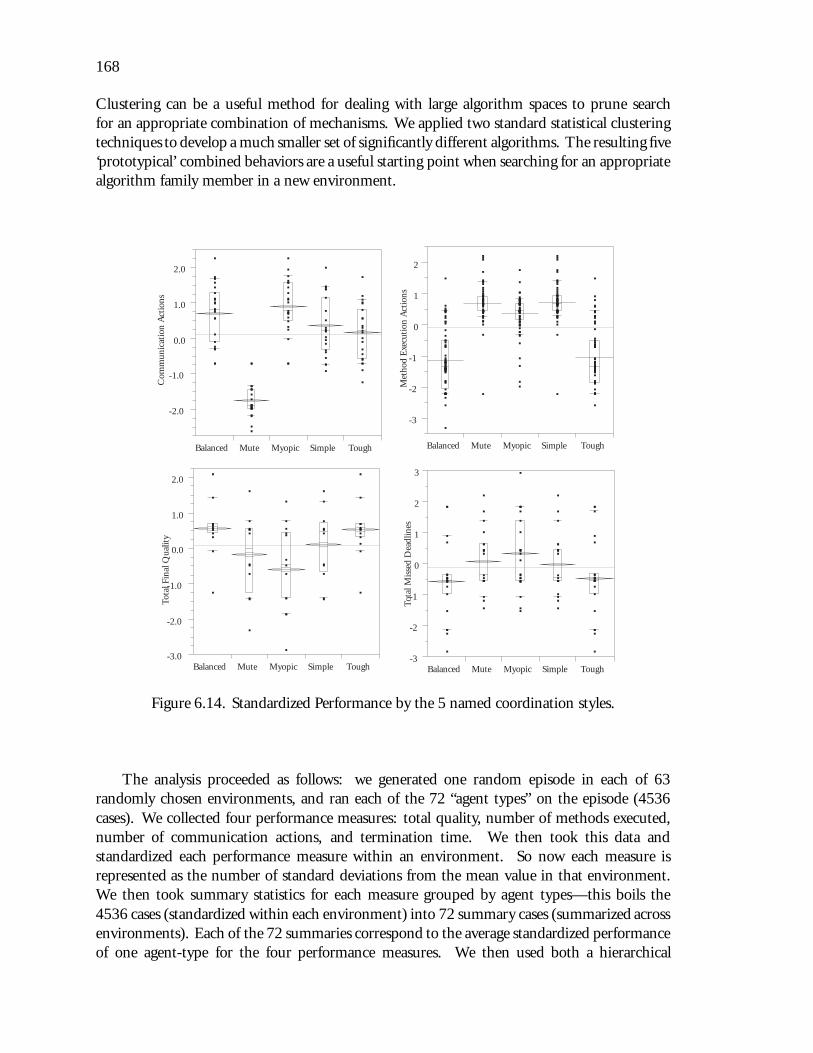
168

Clustering can be a useful method for dealing with large algorithm spaces to prune searchfor an appropriate combination of mechanisms. We applied two standard statistical clusteringtechniques to develop a much smaller set of significantly different algorithms. The resulting five‘prototypical’ combined behaviors are a useful starting point when searching for an appropriatealgorithm family member in a new environment.

-2.0

-1.0

0.0

1.0

2.0

Balanced Mute Myopic Simple Tough

-3

-2

-1

0

1

2

Balanced Mute Myopic Simple Tough

Com

mun

icat

ion

Act

ions

Met

hod

Exe

cuti

on A

ctio

ns

-3.0

-2.0

-1.0

0.0

1.0

2.0

Balanced Mute Myopic Simple Tough-3

-2

-1

0

1

2

3

Balanced Mute Myopic Simple Tough

Tota

l Fin

al Q

ualit

y

Tota

l Mis

sed

Dea

dlin

es

Figure 6.14. Standardized Performance by the 5 named coordination styles.

The analysis proceeded as follows: we generated one random episode in each of 63randomly chosen environments, and ran each of the 72 “agent types” on the episode (4536cases). We collected four performance measures: total quality, number of methods executed,number of communication actions, and termination time. We then took this data andstandardized each performance measure within an environment. So now each measure isrepresented as the number of standard deviations from the mean value in that environment.We then took summary statistics for each measure grouped by agent types—this boils the4536 cases (standardized within each environment) into 72 summary cases (summarized acrossenvironments). Each of the 72 summaries correspond to the average standardized performanceof one agent-type for the four performance measures. We then used both a hierarchical

169

clustering algorithm (SYSTAT JOIN with ‘complete linkage’8) to produce the following generalprototypical agent classes (we chose one representative algorithm in each class):

Simple: No commitments or non-local view, just broadcasts results.

Myopic: All commitment mechanisms on, but no non-local view.

Balanced: All mechanisms on.

Tough-guy: Agent that makes no soft commitments.

Mute: No communication whatsoever9

Figure 6.14 shows the values of several typical performance measures for only the fivenamed types. Performance measures were standardized within each episode, (i.e_across all 72types). Shown for each are the means and 10, 25, 50, 75, and 90 percent quantiles. All agents’performances are significantly different by Tukey Kramer HSD except for: Method Execution(Simple vs. Mute), Total final quality (Balanced vs. Tough), Deadlines missed (simple vs.mute) and (balanced vs. tough).

We are also analyzing the effect of environmental characteristics on agent performance.Figure 6.15 shows an example of the effect of the a priori amount of overlap on the numberof method execution actions for the five named agent types. Note again that the balanced andtough agents do significantly less work when there is a lot of overlap (as would be expected).The performance of the tough and balanced agents is similar because (from Table 6.2) onlyhalf the experiments had any facilitation, and when it was present was only at 50% power.

A linear clustering algorithm, SYSTAT KMEANS, produces a similar result as hierarchicalclustering, and also produces the mean value of each performance measure for each group, soyou can in fact see that the non-communicating agents have a high negative mean "number-of-communications" (-1.16–remember these were averaged from standardized scores) but executemore methods on average and produce less final quality. They also terminate slightly quickerthan average. Our "Balanced" group, in comparison, communicates a little more than average,executes many fewer methods (-1.29—way out on the edge of this statistic), returns better-than-average quality and about average termination time. This is reasonable, as ‘avoiding redundantwork’ and other work-reducing ideas are a key feature of the GPGP algorithm. For examplepurposes, complete KMEANS output for 48 of the agent types10 is listed in Tables 6.7 and 6.8.Each of the 48 agent types is summarized by a alphabetic genotype. The first letter is ‘H’ ifmechanism 5 (Hard relationships) is on and ‘–’ if it is off. The second letter is ‘S’ if mechanism4 (Soft relationships) is on and ‘–’ if it is off. The third letter is ‘R’ if mechanism 3 (simpleRedundancy) is on and ‘–’ if it is off. The fourth letter indicates the state of mechanism 1(non-local views): ‘s’ for some and ‘n’ for none. The fifth and final letter indicates the stateof mechanism 2 (result communication): ‘A’ for all, ‘C’ for commitments only, and ‘T’ forcommitments + task groups. Note that the KMEANS clustering groups ‘simple’ and ‘myopic’together, and puts ‘– – – s T’ and ‘– – – s C’ in a different cluster. I chose to keep ‘simple’

8Distances are calculated between the farthest points in each cluster. Other distance measures (Euclidean,centroid, or Pearson correlation) gave similar results.

9This algorithm makes no commitments (mechanisms 3, 4, and 5 off ) and communicates (mechanism 2)only ‘satisfied commitments’—therefore it sends no communications ever!.

10Agents with mechanism 1 (non-local views) set to ‘all’ were accidentally omitted.

170

Met

hod

Exe

cuti

on A

ctio

ns

-3

-2

-1

0

1

2

-0.1 0.1 0.3 0.5 0.7 0.9 1.1Overlap

Balanced

Tough

Myopic

MuteSimple

Figure 6.15. The effect of overlaps in the task environment on the standardized methodexecution performance by the 5 named coordination styles (smoothed splines fit to the means).

and ‘myopic’ separated because they are different in an interesting way (‘myopic’ has everymechanism on except for the exchange of non-local views), whereas the two others are basicallyas uninteresting as ‘Mute’ except that they exchange non-local views which fool them into doingno work and then waiting around forever (until the deadline) for the results to be sent (whichor course never happens since only committed results are communicated and no commitmentsare made).

6.9 Summary

In this chapter I described several experiments using TÆMS and the GPGP algorithm.This chapter differs from Chapter 4 in that the focus here is on examining the performanceof computer programs, rather than the abstract mathematical analysis of a problem that usescomputer programs only for verification. First this chapter described some simple experimentsshowing the effect of facilitation power and likelihood on agents; the rest of the chapter focusedon Generalized Partial Global Planning.

The chapter showed how to decide if the addition of a new GPGP mechanism was useful.It showed the general performance of two GPGP family algorithms compared to a centralizedparallel reference algorithm; GPGP with all mechanisms ‘on’ produces 85% of the quality of thecentralized reference scheduler implementation in a random environment. Such performanceis reasonable and we feel could be made better by developing better local scheduling algorithmsand new coordination mechanisms.

This chapter contained a demonstration of how a feature of the task environment (theprobability of task quality accumulation being MAX) can cause different GPGP family membersto be preferred. This chapter also discussed a sixth mechanism, a load balancing mechanism

171

Table 6.7. Complete KMEANS linear clustering output for all 72 agent types, first threeclusters. All performance parameters were standardized within blocks.

CLUSTER NUMBER: 1Members Statistics

CASE DISTANCE VARIABLE MINIMUM MEAN MAXIMUM ST.DEV.SIMPLE - - - nA 0.30 Comm 0.06 0.55 1.20 0.30

- - RnA 0.17 MEA -0.34 0.29 0.57 0.28-S-nA 0.17 TFQ -0.24 0.09 0.42 0.23-SRnA 0.25 Term -0.35 -0.02 0.14 0.14H- - nA 0.16H-RnA 0.22HS-nA 0.22HSRnA 0.36- - - sA 0.16-S-sA 0.30

H- - sA 0.26HS-sA 0.36- - RnT 0.32-SRnT 0.14H-RnT 0.13

Myopic HSRnT 0.20HSRnC 0.24

CLUSTER NUMBER: 2Members Statistics

CASE DISTANCE VARIABLE MINIMUM MEAN MAXIMUM ST.DEV.- - - sT 0.32 Comm -1.26 -1.03 -0.80 0.23- - - sC 0.32 MEA -0.02 -0.02 -0.02 0.00

TFQ -0.37 -0.37 -0.37 0.00Term 1.27 1.88 2.48 0.60

CLUSTER NUMBER: 3Members Statistics

CASE DISTANCE VARIABLE MINIMUM MEAN MAXIMUM ST.DEV.-S-nT 0.26 Comm -0.94 -0.49 -0.07 0.28

H- - nT 0.15 MEA -0.34 -0.01 0.56 0.31HS-nT 0.35 TFQ -0.53 0.03 0.63 0.42-S-sT 0.21 Term -0.29 -0.05 0.15 0.16

Tough H- - sT 0.27HS-sT 0.41-SRnC 0.32H-RnC 0.27HS-nC 0.34-S-sC 0.30

H- - sC 0.35HS-sC 0.36

172

Table 6.8. Complete KMEANS linear clustering output for all 72 agent types, continued. Allperformance parameters were standardized within blocks.

CLUSTER NUMBER: 4Members Statistics

CASE DISTANCE VARIABLE MINIMUM MEAN MAXIMUM ST.DEV.- - RsA 0.21 Comm -0.37 0.45 1.27 0.48-SRsA 0.27 MEA -1.49 -1.29 -1.12 0.14H-RsA 0.36 TFQ -0.35 0.25 0.63 0.40HSRsA 0.47 Term -0.22 -0.01 0.20 0.16- - RsT 0.40-SRsT 0.21H-RsT 0.21

Balanced HSRsT 0.27- - RsC 0.52-SRsC 0.31H-RsC 0.31HSRsC 0.22

CLUSTER NUMBER: 5Members Statistics

CASE DISTANCE VARIABLE MINIMUM MEAN MAXIMUM ST.DEV.- - - nT 0.18 Comm -1.68 -1.16 -0.75 0.33

Mute - - - nC 0.27 MEA 0.15 0.43 0.57 0.17- - RnC 0.24 TFQ -0.31 -0.25 -0.20 0.03-S-nC 0.07 Term -0.35 -0.19 0.03 0.13

H- - nC 0.16

that communicates meta-level information, and showed that it was somewhat more useful whenthe variance in duration of the agents’ overlapping tasks was high. This section thus ties-inback to the discussion at the end of Chapter 4 on the usefulness of meta-level communication(in this case, the transmission of local load information) when the inter-episode variance (inthis case, in the initial agent loads) is high.

The chapter also presented a version of Burton and Obel’s task decomposability experimentthat used GPGP agent teams instead of hierarchical organizational structures. As in Burton andObel’s result, we showed that both the task structure decomposability and the organizationalstructure (in our case, the state of the non-local view communication mechanism) have asignificant effect.

Finally, we gave a sense of the performance space of the 5 broadly-parameterized mech-anisms using a clustering technique. Clustering can be a useful method for dealing withlarge algorithm spaces to prune search for an appropriate combination of mechanisms. Suchmethods may also lead to ways to learn situation-specific knowledge about the application ofcertain mechanisms in certain situations (perhaps using case-based reasoning techniques).

173

Some of the things that are in this chapter that I talked about in Chapter 1 include doingpaired-response comparisons of different coordination algorithms in Section 6.2, doing ablationstudies of the addition/deletion of mechanisms and its effect on performance (Section 6.8) andexamining computerized methods for organizational design (Section 6.7). Finally, this chapterdescribed several sets of experiments that dealt with the performance of the GPGP mechanismsin different environments, using a real implementation (running in Common Lisp on multipleplatforms, and being used by more than one person). The implementation uses as submodulesa real implementation of Garvey’s Design-To-Time real-time scheduler [Garvey and Lesser,1994].

We believe that GPGP can become a reusable, domain-independent basis for multi-agentcoordination when used in conjunction with a library of coordination mechanisms and alearning mechanism. We intend to develop such a library of reusable coordination mechanisms.For example, mechanisms that work from the successors of hard and soft relationships insteadof the predecessors, negotiation mechanisms, mechanisms for behavior such as contracting, ormechanisms that can be used by self-motivated agents in non-cooperative environments. Manyof these mechanisms can be built on the existing work of other DAI researchers. Future work willalso examine expanding the parameterization of the mechanisms and using machine learningtechniques to choose the appropriate parameter values (i.e., learning the best mechanism setfor an environment). Finally, we are also beginning work on using the GPGP approach inapplications ranging from providing human coordination assistance to distributed informationgathering. This will be discussed in the next chapter in the Future Work section. Thenext chapter, which is the final chapter, will summarize the previous chapters and discuss theextremely interesting new areas of research to which this dissertation leads us.

174

C H A P T E R 7

CONCLUSIONS

From decentralization we get responsibility, development of personnel, decisions closeto the facts, flexibility—in short, all of the qualities necessary for an organization toadapt to new conditions. From coordination we get efficiencies and economies. It mustbe apparent that coordinated decentralization is not an easy concept to apply.

— Alfred P. Sloan, Jr., My Years with General Motors

Coordination is the process of managing interdependencies between activities [Maloneand Crowston, 1991]. This dissertation focused on the problem of representing theseinterdependencies in a formal, domain-independent way.

This dissertation demonstrated a framework that can be used to specify the task structureof any computational environment, called TÆMS. It then instantiated an existing methodology(MAD: Modeling, Analysis and Design [Cohen, 1991]) using this framework to analyze aparticular computational environment (Distributed Sensor Networks) and predict and verify theperformance of two simple coordination algorithms in that environment. Finally, we designeda family of generic coordination mechanisms for cooperative, soft real-time computational taskenvironments and demonstrated their performance and why a family of mechanisms is neededinstead of a single static algorithm.

7.1 Summary: Representing Task Environments

This dissertation was about how to represent coordination problems in a formal, domain-independent way. Such a representation should abstract out the details of the domain, andleave the basic coordination problem—the choice and temporal ordering of possible actions.Our solution to this problem was a framework called TÆMS (Task Analysis, EnvironmentModeling, and Simulation), which can be used to specify, reason about, analyze, and simulateany computational environment. The unique features of TÆMS include:

� The explicit, quantitative representation of task interrelationships. Both hard andsoft, positive and negative relationships can be represented. When relationships in theenvironment extend between tasks being worked on by separate agents, we often call themcoordination relationships, because they can be used to design and analyze coordinationmechanisms. We demonstrated the usefulness of coordination relationships in creatingcoordination mechanisms in Chapters 5 and 6. We gave definitions for fifteen usefulrelationships in Chapter 3. The set of relationships is extensible.

� The representation of structures at multiple levels of abstraction. The lowest level ofabstraction is called an executable method. A method represents a schedulable entity,such as a blackboard knowledge source instance, a chunk of code and its input data,

176

or a totally-ordered plan that has been recalled and instantiated for a task. A methodcan also be an instance of a human activity at some useful level of detail, for example,“take an X-ray of patient 1’s left foot”. A task group contains all tasks that have explicitcomputational interrelationships.

� The representation of structure from three different viewpoints. The first view is agenerative model of the problem solving episodes in an environment—a statistical viewof the task structures. The second view is an objective view of the actual, real, instantiatedtask structures that are present in an episode. The third view is the subjective view thatthe agents have of the objective task structures.

� TÆMS makes very few assumptions about what an ‘agent’ is. TÆMS defines an agent asa locus of subjective belief (or state) and action (executing methods, communicating,and acquiring subjective information about the current problem solving episode). Thisis important because the study of principled agent construction is a very active area. Byseparating the notion of agency from the model of task environments, we do not haveto subscribe to particular agent architectures (which one would assume will be adaptedto the task environment at hand), and we may ask questions about the inherent socialnature of the task environment at hand (allowing that the concept of society may arisebefore the concept of individual agents [Gasser, 1991]). Such a conception is uniqueamong computational approaches.

� TÆMS allows us to clearly specify concepts and subproblems important to multi-agent andAI scheduling approaches. For example, we discussed the difference between “anytime”and “design-to-time” algorithms using TÆMSin Chapter 3. Garvey [Garvey et al., 1993]uses TÆMS to define the concept of a minimum duration schedule that achieves maximumquality.

� This dissertation is about computational task environments, where methods are thingslike blackboard knowledge source instantiations. However, we also described extensionsof TÆMS to represent physical resource constraints.

Along with its formal definition, we also described a simulator for TÆMS written in portableCLOS (the Common Lisp Object System) and using CLIP[Westbrook et al., 1994] for datacollection.

We validated this framework by building a detailed model of the complex DSN en-vironment of the Distributed Vehicle Monitoring Testbed (DVMT). Our model includedfeatures that represent approximate processing, faulty sensors and other noise sources, lowquality solution errors, sensor configuration artifacts, and vehicle tracking phenomena such astraining and ghost tracks. Simulations of simplified DSN models showed many of the samecharacteristics as were seen in the DVMT [Durfee et al., 1987]. We also described models ofmany other environments: hospital patient scheduling, a post office problem, airport resourcemanagement, multi-agent Internet information gathering, and pilot’s associate. Finally, wevalidated our framework by allowing others to use it in their work—on design-to-timescheduling, on parallel scheduling, on the diagnosis of errors in local area networks, andin the future to model software engineering activities.

177

7.2 Summary: Analyzing a Distributed Sensor Network Environment

The second major result reported here was a detailed analysis of a simplified DSNenvironment. The methodology behind this analysis is an instantiation of the MAD (Modeling,Analysis, and Design) methodology [Cohen, 1991], with TÆMS providing the modeling andsimulation components. This part of the dissertation returns to the work of Durfee, Lesser,and Corkill [Durfee et al., 1987] that showed that no single coordination algorithm uniformlyoutperformed the others. This dissertation explained that result, and went on to predict theperformance effects of changing:

� the number of agents

� the physical organization of agents (i.e., the range of their sensors and how much thesensed regions overlap)

� the average number of vehicles in an episode

� the agents’ coordination algorithm

� the relative cost of communication and computation

These predictions were verified by simulation.For example, in Chapter 4 we derived and verified an expression for the time of termination

of a set of agents in any arbitrary simple DSN environment that has a static physical organizationand coordination algorithm. We used this expression (Eq. 4.9) as a predictor by combining itwith the probabilities for the values of S and N . We verified this model using the simulationcomponent of TÆMS.

Our analysis explained another observation that has been made about the DVMT—thatthe extra overhead of meta-level communication is not always balanced by better performance.This work represents the first detailed analysis of a DSN, and the first quantitative, statisticalanalysis of any Distributed AI system outside Sen’s work on distributed meeting scheduling fortwo agents [Sen and Durfee, 1994].

7.3 Summary: Designing a Family of Coordination Mechanisms

The third major result reported here was the design and evaluation of a family ofcoordination mechanisms for cooperative computational task environments. We called thecollection of resulting algorithms the Generalized Partial Global Planning (GPGP) familyof algorithms. GPGP both generalizes and extends Durfee’s Partial Global Planning (PGP)algorithm [Durfee and Lesser, 1991]. Our approach has several unique features:

� Each mechanism is defined as a response to certain features in the current subjectivetask environment. Each mechanism can be removed entirely, or parameterized so thatit is only active for some portion of an episode. New mechanisms can be easily defined.An initial set of five mechanisms was examined and we added a sixth (a simple loadbalancing mechanism).

� GPGP works in conjunction with an existing agent architecture and local scheduler. Theexperimental results reported here were achieved using a ‘design-to-time’ soft real-timelocal scheduler developed by Garvey [Garvey and Lesser, 1993].

178

� GPGP, unlike PGP, is not tied to a single domain.

� GPGP allows more agent heterogeneity than PGP with respect to agent capabilities.

� GPGP mechanisms in general exchange less information than the PGP algorithm,and the information that GPGP mechanisms exchange can be at different levels ofabstraction. PGP agents generally communicate complete schedules at a single, fixedlevel of abstraction. GPGP mechanisms communicate scheduling commitments toparticular tasks, at any convenient level of abstraction.

The fact that most of the GPGP coordination mechanisms use commitments to other agentsas local scheduling constraints is the reason that the GPGP family of algorithms requirescooperative agents. Nothing in TÆMS the underlying task structure representation, requiresagents to be cooperative, antagonistic, or simply self-motivated. We could develop or co-opt mechanisms to enforce the keeping of agent commitments (for instance, as contracts[Sandholm, 1993]) in non-cooperative environments.

In verifying the GPGP family of algorithms, we first showed that they duplicate andsubsume the behaviors of the PGP algorithm. We then looked at several other issues:General Performance: We examined the general performance of the most complex (all mech-

anisms in place) and least complex (all mechanisms off) members of the GPGP familyin comparison to each other, and in comparison to a centralized scheduler referenceimplementation (as an upper bound). We looked at performance measures such as thetotal final quality achieved by the system, the amount of work done, the number ofdeadlines missed, and the termination time. The centralized schedule reference systemis not an appropriate solution to the general coordination problem, even for cooperativegroups of agents, for several reasons:

� The centralized scheduling agent becomes a possible single point of failure that cancause the entire system to fail (unlike the decentralized GPGP system).

� The centralized scheduling agent requires a complete, global view of the episode—aview that we mentioned earlier is not always easy to achieve. We do not account forany costs in building such a global view in the reference implementation (viewingit as an upper bound on performance). We do not allow dynamic changes in theepisodic task structure (which might require rescheduling).

� The centralized reference scheduler uses an optimal single-agent schedule as astarting point. Since the problem of scheduling actions in even fairly simple taskstructures is NP-complete, the optimal scheduler’s performance grows exponentiallyworse with the number of methods to be scheduled. Since the centralized referencescheduler has a global view and schedules all actions at all agents, the size of thecentralized problem always grows faster than the size of the scheduling problemsat GPGP agents with only partial views. The size of the episodes was kept smallso that the centralized reference scheduler could find an optimal schedule in areasonable amount of run time.

The performance of set of agents using all of the currently defined GPGP coordinationmechanisms is good in comparison to the centralized reference system—GPGP agentsproduce on average 85% of the quality of the centralized upper bound reference solution,and do not miss any more deadlines.

179

Adding a Mechanism: We demonstrated that the addition of a particular mechanism canimprove the system performance.

Family Design Space: We demonstrated the range of performance exhibited by differentmembers of the GPGP algorithm family, obtained by simple parameterization of theindividual coordination mechanisms.

Different Environments: We showed that different environments require different familymembers.

Load Balancing: We demonstrated how a new sixth mechanism, a load balancing mechanism,can be defined and integrated. We used this mechanism to show that the costs of usingthis mechanism are better balanced by performance improvements precisely when thereis a large variance in the amount of work each agent would do by default. This resultagrees with similar results in the distributed processing community on decentralized loadbalancing [Need a citation here].

Computational Organization Design: We recreated a set of experiments done by Burton andObel [Burton and Obel, 1984] that examined the effects of technical interdependenciesand organizational structure on the performance. GPGP team-oriented coordinationmechanisms were used to define the organizational (team) structure, and TÆMS taskstructures defined the problem (as opposed to Burton and Obel’s linear programs). Wereached the same conclusions as Burton and Obel (that both do have an effect), andargued that one future application for TÆMS is as a tool for computational organizationdesign.

TÆMS, as a framework to represent coordination problems in a formal, domain-independentway, is unlike any existing representation that is focussed on coordination issues. As a problemrepresentation, it is richer and more expressive than game theory or team theory representations.For example, a typical game or team theory problem statement is concerned with a singledecision; a typical TÆMS objective problem solving episode represents the possible outcomesof many sequences of choices (interrelated with one another). TÆMS can represent a gametheoretic problem, and we could boil down a single decision made by an agent faced with aTÆMS task structure into a game theoretic problem (if there were no uncertainty involved—seeChapter 2). Because TÆMS is more expressive, we can use it to operationalize some of therich but informal concepts of organizational science (such as decomposability in Section 6.7).Another difference between TÆMS and traditional distributed computing task representationsis that TÆMS indicates that not all tasks in an episode need to be done.

To put the second part of this dissertation in context, the analysis of a simple distributedsensor network presented here is the first formal quantitative analysis of a DSN or DAI system,other than Sen’s analysis of a two-agent distributed meeting scheduling system (developed at thesame time) [Sen and Durfee, 1994]. Our analysis of a DSN system answers several questions,and explains phenomena observed in the work with the Distributed Vehicle Monitoring Testbed(DVMT) such as why different algorithms perform differently in different situations. The workdescribed here moves beyond anecdotal data to design rules for DSN systems.

GPGP, the last major contribution of this dissertation, extends Durfee’s work on PartialGlobal Planning by being domain independent, adding time deadlines, allowing the agentsto be more heterogeneous, requiring less communication, and allowing communication at

180

multiple levels of detail. GPGP is a cooperative approach, and thus is different from algorithmsthat assume the agents act in rational self-interest only. For example, agents usually makedecisions with much less a priori knowledge of the other agents’ utilities than competitivegame theory approaches. However, agents using GPGP mechanisms still make decisions ina boundedly rational way—choosing from among schedules in an attempt to maximize thesystem-wide utility given whatever subjective information they have.

7.4 Limitations of this work

The work described here is of course not without limitations. The framework forrepresenting the task structure of any computational environment, /tems (Chapter 3), hasseveral limitations. Some of these are currently being addressed in follow-up work. /tems/describes an environment from three different viewpoints—the generative viewpoint of howindividual episodes come about, the objective viewpoint of the actual structure of an episode,and the subjective viewpoint of the agents themselves. This dissertation concentrates on theobjective viewpoint. It does not deal with the various representations of uncertainty that mightbe in an agent’s subjective view—we are currently working on this aspect. The generativemodels in this dissertation are constructed from a statistical viewpoint—an episode can becharacterized by the values of several random variables. While this is far better than using a setof single-instance examples, it may not be appropriate for dynamic environments, where thetask structure itself is changing dramatically over time. More complex models of generationmay be needed. For example, generation might be modeled by a set of meta-agents.

The idea of the task structure changing dramatically over time is also often importantin modeling human organizations. Human organizations often face external forces that canreshape the very structure of their environment. For example, the way the government canenact new laws that affect certain businesses. Factors that influence organizational behavioror measures of organizational performance might change out from under the organization(which then must adapt). As we discussed in Section 2.2.2, these responses need not always begenuine, they might only be symbolic. Nothing in this dissertation deals with such immediate,unbounded uncertainty, or how and organization might decide between a symbolic or genuineresponse.1 Furthermore, we have not discussed periodic or other cyclic, recurring task structureshere, except as a source of future work.

Our results on the analysis of a simple Distributed Sensor Network in Chapter 4 are limitedonly by the simplicity of the domain. Some extensions, such as having more than one vehicletype, would be fairly simple. Other extensions, such as having the vehicles move in patterns,would invalidate parts of the model (but not all of it). For example, if vehicles tended to stayon certain paths (roads or underwater rifts), then this information could be used to give newa priori distributions of agent loads in an episode; the average load for each agent might verywell be unequal. However, the work calculations in that chapter would still hold. The mainlimitation of the DSN analysis is that it cannot yet be automated.

The final major contribution, the Generalized Partial Global Planning family of algorithms(Chapter 5), has several limitations. First of all, the existing set of mechanisms can only be

1As a first approximation, one might adopt a multiple-criteria definition for quality, including an “externalvisibility” attribute. Symbolic responses (modeled as alternative methods of low cost, high external visibility, butlow true quality) might then be chosen under stressful situations.

181

used by cooperative agents. Self-interested or antagonistic agents could take advantage ofthe commitment mechanism (for example) to cheat other agents. There is a great deal ofwork on mechanisms that can avoid this problem (at some cost of overhead). For example,commitments can be viewed as contracts and enforced by a third party. In some environments,repetitive episodes can bring about a rational self-interested decision to cooperate, such asAxelrod’s tit-for-tat strategy in the Prisoner’s Dilemma. The second limitation is that there arecurrently only 6 mechanisms, which will not suffice for arbitrary environments. The existingmechanisms do not, for example, allow for hierarchical organizations. Finally, there is as yetno learning component, so the designer is responsible for choosing when a mechanism shouldbe used. We believe this limitation can also be overcome, as we will discuss in the section onFuture Work (Section 7.5, next).

7.5 Future Work

The work described in this dissertation leads directly to several applications, extensions,and new directions.

The subjective level. We present the TÆMS’ subjective level in this dissertation, but we do notuse it to any great extent except in a few examples. Work has already begun on describingthe various types of subjective uncertainties that can be present in task environmentssuch as DRESUN. Previous DTT scheduling work has already considered some simpletypes of subjective uncertainty, such as the duration and actual quality of methods.

Other subjective level extensions include the indication of methods that provide onlysubjective information (i.e., provide better estimates for the duration of methods). Thescheduler will then have to decide when to schedule these meta-level actions rather thandomain-level method executions.

Resources. It is exciting to us that the basic TÆMS mechanisms can handle the representationof physical resources as described in Section 3.4.5. However, the notation is a bitponderous and could be improved with some ‘syntactic sugar’ (as Steele would say). Forexample, since all resource relationships come in pairs, we could define them by a singledouble relationship (that would have the same semantics as the pair of relationshipsused now). More importantly, we can begin to develop or adapt local schedulers toschedule task structures with resources (both the Spring scheduler [Cheng et al., 1988,Shen et al., 1993] and Hildum’s DSS scheduler [Hildum, 1994] are examples of suchschedulers). Finally, we can begin to develop new coordination mechanisms to handlehigh-level, flexible resource usage. Some ideas about this can be found in Sycara’s andNieman’s papers [Neiman et al., 1994, Sycara et al., 1991].

Hard real-time. We hint in Section 5.7 about using GPGP in concert with a true hard real-timeoperating system (i.e. Spring). Part of doing this involves the interface between the DTTscheduler and the Spring scheduler, part involves GPGP. TÆMS methods would probablybe equivalent to Spring task groups. The resulting larger system would not be hardreal-time, but only time-cognizant. It would be interesting to look at what a Springguarantee means at a distance (i.e., wrapped in a GPGP commitment). An example ofsuch a system might be a football team (with soft-real-time interaction between playsand hard real-time during the plays).

182

Load balancing. The demonstration in Section 6.6 hardly does this subject justice. A consid-erable amount of effort could be put into developing a more comprehensive set of GPGPload balancing mechanisms. The analysis of such mechanisms could be attempted bysimplifying the environment as we did in Chapter 4 and by making assumptions aboutcertain properties of the local scheduler with respect to termination.

Learning. As we described at the start and end of Chapter 5, GPGP is a family of algorithms—each of the five mechanisms described here are parameterized independently (the firsttwo have three possible settings and the last three can be in or out) for a total of 72combinations. More mechanisms such as the load balancing mechanism can been addedto expand the family, but the family can also be enlarged by making each mechanismmore situation-specific. For example, mechanisms can have their parameters set by amapping from dynamic meta-level measurements such as an agent’s load or the amountof real-time pressure. Mechanisms can be ‘in’ or ‘out’ for individual classes of taskgroups, or tasks, or even specific coordination relationships, that re-occur in particularenvironments. The cross product of these dynamic environmental cues provides a largebut easily enumerated space of potential coordination responses that are amenable tothe adaptation of the coordination mechanisms over time by standard machine learningtechniques or case-based reasoning approaches.

GPGP as DAI infrastructure. GPGP could be developed as a modular, extendible, portableset of coordination modules that could be linked into existing applications to providecoordination assistance. The application would supply the task structure and codestubs for resolving and discovering coordination relationships, and possibly also a localscheduler. Mechanisms could be chosen by the programmer or by learning mechanismssuch as those just described.

Societies creating agents. Throughout this dissertation, we have focused on the environmentaffecting agents. In reality, the environment and agents co-create one another (e.g.,[Latour, 1987]). The only AI work ever to even being to address this question is Gasserand Ishida’s work on self-organizing rule-based systems [Gasser and Ishida, 1991]. Gasserhas been talking for years about the chicken-and-egg problem of agents and the society(e.g., [Gasser, 1991]), but most computer scientists cannot conceive of anything exceptsocieties created out of their agents, and never visa versa. The Gasser and Ishida paperpresents a model where the problem exists and creates the agents—reversing the normalindividualistic process. If there is a problem with this work, it is that the environmentis only a simple set of rules. A clear forward direction is to use TÆMS task structuresinstead of rules to specify the task environment. What kind of rules would be needed forthe formation of individuals (agents) from this beginning? When would individuals bereabsorbed? Would different environments cause the creation of different organizationalstructures? We assume that they would. This is related to the next point.

Computational organization design (COD). Future work will include the analysis of moretraditional hierarchical organization forms. The addition of the concept of ‘organiza-tional role’ can be accomplished through the use of non-local commitments (and theiraccompanying expectations). In its simplest sense, agent A’s organizational role is a setof continuing non-local commitments to certain classes of tasks. By making continuous

183

commitments agents can avoid communicating about every episode anew—assumingthe future structures are somewhat predictable. This reasoning leads naturally to learningorganizational roles and to open systems concepts of temporarily settled questions (thecurrent set of continuous commitments) and algorithms to re-open and re-settle thesequestions as the task environment changes. The development of such algorithms canthen lead to exploring conceptions of agents as nothing more than convenient bundlesof organizational roles [Gerson, 1976, Gasser et al., 1989], and to when and whyorganizations do not act like ‘big agents’ [Allison, 1971]. We will also allow the expansionof commitments to meta-level roles (i.e., commitments to the coordination parameters ineffect for certain classes of tasks). Related applications fall under the popular buzzwordsBusiness Process Re-Engineering.

Computational organization theory. Related to COD is the idea of producing computationalversions of traditional organization theories. For example, Masuch and Huang areformalizing J.D. Thompson’s Organizations in Action using a multi-agent action logic[Masuch and Huang, 1994]. The book Computational Organization Theory[Carley andPrietula, 1994] is all about mathematical, logical, and computational approaches; a newbook by the same editors will be about purely computational models (including the onepresented in this dissertation). K. Crowston [personal communication] has talked aboutproducing an entire book of computational versions of famous organizational theories,complete with the programs, for students to experiment with. Williamson’s TransactionCosts Economics [Williamson, 1975] would be an example theory that could be modeledin TÆMS.

Negotiating Agents. A direct consequence of heterogeneous, dynamic, and real-time agents isthe need for negotiation to solve conflicts. Even with a known global decision evaluationfunction, conflicting decisions of equal global value may have very different local valueto the agents. Often the character of an early partial solution will have an impact onwhat style of coordination is needed. For example, if early partial results show poordata and low beliefs, the coordination mechanism may want to encourage redundantderivations of results in areas shared by more than one agent, or the parallel derivationof a result by two agents using different algorithms. The Pilot’s Associate scenario inSection 3.6.3.4 occurs in too short a time-frame to allow negotiation between the agents,but other Pilot’s Associate scenarios might profitably use negotiation techniques2.

The PGP mechanism uses a shared global plan evaluation function that is parameterized.One extension is to allow the parameters (such as redundancy and reliability) to varyduring problem solving. A negotiation facility could be developed to allow agents tousefully alter the global (or perhaps only semi-local — we are interested in agents thatmay develop only a partial view of what other agents are working on) decision criteria.Where the PGP mechanisms exchanged all local information, our extensions would allowfor a multi-stage process [Conry et al., 1991] where agents would communicate only theinformation believed relevant to the issue at hand. Agents could ask for more contextual

2For example, a sensor may overheat and be shut down by the system status module, even though it is aprojected resource requirement for some tactical situation. The tactical planner and system status may negotiateover the amount of time that the damaged sensor can be used if the situation arises.

184

information when it is needed to resolve a conflict between agents. Agents would notautomatically acquire information from other agents performing non-related problemsolving activities. Negotiation can interact with sophisticated real-time local schedulersthat have the capability to analyze potential future schedules.

GPGP in multi-agent systems. This is a whole area of mechanisms that could be incorporatedfrom the rational, selfish agent community. New mechanisms would need to bedeveloped to deal with the possibility of lying or other potentially ‘uncooperative’behavior. Results from the game theoretic DAI community could be adapted fairlyeasily.

Dynamic Episodes. Up to this point, we have focused on the interrelationships and theuncertainty arising directly from the generative model of the environment, but wewould also like to explore the uncertainty and variance arising from the difference in theobjective and subjective models. Different relationships between these models will leadto different organizational structures. For example, in the case of uncertainty arisingfrom the generative model of an environment, we showed that the wide variance inperformance of a system of agents with static organizations in different episodes led tothe use of meta-level communication to reorganize the agents to adapt to the particularepisode at hand [Decker and Lesser, 1993c]. We are also looking to expand the TÆMS

conception of environments to encompass more dynamic situations: another importantsource of environmental uncertainty. For example, in the Tower of Babel problem [Ishida,1992], agents try to pile numbered blocks into a tower in numerical order. When manyagents try to solve this problem without centralized coordination, they tend to bottleneckaround the tower itself, bumping into one another. Ishida solves this problem by dividingthe agents into two groups: one to collect blocks and bring them near (but not too near)the tower, and one group to stack the tower. From our point of view, the task structureat low levels is changing rapidly, and no agent can (or needs to) keep track of all thechanges in relationships between agent and block positions. The rapid change in theenvironment means that agents’ subjective views are always out of date. By dividing theagents into two groups, the bottleneck resource is controlled by organization—removingit from the uncertainties facing the agents. Stacking agents know there are not enough ofthem to saturate the bottleneck, and other agents no longer use the resource at all. Theuncertainty is still there, but it no longer has an impact on the agents’ decision-makingprocess.

Coordination assistance for mixed human and computational agent systems. The operationalvision of the ARPA/Rome Labs Planning Initiative (ARPI) is one of a network ofworkstations that enable concurrent and distributed assessment, plan generation, andanalysis. It envisions that groups of humans and computational ‘agents’ will cooperativelycreate, resource, evaluate, execute, and monitor crisis management or manufacturingplans. Both problems and opportunities arise from a truly distributed and cooperativeenvironment. A possible area of future work would be the development of support toolsfor distributed, cooperative work by groups of human and computational agents, basedon TÆMS and GPGP.

In ARPA’s Air Campaign Planning domain, for example, the development of objectives,target analyses, and situational analyses (e.g. identification of centers-of-gravity (COGs))

185

are mixed initiative processes that can take place concurrently, and are carried outby the JFACC (Joint Forces Air Component Commander) and his staff (intelligence,operations, logistics, weather, etc.). As the planner makes decisions to focus on certainenemy vulnerabilities, he creates (concurrent) taskings for intelligence and other staffmembers or computational agents; as the staff uncovers certain information, that sameinformation may impact back on the main planning task (revealing logistical, intelligence,or other problems with certain targets). This pattern of interrelated task structures thatare partially shared by multiple agents with mixed initiative tasking appears in manymilitary and commercial environments (transportation planning, target assignment,hospital scheduling, manufacturing scheduling, coordinating large software developmentefforts). These interrelationships provide not only potential problems to avoid (such asforgetting a required task) but also opportunities to take advantage of (such as doing atask needed by more than one other agent first, or doing a favor for another agent).

In general, each person and computational agent involved in such distributed cooperativework has a set of initially unrelated tasks before them that currently need to be done(identifying targets in several areas, collecting intelligence on each of several disparatetargets, etc.). One possible way to assist users in task selection is by developingsomething like a User Coordination Assistant Agent (UCAA) that keeps track of aworkstation user’s current agenda of tasks and presents a possible schedule (ordering)of these tasks according to user- and domain-directed preferences. Such an agenda isnot developed in isolation, but rather through a distributed coordination process usingmultiple coordination mechanisms triggered by the coordination relationships between thetask structures of the different agents involved. A similar Agent Coordination Module(ACM) could be developed for purely computational agents. The ACM would provideagenda management services for coordinating computational agents in the context ofuser task-order preferences.

Such a set of tools will allow the development of systems that can truly support commandand control planning. Such planning will involve both people at multiple workstationsand computational agent assistants. The tools will help to manage and organize theworkloads of both these types of agents. Certain tasks will be dependent on othertasks and be time critical, and such information for differentiating tasks could belost in critical situations if only ad hoc coordinating mechanisms are used. Moreinformation than simply task assignments and task coordination relationships is usefulto communicate. For example, users and computational agents can request possible duedates for potential tasks before assignment (allowing both better time estimates and loadbalancing) and request commitments to complete certain time-critical tasks (in effect,supporting inter-agent negotiation protocols). Our approach of tying coordinationmechanisms to the particular kinds of coordination relationships that exist in a particulartask environment provides for a reusable tool foundation (the UCAA and its interactivehuman interface, the ACM and its interface to a computational agent) and a customizableset of coordination mechanisms for a particular application environment (since nosingle coordination mechanism would be useful across environments with different taskcoordination relationships).

186

Coordination and scheduling assistance for ARCADIA, a software engineering environment.Arguments similar to those in the last item apply to other domains, such as the concurrentengineering of products where designers, engineers, sales/marketing representatives andmanufacturing staffers work together to develop a new product or an extension of an oldproduct. We have already been exploring the use of our technology in the representationand management of large software engineering projects to help schedule tasks beingperformed by many different programmers using many different resources. Part ofthe ARCADIA [Kadia, 1992, Taylor et al., 1988] environment is directly concernedwith representing and tracking the state of: software development processes (includinginterrelationships), the products being produced, and the resources available. Thisinformation can be used by a UCAA-like application that can provide scheduling andcoordination facilities to ARCADIA users. The most unique feature of this domain isthe presence of high levels of uncertainty in task durations (compared to manufacturingdomains).

Multi-agent distributed information gathering. Distributed information gathering applica-tions using the Internet might look something like the following using the technologydeveloped in this thesis: The original user query would be transformed into set of agents,each with their own plans for gathering information, where some plan elements mustdeal with the coordination of activities and construction of the final query response.Agents could be assigned to concurrently pursue different sources to answer differentaspects of the query or to make use of alternative types of sources (e.g., text vs. images)to generate a more comprehensive answer. The agents would proceed to work in adistributed, asynchronous fashion, but there may need to be coordination among theagents. For example, the results of work by one agent may suggest the need for some ofthe existing agents to gather additional information from their sources or use alternativesources, or it might suggest the need for additional agents. The agents must also dealwith uncertainties about the availability of sources and the workload associated with thesources, which may require a new division of tasks among the agents.

REFERENCES

[Adler et al., 1989] M.R. Adler, A.B. Davis, R. Weihmayer, and R.W. Worrest. Conflictresolution strategies for nonhierarchical distributed agents. In L. Gasser and M. N. Huhns,editors, Distributed Artificial Intelligence, Vol. II, pages 139–162. Pitman Publishing Ltd.,1989. Also COINS Technical Report 88-89, University of Massachusetts, 1988.

[Agre, 1991] Philip E. Agre. Title undecided. To be published by Cambridge University Press.Position paper presented at AAAI Fall Symposium on Knowledge and Action at Social andOrganizational Levels, 1991.

[Allison, 1971] Graham T. Allison. Essence of Decision: Explaining the Cuban Missle Crisis.Little, Brown and Company, Boston, 1971.

[Anderton, 1994] D.L. Anderton. Anderton questions for decker’s defense. Private Commu-nication., 1994.

[Axelrod, 1984] R. Axelrod. The Evolution of Cooperation. Basic Books, New York, 1984.

[Blau and Schwartz, 1984] P.M. Blau and J.E. Schwartz. Crosscutting Social Circles: Testing aMacrostructural Theory of Group Relationships. Academic Press, New York, 1984.

[Boddy and Dean, 1989] Mark Boddy and Thomas Dean. Solving time-dependent planningproblems. In Proceedings of the Eleventh International Joint Conference on Artificial Intelligence,pages 979–984, Detroit, August 1989.

[Bond and Gasser, 1988] Alan H. Bond and Les Gasser. An analysis of problems and researchin DAI. In Alan H. Bond and Les Gasser, editors, Readings in Distributed ArtificialIntelligence, pages 3–35. Morgan Kaufmann, 1988.

[Bonissone and Decker, 1986] Piero P. Bonissone and Keith S. Decker. Selecting uncertaintycalculi and granularity: An experiment in trading-off precision and complexity. In L. N.Kanal and J. F. Lemmer, editors, Uncertainty in Artificial Intelligence. North Holland, 1986.

[Broverman et al., 1987] C. A. Broverman, K. E. Huff, and V. R. Lesser. The role of planrecognition in design of an intelligent user interface. In Proceedings of the IEEE Systems,Man, and Cybernetics Conference, pages 863–868, Atlanta, Georgia, 1987.

[Burrell et al., 1994] G. Burrell, M. Reed, M. Alverson, M. Calas, and L. Smircich. WhyOrganization? why now? Organization, 1(1):5–17, 1994.

[Burt, 1982] R.S. Burt. Toward a structural theory of action : network models of social structure,perception, and action. Quantitative studies in social relations. Academic Press, New York,1982.

[Burton and Obel, 1984] Richard M. Burton and Børge Obel. Designing Efficient Organiza-tions: Modelling and Experimentation. North Holland, Amsterdam, 1984.

[Cammarata et al., 1983] Stephanie Cammarata, David McArthur, and Randall Steeb. Strate-gies of cooperation in distributed problem solving. In Proceedings of the Eighth InternationalJoint Conference on Artificial Intelligence, pages 767–770, Karlsruhe, Germany, August 1983.

188

[Carley and Prietula, 1994] K.M. Carley and M.J. Prietula, editors. Computational Organiza-tion Theory. Lawrence Erlbaum Associates, 1994.

[Carver et al., 1991] Norman Carver, Zarko Cvetanovic, and Victor Lesser. Sophisticatedcooperation in FA/C distributed problem solving systems. In Proceedings of the NinthNational Conference on Artificial Intelligence, pages 191–198, Anaheim, July 1991.

[Carver, 1994] N. Carver. A note on multi-agent information retrieval. Private Communica-tion., 1994.

[Castelfranchi, 1993] C. Castelfranchi. Commitments:from individual intentions to groupsand organizations. In Michael Prietula, editor, AI and theories of groups & organizations:Conceptual and Empirical Research. AAAI Workshop, 1993. Working Notes.

[Chambers et al., 1984] F.B. Chambers, D.A. Duce, and G.P. Jones, editors. DistributedComputing, volume 20 of APIC Studies in Data Processing. Academic Press, London, 1984.

[Chandrasekaran, 1981] B. Chandrasekaran. Natural and social system metaphors for dis-tributed problem solving: Introduction to the issue. IEEE Transactions on Systems, Man,and Cybernetics, 11(1):1–5, January 1981.

[Cheng et al., 1986] S. Cheng, J.A. Stankovic, and K. Ramamritham. Dynamic schedulingof groups of tasks with precedence constraints in distributed hard real-time systems. InReal-time Systems Symposium, December 1986.

[Cheng et al., 1988] S. Cheng, J. Stankovic, and K. Ramamritham. Scheduling algorithmsfor hard real-time systems. In Hard Real-Time Systems. IEEE Press, 1988.

[Chisholm, 1989] Donald Chisholm. Coordination Without Hierarchy: Informal Structures inMultiorganizational Systems. University of California Press, Berkeley, 1989.

[Cohen and Levesque, 1990] Philip R. Cohen and Hector J. Levesque. Intention is choicewith commitment. Artificial Intelligence, 42(3):213–261, 1990.

[Cohen et al., 1989] Paul Cohen, Michael Greenberg, David Hart, and Adele Howe. Trialby fire: Understanding the design requirements for agents in complex environments. AIMagazine, 10(3):33–48, Fall 1989. Also COINS-TR-89-61.

[Cohen, 1991] Paul R. Cohen. A survey of the Eighth National Conference on ArtificialIntelligence: Pulling together or pulling apart? AI Magazine, 12(1):16–41, Spring 1991.

[Cohen, 1992] Paul R. Cohen. Tactics for generalization. Course notes for ExperimentalDesign in AI, 1992.

[Conry et al., 1991] S. E. Conry, K. Kuwabara, V. R. Lesser, and R. A. Meyer. Multistagenegotiation for distributed constraint satisfaction. IEEE Transactions on Systems, Man, andCybernetics, 21(6), November 1991.

[Corkill and Lesser, 1983] Daniel D. Corkill and Victor R. Lesser. The use of meta-levelcontrol for coordination in a distributed problem solving network. In Proceedings of theEighth International Joint Conference on Artificial Intelligence, pages 748–755, Karlsruhe,Germany, August 1983.

[Corkill, 1979] Daniel D. Corkill. Hierarchical planning in a distributed environment. InProceedings of the Sixth International Joint Conference on Artificial Intelligence, pages 168–175,Cambridge, 1979. Also COINS TR–79–13.

189

[Crowston, 1994] Kevin Crowston. Coordinating restaurant service: An analysis of TGIFriday’s process. Presentation given at the TIMS/ORSA Workshop on Mathematical andComputational Organization Theory, April 1994. Crowston is a professor at the Universityof Michigan School of Business.

[Daniel, 1978] W. W. Daniel. Applied Nonparametric Statistics. Houghton-Mifflin, Boston,1978.

[Davis and Smith, 1983] R. Davis and R. G. Smith. Negotiation as a metaphor for distributedproblem solving. Artificial Intelligence, 20(1):63–109, January 1983.

[Dean and Wellman, 1991] T. L. Dean and M. P Wellman. Planning and Control. MorganKaufman Publishers, San Mateo, California, 1991.

[Dean, 1987] Thomas Dean. Planning, execution, and control. In Proceedings of the DARPAKnowledge-based Planning Workshop, December 1987.

[Decker and Lesser, 1990] Keith S. Decker and Victor R. Lesser. Extending the partial globalplanning framework for cooperative distributed problem solving network control. InProceedings of the Workshop on Innovative Approaches to Planning, Scheduling and Control,pages 396–408, San Diego, November 1990. Morgan Kaufmann. Also COINS TR-90-81.

[Decker and Lesser, 1992] Keith S. Decker and Victor R. Lesser. Generalizing the partialglobal planning algorithm. International Journal of Intelligent and Cooperative InformationSystems, 1(2):319–346, June 1992.

[Decker and Lesser, 1993a] Keith S. Decker and Victor R. Lesser. Analyzing a quantitativecoordination relationship. Group Decision and Negotiation, 2(3):195–217, 1993.

[Decker and Lesser, 1993b] Keith S. Decker and Victor R. Lesser. An approach to analyzingthe need for meta-level communication. In Proceedings of the Thirteenth International JointConference on Artificial Intelligence, pages 360–366, Chambery, France, August 1993.

[Decker and Lesser, 1993c] Keith S. Decker and Victor R. Lesser. A one-shot dynamiccoordination algorithm for distributed sensor networks. In Proceedings of the EleventhNational Conference on Artificial Intelligence, pages 210–216, Washington, July 1993.

[Decker and Lesser, 1993d] Keith S. Decker and Victor R. Lesser. Quantitative modeling ofcomplex computational task environments. In Proceedings of the Eleventh National Conferenceon Artificial Intelligence, pages 217–224, Washington, July 1993.

[Decker and Lesser, 1993e] Keith S. Decker and Victor R. Lesser. Quantitative modeling ofcomplex environments. International Journal of Intelligent Systems in Accounting, Finance,and Management, 2(4):215–234, December 1993. Special issue on “Mathematical andComputational Models of Organizations: Models and Characteristics of Agent Behavior”.

[Decker et al., 1990] Keith S. Decker, Victor R. Lesser, and Robert C. Whitehair. Extendinga blackboard architecture for approximate processing. The Journal of Real-Time Systems,2(1/2):47–79, 1990.

[Decker et al., 1991] Keith S. Decker, Alan J. Garvey, Marty A. Humphrey, and Victor R.Lesser. Effects of parallelism on blackboard system scheduling. In Proceedings of the TwelfthInternational Joint Conference on Artificial Intelligence, pages 15–21, Sydney, Australia, August1991. Extended version to appear in the International Journal of Pattern Recognition andArtificial Intelligence 7(2) 1993.

190

[Decker et al., 1992] Keith Decker, Alan Garvey, Marty Humphrey, and Victor Lesser. Ablackboard system for real-time control of approximate processing. In Proceedings of the25th Hawaii International Conference on System Sciences, January 1992. Extended version toappear in the International Journal of Pattern Recognition and Artificial Intelligence 7(2)1993.

[Decker et al., 1993a] Keith S. Decker, Alan J. Garvey, Marty A. Humphrey, and Victor R.Lesser. Control heuristics for scheduling in a parallel blackboard system. InternationalJournal of Pattern Recognition and Artificial Intelligence, 7(2):243–264, 1993.

[Decker et al., 1993b] Keith S. Decker, Alan J. Garvey, Marty A. Humphrey, and Victor R.Lesser. A real-time control architecture for an approximate processing blackboard system.International Journal of Pattern Recognition and Artificial Intelligence, 7(2):265–284, 1993.

[Decker, 1987] Keith S. Decker. Distributed problem solving: A survey. IEEE Transactionson Systems, Man, and Cybernetics, 17(5):729–740, September 1987.

[Decker, 1994a] Keith S. Decker. Distributed artificial intelligence testbeds. In G. O’Hareand N. Jennings, editors, Foundations of Distributed Artificial Intelligence, chapter 3. WileyInter-Science, 1994. Forthcoming.

[Decker, 1994b] Keith S. Decker. Environment Centered Analysis and Design of CoordinationMechanisms. PhD thesis, University of Massachusetts, 1994.

[Decker, 1994c] Keith S. Decker. Tæms: A framework for analysis and design of coordinationmechanisms. In G. O’Hare and N. Jennings, editors, Foundations of Distributed ArtificialIntelligence, chapter 16. Wiley Inter-Science, 1994. Forthcoming.

[Dubois and Prade, 1984] D. Dubois and H. Prade. Criteria aggregation and ranking ofalternatives in the framework of fuzzy set theory. In H.J. Zimmermen, L. A. Zadeh, andB.R. Gains, editors, TIMS/Studies in Management Science, volume 20, pages 209–240.Elsevier Science Publishers, 1984.

[Durfee and Lesser, 1987] Edmund H. Durfee and Victor R. Lesser. Using partial globalplans to coordinate distributed problem solvers. In Proceedings of the Tenth InternationalJoint Conference on Artificial Intelligence, August 1987.

[Durfee and Lesser, 1988a] E. Durfee and V. Lesser. Predictability vs. responsiveness: Co-ordinating problem solvers in dynamic domains. In Proceedings of the Seventh NationalConference on Artificial Intelligence, pages 66–71, St. Paul, Minnesota, August 1988.

[Durfee and Lesser, 1988b] Edmund H. Durfee and Victor R. Lesser. Incremental planning tocontrol a time-constrained, blackboard-based problem solver. IEEE Transactions on Aerospaceand Electronic Systems, 24(5):647–662, September 1988.

[Durfee and Lesser, 1989] Edmund H. Durfee and Victor R. Lesser. Negotiating taskdecomposition and allocation using partial global planning. In L. Gasser and M. N.Huhns, editors, Distributed Artificial Intelligence, Vol. II. Pitman Publishing Ltd., 1989.

[Durfee and Lesser, 1991] E.H. Durfee and V.R. Lesser. Partial global planning: A coordina-tion framework for distributed hypothesis formation. IEEE Transactions on Systems, Man,and Cybernetics, 21(5):1167–1183, September 1991.

191

[Durfee and Montgomery, 1990] Edmund H. Durfee and Thomas A. Montgomery. Ahierarchical protocol for coordinating multiagent behaviors. In Proceedings of the EighthNational Conference on Artificial Intelligence, July 1990.

[Durfee and Montgomery, 1991] E. H. Durfee and T. A. Montgomery. Coordination asdistributed search in a hierarchical behavior space. IEEE Transactions on Systems, Man, andCybernetics, 21(6):1363–1378, November 1991.

[Durfee et al., 1987] Edmund H. Durfee, Victor R. Lesser, and Daniel D. Corkill. Coherentcooperation among communicating problem solvers. IEEE Transactions on Computers,36(11):1275–1291, November 1987.

[Durfee et al., 1989] E. H. Durfee, V. R. Lesser, and D. D. Corkill. Cooperative distributedproblem solving. In A. B. Barr, P. Cohen, and E. Feigenbaum, editors, The Handbook ofArtificial Intelligence, volume 4, pages 83–147. Addison Wesley, 1989.

[Durfee et al., 1993] E.H. Durfee, J. Lee, and P.J. Gmytrasiewicz. Overeager reciprocalrationality and mixed strategy equilibria. In Proceedings of the Eleventh National Conferenceon Artificial Intelligence, pages 225–230, Washington D.C., 1993.

[Durfee, 1987] Edmund H. Durfee. A Unified Approach to Dynamic Coordination: PlanningActions and Interactions in a Distributed Problem Solving Network. PhD thesis, University ofMassachusetts, 1987. Also COINS-TR-87-84.

[Ephrati and Rosenschein, 1994] E. Ephrati and J.S. Rosenschein. Divide and conquer inmulti-agent planning. In Proceedings of the Twelfth National Conference on ArtificialIntelligence, pages 375–380, Seattle, 1994. AAAI Press/MIT Press.

[Fox, 1981] Mark S. Fox. An organizational view of distributed systems. IEEE Transactionson Systems, Man, and Cybernetics, 11(1):70–80, January 1981.

[Galbraith, 1977] J. Galbraith. Organizational Design. Addison-Wesley, Reading, MA, 1977.

[Garvey and Lesser, 1993] Alan Garvey and Victor Lesser. Design-to-time real-time schedu-ling. IEEE Transactions on Systems, Man, and Cybernetics, 23(6):1491–1502, 1993.

[Garvey and Lesser, 1994] Alan Garvey and Victor Lesser. A survey of research in deliberativereal-time artificial intelligence. The Journal of Real-Time Systems, 6, 1994.

[Garvey et al., 1993] Alan Garvey, Marty Humphrey, and Victor Lesser. Task interdependen-cies in design-to-time real-time scheduling. In Proceedings of the Eleventh National Conferenceon Artificial Intelligence, pages 580–585, Washington, July 1993.

[Garvey et al., 1994] Alan Garvey, Keith Decker, and Victor Lesser. A negotiation-basedinterface between a real-time scheduler and a decision-maker. CS Technical Report 94–08,University of Massachusetts, 1994.

[Gasser and Ishida, 1991] Les Gasser and Toru Ishida. A dynamic organizational architecturefor adaptive problem solving. In Proceedings of the Ninth National Conference on ArtificialIntelligence, pages 185–190, Anaheim, July 1991.

[Gasser et al., 1989] Les Gasser, N. F. Rouquette, R. W. Hill, and J. Lieb. Representing andusing organizational knowledge in distributed AI systems. In L. Gasser and M. N. Huhns,editors, Distributed Artificial Intelligence, Vol. II. Pitman Publishing Ltd., 1989.

192

[Gasser, 1991] Les Gasser. Social conceptions of knowledge and action. Artificial Intelligence,47(1):107–138, 1991.

[Genesereth et al., 1986] M. R. Genesereth, M. L. Ginsberg, and J. S. Rosenschein. Cooper-ation without communication. In Proceedings of the Fifth National Conference on ArtificialIntelligence, pages 51–57, Philadelphia, PA., August 1986.

[Georgeff, 1983] Michael Georgeff. Communication and interaction in multiagent planning.In Proceedings of the Eighth International Joint Conference on Artificial Intelligence, pages125–129, August 1983.

[Georgeff, 1984] Michael Georgeff. A theory of action for multiagent planning. In Proceedingsof the Fourth National Conference on Artificial Intelligence, pages 121–125, August 1984.

[Gerson, 1976] Elihu M. Gerson. On ‘quality of life’. American Sociological Review, 41:793–806, 1976.

[Gmytrasiewicz et al., 1991] Piotr J. Gmytrasiewicz, Edmund H. Durfee, and David K. Wehe.A decision-theoretic approach to coordinating multiagent interactions. In Proceedings ofthe Twelfth International Joint Conference on Artificial Intelligence, pages 62–68, Sydney,Australia, August 1991.

[Goldman and Rosenschein, 1993] C. Goldman and J. R. Rosenschein. Emergent coordi-nation through the use of cooperative state-changing rules. In Proceedings of the TwelfthInternational Workshop on Distributed AI, Hidden Valley, PA, May 1993.

[Halpern and Moses, 1985] Joseph Y. Halpern and Yoram Moses. A guide to the modal logicsof knowledge and belief: Preliminary draft. In Proceedings of the Ninth International JointConference on Artificial Intelligence, pages 480–490, August 1985.

[Halpern, 1986] Joseph Y. Halpern, editor. Theoretical Aspects of Reasoning About Knowledge:Proceedings of the 1986 Conference. Morgan Kaufmann Publishers, Inc., March 1986.

[Hayes-Roth et al., 1988] F. Hayes-Roth, L. Erman, S. Fouse, J. Lark, and J. Davidson. ABE:A cooperative operating system and development environment. In Alan H. Bond andLes Gasser, editors, Readings in Distributed Artificial Intelligence, pages 457–490. MorganKaufmann, 1988.

[Hewitt, 1986] Carl Hewitt. Offices are open systems. ACM Transactions on Office InformationSystems, 4(3):271–287, July 1986.

[Hewitt, 1991] Carl Hewitt. Open information systems semantics for distributed artificialintelligence. Artificial Intelligence, 47(1):79–106, 1991.

[Hildum, 1994] David W. Hildum. Flexibility in a Knowledge-Based System for Solving DynamicResource-Constrained Scheduling Problems. PhD thesis, Department of Computer Science,University of Massachusetts, Amherst, September 1994.

[Ho, 1980] Y.-C. Ho. Team decsision theory and information structures. Proceedings of theIEEE, 68, June 1980.

[Horvitz, 1988] Eric J. Horvitz. Reasoning under varying and uncertain resource constraints.In Proceedings of the Seventh National Conference on Artificial Intelligence, August 1988.

193

[Huff and Lesser, 1988] K. E. Huff and V. R. Lesser. A plan-based intelligent assistant thatsupports the software development process. In Proceedings of the Third ACM Symposium onSoftware Development Environments, Boston, MA, November 1988.

[Hulthage, 1994] Ingemar Hulthage, editor. Computational Organization Design. AAAI SpringSymposium, 1994. Working Notes.

[Ishida, 1992] Toru Ishida. Tower of Babel: Towards organization-centered problem solving.In Proceedings of the 11th Workshop on Distributed Artificial Intelligence, pages 141–153, TheHomestead, Michigan, 1992.

[Jennings, 1993] N. R. Jennings. Commitments and conventions: The foundation ofcoordination in multi-agent systems. The Knowledge Engineering Review, 8(3):223–250,1993.

[Kadane and Larkey, 1982] J.B. Kadane and P.D. Larkey. Subjective probability and the theoryof games. Management Science, 28(2):113–120, February 1982.

[Kadia, 1992] R. Kadia. Issues encountered in building a flexible software developmentenvironment: Lessons from the Arcadia project. In Proceedings of the Fifth ACM SIGSOFTSymposium on Software Development Environments (SDE5), pages 169–180, Tyson’s Corner,VA, December 1992.

[Kleijnen, 1987] Jack P. C. Kleijnen. Statistical Tools for Simulation Practitioners. MarcelDekker, New York, 1987.

[Knoblock, 1991] Craig A. Knoblock. Search reduction in hierarchical problem solving. InProceedings of the Ninth National Conference on Artificial Intelligence, Anaheim, July 1991.

[Kornfeld and Hewitt, 1981] William A. Kornfeld and Carl E. Hewitt. The scientificcommunity metaphor. IEEE Transactions on Systems, Man, and Cybernetics, 11(1):24–33,January 1981.

[Lampson et al., 1981] B. W. Lampson, M. Paul, and H. J. Siegert, editors. Distributed SystemsArchitecture and Implementation. Springer-Verlag, New York, 1981.

[Lander and Lesser, 1989] Susan Lander and Victor R. Lesser. A framework for the integrationof cooperative knowledge-based systems. In Proceedings of the 4th IEEE InternationalSymposium on Intelligent Control, pages 472–477, September 1989.

[Latour, 1987] Bruno Latour. Science in Action. Harvard University Press, Cambridge, MA,1987.

[Lawrence and Lorsch, 1967] Paul Lawrence and Jay Lorsch. Organization and Environment.Harvard University Press, Cambridge, MA, 1967.

[Lesser and Corkill, 1981] Victor R. Lesser and Daniel D. Corkill. Functionally accurate,cooperative distributed systems. IEEE Transactions on Systems, Man, and Cybernetics,11(1):81–96, January 1981.

[Lesser and Corkill, 1983] Victor R. Lesser and Daniel D. Corkill. The distributed vehiclemonitoring testbed. AI Magazine, 4(3):63–109, Fall 1983.

[Lesser et al., 1987] V. R. Lesser, D. D. Corkill, and E. H. Durfee. An update on the distributedvehicle monitoring testbed. Computer Science Technical Report 87–111, University ofMassachusetts, 1987.

194

[Lesser et al., 1988] Victor R. Lesser, Jasmina Pavlin, and Edmund Durfee. Approximateprocessing in real-time problem solving. AI Magazine, 9(1):49–61, Spring 1988.

[Lesser, 1991] V. R. Lesser. A retrospective view of FA/C distributed problem solving. IEEETransactions on Systems, Man, and Cybernetics, 21(6):1347–1363, November 1991.

[Levesque et al., 1990] Hector J. Levesque, Philip R. Cohen, and Jose H. T. Nunes. On actingtogether. In Proceedings of the Eighth National Conference on Artificial Intelligence, pages94–99, July 1990.

[Levitt et al., 1994] R.E. Levitt, P.G. Cohen, J.C. Kunz, C. Nass, T. Christiansen, and Y. Jin.The virtual design team: Simulating how organizational structure and communicationtools affect team performance. In K.M. Carley and M.J. Prietula, editors, ComputationalOrganization Theory. Lawrence Erlbaum Associates, 1994.

[Lin and Carley, 1993] Z. Lin and K. Carley. Proactive or reactive: An analysis of the effectof agent style on organizational decision-making performance. International Journal ofIntelligent Systems in Accounting, Finance, and Management, 2(4):271–289, December 1993.Special issue on “Mathematical and Computational Models of Organizations: Models andCharacteristics of Agent Behavior”.

[Liu et al., 1991] J. W. S. Liu, K. J. Lin, W. K. Shih, A. C. Yu, J. Y. Chung, and W. Zhao.Algorithms for scheduling imprecise computations. IEEE Computer, 24(5):58–68, May1991.

[Luce and Raiffa, 1958] R. Duncan Luce and Howard Raiffa. Games and Decisions: Introduc-tion and Critical Survey. John Wiley & Sons, New York, 1958.

[Malone and Crowston, 1991] Thomas W. Malone and Kevin Crowston. Toward an interdis-ciplinary theory of coordination. Center for Coordination Science Technical Report 120,MIT Sloan School of Management, 1991.

[Malone et al., 1983] T. W. Malone, R. E. Fikes, and M. T. Howard. Enterprise: A market-liketask scheduler for distributed computing environments. Technical Report CISR-WP-111,MIT Center for Information Systems Research, October 1983.

[Malone et al., 1986] T. W. Malone, R. E. Fikes, K. R. Grant, and M. T. Howard. Market-liketask scheduling in distributed computing environments. Technical Report CISR-WP-139,MIT Center for Information Systems Research, March 1986.

[Malone et al., 1993] Thomas W. Malone, Kevin Crowston, Jintae Lee, and Brian Pentland.Tools for inventing organizations: Toward a handbook of organizational processes. Centerfor Coordination Science Technical Report 141, MIT Sloan School of Management, 1993.

[Malone, 1987] Thomas W. Malone. Modeling coordination in organizations and markets.Management Science, 33:1317–1332, 1987.

[Malone, 1988] Thomas W. Malone. What is coordination theory? In Proceedings of theNational Science Foundation Coordination Theory Workshop, February 1988.

[March and Simon, 1958] J. G. March and H. A. Simon. Organizations. Wiley, New York,1958.

195

[Masuch and Huang, 1994] M. Masuch and Z. Huang. A logical deconstruction of organi-zational action: Formalizing J.D. thompson’s organizations in action in a multi-agent actionlogic. CCSOM Woring Paper 94-120, Department of Statistics and Methodology, PSCW,University of Amsterdam, Netherlands, 1994.

[McKelvey, 1982] Bill McKelvey. Organizational Systematics. University of California Press,Berkeley, CA, 1982.

[Meyer and Rowan, 1977] J.W. Meyer and B. Rowan. Institutionalized organizations: Formalstructures as myth and ceremony. American Journal of Sociology, 83:340–363, 1977.

[Meyer and Scott, 1983] J.W. Meyer and W.R. Scott. Organizational Environments: Ritualand Rationality. Sage Publications, Beverly Hills, CA, 1983.

[Mi and Scacchi, 1990] P. Mi and W. Scacchi. A knowledge-based environment for modelingand simulating software engineering processes. IEEE Transactions on Knowledge and DataEngineering, 2(3):283–294, September 1990.

[Mirchandaney et al., 1989] R. Mirchandaney, D. Towsley, and J. Stankovic. Analysis of theeffects of delays on load sharing. IEEE Transactions on Computers, 38(11):1513–1525,November 1989.

[Moe, 1984] Terry M. Moe. The new economics of organization. American Journal of PoliticalScience, 28(4):739–777, November 1984.

[Moehlman et al., 1992] T. Moehlman, V. Lesser, and B. Buteau. Decentralized negotiation:An approach to the distributed planning problem. Group Decision and Negotiation,1(2):161–192, 1992.

[Montgomery and Durfee, 1992] Thomas A. Montgomery and Edmund H. Durfee. Searchreduction in hierarchical distributed problem solving. In Proceedings of the EleventhInternational Workshop on Distributed AI, Glen Arbor, Michigan, February 1992.

[Neiman et al., 1994] D.E. Neiman, D.W. Hildum, V.R. Lesser, and T.W. Sandholm. Ex-ploiting meta-level information in a distributed scheduling system. In Proceedings of theTwelfth National Conference on Artificial Intelligence, Seattle, August 1994.

[Nilakant and Rao, 1994] V. Nilakant and H. Rao. Agency theory and uncertainty inorganizations: An evaluation. Organizational Studies, 15(5):649–672, 1994.

[Nirenburg and Lesser, 1988] Sergei Nirenburg and Victor Lesser. Providing intelligentassistance in distributed office environments. In Alan H. Bond and Les Gasser, editors,Readings in Distributed Artificial Intelligence, pages 590–598. Morgan Kaufmann, 1988.

[Oates et al., 1994] Tim Oates, M. V. Nagendra Prasad, and Victor R. Lesser. Cooperativeinformation gathering: A distributed problem solving approach. Technical Report 94-66,Department of Computer Science, University of Massachusetts, September 1994.

[Ow et al., 1989] P. S. Ow, M. J. Prietula, and W. Hsu. Configuring knowledge-based systemsto organizational structures: Issues and examples in multiple agent support. In L. F. Pau,J. Motiwalla, Y. H. Pao, and H. H. Teh, editors, Expert Systems in Economics, Banking, andManagement, pages 309–318. North-Holland, Amsterdam, 1989.

[Padgett, 1992] John F. Padgett. The alchemist of contingency theory. American Journal ofSociology, 97(5):1462–1470, March 1992.

196

[Paker and Verjus, 1983] Y. Paker and J.-P. Verjus, editors. Distributed Computing Systems:Synchronization, Control, and Communication. Academic Press, London, 1983.

[Pavlin, 1983] Jasmina Pavlin. Predicting the performance of distributed knowledge-basedsystems: A modeling approach. In Proceedings of the Third National Conference on ArtificialIntelligence, pages 314–319, Washington, D.C., August 1983.

[Perrow, 1986] Charles Perrow. Complex Organizations. Random House, New York, 1986.

[Pfeffer, 1983] J. Pfeffer. Organizational demography. In L.L. Cummings and B.M. Staw,editors, Research in Organizational Behavior, volume 5. JAI Press, Greenwich, CT, 1983.

[Pfeffer, 1991] J. Pfeffer. Oganizational theory and structural perspectives on management.Journal of Management, 17(4):789–803, December 1991.

[Pfeffer, 1993] J. Pfeffer. Barriers to the advance of organizational science: Paradigmdevelopment as an independent variable. Academy of Management Review, 18(4):599–620,1993.

[Pollack and Ringuette, 1990] Martha E. Pollack and Marc Ringuette. Introducing Tileworld:Experimentally evaluating agent architectures. In Proceedings of the Eighth NationalConference on Artificial Intelligence, pages 183–189, Boston, July 1990.

[Ramamritham et al., 1990] Krithi Ramamritham, John A. Stankovic, and Perng-Fei Shiah.Efficient scheduling algorithms for real-time multiprocessor systems. IEEE Transactions onParallel and Distributed Systems, 1(2):184–195, April 1990.

[Rapoport and Guyer, 1966] A. Rapoport and M. Guyer. A taxonomy of 2 x 2 games. InYearbook of the Society for General Systems Research XI, pages 203–214. 1966.

[Rasmusen, 1989] Eric Rasmusen. Games and Information: An Introduction to Game Theory.Basil Blackwell, 1989.

[Reed and Lesser, 1980] S. Reed and V.R. Lesser. Division of labor in honey bees and dis-tributed focus of attention. COINS Technical Report 80–17, University of Massachusetts,November 1980.

[Robinson and Fickas, 1990] William N. Robinson and Stephen Fickas. Negotiation freedomsfor requirements engineering. Technical Report CIS-TR-90-04, Department of Computerand Information Science, University of Oregon, April 1990.

[Rosenschein and Breese, 1989] J. S. Rosenschein and J. S. Breese. Communication-freeinteractions among rational agents: A probabilistic approach. In L. Gasser and M. N.Huhns, editors, Distributed Artificial Intelligence, Vol. II. Pitman Publishing Ltd., 1989.

[Rosenschein and Genesereth, 1984] J. S. Rosenschein and M. R. Genesereth. Communi-cation and cooperation. Technical Report HPP-84-5, Stanford Heuristic ProgrammingProject, 1984.

[Rosenschein and Genesereth, 1985] J. S. Rosenschein and M. R. Genesereth. Deals amongrational agents. In Proceedings of the Ninth International Joint Conference on ArtificialIntelligence, pages 91–99, August 1985.

[Russell and Wefald, 1991] Stuart Russell and Eric Wefald. Do the Right Thing: Studies inLimited Rationality. MIT Press, Cambridge, MA, 1991.

197

[Russell and Zilberstein, 1991] Stuart J. Russell and Shlomo Zilberstein. Composing real-timesystems. In Proceedings of the Twelfth International Joint Conference on Artificial Intelligence,pages 212–217, Sydney, Australia, August 1991.

[Sandholm, 1993] Tuomas Sandholm. An implementation of the contract net protocol basedon marginal cost calculations. In Proceedings of the Eleventh National Conference on ArtificialIntelligence, pages 256–262, Washington, July 1993.

[Scott, 1987] W. Richard Scott. Organizations: Rational, Natural, and Open Systems. Prentice-Hall, Inc., Englewood Cliffs, NJ, 1987.

[Sen and Durfee, 1994] S. Sen and E. Durfee. On the design of an adaptive meeting scheduler.In Proceedings IEEE Conference on AI Applications, 1994.

[Shen et al., 1993] Chia Shen, Krithi Ramamritham, and John A. Stankovic. Resourcereclaiming in multiprocessor real-time systems. IEEE Transactions on Parallel and DistributedSystems, 4(4):382–398, April 1993.

[Shoham and Tennenholtz, 1992] Y. Shoham and M. Tennenholtz. On the synthesis of usefulsocial laws for artificial agent societies (preliminary report). In Proceedings of the TenthNational Conference on Artificial Intelligence, pages 276–281, San Jose, July 1992.

[Shoham, 1991] Yoav Shoham. AGENT0: A simple agent language and its interpreter.In Proceedings of the Ninth National Conference on Artificial Intelligence, pages 704–709,Anaheim, July 1991.

[Siljak, 1991] D. D. Siljak. Decentralized Control of Complex Systems. Academic Press, Inc.,Boston, 1991.

[Simon, 1957] Herbert A. Simon. Models of Man. Wiley, New York, 1957.

[Simon, 1982] Herbert A. Simon. Models of Bounded Rationality, Volume 2. The MIT Press,Cambridge, MA, 1982.

[Smith and Broadwell, 1987] David Smith and Martin Broadwell. Plan coordination insupport of expert systems integration. In Proceedings of the DARPA Knowledge-Based PlanningWorkshop, pages 12.1–12.6, December 1987.

[So and Durfee, 1992] Y.-P. So and E. H. Durfee. A distributed problem solving infrastructurefor computer network management. International Journal of Intelligent and CooperativeInformation Systems, 1(2):363–392, June 1992.

[Spangler et al., 1978] E. Spangler, M.A. Gordon, and R.M. Pipkin. Token women: Anempirical test of kanter’s hypothesis. American Journal of Sociology, 85:160–170, 1978.

[Stankovic and Ramamritham, 1987] J. A. Stankovic and K. Ramamritham. The design ofthe spring kernel. In Proceedings of the 1987 Real-time Systems Symposium, December 1987.

[Stankovic et al., 1989] J. A. Stankovic, K. Ramamritham, and D. Niehaus. On using theSpring kernel to support real-time AI applications. In Proceedings of the EuroMicro Workshopon Real-time Systems, 1989.

[Stankovic, 1984a] J. A. Stankovic. A perspective on distributed computing systems. IEEETransactions on Computers, C–33(12):1102–1115, December 1984.

198

[Stankovic, 1984b] J. A. Stankovic. Simulations of three adaptive, decentralized controlled,job scheduling algorithms. Computer Networks, 8:199–217, 1984.

[Stankovic, 1985] J. A. Stankovic. An application of bayesian decision theory to decentralizedcontrol of job scheduling. IEEE Transactions on Computers, C-34(2):117–130, February1985.

[Stinchcombe, 1987] Arthur L. Stinchcombe. Constructing Social Theories. University ofChicago Press, Chicago, 1987.

[Stinchcombe, 1990] Arthur L. Stinchcombe. Information and Organizations. University ofCalifornia Press, Berkeley, CA, 1990.

[Sugawara and Lesser, 1993] Toshiharu Sugawara and Victor R. Lesser. On-line learning of co-ordination plans. Computer Science Technical Report 93–27, University of Massachusetts,1993.

[Sycara et al., 1991] K. Sycara, S. Roth, N. Sadeh, and M. Fox. Distributed constrainedheuristic search. IEEE Transactions on Systems, Man, and Cybernetics, 21(6):1446–1461,November/December 1991.

[Taylor et al., 1988] R.N. Taylor, F.C. Belz, L.A. Clarke, L. Osterweil, W.W. Selby, J.C.Wileden, A.L. Wolfe, and M. Young. Foundations for the Arcadia environment architecture.In Proceedings of the ACM SIGSOFT/SIGPLAN Software Engineering Symposium on PracticalSoftware Development Environments, pages 1–12, Boston, MA, November 1988.

[Thompson, 1967] James D. Thompson. Organizations in Action. McGraw-Hill, New York,1967.

[v. Bochmann, 1983] Gregor v. Bochmann. Distributed Systems Design. Springer-Verlag,Berlin, 1983.

[v. Martial, 1990] Frank v. Martial. A conversation model for resolving conflicts amongdistributed office activities. In Proceedings of the Fifth Conference on Office InformationSystems, pages 99–108, Cambridge, MA, April 1990.

[v. Martial, 1992] Frank v. Martial. Coordinating Plans of Autonomous Agents. Springer-Verlag,Berlin, 1992. Lecture Notes in Artificial Intelligence no. 610.

[Weber, 1947] Max Weber. The Theory of Social and Economic Organization. OxfordUniversity Press, New York, 1947. Translated and edited by A. M. Henderson and T.Parsons.

[Wellman, 1993] Michael Wellman. A market-oriented programming environment and itsapplication to distributed multicommodity flow problems. Journal of Artificial IntelligenceResearch, 1:1–23, 1993.

[Wesson et al., 1981] Robert Wesson, Frederick Hayes-Roth, John W. Burge, Cathleen Statz,and Carl A. Sunshine. Network structures for distributed situation assessment. IEEETransactions on Systems, Man, and Cybernetics, 11(1):5–23, January 1981.

[Westbrook et al., 1994] D.L. Westbrook, S.D. Anderson, D.M. Hart, and P.R. Cohen. Com-mon lisp instrumentation package: User manual. Technical Report 94–26, Department ofComputer Science, University of Massachusetts, 1994.

199

[Williamson, 1975] Oliver E. Williamson. Markets and Hierarchies: Analysis and AntitrustImplications. The Free Press, New York, 1975.

[Zhao et al., 1987] W. Zhao, K. Ramamritham, and J. A. Stankovic. Scheduling tasks withresource requirements in hard real-time systems. IEEE Transactions on Software Engineering,May 1987.

[Zlotkin and Rosenschein, 1990] Gilad Zlotkin and Jeffrey S. Rosenschein. Blocks, lies,and postal freight: The nature of deception in negotiation. In Proceedings of the TenthInternational Workshop on Distributed AI, Texas, October 1990.

[Zlotkin and Rosenschein, 1991] G. Zlotkin and J. S. Rosenschein. Incomplete informationand deception in multi-agent negotiation. In Proceedings of the Twelfth International JointConference on Artificial Intelligence, pages 225–231, Sydney, Australia, August 1991.