environ analysis of linear compartmental systems: the dynamic, time-invariant case

Ecological Modelling, 19 (1983) 1-26 1 Elsevier Science Publishers B.V., Amsterdam - Printed in The Netherlands

ENVIRON ANALYSIS OF LINEAR COMPARTMENTAL SYSTEMS: THE DYNAMIC, TIME-INVARIANT CASE

PETER W. HIPPE

lnstitut far Regelungstechnik, Universitiit Erlangen Niirnberg, Cauerstrasse 7, D- 8520 Erlangen ( West German)')

(Accepted for publication 6 November 1981)

A B S T R A C T

Hippe, P.W., 1983. Environ analysis of linear compartmental systems: the dynamic, time-invariant case. Ecol. Modelling, 19: 1-26.

This paper gives the extension of the known static input -ou tpu t analysis for linear time-invariant compartmental systems to the case of t ime-dependent input functions. The environ analysis partit ioning compartment storages and flows into components associated with particular system inputs or outputs therefore yields t ime-dependent results. By this extension the powerful tool of environ analysis as introduced by Matis and Patten (1979) can also be used when the flow pattern within an ecosystem is not constant but varies with time, as, for example, when subject to diurnal, seasonal or weather-related influences.

The compartmental system is investigated from two different points of view. In one, the flows are expressed as fractions of the recipient compartment, and in the other as fractions of the donor compartment. The output environs can be defined using the linear time-invariant differential equations of the ecosystem, whereas for the input environ partitions a modified production matrix has to be formed.

Examples for stepwise input functions are used to clarify the methods, and an extension to harmonic input functions, using Laplace transforms, is given at the end of the paper.

I. I N T R O D U C T I O N

The propagation of conservative substances in ecosystems is frequently investigated using compartment models. An analysis methodology descend- ing from Leontief's input-output analysis for economic systems (Leontief, 1966) has been developed to investigate ecological compartmental systems in terms of input- and output- environs by the works of Finn (1977), Barber (1978), Patten (1978), and Matis and Patten (1979).

This input- output-environ analysis of ecosystems traces the effect of flows entering a compartment from the environment (output environ analy-

0304-3800/83/$03.00 © 1983 Elsevier Science Publishers B.V.

sis) and determines the portions of flows and storages that contribute to an outflow from a compartment into the environment (input environ analysis). A general theory of environs has been developed by Matis and Patten (1979), for the static time-invariant case, i.e. the describing differential equations for the ecosystem and the flows therein are considered to be time-invariant.

The purpose of this paper is the extension of the static input- and output- environ analysis (Matis and Patten, 1979) to the case of time-varying flow structures in linear time-invariant compartmental systems. The partitions give not only the relations between in- and outflows but also the corresponding compartment storages and the intercompartmental flows resulting from a certain input into or contributing to an observed outflow from the ecosystem. The investigations are restricted to the deterministic case.

Finn (1977) attempted to handle the time dependent flow structures by defining a time dependent production matrix based on the throughflows through each compartment. In a different approach, Matis and Patten (1979) investigated two linear system models denoted A' and A" to formulate both static and dynamic flow relationships within compartmental ecosystem models. However, as will be shown herein, neither the time dependent production matrix introduced by Finn nor the A'-system used by Matis and Patten handle the dynamic environ analysis properly.

By introducing a modified production matrix, the time varying flows within the ecosystem contributing to a particular non-constant outflow can be determined. Using Laplace-transform methods, the problem of sinusoidal flow changes can easily be incorporated into the environ analysis as well.

2. SYSTEM DESCRIPTION

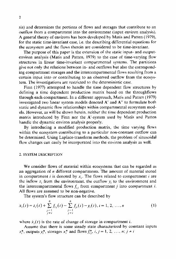
We consider flows of material within ecosystems that can be regarded as an aggregation of n different compartments. The amount of material stored in compartment i is denoted by xi. The flows related to compartment i are the inflow z~ from the environment, the outflow y, to the environment and the intercompartmental flows f,j from compartment j into compartment i. All flows are assumed to be non-negative.

The system's flow structure can be described by

±i(t)=z,(t)+ ~-~fij(t)- ~fj,(t)-y,(t),i=l,2 . . . . . n (1) j = l j = l j :~ i j=x i

where 5ci(t ) is the rate of change of storage in compartment i. Assume that there is some steady state characterized by constant inputs

z*, outputs y*, storages x* and flows f,~, i,j= 1, 2 . . . . . n;j:~i

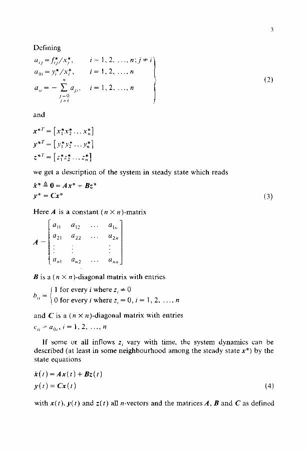
Def in ing

ai j =f i*2 /x* , i = 1, 2 . . . . . n ; j =~ i ]

ao, = y * / x * , i 1, 2 . . . . . n tl /

aii = -- E aji , i = 1, 2 . . . . . n [ j=O )

(2)

and

x * T = [ x ~ x ~ . . . X *]

y . T = [ y ~ y ~ . . . y . ]

we get a descr ip t ion of the system in s teady state which reads

.~* :~= 0 = A x * + BZ*

y * = Cx* (3)

H er e A is a cons tan t (n X n

a l l a12 . . . a ln

a21 a22 • . . a2n A __

anl an2 • . . ann

-matr ix

B is a (n x n)-diagonal matr ix with entries

1 for every i where z i ~ 0

b , = 0 for every i where z~ = 0, i = 1, 2, . . . , n

and C is a (n x n) -d iagonal mat r ix with entries

% = a 0 i , i = 1 ,2 . . . . , n

If some or all inflows z i vary with time, the system dynamics can be descr ibed (at least in some n e i g h b o u r h o o d among the s teady state x*) by the state equa t ions

5c(t) = A x ( t ) + B z ( t )

y ( t ) = C x ( t ) (4)

with x ( t ) , y ( t ) and z ( t ) all n-vectors and the matr ices A, B and C as def ined

4

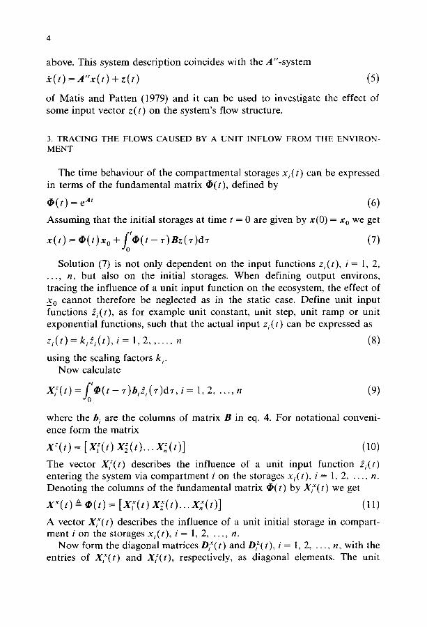
above. This system description coincides with the A"-system

=A"x(t) + z(t) (5)

of Matis and Patten (1979) and it can be used to investigate the effect of some input vector z( t) on the system's flow structure.

3. TRACING THE FLOWS CAUSED BY A UNIT INFLOW FROM THE ENVIRON- MENT

The time behaviour of the compartmental storages x , ( t ) can be expressed in terms of the fundamental matrix ~ ( t ) , defined by

• ( t ) = e TM (6)

Assuming that the initial storages at time t = 0 are given by x(0) = x 0 we get

x ( t ) = ~ ( t ) x o + fo t~ ( t - ' c )Bz ( ' c )d ' r (7)

Solution (7) is not only dependent on the input functions z~(t), i = 1, 2, . . . , n, but also on the initial storages. When defining output environs, tracing the influence of a unit input function on the ecosystem, the effect of x 0 cannot therefore be neglected as in the static case. Define unit input functions 2+(t), as for example unit constant, unit step, unit ramp or unit exponential functions, such that the actual input z~(t) can be expressed as

z , ( t ) = k i 2 i ( t ) , i = 1,2 . . . . . . n (8)

using the scaling factors k~. Now calculate

X : ( t ) = f o t C h ( t - . c ) b i e , ( z ) d . : , i = 1,2 . . . . . n (9)

where the b~ are the columns of matrix B in eq. 4. For notational conveni- ence form the matrix

XZ(t) = [ X : ( t ) X ~ ( t ) . . . X ~ ( t ) ] (10)

The vector X:( t ) describes the influence of a unit input function 2+(t) entering the system via compartment i on the storages x,(t) , i = 1, 2 . . . . . n. Denoting the columns of the fundamental matrix ~ ( t ) by X,~(t) we get

XX(t ) & ~ ( t ) = [ X ( ( t ) X ~ ( t ) . . . X ~ ( t ) ] ( l l )

A vector X~(t) describes the influence of a unit initial storage in compartment i on the storages xi( t ), i = l, 2 . . . . . n.

Now form the diagonal matrices DX( t) and D:( t), i = 1, 2 . . . . . n, with the entries of XX(t) and X:(t ) , respectively, as diagonal elements. The unit

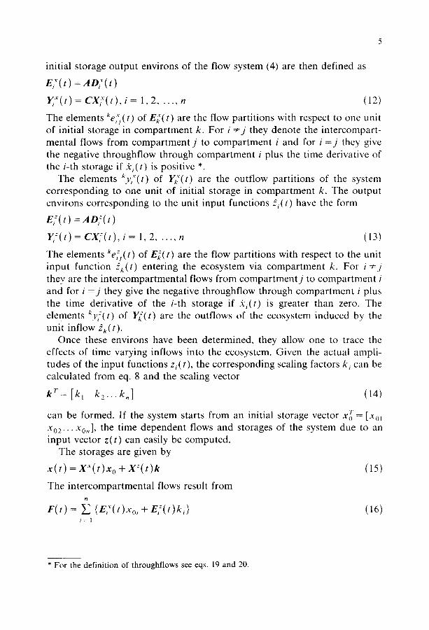
initial storage output environs of the flow system (4) are then defined as

E;"(t)=AO;~(t)

Y/'(t) = CX;~(t), i= 1,2 . . . . . n (12)

The elements x eij(t ) of Ei,~(t) are the flow partitions with respect to one unit of initial storage in compartment k. For i ~ j they denote the intercompartmental flows from compartment j to compar tment i and for i = j they give the negative throughflow through compartment i plus the time derivative of the i-th storage if 5c~(t) is positive *

The elements ky,~(t) of Yi,~(t) are the outflow partitions of the system corresponding to one unit of initial storage in compartment k. The output environs corresponding to the unit input functions di(t ) have the form

e . ( t ) = A o . ( t )

Y/( t ) = CX[(t), i = 1,2 . . . . . n (13)

The elements %,s(t) of E[,(t) are the flow partitions with respect to the unit input function £k(t) entering the ecosystem via compartment k. For i :x j they are the intercompartmental flows from compar tmen t j to compar tment i and for i = j they give the negative throughflow through compar tment i plus the time derivative of the i-th storage if 5c~(t) is greater than zero. The elements ky,:(t) of Y~(t) are the outflows of the ecosystem induced by the unit inflow dk(t ).

Once these environs have been determined, they allow one to trace the effects of time varying inflows into the ecosystem. Given the actual amplitudes of the input functions z~(t), the corresponding scaling factors k, can be calculated from eq. 8 and the scaling vector

k T= [k, k2 . . . k , ] (14)

can be formed. If the system starts from an initial storage vector x0 T = [xol x02.., x0,,], the time dependent flows and storages of the system due to an input vector z(t) can easily be computed.

The storages are given by

x ( t ) = x ' ( t ) x 0 + xz(t)k (15) The intercompartmental flows result from

n

F(t) = E (ET(t)Xoi + E;( t )k i ) (16) i = l

* For the definition of throughflows see eqs. 19 and 20.

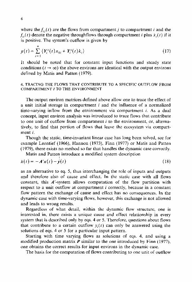
where t h e fij(t) are the flows from compartmentj to compartment i and the f . ( t ) denote the negative throughflows through compartment i plus 2i(t) if it is positive. The system's outflow is given by

y ( t ) = ~ (YiX(t)Xoi + YiZ(t)k,) (17) i=1

It should be noted that for constant input functions and steady state conditions (t ---) ~ ) the above environs are identical with the output environs defined by Matis and Patten (1979).

4. TRACING THE FLOWS THAT CONTRIBUTE TO A SPECIFIC OUTFLOW FROM COMPARTMENT 1 TO THE ENVIRONMENT

The output environ matrices defined above allow one to trace the effect of a unit initial storage in compartment i and the influence of a normalized time-varying inflow from the environment via compartment i. As a dual concept, input environ analysis was introduced to trace flows that contribute to one unit of outflow from compartment i to the environment, or, alterna- tively, to find that portion of flows that leave the ecosystem via compartment i.

Though the static, time-invariant linear case has long been solved, see for example Leontief (1966), Hannon (1973), Finn (1977) or Matis and Patten (1979), there exists no method so far that handles the dynamic case correctly.

Matis and Patten introduce a modified system description

.i:(t) = - A ' x ( t ) - ; ( t ) (18)

as an alternative to eq. 5, thus interchanging the role of inputs and outputs and therefore also of cause and effect. In the static case with all flows constant, this A'-system allows computation of the flow partition with respect to a unit outflow at compartment i correctly, because in a constant flow pattern the exchange of cause and effect has no consequences. In the dynamic case with time-varying flows, however, this exchange is not allowed and leads to wrong results.

Regardless of what detail, within the dynamic flow structure, one is interested in, there exists a unique cause and effect relationship in every system that is described only by eqs. 4 or 5. Therefore, questions about flows that contribute to a certain outflow yi(t) can only be answered using the solutions of eqs. 4 or 5 for a particular input pattern.

Starting with time varying flows as solutions of eqs. 4, and using a modified production matrix P similar to the one introduced by Finn (1977), one obtains the correct results for input environs in the dynamic case.

The basis for the computation of flows contributing to one unit of outflow

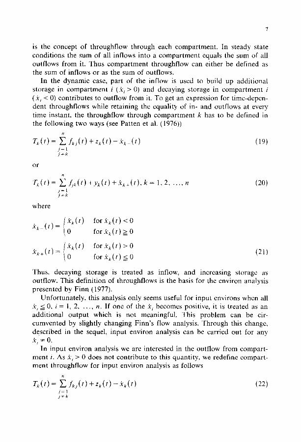
is the concept of throughflow through each compartment. In steady state conditions the sum of all inflows into a compar tment equals the sum of all outflows from it. Thus compar tment throughflow can either be defined as the sum of inflows or as the sum of outflows.

In the dynamic case, part of the inflow is used to build up additional storage in compar tment i (5c~ > 0) and decaying storage in compar tment i (5c~ < 0) contributes to outflow from it. To get an expression for time-dependent throughflows while retaining the equality of in- and outflows at every time instant, the throughflow through compar tment k has to be defined in the following two ways (see Patten et al. (1976))

Tk(t) = ~ f k j ( t )+zk( t ) - -SCk_( t ) (19) j = l j ~ k

o r

/7

Tk( t )= ~_, f jk ( t )+Yk( t )+SCk+(t ) ,k= 1,2 . . . . . n (20) ) = l j ~ k

where

5¢k+(t)= ( ~ k(t)

for 5Ck(t ) < 0

for 5¢k(t ) > 0

for 5Ck(t ) > 0

for 5Ck(t ) < 0 (21)

Thus, decaying storage is treated as inflow, and increasing storage as outflow. This definition of throughflows is the basis for the environ analysis presented by Finn (1977).

Unfortunately, this analysis only seems useful for input environs when all 5c i < 0, i = 1, 2 . . . . . n. If one of the 5c, becomes positive, it is treated as an additional output which is not meaningful. This problem can be cir- cumvented by slightly changing Finn's flow analysis. Through this change, described in the sequel, input environ analysis can be carried out for any 5c, ~ 0.

In input environ analysis we are interested in the outflow from compartment i. As 5¢~ > 0 does not contribute to this quantity, we redefine compartment throughflow for input environ analysis as follows

/q

Tk(t ) = Y'~ fk j ( t ) +Zk(t ) --SCk(t ) (22) j=l j=x k

or

n

Tk(t) = ~ f j k ( t ) + y k ( t ) , k = 1,2 . . . . . n (23) j = l j ~ k

These throughflows differ from eqs. 19 and 20 for ±k > 0 but they give exactly the amount of throughflow contributing to compartment outflow, regardless of the sign of 5ck(t ). Moreover, they coincide with the result for compartment throughflow in output environ analysis as given by the elements eii( t ) of environs E( t).

Based on this modified definition of throughflows, the production matrix P used by Finn has to be modified too for dynamic input environ analysis. This modified production matrix P for input environ analysis is of the order (4n x 4n) and has the form

- X n

T 1 P ( t ) = •

z 1

zl

zn

r1(£)

0 r~

Yl

• " Zn - X l " " " - X n r l . . . . . . Tn Y l " " " Yn

"z n ( t )

- ; ( ~ ( t ) 0

-Xn( t

0

0

0 . , f 1 2 ( t ) ' ' " f l n

f21 ( t ) ••

( t > . . . . . • o

( ~ )

] y 1 ( t ) I " " . . 0 J • • •

I 0 " . Y n ( t )

0

Starting with this production matrix, Finn's formulas for input environs apply without further change• The resulting throughflow partitions are identical with the originally defined throughflows from eqs. 19 and 20 for 5ci(t ) < 0 and differ from them by the amount of ±i+(t), which can easily be taken into account•

If we express the intercompartmental flows fu( t ) as fractions of the throughflows (22), namely

f u ( t ) = qij( t )T~( t ) (25)

(24)

eq. 23 can be rewritten as

L ( t ) = ~ qjk( t )Tj ( t )+yk( t ) (26) / = 1

Denoting the (n × n)-matrix with entries qij(t) Q22(t), the instanteneous throughflows that contribute to the output vector y(t) can be written as

TT(t) = yr ( t ) [ I -- Qzz(t)]--1 (28)

Writing the production matrix P(t) as

0 0 0 2n

e( t )= e~,(t) e2~(t) o . 0 P32 ( / ) 0 n

and dividing every non-zero element in each row of P(t) by the corresponding row sum yields the matrix

0 0 0

Q ( t ) = Q: , ( t ) Q22(t) 0 (29)

0 Q32(/) 0

Now define the (4n × 4n)-matrix

[, o N ( t ) = [ l - Q ( t ) ] - l = N21(t) N22(t)

N~,(t) N~:(t)

where the following relationships hold (see Finn, 1977)

N22(t) = [ I - 0 2 2 ( t ) ] - '

Jv2,(t) = N2~(t)Q2,(t)

N3,(t) = Q3~(t)N~,(t)

N32(t ) = Q3z(t)Nz2(t)

(30)

(31)

Then the partition of inflows, time derivatives of storages and compartmental throughflows in terms of the input vector y(t) is given by

[ z r ( t ) - k r ( t ) i T f ( t ) i y r ( t ) ]=yr ( t ) [N3 , ( t ) ! N32(t) ! I] (32)

The rows nr,(t), i = 1, 2 . . . . . n of the matrix

[N3,(t ) N32(t ) I ] {33)

10

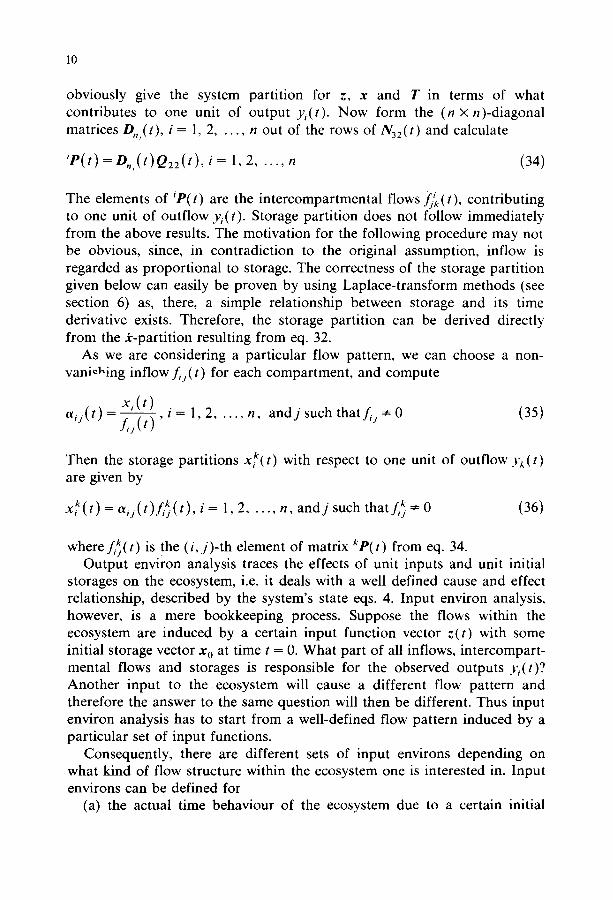
obviously give the system partition for z, x and T in terms of what contributes to one unit of output y~(t). Now form the (n × n)-diagonal matrices D,,( t ) , i = 1, 2 . . . . . n out of the rows of N32(t ) and calculate

' P ( t ) = D . , ( t ) Q 2 2 ( t ) , i = 1, 2 . . . . . n (34)

The elements of ip( t) are the intercompartmental flows fj~.(t), contributing to one unit of outflow y,( t) . Storage partition does not follow immediately from the above results. The motivation for the following procedure may not be obvious, since, in contradiction to the original assumption, inflow is regarded as proportional to storage. The correctness of the storage partition given below can easily be proven by using Laplace-transform methods (see section 6) as, there, a simple relationship between storage and its time derivative exists. Therefore, the storage partition can be derived directly from the k-partition resulting from eq. 32.

As we are considering a particular flow pattern, we can choose a non- vanishing inflow f , j ( t ) for each compartment, and compute

a i j ( t ) - x i ( t ) f / i ( t ) ' i = 1,2 . . . . . n, a n d j such that f,j * 0 (35)

Then the storage partitions x~( t ) with respect to one unit of outflow yk(t) are given by

x ~ ( t ) = a , j ( t ) f , ~ ( t ) , i = 1,2 . . . . . n, a n d j such that f,~ :~0 (36)

wheref ,~( t ) is the ( i , j ) - t h element of matrix kP( t ) from eq. 34. Output environ analysis traces the effects of unit inputs and unit initial

storages on the ecosystem, i.e. it deals with a well defined cause and effect relationship, described by the system's state eqs. 4. Input environ analysis, however, is a mere bookkeeping process. Suppose the flows within the ecosystem are induced by a certain input function vector z(t) with some initial storage vector x 0 at time t = 0. What part of all inflows, intercompartmental flows and storages is responsible for the observed outputs .v,(t)? Another input to the ecosys tem will cause a different flow pattern and therefore the answer to the same question will then be different. Thus input environ analysis has to start from a well-defined flow pattern induced by a particular set of input functions.

Consequently, there are different sets of input environs depending on what kind of flow structure within the ecosystem one is interested in. Input environs can be defined for

(a) the actual time behaviour of the ecosystem due to a certain initial

11

storage vector x 0 and to a given input vector z ( t ) . This results in a set of n input environs, where it is understood that input environs corresponding to y, ( t ) - 0 simply vanish,

(b) the flows induced by a given initial storage vector x o and the actual input vector z ( t ) separately. This results in a set of 2n input environs, or

(c) every output environ. This results in a set of 2n 2 possible input environs for an n-th order system.

As the time behaviour of an ecosystem due to arbitrary input functions z,( t) can be quite complex, dynamic input environ analysis may become a tedious task unless numerical techniques are used. When investigating the effect of all causes separately--i .e, case ( c ) - - the structure of every single input environ will be less complicated, but there will be 2n 2 of them!

In dynamic flow analysis the outflows y~(t) are t ime-dependent too, and therefore the amount of flow contributing to "one unit of outflow from compar tment i " is given by fractions with time functions in the denomina- tor. It seems more meaningful to ask for the portion of flows contributing to the actual outflow y , ( t ) from compar tment i. This type of input environ can be obtained from the above results by multiplying every input environ by the corresponding time function y, (t).

In applications of dynamic flow analysis two kind of time functions will be encountered most frequently: stepwise and sinusoidal input functions. In the sequel, these two types of time-varying inflows will be considered in more detail.

5. STEPWISE INPUT FUNCTIONS

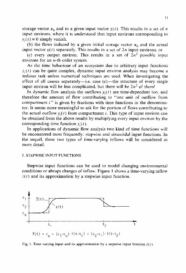
Stepwise input functions can be used to model changing environmental conditions or abrupt changes of inflow. Figure 1 shows a time-varying inflow z(t) and its approximation by a stepwise input function.

c I

c 2

C 0

z ( t )

t I t 2 t

~ ( t ) = c o + ( C l - C o ) ' l ( t - t l ) + ( c 2 - c l ) ' l ( t - t 2 )

Fig. 1. Time varying input and its approximation by a stepwise input function ,~(t).

12

Example 1. in Fig. 2.

The state equations for this system are given by

,(t)=Ax(t)+nz(t) y( t )=Cx( t ) with

A = 4 / 3 - 7 / 3 ] ' B = 1 '

Consider the following flow model, whose steady state is shown

(37)

j31 Assume that, starting from these steady state flows and storages, the inputs z 1 and z 2 change from z r = [3 3] to z r = [1/3 10/3] at some time instant to, which can arbitrarily be set to t o = 0 as we are dealing with time-invariant systems.

The input functions therefore are given by

Zl(t) = 1 / 3 . l ( t ) and

Zz(t ) = 1 0 / 3 . l ( t )

with the initial storage vector Xo r = [3 3] Denot ing the unit input functions by 2~(t) = 22(t) = l( t ) we have

1,7-= [1/3 10/3] First consider the output environs for this system.

With

XX(t) = ~ ( t ) = / 2 / 3 e - t + 1/3 e-3t

2 / 3 e - ' - 2 / 3 e-3 '

matrix (10) becomes

x=(t)= [

1/3 e - ' - 1 /3 e "3']

1 /3 e - ' + 2 / 3 e -3' 1

-~- } e - ' - } e-3' 9 2 ½e-, + }e-3,]

- 3 2 e - ' + 2 e - 3 ` 95 ½ e - ' - } e -3'

4

zi=3 ~ I x I = 3 x 2 = 3 -I

qr it"

Yl =1 Y2=5

Fig. 2. Flow model in steady state.

-k

I ~ z2=3

I -

13

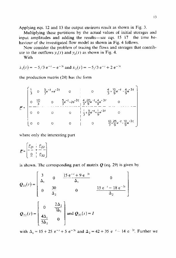
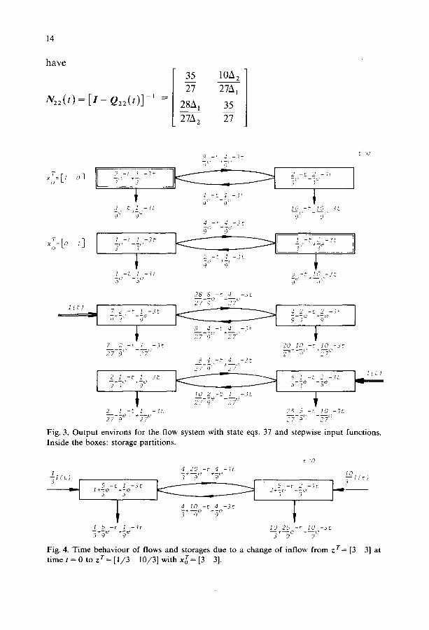
Applying eqs. 12 and 13 the output environs result as shown in Fig. 3. Multiplying these partitions by the actual values of initial storages and

input amplitudes and adding the resul ts - -see eqs. 1 5 - 1 7 - - t h e time behaviour of the investigated flow model as shown in Fig. 4 follows.

Now consider the problem of tracing the flows and storages that contribute to the outflows yl( t ) and y2(t ) as shown in Fig. 4.

With

2 , ( t ) : - 5 / 3 e - ' - e - 3 ' a n d 2 2 ( t ) = - 5 / 3 e - ' + 2 e 3,

the production matrix (24) has the form

p' =

I 5 - t -3t 0 5e +e 0

0 10 5 - t ~ - 3 t "~- 0 5 e - z e

0 0 0 0

0 0 0 0

0

4 20-t 4 -3t 5+ge +ge

1 5 - t + l e - 3 t 5+g e

0

4 10 -t 4 - 3 t 5 + ge - g e

O

10 25 - t I0 -3t -g+g~ - g e J

where only the interesting part

e'=--7, e, j is shown. The corresponding part of matrix Q (eq. 29) is given by

Q2, ( / ) =

3 15 e - ' + 9 e - 3 '

A~- 0 Ai 0

30 15 e - ' - 18 e - 3 t 0 0

A 2 A 2

Q22(t) =

2A 2 0

7A 1

4Al 0

5A 2

and Q 3 2 ( t ) = ]

with AI = 15 + 25 e - ' + 5 e -3t and A 2 = 42 + 35 e -~ - 14 e - 3 t . Further we

14

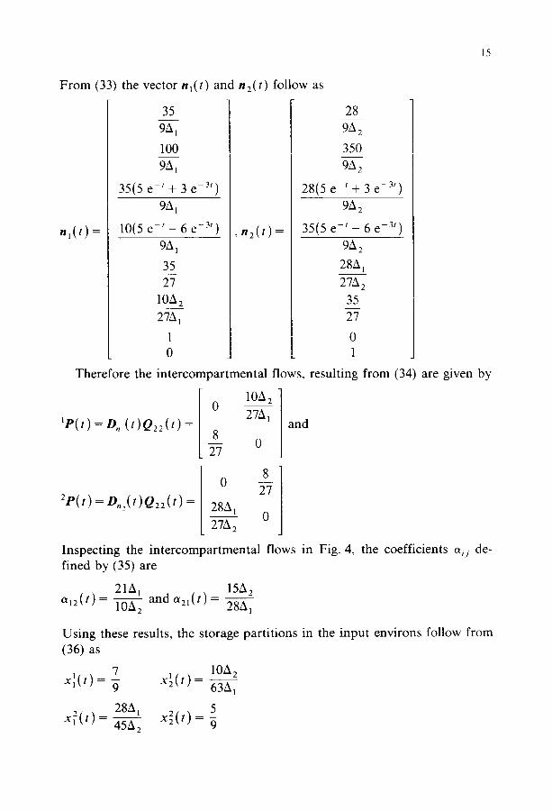
h a v e

N22( t )= [ l - Q22( t ) ] - ' =

35 10A 2

27 27A l

28A 1 35

27A 2 27

xT=[I 03 o

Tr 1] xo= LO

1( c) _..]

-I

$ -t $ -?t o

-o 70 2 ) -jc

2 -t l -~t lO -t IO -3t ?e +;c' ~c' -~e, 4 -t 4 -3t

I -t 1 -3t I -t 2 -3t 5 ~ +]÷

2 -c 4 -3t

1 -t i -3t 5 -t i0 -3t

t 0

28 8 -t 4 -3t

7 2 -t 1 -3t I [ 4 2 -c 2 -3t ~--c -7)e ~ ~ 72-~c +~e

8 4-t 4 -3t ~-7-~ 0 +2--~e

7 2-t 1 -3t 20 i0 -t 10 -3c - • 27 • +~e

$ 4 -t 4 -3t 277- ~2 e + - - 7

2 i -t I -3t ~ 5 : -t 2 -3t L.~ 1{cj

9 3 ~ 9 9 3

~ - ~)~ ---~2 z 2 I - t 1 - 3 t 25 5 - t I 0 - 3 C

Fig. 3. Output environs for the flow system with state eqs. 37 and stepwise input functions. Inside the boxes: storage partitions.

i 4 20 -t+4e-3t l ( t ) -~+--~e

- - q 1+5e-t+le-]t ~

I 4 i0 -t 4 -3t 3 9

1 5 -t 1 -3t

['0

I O I ( t )

5 t 2 -3~ - - [ 3 2+~e -]~ r"

IO 25 -t 10 -3t

Fig. 4. Time behaviour of flows and storages due to a change of inflow from z r= [3 t i m e t = 0 t o z r = [ 1 / 3 10/3] wi thx r= [3 3].

3] at

15

From (33

h i ( t ) =

the vector n I (t) and n 2 ( t) follow as

35 9A~

100 9Aj

35(5 e - ' + 3 e -3t)

9A1

10(5 e - ' - 6 e -3t)

9A 1

35 27

10A2

27A~

1 0

28

9A 2

350

9A 2

28(5 e ' + 3 e -3')

9A 2

35(5 e - t - 6 e -3')

9A 2

28A 1

27A 2

35 27

0 1

Therefore the intercomgartmental flows, resulting from (34) are given by

I0A 2 0

~P(t) =Dn,(t)Q22(t) = 8 27A1 and

0 27

2 e ( t ) = O o , ( t ) Q 2 2 ( t ) =

8 0

27

28A1 0 27A 2

Inspecting the intercompartmental fined by (35) are

21A1 and a21(t ) _ 15A2 O~12 ( / ) = 10A----~ 28A 1

flows in Fig. 4, the coefficients a,~. de-

Using these results, the storage partitions in the input environs follow from (36) as

7 x~(t)- lOA2

2 2 ( / . ) . 2 8 A 1 x2(t ) 5 45A2 = -~

16

35 8 27 i00

--5 Z ~ ~o~ 1_ 9~,,

1 27'^~

28A~

28 27'!~2 350

27 1

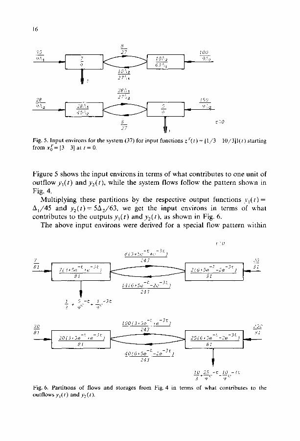
Fig. 5. Input environs for the system (37) for input functions zr(t) = [1/3 fromx0 r = [ 3 3] at t = 0 .

t>O

lO/3] l ( t ) starting

Figure 5 shows the input environs in terms of what contributes to one unit of outflow y~(t) and y2(t), while the system flows follow the pattern shown in Fig. 4.

Multiplying these partitions by the respective output functions .vl(t) = A J 4 5 and y2(t)= 5A2/63, we get the input environs in terms of what contributes to the outputs yl(t) and y2(t), as shown in Fig. 6.

The above input environs were derived for a special flow pattern within

~kO

-3t 8(3+5e-t+e ) 7 243 20

7(3+5e-t+e-3t) -t -3t 2(6+5e -2e ) 87 8I

I 14(6+5e_t_2e_3t) 243

I 5 -t I -3t 7 + ~e + ~e

2O lO0(3+5e-t+e-3t) 25C

243 2 0 ( 3 * 5 0 +e ) 2 5 ( 6 + 5 e - t - 2 e - 3 t )

40(6+5e-t-2e-3t243 I

I0 25 -t 10 -3t -- 9 --~ e

m terms of what contributes to the Fig. 6. Partitions of flows and storages from Fig. 4 outflows yl(t) and yE(t).

17

the system, i.e. case (a). Four different partitions would have resulted by considering the influence of the initial vector x0 r = [3 3] and of the input vector z r = [1/3 10/3]. l( t) separately (case (b)) and eight would have resulted from investigating input environs for every output environ (case (c)). It is obvious that every set of input environs will have a different structure, reflecting the fact that an input environ cannot be defined (except in the static case), regardless of the actual flows within the system. Calculating input environs for every output environ is a tedious task, but the results would be independent of the actual flow behaviour in the sense that they could be used to congregate input environs for arbitrary initial vectors x 0 and arbitrary scaling vectors k.

The vectors n~ contain additional information on the throughflows, not shown in Figs. 3-6. The T,k(t) are the throughflows through compartment i, contributing to the outflow yk(t) as defined by eqs. 22 and 23. The results for the 5c~(t) can be used to calculate the throughflows as defined by eqs. 19 and 20 according to the usual definition of throughflows.

6. T R A N S F E R F U N C T I O N S A N D E N V I R O N A N A L Y S I S

In systems theory, different methods exist for the analysis of linear, time-invariant systems. Besides the time-domain state space methods, Laplace transformation is a useful tool to investigate the dynamic behaviour of these systems. Using Laplace-transform methods, linear differential equations are transformed into linear algebraic equations, thus simplifying the solution techniques. Moreover, this method is especially well suited for investigating the influence of harmonic input functions. Within ecosystems, harmonic input functions can occur through fluctuations like annual or daily cycles, etc. These input functions can vary around an average value and shall be considered sinusoidal in the sequel.

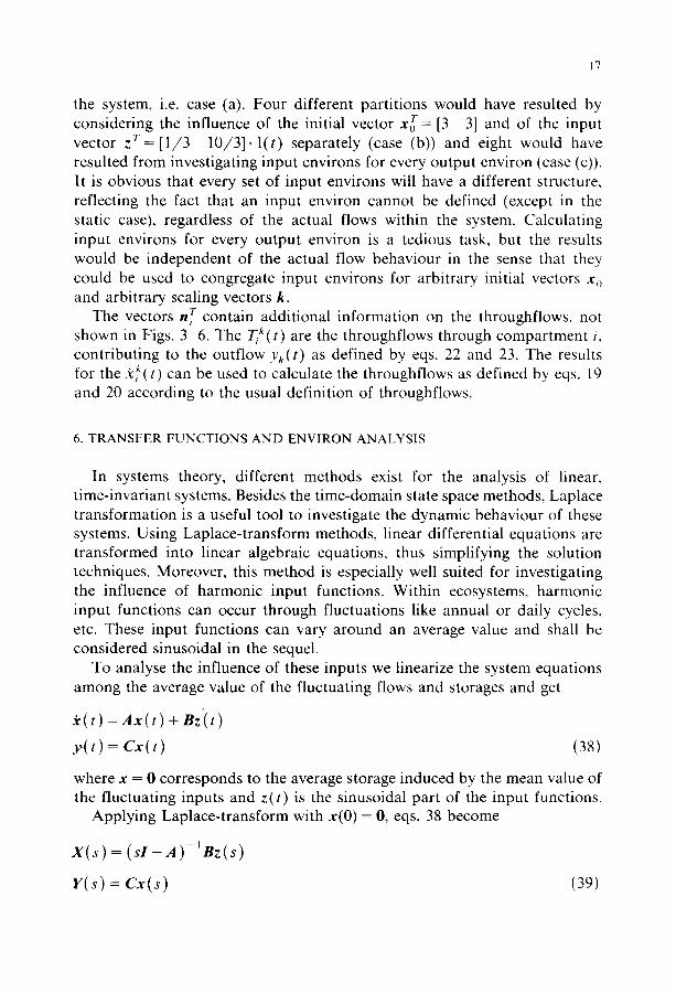
To analyse the influence of these inputs we linearize the system equations among the average value of the fluctuating flows and storages and get

• (t) = A x ( t ) +

y ( t ) = Cx( t ) (3S)

where x = 0 corresponds to the average storage induced by the mean value of the fluctuating inputs and z( t) is the sinusoidal part of the input functions.

Applying Laplace-transform with x(0) = 0, eqs. 38 become

X(s) = ( s X - A ) - ' n z ( s )

r(s)=Cx(s) (39)

18

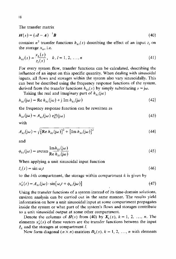
The transfer matrix

H ( s ) = ( s l - A ) - l B (40)

contains n 2 transfer functions hkt(s ) describing the effect of an input z t on the storage x k, i.e.

h,,(s)_ x*(s) z , ( s ) ' k , l = 1 , 2 . . . . ,n (41)

For every system flow, transfer functions can be calculated, describing the influence of an input on this specific quantity. When dealing with sinusoidal inputs, all flows and storages within the system also vary sinusoidally. This can best be described using the frequency response functions of the system, derived from the transfer functions hk~(s ) by simply substituting s =j~0.

Taking the real and imaginary part of hkl(jO~ ) hk,(jo~) = Re hk,( j~) + j am hk,(jb~ ) (42)

the frequency response function can be rewritten as

hk,(j~0) = Akz(j~0 ) eft (j~0) (43)

with

A k , ( j ~ ) = v/[Re h~,(. jw)] 2 + [Im h,,(jo~)] 2 (44)

and

Imhkl(jo~ ) q~k,(j0~) = arctan (45)

Re h kl (j~ )

When applying a unit sinusoidal input function

e , ( t ) = sin ~,t (46)

to the l-th compar tment , the storage within compar tment k is given by

x ~ ( t ) = Ak,(j~o). sin[ ~,t + q~k, (j~0)] (47) i

Using the transfer functions of a system instead of its t ime-domain solutions, environ analysis can be carried out in the same manner. The results yield informat ion on how a unit sinusoidal input at some compar tment propagates inside the system or what part of the system's flows and storages contr ibute to a unit sinusoidal output at some other compar tment .

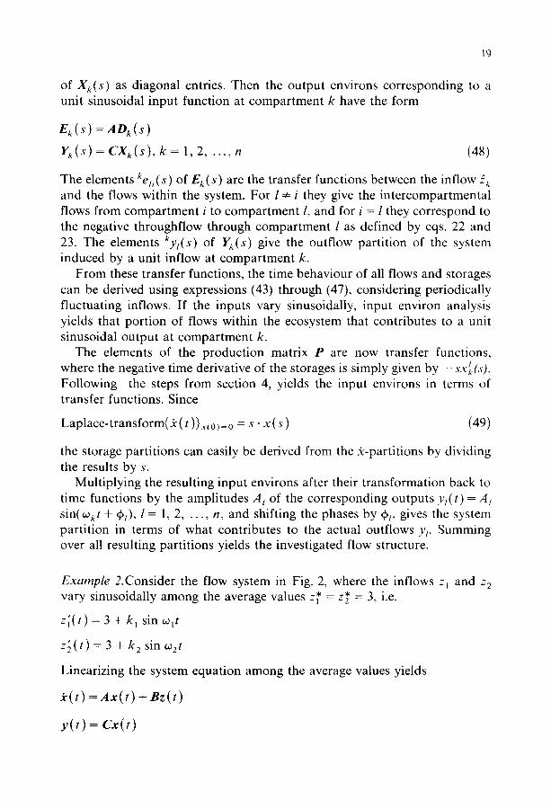
Denote the columns of H ( s ) f rom (40) by X k ( s ), k = 1, 2 . . . . . n. The elements x~(s ) of these vectors are the transfer functions between the input 2 k and the storages at compar tment l.

Now form diagonal (n × n)-matrices Dk(s ), k = 1, 2 . . . . . n with elements

19

of Xk(s ) as diagonal entries. Then the ou tput environs corresponding to a unit sinusoidal input function at compar tmen t k have the form

Ek(s) =AOk(s) Yk(s) = CX~(s) , k = 1, 2 . . . . . n (48)

The elements % , ( s ) of Ek(s ) are the transfer functions between the inflow 2 k and the flows within the system. For l * i they give the in tercompar tmenta l flows from compar tment i to compar tment l, and for i = l they correspond to the negative throughflow through compar tmen t l as defined by eqs. 22 and 23. The elements kyt(s ) of Yk(s) give the outflow part i t ion of the system induced by a unit inflow at compar tment k.

F rom these transfer functions, the time behaviour of all flows and storages can be derived using expressions (43) through (47), considering periodically fluctuating inflows. If the inputs vary sinusoidally, input environ analysis yields that port ion of flows within the ecosystem that contributes to a unit sinusoidal output at compar tment k.

The elements of the product ion matrix P are now transfer functions, where the negative time derivative of the storages is simply given by -sx~(s) . Following the steps f rom section 4, yields the input environs in terms of transfer functions. Since

Laplace-transform(So ( t )) x~0)= 0 = s . x ( s ) (49)

the storage parti t ions can easily be derived from the 5c-partitions by dividing the results by s.

Multiplying the resulting input environs after their t ransformation back to t ime functions by the ampli tudes A~ of the corresponding outputs Yt(t) = A~ sin(~0kt + +~), l = 1, 2 . . . . . n, and shifting the phases by q,~, gives the system part i t ion in terms of what contributes to the actual outflows Yr. Summing over all resulting parti t ions yields the investigated flow structure.

Example 2.Consider the flow system in Fig. 2, where the inflows z 1 and z 2 vary sinusoidally among the average values z~ = z~' = 3, i.e.

z~(t) = 3 + k 1 sin wtt

z'z(t ) = 3 + k 2 sin w2t

Linearizing the system equat ion among the average values yields

J c ( t ) = A x ( t ) + B z ( t )

ytt)=Cx(t)

20

with

A = 4 /3 - 7 / 3 ' B = 0 1

and

C = [ O

The output environs follow from (48) as

I - 5 ( 3 s + 7 ) 8 3A 3A yl ( s ) =

E l ( s ) = 4(3s+ 7) --28 '

3A 3A

and

E2(s ) =

Xl(S)=

3 s + 7 A 4 A

andX2(s ) =

2 A

3 s + 5 A

- 1 0 2 (3s+5) ] 3A 3A

l 8 - 7 ( 3 s + 5 ) ' Vz(s)= 3A 3A

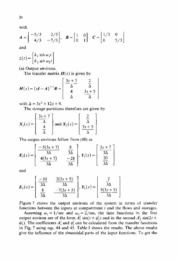
Figure 7 shows the output environs of the system in terms of transfer functions between the inputs at compartment i and the flows and storages.

Assuming wl = 1/see and o~ z = 2/see, the time functions in the first output environ are of the form All sin(t + ~l) and in the second At2 sin(2t + 4)~). The coefficients A I and 4)1, can be calculated from the transfer functions in Fig. 7 using eqs. 44 and 45. Table I shows the results. The above results give the influence of the sinusoidal parts of the input functions. To get the

3 s + 7 3A 20 3A

2 3A

5(3s + 5) 3A

[k~ sin O~lt ] z ( t ) = k2 sin o~2t ]

(a) Output environs. The transfer matrix H ( s ) is given by

3 s + 7 2

m s ) = ( s I - A ) - ' n = A a 4 3 s + 5 A A

with A = 3 s 2 + 12s + 9. The storage partitions therefore are given by

21

(a)

(b)

1 __1 " 3 s + 7 :] 5

i 3s+7

7 ,'X

2

1 2

3£

4(7s+7)

T

? ?,

2O ?/?,

8

3S÷5

2 ( 7 S + 5 ) 1 !

5 ( C ~ + 5 )

7,',

Fig. 7. Output environs in terms of transfer functions.

complete picture, the steady state corresponding to the average values has to be added. (b) Input environs.

Induced by the sinusoidal parts of the inflow, the outflows vary sinusoidally too at the same frequency. As z] and z 2 have different frequencies, it is favourable to investigate the propagation of zj and z z separately.

Thus we get two sets of input environs corresponding to the two output environs in Fig. 7. Taking the flows from Fig. 7a, the production matrix reads

P I ( s ) =

1 0 - ( 3 s 2 + 7 s ) 0 I 8 "

- 4 s I 4 ( 3 s + 7 ) 0 0 0 O

A I 3A I 3 s + 7

0 0 0 0 I 3A 0 I 2O

o o o O l 0 3--Z

where again only the interesting parts of P and Q are considered. The production matrix for the flows with frequency (D2 reads

P 2 ( s ) = I O 0

0 I

0 0

0 0

-2_{s 0 I 0 2 (3s+5 ) A I 3A

0 - ( 3 s Z ÷ S s ) 1 8 0 A I 3 A

I "J o o ~'-- o

13A 5 ( 3 s + 5 )

0 0 I 0 3A

22

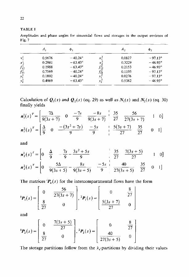
T A B L E I

A m p l i t u d e s and phase angles for s inusoidal f lows and s torages in the o u t p u t envi rons of

Fig. 7

AI q~1 A2 q~2

x I 0.5676 - 40.24 ° x2 0.0827 - 97.13°

x~ 0.2981 - 63.43 ° x 2 0.3229 - 46.93 °

f]2 0.1988 -- 63"43° f?2 0.2153 - 46.93 °

f ~ 0.7569 - 4 0 . 2 4 ° fzz~ 0.1103 - 97.13 °

y~ 0.1892 _ 40.24 ° y2 0.0276 - 97.13 °

y2 ~ 0.4969 - 63.43 ° y2 z 0.5382 - 46.93 °

Calculation of Ql(s) and 0 2 ( S ) (eq. 29) as well as Nt(s ) and N2(s ) (eq. 30) finally yields

7 A - 7 s - 8s nl(s )r= 9(3s+7) 0 9 9 (3s+7)

[ A --(3s 2 + 7s) --5s n2(S) T = 9 0 [ 9 9

35 56 27 27(3s + 7)

5(3s + 7) 35 27 27

1 o]

0 1]

and

A 7s 3 s 2 + 5 s n~(s) r= 0 -~ -~ 9

5A 8s - 5s nZ(s) r= 0 9(3s+5) 9 (3s+5) 9

35 7(3s + 5) 27 27

40 35 - - 0

27(3s + 5) 27

o]

1]

The matrices iPk(s ) for the intercompartmental flows have the form

) 5(3s + 7) 8

56 0 27 0 27(3s + 7 ) , 2p,(s) =

' e , ( s ) = __8 o o 27 27

and

' e 2 ( s ) =

0 7(3s + 5) ]

27 J 2P2(s) = 8 0 '

27

8 0 27

40 0

27(3s + 5)

The storage partitions follow from the ±i-partitions by dividing their values

23

' x I ( s ) ' x2(s)-

and

by s (or via the formulas presented in section 4) as

8 3 s + 7 9(3s + 7) ' lxZ(s) - 9 ' 'x2(s)= ~

3 s + 5 8 2 1 2 1 2x2,s,, 2 x , ( s ) = { , x2(s ) - 9 ' 9 ( 3 s + 5 ) ' x 2 ( s ) = {

Figure 8 shows the two sets of input environs partitioning the system into portions that contribute to a unit output sine function at frequency o0 = o01 and o0 = o02.

For 21(t ) = sin t, the time functions in the environs of Fig. 8a have the form A/~ sin(t+~/1). Table II shows the corresponding amplitudes and phases. As 22(t ) = sin 2t, the time functions in the input environs from Fig. 8b have the form A~ sin(2t + ~ ) . Table III shows the amplitudes and phases of flows and storages in Fig. 8b.

8

7,',~ 2 7

~(>:+7) __I 7_ ~ s

~] 9 9(3s+7)

2 7 ( 3 5 ÷ 7 ) I

5(3s+7) 27

__1 3s+ 7 ~ 5_ --1 9 9

8 27

,5 0

(a)

8 - - k , 2 7

7 ~ 3~+5 L_ 9 9 9 I ~

7(3s+5) 27

1

(b)

,I 0 5£

27(3s+5)

9(3s+5) 9 ,] - -

27 1

Fig. 8. Input environs in terms of transfer functions. (a) Input environs for the flows at frequency ~ = %. (b) Input environs for the flows at frequency oa = w 2.

24

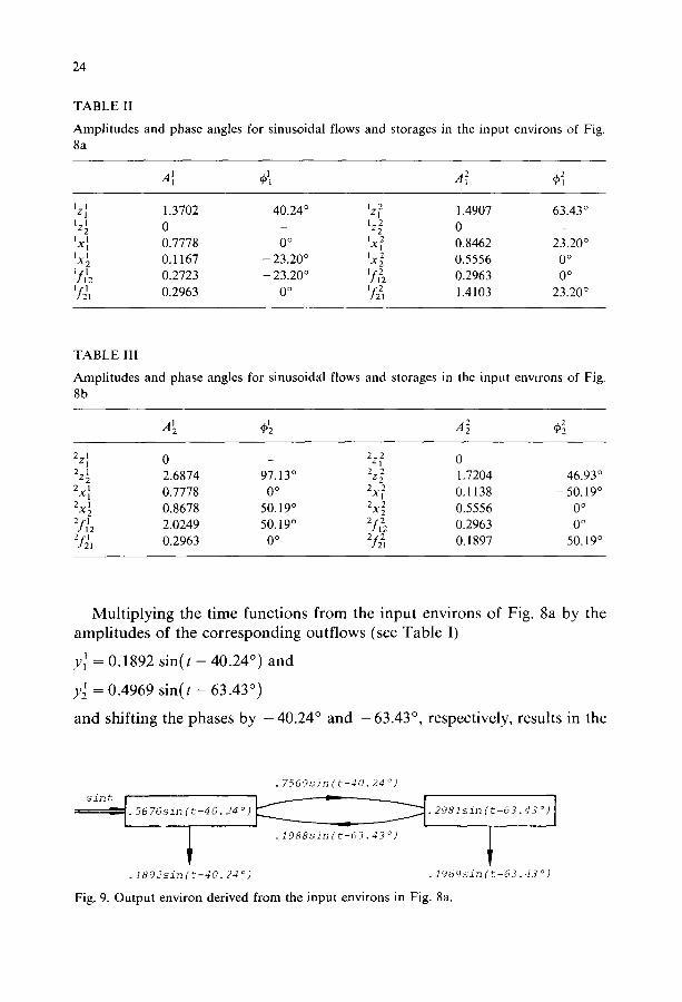
TABLE II

Amplitudes and phase angles for sinusoidal flows and storages in the input environs of Fig. 8a

.4,, 4,

~z ~ 1.3702 40.24 ° 1 z 2 1.4907 63.43 o IZ~ 0 -- 122 0 -

Ix l 1 0.7778 0 ° IX l 2 0.8462 23.20 ° lX~ 0.1167 -- 23.20 ° 1X22 0.5556 0 ° 1f~2 0.2723 -- 23"20° ~f~2 0.2963 0 ° ~f~l 0.2963 0 o lf2j 1.4103 23.20 °

TABLE III

Amplitudes and phase angles for sinusoidal flows and storages in the input environs of Fig. 8b

2 1 0 2Z? 0 Z 1 2z~ 2.6874 97.13 ° 2z 2 1.7204 46.93 ° 2X I 0.7778 0 ° 2X( 0.1138 -- 50.19 ° 2X~ 0.8678 50.19 ° 2X~ 0.5556 0 ° 2f~ 2 2.0249 50.19 ° 2f~ 0.2963 0 ° 2f~ 1 0 . 2 9 6 3 0 ° 2f~ I 0.1897 -- 50.19 °

M u l t i p l y i n g t h e t i m e f u n c t i o n s f r o m t h e i n p u t e n v i r o n s o f F ig . 8a b y t h e

a m p l i t u d e s o f t h e c o r r e s p o n d i n g o u t f l o w s ( see T a b l e I )

y~ = 0 . 1 8 9 2 s i n ( t - 4 0 . 2 4 °) a n d

y~ = 0 . 4 9 6 9 s i n ( t - 6 3 . 4 3 °)

a n d s h i f t i n g t h e p h a s e s b y - 4 0 . 2 4 ° a n d - 6 3 . 4 3 °, r e s p e c t i v e l y , r e s u l t s i n the

.56 76sin ( t-40. 24 o)

. 1 8 9 2 s i n ( t - 4 0 . 2 4 o)

.7569sin(t-40.24 °)

~.2981sin(t-63.430) I

• 1988sin(t-63"43°) I

• 4969sin (t-63.43 o)

Fig. 9. Output environ derived from the input environs in Fig. 8a.

25

flow partitions in terms of what contributes to the outflows y~(t) and y~(t) induced by a unit input flow dl(t) = sin t. Adding the results gives the output environ shown in Fig. 9, which corresponds to the one from Fig. 7a.

The above results show that transfer function methods are well suited for tracing the periodically fluctuating parts of flows in an ecosystem.

7. C O N C L U S I O N S

The purpose of this paper was to extend known, static, input -ou tput environ analysis for time-invariant linear intercompartmental systems to the case of time-varying input functions. For the first time, consistent results between input-environs and output-environs for the dynamic inflow case are developed. This development rectifies several previous attempts to solve this problem by other authors (Finn, 1977; Matis and Patten, 1979).

An ecologically interesting family of non-constant input functions are harmonic inflows. The environ analysis of such forcings can be elegantly facilitated via a simple reformulation of the environ analysis in terms of Laplace transformed quantities.

Though the assumptions of linearity may not be completely justified in a real system under global conditions, linear systems theory is a powerful tool to investigate most classes of systems so long as the system is operating near an equilibrium or working point and its dynamic inputs do not drive the system too far away from this working point.

Many ecosystems are better modelled by time-dependent differential equations, since virtually all physiological processes are temperature dependent and temperature itself follows a well defined temporal dynamic. Ecosystem models involving such processes are naturally time varying. Consequently the present investigation should also be extended to this case.

On the other hand, some ecosystems exhibit a distinctive complex behaviour which cannot be satisfactorily approximated by even complicated time dependent linear forms. Therefore, it would be desirable to develop a non-linear environ analysis for either general or specific classes of non-linear systems. Although such an analysis would not be isomorphic to the analysis presented herein, certainly there would exist analogous formulations of concepts between these two types of analysis.

A C K N O W L E D G M E N T S

The work was done while the author was with the Institute of Ecology, University of Georgia, Athens, Georgia, U.S.A. He is particularly indebted to Dr. B.C. Patten who brought the problem to his attention and he is very grateful to Craig M. Barber for his stimulating discussions and helpful remarks.

26

REFERENCES

Barber, M.C., 1978. A Markovian model for ecosystem flow analysis. Ecol. Modelling, 5: i 93-206.

Finn, J.T., 1977. Flow Analysis: A Method for Tracing Flows Through Ecosystem Models. Ph.D. Thesis, University of Georgia, Athens. GA.

Hannon, B., 1973. The structure of ecosystems. J. Theor. Biol., 41: 535-546. Leontief, W.W., 1966. Input-Output Economics. Oxford University Press, New York, pp.

134-155. Matis, J.H. and Patten, B.C., 1979. Environ Analysis of Linear Compartmental Systems: The

Static, Time Invariant Case. Proc. 42nd Session, Int. Stat. Inst., Manila, Philippines, December 4-14 (in press).

Patten, B.C., 1978. Systems approach to the concept of environment. Ohio Journal of Science. 78: 206-222.

Patten, B.C., Bosserman, R.W., Finn, J.T. and Cale, W.G., 1976. Propagation of cause in ecosystems. In: B.C. Patten (Editor), Systems Analysis and Simulation in Ecology. Vol. 4. Academic Press, New York, NY, pp. 457-579.

environ analysis of linear compartmental systems: the dynamic, time-invariant case

Documents