Entropy Coe¢ cient of Determination and ItsApplication

Nobuoki Eshima

Department of Biostatistics, Faculty of Medicine, Oita University, Oita

879-5593, Japan.

E-mail: eshima@oita-u.ac.jp

The objective of this seminar is to introduce the entropy co-

e¢ cient of determination (ECD) for measuring the explanatory

or predictive power of GLMs and to consider how ECD is used

in data analysis. In the �rst section, the classical regression and

GLM frameworks are compared, and properties of GLMs concern-

ing entropy are discussed. First, the information of an event and

the entropy of a random variable are explained, and the Kullback-

Leibler information that describes the di¤erence between two dis-

tributions is treated. Second, the log odds ratio and the mean

in the GLM are considered from a view point of entropy. ECD

is interpreted as the ratio of variation of a response variable ex-

plained by the explanatory variables, and is compared with some

other explanatory power measures with respect to the following

properties: (i) interpretability; (ii) being the multiple correlation

coe¢ cient or the coe¢ cient of determination in normal linear re-

gression models; (iii) entropy-based property; (iv) applicability

1

to all GLMs; in addition to these, it may be appropriate for a

measure to have the following property: (v) monotonicity in the

complexity of the linear predictor. In Section 2, �rst the asymp-

totic properties of the maximum likelihood estimator (MLE) of

ECD are discussed. The con�dence interval of ECD is consid-

ered on the basis of an approximate normality of non-central chi

square distribution. Second, in canonical link GLMs the contri-

butions of factors are treated according to the decomposition of

ECD. Numerical examples are also given.

1 Coe¢ cient of determination for generalized

linear models

1.1 Information Theory

LetX be a categorical variable with categories = fC1; C2; :::; CKg, in which

follows the categories are formally described as = f1; 2; :::; Kg. Then, the

information of X = k is de�ned by

I (X = k) = log 1Pr(X=k)

. (1.1)

In the above information, the bottom of the logarithm is e and the unit is

nat. If the bottom is 2, the unit is bit. In this seminar, the bottom of the

logarithm is e. The mean of the above information, which is called entropy,

is de�ned by

2

H(X) �PK

k=1 Pr (X = k) I (X = k) =PK

k=1 Pr (X = k) log 1Pr(X=k)

. (1.2)

Entropy is a measure of uncertainty in random variable X or sample space

. Let pk = Pr (X = k) (k = 1; 2; :::; K). Then, we have the following

theorem.

Theorem 1.1. Let p = fp1; p2; :::; pKg and q = fq1; q2; :::; qKg be two

distributions. Then,PKk=1 pk log pk �

PKk=1 pk log qk. (1.3)

Proof:PKk=1 pk log pk �

PKk=1 pk log qk =

PKk=1 pk log

pkqk= �

PKk=1 pk log

qkpk

�PK

k=1 pk

�1� qk

pk

�= 0.

�* log x � 1� x; x = qk

pk

�The equation holds if and only if pk = qk (k = 1; 2; :::; K). �

From (1.3) it follows that

H (p) = �PK

k=1 pk log pk � �PK

k=1 pk log qk,

where H (p) implies the entropy of distribution p. Setting qk = 1K

(k = 1; 2; :::; K), we have

H (p) � �PK

k=1 pk log1K= logK.

The following quantity is referred to as the Kullback-Leibler (KL)

information or divergence.

3

D(pjjq) �PK

k=1 pk logpkqk(� 0). (1.4)

This information is interpreted as the di¤erence or loss of information using

distribution q instead of true distribution p.

Example 1.1. Let X � BN(3;14) and Let Y � Pr(Y = k) = 1

4

(k = 1; 2; 3; 4). Then, we have

D(XjjY ) =�18

�log 1=8

1=4+�18

�log 1=8

1=4+�38

�log 3=8

1=4+�38

�log 3=8

1=4

= 34ln 3

2� 1

4ln 2 = 0:130 81.

The above quantity is the di¤erence between BN�3; 1

2

�and the uniform

distribution on f1; 2; 3; 4g. The reciprocal KL information is

D(Y jjX) = 2�14

�log 1=4

1=8+ 2

�14

�log 1=4

3=8= 0:143 8:

In this case, D(XjjY ) 6= D(Y jjX). �

For continuous distributions, the KL information can be de�ned similarly

as

D (f(x)jjg(x)) �Zf(x) log f(x)

g(x)dx (� 0), (1.5)

where f(x) and g(x) are density functions.

Example 1.2. Let f(x) � N(�1; �2) and g(x) � N(�2; �2). Then,

D (f(x)jjg(x)) = (�1��2)22�2

(= D (g(x)jjf(x))).

4

1.2 Entropy in GLMs

LetX and Y be a p� 1 explanatory variable vector and a response variable,

respectively, and let f(yjx) be the conditional probability or density function

of Y given X = x. The function f(yjx) is assumed to be a member of the

following exponential family of distributions:

f(yjx) = exp�y��b(�)a(')

+ c(y; ')�; (1.6)

where � and ' are parameters, and a('), b(�) (> 0) and c(y; ') are speci�c

functions. This is a random component. Let �T = (�1; �2; :::; �p)T : For a

link function h(u) (link component) and the linear predictor � = �Tx

(systematic component), the conditional expectation of Y given X = x is

described as follows:

E(Y jX = x) = db(�)d�

= h�1(�Tx): (1.7)

Let us assume that the link function h(u) is a strictly increasing

di¤erentiable function. The conditional variance of response Y given

X = x is as follows:

Var(Y jX = x) = a(')d2b(�)

d�2.

From this, a(') relates to the dispersion of Y , so it is referred to as a

dispersion parameter. Since � is a function of � = �Tx, for simpli�cation

the function is denoted by � = �(�Tx). Let us consider the following log

odds ratio:

5

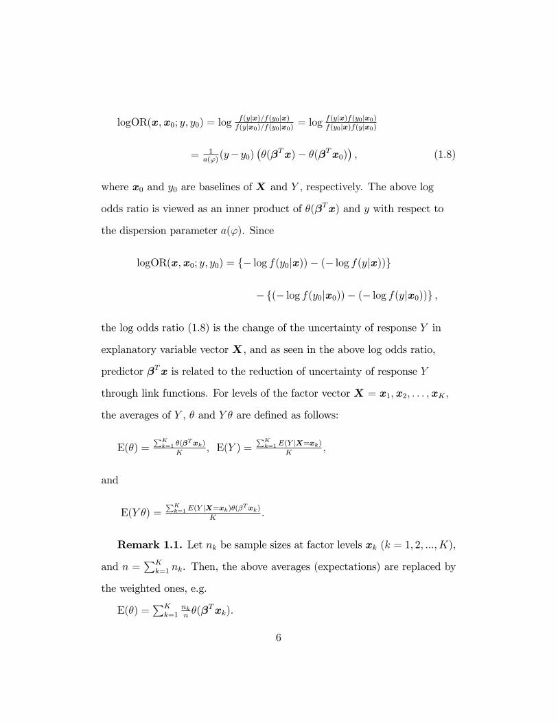
logOR(x;x0; y; y0) = logf(yjx)=f(y0jx)f(yjx0)=f(y0jx0) = log

f(yjx)f(y0jx0)f(y0jx)f(yjx0)

= 1a(')(y�y0)

��(�Tx)� �(�Tx0)

�; (1.8)

where x0 and y0 are baselines of X and Y , respectively. The above log

odds ratio is viewed as an inner product of �(�Tx) and y with respect to

the dispersion parameter a('). Since

logOR(x;x0; y; y0) = f� log f(y0jx))� (� log f(yjx))g

�f(� log f(y0jx0))� (� log f(yjx0))g ;

the log odds ratio (1.8) is the change of the uncertainty of response Y in

explanatory variable vector X, and as seen in the above log odds ratio,

predictor �Tx is related to the reduction of uncertainty of response Y

through link functions. For levels of the factor vector X = x1;x2; : : : ;xK ;

the averages of Y , � and Y � are de�ned as follows:

E(�) =PKk=1 �(�

Txk)

K; E(Y ) =

PKk=1 E(Y jX=xk)

K;

and

E(Y �) =PKk=1 E(Y jX=xk)�(�Txk)

K:

Remark 1.1. Let nk be sample sizes at factor levels xk (k = 1; 2; :::; K),

and n =PK

k=1 nk. Then, the above averages (expectations) are replaced by

the weighted ones, e.g.

E(�) =PK

k=1nkn�(�Txk).

6

When we take the expectation of the inner product (1.8), we have

Cov(�;Y )a(')

+(E(�)��(�Tx0))(E(Y )�y0)

a('),

where Cov(�; Y ) =E(�Y )�E(�)E(Y ): For y0 = E(Y ), the quantity becomes

Cov(�;Y )a(')

(1.9)

and it can be viewed as the average change of uncertainty of response

variable Y in explanatory variable vector X. We have Theorem 1.1 and

Corollary 1.1.

Theorem 1.1. In the GLM with (1.6), the quantity (1.9) is expressed by

the Kullback-Leibler Information:

Cov(�;Y )a(')

=PKk=1 KL(f(y);f(yjxk))

K(1.10)

where f(y) =PKk=1 f(yjxk)

Kand

KL(f(y); f(yjxk)) =Rf(yjxk) log

�f(yjxk)f(y)

�dy +

Rf(y) log

�f(y)

f(yjxk)

�dy

= D (f(yjxk)jjf(y)) +D (f(y)jjf(yjxk))

(k = 1; 2; : : : ; K):

Corollary 1.1. In the GLM with (1.6), the covariance of Y and �(�TX)

is nonnegative, and it is zero if and only if X and Y are independent, i.e.

f(yjxk) = f(y) (k = 1; 2; :::; K).

Example 1.3. An ordinary linear regression model is

Y = �+ �Tx+ e,

7

where e is a normal error with mean 0 and variance �2. Let f(yjx) be a

normal density function with mean � and variance �2. Then, the random

component is

f(yjx) = 1p2��2

exp�� (y��)2

2�2

�= exp

��y� 1

2�2

�2+ �y2

2�2� log

�p2��2

��.

In this expression, setting

� = �, a(') = �2, b(�) = 12�2 and c(y; ') = �y2

2�2� log

�p2��2

�,

and for linear predictor � = �+ �Tx and link function � = �, the normal

linear regression model can be viewed as a GLM.

Example 1.4. Let Y be a binary variable with p = Pr(Y = 1) (= �).

The random component is

f(yjx) = py(1� p)1�y = fp(1� p)�1gy(1� p)

= expny log p

1�p + log(1� p)o.

Then,

� = log p1�p , a(') = 1, b(�) = � log(1� p) and c(y; ') = 0.

Setting link function h(p) = log p1�p , we have the following logistic

regression (logit) model:

8

f(yjx) = exp f(�+ �x)y + log(1� p)g

= expf(�+�x)yg1+exp(�+�x)

.

For the logit model with explanatory variables X1; X2; :::; Xp, the model is

expressed as

f(yjx) = expf(�+Ppi=1 �ixi)yg

1+exp(�+Ppi=1 �ixi)

. (1.11)

�

1.3 Basic Predictive Power Measures for GLMs

In the sense of the previous discussion, it may be appropriate to assess the

predictive or explanatory power of factors based on entropy. In the GLM

framework, predictive power measures are compared, and the advantage of

ECD is mentioned. First, some predictive power measures for regression mod-

els are brie�y discussed. In general regression models, for variation function

D, the predictive power can be measured as follows:

R2D =D(Y )�D(Y jX)

D(Y ), (1.12)

where D (Y ) and D(Y jX) imply a variation function of Y and a conditional

or error variation function given X, respectively (Efron, 1978; Agresti,

1986; Korn & Simon, 1991). Predictive power measures based on the

likelihood function (Theil, 1970; Goodman, 1971) are made according to

powers of the likelihood function, i.e.

R2L = 1��l(0)l(�)

� 2n

,

9

where l (�) is the likelihood function and n is the sample size. Let R be the

multiple correlation coe¢ cient in ordinary linear regression model. The

above measure becomes R2 in ordinary linear regression cases and increases

with model complexity; however it is di¢ cult to interpret the measure in

general (Zhen & Agresti, 2000). The entropy measure (Haberman, 1982)

for categorical responses is based on entropy of Y , H(Y ), and the

conditional entropy H(Y jX), i.e.

R2E =H(Y )�H(Y jX)

H(Y ).

The above measure is included in (1.12). The correlation coe¢ cient of

response Y and its conditional expectation given factor X,

Corr(E (Y jX) ; Y ), is recommended for measuring the predictive power of

GLMs, because the correlation measure can be applied to all types of

GLMs except polytomous response cases (Zheng & Agresti, 2000). This

measure is the correlation coe¢ cient between response Y and the regression

on X, referred to as the regression correlation coe¢ cient.

With respect to entropy, R2L and R2E may be suitable for GLMs. By

considering the average change of log odds ratio, Eshima & Tabata (2007)

proposed the following basic predictive power measure:

mPP (Y jX) � Cov(�;Y )a(')

. (1.13)

The above measure is expressed by the Kullback-Leibler information

(Eshima & Tabata, 2007), and it is increasing in Cov(�; Y ) and decreasing

in a('). Since

10

Var(Y jX = x) = a(')d2b(�)

d�2,

function a(') may be interpreted as the error variation of Y in entropy, i.e.

residual randomness of Y given X. From this, Cov(�; Y ) can be interpreted

as the explained entropy of Y by X. Hence, measure (1.13) is the ratio of

the explained variation of Y for the error variation of Y in entropy.

Entropy variation function DE is de�ned by

DE(Y ) � Cov(�; Y ) + a(').

Since � is a function of X, Cov(�; Y jX) = 0. From this, the conditional

entropy variation of Y given X is

DE(Y jX) � a(').

Considering this, ECD is de�ned as follows:

ECD(X;Y ) = Cov(�;Y )Cov(�;Y )+a(') =

mPP (Y jX)mPP (Y jX)+1

�= DE(Y )�DE(Y jX)

DE(Y )

�. (1.14)

From (1.14), ECD is included in (1.12), and ECD can be viewed as the

proportion of explained variation of Y in entropy. For the normal linear

regression model, it follows that

ECD(X; Y ) = R2.

Let � =��1; �2; :::; �p

�Tbe a regression coe¢ cient vector. For canonical

links � =Pp

i=1 �iXi, ECD (1.14) and the entropy correlation coe¢ cient

(ECC) are decomposed as follows:

11

ECD(X; Y ) =Ppi=1 �iCov(Xi;Y )Pp

i=1 �iCov(Xi;Y )+a('), (1.15)

ECorr(X; Y ) =Ppi=1 �iCov(Xi;Y )pVar(�)

pVar(Y )

:

None of the predictive power measures except ECD and ECC can make

the above type of decomposition for GLMs with canonical links. In addition

to the desirable properties of measures for GLMs, (i) to (v), decomposability

such as (1.15) may also be a suitable property for a predictive power mea-

sure, because the relative importance of Xi may be assessed by �iCov(Xi; Y ).

Moreover, ECD is scale-invariant in GLMs with multivariate responses; how-

ever ECC is not. In this respect, ECD is superior to ECC.

Table 1.1 Properties of �ve predictive power measures in GLMs

Property Corr(E (Y jX) ; Y ) R2L R2E ECC ECD

(i) interpretability �

(ii) R or R2 �

(iii) entropy �

(iv) all GLMs �

(v) monotonicity 4 4

(vi) decomposition � � �

Table 1.1 summarizes the properties of the �ve measures mentioned above.

Measures Corr(E (Y jX) ; Y ) and ECorr(X; Y )may have property (v) in most

of cases; however it is not easy to prove the property in general. From this

table, ECD(X;Y ) is the most desirable predictive power measure for GLMs.

12

Example 1.5. Let X and Y be p and q dimensional random vectors,

respectively; and the joint distribution is assumed to be a (p + q)�variate

normal distribution with the following covariance matrix:

� =

0B@ �XX �XY

�Y X �Y Y

1CA.Let the inverse of the above matrix be denoted by

��1 =

0B@ �XX �XY

�Y X �Y Y

1CA.Then, � = �Y XX and a(') = 1, so we have

mPP (Y jX) = tr�Y X�XY .

From this,

ECD(X; Y ) = tr�Y X�XYtr�Y X�XY +1

.

Let �i (i = 1; 2; :::;minfp; qg) be the squared canonical correlation

coe¢ cients. Then,

ECD(X; Y ) =Pminfp;qgi=1

�i1��iPminfp;qg

i=1�i

1��i+1.

For q = 1, ECD is reduced to the usual coe¢ cient of determination

�1 (= R2). �

Example 1.6. In the logistic regression model (1.11), we have

ECD(X; Y ) =Ppi=1 �iCov(Xi;Y )Pp

i=1 �iCov(Xi;Y )+1.

�

13

2 Application of ECD

2.1 Asymptotic Property of the ML Estimator of ECD

Let f(y) and g (x) be the marginal density or probability function of Y and

X, respectively. Then, the association measure is expressed as

mPP (Y jX) =RRf(yjx)g(x) log

�f(yjx)f(y)

�dxdy

+RRf(y)g(x) log

�f(y)f(yjx)

�dxdy. (2:1)

If Y is discrete, the integral is replaced with the summation. If X is not

random and take values xk (k = 1; 2; :::; K), the above measure can be

modi�ed as follows:

mPP (Y jX)

=PK

k=1nkn

�Rf(yjxk) log

�f(yjxk)f(y)

�dy +

Rf(y) log

�f(y)

f(yjxk)

�dy�, (2:2)

where nk are sample sizes at levels xk (k = 1; 2; :::; K), and n =PK

k=1 nk.

We have the following theorem.

Theorem 2.1. Let[mPP (Y jX), bf(yjxk), and bf(y) be the ML estimatorsof mPP (Y jX), f(yjxk), and f(y), respectively. If the null model, i.e. � = 0,

holds, the ML estimator of (2.2) multiplied by sample size n, i.e.

n�[mPP (Y jX)

=PK

k=1 nk

�R bf(yjxk) log � bf(yjxk)bf(y)�dy +

R bf(y) log � bf(y)bf(yjxk)�dy�,

is asymptotically distributed according to the chi-square distribution with

degrees of freedom p as the sample sizes ni tend to in�nity.

14

Proof. For simplicity of the discussion, the theorem is proven in the case

where Y is a polytomous variable with levels or categories f1; 2; : : : ; Jg. Let

�jjk = Pr (Y = jjX = xk) and �j = Pr (Y = j); and let b�jjk and b�j be theML estimators of the �jjk and �j, respectively. Under the null hypothesis

and for su¢ ciently large nk, we have

n�[mPP (Y jX) =PK

k=1 nkPJ

j=1

nb�jjk log b�jjkb�j + b�j log b�jb�jjko

=PK

k=1

PJj=1

(nkb�jjk�nkb�j)22nkb�jjk +

PKk=1

PJj=1

(nkb�jjk�nkb�j)22nkb�j + o(n)

=PK

k=1

PJj=1

(nkb�jjk�nkb�j)2nkb�jjk + o(n),

where

o(n)n

P�! 0 (n �!1) :

Hence, the theorem follows. �

When the explanatory variables X are random, the following theorem

holds similarly.

Theorem 2.2. If the null model, i.e. � = 0, holds, the ML estimator of

(2.1) multiplied by sample size n, i.e.

n�[mPP (Y jX)

= n��RR bf(yjx)bg(x) log � bf(yjx)bf(y)

�dxdy +

RR bf(y)bg(x) log � bf(y)bf(yjx)�dxdy

�is asymptotically distributed according to the chi-square distribution with

degrees of freedom p as the sample size n tends to in�nity.

15

Since

ECD(X;Y ) = Cov(�;Y )=a(')Cov(�;Y )=a(')+1 =

mPP (Y jX)mPP (Y jX)+1 ,

the ML estimator of ECD(X;Y ) is

[ECD(X;Y ) = [mPP (Y jX)[mPP (Y jX)+1

.

From this, we can test the hypothesis ECD(X; Y ) = 0 based on the

following statistic:

�2 = n�[mPP (Y jX)�= n

dCov(�;Y )a(b')

�. (2.3)

The above statistic is asymptotically distributed according to a non-central

chi square distribution with non-centrality

� = n�mPP (Y jX)

and degrees of freedom p. Let

c = 1 + �p+�

and � 0 = p+ �2

p+2�.

Statistic �2

cis asymptotically distributed according to the chi square

distribution with degrees of freedom � 0. As � 0 becomes large, the chi square

distribution tends to a normal distribution with mean � 0 and variance 2� 0.

From this, for su¢ ciently large sample size n, statistic (2.3)

16

�2

n= mPP (Y jX)

is asymptotically normally distributed with mean c�0

nand variance 2c2�0

n2

(Patnaik, 1949). For su¢ ciently large n, we have

c�0

n� mPP (Y jX),

2c2�0

n2� 2c

nmPP (Y jX).

From this, the asymptotic standard error (ASE) of[mPP (Y jX) isq2cn[mPP (Y jX).

Example 2.1. Agresti (2002, pp. 247-250) analyzed the beetle mortality

data with complementary log-log model, in which beetles were exposed to

gaseous carbon disul�de at various concentrations, and the numbers of beetles

killed after the 5-hour-exposure were observed (Table 2.1). Let X be gaseous

carbon disul�de concentration, and � and � the model parameters. Then,

for the complementary log-log link we have

� = log�1�expf� exp(�+�x)gexpf� exp(�+�x)g

�:

For the maximum likelihood estimates � = �39:52 (ASE = 3:23) and

� = 22:01 (ASE = 1:80), ECD is calculated as

ECD = 0:475 (ASE = 0:024):

The ECD indicates that 47:5% of variation of response variable Y in

entropy is explained by the gaseous carbon disul�de concentration X.

17

Table 2.1. Beetles Killed after Exposure to Carbon Disul�de

Log Dose No. of Beetles No. of Beetles Killed

1:691 60 6

1:724 60 13

1:755 62 18

1:784 56 28

1:811 63 52

1:837 59 53

1:861 62 61

1:884 60 60

�

2.2 GLMs with canonical links

Most regression analyses with GLMs are performed using canonical links.

Let X = (X1; X2; :::; Xp)T be a p � 1 factor or explanatory variable vector;

let Y be a response variable; let � =��1; �2; :::; �p

�Tbe a regression para-

meter vector; and let � =Pp

i=1 �iXi be the canonical links. Then, ECD is

decomposed as

ECD(X; Y ) =Ppi=1 �iCov(Xi;Y )Pp

j=1 �jCov(Xj ;Y )+a('). (2.4)

The above decomposition consists of components that relate to regression

coe¢ cients �i, and the contribution of Xi on Y may be de�ned by using

18

�iCov(Xi; Y ).

If Xi are independent or the experimental design is a multiway layout

experiment, the contribution ratio of Xi on the response is de�ned by

CR (Xi) =�iCov(Xi;Y )Pp

k=1 �kCov(Xk;Y ).

In general, Xi are correlated or the experiment model has higher-order

interactions. Then, the contribution ratio of Xi is de�ned by

CR (Xi) =Cov(�;Y )�Cov(�;Y jXi)

Cov(�;Y ).

Example 2.2. The present discussion is applied to the ordinary two-

way layout experimental design model. Let X1 and X2 be factors with levels

f1; 2; : : : ; Ig and f1; 2; : : : ; Jg, respectively. Then, the linear predictor is a

function of (X1; X2) = (i; j), i.e.

� = �i + �j + (��)ij.

For model identi�cation, the following constraints are placed on these

parameters:

PIi=1 �i =

PJj=1 �j =

PIi=1(��)ij =

PJj=1(��)ij = 0.

Let

Xki =

8><>: 1 (Xk = i)

0 (Xk 6= i)(k = 1; 2):

Then, dummy vectors

19

X1 = (X11; X12; : : : ; X1I)T and X2 = (X21; X22; : : : ; X2J)

T

are identi�ed with factors X1 and X2, respectively. From this, the

systematic component of the above model can be written as follows:

� = �TX1 + �TX2 +

TX1 X2;

where

� = (�1; �2; : : : ; �I)T , � = (�1; �2; : : : ; �J)

T ,

= ((��)11; (��)12; : : : ; (��)1J ; : : : ; (��)IJ)T ,

and

X1 X2 = (X11X21;X11X22; : : : ; X11X2J ; : : : ; X1IX2J)T .

Let Cov(X1; Y ), Cov(X2; Y ) and Cov(X1 X2; Y ) are covariance

matrices. Then the total e¤ect of X1 and X2 is

mPP (Y j (X1;X2)) =Cov(�;Y )

�2

= tr�TCov(X1;Y )�2

+ tr�TCov(X2;Y )�2

+ tr TCov(X1X2;Y )�2

=1I

PIi=1 �

2i

�2+

1J

PJj=1 �

2j

�2+

1IJ

PJj=1

PIi=1(��)

2ij

�2.

The above three terms are referred to as the main e¤ect of X1, that of X2

and the interactive e¤ect, respectively. Then, ECD is calculated as follows:

ECD((X1;X2) ; Y ) =1I

PIi=1 �

2i+

1J

PJj=1 �

2j+

1IJ

PJj=1

PIi=1(��)

2ij

1I

PIi=1 �

2i+

1J

PJj=1 �

2j+

1IJ

PJj=1

PIi=1(��)

2ij+�

2.

In this case,

20

CR (X1) =Cov(�;Y )�Cov(�;Y jXi)

Cov(�;Y )=

1I

PIi=1 �

2i

Cov(�;Y ),

CR (X2) =Cov(�;Y )�Cov(�;Y jXi)

Cov(�;Y )=

1J

PJj=1 �

2j

Cov(�;Y ).

The rest

1� CR (X1)� CR (X2) =1IJ

PJj=1

PIi=1(��)

2ij

Cov(�;Y )

is due to the e¤ect of the interaction.

Table 2.2. Length of Home Visit in minutes by Public Health Nurses by

Nurse�s Age Group and Type of Patient

Factor X2 (nurse�s age group) (years old)

Factor X1

(Type of Patients)

1 2 3 4

(20 to 29) (30 to 39) (40 to 49) (50 and over)

1 (Cardiac)20 25 22

27 21

25 30 29

28 30

24 28 24

5 30

28 31 26

29 32

2 (Cancer)30 45 30

35 36

30 29 31

30 30

39 42 36

42 40

40 45 50

45 60

3 (C.V.A)31 30 40

35 30

32 35 30

40 30

41 45 40

40 35

42 50 40

55 45

4 (Tuberculosis)20 21 20

20 19

23 25 28

30 31

24 25 30

26 23

29 30 28

27 30

21

Table 2.2 shows two-way layout experiment data in a study of length of

time spent on individual home visits by public health nurses (Daniel (1999),

pp. 348-353). In the example, analysis of the e¤ects of factors, i.e. the type

of patient and the age of a nurse, on the nurses�behavior will be signi�cant.

Let Y be length of home visit, and let factors X1 and X2 denote the type

of a patient and the age of a nurse, respectively. The results of two-way

analysis of variance are shown in Table 2.3. The main and interactive e¤ects

of factors are signi�cant. In this case, levels of factor vector X = (X1; X2)

are (i; j) (i = 1; 2; 3; 4; 5; j = 1; 2; 3; 4; 5). Although factors X1 and X2 are

independent (orthogonal), the model has interaction terms between them.

By using the present approach, the variance decomposition in Table 2.3 we

have

ECD((X1;X2) ; Y ) =3226:45+1185:05+704:45

6423:55= 0:796 (SE = 0:018).

From this, 79.6% of entropy is explained by the two variables (factors). The

contributions of the factors are calculated as follows:

CR (X1) =3226:456423:55

= 0:502 and CR (X2) =1185:056423:55

= 0:184 .

The contribution of X1 on Y is about three times greater than that of X2.

22

Table 2.3. Analysis of variance of length of time

spent on individual home visits by public health nurses

Source SS df MS F p

X1 3226:45 3 1075: 5 52: 641 0:000

X2 1185:05 3 395: 02 19: 334 0:000

(X1X2) 704:45 9 78: 272 3: 831 0:000

Residual 1307:6 64 20: 431 �

Total 6423:55 79 � �

Example 2.3. Table 2.4 shows death penalty data to study the e¤ects of

defendant�s and victim�s racial characteristics on whether persons convicted

homicide received the death penalty (Agresti, pp. 48-49), and the data were

analyzed with the following logit model

f(yjx) = expf(�+�dxd+�vxv)yg1+exp(�+�dxd+�vxv)

,

where Xd and Xv imply the defendant�s and victim�s race, i.e. 0= black

and 1=white; the response death penalty Y takes the value 0=no or 1=yes.

The estimated parameters were b� = �3:596 (SE=0.507), b�d = �0:868(SE=0.367) and b�v = 2:404 (SE=0.601) (Agresti, p. 201). From the results,

the odds of death penalty for the white defendant given the victim�s race is

exp (�0:868) = 0:420 times higher than that for the black defendant, and

the odds of death penalty for the white victim given the defendant�s race is

exp (2:404) = 11: 067 times higher than that for black victim. Since the

23

predictive power measured with ECD is ECD = 0:036 (SE = 0:014), the

e¤ects of the defendant�s and victim�s races on the death penalty are small.

The contribution ratios of the explanatory variables on the response are

calculated according to (2.4) as follows:

CR (Xd) = 0:603 and CR (Xv) = 0:813:

Table 2.4. Death Penalty Data

Victims�Race Defendant�s RaceDeath Penalty

Yes No

White White 53 414

Black 11 37

Black White 0 16

Black 4 139

2.3 Application to a generalized logit model

A baseline-category logit model is considered. Let X1 and X2 be categorical

factors that take levels f1; 2; : : : ; Ig and f1; 2; : : : ; Jg, respectively, and let Y

be a categorical response variable with levels f1; 2; : : : ; Kg. Let

Xai =

8><>: 1 (Xa = i)

0 (Xa 6= i)(a = 1; 2) and Yk =

8><>: 1 (Y = k)

0 (Y 6= k). (2.5)

Then, dummy variable vectors

24

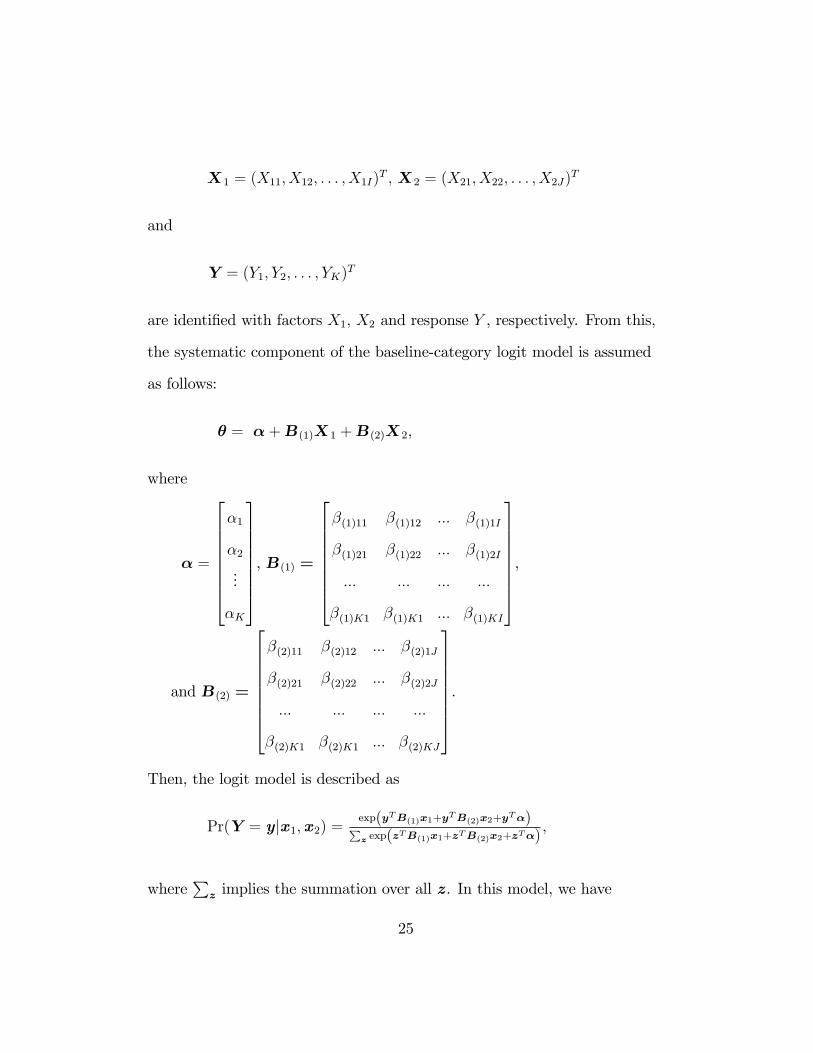
X1 = (X11; X12; : : : ; X1I)T ; X2 = (X21; X22; : : : ; X2J)

T

and

Y = (Y1; Y2; : : : ; YK)T

are identi�ed with factors X1; X2 and response Y , respectively. From this,

the systematic component of the baseline-category logit model is assumed

as follows:

� = �+B(1)X1 +B(2)X2;

where

� =

266666664

�1

�2...

�K

377777775, B(1) =

266666664

�(1)11 �(1)12 ::: �(1)1I

�(1)21 �(1)22 ::: �(1)2I

::: ::: ::: :::

�(1)K1 �(1)K1 ::: �(1)KI

377777775,

and B(2) =

266666664

�(2)11 �(2)12 ::: �(2)1J

�(2)21 �(2)22 ::: �(2)2J

::: ::: ::: :::

�(2)K1 �(2)K1 ::: �(2)KJ

377777775.

Then, the logit model is described as

Pr(Y = yjx1;x2) =exp(yTB(1)x1+y

TB(2)x2+yT�)P

z exp(zTB(1)x1+zTB(2)x2+z

T�);

whereP

z implies the summation over all z. In this model, we have

25

ECD(X; Y ) =trB(1)Cov(X1;Y )+ trB(2)Cov(X2;Y )

trB(1)Cov(X1;Y )+ trB(2)Cov(X2;Y )+1.

In the following example, the ECD approach is demonstrated.

Example 2.4. The data for an investigation of factors in�uencing the

primary food choice of alligators (Table 2.5) are analyzed (Agresti, 2002;

pp. 268-271). In this example, explanatory variables are X1: lakes where

alligators live, {1. Hancock, 2. Oklawaha, 3. Tra¤ord, 4. George}; and

X2: sizes of alligators, {1. Small, 2. Large}; and the response variable is Y :

primary food choice of alligators, {1. Fish, 2. Invertebrate, 3. Reptile, 4.

Bird, 5. Other}. In this analysis, the generalized logit model described in

this section is used, and we set I = 4, J = 2, and K = 5 in (2.5). From this

model the following estimates of regression coe¢ cients are obtained (Agresti,

2002; pp. 268-271):

bB1 =

266666666664

�0:826 �0:006 �1:516 0

�2:485 0:931 �0:394 0

0:417 2:454 1:419 0

�0:131 �0:659 �0:429 0

0 0 0 0

377777777775and bB2 =

266666666664

�0:332 0

1:127 0

�0:683 0

�0:962 0

0 0

377777777775:

By using the above estimates, we have

tr bB1\Cov (X1; Y ) = 0:258 and tr bB2

\Cov (X2; Y ) = 0:107.

219�[mPP (Y jX1; X2) = 219� (0:258 + 0:107)

= 79: 935 (df = 16; P = 0:000).

26

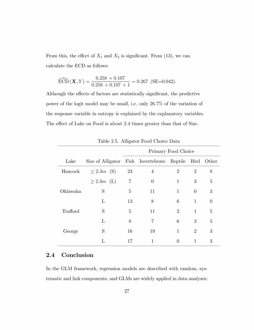
From this, the e¤ect of X1 and X2 is signi�cant. From (13), we can

calculate the ECD as follows:

[ECD (X; Y ) =0:258 + 0:107

0:258 + 0:107 + 1= 0:267 (SE=0.042):

Although the e¤ects of factors are statistically signi�cant, the predictive

power of the logit model may be small, i.e. only 26:7% of the variation of

the response variable in entropy is explained by the explanatory variables.

The e¤ect of Lake on Food is about 2:4 times greater than that of Size.

Table 2.5. Alligator Food Choice Data

Primary Food Choice

Lake Size of Alligator Fish Invertebrate Reptile Bird Other

Hancock � 2:3m (S) 23 4 2 2 8

� 2:3m (L) 7 0 1 3 5

Oklawaha S 5 11 1 0 3

L 13 8 6 1 0

Tra¤ord S 5 11 2 1 5

L 8 7 6 3 5

George S 16 19 1 2 3

L 17 1 0 1 3

2.4 Conclusion

In the GLM framework, regression models are described with random, sys-

tematic and link components, and GLMs are widely applied in data analyses;

27

however the explanatory powers of GLMs have not been measured in practical

data analyses except the ordinary linear regression model. In this seminar,

GLMs are discussed from a view point of entropy, and ECD for measuring

explanatory or predictive power of GLMs has been introduced and the utility

of ECD has been shown for practical data analyses.

Acknowledgement 1 The author would like to thank Prof. Claudio Bor-

roni and all the members of Department of Quantitative Methods for Eco-

nomics and Business Sciences, the University of Milan (Universita degli Studi

di Milano) for giving me a valuable opportunity to make the present seminar.

References

[1] Agresti, A. (1986). Applying R2-type measures to ordered categorical

data, Technometrics; 28: 133-138.

[2] Agresti, A. (2002). Categorical Data Analysis, Second Edition, John

Wiley & Sons, Inc.: New York.

[3] Ash, A. & Shwarts, M. (1999). R2: A useful measure of model perfor-

mance with predicting a dichotomous outcome, Statistics in Medicine;

18: 375-384.

[4] Daniel, W. W. (1999). Biostatistics: A Foundation for Analysis in the

Health Sciences, Seventh Edition, John Wiley & Sons, Inc.: New York.

28

[5] Efron, B. (1978). Regression and ANOVA with zero-one data: measures

of residual variation, Journal of the American Statistical Association;

73: 113-121.

[6] Eshima, N. & Tabata, M. (2007). Entropy correlation coe¢ cient for

measuring predictive power of generalized linear models, Statistics and

Probability Letters; 77, 588-593.

[7] Eshima, N & Tabata, M. (2010). Entropy coe¢ cient of determination for

generalized linear models, Computational Statistics and Data Analysis,

54, 1381-1389, 2010.

[8] Eshima, N & Tabata, M. (2011). Three predictive power measures for

generalized linear models: Entropy coe¢ cient of determination, entropy

correlation coe¢ cient and regression correlation coe¢ cient, Computa-

tional Statistics and Data Analysis, 55, 3049-3058.

[9] Goodman, L. A. (1971). The analysis of multinomial contingency tables:

stepwise procedures and direct estimation methods for building models

for multiple classi�cations, Technometrics; 13: 33-61.

[10] Haberman, S. J. (1982). Analysis of dispersion of multinomial responses,

Journal of the American Statistical Association; 77: 568-580.

[11] Kent, J. T. (1983). Information gain and a general measure of correla-

tion, Biometrika, 70, 163-173.

29

[12] Korn, E. L. and Simon, R. (1991). Explained residual variation, ex-

plained risk and goodness of �t, American Statistician; 45: 201-206.

[13] McCullagh, P. and Nelder, J. A. (1989). Generalized Linear models, 2nd

Ed. Chapman and Hall: London.

[14] Mittlebock, M. and Schemper, M. (1996). Explained variation for logistic

regression, Statistics in Medicine; 15: 1987-1997.

[15] Nelder, J. A. and Wedderburn, R. W. M. (1972). Generalized linear

model, Journal of the Royal Statistical Society A; 135: 370-384.

[16] Patnaik, P.B. (1949). The non-central �2 and F-distributions and their

applications, Biometrika, 36, 202-232.

[17] Theil, H. (1970). On the estimation of relationships involving qualitative

variables, American Journal of Sociology; 76: 103-154.

[18] Zheng, B. and Agresti, A. (2000). Summarizing the predictive power of

a generalized linear model, Statistics in Medicine 2000; 19: 1771-1781.

30