ensemble evaluation of hydrologically enhanced noah-lsm

Ensemble Evaluation of Hydrologically Enhanced Noah-LSM: Partitioning of theWater Balance in High-Resolution Simulations over the Little Washita River

Experimental Watershed

ENRIQUE ROSERO,* LINDSEY E. GULDEN,* AND ZONG-LIANG YANG

Department of Geological Sciences, Jackson School of Geosciences, The University of Texas at Austin, Austin, Texas

LUIS G. DE GONCALVES

NASA Goddard Space Flight Center, Hydrological Sciences Branch, Greenbelt, and Maryland Earth System Science

Interdisciplinary Center, University of Maryland, College Park, College Park, Maryland

GUO-YUE NIU

Biosphere2 Earthscience, The University of Arizona, Tucson, Arizona

YASIR H. KAHEIL

International Research Institute for Climate and Society, Columbia University, Palisades, New York

(Manuscript received 23 October 2009, in final form 6 August 2010)

ABSTRACT

The ability of two versions of the Noah land surface model (LSM) to simulate the water cycle of the Little

Washita River experimental watershed is evaluated. One version that uses the standard hydrological param-

eterizations of Noah 2.7 (STD) is compared another version that replaces STD’s subsurface hydrology with

a simple aquifer model and topography-related surface and subsurface runoff parameterizations (GW). Sim-

ulations on a distributed grid at fine resolution are compared to the long-term distribution of observed daily-

mean runoff, the spatial statistics of observed soil moisture, and locally observed latent heat flux. The evaluation

targets the typical behavior of ensembles of models that use realistic, near-optimal sets of parameters important

to runoff. STD and GW overestimate the ratio of runoff to evapotranspiration. In the subset of STD and GW

runs that best reproduce the timing and the volume of streamflow, the surface-to-subsurface runoff ratio is

overestimated and simulated streamflow is much flashier than observations. Both models’ soil columns wet and

dry too quickly, implying that there are structural shortcomings in the formulation of STD that cannot be

overcome by adding GW’s increased complexity to the model. In its current formulation, GW extremely un-

derestimates baseflow’s contribution to total runoff and requires a shallow water table to function realistically.

In the catchment (depth to water table .10 m), GW functions as a simple bucket model. Because model

parameters are likely scale and site dependent, the need for even ‘‘physically based’’ models to be extensively

calibrated for all domains on which they are applied is underscored.

1. Introduction

Among the components of the water balance, runoff

has arguably the greatest importance for society. The

Intergovernmental Panel on Climate Change (IPCC)

identified the vulnerability of freshwater resources to

climate change and highlighted the need for increased

capacity to model runoff processes at high-resolution

(catchment scale) within the land surface models (LSMs)

that are linked to climate models (Bates et al. 2008).

Such improvements, combined with more extensive, high-

resolution runoff datasets, are necessary to better assess

the feedbacks affecting freshwater resources. Runoff,

together with soil moisture, is in general poorly rep-

resented in LSMs (Viterbo 2002; Nijseen and Bastidas

* Current affiliation: ExxonMobil Upstream Research Com-

pany, Houston, Texas.

Corresponding author address: Zong-Liang Yang, 1 University Sta-

tion C1100, The University of Texas at Austin, Austin, TX 78712-0254.

E-mail: [email protected]

FEBRUARY 2011 R O S E R O E T A L . 45

DOI: 10.1175/2010JHM1228.1

� 2011 American Meteorological Society

2005; Overgaard et al. 2006). Major uncertainty re-

mains in LSMs’ simulation of the surface water bal-

ance. Some of this uncertainty is governed by the

parameterization of processes that drive runoff and the

differences in the storage characteristics of LSMs

(Wetzel et al. 1996; Pitman 2003). The strong interac-

tion between the water and energy balances means that

systematic errors in the allocation of moisture to reser-

voirs and runoff propagate to the partitioning of turbu-

lent heat fluxes (Chen et al. 1997; Koster and Milly 1997;

Liang et al. 1998; Wood et al. 1998; Dirmeyer 2006), which

affects the simulation of weather and climate (Pitman

et al. 1999; Li et al. 2007).

The complexity of the subsurface hydrology parame-

terizations in LSMs is relatively low when compared to

the complexity of their parameterizations of above-

ground processes (Stockli et al. 2008). While most LSMs

describe the canopy and root zone in great detail, the

interactions between groundwater, the root zone, and

surface water are usually neglected (Overgaard et al. 2006).

Because of the lack of observations of water movement in

the vadose zone, diverse representations of infiltration,

drainage, and interflow processes in LSMs stem mainly

from their unconstrained development, which focused

primarily on regional fluxes to the atmosphere (Wetzel

et al. 1996). Many LSMs, like the Noah LSM (Ek et al.

2003), neglect topographic effects, assume spatially con-

tinuous soil moisture values, parameterize surface runoff

with a simple infiltration-excess scheme, and treat base-

flow as a linear function of bottom soil-layer drainage

(Schaake et al. 1996). More complex in its subsurface hy-

drology parameterizations than most LSMs, the multi-

level reservoir Variable Infiltration Capacity (VIC) (Wood

et al. 1992) family of models and its descendants (e.g.,

Liang et al. 1996) use a spatial probability distribution to

represent subgrid heterogeneity in soil moisture and treat

baseflow as a nonlinear recession curve. Alternative LSM

runoff schemes such as the Catchment model (Koster et al.

2000; Ducharne et al. 2000) have been used only in lim-

ited research applications (e.g., Reichle and Koster 2005).

Lately, groundwater dynamics have been incorporated

into LSMs (e.g., Gutowski et al. 2002; Liang et al. 2003;

Yeh and Eltahir 2005; Maxwell and Miller 2005; Niu

et al. 2007; Fan et al. 2007; Kollet and Maxwell 2008).

Major concerted efforts to evaluate the ability of mul-

tiple LSMs to simulate runoff at coarse scales in temperate

regions indicate that 1) bucket models are insufficiently

complex to capture runoff processes (Wood et al. 1998;

Lohmann et al. 1998). 2) Especially in semiarid regions,

most LSMs overestimate mean annual runoff [and

hence underestimate evapotranspiration (ET)] and that

the overestimation of runoff is especially pronounced dur-

ing summer and in the drier portions of the basin (Wood

et al. 1998; Lohmann et al. 1998). 3) Models whose run-

off schemes were dominated by subsurface runoff (base-

flow) most accurately simulated summer-season runoff

(Lohmann et al. 1998). 4) Most LSMs can simulate monthly

total river runoff relatively well, provided that the pre-

cipitation and other forcing input data are sufficiently

accurate (Oki et al. 1999). Performance degrades sig-

nificantly when evaluated at a daily time scale, although

most LSMS are still able to slightly outperform the mean

discharge (Boone et al. 2004). 5) Increasing model grid

resolution tends to increase the volume of simulated

runoff (Boone et al. 2004), which implies that there may

be a need for the revision of modeling formulations as

increasingly finely gridded models and/or at catchment-

based models are used. 6) Model efficiency in the sub-

basins was found to be lower than the model efficiency

for the entire watershed. 7) LSMs appear to be sensitive

to subgrid runoff parameterizations (Stockli et al. 2007)

and model parameters (Wood et al. 1998). 8) With ap-

propriate automatic calibration of a large number of pa-

rameters and with the introduction of correction factors

for the model forcing (precipitation and incoming radi-

ation), LSMs can simulate runoff at 1/88 with accuracy

comparable to that of the conceptual hydrological models

participating in the Model Parameter Estimation Experi-

ment (MOPEX) (Nasonova et al. 2009).

The multimodel intercomparisons’ use of only one or

a few model realizations, however, has made it difficult

to definitively attribute the sensitivity of runoff simula-

tions to parameterization, to parameters, or to a combi-

nation of the two. The identification and evaluation of

distributed hydrological models is complicated by the

large number of model parameters and the lack of suf-

ficiently powerful methods that can be used to perform

a truly distributed assessment of model performance

(e.g., Beven 1989, 2001, 2002; Konikow and Bredehoeft

1992; Refsgaard 1997; Refsgaard and Henriksen 2004).

We attempt such a comparison here.

We evaluate the ability of two versions of the Noah

LSM to simulate the water cycle at high spatial and

temporal resolution without the use of forcing-correction

factors. The runoff parameterization of the standard re-

lease 2.71 of the Noah LSM (STD) is compared against

a version of the Noah LSM that has been augmented with

a lumped, unconfined aquifer model (GW). GW repre-

sents the vertical flow of water between the soil column

and an aquifer according to a parameterization of Darcy’s

Law. In an effort to capture the subgrid heterogeneity in

land surface properties that controls runoff generation,

a TOPMODEL-based parameterization (Niu et al. 2005,

2007) replaces in GW the surface and subsurface runoff

parameterizations of STD. We hypothesize that because of

GW’s increased complexity and conceptual realism when

46 J O U R N A L O F H Y D R O M E T E O R O L O G Y VOLUME 12

compared to STD, and because of GW’s good perfor-

mance in reproducing near-surface fluxes and states at

single points in semihumid regions of transition zones

(Rosero et al. 2009, 2010), GW will outperform STD when

simulating runoff.

We address the following broad questions: Can a

medium-complexity LSM (i.e., Noah STD) simulate run-

off at a fine spatial and temporal resolution in a zone of

transition between humid and arid climates? Does the

addition of a more complex, physically realistic param-

eterization of groundwater dynamics and topography-

based runoff improve the model’s capacity to simulate

runoff? Note that we do not expect the LSMs to be able

to provide highly accurate mean daily discharge pre-

dictions; rather, we evaluate them based on their capacity

to reproduce the essential components and character

of runoff generation and of the water balance. We use

an extensive evaluation approach that incorporates

the models’ typical behavior (i.e., their ‘‘signatures’’) of

ensembles that use realistic, near-optimal sets of param-

eters (Rosero et al. 2009, 2010). We focus extensively on

a set of Monte Carlo–derived behavioral runs that best

reproduce the timing and the volume of streamflow.

Our chosen modeling domain is the Little Washita

River Experimental Watershed (LWREW; Allen and

Naney 1991) (Fig. 1). Noting the community’s call for

increased spatial and temporal scales when predicting

runoff, we run both versions of Noah LSM on a 4-km

grid and evaluate daily river discharge. We further assess

the models’ abilities to simultaneously simulate runoff,

soil moisture, and evapotranspiration. This analysis is at

a finer temporal and spatial scale than has been done

previously for LSMs.

This is a preliminary study aimed toward improved

runoff simulation within LSMs. Because of the small

scale of the basin we assume routing is not necessary to

predict daily total streamflow volumes (Fig. 2). We further

assume that the meteorological input forcing data are

accurate enough (i.e., no correction is required, Fig. 3).

Section 2 introduces the models, evaluation datasets,

and Monte Carlo–based methods. Section 3 presents the

results of the intercomparison. Discussion of our con-

clusions is offered in section 4.

2. Data, models, and methods

We used two versions of the Noah LSM (Ek et al.

2003; Mitchell et al. 2004) to produce ensembles of LSM

realizations of near-surface states and fluxes over the

Little Washita basin in Oklahoma from 1 January 1997

to 31 December 2007. The first five years of model

output are treated as spinup. We evaluate simulations of

the period 1 January 2002 to 31 December 2007.

a. The Little Washita River Experimental Watershed

The LWREW (Fig. 1), a tributary of the Washita

River, is just south of 358N and is centered on 2988E.

Grass, crops, and wooded grassland cover the 611-km2

basin, which contains soil types ranging from fine sand

to silty loam. The climate is temperate and continental:

FIG. 1. LWREW modeling domain. (a) Hydrography and loca-

tions of the USGS streamflow gauges, ARS soil moisture obser-

vation sites, and the FLUXNET tower. (b) 1-km FAO/STATSGO

soil texture data. (c) 1-km UMD vegetation type data. (d) Groups

A–G of cells with the same vegetation and soil types on the 4-km

modeling domain used in all model realizations described here.

Note the delineation of 3 subbasins: upstream (7327442), mid-

catchment (7327447), and downstream at the outlet (7327550). See

Table 1 for soil and vegetation classification.


average annual rainfall is 760 mm. Most precipitation is

received in the spring and fall. Summers are long, hot,

and dry; winters are short, temperate, and dry. Mean

annual temperature is 168C. Daily-mean maximum (min-

imum) temperature in July is 358C (218C), and daily-mean

maximum (minimum) temperature in January is 108C

(248C). The influence of snow processes and frozen soil

hydrology is negligible. The watershed is well drained,

with gently rolling hills dominating the landscape. Max-

imum topographic relief is about 180 m. The LWREW is

slow draining: baseflow is a major component of over-

all runoff, which makes the basin an ideal location in

which to test the parameterizations of GW. Additional

description of the watershed can be found in Allen and

Naney (1991).

b. The Noah LSM

Noah is a medium-complexity LSM that takes mete-

orological forcing as input and uses physically based

equations to simulate near-surface states and surface-to-

atmosphere fluxes. Noah is used operationally by the

National Centers for Environmental Prediction models

and it is the land component of the Weather Research

Forecasting model. Noah uses mass conservation and

a diffusive form of the Richards equation to represent

vertical water flow through its four-layer soil column

(with lower boundaries at 0.1, 0.4, 1.0, and 2.0 m). The

dependency of hydraulic conductivity and soil matric

potential on soil moisture is parameterized according to

Clapp and Hornberger (1978).

The two versions of Noah that we used are hydro-

logically distinct: 1) in STD, the standard hydrological

parameterizations of Noah release 2.71 are used; 2) in

GW, a simple aquifer model is coupled to the model’s soil

columns and the surface and subsurface runoff parame-

terizations of STD are replaced by the TOPMODEL-

based parameterizations of Niu et al. (2005, 2007).

Because the maximum time-lag correlation of daily

streamflow between gauges upstream of the outlet is

under 1 day, no routing scheme was used (Fig. 2), and the

hourly runoff was simply aggregated downstream daily.

1) THE STANDARD VERSION OF THE NOAH

LSM (STD)

STD uses an infiltration-excess parameterization to

represent surface runoff and a gravitational drainage pa-

rameterization to represent subsurface runoff (Schaake

et al. 1996). Surface runoff (Qs) is

Qs5 P

d� Inf

max, (1)

where Pd is the rate at which water reaches the soil surface

and Infmax is the maximum rate of infiltration into the soil.

Here Infmax is calculated as function of the hydraulic

conductivity of the first soil layer, according to the subgrid

parameterization of the water balance deficit as

Infmax

5 Pd

Dx[1� exp(�kdt 3 d

t)]

Pd

1 Dx[1� exp(�kdt 3 d

t)]

, (2)

where Dx is the soil moisture (u) deficit term integrated

across soil layers (Dzi) on time interval dt:

Dx

5 �4

i51Dz

i(u

sat� u

i), (3)

and the variable kdt is calculated as a function of the

parameter kdtref and the ratio of the saturated hydraulic

conductivity (Ksat) and its reference value (Kref):

FIG. 2. Lag-correlation coefficients between streamflow at the

outlet gauge (07327550) and gauges upstream. The maximum cor-

relation of the time series correlation has a time lag of 0 days.

FIG. 3. NEXRAD precipitation at outlet grid cell compared to

NLDAS and gauge A121 for 2006–07.


kdt 5 kdtref

Ksat

Kref

. (4)

Subsurface runoff (Qsb) is

Qsb

5 SlopeKnsoil

, (5)

where Slope is a scaling factor between 0 and 1 and Knsoil

is the hydraulic conductivity of the bottom layer.

2) THE NOAH LSM AUGMENTED WITH

A GROUNDWATER PARAMETERIZATION

GW parameterizes both Qs and Qsb as a function of

depth to water table (zwt). In GW,

Qsb

5 (Rsbmax

)e�( f )(zwt), (6)

where Rsbmaxis the maximum rate of subsurface runoff

and f is the e-folding depth of saturated hydraulic con-

ductivity, which, following Silvapalan et al. (1987), is

assumed to exponentially decay with depth. GW uses

a similar parameterization for Qs:

Qs5 (p

d)(f

satmax)e�0.5( f )(zwt), (7)

where Pd is the rate of precipitation reaching the ground

and f satmaxis the maximum fraction of ground area that

can be saturated.

c. Meteorological forcing inputs and initialization

We used hourly, 4-km Next Generation Weather

Radar (NEXRAD) stage IV as precipitation input for

all model runs after 1 January 2002. For all other mete-

orological forcing (longwave radiation, shortwave radia-

tion, atmospheric pressure, wind speed, air temperature,

and specific humidity), hourly North American Land Data

Assimilation (NLDAS) meteorological forcing (Cosgrove

et al. 2003) was used. The NLDAS forcing data were bi-

linearly interpolated from their native 12-km resolution

to the 4-km grid used to represent the LWREW (Fig. 1).

We chose to use the NEXRAD precipitation in place

of the NLDAS precipitation because the timing of rainfall,

the volume of precipitation in individual events, and

the cumulative volume of precipitation specified by the

NEXRAD data were more consistent with the charac-

teristics of 24 single-point observations obtained by the

U.S. Department of Agriculture (USDA) Agricultural

Resource Service (ARS) (Fig. 3).

Each model realization was spun up between 1 January

1997 and 31 December 2001. All runs were initialized with

snow-free ground, a dry canopy, and at the approximate

multiannual-mean temperature. Soil moisture was ini-

tialized as 50% of the realization’s specified porosity. We

used the equilibrium-water-table assumption of Niu et al.

(2007) to initialize the water table for the Noah-GW re-

alizations.

d. Parameter values

We used 1-km University of Maryland (UMD) vegeta-

tion data (Hansen et al. 2000) and 1-km Food and Agri-

culture Organization of the United Nations/U.S. General

Soil Map (FAO/STATSGO2) soil texture classifications

(Soil Survey Staff 2009), both of which were aggregated

(using the most predominant type) to the 4-km grid shown

in Fig. 1, to classify the basin according to seven unique

soil–vegetation groups. Because it is unlikely that param-

eters vary solely as a function of soil type alone or of

vegetation type alone (Rosero et al. 2010), and to reduce

the total number of parameters studied, we described the

domain as a mosaic of soil–vegetation classes (Table 1;

Fig. 1d). For simplicity and to ease computational burden,

when identifying the soil–vegetation groups, we treated

crop and grass as the same vegetation class.

We vary a total of 61 parameters for STD and 64 for GW

for the distributed run. In a given grid cell, for each of the

STD realizations, 9 parameters deemed important to the

simulation of soil hydrology (8 soil and vegetation pa-

rameters and 1 basin-topography-related parameter) were

randomly sampled from uniform distributions (see Table

2); for the GW realizations, 10 parameters (7 soil and

vegetation parameters and 3 basin parameters) were al-

lowed to vary. For each model run, a unique parameter set

was assigned to each soil–vegetation class (Fig. 1d) and to

each of the five subbasins in the watershed. That is, the

parameters of each soil–vegetation class and each basin

varied independently, and all the cells within a class (or

basin) had the same soil–vegetation (or basin) parameters.

Ranges in Table 2 were taken from the literature (e.g.,

Chen et al. 1996; Schaake et al. 1996; Bastidas et al. 2006;

Hogue et al. 2006). Parameters that were held constant

between realizations were set to the default value used by

Niu et al. (2010, manuscript submitted to J. Geophys. Res.)

for that vegetation or soil type or, in the case of GW pa-

rameters, to the default values set by Niu et al. (2007).

e. Evaluation data

We evaluated model performance by comparing simu-

lated daily-mean discharge rate to observed data collected

by the U.S. Geological Survey (USGS). We obtained data

for the five gauging stations (73274406, 73274458, 7327442,

7327447, and 7327550) within the LWREW for which data

were available for the model-evaluation period online at

http://waterdata.usgs.gov/nwis.

We compared hourly simulated latent heat flux for

1 January 1998–31 December 1998 to the mean hourly

observed latent heat flux (Meyers 2001) obtained at the


flux network (FLUXNET) site at Little Washita (34.96048N,

297.97898E). (Data were accessed online at http://public.

ornl.gov/ameriflux/Site_Info/siteInfo.cfm?KEYID5us.

little_washita.01.) No latent heat flux observations within

the LWREW were available for any other period of

time.

Daily volumetric soil moisture observations at 5 cm

and 25 cm for the period 1 January 2005–31 December

2007 for 24 sites within the LWREW were obtained

from the USDA’s ARS Micronet Web site (http://ars.

mesonet.org/). Time series for selected sites (A148 and

A153) and statistics of soil moisture for all the sites are

compared.

f. Monte Carlo–based evaluation methods

1) LATIN HYPERCUBE SAMPLING AND

BEHAVIORAL MODEL REALIZATIONS

Using Monte Carlo simulation, we obtained ensemble

predictions of watershed responses using samples of pa-

rameter sets drawn from within feasible parameter ranges

(Table 2). We used uniform prior distributions indepen-

dently defined for each parameter to sample 125 000

model realizations for STD and 200 000 for GW using a

Latin hypercube sampling algorithm because it combines

the strengths of stratified and random sampling to ensure

that all regions of the parameter space are represented in

the sample (McKay et al. 1979). We classified models as

behavioral or as nonbehavioral based on acceptable

or unacceptable behavior (Hornberger and Spear 1981).

The behavioral sample fulfilled a subjective threshold

(Beven and Binley 1992) for this classification: conser-

vation of mass [Eq. (11)]. It also minimized two measures

of performance: heteroscedastic maximum likelihood

estimation (HMLE) of daily flows (at stations 07327447

and 07327550), which accounts for timing, and the bias of

monthly flows at the outlet gauge 07327550, which ac-

counts for volume:

HMLE 5

ffiffiffiffiffiffiffiffiffiffiffiffiffiffiffiffiffiffiffiffiffiffiffiffiffiffiffiffiffiffiffiffiffiffiffiffiffiffiffiffiffiffi1

n�

n

i51(qt

sim,i � qtobs,i)

22

vuut, (8)

TABLE 1. Soil–vegetation properties.

Soil–vegetation

group Vegetation type

Vegetation

index* Soil type

Soil

index*

Number of

4-km grid cells

Area km2

(fraction %)

A Wooded grassland 7 Sand 1 1 16 (2.63)

B Wooded grassland 7 Loam 6 1 16 (2.63)

C Grassland/cropland 10, 11 Sand 1 2 32 (5.26)

D Grassland/cropland 10, 11 Sandy loam 3 9 144 (23.68)

E Grassland/cropland 10, 11 Silty loam 4 9 144 (23.68)

F Grassland/cropland 10, 11 Loam 6 10 160 (26.31)

G Wooded grassland 7 Sandy loam 3 6 96 (15.78)

* See Fig. 1.

TABLE 2. Bounds of distributions of parameters allowed to vary between realizations.

Name Description Units Feasible range

Soil–vegetation parametersa

Krefb (refdk) used with kdtref to compute runoff parameter kdt — 0.05–3.0

kdtrefb (refkdt) surface runoff parameter — 0.1–10.0

rcmin Minimum stomatal resistance s m21 30–200

fxexp Bare soil evaporation exponent — 0.1–2.0

b Clapp–Hornberger b exponent — 2–12

umax (smcmax) porosity m3 m23 0.2–0.5

psisat Saturated soil matric potential m m21 0.03–0.76

Ksat (satdk) saturated soil hydraulic conductivity m s21 0.1–10

rousc Aquifer-specific yield m3 m23 0.05–3.0

Basin parametersd

rsbmaxc Maximum rate of subsurface runoff m s21 1.0E26–1.0E23

f c e-folding depth of saturated hydraulic conductivity m21 0.5–10

fsatmxc Maximum saturated fraction % 0.1–90

slopeb Slope of bottom soil layer — 0–1

a Assigned to all the cells within a soil–vegetation class (see Fig. 1d).b Parameter is used by Noah-STD only.c Parameter is used by Noah-GW only.d Assigned to all the cells within a subbasin to better capture the topographic relief of the catchment.


qti 5

(Qi� 1)l

l, (9)

where qit is the transformed flow (Box and Cox 1964)

with l 5 0.3 (Sorooshian and Dracup 1980). Also,

Bias 51

n�

n

i51(Q

sim,i�Q

obs,i), (10)

E

P# 1, (11)

where E and P are the multiannual-mean evaporation

and precipitation, respectively.

The behavioral runs are those that are best able to

reflect the timing and the volume of streamflow with-

out violating the long-term water balance. We used

Monte Carlo filtering (Ratto et al. 2007) (Bias , 2,

HMLE(07327447) , 4, HMLE(07327550) , 6, E/P , 1) only

as a screening tool after which further analysis of the

behavioral ensemble was performed.

2) SOBOL’ SENSITIVITY INDEXES

We used the variance-based method of Sobol’ (Sobol’

1993, 2001) to efficiently identify the factors that con-

tribute most to the variance of a model’s response. The

first-order sensitivity index (S1,k) represents a measure

of the sensitivity of the performance of a model reali-

zation that is evaluated against observations to varia-

tions in parameter xk. Here S1,k is defined as the ratio of

the variance conditioned on the kth factor to the total

unconditional variance of the performance measure [e.g.,

Eqs. (8) and (10)]. For details see Saltelli (2002). We used

the Sobol’ semirandom sampling sequence, as imple-

mented in SimLab (Saltelli et al. 2004), to evaluate 8320

and 11 008 runs for STD and GW, respectively. The

number of realizations allowed us to use a sample size

larger than 128 for each parameter.

3) ENSEMBLE-BASED PERFORMANCE SCORE

The performance of the behavioral ensemble at every

time step i was quantified using the score of Gulden et al.

(2008):

§i5

CDFens,i� CDF

obs,i

1� CDFobs

, (12)

where CDF is the cumulative distribution function of

the ensemble or the observed quantity. The score is

lowest (i.e., best) when the ensemble brackets the ob-

servation, is highly skilled (observations centered on the

ensemble mean), and has low spread.

3. Results

a. Most frequent performance and behavioralmodel runs

The typical performance of the 125 000-member STD

ensemble and the 200 000-member GW ensemble sug-

gest a wet bias in the total amount of simulated dis-

charge and the inability of both models to adequately

capture the timing of the daily streamflow in the LWREW

(Fig. 4). Both STD and GW tend to overpredict the ratio of

runoff to total precipitation (Fig. 5b); however, the bias of

total watershed discharge simulated by GW tends to be

slightly lower than that simulated by STD (solid lines in

FIG. 4. Performance of all realizations of STD and GW. CDFs and histograms are shown for (a) the bias at the watershed outlet, (b) the

HMLE at the watershed outlet, and (c) the RMSE of the 1998 latent heat flux. In all panels, CDFs with solid lines are those for all Monte Carlo

realizations of STD (gray) and GW (black); dashed lines are the CDFs of the behavioral runs (for which both bias and HMLE were minimized).


Fig. 4a). The typical simulation of runoff by STD achieves

an equally good HMLE as does that of GW (solid lines in

Fig. 4b). GW tends to overestimate the evaporative flux;

the RMSE of its simulated latent heat flux (LE) is signif-

icantly greater than STD (Fig. 4c). Dotted lines in the

panels of Figs. 4a,b show that calibration of model pa-

rameters leads to a significant reduction in the simulations’

bias and HMLE; however, as reported in myriad other

studies (e.g., Koster and Milly 1997) there exists a trade-off

between a model achieving better runoff performance and

accurate simulation of evapotranspiration. The top 0.05%

of model runs (behavioral) constrained to better capture

basic characteristics of the runoff does not yield improved

simulations of latent heat flux. The tuning of model param-

eters significantly improves performance but is insufficient to

overcome structural biases in model formulation.

b. Partitioning of the water cycle

The majority of simulations of STD and GW are un-

able to capture the fundamental features of the long-term

hydrologic response of the basin (Fig. 5). We treat the

4-km NEXRAD stage IV precipitation data, used as

meteorological input to the model cohorts, as observed

precipitation and use them to compute evaporative (E/P)

and runoff (Q/P) ratios. Noah’s tendency to over-

estimate runoff volumes is shown in the positively

(negatively) skewed E/P (Q/P). The Q/P ratio is over-

estimated by interquartile range of the STD and GW

runs by a factor of 6 (Fig. 5b). Treating the evaporation

observed at the AmeriFlux site to be approximately

representative of the rates for the entire basin, we

compute an estimated observed E/P ratio (solid line in

Fig. 5a). Seventy-five percent of the runs of both models

underestimate the evaporative ratio. We presume that

this estimated observed E/P is itself likely an un-

derestimate of the actual ET in the LWREW; therefore,

the dry bias of the model-ensemble-simulated ET is

likely even greater than it appears in Fig. 5. The subset of

behavioral models (that achieve the lowest bias and best

HMLE scores) do nearly conserve mass and are able to

reasonably accurately simulate the gross characteristics of

the LWREW water balance (STD* and GW* in Fig. 5).

c. Ensemble-based evaluation of daily streamflow

Having established that neither STD nor GW is skilled

in simulating the large-scale features of the water bal-

ance, we sharpened our focus to the daily time scale as

a means for understanding why the two version of Noah

fail to capture essential features of the water cycle in the

LWREW. We examined the best performing subset of

models and examined in more detail the components

of runoff simulation and the hydrologic cycle. Results

presented in this section apply only to the behavioral

(lowest bias and best HMLE) subset of runs for both

STD and GW.

1) HYDROGRAPHS AND RECESSION CURVES

The streamflow hydrographs suggest that the models

are limited in their ability to capture the timing of daily

runoff and have less skill with respect to the magnitude,

especially during dry spells. During wet periods, such as

the spring and summer of 2007, both STD and GW

simulate runoff that is overly flashy: the models are too

responsive to small inputs of precipitation, they over-

estimate the rate of discharge after precipitation events,

and the simulated recession of discharge is too fast (Fig. 6).

After dry down, STD significantly outperforms GW; how-

ever, the difference in performance results from STD’s

larger baseflow (GW often has no baseflow at all; see fur-

ther discussion below). During dry periods, such as the

summer and early fall of 2005, STD again outperforms

GW, especially when baseflow is the primary source of

water in the channel (Fig. 7). Both models overestimate

postprecipitation increases in discharge and overestimate

the speed at which channel flow recedes. Spurious peaks in

FIG. 5. Box plots showing the 2002–07 hydrologic response of the

basin in terms of (a) evaporative (E/P) and (b) runoff (Q/P) ratios

for are all Monte Carlo realizations and the behavioral subset of

runs (*), which minimized bias and HMLE. The box at shows in-

terquartile range (i.e., the range between the first and the third

quartiles) of the ratios and the length of the whiskers is 1.5 times

the vertical scale of the boxes. Ratios outside of the whiskers are

regarded as outliers and marked as crosses in the figure. For ref-

erence, the horizontal line in (a) stands for E/P 5 0.7 observed at

the FLUXNET tower for 1997–98. The line in (b) stands for Q/P 5

0.1 observed at the outlet for 1997–2007.


the hydrograph may indicate that the precipitation forcing

data contain errors. The time-mean performance score of

the Box–Cox transformed runoff (over the period 1 Janu-

ary 2002–31 December 2007) at the outlet is 1.42 for GW

and 0.99 for STD (Table 3).

2) FLOW DURATION CURVE

We use a flow exceedance probability curve (FEPC)

(also known as the flow duration curve) (Vogel and

Fennessey 1994) to summarize the models’ ability to

simulate the long-term distribution of flows of different

magnitudes, which in turn is indicative of the different

contributions made by surface and subsurface runoff to

total streamflow (Farmer et al. 2003; Yilmaz et al. 2008;

van Werkhoven et al. 2008) (Fig. 8). The FEPC repre-

sents the flow regime, and its steepness reflects the speed

of watershed drainage, which is a result of the watershed

functional behavior (Wagener et al. 2007). The gently

sloping FEPC of the observed discharge indicates that

groundwater or ‘‘slow’’ runoff is a significant contributor to

the discharge (Smakhtin 2001) of the Little Washita River

system in both its upstream (Fig. 8a) and downstream

FIG. 6. Daily streamflow hydrograph simulated at the outlet (7327550) by the behavioral ensemble of (a) STD and (b) GW during a wet

period in 2007. Transformed observed daily streamflow observations (cfs) are shown as black dots. Transformed runoff is used for

improved visualization of both high and low flows. For both STD and GW, the 50 and 95% confidence intervals are shown. (c) Perfor-

mance score (lower is better) of both STD and GW shows that both are too flashy (too high peaks and too persistent low flows), but STD

consistently outperforms GW, especially during dry-down periods.

FIG. 7. As in Fig. 5, but for a dry period in 2005.


(Fig. 8b) reaches. Neither STD nor GW is able to

capture this essential baseflow-dominated character of

the LWREW streamflow (Fig. 8).

Both STD and GW simulate too-frequent high and

extreme flows and too-infrequent intermediate and low

flows. The models’ short, steep FEPCs indicate that the

models exhibit significant flow variability and limited

flow persistence. At the midcatchment gauge (7327447),

the entire GW behavioral ensemble and part of the STD

cohort show that the model is much more flashy (i.e.,

with low water-storage capacity and overland-flow-

dominated runoff) than the actual Little Washita River

(Fig. 8a). STD is more sensitive to the choice of param-

eters. At the downstream gauge (7327550), the behav-

ioral ensemble of STD obtains more baseflow from the

lowlands of the watershed (likely because of a change in

soil–vegetation group type in the downstream reaches).

Although the probability of intermediate and low flows in

STD is lower than the observed, at the downstream gauge

several realizations of STD do exhibit a distribution of

flow volumes that somewhat resembles the slope of the

observed FEPC, although STD’s intermediate flows are

dry biased with respect to observations (Fig. 8b). Even at

the downstream gauge, GW simulations remain much

flashier than observations. The FEPC of GW provides

evidence that, in the LWREW, GW behaves as a simple

bucket model that does not parameterize groundwater

flow (Farmer et al. 2003; Wagener et al. 2007) (see section

4 for a discussion of this dichotomy).

3) SPATIAL DISTRIBUTION OF THE RUNOFF

PARTITIONING

Consistent with our foregoing observations, a spatial

analysis of the ensemble mean of the cumulative surface

(Qs) and subsurface (Qsb) flow shows that the total

runoff (Qtotal) estimated by the two versions of Noah

LSM is composed mostly of surface, overland, fast runoff

(Fig. 9). The dominance of Qs is particularly pronounced

for GW. That simulated Qs/Qtotal is high is inconsistent

with the observed FEPC, which shows a more slowly

responding watershed.

4) SENSITIVE PARAMETERS

Analysis of the parameters most responsible for the

model’s behavior (Fig. 10) shows that for STD more

than 70% of the variance is controlled by the Clapp–

Hornberger parameter b of groups D–G, while for GW,

less than 50% of the variance can be apportioned to b of

groups D and E. A quarter of GW’s variance corre-

sponds to the porosity (smcmax), saturated soil matric

potential (psisat), and aquifer-specific yield (rous) of

D–F. Despite that D–G correspond to the larger areas in

the catchment, the fractions of the variance do not di-

rectly correspond to the area covered.

That the Clapp–Hornberger b exponent is important

for both STD and GW is not surprising: 1) Parameter

b controls the shape of the pedotransfer function from

which the change of soil hydraulic conductivity with

saturation is computed. 2) Parameter b is also used to

provide physical consistency between parameters: mul-

tiple internal model parameters (e.g., the wilting point,

TABLE 3. Performance score of the behavioral ensembles.

Runoff (Qtotal) SMC5cm SMC25cm

Station 7327442 7327447 7327550 A148 A153 A148 A153

STD 1.66 1.42 0.99 0.58 0.57 0.61 0.67

GW 1.6 1.69 1.42 0.62 0.63 0.6 0.71

FIG. 8. FEPC of the Qtotal simulated by the behavioral en-

sembles of STD and GW for 2002–07 at (a) the intermediate

gauge (7327447) and (b) the outlet (7237550). The FEPC of the

observed streamflow (black) slopes gently, indicating that stream-

flow is dominated by baseflow. The FEPCs of the GW cohort (dark

gray) resemble those of a bucket model; the FEPCs of STD (light

gray) show a distribution more similar in shape to the observed but

underpredicts medium and high probability events. For both, low

probability, high-flow events are overpredicted.


the saturated soil diffusivity, etc.) are computed using

b (Chen et al. 1996; Chen and Dudhia 2001).

Parameter b plays a larger role in shaping the variance

of runoff in STD than in GW (Fig. 10). In STD, b is used

to compute the maximum rate of infiltration (which

controls surface runoff); it is also used to compute the

hydraulic conductivity of the bottom layer of soil, of

which Qsb is a linear function. In GW, although b still

plays a role in determining the values of multiple soil

hydraulic properties, it does not directly control surface

runoff or subsurface runoff.

A comparison of Figs. 1 and 9 shows that in both

models, but especially in GW, surface runoff is a func-

tion of soil–vegetation group and not of watershed. The

only parameter indirectly used to compute surface

runoff in GW that is also linked to land cover is the

maximum canopy water content (cmcmax), which de-

termines the amount of precipitation reaching the sur-

face. Basin-linked parameters fsatmx and f are also used

to compute surface runoff, but Fig. 9 shows a clear de-

pendence of surface runoff on soil–vegetation group.

The variable groundwater table depth (zwt) is the only

remaining aspect of the GW computation of surface

runoff that is indirectly linked to land-cover group, and it

clearly is controlled by parameters of each soil–vegetation

group (Fig. 11). GW’s method of calculation of zwt ex-

plains the contribution to model variance of smcmax,

psisat, and rous (see Niu et al. 2005 for details on the

calculation of zwt).

d. Ensemble-based evaluation of daily soil moisture

Point-based soil moisture measurements are difficult

to compare with the spatially smoothed simulations of

a model grid; however, statistical properties are often

preserved across scales (Famiglietti et al. 2008). We

compare the first, second, and third moments of ob-

served and modeled soil moisture across the LWREW

(Fig. 12). Observed soil moisture observations reveal

that the coefficient of variation (CV) exhibits an expo-

nentially decreasing pattern with increasing mean mois-

ture content. In the upper soil layer (5 cm), the skewness

of observed moisture generally decreases, from positive to

negative values, with increasing mean soil moisture, with

most observations centered around zero. In the root zone

(25 cm), observed skewness shows approximately the

same pattern, but with more scatter, and is on average

slightly positive. Of the behavioral subset of model re-

alizations, neither STD nor GW captures the essential

character of the soil moisture statistics. Skewness is far too

positive at both depths, and the coefficient of variation of

simulated moisture increases with mean soil moisture.

The addition of the groundwater module to STD does not

fundamentally change the character of simulated soil

moisture (Fig. 12). Observed soil moisture is more nor-

mally distributed than is modeled. In both models, simu-

lated soil moisture is especially positively skewed for the

driest cells: the model soil columns saturate quickly and

then dry quickly, favoring lower-than-mean moisture. At

both depths, observed soil moisture is more variable than

modeled, and is most variable in drier cells. Near the

surface, lower-mean grid cells have less moisture variation

than their wetter counterparts; at depth, lower-mean grid

cells exhibit more variation than their wetter counter-

parts. For both STD and GW, model output is consistent

with expectations but not with reality. We (and likely the

model developers) expect that the mean state of the soil

moisture profile will monotonically wet with depth; yet

observations show that in some cases this is not the case.

We use observations from two selected sites from

within the basin (A148 and A153; see Fig. 1), each with

distinct wetting profile and behavior, to evaluate model

performance. The ensemble-mean, time-mean soil mois-

ture profile of GW and STD slowly wet with depth at

both sites, which is not consistent with observations

FIG. 9. Spatial distribution of ensemble-mean cumulative (a) surface runoff and (b) subsurface runoff. (bottom) GW has a higher

ensemble-mean Qs/Qtotal than (top) STD. In both STD and GW, surface runoff is controlled by soil–vegetation group distribution.


(Fig. 13). Simulated gradual wetting with depth is con-

sistent across the basin; only the uppermost layer of

soil varies consistently between soil–vegetation groups

(Fig. 14).

Time series of simulated soil moisture are plausibly

realistic at both 5 cm and in the rooting zone, although

both STD and GW simulate soils that exhibit a dry bias

in the top layer when compared to observations (Figs. 15

FIG. 10. Relative contribution of parameters to variance of the HMLE, Nash-Sutcliffe efficiency (NSE), and bias of

simulated streamflow. Sensitivity analysis for (left) STD and (right) GW is shown. Parameters are color coded by

soil–vegetation group type (see also group colors in Fig. 1d). Group types that cover larger areas (e.g., soil–vegetation

groups D, E, F, and G) tend to have more importance in shaping variance.


and 16). Although the simulations exhibit little differ-

entiation between sites and between regions of the

catchment, the models tend to perform better in the root

zone of site A148 (Fig. 16). The amount of time that it

takes for the soil to dry down is consistent with obser-

vations, although the magnitude of the change in mod-

eled soil moisture is normally much greater than what is

observed. It appears that the model may have a (dry)

equilibrium state that it strongly prefers, possibly in

spite of local forcing (Fig. 16). Performance scores for

both models at the sites and depths are very similar

(Table 3).

e. Ensemble-based evaluation of daily ET

In most parts of the basin, the time-averaged ensemble-

mean ET rates are much larger in GW than in STD; a

qualitative examination of the spatial distribution of ET

shows that ET rates are controlled by soil–vegetation

group parameter choices, not by basin-related parame-

ters. Examination of the performance of the behavioral

ensemble when simulating the time variation of daily ET

at a single grid cell (where the FLUXNET tower is lo-

cated) shows that both GW and STD are too variable in

their ET simulation and show that both models, but es-

pecially GW, overestimate ET at the given site (Fig. 17).

This result is consistent with the overly robust evapo-

transpiration pathway observed for GW in previous

studies (Rosero et al. 2009). We note that it is possible

that the eddy-flux tower location from which the ET

data were collected may not be representative of the

ET flux averaged across the domain of the overlapping

4-km grid cell.

FIG. 11. Ensemble-mean depth to groundwater table (zwt) of

simulated by the behavioral ensemble of GW.

FIG. 12. Scatterplots of soil moisture statistics for observed and simulated soil moisture content (SMC). Mean SMC

vs the CV of SMC are shown for (a) 5 and (b) 25 cm. Mean SMC vs the skewness of SMC are shown for (c) 5 and

(d) 25 cm. The subsets of the simulated soil moisture statistics (STD: light gray dots; GW: dark gray dots) tend not to

follow the same patterns as ARS observations (black).


4. Summary and discussion

We conclude that, in their current formulations and

on a 4-km grid, neither STD nor GW is able to capture

the essential characteristics of runoff in the Little

Washita River basin. A fundamental failure of the Noah

STD soil parameterization is its inability to produce

sustained baseflow for streams; the addition of the sim-

ple groundwater parameterization used here does not

ameliorate this deficiency. In regions where the modeled

water table is deep (.10 m below the surface), GW does

not simulate sufficient baseflow and instead causes

the model to function as a simple bucket model. Both

models have too high a ratio of surface to subsurface

runoff and consequently simulate streamflow that is far

too flashy. In both models, the soil column wets too

quickly and dries too quickly. We note that parameters

for both models are likely scale and site dependent, and

we underscore the need for even ‘‘physically based’’

models to be calibrated at all locations in which they are

applied.

The failure of our implementations of STD and GW

to realistically represent runoff in a small baseflow-

dominated watershed appears to result in large measure

from the models’ inability to adequately represent the

soil hydrology and a steady subsurface runoff. Conse-

quently, both models significantly overestimate the frac-

tion of total runoff (QT) that is rapid. Our results are

consistent with the conclusions of Boone et al. (2004),

who observed that, in general, higher ratios of surface

runoff (Qs) to total runoff (Qs/QT . 0.25) corresponded

to less-realistic simulated discharge. Lower Qs/QT values

were especially important for obtaining good perfor-

mance at a daily time scale. Boone et al. (2004) also

observed that schemes with little water-storage capacity

in their soils tend to overestimate runoff; both STD and

GW can be characterized as having low water-storage

capacity in their soils: they both wet and dry too quickly

in response to precipitation events. The flashy response

of the model watersheds is in part a consequence of low

water storage in the modeled soil column.

We note that in the current implementation of GW,

surface runoff is needlessly increased by the scaling

factor 0.5 in the exponential term used to scale the

precipitation rate [Eq.(7)]. Given the observations of

Boone et al. (2004), Lohmann et al. (1998), and others

regarding improved simulations obtained with models

that have a low Qs/QT, we suggest that this factor need

be either eliminated (thereby effectively increased to

FIG. 13. Ensemble-mean SMC profile compared with 2006–07

observations at ARS sites A148 (north upper catchment) and A153

(south upper catchment) (Fig. 1a). Ensemble-mean SMC profiles

are more consistent between behavioral models and between sites

than they are with observations.

FIG. 14. Spatial distribution of ensemble-mean average SMC at depths of (a) 5, (b) 25, and (c) 150 cm. SMC is shown for (top) STD and

(bottom) GW. Note that the limits on the color bar legends are not the same between panels. SMC at 5 cm appears to be strongly related to

soil–vegetation group. Models in general experience slow wettening with depth.


1.0) or increased to force a decrease in surface runoff.

However, a simple decrease in surface runoff is not

sufficient to create a constant supply of baseflow. Mod-

ifying the groundwater formulation used here such that

it provides a time-delayed second reservoir for flow and

such that it is able to generate a steady subsurface flow,

even in regions where the water table is low, will likely

improve the Noah LSM’s capacity to simulate more

physically realistic streamflow in the LWREW.

The current GW parameterization does provide a con-

stant reservoir that is a potential source of runoff, but

in its current implementation, GW does not function

effectively when the water table is low because modeled

surface and subsurface runoff decrease exponentially

with water table depth [Eqs. (6) and (7)]. Given the

current parameterization, when the water table falls

below 10 m beneath the land surface, little subsurface

runoff is produced (Fig. 18). The modeled equilibrium

groundwater tables for the LWREW in the behavioral

GW runs range from 1 m up to 80 m in some cells (Fig.

11), with most values being deeper than regional ob-

servations (10–30 m; USGS water data and D. Moriasi

2009, personal communication). While previous work

using the same or similar implementations of Niu et al.

(2007) have shown that the GW module performs re-

alistically in simulating various aspects of the terrestrial

water cycle (Niu and Yang 2003; Niu et al. 2007; Gulden

et al. 2007; Lo et al. 2008: Rosero et al. 2009, 2010), it is

necessary to point out that, in the other researchers’ sim-

ulations, domain-average water tables have been shallow.

GW seemed to degrade the simulation of near-surface

fluxes and states in regions of transition zones were the

water table is believed to be deep (Rosero et al. 2009, 2010).

One potential, domain-specific solution is to set the

tunable parameter f near zero such that there is only

a very weak exponential dependency of runoff on depth

to water [see Eqs. (6) and (7)]. We investigated physi-

cally plausible values of f (Table 2). Niu and Yang (2003)

provide a range from 1.5 to 5.2 of physically realistic

values of f reported in the literature using similar

topography-based runoff schemes in somewhat similar

modeling environments (Famiglietti et al. 1992; Stieglitz

et al. 1997; Chen and Kumar 2001; Dai et al. 2003). The

calibrated values adopted by Niu et al. (2005, 2007) are

shown in Fig. 18. However, in such studies, the resolu-

tion of the grid cell was coarser, and the depth to the

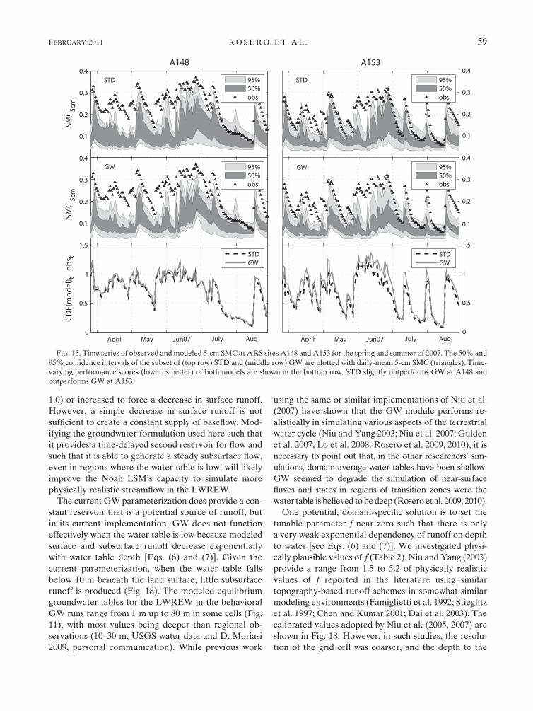
FIG. 15. Time series of observed and modeled 5-cm SMC at ARS sites A148 and A153 for the spring and summer of 2007. The 50% and

95% confidence intervals of the subset of (top row) STD and (middle row) GW are plotted with daily-mean 5-cm SMC (triangles). Time-

varying performance scores (lower is better) of both models are shown in the bottom row. STD slightly outperforms GW at A148 and

outperforms GW at A153.


(parameterized) water table was relatively shallow, which

made the exponential component of the subsurface runoff

significantly greater [see Eq. (7)]. The ideal value of f

likely changes with gridcell size, soil properties, modeled

equilibrium depth to water, and host model (Rosero et al.

2009). By comparing our runs with those of other re-

searchers’ results we clearly see that f must be treated as a

scale-dependent tunable parameter, not a physical quantity.

We also note that a potential explanation for the deeper-

than-observed modeled water table is an overly robust

parameterization of soil matric potential, which sucks

water from the overly deep groundwater reservoir and

contributes to significantly overestimated ET (Fig. 17).

Other potential explanations for the poor quality of

simulated streamflow are that the soil hydrology repre-

sentation of Noah is insufficiently complex and/or not

realistic. This potential limitation is consistent with the

poor-quality behavioral simulations of STD runoff,

which appear to result from the model’s low soil-water

residence time. The increasing or constant CV with in-

creasing mean soil moisture implies that the model does

not have the capacity to retain or to buffer soil moisture.

That is, model grid cells with high porosity likely have

larger mean moisture because they occasionally are briefly

saturated; however, all cells, including the cells that are

wetter on average, dry quickly. For cells with higher po-

rosity, this behavior increases the CV of soil moisture

content. Such quick-to-wet, quick-to-dry behavior may be

ameliorated by increasing the number of layers in the

modeled soil column. However, such a change may be in-

sufficient to fundamentally alter the statistics of the mod-

eled soil moisture.

It is worth noting that Famiglietti et al. (2008), working

in the same region, observed an overall increase in

skewness with the scale of soil moisture measurements,

which implies that positive skewness of the soil moisture

distribution under dry surface conditions may be more

pronounced at the larger end of a range of scales. This

observation may help explain why our 4-km soil-moisture

simulations have skewness values that are much larger

than those of observations.

The runoff parameterizations within GW are related to

topography but do not actually depend on the statistics of

topography. In the development of the physically based

parameterization of GW it was assumed that identification

of parameters that, by derivation, are related to topogra-

phy (fsatmx and rsbmax) has the potential to capture the

heterogeneity of the land features and improve both

FIG. 16. As in Fig. 15, but for 25-cm SMC. GW outperforms STD at site A148; the models are approximately equally well suited to

simulate site A153.


simulated runoff and simulated soil moisture. Our sensi-

tivity analysis showed that adjusting parameter rsbmx

within GW to better reflect within-watershed variations of

topography has little to no effect in improving both the

statistics of soil moisture and the realism of the simulation

of runoff. In the derivation in of the simplified model,

Niu and Yang (2003) state ‘‘it is attractive to develop a

topography-related runoff parameterization which does

not require the topographic index data set. In the simplest

case, the topographic characteristics may be parameter-

ized as constants for all land points, and the saturated

fraction and subsurface runoffs are only determined by the

soil moisture represented by the water table depth.’’ It is

evident that the dependency of the gridcell topography is

largely lost when using the simplification embedded within

the maximum rate of subsurface runoff (rsbmx). Similarly,

the conceptual maximum saturated fraction (fsatmx) be-

comes a tunable parameter. Hence, GW’s simplifications

for surface and subsurface runoff used here are discon-

nected from the actual physics of topographic influence on

groundwater discharge. It is therefore not surprising that,

without extensive calibration, they do not yield significant

improvement in the physical realism of model simulations.

In the LWREW, a combination approach may be war-

ranted. GW is a modified saturation-excess runoff scheme,

which is valid in humid regions, zones with large infil-

tration capacity, and well-distributed precipitation. STD

uses an infiltration-excess scheme, which is better suited to

dry regions with sparse, localized rain or in humid areas

where soils are impermeable.

To accurately predict streamflow or other hydrologic

fluxes and states, choosing the appropriate model struc-

ture (and model parameters) is a crucial step in hydrologic

modeling. The same can be said about understanding the

dominant physical controls on the response of a watershed

(Clark et al. 2008). In land surface modeling, often a

bottom-up approach is followed (as is done here). LSM

are complex structures that generally require detailed in-

formation of the physical characteristics of the modeled

watersheds and are often potentially overparameterized.

As pointed out by Jakeman and Hornberger (1993),

model overparameterization is particularly acute when

simulating streamflow. Instead, and in the context of hy-

pothesis testing, a top-down approach to model de-

velopment is advisable (e.g., Farmer et al. 2003; Schultz

and Beven 2003; Sivapalan et al. 2003; Bai et al. 2009). The

aim should be to identify a model structure with the mi-

nimum level of complexity that is capable of reproducing

the observed watershed response for the ‘‘right reasons’’

(Kirchner 2006). The gap between the simplified hydro-

logical model components implemented in atmospheric

models and the state-of-the-art integrated hydrological

models (Overgaard et al. 2006) can only be bridged with

approaches that systematically increase the complexity of

FIG. 17. Time series of simulated and observed ET at FLUXNET site Little Washita (Fig. 1a) for 1998. Black dots

are hourly ET observations. Daily-mean observed values (black line) are significantly less variable and have a lower

mean value than do the simulated daily-mean values (a) STD (b) GW. Both the 50% and 90% intervals of the

behavioral subset of GW realizations overestimate ET.


the subsurface hydrologic parameterization in a frame-

work that acknowledges explicitly the inherent un-

certainty of the problem (Clark et al. 2008).

Acknowledgments. The first author was supported by

the Graduate Fellowship of the Hydrology Training

Program of the OHD/NWS. The project was also funded

by the NOAA Grant NA07OAR4310216, the NOAA-

CPPA Proposal GC08-521, NSF, and the Jackson School

of Geosciences. Bailing Li, at NASA/GSFC, provided us

with 1 km-LIS land-cover, monthly vegetation fraction

and albedo climatology data. The NEXRAD stage IV

was prepared by Seungbum Hong at UT Austin. We

acknowledge the USGS, ARS micronet and AmeriFlux

for the validation datasets. We thank D. J. Gochis at

NCAR and K. Mitchell at NCEP for their insight. We

benefited from the computational resources at the Texas

Advanced Computing Center (TACC).

REFERENCES

Allen, P. B., and J. W. Naney, 1991: Hydrology of the Little

Washita River Watershed, Oklahoma: Data and analyses.

U.S. Department of Agriculture, Agricultural Research Ser-

vice, ARS-90, 74 pp.

Bai, Y., T. Wagener, and P. Reed, 2009: A top-down framework for

watershed model evaluation and selection under uncertainty.

Environ. Model. Software, 24, 901–916, doi:10.1016/j.envsoft.

2008.12.012.

Bastidas, L. A., T. S. Hogue, S. Sorooshian, H. V. Gupta, and

W. J. Shuttleworth, 2006: Parameter sensitivity analysis for

different complexity land surface models using multicriteria

methods. J. Geophys. Res., 111, D20101, doi:10.1029/

2005JD006377.

Bates, B. C., Z. W. Kundzewicz, S. Wu, and J. P. Palutikof, 2008:

Climate change and water. Intergovernmental Panel on Cli-

mate Change Tech. Paper, 210 pp.

Beven, K. J., 1989: Changing ideas of hydrology: The case of

physically based models. J. Hydrol., 105, 157–172.

——, 2001: How far can we go in distributed hydrological model-

ling? Hydrol. Earth Syst. Sci., 5, 1–12.

——, 2002: Towards an alternative blueprint for a physically based

digitally simulated hydrologic response modelling system.

Hydrol. Processes, 16, 189–206.

——, and A. Binley, 1992: The future of distributed models: Model

calibration and uncertainty prediction. Hydrol. Processes, 6,

279–298.

Boone, A., and Coauthors, 2004: The Rhone-Aggregation Land Sur-

face Scheme intercomparison project: An overview. J. Climate,

17, 187–208.

Box, G. E. P., and D. R. Cox, 1964: An analysis of transformations.

J. Roy. Stat. Soc., 26, 211–252.

Chen, F., and J. Dudhia, 2001: Coupling an advanced land surface–

hydrology model with the Penn State–NCAR MM5 modeling

system. Part I: Model implementation and sensitivity. Mon.

Wea. Rev., 129, 569–586.

——, and Coauthors, 1996: Modeling of land surface evaporation

by four schemes and comparison with FIFE observations.

J. Geophys. Res., 101 (D3), 7251–7268.

Chen, J., and P. Kumar, 2001: Topographic influence on the sea-

sonal and inter-annual variation of water and energy balance

of basins in North America. J. Climate, 14, 1989–2014.

Chen, T. H., and Coauthors, 1997: Cabauw experimental results

from the Project for Intercomparison of Land-Surface Pa-

rameterization Schemes. J. Climate, 10, 1194–1215.

Clapp, R. B., and G. M. Hornberger, 1978: Empirical equations for

some soil hydraulic properties. Water Resour. Res., 14, 601–604.

Clark, M. P., A. G. Slater, D. E. Rupp, R. A. Woods, J. A. Vrugt,

H. V. Gupta, T. Wagener, and L. E. Hay, 2008: Framework for

Understanding Structural Errors (FUSE): A modular frame-

work to diagnose differences between hydrological models.

Water Resour. Res., 44, W00B02, doi:10.1029/2007WR006735.

FIG. 18. Sensitivity of GW’s (a) surface and (b) subsurface runoff to depth to water table (zwt) and e-folding depth

f (exponential decay of saturated hydraulic conductivity). Dashed lines are values of calibrated parameters used by

Niu et al. (2005; 2007).


Cosgrove, B. A., and Coauthors, 2003: Real-time and retrospective

forcing in the North American Land Data Assimilation System

(NLDAS) project. J. Geophys. Res., 108, 8842, doi:10.1029/

2002JD003118.

Dai, Y., and Coauthors, 2003: The Common Land Model. Bull.

Amer. Meteor. Soc., 84, 1013–1023.

Dirmeyer, P. A., 2006: The hydrologic feedback pathway for land–

climate coupling. J. Hydrometeor., 7, 857–867.

Ducharne, A., R. D. Koster, M. J. Suarez, M. Stieglitz, and

P. Kumar, 2000: A catchment-based approach to modeling

land surface processes in a general circulation model 2. Pa-

rameter estimation and model demonstration. J. Geophys.

Res., 105 (D20), 24 823–24 838.

Ek, M. B., K. E. Mitchell, Y. Lin, E. Rogers, P. Grunmann,

V. Koren, G. Gayno, and J. D. Tarpley, 2003: Implementa-

tion of Noah land surface model advances in the National

Centers for Environmental Prediction operational meso-

scale Eta model. J. Geophys. Res., 108, 8851, doi:10.1029/

2002JD003296.

Famiglietti, J. S., E. F. Wood, M. Sivapalan, and D. J. Thongs, 1992:

A catchment scale water balance model for FIFE. J. Geophys.

Res., 97, 18 997–19 007.

——, D. Ryu, A. A. Berg, M. Rodell, and T. J. Jackson, 2008: Field

observations of soil moisture variability across scales. Water

Resour. Res., 44, W01423, doi:10.1029/2006WR005804.

Fan, Y., G. Miguez-Macho, C. P. Weaver, R. Walko, and A. Robock,

2007: Incorporating water table dynamics in climate modeling:

1. Water table observations and the equilibrium water table.

J. Geophys. Res., 112, D10125, doi:10.1029/2006JD008111.

Farmer, D., M. Sivapalan, and C. Jothityangkoon, 2003: Climate,

soil, and vegetation controls upon the variability of water

balance in temperate and semiarid landscapes: Downward

approach to water balance analysis. Water Resour. Res., 39,

1035, doi:10.1029/2001WR000328.

Gulden, L. E., E. Rosero, Z.-L. Yang, M. Rodell, C. S. Jackson,

G.-Y. Niu, P. J.-F. Yeh, and J. Famiglietti, 2007: Improving

land-surface model hydrology: Is an explicit aquifer model

better than a deeper soil profile? Geophys. Res. Lett., 34,

L09402, doi:10.1029/2007GL029804.

——, ——, ——, T. Wagener, and G.-Y. Niu, 2008: Model per-

formance, model robustness, and model fitness scores: A new

method for identifying good land-surface models. Geophys.

Res. Lett., 35, L11404, doi:10.1029/2008GL033721.

Gutowski, W. J., Jr., C. J. Vorosmarty, M. Person, Z. Otles,

B. Fekete, and J. York, 2002: A Coupled Land-Atmosphere

Simulation Program (CLASP): Calibration and validation.

J. Geophys. Res., 107, 4283, doi:10.1029/2001JD000392.

Hansen, M. C., R. S. DeFries, J. R. G. Townshend, and R. Sohlberg,

2000: Global land cover classification at 1 km spatial resolution

using a classification tree approach. Int. J. Remote Sens., 21 (6-7),

1389–1414.

Hogue, T. S., L. A. Bastidas, H. V. Gupta, and S. Sorooshian, 2006:

Evaluating model performance and parameter behavior for

varying levels of land surface model complexity. Water Re-

sour. Res., 42, W08430, doi:10.1029/2005WR004440.

Hornberger, G. M., and R. C. Spear, 1981: An approach to the

preliminary analysis of environmental systems. J. Environ.

Manage., 12, 7–18.

Jakeman, A. J., and G. M. Hornberger, 1993: How much com-

plexity is warranted in a rainfall-runoff model? Water Resour.

Res., 29, 2637–2649.

Kirchner, J. W., 2006: Getting the right answers for the right rea-

sons: Linking measurements, analyses, and models to advance

the science of hydrology. Water Resour. Res., 42, W03S04,

doi:10.1029/2005WR004362.

Kollet, S. J., and R. M. Maxwell, 2008: Capturing the influence of

groundwater dynamics on land surface processes using an in-

tegrated, distributed watershed model. Water Resour. Res., 44,

W02402, doi:10.1029/2007WR006004.

Konikow, L. F., and J. D. Bredehoeft, 1992: Groundwater models

cannot be validated. Adv. Water Resour., 15, 13–24.

Koster, R. D., and P. C. D. Milly, 1997: The interplay between

transpiration and runoff formulations in land surface schemes

used with atmospheric models. J. Climate, 10, 1578–1591.

——, M. J. Suarez, A. Ducharne, M. Stieglitz, and P. Kumar, 2000:

A catchment-based approach to modeling land surface pro-

cesses in a general circulation model 1. Model structure.

J. Geophys. Res., 105 (D20), 24 809–24 822.

Li, H., A. Robock, and M. Wild, 2007: Evaluation of In-

tergovernmental Panel on Climate Change Fourth Assess-

ment soil moisture simulations for the second half of the

twentieth century. J. Geophys. Res., 112, D06106, doi:10.1029/

2006JD007455.

Liang, X., E. F. Wood, and D. P. Lettenmaier, 1996: Surface soil

moisture parameterization of the VIC-2L model: Evaluation

and modification. Global Planet. Change, 13, 195–206.

——, and Coauthors, 1998: The Project for Intercomparison of

Land-surface Parameterization Schemes (PILPS) phase 2(c)

Red-Arkansas River basin experiment: 2. Spatial and tem-

poral analysis of energy fluxes. Global Planet. Change, 19,

137–159.

——, Z. Xie, and M. Huang, 2003: A new parameterization for

surface and groundwater interactions and its impact on

water budgets with the variable infiltration capacity (VIC)

land surface model. J. Geophys. Res., 108, 8613, doi:10.1029/

2002JD003090.

Lo, M. H., P. J. F. Yeh, and J. S. Famiglietti, 2008: Constraining

water table depth simulations in a land surface model using

estimated baseflow. Adv. Water Resour., 31, 1552–1564.

Lohmann, D., and Coauthors, 1998: The Project for Intercomparison

of Land-surface Parameterization Schemes (PILPS) phase

2(c) Red-Arkansas River basin experiment: 3. Spatial and

temporal analysis of water fluxes. Global Planet. Change, 19,

161–179.

Maxwell, R. M., and N. L. Miller, 2005: Development of a cou-

pled land surface and groundwater model. J. Hydrometeor.,

6, 233–247.

McKay, M., R. Beckman, and W. Conover, 1979: A comparison of

three methods for selecting values of input variables in the

analysis of output from a computer code. Technometrics, 21,

239–245.

Meyers, T. P., 2001: A comparison of summertime water and CO2

fluxes over rangeland for well watered and drought conditions.

Agric. For. Meteor., 106, 205–214.

Mitchell, K. E., and Coauthors, 2004: The multi-institution North

American Land Data Assimilation System (NLDAS): Utiliz-

ing multiple GCIP products and partners in a continental

distributed hydrological modeling system. J. Geophys. Res.,

109, D07S90, doi:10.1029/2003JD003823.

Nasonova, O. N., Y. M. Gusev, and Y. E. Kovalev, 2009: In-

vestigating the ability of a land surface model to simulate

streamflow with the accuracy of hydrological models: A case

study using MOPEX materials. J. Hydrometeor., 10, 1128–1150.

Nijseen, B., and L. A. Bastidas, 2005: Land–atmosphere models for

water and energy cycle studies. Encyclopedia of Hydrological

Sciences, M. G. Anderson, Ed., Vol. 5, John Wiley, 3089–3102.


Niu, G.-Y., and Z.-L. Yang, 2003: The versatile integrator of surface

and atmosphere processes (VISA). Part II: Evaluation of three

topography-based runoff schemes. Global Planet. Change, 38,

191–208.

——, ——, R. E. Dickinson, and L. E. Gulden, 2005: A simple

TOPMODEL-based runoff parameterization (SIMTOP) for

use in GCMs. J. Geophys. Res., 110, D21106, doi:10.1029/

2005JD006111.

——, ——, ——, ——, and H. Su, 2007: Development of a simple

groundwater model for use in climate models and evaluation

with Gravity Recovery and Climate Experiment data. J. Geo-

phys. Res., 112, D07103, doi:10.1029/2006JD007522.

Oki, T., T. Nishimura, and P. Dirmeyer, 1999: Assessment of land

surface models by runoff in major river basins of the globe

using Total Runoff Integrating Pathways (TRIP). J. Meteor.

Soc. Japan, 77, 235–255.

Overgaard, J., D. Rosbjerg, and M. B. Butts, 2006: Land-surface

modelling in hydrological perspective—A review. Biogeosciences,

3, 229–241.

Pitman, A. J., 2003: Review: The evolution of, and revolution in,

land surface schemes designed for climate models. Int. J. Cli-

matol., 23, 479–510, doi:10.1002/joc.893.

——, and Coauthors, 1999: Key results and implications from

Phase 1(c) of the Project for Intercomparison of Land-surface

Parameterization Schemes. Climate Dyn., 15, 673–684.

Ratto, M., P. C. Young, R. Romanowicz, F. Pappenberger,

A. Saltelli, and A. Pagano, 2007: Uncertainty, sensitivity

analysis and the role of data based mechanistic modeling in

hydrology. Hydrol. Earth Syst. Sci., 11, 1249–1266.

Refsgaard, J. C., 1997: Parameterization, calibration and validation

of distributed hydrological models. J. Hydrol., 198, 69–97.

——, and H. J. Henriksen, 2004: Modelling guidelines terminology

and guiding principles. Adv. Water Resour., 27, 71–82.

Reichle, R. H., and R. D. Koster, 2005: Global assimilation of

satellite surface soil moisture retrievals into the NASA

Catchment land surface model. Geophys. Res. Lett., 32,

L02404, doi:10.1029/2004GL021700.

Rosero, E., Z.-L. Yang, L. E. Gulden, G.-Y. Niu, and D. J. Gochis,

2009: Evaluating enhanced hydrological representations in

Noah LSM over transition zones: Implications for model de-

velopment. J. Hydrometeor., 10, 600–622.

——, ——, T. Wagener, L. E. Gulden, S. Yatheendradas, and

G.-Y. Niu, 2010: Quantifying parameter sensitivity, interaction

and transferability in hydrologically enhanced versions of

Noah-LSM over transition zones. J. Geophys. Res., 115,D03106, doi:10.1029/2009JD012035.

Saltelli, A., 2002: Making best use of model evaluations to compute

sensitivity indices. Comput. Phys. Commun., 145, 280–297.

——, A. Tarantola, F. Campolongo, and M. Ratto, 2004: Sensitivity

Analysis in Practice: A Guide to Assessing Scientific Models.

John Wiley and Sons, 232 pp.

Schaake, J. C., V. I. Koren, Q.-Y. Duan, K. Mitchell, and F. Chen,

1996: Simple water balance model for estimating runoff at

different spatial and temporal scales. J. Geophys. Res., 101

(D3), 7461–7475.

Schultz, K., and K. Beven, 2003: Data-supported robust parame-

terizations in land surface–atmosphere flux predictions: To-

ward a top-down approach. Hydrol. Processes, 17, 2259–2277.

Sivapalan, M., K. Beven, and E. F. Wood, 1987: On hydrologic

similarity: 2. A scaled model of storm runoff production. Water

Resour. Res., 23, 2266–2278.

——, G. Bloschl, L. Zhang, and R. Vertessy, 2003: Downward

approach to hydrological prediction. Hydrol. Processes, 17,

2101–2111, doi:10.1002/hyp.1425.

Smakhtin, U., 2001: Low flow hydrology: A review. J. Hydrol., 240,147–186.

Sobol’, I. M., 1993: Sensitivity analysis for nonlinear mathematical

models. Math. Models Comput. Exp., 1, 407–414.

——, 2001: Global sensitivity indices for nonlinear mathematical

models and their Monte Carlo estimates. Math. Comput. Si-

mul., 55, 271–280, doi:10.1016/S0378-4754(00)00270-6.

Soil Survey Staff, cited 2009: U.S. General Soil Map (STATSGO2)

for Oklahoma. Natural Resources Conservation Service,

United States Department of Agriculture. [Available online at

http://soildatamart.nrcs.usda.gov.]

Sorooshian, S., and J. A. Dracup, 1980: Stochastic parameter esti-

mation procedures for hydrologic rainfall-runoff models:

Correlated and heteroscedastic error cases. Water Resour.

Res., 16, 430–442.

Stieglitz, M., D. Rind, J. Famiglietti, and C. Rosenzweig, 1997: An

efficient approach to modeling the topographic control of

surface hydrology for regional and global modeling. J. Cli-

mate, 10, 118–137.

Stockli, R., P. L. Vidale, A. Boone, and C. Schar, 2007: Impact of

scale and aggregation on the terrestrial water exchange: In-

tegrating land surface models and Rhone catchment obser-

vations. J. Hydrometeor., 8, 1002–1015.

——, and Coauthors, 2008: Use of FLUXNET in the Community

Land Model development. J. Geophys. Res., 113, G01025,

doi:10.1029/2007JG000562.

van Werkhoven, K., T. Wagener, P. Reed, and Y. Tang, 2008:

Characterization of watershed model behavior across a hy-

droclimatic gradient. Water Resour. Res., 44, W01429,

doi:10.1029/2007WR006271.

Viterbo, P., 2002: A review of parametrization schemes for land sur-

face processes. Meteorological Training Course Lecture Series,

ECMWF, Shinfield Park, Reading, United Kingdom, 1–49.

Vogel, R. M., and N. M. Fennessey, 1994: Flow duration curves. I.

A new interpretation and confidence intervals. J. Water Re-

sour. Plann. Manage., 120, 485–504.

Wagener, T., M. Sivapalan, P. Troch, and R. Woods, 2007:

Catchment classification and hydrologic similarity. Geogr.

Compass, 1, 901–931, doi:10.1111/j.1749-8198.2007.00039.x.

Wetzel, P., and Coauthors, 1996: Modeling vadose zone liquid

water fluxes: Infiltration, runoff, drainage, interflow. Global

Planet. Change, 13, 57–71.

Wood, E. F., D. P. Lettenmaier, and V. G. Zartarian, 1992: A land-

surface hydrology parameterization with subgrid variability

for general circulation models. J. Geophys. Res., 97 (D3),

2717–2728.

——, and Coauthors, 1998: The Project for Intercomparison of

Land-surface Parameterization Schemes (PILPS) phase 2(c)

Red-Arkansas River basin experiment: 1. Experiment de-

scription and summary intercomparisons. Global Planet.

Change, 19, 115–135.

Yeh, P. J.-F., and E. A. B. Eltahir, 2005: Representation of water

table dynamics in a land-surface scheme. Part I: Model de-

velopment. J. Climate, 18, 1861–1880.

Yilmaz, K. K., H. V. Gupta, and T. Wagener, 2008: A process-

based diagnostic approach to model evaluation: Application

to the NWS distributed hydrologic model. Water Resour. Res.,

44, W09417, doi:10.1029/2007WR006716.


Copyright of Journal of Hydrometeorology is the property of American Meteorological Society and its content

may not be copied or emailed to multiple sites or posted to a listserv without the copyright holder's express

written permission. However, users may print, download, or email articles for individual use.

ensemble evaluation of hydrologically enhanced noah-lsm

Documents