Clarke et al. BMC Bioinformatics (2016) 17:380 DOI 10.1186/s12859-016-1245-9

SOFTWARE Open Access

EnsCat: clustering of categorical data viaensemblingBertrand S. Clarke1, Saeid Amiri2 and Jennifer L. Clarke1,3*

Abstract

Background: Clustering is a widely used collection of unsupervised learning techniques for identifying naturalclasses within a data set. It is often used in bioinformatics to infer population substructure. Genomic data are oftencategorical and high dimensional, e.g., long sequences of nucleotides. This makes inference challenging: The distancemetric is often not well-defined on categorical data; running time for computations using high dimensional data canbe considerable; and the Curse of Dimensionality often impedes the interpretation of the results. Up to the present,however, the literature and software addressing clustering for categorical data has not yet led to a standard approach.

Results: We present software for an ensemble method that performs well in comparison with other methodsregardless of the dimensionality of the data. In an ensemble method a variety of instantiations of a statistical objectare found and then combined into a consensus value. It has been known for decades that ensembling generallyoutperforms the components that comprise it in many settings. Here, we apply this ensembling principle to clustering.We begin by generating many hierarchical clusterings with different clustering sizes. When the dimension of the datais high, we also randomly select subspaces also of variable size, to generate clusterings. Then, we combine theseclusterings into a single membership matrix and use this to obtain a new, ensembled dissimilarity matrix usingHamming distance.

Conclusions: Ensemble clustering, as implemented in R and called EnsCat, gives more clearly separated clusters thanother clustering techniques for categorical data. The latest version with manual and examples is available athttps://github.com/jlp2duke/EnsCat.

Keywords: Categorical data, Clustering, Ensembling methods, High dimensional data

BackgroundThe idea of clustering is to group unlabeled data intosubsets so that both the within-group homogeneity andthe between-group heterogeneity are high. The hope isthat the groups will reflect the underlying structure ofthe data generator. Although clustering continuous datacan be done in a wide variety of conceptually distinctways there are generally far fewer techniques for cat-egorical data. Probably the most familiar methods areK-modes [1], model-based clustering (MBC) [2], and vari-ous forms of hierarchical clustering. K-modes is K-meansadapted to categorical data by replacing cluster means

*Correspondence: jclarke3@unl.edu1Department of Statistics, University of Nebraska-Lincoln, Lincoln, NE, USA3Department of Food Science and Technology, University of Nebraska-Lincoln,Lincoln, NE, USAFull list of author information is available at the end of the article

with cluster modes. MBC postulates a collection of mod-els and assumes the clusters are representative of a mix-ture of those models. The weights on the models and theparameters in the model are typically estimated from thedata. Hierarchical clustering is based on choosing a senseof distance between points and then merging data pointsor partitioning the data set, agglomerative or divisive,respectively. The merge or partition rules in a hierarchicalmethod must also be chosen. So, hierarchical clusteringis actually a large collection of techniques. Other morerecent approaches include ROCK [3], which is based ona notion of graph-theoretic connectivity between points,and CLICK [4], which is based on finding fully connectedsubgraphs in low dimensional subspaces.Ensembling is a general approach to finding a consensus

value of some quantity that typically gives better perfor-mance than any one of the components used to form it.

© 2016 The Author(s). Open Access This article is distributed under the terms of the Creative Commons Attribution 4.0International License (http://creativecommons.org/licenses/by/4.0/), which permits unrestricted use, distribution, andreproduction in any medium, provided you give appropriate credit to the original author(s) and the source, provide a link to theCreative Commons license, and indicate if changes were made. The Creative Commons Public Domain Dedication waiver(http://creativecommons.org/publicdomain/zero/1.0/) applies to the data made available in this article, unless otherwise stated.

Clarke et al. BMC Bioinformatics (2016) 17:380 Page 2 of 13

In the clustering context, this means that we should beable to take a collection of clusterings and somehowmergethem so they will yield a consensus clustering that is betterthan any of the individual clusterings, possibly by separat-ing clusters more cleanly or having some other desirableproperty. Thus, in principle, ensembling can be used onany collection of clusterings, however obtained.There are many techniques by which the ensembling

of clusters can be done and many techniques by whichclusters to be ensembled can be generated. For instance,in the case of continuous data, four alternative methodsfor ensembling clusters are studied in [5]. They can alsoin some cases be applied to categorical data. The best ofthe four seems to be a form of model based clusteringthat rests on discretizing a data set, imputing classes tothe various clusters from a collection of clusterings, andmodeling the imputed classes by a mixture of discrete dis-tributions. These methods were exemplified on five lowdimensional data sets (maximum dimension 14) and eventhough the model based approach was overall best, theother methods were often a close second and in somecases better.More recently, [6] developed a consensus clustering

based on resampling. Any clustering technique can berepeatedly applied. Essentially, the proportion of timesdata points are put in the same cluster defines a collec-tion of pairwise consensus values which are used to formK consensus clusters for given K. The ensembling methodused in [6] does not seem to have been compared to themethods studied in [5]. In addition, most recently, the R-package CLUE (most recent instantiation 2016) ensemblesclusters using a different and more general concept of dis-tance than in [5] or [6] although neither of those may beregarded as special cases of CLUE.By contrast, to ensemble clusterings, we ensemble dis-

similarity matrices rather than cluster indices and weassume the data are categorical. Thus, our method isagain different from those that have been presented. Ourmethod starts by forming an incidence matrix I summa-rizing all of them. The number of columns in I is the num-ber of clusterings, sayB; each column has n entries, one foreach data point. The (i, j) entry of I is the index of the clus-ter in the j-th clustering to which xi belongs. The Ham-ming distances between pairs of rows in the incidencematrix effectively sums over clusterings – combining theireffects – and gives a distance between each pair of datapoints. These distances are the entries in the ensembleddissimilarity matrix that we use in our approach. Thisform of ensembling is described in detail in [7]. Note thatthe individual clusterings that go in to forming the ensem-bled dissimilarity matrix are unrestricted; they may evenbe of different sizes.We have used Hamming distance with equal weights

since it is natural for discrete data when the principle

of insufficient reason applies1 – it corresponds to clas-sification loss which assumes the values are categoricalrather than discrete ordinal and does not weight any onecategorical variable more or less than any other. Implic-itly Hamming distance also assumes that all distancesbetween values of the same random variable are the same.Hence it is a good default when no extra information isavailable. Indeed, it is well known that different senses ofdistance correspond to different clustering criteria. Deter-mining which sense of distance is appropriate for a givensetting is a difficult and general problem. It is beyondthe scope of this paper which is merely to present thesoftware.Given this, the question is which base clusterings to

ensemble. Recall that with categorical data the measure-ments on a subject form a vector of discrete unorderedvalues. Here, we will assume there is a uniform bound onthe number of values each variable can assume. Data sat-isfying this condition is common in genetics because thenucleotide at a location is one of four values. We haveensembled a variety of clusterings generated by variousmethods. For instance, we have ensembled K-modes clus-terings, model based clusterings (also called latent classclustering in some settings), and hierarchical clusteringsusing Hamming distance and several different linkages.2As seen in [7], the best clustering results seem to emergeby i) generating hierarchical clusterings using Hammingdistance and average linkage, ii) combining them intothe ensembled dissimilarity matrix (again using Hammingdistance), and iii) using hierarchical clustering with, say,average linkage as defined by the ensembled dissimilaritymatrix. Variants on this procedure also seem to work well,e.g., complete linkage gives similar performance to aver-age linkage and ensembling reduces the chaining problem(see [8]) associated with single linkage. Metrics other thanHamming distance may give better or worse results, butwe have not investigated this because Hamming distanceis such an intuitively reasonable way to assess distancesbetween categorical vectors.This procedure outperforms K-modes because, when

the data are categorical, the mean is not well-defined.So, using the mode of a cluster as its ‘center’ often doesnot represent the location of a cluster well. Moreover, K-modes can depend strongly on the initial values. Usingsummary statistics that are continuous does not resolvethis problem either; see [9] for an example.Our procedure outperforms MBC because MBC relies

on having a model that is both accurate and parsimo-nious – a difficult input to identify for complex data.Indeed, if we know so much about the data that we canidentify good models, it must be asked why we need clus-tering at all – except possibly to estimate parameters suchas model weights. As a separate issue MBC is compu-tationally much more demanding than our method. We

Clarke et al. BMC Bioinformatics (2016) 17:380 Page 3 of 13

comment that in some cases, the ensemble clustering canbe worse than simply using a fixed clusteringmethod. Thisis often the case for K-modes and MBC. While some-what counterintuitive, this is a well recognized propertyof other ensemble methods, such as bagging, becauseensemble methods typically only give improvement onaverage.Overall, in [7] our method was compared to 13 other

methods (including model based clustering) over 11 realcategorical data sets and numerous systematic simulationstudies of categorical data in low and high dimensionalsettings. The theory established suggests that ensembleclustering is more accurate than non-ensembled cluster-ings because ensembling reduces the variability of clus-tering. Our finding that the method implemented here is‘best’ is only in an average sense for the range of prob-lems we examined among the range of techniques wetested. In all these cases, our ensembled method was thebest, or nearly so, and its closest competitors on averagewere non-emsembled hierarchical methods that also usedHamming distance as a dissimilarity. Thus, in the presentpaper, we only compare our ensemble method with itsnon-ensembled counterpart.At root, our method generates an ensembled dissimilar-

ity matrix that seems to represent the distances betweenpoints better than the dissimilarity matrices used to formit. The result, typically, is that we get dendrograms thatseparate clusters more clearly than other methods. Thus,simply looking at the dendrogram is a good way to choosethe appropriate number of clusters.To fix notation, we assume n independent and identi-

cal (IID) outcomes xi, i = 1, . . . , n, of a random variableX. The xi’s are assumed J-dimensional and written as(xi1, . . . , xiJ ) where each xij is categorical and assumes nomore than, say, M values. We consider three cases for thevalue J : Low dimension, i.e., n � J , high dimension, i.e.,J � n, and high dimension but unequal, i.e., different xi’scan have different J ’s and all the J ’s are much larger thann. We implemented our procedure for these three cases inan R package, entitled EnsCat. As will be seen, the basictechnique is for low dimensional data but scales up to highdimensional data by using random selection of subspacesand increasing the size of the ensemble. This is extendedto data vectors that do not have a common length by usingmultiple alignment. We present these cases below.

ImplementationWe implemented our methods in the R statistical lan-guage that is free and open source [10]. So, our packagedoes not require any other software directly. Since R isalready widely used by researchers, we limit our presen-tation below to the functions we have defined in Enscat.The one exception to this is that if one wants to use oursoftware on unequal length data e.g., genome sequences,

the data points must be aligned and our software is com-patible with any aligner. Several aligners are available in R,however, they have long running times for genome lengthdata. As noted below, we convert categorical data valuessuch as {A,T ,C,G} to numerical values such as 1,2,3,4because R runs faster on numerical values than on char-acter values, and numerical values require less storagecapacity.When J is large, our methodology uses a random sub-

space approach to reduce the dimension of the vectorsbeing clustered. We do this by bootstrapping. Given theset {1, . . . , J} we choose a sample of size J with replace-ment, i.e., we take J IID draws from {1, . . . , J}. Then weeliminate multiplicity to get a set of size J∗ ≤ J of dis-tinct elements. This procedure can be repeated on the setwith J∗ elements, if desired, to get a smaller set of distinctdimensions. Since the dimensions of the subspaces arerandom, they will, in general, be different. This allows ourprocedure to encapsulate a large number of relationshipsamong the entires in the xi’s. As a generality, ensemblemethods are robust by construction because they rep-resent a consensus of the components being ensembled.This is formally true for random forests in classificationcontexts, [11], and partially explains why ensemble meth-ods are not always optimal. Sometimes a single compo-nent routinely outperforms ensembles of them; this seemsto be the case with K-modes and MBC.

Results and discussionLow dimensional categorical dataThe package Enscat includes functions for implement-ing K-modes, hierarchical clustering methods, and ourensemble clustering method. It can also call routines forMBC. To show how this works, here we use the data setUSFlag as an example. This dataset contains informationabout maritime vessels in the U.S.-Flag Privately-OwnedFleet and can be downloaded from the United StatesDepartment of Transportation site for United StatesMaritime Administration data and statistics [12]. USFlaghas sample size n = 170 and each observation has 10categorical variables containing information about ves-sel operator, vessel size and weight, and vessel type(Containership, Dry Bulk, General Cargo, Ro-Ro, andTanker, denoted as 1 through 5). The data are storedin USFlag$obs and the vessel types are stored inUSFlag$lab. Once the Enscat package has been down-loaded and installed, K-modes clustering can be done in Rby using the commands

library(EnsCat) (1)data(USFlag)kmodes(USFlag$obs, k=5,k2=1:5)

The second argument in the function kmodes,k=5, isthe number of clusters K-modes should output. The third

Clarke et al. BMC Bioinformatics (2016) 17:380 Page 4 of 13

argument is the specification of the initial modes. Here,1:5 means the first five data points should be taken asthe initial modes. As recognized in [1], K-modes is sen-sitive to initial values, possibly leading to instability andinaccuracy.Hierarchical clustering has attracted more attention

than K-modes since it provides a nested sequence of clus-terings that can be represented as a tree or dendrogram.This technique requires a matrix specifying the distancesbetween data points; such a matrix can be calculatedusing Hamming distance. The following commands gen-erate a dendrogram using Hamming distance and averagelinkage.

distham0<-hammingD(USFlag$obs)

distham<-as.dist(distham0)

hcham<-hclust(distham,method="average")

ggdplot(hcham, lab=USFlag$lab, title=

"average linkage hclust of USFlag data")

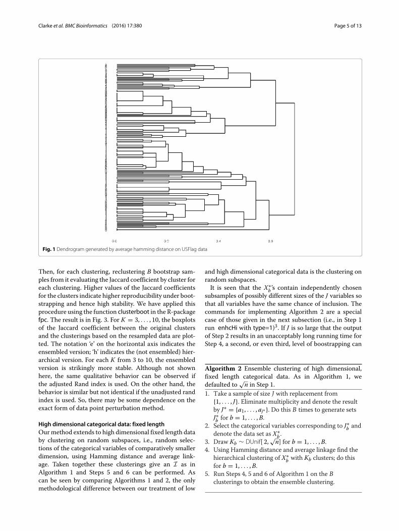
The first command generates the n × nmatrix in whichthe (i, j)-th entry is (1/J)H(xi, xj) ∈[ 0, 1] where H is theHamming distance between its arguments. The secondcommand tells R to regard distham0 as a matrix of dis-tance. Taken together, the third and fourth commandsproduce and plot the dendrogram for hierarchical cluster-ing using distham0 and average linkage. The commandggdplot is a convenience wrapper for the function ggden-drogram in the package ggdendro which automates theplotting of a rotated dendrogram with user specified leaflabels and plot title. The results are shown in Fig. 1.By contrast, our ensembling algorithm is the following.Ensemble clustering of USFlag can be done by the

following.

disten<-Benhc(USFlag$obs,En=200)

en<-hclust(disten,method=’average’)

ggdplot(en, lab=USFlag$lab, ptype=2)

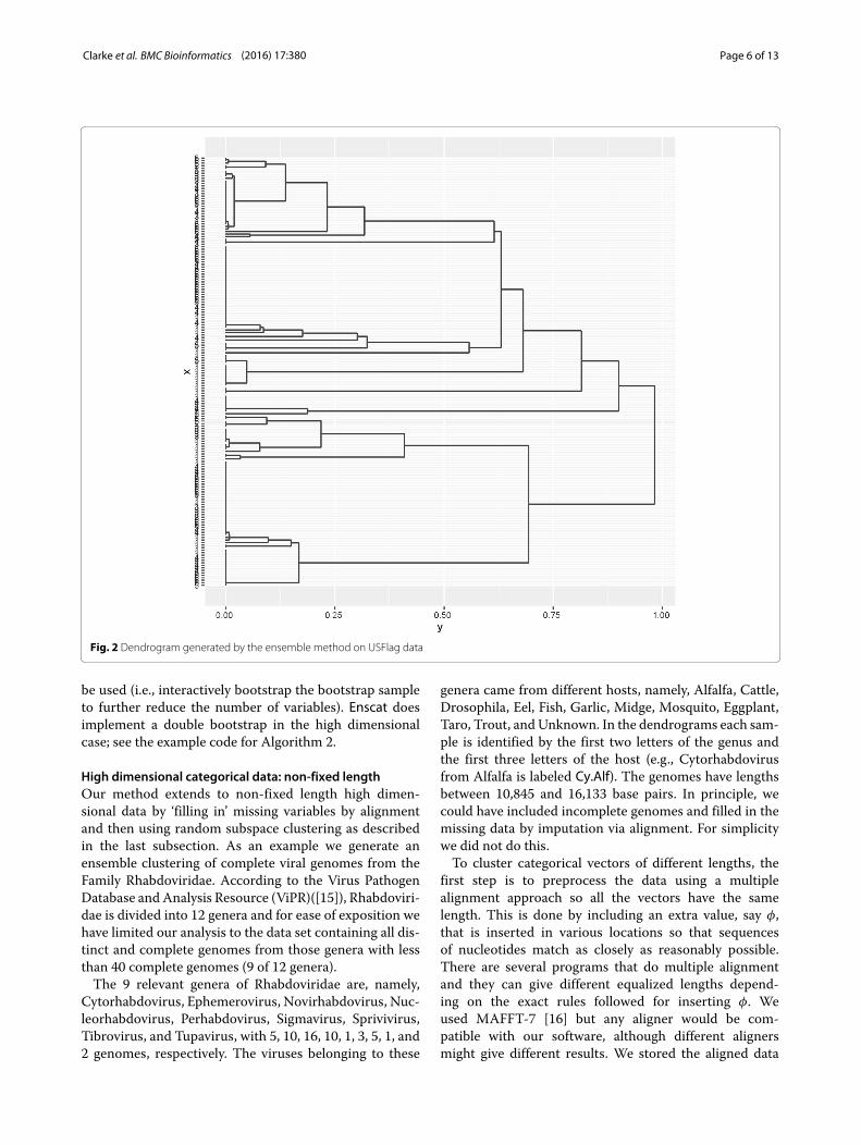
The first command uses Benhc, one of two functionsin Enscat that implement our new method. This gener-ates the ensembled dissimilarity matrix T by combiningB = 200 hierarchical clusterings using Hamming distanceand average linkage, each generated by Steps 1, 2, and 3 inAlgorithm 1. (As a generality, average linkage was foundto perform well in this context, see [7].) The second com-mand runs a hierarchical clustering using T and averagelinkage. hclust is a function in R from the package statsthat can be used to make a dendrogram. The third com-mand generates a plot of the ensembled dendrogram, witha grayscale grid in the background to help gauge the lengthof each lifetime; see Fig. 2. In contrast with Fig. 1, theensembling gives longer ‘lifetimes’, i.e., the vertical linesconnecting to the individual data points. Longer lifetimesmean that the clusters are separated more clearly. Wefound this to be the typical effect of ensembling.

Algorithm 1 Ensemble clustering for low dimensionaldata. We defaulted to

√n in Step 1, but other choices are

possible

1. Draw Kb ∼ DUnif[ 2,√n] for b = 1, . . . ,B.

2. For each b, take a sample (with replacement) Xb fromthe original data.

3. Generate a clustering with Kb clusters for Xb by anyclustering procedure.

4. Form the incidence matrix

I =⎡⎢⎣w12 w12 . . . w1B...

......

...wn1 wn2 . . . wnB

⎤⎥⎦

Each column in I corresponds to one of the Bclusterings and wib is the index of the cluster in theb-th clustering to which xi belongs.

5. Find the ensembled dissimilarity matrix T from Iwhere

T = (dB(xi, xj))i,j=1,...,n,

in which

dB(xi, xj) = 1B

B∑b=1

δ(wib,wjb).

and δ(·, ·) is one minus the indicator function for theequality of its arguments.

6. Use hierarchical clustering on T with any linkagefunction to plot the dendrogram for the ensembleclustering.

Estimating the correct number of clusters, KT , is a dif-ficult problem. Several consistent methods are known forcontinuous data, see [13] for a discussion and comparisonof such techniques. In the categorical data context, sometechniques such as K-modes and MBC require K as aninput and in practice the user chooses the value of K thatgives the most satisfactory results. For hierarchical clus-tering, K need not be pre-assigned; it can be inferred, atleast heuristically, from the dendrogram. When ensem-bling separates the clusters more clearly inferring K maybe easier. In particular, it can be seen from the increasednumber of long lifetimes in the dendrogram of Fig. 2 rela-tive to the number of long lifetimes in the dendrogram ofFig. 1 that the ensembling visibly improves the separabil-ity of the clusters leading to fewer, more distinct clusters.Thus, simply looking at the dendrogram may be a goodway to choose the appropriate number of clusters.This observation is heuristic but is supported by for-

mal stability computations under perturbation indices, forinstance. One established approach is due to [14]. Theidea is to generate a range of clusterings of various sizes.

Clarke et al. BMC Bioinformatics (2016) 17:380 Page 5 of 13

Fig. 1 Dendrogram generated by average hamming distance on USFlag data

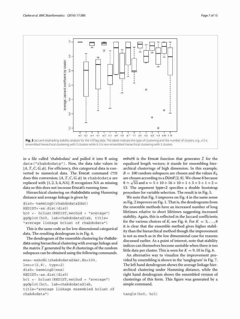
Then, for each clustering, reclustering B bootstrap sam-ples from it evaluating the Jaccard coefficient by cluster foreach clustering. Higher values of the Jaccard coefficientsfor the clusters indicate higher reproducibility under boot-strapping and hence high stability. We have applied thisprocedure using the function clusterboot in the R-packagefpc. The result is in Fig. 3. For K = 3, . . . , 10, the boxplotsof the Jaccard coefficient between the original clustersand the clusterings based on the resampled data are plot-ted. The notation ‘e’ on the horizontal axis indicates theensembled version; ‘h’ indicates the (not ensembled) hier-archical version. For each K from 3 to 10, the ensembledversion is strikingly more stable. Although not shownhere, the same qualitative behavior can be observed ifthe adjusted Rand index is used. On the other hand, thebehavior is similar but not identical if the unadjusted randindex is used. So, there may be some dependence on theexact form of data point perturbation method.

High dimensional categorical data: fixed lengthOurmethod extends to high dimensional fixed length databy clustering on random subspaces, i.e., random selec-tions of the categorical variables of comparatively smallerdimension, using Hamming distance and average link-age. Taken together these clusterings give an I as inAlgorithm 1 and Steps 5 and 6 can be performed. Ascan be seen by comparing Algorithms 1 and 2, the onlymethodological difference between our treatment of low

and high dimensional categorical data is the clustering onrandom subspaces.It is seen that the X∗

b ’s contain independently chosensubsamples of possibly different sizes of the J variables sothat all variables have the same chance of inclusion. Thecommands for implementing Algorithm 2 are a specialcase of those given in the next subsection (i.e., in Step 1run enhcHi with type=1)3. If J is so large that the outputof Step 2 results in an unacceptably long running time forStep 4, a second, or even third, level of boostrapping can

Algorithm 2 Ensemble clustering of high dimensional,fixed length categorical data. As in Algorithm 1, wedefaulted to

√n in Step 1.

1. Take a sample of size J with replacement from{1, . . . , J}. Eliminate multiplicity and denote the resultby J∗ = {a1, . . . , aj∗}. Do this B times to generate setsJ∗b for b = 1, . . . ,B.

2. Select the categorical variables corresponding to J∗b anddenote the data set as X∗

b .3. Draw Kb ∼ DUnif[ 2,

√n] for b = 1, . . . ,B.

4. Using Hamming distance and average linkage find thehierarchical clustering of X∗

b with Kb clusters; do thisfor b = 1, . . . ,B.

5. Run Steps 4, 5 and 6 of Algorithm 1 on the Bclusterings to obtain the ensemble clustering.

Clarke et al. BMC Bioinformatics (2016) 17:380 Page 6 of 13

Fig. 2 Dendrogram generated by the ensemble method on USFlag data

be used (i.e., interactively bootstrap the bootstrap sampleto further reduce the number of variables). Enscat doesimplement a double bootstrap in the high dimensionalcase; see the example code for Algorithm 2.

High dimensional categorical data: non-fixed lengthOur method extends to non-fixed length high dimen-sional data by ‘filling in’ missing variables by alignmentand then using random subspace clustering as describedin the last subsection. As an example we generate anensemble clustering of complete viral genomes from theFamily Rhabdoviridae. According to the Virus PathogenDatabase and Analysis Resource (ViPR)([15]), Rhabdoviri-dae is divided into 12 genera and for ease of exposition wehave limited our analysis to the data set containing all dis-tinct and complete genomes from those genera with lessthan 40 complete genomes (9 of 12 genera).The 9 relevant genera of Rhabdoviridae are, namely,

Cytorhabdovirus, Ephemerovirus, Novirhabdovirus, Nuc-leorhabdovirus, Perhabdovirus, Sigmavirus, Sprivivirus,Tibrovirus, and Tupavirus, with 5, 10, 16, 10, 1, 3, 5, 1, and2 genomes, respectively. The viruses belonging to these

genera came from different hosts, namely, Alfalfa, Cattle,Drosophila, Eel, Fish, Garlic, Midge, Mosquito, Eggplant,Taro, Trout, and Unknown. In the dendrograms each sam-ple is identified by the first two letters of the genus andthe first three letters of the host (e.g., Cytorhabdovirusfrom Alfalfa is labeled Cy.Alf). The genomes have lengthsbetween 10,845 and 16,133 base pairs. In principle, wecould have included incomplete genomes and filled in themissing data by imputation via alignment. For simplicitywe did not do this.To cluster categorical vectors of different lengths, the

first step is to preprocess the data using a multiplealignment approach so all the vectors have the samelength. This is done by including an extra value, say φ,that is inserted in various locations so that sequencesof nucleotides match as closely as reasonably possible.There are several programs that do multiple alignmentand they can give different equalized lengths depend-ing on the exact rules followed for inserting φ. Weused MAFFT-7 [16] but any aligner would be com-patible with our software, although different alignersmight give different results. We stored the aligned data

Clarke et al. BMC Bioinformatics (2016) 17:380 Page 7 of 13

Fig. 3 Jaccard resampling stability analysis for the USFlag data. The labels indicate the type of clustering and the number of clusters, e.g., e.3 isensembled hierarchical clustering with 3 clusters while h.3 is non-ensembled hierarchical clustering with 3 clusters

in a file called ‘rhabdodata’ and pulled it into R usingdata(“rhabdodata”). Now, the data take values in{A,T ,C,G,φ}. For efficiency, this categorical data is con-verted to numerical data. The Enscat command CTNdoes this conversion; {A,T ,C,G,φ} in rhabdodata arereplaced with {1, 2, 3, 4,NA}. R recognizes NA as missingdata so this does not increase Enscat’s running time.Hierarchical clustering on rhabdodata using Hamming

distance and average linkage is given bydis0<-hammingD(rhabdodata$dat)

REDIST<-as.dist(dis0)

hc0 <- hclust(REDIST,method = "average")

ggdplot(hc0, lab=rhabdodata$lab, title=

"average linkage hclust of rhabdodata")

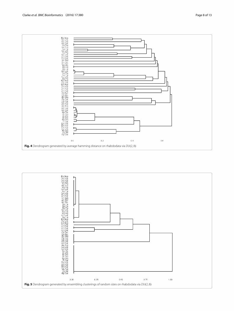
This is the same code as for low dimensional categoricaldata. The resulting dendrogram is in Fig. 4.The dendrogram of the ensemble clustering for rhabdo-

data using hierarchical clustering with average linkage andthe matrix T generated by the B clusterings of the randomsubspaces can be obtained using the following commands.

ens<-enhcHi(rhabdodata$dat,En=100,

len=c(2,8), type=2)

dis0<-hammingD(ens)

REDIST<-as.dist(dis0)

hc1 <- hclust(REDIST,method = "average")

ggdplot(hc1, lab=rhabdodata$lab,

title="average linkage ensembled hclust of

rhabdodata")

enhcHi is the Enscat function that generates I for theequalized length vectors; it stands for ensembling hier-archical clusterings of high dimension. In this example,B = 100 random subspaces are chosen and the values Kbare chosen according to a DUnif [2, 8]. We chose 8 because8 ≈ √

53 and n = 5+ 10+ 16+ 10+ 1+ 3+ 5+ 1+ 2 =53. The argument type=2 specifies a double bootstrapprocedure for variable selection. The result is in Fig. 5.We note that Fig. 5 improves on Fig. 4 in the same sense

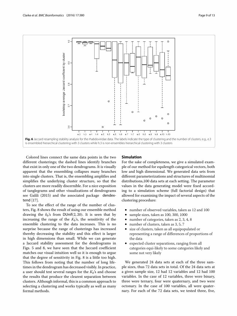
as Fig. 2 improves on Fig. 1. That is, the dendrograms fromthe ensemble methods have an increased number of longlifetimes relative to short lifetimes suggesting increasedstability. Again, this is reflected in the Jaccard coefficientsfor the various choices of K, see Fig. 6. For K = 3, . . . , 8it is clear that the ensemble method gives higher stabil-ity than the hierarchical method though the improvementis not as much as in the low dimensional case for reasonsdiscussed earlier. As a point of interest, note that stabilityindices can themselves become unstable when there is toolittle data per cluster. This is seen for K = 9, 10 in Fig. 6.An alternative way to visualize the improvement pro-

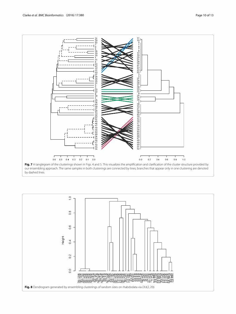
vided by ensembling is shown in the ‘tanglegram’ in Fig. 7.The left hand dendrogram shows the average linkage hier-archical clustering under Hamming distance, while theright hand dendrogram shows the ensembled version ofclusterings of this form. This figure was generated by asimple command,

tangle(hc0, hc1)

Clarke et al. BMC Bioinformatics (2016) 17:380 Page 8 of 13

Fig. 4 Dendrogram generated by average hamming distance on rhabdodata via DU(2, 8)

Fig. 5 Dendrogram generated by ensembling clusterings of random sizes on rhabdodata via DU(2, 8)

Clarke et al. BMC Bioinformatics (2016) 17:380 Page 9 of 13

Fig. 6 Jaccard resampling stability analysis for the rhabdoviridae data. The labels indicate the type of clustering and the number of clusters, e.g., e.3is ensembled hierarchical clustering with 3 clusters while h.3 is non-ensembles hierarchical clustering with 3 clusters

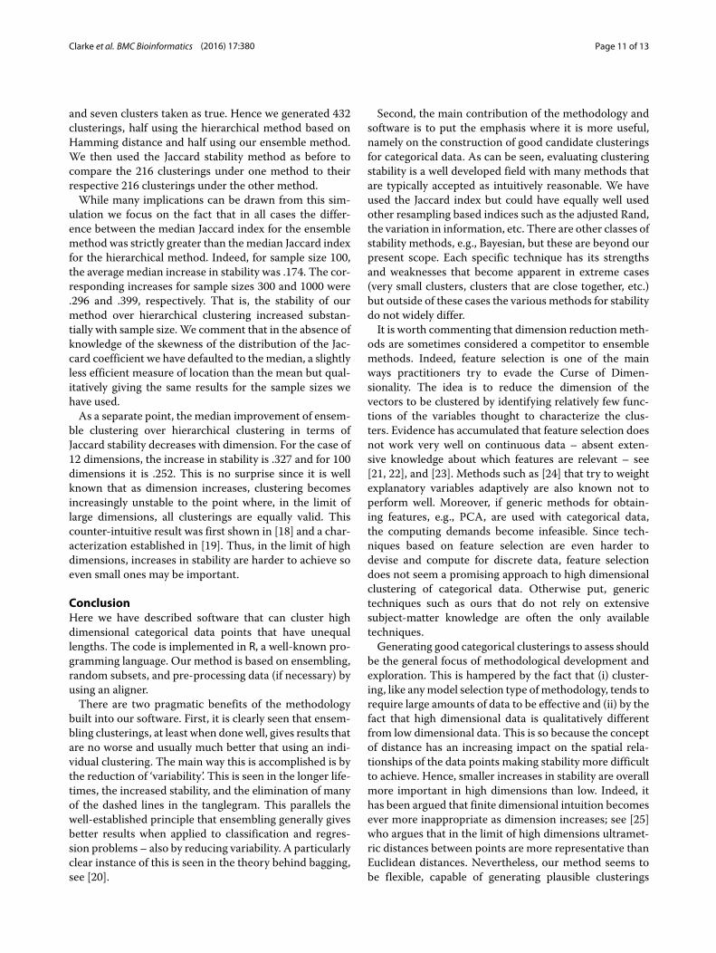
Colored lines connect the same data points in the twodifferent clusterings; the dashed lines identify branchesthat exist in only one of the two dendrograms. It is visuallyapparent that the ensembling collapses many branchesinto single clusters. That is, the ensembling amplifies andsimplifies the underlying cluster structure, so that theclusters are more readily discernible. For a nice expositionof tanglegrams and other visualizations of dendrogramssee Galili (2015) and the associated package dendex-tend [17].To see the effect of the range of the number of clus-

ters, Fig. 8 shows the result of using our ensemble methoddrawing the kb’s from DUnif(2, 20). It is seen that byincreasing the range of the Kb’s, the sensitivity of theensemble clustering to the data increases. This is nosurprise because the range of clusterings has increasedthereby decreasing the stability and this effect is largerin high dimensions than small. While we can generatea Jaccard stability assessment for the dendrograms inFigs. 5 and 8, we have seen that the Jaccard coefficientmatches our visual intuition well so it is enough to arguethat the degree of sensitivity in Fig. 8 is a little too high.This follows from noting that the number of long life-times in the dendrogram has decreased visibly. In practice,a user should test several ranges for the Kb’s and choosethe results that produce the clearest separation betweenclusters. Although informal, this is a common approach toselecting a clustering and works typically as well as manyformal methods.

SimulationFor the sake of completeness, we give a simulated exam-ple of our method for equilength categorical vectors, bothlow and high dimensional. We generated data sets fromdifferent parameterizations and structures of multinomialdistributions,100 data sets at each setting. The parametervalues in the data generating model were fixed accord-ing to a simulation scheme (full factorial design) thatallowed for examining the impact of several aspects of theclustering procedure:

• number of observed variables, taken as 12 and 100• sample sizes, taken as 100, 300, 1000• number of categories, taken as 2, 3, 4, 8• number of clusters, taken as 3, 5, 7• size of clusters, taken as all equipopulated or

representing a range of differences of proportions ofthe data

• expected cluster separations, ranging from allcategories equi-likely to some categories likely andsome not very likely

We generated 24 data sets at each of the three sam-ple sizes, thus 72 data sets in total. Of the 24 data sets ata given sample size, 12 had 12 variables and 12 had 100variables. In the case of 12 variables, three were binary,three were ternary, four were quaternary, and two wereoctonary. In the case of 100 variables, all were quater-nary. For each of the 72 data sets, we tested three, five,

Clarke et al. BMC Bioinformatics (2016) 17:380 Page 10 of 13

Fig. 7 A tanglegram of the clusterings shown in Figs. 4 and 5. This visualizes the amplification and clarification of the cluster structure provided byour ensembling approach. The same samples in both clusterings are connected by lines; branches that appear only in one clustering are denotedby dashed lines

Fig. 8 Dendrogram generated by ensembling clusterings of random sizes on rhabdodata via DU(2, 20)

Clarke et al. BMC Bioinformatics (2016) 17:380 Page 11 of 13

and seven clusters taken as true. Hence we generated 432clusterings, half using the hierarchical method based onHamming distance and half using our ensemble method.We then used the Jaccard stability method as before tocompare the 216 clusterings under one method to theirrespective 216 clusterings under the other method.While many implications can be drawn from this sim-

ulation we focus on the fact that in all cases the differ-ence between the median Jaccard index for the ensemblemethod was strictly greater than the median Jaccard indexfor the hierarchical method. Indeed, for sample size 100,the average median increase in stability was .174. The cor-responding increases for sample sizes 300 and 1000 were.296 and .399, respectively. That is, the stability of ourmethod over hierarchical clustering increased substan-tially with sample size.We comment that in the absence ofknowledge of the skewness of the distribution of the Jac-card coefficient we have defaulted to the median, a slightlyless efficient measure of location than the mean but qual-itatively giving the same results for the sample sizes wehave used.As a separate point, the median improvement of ensem-

ble clustering over hierarchical clustering in terms ofJaccard stability decreases with dimension. For the case of12 dimensions, the increase in stability is .327 and for 100dimensions it is .252. This is no surprise since it is wellknown that as dimension increases, clustering becomesincreasingly unstable to the point where, in the limit oflarge dimensions, all clusterings are equally valid. Thiscounter-intuitive result was first shown in [18] and a char-acterization established in [19]. Thus, in the limit of highdimensions, increases in stability are harder to achieve soeven small ones may be important.

ConclusionHere we have described software that can cluster highdimensional categorical data points that have unequallengths. The code is implemented in R, a well-known pro-gramming language. Our method is based on ensembling,random subsets, and pre-processing data (if necessary) byusing an aligner.There are two pragmatic benefits of the methodology

built into our software. First, it is clearly seen that ensem-bling clusterings, at least when done well, gives results thatare no worse and usually much better that using an indi-vidual clustering. The main way this is accomplished is bythe reduction of ‘variability’. This is seen in the longer life-times, the increased stability, and the elimination of manyof the dashed lines in the tanglegram. This parallels thewell-established principle that ensembling generally givesbetter results when applied to classification and regres-sion problems – also by reducing variability. A particularlyclear instance of this is seen in the theory behind bagging,see [20].

Second, the main contribution of the methodology andsoftware is to put the emphasis where it is more useful,namely on the construction of good candidate clusteringsfor categorical data. As can be seen, evaluating clusteringstability is a well developed field with many methods thatare typically accepted as intuitively reasonable. We haveused the Jaccard index but could have equally well usedother resampling based indices such as the adjusted Rand,the variation in information, etc. There are other classes ofstability methods, e.g., Bayesian, but these are beyond ourpresent scope. Each specific technique has its strengthsand weaknesses that become apparent in extreme cases(very small clusters, clusters that are close together, etc.)but outside of these cases the various methods for stabilitydo not widely differ.It is worth commenting that dimension reductionmeth-

ods are sometimes considered a competitor to ensemblemethods. Indeed, feature selection is one of the mainways practitioners try to evade the Curse of Dimen-sionality. The idea is to reduce the dimension of thevectors to be clustered by identifying relatively few func-tions of the variables thought to characterize the clus-ters. Evidence has accumulated that feature selection doesnot work very well on continuous data – absent exten-sive knowledge about which features are relevant – see[21, 22], and [23]. Methods such as [24] that try to weightexplanatory variables adaptively are also known not toperform well. Moreover, if generic methods for obtain-ing features, e.g., PCA, are used with categorical data,the computing demands become infeasible. Since tech-niques based on feature selection are even harder todevise and compute for discrete data, feature selectiondoes not seem a promising approach to high dimensionalclustering of categorical data. Otherwise put, generictechniques such as ours that do not rely on extensivesubject-matter knowledge are often the only availabletechniques.Generating good categorical clusterings to assess should

be the general focus of methodological development andexploration. This is hampered by the fact that (i) cluster-ing, like anymodel selection type ofmethodology, tends torequire large amounts of data to be effective and (ii) by thefact that high dimensional data is qualitatively differentfrom low dimensional data. This is so because the conceptof distance has an increasing impact on the spatial rela-tionships of the data points making stability more difficultto achieve. Hence, smaller increases in stability are overallmore important in high dimensions than low. Indeed, ithas been argued that finite dimensional intuition becomesever more inappropriate as dimension increases; see [25]who argues that in the limit of high dimensions ultramet-ric distances between points are more representative thanEuclidean distances. Nevertheless, our method seems tobe flexible, capable of generating plausible clusterings

Clarke et al. BMC Bioinformatics (2016) 17:380 Page 12 of 13

when used reasonably, and amenable to stability assess-ments for finite dimensions.We conclude by noting that even in the simplest case –

clustering low dimensional categorical data having equallengths – no previous method can be regarded as well-established. However, in [7], we have argued theoreticallyand by examples that the method implemented by oursoftware performs better on average than many otherclustering methods in settings where other methods exist.We have also argued that in the case of fixed length highdimensional clustering our method outperforms mixedweighted K-modes, a technique from [26]. In the case ofnon-fixed length high dimensional data, we have com-pared our method to phylogenetic trees developed frombiomarkers. Our method appears to give results thatare equally or slightly more accurate and more generallyattainable since they do not rest on biological informationthat is often not available.

Availability and requirementsProject name: EnsCat.Project home page: https://github.com/jlp2duke/EnsCatOperating systems:Windows, OS X.Programming language: R ≥ 3.2.4.Other requirements: aligner (for unequal length data).License: GNU, GPL.Any restrictions to use by non-academics: None.

Endnotes1 The principle of insufficient reason states that one

should assign a uniform value across elements in theabsence of reason to do otherwise.

2 In hierarchical clustering a ‘linkage’ function must bedefined. A linkage function represents a distance or sumof distances from any given point set to another point set.Single linkage means the shortest distance between thetwo point sets. Complete linkage means the longest dis-tance between two point sets. Average linkage means theaverage of all the distances between the points in the twosets. There are other linkage functions that are used butthese two are the most common.

3 The commands are given in the manual at https://github.com/jlp2duke/EnsCat.

AbbreviationsDUnif: Uniform distribution; IID: Independent and identically distributed;MBC: Model based clustering; PCA: Principal components analysis; ViPR: VirusPathogen Database and Analysis Resource

AcknowledgmentsThe authors express their gratitude to the anonymous reviewers for theirexcellent comments and suggestions. The authors thank the University ofNebraska Holland Computing Center for essential computational support.

FundingThis research was supported by the National Science Foundation under awardDMS-1120404. The content is solely the responsibility of the authors and doesnot necessarily represent the official views of the National Science Foundation.

Availability of data andmaterialsThe software, user manual, data, and supporting materials can be downloadedfrom https://github.com/jlp2duke/EnsCat.

Authors’ contributionsBSC, SA, and JLC carried out the implementation and evaluation of theproposed method, participated in the software design and evaluation anddrafted the manuscript. All authors read and approved the final manuscript.

Competing interestsThe authors declare that they have no competing interests.

Consent for publicationNot applicable.

Ethics approval and consent to participateNot applicable.

Author details1Department of Statistics, University of Nebraska-Lincoln, Lincoln, NE, USA.2Department of Natural and Applied Sciences, University of WisconsinMadison, Iowa City, IA, USA. 3Department of Food Science and Technology,University of Nebraska-Lincoln, Lincoln, NE, USA.

Received: 21 May 2016 Accepted: 8 September 2016

References1. Huang Z. Extensions to the v-means algorithm for clustering large data

sets with categorical values. Data Min Knowl Disc. 1998;2:283–304.2. Celeux G, Govaert G. Clustering criteria for discrete data and latent class

models. J Classif. 1991;8(2):157–76.3. Guha S, Rastogi R, Shim K. ROCK: A robust clustering algorithm for

categorical attributes. Inf Syst. 2000;25(5):345–66.4. Zaki M, Peters M, Assent I, Seidl T. Click: An effective algorithm for

mining subspace clusters in categorical datasets. Data Knowl Eng.2007;60(1):51–70.

5. Topchy A, Jain A, Punch W. Clustering ensembles: Models of consensusand weak partitions. Pattern Anal Mach Intell. 2005;27(12):1866–81.

6. Wilkerson M, Hayes D. Consensusclusterplus: a class discovery tool withconfidence assessments and item tracking. Bioinformatics. 2010;26:1572–3.

7. Amiri S, Clarke J, Clarke B. Clustering categorical data via ensemblingdissimilarity matrices. 2015. http://arxiv.org/abs/1506.07930. Accessed 12Sept 2016.

8. Tabakis E. Robust Statistics, Data Analysis, and Computer IntensiveMethods: In Honor of Peter Huber’s 60th Birthday In: Rieder H, editor.Lecture Notes in Statistics. New York: Springer; 1996. p. 375–89.

9. Yeung K, Ruzzo W. Principal component analysis for clustering geneexpression data. Bioinformatics. 2001;17(9):763–74.

10. R Core Team. R: A Language and Environment for Statistical Computing.Vienna: R Foundation for Statistical Computing; 2016. R Foundation forStatistical Computing. http://www.R-project.org. Accessed 12 Sept 2016.

11. Breiman L. Random forests. Mach Learn. 2001;45(1):5–32.12. United States Maritime Administration. MARAD open data portal –

maritime data and statistics, u.s.-flag privately-owned fleet (as of3/3/2016). PhD thesis, United States Department of Transportation. 2016.http://marad.dot.gov/resources/data-statistics/. Accessed 25 Mar 2016.

13. Amiri S, Clarke B, Clarke J, Koepke H. A general hybrid clusteringtechnique. 2015. http://arxiv.org/abs/1503.01183. Accessed 12 Sept 2016.

14. Hennig C. Cluster-wise assessment of cluster stability. Comput Stat DataAnal. 2007;52:258–71.

15. Pickett BE, Sadat EL, Zhang Y, Noronha JM, Squires RB, Hunt V, Liu M,Kumar S, Zaremba S, Gu Z, Zhou L, Larson CN, Dietrich J, Klem EB,Scheuermann RH. ViPR: an open bioinformatics database and analysis

Clarke et al. BMC Bioinformatics (2016) 17:380 Page 13 of 13

resource for virology research. Nuc Acids Res. 2012;40(D1):593–8.Accessed 27 Apr 2015.

16. Katoh K, Standley D. MAFFT multiple sequence alignment softwareversion 7: improvements in performance and usability. Mol Biol Evol.2013;30(4):772–80. Accessed 2 Mar 2015.

17. Galili T. dendextend: an r package for visualizing, adjusting, andcomparing trees of hierarchical clustering. Bioinformatics. 2015.doi:10.1093/bioinformatics/btv428. http://bioinformatics.oxfordjournals.org/content/31/22/3718.full.pdf+html.

18. Beyer K, Goldstein R, Ramakrishnan R, Shaft U. When is ‘nearestneighbor’ meaningful?. In: Proceedings of the 7th InternationalConference on Database Theory; 1999. p. 217–35.

19. Koepke H, Clarke B. On the limits of clustering in high dimensions via costfunctions. Stat Anal Data Mining. 2011;4(1):30–53.

20. Breiman L. Bagging predictors. Technical Report No. 421, Department ofStatistics, University of California Berkley. 1994.

21. Yeung K, Ruzzo W. Principal component analysis for clustering geneexpression data. Bioinformatics. 2001;17(9):763–74.

22. Chang W. On using principal components before separating a mixture oftwo multivariate normal distributions. Appl Stat. 1983;32(3):267–75.

23. Witten D, Tibshirani R. A framework for feature selection in clustering.J Amer Stat Assoc. 2010;105:713–26.

24. Friedman J, Meulman J. Clustering objects on subsets of attributes. J RoyStat Soc Ser B. 2004;66:815–49.

25. Murtagh F. On ultrametricity, data coding, and computation. J Class.2004;21(2):167–84.

26. Bai L, Liang J, Dang C, Cao F. A novel attribute weighting algorithm forclustering high-dimensional categorical data. Pattern Recogn.2011;44(12):2843–61.

• We accept pre-submission inquiries

• Our selector tool helps you to find the most relevant journal

• We provide round the clock customer support

• Convenient online submission

• Thorough peer review

• Inclusion in PubMed and all major indexing services

• Maximum visibility for your research

Submit your manuscript atwww.biomedcentral.com/submit

Submit your next manuscript to BioMed Central and we will help you at every step: