enhancing the utility of daily gcm rainfall for crop yield

INTERNATIONAL JOURNAL OF CLIMATOLOGYInt. J. Climatol. (2010)Published online in Wiley Online Library(wileyonlinelibrary.com) DOI: 10.1002/joc.2223

Enhancing the utility of daily GCM rainfall for crop yieldprediction

Amor V. M. Ines,* James W. Hansen and Andrew W. RobertsonInternational Research Institute for Climate and Society, The Earth Institute at Columbia University, Palisades, NY 10964-8000, USA

ABSTRACT: Global climate models (GCMs) are promising for crop yield predictions because of their ability to simulateseasonal climate in advance of the growing season. However, their utility is limited by unrealistic time structure of dailyrainfall and biases in rainfall frequency and intensity distributions. Crop growth is very sensitive to daily variations ofrainfall; thus any mismatch in daily rainfall statistics could impact crop yield simulations. Here, we present an improvedmethodology to correct GCM rainfall biases and time structure mismatches for maize yield prediction in Katumani, Kenya.This includes GCM bias correction (BC), to correct over- or under-predictions of rainfall frequency and intensity, andnesting corrected GCM information with a stochastic weather generator, to generate daily rainfall realizations conditionedon a given monthly target. Bias-corrected daily GCM rainfall and generated rainfall realizations were used to evaluate cropresponse. Results showed that corrections of GCM rainfall frequency and intensity could improve crop yield prediction butyields remain under-predicted. This is strongly attributed to the time structure mismatch in daily GCM rainfall leading toexcessively long dry spells. To address this, we tested several ways of improving daily structure of GCM rainfall. First, wetested calibrating thresholds in BC but were found not very effective for improving dry spell lengths. Second, we testedBC-stochastic disaggregation (BC-DisAg) and appeared to simulate more realistic dry spell lengths using bias-correctedGCM rainfall information (e.g., frequency, totals) as monthly targets. Using rainfall frequency alone to condition theweather generator removed biases in dry spell lengths, improved predicted yields, but under-predicted yield variability.Combining rainfall frequency and totals, however, not only produced more realistic yield variability but also correctedunder-prediction of yields. We envisaged that the presented method would enhance the utility of daily GCM rainfall incrop yield prediction. Copyright 2010 Royal Meteorological Society

KEY WORDS bias correction; GCM; crop models; weather generator; stochastic disaggregation

Received 4 June 2010; Revised 3 August 2010; Accepted 7 August 2010

1. Introduction

Translating seasonal climate forecasts into crop yieldresponse is crucial for food security planning and man-agement as they provide useful information for decisionmakers to formulate decisions in advance of food inse-curity outlooks (Challinor et al., 2005; Hansen et al.,2006). Linking climate forecasts with crop models isoften the method used for forecasting crop yields (Hansenand Indeje, 2004; Hansen and Ines, 2005; Semenov andDoblas-Reyes, 2007; Mishra et al., 2008). The procedure,however, is not straightforward because of mismatchbetween the time structure of climate data required bycrop simulation models and the temporal resolution of cli-mate forecasts. Crop models usually require daily weatherinputs for simulating crop growth (Tsuji et al., 1994;Jones et al., 2003) while climate forecasts are typicallymade for seasonal time scale (typically 3 months) (God-dard et al., 2001; Goddard and Mason, 2002). Recentprogress in addressing this problem includes linking sea-sonal climate forecasts with stochastic weather generators

* Correspondence to: Amor V. M. Ines, International Research Insti-tute for Climate and Society, The Earth Institute at Columbia Univer-sity, Palisades, NY 10964-8000, USA. E-mail: [email protected]

to generate daily rainfall sequences, then used as inputsto crop simulation models (Hansen and Indeje, 2004;Hansen and Ines, 2005; Robertson et al., 2007; Semenovand Doblas-Reyes, 2007; Mishra et al., 2008).

Daily outputs from global or regional climate modelshave been proposed for bridging the gap between cropsimulation models and seasonal climate forecasts (Hansenand Indeje, 2004). Dynamic climate models run inforecast mode could easily provide the daily data requiredby crop simulation models. However, linking daily GCMrainfall with crop models is not also as straightforwardas it seems because of the biases in GCM rainfallrelative to station data. Biases in rainfall statistics mustbe first corrected before linking them with crop modelsas distortions in rainfall frequency and intensity couldadversely impact the simulation of crop growth andyield, resulting in unrealistic outcomes (Mearns et al.,1996; Riha et al., 1996; Mavromatis and Jones, 1999;Hansen and Jones, 2000; Baron et al., 2005). Devisingways for extracting and refining information from dailyGCM rainfall for crop simulations are crucial for theirsuccessful applications in crop yield predictions.

Ines and Hansen (2006) developed a bias correction(BC) method for daily GCM rainfall for correcting

Copyright 2010 Royal Meteorological Society

A. V. M. INES et al.

biases in rainfall frequency, intensity and totals relativeto a station inside a grid cell. They used a two-step approach by correcting rainfall frequency, then theintensity distribution. Rainfall frequency was correctedby truncating the cumulative distribution function (CDF)of daily GCM rainfall from the observation distributionabove a calibrated threshold. Mapping the quantiles of thetruncated daily GCM rainfall CDF onto the observationswas used to correct rainfall intensity. As rainfall totalis the product of frequency and intensity, correctingboth the biases of intensity and frequency will correctrainfall total bias. Schmidli et al. (2006) also proposeda slightly varied method for correcting daily GCMrainfall biases. They used a wet-day threshold to matchobserved and model rainfall frequency, similar to Inesand Hansen (2006), and a scaling factor, based on theratio between wet-day intensities of observations andadjusted GCM rainfall, to correct rainfall intensity. Arecent comparison between the two methods can be seenin Dobler and Ahrens (2008). GCM BC has been usedin other applications as well (e.g. Sharma et al., 2007;Elshamy et al., 2009; Mishra and Singh, 2009; Mishraet al., 2009) aside from agro-meteorological applications(Baigorria et al., 2007, 2008).

Bias-corrected daily GCM rainfall used as input tocrop simulation models has made improvements inpredicted yields compared to using raw daily GCMrainfall alone (Hansen et al., 2006). Ines and Hansen(2006) observed, however, that a significant bias (neg-ative) in the predicted yields still exists after BCs ofdaily GCM rainfall. Their analysis suggests that thetime structure of daily GCM rainfall does not corre-spond well with station data and that daily GCM rain-fall tends to overestimate dry spell lengths (here, ≤1mm = dry day) exposing the crops to longer periodsof dry spells, thus reducing yields. The deterministicGCM BC was not able to correct this bias in dry spelllengths.

The general purpose of this article is to test the notionthat by improving the daily structure of GCM rainfall

(in bias-corrected or in derived form), the predictedyields by crop simulation models can be improvedfurther. Specifically, we aim (1) to explore strategiesfor improving the time structure of bias-corrected dailyGCM rainfall and (2) to evaluate the performance of theimproved daily GCM rainfall for crop yield predictions.We tested the methods in an agricultural experimentalstation in Katumani, Machakos district of eastern Kenya,using maize as a case study.

2. Materials and methods

2.1. Climate data

We used ECHAMv4.5 (Roeckner et al., 1996) simu-lated daily rainfall forced by concurrent observed sea-surface temperature (SST) (http://iridl.ldeo.columbia.edu)for BC and crop yield prediction. Note that a GCMrun in historical mode delineates the upper boundof climate predictability and that predictive skill inforecast mode (i.e. forced by forecast SSTs) may belesser than this level (Challinor et al., 2005). For pur-poses of testing and demonstration, we chose modelruns in historical mode. Here, we expanded the studydomain considered by Ines and Hansen (2006) froma single to multiple grid cells to test if multi-gridGCM cells can provide better information for cropyield prediction. We selected 3 × 3 model grid cells(1°23.7′N–4°10.8′S, 33°45′E–39°20.5′E) encompassingthe Katumani Dryland Research Center (1°35′S, 37°14′E)(Table I, Figure 1) wherein all 24 ensemble members(GCM simulations from different initial conditions) ineach grid cell considered were extracted for analy-sis for the study period (1970–1995). Rainfall in thisregion is bi-modal, occurring in February–May and Octo-ber–December. The latter shorter rainy season is animportant maize growing season in the region whose pre-dictability potential has been established in recent studies(e.g. Indeje et al., 2000; Hansen and Indeje, 2004). Dailyrainfall observations and other weather data needed for

Table I. Geographic locations, distance from station, weights and uncorrected yield correlations of the selected ECHAMv4.5 gridcells.

Location Longitude Latitude Distance, r

(degrees)Weight, ω (r)(degrees−2)

Uncorrected yield R

(−) and MBE (Mg ha−1,in parenthesis)

Corrected yield† R

(−) and MBE (Mg ha−1,in parenthesis)

Station 37°14′E 1°35′S 0.000 Null Null NullGrid1 33°45′E 4°11.16′S 4.348 0.053 0.60 (−0.32) 0.61 (−0.18)Grid2 36°33.75′E 4°11.16′S 2.688 0.138 0.68 (−2.18) 0.71 (−0.85)Grid3 39°22.5′E 4°11.16′S 3.371 0.088 0.43 (−2.84) 0.36 (−0.62)Grid4 33°45′E 1°23.72′S 3.488 0.082 0.04 (0.76) 0.67 (−0.20)Grid5 36°33.75′E 1°23.72′S 0.697 2.060 0.61 (−2.35) 0.70 (−0.90)Grid6 39°22.5′E 1°23.72′S 2.150 0.216 0.44 (−3.13) 0.38 (−0.30)Grid7 33°45′E 1°23.72′N 4.583 0.048 0.40 (0.52) 0.58 (−0.15)Grid8 36°33.75′E 1°23.72′N 3.053 0.107 0.65 (−2.10) 0.61 (−0.70)Grid9 39°22.5′E 1°23.72′N 3.669 0.074 0.59 (−3.17) 0.45 (−0.34)

† Using the new bias correction approach, BC2 (>0 mm threshold; Section 2.2.1).

Copyright 2010 Royal Meteorological Society Int. J. Climatol. (2010)

ENHANCING THE UTILITY OF DAILY GCM RAINFALL

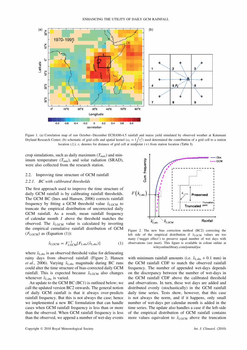
Figure 1. (a) Correlation map of raw October–December ECHAMv4.5 rainfall and maize yield simulated by observed weather at KatumaniDryland Research Center; (b) schematic of grid cells and spatial kernel (ωi = 1

/r2i ) used determined the contribution of a grid cell to a station

location (�); ri denotes for distance of grid cell at midpoint (+) from station location (Table I).

crop simulations, such as daily maximum (Tmax) and min-imum temperature (Tmin), and solar radiation (SRAD),were also collected from the research station.

2.2. Improving time structure of GCM rainfall

2.2.1. BC with calibrated thresholds

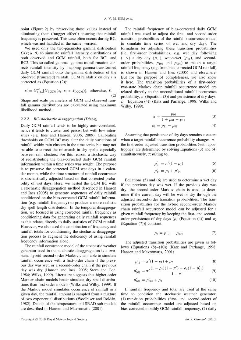
The first approach used to improve the time structure ofdaily GCM rainfall is by calibrating rainfall thresholds.The GCM BC (Ines and Hansen, 2006) corrects rainfallfrequency by fitting a GCM threshold value xI,GCM totruncate the empirical distribution of uncorrected dailyGCM rainfall. As a result, mean rainfall frequencyof calendar month I above the threshold matches theobserved. The xI,GCM value is calculated by invertingthe empirical cumulative rainfall distribution of GCM(FI,GCM) as (Equation (1)):

xI,GCM = F −1I,GCM[FI,obs(xI,obs)] (1)

where xI,obs is an observed threshold value for delineatingrainy days from observed rainfall (Figure 2; Hansenet al., 2006). Varying xI,obs magnitude during BC runscould alter the time structure of bias-corrected daily GCMrainfall. This is expected because xI,GCM also changeswhenever xI,obs is varied.

An update to the GCM BC (BC1) is outlined below; wecall the updated version BC2 onwards. The general notionof daily GCM rainfall is that it always over-predictsrainfall frequency. But this is not always the case; hencewe implemented a new BC formulation that can handlecases when GCM rainfall frequency is less than or morethan the observed. When GCM rainfall frequency is lessthan the observed, we append a number of wet-day events

Figure 2. The new bias correction method (BC2) correcting theleft side of the empirical distribution if xI,GCM values are toomany (‘nugget effect’) to preserve equal number of wet days withobservations (see inset). This figure is available in colour online at

wileyonlinelibrary.com/journal/joc

with minimum rainfall amounts (i.e. xI,obs + 0.1 mm) inthe GCM rainfall CDF to match the observed rainfallfrequency. The number of appended wet-days dependson the discrepancy between the number of wet-days inthe GCM rainfall CDF above the calibrated thresholdand observations. In turn, these wet days are added anddistributed evenly (stochastically) in the GCM rainfalldaily time series. Tests show, however, that this caseis not always the norm, and if it happens, only smallnumber of wet-days per calendar month is added in thetime series. The update also handles a case if the left-sideof the empirical distribution of GCM rainfall containsmore values equivalent to xI,GCM above the truncation



point (Figure 2) by preserving those values instead ofeliminating them (‘nugget effect’) ensuring that rainfallfrequency is preserved. This case often occurs during BC,which was not handled in the earlier version.

We used only the two-parameter gamma distributionG(x; α, β) to simulate rainfall intensity distributions ofboth observed and GCM rainfall, both for BC1 andBC2. This so-called gamma–gamma transformation cor-rects rainfall intensity by mapping gamma-transformeddaily GCM rainfall onto the gamma distribution of theobserved (truncated) rainfall. GCM rainfall x on day i iscorrected as (Equation (2)):

x ′i = G−1

I,obs[GI,GCM(xi; xi > xI,GCM)], otherwise, 0.

(2)

Shape and scale parameters of GCM and observed rain-fall gamma distributions are calculated using maximumlikelihood method.

2.2.2. BC-stochastic disaggregation (DisAg)

Daily GCM rainfall tends to be highly auto-correlated,hence it tends to cluster and persist but with low inten-sities (e.g. Ines and Hansen, 2006, 2009). Calibratingthresholds on GCM BC may alter the daily variations ofrainfall within rain clusters in the time series but may notbe able to correct the mismatch in dry spells especiallybetween rain clusters. For this reason, a stochastic wayof redistributing the bias-corrected daily GCM rainfallinformation within a time series was sought. The purposeis to preserve the corrected GCM wet days in a calen-dar month, while the time structure of rainfall occurrenceis stochastically adjusted based on that corrected proba-bility of wet days. Here, we nested the GCM BC witha stochastic disaggregation method described in Hansenand Ines (2005) to generate sequences of daily rainfallconditioned on the bias-corrected GCM rainfall informa-tion (e.g. rainfall frequency) to produce a more realisticdry spell length distribution. In the temporal disaggrega-tion, we focused in using corrected rainfall frequency asconditioning data for generating daily rainfall sequencesas this relates directly to daily statistics of GCM rainfall.However, we also used the combination of frequency andrainfall totals for conditioning the stochastic disaggrega-tion process to augment the deficiency of using rainfallfrequency information alone.

The rainfall occurrence model of the stochastic weathergenerator used in the stochastic disaggregation is a two-state, hybrid second-order Markov chain able to simulaterainfall occurrence with a first-order chain if the previ-ous day was wet, or a second-order chain if the previousday was dry (Hansen and Ines, 2005; Stern and Coe,1984; Wilks, 1999). Literature suggests that higher orderMarkov chain models better simulate dry spell distribu-tions than first-order models (Wilks and Wilby, 1999). Ifthe Markov model simulates occurrence of rainfall in agiven day, the rainfall amount is sampled from a mixtureof two exponential distributions (Woolhiser and Roldan,1982). Details of the temperature and SRAD sub-modelsare described in Hansen and Mavromatis (2001).

The rainfall frequency of bias-corrected daily GCMrainfall was used to adjust the first- and second-ordertransition probabilities of the rainfall occurrence modelto simulate time series of wet and dry days. Theformalism for adjusting these transition probabilities(i.e. first-order probabilities, e.g. wet day following(−>) a dry day (p01), wet->wet (p11), and second-order probabilities, p101 and p001) to match a targetrainfall frequency (e.g. from bias-corrected GCM rainfall)is shown in Hansen and Ines (2005) and elsewhere.But for the purpose of completeness, we also showit here. The transition probabilities of a first-order,two-state Markov chain rainfall occurrence model arerelated directly to the unconditional rainfall occurrenceprobability, π (Equation (3)) and persistence of dry days,ρ1 (Equation (4)) (Katz and Parlange, 1998; Wilks andWilby, 1999).

π = p01

1 + p01 − p11(3)

ρ1 = p11 − p01 (4)

Assuming that persistence of dry days remains constantwhen a target rainfall occurrence probability changes, π ′,the first-order adjusted transition probabilities (with apos-trophes) are determined by solving Equations (3) and (4)simultaneously, resulting to,

p′01 = π ′(1 − ρ1) (5)

p′11 = ρ1 + p′

01 (6)

Equations (5) and (6) are used to determine a wet dayif the previous day was wet. If the previous day wasdry, the second-order Markov chain is used to deter-mine if the current day will be wet or dry through theadjusted second-order transition probabilities. The tran-sition probabilities for the hybrid second-order Markovchain rainfall occurrence model can be adjusted for agiven rainfall frequency by keeping the first- and second-order persistence of dry days [ρ1 (Equation (4)) and ρ2

(Equation (7))] constant.

ρ2 = p101 − p001 (7)

The adjusted transition probabilities are given as fol-lows (Equations (8)–(10)) (Katz and Parlange, 1998;Hansen and Mavromatis, 2001)

p′11 = π ′(1 − ρ1) + ρ2 (8)

p′001 = π ′ (1 − ρ1)(1 − π ′) − ρ2(1 − p′

11)

1 − π ′ (9)

p′101 = p′

001 + ρ2 (10)

If rainfall frequency and total are used at the sametime to condition the stochastic weather generator,(1) transition probabilities (first- and second-order) ofthe rainfall occurrence model are adjusted based onbias-corrected monthly GCM rainfall frequency, (2) daily



Table II. Summary descriptions of methods used in this study.

Methods Descriptions

BC1 Based on Ines and Hansen (2006), corrects rainfall frequency (under-prediction) by truncating GCM rainfalldistribution at a given threshold, corrects rainfall intensity using gamma–gamma transformation

BC1-DisAg1 BC1 combined with stochastic disaggregation (DisAg) conditioned on the corrected rainfall frequency of eachensemble member, respectively

BC1-DisAg2 BC1 combined with DisAg conditioned on the corrected average rainfall frequency from all ensemble membersBC2 Corrects rainfall frequency (under- and over-prediction) by truncating the GCM rainfall distribution at a given

threshold, and also corrects the ‘nugget effect’ of truncating empirical distribution (Figure 2). Corrects rainfallintensity using gamma–gamma transformation

BC2-DisAg1 BC2 combined with DisAg conditioned on the corrected rainfall frequency of each ensemble member,respectively

BC2-DisAg2 BC2 combined with DisAg conditioned on the corrected average rainfall frequency from all ensemble membersBC2-m BC2 applied to multiple grid cellsBC2-DisAg2-m BC2 combined with DisAg conditioned on the corrected average rainfall frequency (and amounts) from all

multiple grid cells

rainfall realizations are generated iteratively until gen-erated monthly rainfall total matches 95% of the tar-get value (the bias-corrected monthly GCM rainfall),(3) generated daily values are re-scaled by a ratio ofmonthly target (Rm) and generated rainfall totals (Rm)(i.e. Rm/Rm) such that the monthly rainfall total gen-erated matches the target value. These three steps arerepeated in turn, for each calendar month in a year, forall the years considered (Hansen and Ines, 2005).

2.3. Case studies for BC and BC-stochasticdisaggregation

Table II shows a summary of the experiments performedin this study. First, we considered a single ECHAMv4.5grid cell encompassing the agricultural research station(Figure 1) to compare the performances of BC1 andBC2. The 24 ensemble members were individually bias-corrected using several observed threshold values (>0, 1,3 and 5 mm). Monthly rainfall statistics from the bias-corrected daily GCM rainfall were extracted for linkingto stochastic disaggregation. In the single grid cell case,only the monthly time series of rainfall frequency (π)was used to condition the stochastic weather generator(as this can directly represent the daily GCM rainfallstatistics), (1) for each ensemble member (BC-DisAg1)and (2) aggregated 24 members (BC-DisAg2), where BCis the general term for GCM bias correction (BC) andDisAg for stochastic disaggregation.

The second case involves multiple grid cells fromECHAMv4.5 where all nine grid cells selected were usedin the analysis (Figure 1). Using only now, the new BCformulation (BC2), the 24 ensemble members from eachGCM grid cell were bias-corrected individually, thenanalysed to extract monthly rainfall statistics. As will beshown later, individual ensemble member contains lesserinformation than when combined with other ensemblemembers in the GCM run. Therefore, we used onlythe aggregated monthly rainfall frequency, and rainfalltotals, for each grid cell to develop a grid-based monthlytime series of rainfall frequency and totals for stochastic

disaggregation. This was done using a simple spatialkernel given below (Equations (11)–(13); Figure 1(b)).

πt =

N∑i=1

ωiπit

N∑i=1

ωi

∀t (11)

ωi = 1

r2i

(12)

ri =√

(xi − xstation)2 + (yi − ystation)2 (13)

where π is the weighted conditioning data (e.g. fre-quency, totals), ω is a weighting function, r is the gridcell distance from the weather station, x and y are lon-gitude and latitude, i is an index of grid cell, t an indexfor time (i.e. months, for 26 years), and N is the num-ber of grid cells. We also used arithmetic averaging (allgrid cells have the same weights) for developing the grid-based conditioning data for stochastic disaggregation.

We generated 24 realizations of daily rainfall for allthe BC-stochastic disaggregation experiments. The 24realizations were replicated ten times to minimize thevariability of small samples in stochastic modelling.The 24-realization run was chosen for the stochasticdisaggregation to give a better basis for comparison withthe BC runs applied to 24 ensemble members.

As will be shown in Section 2.4, we linked the cor-rected information with a crop simulation model. Thisrequires that the corrected daily GCM rainfall must becoupled with other weather variables considering theirdependency with rainfall. There are several ways to sat-isfying this requirement. Baigorria et al. (2007) suggestedbias correcting climate model’s daily temperature (T ) andSRAD in addition to rainfall for inputs to crop yield pre-diction. This approach attempts to ensure that T andSRAD are consistent with rainfall, but since they arebias-corrected independently, a perfect dependency with



rainfall is not always guaranteed in the end. This can beapplied using BC alone. We can also use the weathergenerator to generate daily realizations of temperature(Tmin and Tmax) and SRAD conditioned on the time seriesof bias-corrected GCM rainfall. In this study, however,we opted for a simpler approach. For all BC and BC-DisAg runs, daily Tmin, Tmax and SRAD were generatedas monthly mean values conditioned on the occurrence ornonoccurrence of rainfall. In other words, if the currentday is wet, we used the wet-day mean values of Tmin,Tmax and SRAD of that month as values on that partic-ular day, vice versa. This is analogous to filling missingdata with mean + noise, with noise = 0 and the mean isa conditional value. Conditioning the values on a wet ordry day occurrence preserves the co-variation of rainfallwith other weather variables. Our earlier tests show thatthis approximation resulted to yields comparable to thosesimulated with actual weather.

2.4. Linking daily GCM rainfall with a crop model

The performance of BC and BC-DisAg outputs werequantitatively evaluated by linking them to a crop simula-tion model. We used CERES-Maize (Ritchie et al., 1998)to simulate and predict maize yields. Data inputs on soilproperties, local cultivar ‘Katumani composite B ’ char-acteristics and management assumptions were based ona previous study at the same site (Keating et al., 1992).The sandy clay loam soil used in the crop modelling hasplant-extractable water-holding capacity of 180 mm m−1

of soil. For each simulation year, the soil-water balancewas initialized on 17 October with initial soil moistureat 20% water-holding capacity. Sowing was establishedby the CERES-Maize and was simulated once the soilmoisture content of the top 15 cm soil surface exceeded40% of water-holding capacity. If sowing fails within theprescribed window, sowing will commenced forcedly on1 November. The plant density was assumed to be 4.4plants m−2 with 50 cm row spacing and 20 kg N ha−1

applied as ammonium nitrate (NH4NO3) at sowing. Otherdetails are described in Ines and Hansen (2006).

CERES-Maize was run with observed daily rainfall(>0 mm threshold) for baseline, daily rainfall fromECHAMv4.5 without BC, with BC (all thresholds, >0,1, 3, 5 mm) under BC1 and BC2, and with variants ofBC (all thresholds) - stochastic disaggregation (Table II).Simulated yields for individual years were averagedacross the 24 GCM ensemble members and from the24 realizations (replicated ten times) by the stochasticdisaggregation, then compared with the baseline yields.To ensure that yields are simulated with consistenttemperature and SRAD, we used the conditional meanvalues of Tmin, Tmax and SRAD in the baseline simulationin lieu of the observed values.

2.5. Analysis of results

Standard goodness-of-fit statistics was used to analysemodel performances. We decomposed the mean squared

error (Equation (14)) into a random component (not cor-rected by linear regression) (Equation (15)) and a system-atic component (can be corrected by linear regression)(Equation (16)) based on Willmott (1982),

MSE = 1

n

n∑i=1

(yi − yi)2 (14)

MSER = 1

n

n∑i=1

(y∗i − yi)

2 (15)

MSES = MSE − MSER (16)

where n is the number of years, i, y and y are yieldssimulated with observed and uncorrected/corrected GCMrainfall, y∗ is y calibrated by linear regression. We alsoused correlation coefficient (R), mean bias error (MBE),root-mean-squared error (RMSE) and index of agreementd-statistics (Equation (17)) to measure performance,where y is average observed yields.

d = 1 −

n∑i=1

(yi − yi)2

n∑i=1

(|yi − y| + |yi − y|)2

. (17)

Aside from yields, goodness-of-fit statistics for bias-corrected and generated GCM-based rainfall were cal-culated to evaluate the performance of the enumeratedmethods for enhancing the utility of daily GCM rain-fall for crop yield prediction. Of particular interest isthe evaluation of dry spell lengths among methods, asthis was suggested to be the major influencing factor forthe underestimation of yields when linking daily GCMrainfall with crop simulation models.

3. Results and discussions

3.1. Crop yield predictions

3.1.1. Without BC

Due to lack of available actual yield data, we optedto pursue the analysis with maize yields simulatedby observed weather, with the exception of temper-ature and SRAD values (Section 2.4). ECHAMv4.5October–December (raw) rainfall is moderately–high-ly correlated with the baseline yield (Figure 1(a)). Thisis interesting to note because it suggests the goodpredictability of maize yields in the region.

Figure 3 shows the predicted yields using uncorrecteddaily GCM rainfall from the selected 3 × 3 grid cells.Except for grid cell 4 (Figure 1(b)), a moderate to strongcorrelation (0.40–0.68, Table I) exists between yieldssimulated by observed station rainfall and those simulatedby uncorrected GCM rainfall from surrounding grid cells,suggesting that the inter-annual variability of rainfallwas more or less captured by the climate model for themajority of grid cells selected, as evident in Figure 1(a).



But most of the yields simulated by uncorrected dailyGCM rainfall extremely under-predicted those simulatedby observed station rainfall (Table I, MBE uncorrected).This can be explained in part by the rainfall characteris-tics of the selected grid cells. The seasonal rainfall (Octo-ber–December) was extremely underestimated (Table III,uncorrected).

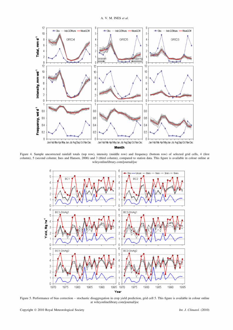
For comparison purposes, we selected three grid cellsrepresenting the three clusters of simulated yield levels(Figure 3) for in-depth analysis. Here, we selected gridcells 3, 4 and 5 from the bottom, top and middle clusters,respectively; grid cell 5 was the chosen study domainin Ines and Hansen (2006) and kept it here for bettercomparison of methods. Figure 4 shows the rainfall char-acteristics (total, intensity and frequency) of grid cells 3,4 and 5 compared to observed station weather. On theaverage, although rainfall frequency was over-predictedin all three grid cells during the growing season (sow-ing to anthesis, October–December), all the ensemblemembers in grid cells 3 and 5 underestimated rainfallintensities and totals. Apparently, rainfall intensities fromthese two grid cells were too low to saturate the rootzonethat even with too many rainfall events during the grow-ing season, did not improve the simulated yields. Ines andHansen (2006) suggested that some of this yield bias maybe attributed to the longer dry spells (≤1 mm = dry day)associated with daily GCM rainfall as the low intensityrains, even if they are frequently occurring, do not satisfycrop water requirements as they tend to be only lost by

Figure 3. Uncorrected yields from the 3 × 3 ECHAMv4.5 grid cellscompared to station data. This figure is available in colour online at


canopy interception or evaporated before reaching the soilsurface. In contrast, grid cell 4 showed a relatively lesseryield mean bias error (MBE) than grid cells 3 and 5,but poses the worst yield correlation (Table I; Figure 3).Rainfall intensity in grid cell 4 was fairly simulated wellby the GCM, but the frequency was extremely over-predicted resulting to wetter growing seasons (Figure 4)and perhaps causing this higher than average but lowlycorrelated yields (poor inter-annual variability) (Table I;Figure 3). The above discussion exhibits the complexityof interactions between rainfall (and its time structure)and crop growth.

3.1.2. BC-stochastic disaggregation, Case 1: singlegrid cell

Using grid cell 5 as a case study, we tested and evalu-ated the BC-stochastic disaggregation methods (Table II)designed for extracting useful information from dailyGCM rainfall for crop prediction. This grid cell encom-passes the agricultural experimental station (Figure 1)used in this study. In Section 3.1.1, we showed that gridcell 5 always over-predicts rainfall frequency (Figure 4).The inability of BC1 to correct the ‘nugget effect’ oftruncating empirical rainfall distributions (Figure 2) canundermine BC of rainfall frequency. This grid cell there-fore is a good test-bed for the performance of theimproved BC method (BC2, Table II) developed in thisstudy.

Overall, BC and its combination with stochastic dis-aggregation for tuning daily GCM rainfall informationimproved the simulation of crop yields, compared to nocorrections made in the GCM rainfall (Figure 5). BC ofrainfall frequency and intensity of GCM rainfall couldimprove the systematic and random errors in the pre-dicted yields (Table IV). The yield correlations are higherand MBE lower after BCs. This trend is shown by theincreased d-statistics and reduced MSE of the predictedyields. But a majority of the total error (MSE) after BCis still systematic in nature (MSEs) due to mean bias(Figure 5), corroborating the earlier findings of Ines andHansen (2006).

Calibrating thresholds on GCM BC had little impactto the performance of the predicted yields (Table IV;

Table III. Seasonal GCM rainfall (October–December) from different grid cells.

Station obs. 1 2 3 4 5 6 7 8 9

UncorrectedTotals, mm d−1 2.96 2.71 1.34 0.93 5.51 1.17 0.53 2.75 1.22 0.40Intensity, mm wd−1 7.34 3.49 2.00 1.85 6.17 1.70 1.23 3.41 2.06 1.03Frequency, wd d−1 0.36 0.70 0.56 0.43 0.87 0.59 0.35 0.75 0.50 0.30Corrected †

Totals, mm d−1 2.96 2.99 2.97 3.01 2.97 2.97 3.29 2.99 2.94 3.40Intensity, mm wd−1 7.34 7.19 6.62 7.03 7.02 6.55 7.53 7.42 6.74 7.87Frequency, wd d−1 0.36 0.36 0.36 0.36 0.36 0.37 0.36 0.36 0.36 0.36

† Using BC2 (Table II).



Figure 4. Sample uncorrected rainfall totals (top row), intensity (middle row) and frequency (bottom row) of selected grid cells, 4 (firstcolumn), 5 (second column; Ines and Hansen, 2006) and 3 (third column), compared to station data. This figure is available in colour online at


Figure 5. Performance of bias correction – stochastic disaggregation in crop yield prediction, grid cell 5. This figure is available in colour onlineat wileyonlinelibrary.com/journal/joc



Table IV. Performance of the bias correction-stochastic disaggregation methods on crop yield prediction when correcting onlyfor over-predictions in GCM rainfall frequency (BC1) (grid cell 5).

Thresholds(xI,obs)

R (−) MBE (Mg ha−1) d (−) MSE (Mg ha−1)2 MSER (Mg ha−1)2 MSES (Mg ha−1)2

Uncorrected– 0.61 −2.35 0.50 6.61 1.06 5.55

BC1>0 mm 0.70 −1.04 0.67 1.95 0.86 1.09>1 mm 0.70 −0.98 0.67 1.84 0.86 0.98>3 mm 0.72 −1.01 0.68 1.86 0.82 1.04>5 mm 0.71 −1.07 0.67 2.01 0.84 1.17BC1-DisAg1>0 mm 0.63 −0.41 0.66 1.22 1.01 0.21>1 mm 0.65 −0.42 0.68 1.18 0.97 0.21>3 mm 0.66 −0.64 0.69 1.37 0.95 0.42>5 mm 0.67 −0.84 0.68 1.65 0.93 0.72BC1-DisAg2>0 mm 0.73 −0.20 0.74 0.91 0.79 0.12>1 mm 0.68 −0.14 0.75 0.95 0.92 0.04>3 mm 0.72 −0.26 0.80 0.88 0.81 0.07>5 mm 0.69 −0.39 0.75 1.04 0.89 0.16

Uncorrected and BC1 at threshold >0 mm values are excerpt from Ines and Hansen (2006).

Figure 5). Increasing observed threshold values (xI,obs)tend to reduce a little the total error (MSE) in predictedyields (up to a certain threshold). But we noticed thatincreasing the observed threshold value (xI,obs) for awet-day reduces the rainfall frequency (both observedand GCM) and shifts the rainfall intensity distributionto the right, causing lesser frequent but higher intensitybias-corrected GCM rainfall (compared to observation at>0 mm threshold). The good performance of >3 mmthreshold for predicting crop yields could be an artifactof this process. Moderately higher threshold value couldlead to favourable rainfall conditions for crop growth dueto resulting wetter growing season, caused by the moreintense but relatively lesser frequent rainfall, comparedto bias-corrected GCM rainfall conditions generatedby >0 mm threshold. Extreme threshold values (e.g.>5 mm), however, can produce significantly (negatively)biased number of wet days (compared to observation at>0 mm) that even with very intense rainfall (distributionextremely shifted to the right) could not improve cropyields due to longer dry spells caused by extremely lesserrainfall events.

Applying BC and stochastic disaggregation to individ-ual ensemble members (BC1-DisAg1) reduced more thesystematic errors of predicted yields than from using BC1alone, but yield correlations are lower, hence more ran-dom errors (MSER) in the predicted yields (Table IV).It should be noted that ensemble members containednoisier information individually than when pooled collec-tively, as shown by the results in BC1-DisAg2. Althougha redundant way of exploration, conducting the BC1-DisAg1 confirms the need for multi-ensemble simulationsto capture better physical processes. When averaged rain-fall frequency from all ensemble members was used to

condition the stochastic disaggregation, it did not onlypreserve higher yield correlations, but also improved sys-tematic errors in the predicted yields (see also d-statistics;Table IV).

More improvements in the predicted yields wereobserved when correcting the ‘nugget effect’ (Figure 2)of truncating empirical distributions (Table V; Figure 5).Note that BC2 is able to correct both over- and under-prediction of rainfall frequency in the GCM data (Section2.2.1) although the latter capability was not used in thiscase because the number of wet days in grid cell 5 wasalways over-predicted (Figure 4). But since BC1 cannotcorrect the ‘nugget effect’ of truncating empirical distri-butions, the corrected long-term rainfall frequency tendsto be underestimated when the ‘nugget effect’ is presentduring BC. BC2 ensures that the number of wet days isconsistent between calibrated GCM and observed rain-fall when this situation occurs during BC. The impact ofthis GCM BC update is mostly observed in the system-atic errors of predicted yields (Tables IV and V; Figure 5,BC2 vs BC1) suggesting the sensitivity of number of wetdays in the crop simulations.

Outcomes of BC2 improvements are noticed more inthe performance of individual ensemble members whencombined with stochastic disaggregation (BC2-DisAg1).When BC2-improved rainfall frequency for each ensem-ble member was used to condition the stochastic weathergenerator, yield correlations were higher and systematicerrors lower than BC1-DisAg1 (Tables IV and V). UsingBC2-DisAg2 (Table II) further reduced mean bias errorscompared to BC1-DisAg2, although other goodness-of-fit indicators gave somewhat mixed results (Tables IVand V).

Overall, BC-stochastic disaggregation using averagedGCM information (BC-DisAg2) gave the best results



Table V. Performance of the bias correction-stochastic disaggregation methods on crop yield prediction when correcting for bothunder- or over-predictions and ‘nugget effects’ in GCM rainfall frequency (BC2) (grid cell 5).

Thresholds(xI,obs)

R (−) MBE (Mg ha−1) d (−) MSE (Mg ha−1)2 MSER (Mg ha−1)2 MSES (Mg ha−1)2

Uncorrected– 0.61 −2.35 0.50 6.61 1.06 5.55

BC2>0 mm 0.70 −0.90 0.69 1.69 0.87 0.82>1 mm 0.71 −0.89 0.70 1.64 0.83 0.81>3 mm 0.72 −0.93 0.70 1.69 0.81 0.87>5 mm 0.71 −1.04 0.68 1.93 0.85 1.09BC2-DisAg1>0 mm 0.67 −0.14 0.66 1.06 0.94 0.12>1 mm 0.70 −0.20 0.71 0.98 0.87 0.11>3 mm 0.70 −0.44 0.71 1.10 0.86 0.24>5 mm 0.68 −0.79 0.68 1.57 0.92 0.65BC2-DisAg2>0 mm 0.70 0.06 0.71 0.96 0.86 0.09>1 mm 0.69 0.13 0.76 0.92 0.88 0.04>3 mm 0.72 −0.03 0.79 0.84 0.82 0.02>5 mm 0.69 −0.33 0.77 0.99 0.88 0.11

Uncorrected values are excerpt from Ines and Hansen (2006).

Table VI. Performance of the bias correction (>0 mm threshold)-stochastic disaggregation on crop yield prediction with BC2(multiple grid cells).

Methods R (−) MBE (Mg ha−1) d (−) MSE (Mg ha−1)2 MSER (Mg ha−1)2 MSES (Mg ha−1)2

Uncorrected-m† 0.62 −2.25 0.50 6.19 1.03 5.15BC2-m† 0.69 −0.78 0.68 1.51 0.88 0.63BC2-DisAg2-m (π )‡ 0.72 0.10 0.71 0.95 0.82 0.13BC2-DisAg2-m (π + Rm)‡ 0.70 0.13 0.84 0.98 0.86 0.11BC2-DisAg2-m (π )§ 0.70 0.13 0.66 1.05 0.87 0.18BC2-DisAg2-m (π + Rm)§ 0.67 0.36 0.80 1.07 0.92 0.15

† Weighted average yields.‡ Weighted average frequency (π), and frequency (π ) + totals (Rm).§ Arithmetic average π , and π + Rm.

among the methods tested. Not only it produced higheryield correlations but also reduced drastically systematicbias in predicted yields, suggesting that post-processcorrections of systematic errors by linear regression (e.g.Baigorria et al., 2008) may no longer be necessary, ifthe GCM bias-correction-stochastic disaggregation wasapplied in crop yield prediction.

3.1.3. BC-stochastic disaggregation, Case 2: multiplegrid cells

Because of scale and process aggregation is GCMschemes, sometimes climate signals from a GCM aregeographically shifted and that grid cells other than thegrid cell containing the study location may better predicta local phenomenon (Wilks, 1995). Here, we used allnine surrounding grid cells to predict maize yields at thestation using now only BC2 (Figure 1). Interestingly, gridcell 4, which initially had very low yield correlationsimproved yield simulations drastically (R = 0.60) after

BC (Table I; Figure 3), suggesting further that correctingdaily GCM rainfall for rainfall frequency and intensitybiases could improve systematic errors as well as randomerrors in predicted yields provided there is a skillof the GCM. Table III shows the improvements inseasonal (October–December) rainfall for each grid cellafter BCs.

Averaging schemes (distance-based and equalweighting) of yields from the bias-corrected grid cellshad little impact on the total error (MSE) of pre-dicted yields (Tables V and VI; Figures 6 and 5; seeBC2-m and BC2). Some surrounding grid cells havelower skills than grid cell 5 (Table I) and that blend-ing them with this cell, which is nearest to the sta-tion and happens to be predicting yield better (Table I),did not impact the final outcome. Goodness-of-fit statis-tics showed that results from the multiple grid cellanalysis are more or less similar with the single



Figure 6. Performance of the bias-correction stochastic disaggregationusing multiple grid cells. This figure is available in colour online at


grid cell case (Tables V and VI). But this could bean artifact of the inverse-distance weighting methodused in summarizing multiple grid cell yield simula-tions.

Using all corrected rainfall frequency (π alone) fromsurrounding grid cells to condition the weather generatorimproved all goodness-of-fit statistics in yield predic-tions (Table VI; Figure 6). Conditioning rainfall fre-quency while constraining the generation of monthlyrainfall totals at the same time (π + Rm) also improvedthe degree of similarity (d-statistics) in predicted yields(Table VI). Using π + Rm for conditioning, the weather

Table VII. Average, standard deviation (std. dev.) and coeffi-cient of variation (cv) in predicted yields using multiple grid

cell information (>0 mm threshold).

Methods Average(Mg ha−1)

Std. dev.(Mg ha−1)

c.v.(−)

Observed 3.34 1.33 0.40Uncorrected 1.09 0.53 0.49BC2-m 2.57 0.76 0.30BC2-DisAg2-m (π )† 3.44 0.59 0.17BC2-DisAg2-m (π + Rm)† 3.47 1.25 0.36

† Weighted average frequency (π), and frequency (π) + totals (Rm).

generator not only improved the mean of predicted yielddistribution but also its variance (Table VII) suggestingthat for a more realistic yield distribution, it is neces-sary to make sure that frequency of rainfall and its timestructure are corrected, as well as the amount of rain-fall generated. Giving the same weights to each gridcell’s average π and Rm for stochastic disaggregationdid not make any improvements in crop yield predic-tion as compared to inverse-distance-weighting results(Table VI; Section 2.3).

3.2. Properties of bias-correctedand stochastically-disaggregated daily GCM rainfall

Figure 7 shows the effects of the BC methods on rain-fall total, intensity and frequency (grid cell 5). The

Figure 7. Corrected rainfall totals (top row), intensity (middle row) and frequency (bottom row) of grid cell 5 (>0 mm threshold) usingBC1 (first column; Ines and Hansen, 2006) and BC2 (second column), compared to station data. This figure is available in colour online at




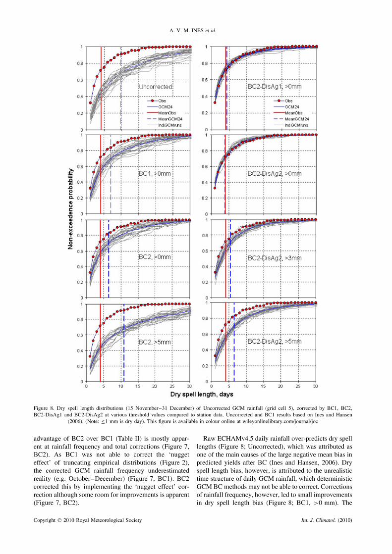
Figure 8. Dry spell length distributions (15 November–31 December) of Uncorrected GCM rainfall (grid cell 5), corrected by BC1, BC2,BC2-DisAg1 and BC2-DisAg2 at various threshold values compared to station data. Uncorrected and BC1 results based on Ines and Hansen

(2006). (Note: ≤1 mm is dry day). This figure is available in colour online at wileyonlinelibrary.com/journal/joc

advantage of BC2 over BC1 (Table II) is mostly appar-ent at rainfall frequency and total corrections (Figure 7,BC2). As BC1 was not able to correct the ‘nuggeteffect’ of truncating empirical distributions (Figure 2),the corrected GCM rainfall frequency underestimatedreality (e.g. October–December) (Figure 7, BC1). BC2corrected this by implementing the ‘nugget effect’ cor-rection although some room for improvements is apparent(Figure 7, BC2).

Raw ECHAMv4.5 daily rainfall over-predicts dry spelllengths (Figure 8; Uncorrected), which was attributed asone of the main causes of the large negative mean bias inpredicted yields after BC (Ines and Hansen, 2006). Dryspell length bias, however, is attributed to the unrealistictime structure of daily GCM rainfall, which deterministicGCM BC methods may not be able to correct. Correctionsof rainfall frequency, however, led to small improvementsin dry spell length bias (Figure 8; BC1, >0 mm). The



updated BC algorithm (BC2) slightly improved the dryspell length distribution compared to BC1 (Figure 8;BC2, >0 mm). Increasing the threshold did not improvedry spell length (Figure 8; BC2, >5 mm).

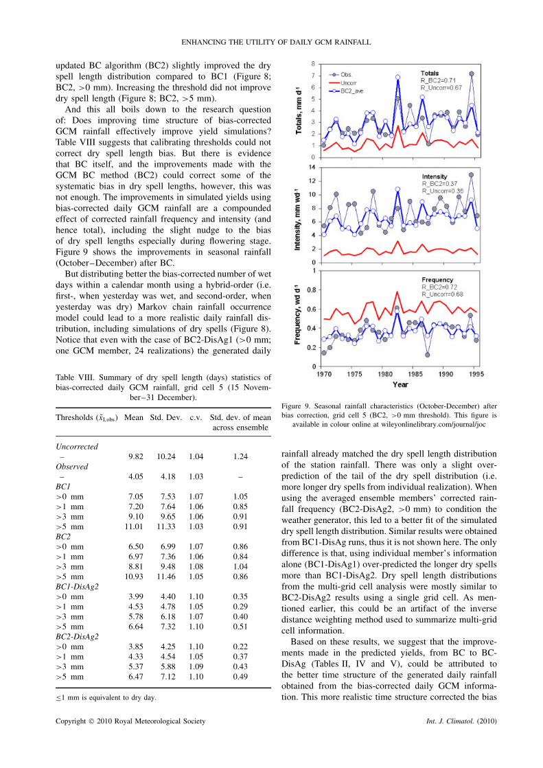
And this all boils down to the research questionof: Does improving time structure of bias-correctedGCM rainfall effectively improve yield simulations?Table VIII suggests that calibrating thresholds could notcorrect dry spell length bias. But there is evidencethat BC itself, and the improvements made with theGCM BC method (BC2) could correct some of thesystematic bias in dry spell lengths, however, this wasnot enough. The improvements in simulated yields usingbias-corrected daily GCM rainfall are a compoundedeffect of corrected rainfall frequency and intensity (andhence total), including the slight nudge to the biasof dry spell lengths especially during flowering stage.Figure 9 shows the improvements in seasonal rainfall(October–December) after BC.

But distributing better the bias-corrected number of wetdays within a calendar month using a hybrid-order (i.e.first-, when yesterday was wet, and second-order, whenyesterday was dry) Markov chain rainfall occurrencemodel could lead to a more realistic daily rainfall dis-tribution, including simulations of dry spells (Figure 8).Notice that even with the case of BC2-DisAg1 (>0 mm;one GCM member, 24 realizations) the generated daily

Table VIII. Summary of dry spell length (days) statistics ofbias-corrected daily GCM rainfall, grid cell 5 (15 Novem-

ber–31 December).

Thresholds (xI,obs) Mean Std. Dev. c.v. Std. dev. of meanacross ensemble

Uncorrected– 9.82 10.24 1.04 1.24

Observed– 4.05 4.18 1.03 –

BC1>0 mm 7.05 7.53 1.07 1.05>1 mm 7.20 7.64 1.06 0.85>3 mm 9.10 9.65 1.06 0.91>5 mm 11.01 11.33 1.03 0.91BC2>0 mm 6.50 6.99 1.07 0.86>1 mm 6.97 7.36 1.06 0.84>3 mm 8.81 9.48 1.08 1.04>5 mm 10.93 11.46 1.05 0.86BC1-DisAg2>0 mm 3.99 4.40 1.10 0.35>1 mm 4.53 4.78 1.05 0.29>3 mm 5.78 6.18 1.07 0.40>5 mm 6.64 7.32 1.10 0.51BC2-DisAg2>0 mm 3.85 4.25 1.10 0.22>1 mm 4.33 4.54 1.05 0.37>3 mm 5.37 5.88 1.09 0.43>5 mm 6.47 7.12 1.10 0.49

≤1 mm is equivalent to dry day.

Figure 9. Seasonal rainfall characteristics (October-December) afterbias correction, grid cell 5 (BC2, >0 mm threshold). This figure is

available in colour online at wileyonlinelibrary.com/journal/joc

rainfall already matched the dry spell length distributionof the station rainfall. There was only a slight over-prediction of the tail of the dry spell distribution (i.e.more longer dry spells from individual realization). Whenusing the averaged ensemble members’ corrected rain-fall frequency (BC2-DisAg2, >0 mm) to condition theweather generator, this led to a better fit of the simulateddry spell length distribution. Similar results were obtainedfrom BC1-DisAg runs, thus it is not shown here. The onlydifference is that, using individual member’s informationalone (BC1-DisAg1) over-predicted the longer dry spellsmore than BC1-DisAg2. Dry spell length distributionsfrom the multi-grid cell analysis were mostly similar toBC2-DisAg2 results using a single grid cell. As men-tioned earlier, this could be an artifact of the inversedistance weighting method used to summarize multi-gridcell information.

Based on these results, we suggest that the improve-ments made in the predicted yields, from BC to BC-DisAg (Tables II, IV and V), could be attributed tothe better time structure of the generated daily rainfallobtained from the bias-corrected daily GCM informa-tion. This more realistic time structure corrected the bias



Figure 10. Sample daily rainfall data, (October-December 1995) before and after bias correction, stochastic disaggregation; grid cell 5. Thisfigure is available in colour online at wileyonlinelibrary.com/journal/joc

in dry spell lengths, thus reducing the mean bias andeliminated most of the systematic errors in the predictedyields (Tables IV and V). Figure 10 shows a sample ofbias corrected daily GCM rainfall (October–December,1995) and how BC-DisAg distributed the number of rain-fall events using the bias-corrected GCM information(>0 mm threshold). Table VIII also shows the dry spelllength statistics with BC-DisAg using various thresholdlevels. Until >1 mm threshold, the corrected mean dryspell length approximates the observed. Beyond that, weobserved a significant deviation but this is more pro-nounced with BC alone (Figure 8, BC-DisAg, higherthresholds).

4. Summary and conclusions

We present a methodology for eliciting useful informationfrom daily GCM rainfall. The BC of daily GCM rainfallcan improve crop yield prediction compared to no cor-rection, although the predicted yields are still negativelybiased. This improvement in yield simulations was asso-ciated with better rainfall frequency, intensity and total ofthe corrected GCM rainfall. However, deterministic BCcannot correct the time structure of daily GCM rainfall,although it was shown that rainfall frequency correctioncould slightly improve dry spell length distributions.

Calibrating thresholds on GCM BC was not successfulto improve the time structure of GCM rainfall. In fact,as we increased the observed threshold value delineatinga wet day, we also decreased the number of wet days,contributing more to longer dry spells in the resultingdaily GCM rainfall. Threshold calibration also tends toshift the rainfall intensity distribution to the right.

Coupling GCM BC with stochastic disaggregation(BC-DisAg) was more successful for simulating betterdry spell length distributions from the corrected dailyGCM rainfall information. Using monthly series of bias-corrected GCM rainfall frequency to adjust transitionprobabilities of the hybrid-order Markov chain rainfalloccurrence model corrected the dry spell length biasadequately. This correction of time structure removedmost of the mean bias error in predicted yields, butnot the spread of the yield distribution. Combiningbias-corrected GCM rainfall frequency and totals forstochastic disaggregation improved both the mean ofpredicted yield distribution and its variance.

Furthermore, the improvements made to the GCMBC method accounting for over- and under-predictionof rainfall frequency, and the ‘nugget effect’ correctionfor truncating empirical distributions, resulted to betterGCM rainfall frequency correction and in the correc-tion of dry spell lengths when coupled with stochasticdisaggregation. We did not get better information fromusing multiple grid cells because the grid cell nearestto the agricultural experimental station dominated thesolutions. Using more robust aggregation methods forsummarizing information better for the multi-grid cellcase (e.g. optimized weighting of grid cell information(not based on distance alone), Model Output Statistics(MOS) correction, etc.) may circumvent the caveat ofdistance-weighted method.

Acknowledgements

This research was supported by NOAA CooperativeGrant Agreement #NA05OAR4311004. We thankMichael Bell and Benno Blumenthal for their help in



the extraction of ECHAMv4.5 daily GCM rainfall fromthe IRI data library. We thank the editor and two anony-mous reviewers for helping us improve the quality of thearticle.

References

Baigorria GA, Jones JW, Shin DW, Mishra A, O’Brien JJ. 2007.Assessing uncertainties in crop model simulations using daily bias-corrected Regional Circulation Model outputs. Climate Research 34:211–222.

Baigorria GA, Jones JW, O’Brien JJ. 2008. Potential predictabilityof crop yield using an ensemble climate forecast by a regionalcirculation model. Agricultural and Forest Meteorology 148:1353–1361.

Baron C, Sultan B, Balme M, Sarr B, Traore S, Lebel T, Janicot S,Dingkuhn M. 2005. From GCM grid cell to agricultural plot:scale issues affecting modelling of climate impact. PhilosophicalTransactions of the Royal Society B 360: 2095–2108.

Challinor AJ, Slingo JM, Wheeler TR, Doblas-Reyes FJ. 2005.Probabilistic simulations of crop yield over western India usingDEMETER seasonal hindcasts ensembles. Tellus A 57: 498–512.

Dobler A, Ahrens B. 2008. Precipitation by a regional climate modeland bias correction in Europe and South Asia. MeteorologischeZeitschrift 17: 499–509.

Elshamy ME, Seierstad IA, Sorteberg A. 2009. Impacts of climatechange on Blue Nile flows using bias-corrected GCM scenarios.Hydrology and Earth System Sciences 13: 551–565.

Goddard L, Mason SJ. 2002. Sensitivity of seasonal climate forecaststo persisted SST anomalies. Climate Dynamics 19: 619–632.

Goddard L, Mason SJ, Zebiak SE, Ropelewski CF, Basher R,Cane MA. 2001. Current approaches to seasonal to interannualclimate predictions. International Journal of Climatology 21:1111–1152.

Hansen JW, Challinor A, Ines AVM, Wheeler T, Moron V. 2006.Translating climate forecasts into agricultural terms: advances andchallenges. Climate Research 33: 27–41.

Hansen JW, Indeje M. 2004. Linking dynamic seasonal climateforecasts with crop simulation for maize yield prediction in semi-aridKenya. Agricultural and Forest Meteorology 125: 143–157.

Hansen JW, Ines AVM. 2005. Stochastic disaggregation of monthlyrainfall data for crop simulation studies. Agricultural and ForestMeteorology 131: 233–246.

Hansen JW, Jones JW. 2000. Scaling-up crop models for climatevariability applications. Agricultural Systems 65: 43–72.

Hansen JW, Mavromatis T. 2001. Correcting low-frequency variabilitybias in stochastic weather generators. Agricultural and ForestMeteorology 109: 297–310.

Indeje M, Semazzi FHM, Ogallo LJ. 2000. ENSO signals in EastAfrican rainfall and their prediction potentials. International Journalof Climatology 20: 19–46.

Ines AVM, Hansen JW. 2006. Bias correction of daily GCM rainfall forcrop simulation studies. Agricultural and Forest Meteorology 138:44–53.

Ines AVM, Hansen JW. 2009. Extracting useful information from dailyGCM rainfall for cropping system modeling. AgSAP Conference2009. Egmond Aan Zee: The Netherlands.

Jones JW, Hoogenboom G, Porter CH, Boote KJ, Batchelor WD,Hunt LA, Wilkens PW, Singh U, Gijsman AJ, Ritchie JT. 2003. TheDSSAT cropping system model. European Journal of Agronomy 18:235–265.

Katz RW, Parlange MB. 1998. Overdispersion phenomenon instochastic modeling of precipitation. Journal of Climate 11:591–601.

Keating BA, Wafula BM, Watiki JM. 1992. Exploring strategies forincreased productivity – the case for maize in semi-arid EasternKenya. In A Search for Strategies for Sustainable DrylandCropping in Semi-arid Eastern Kenya, ACIAR Proceedings , No. 41.Probert ME (ed). Australian Centre for International AgriculturalResearch: Canberra, 90–101.

Mavromatis T, Jones PD. 1999. Evaluation of HADCM2 and direct useof daily GCM data in impact assessment studies. Climatic Change41: 583–614.

Mearns LO, Rosenzweig C, Goldberg R. 1996. The effects of changesin daily and interannual climatic variability on CERES-Wheat: asensitivity study. Climatic Change 32: 257–292.

Mishra A, Hansen JW, Dingkuhn M, Baron C, Traore SB, Ndiaye O,Ward MN. 2008. Sorghum yield prediction from seasonal rainfallforecasts in Burkina Faso. Agricultural and Forest Meteorology 148:1798–1814.

Mishra AK, Singh VP. 2009. Analysis of drought severity-area-frequency curves using a general circulation model and scenariouncertainty. Journal of Geophysical Research D: Atmospheres114(6): D06120.

Mishra AK, Ozger M, Singh VP. 2009. Trend and persistence ofprecipitation under climate change scenarios for Kansabati basin,India. Hydrological Processes 23: 2345–2357.

Riha SJ, Wilks DS, Simeons P. 1996. Impacts of temperature andprecipitation variability on crop model predictions. Climatic Change32: 293–311.

Ritchie JT, Singh U, Godwin DC, Bowen WT. 1998. Cereal growth,development and yield. In Understanding Options for AgriculturalProduction, Tsuji GY, Hoogenboom G, Thornton PK (eds). KluwerAcademic Publishers: Dordrecht, 79–98.

Robertson AW, Ines AVM, Hansen JW. 2007. Downscaling ofseasonal precipitation for crop simulation. Journal of AppliedMeteorology and Climatology 46: 677–693.

Roeckner E, Arpe K, Bengtsson L, Claussen CM, Dumenil L, Esch M,Giorgetta M, Schiese U, Schulzweida U. 1996. The atmosphericgeneral circulation model ECHAM-4: model description andsimulation of present-day climate. Report No. 218, Max PlanckInstitute for Meteorology. Hamburg.

Schmidli J, Frei C, Vidale PL. 2006. Downscaling from GCMprecipitation: a benchmark for dynamical and statistical downscalingmethods. International Journal of Climatology 26: 679–689.

Semenov MA, Doblas-Reyes FJ. 2007. Utility of dynamical seasonalforecasts in predicting crop yield. Climate Research 34: 71–81.

Sharma D, Gupta AD, Babel MS. 2007. Spatial disaggregation of bias-corrected GCM precipitation for improved hydrologic simulation:Ping River Basin, Thailand. Hydrology and Earth System Sciences11: 1373–1390.

Stern RD, Coe R. 1984. A model fitting analysis of daily rainfall data.Journal of Royal Statistical Society A 147: 1–34.

Tsuji GT, Uehara G, Salas S. (eds). 1994. DSSATv3.0, Vol. 3.University of Hawaii: Honolulu, Hawaii, p. 286.

Wilks DS. 1995. Statistical Methods in the Atmospheric Sciences,Academic Press: San Diego.

Wilks DS. 1999. Interannual variability and extreme-value character-istics of several stochastic daily precipitation models. Agriculturaland Forest Meteorology 93: 153–169.

Wilks DS, Wilby RL. 1999. The weather generation game: a reviewof stochastic weather models. Progress in Physical Geography 23:329–357.

Willmott CJ. 1982. Some comments on the evaluation of modelperformance. Bulletin of the American Meteorological Society 63:1309–1313.

Woolhiser DA, Roldan J. 1982. Stochastic daily precipitation models.2. A comparison of distributions of amounts. Water ResourcesResearch 18: 1461–1468.


enhancing the utility of daily gcm rainfall for crop yield

Documents