enhancing resilience of highway bridges through seismic retrofit

Enhancing resilience of highway bridges through seismic retrofit

Ashok Venkittaraman1 and Swagata Banerjee2,*,†

1Technip North America, Houston, TX 77079, USA2Department of Civil and Environmental Engineering, The Pennsylvania State University, University Park, PA 16802, USA

SUMMARY

The present study evaluates seismic resilience of highway bridges that are important components of highwaytransportation systems. To mitigate losses incurred from bridge damage during seismic events, bridge retro-fit strategies are selected such that the retrofit not only enhances bridge seismic performance but also im-proves resilience of the system consisting of these bridges. To obtain results specific to a bridge, areinforced concrete bridge in the Los Angeles region is analyzed. This bridge was severely damaged duringthe Northridge earthquake because of shear failure of one bridge pier. Seismic vulnerability model of thebridge is developed through finite element analysis under a suite of time histories that represent regionalseismic hazard. Obtained bridge vulnerability model is combined with appropriate loss and recovery modelsto calculate seismic resilience of the bridge. Impact of retrofit on seismic resilience is observed by applyingsuitable retrofit strategy to the bridge assuming its undamaged condition prior to the Northridge event. Dif-ference in resilience observed before and after bridge retrofit signified the effectiveness of seismic retrofit.The applied retrofit technique is also found to be cost-effective through a cost-benefit analysis. First ordersecond moment reliability analysis is performed, and a tornado diagram is developed to identify major un-certain input parameters to which seismic resilience is most sensitive. Statistical analysis of resilienceobtained through random sampling of major uncertain input parameters revealed that the uncertain natureof seismic resilience can be characterized with a normal distribution, the standard deviation of which repre-sents the uncertainty in seismic resilience. Copyright © 2013 John Wiley & Sons, Ltd.

Received 12 May 2013; Revised 17 October 2013; Accepted 25 October 2013

KEY WORDS: resilience; highway bridges; seismic fragility; parameter sensitivity; random sampling;benefit-cost analysis

1. INTRODUCTION

A natural disaster is the consequence of an extreme natural hazard such as earthquake, flood, hurricane,tornado, and landslide. It leads to economic, human, and/or environmental losses to a society. Theresulting loss depends on the resistance of the affected population to survive against the disastrousevent, called its resilience. Disaster resilience of a civil infrastructure system is defined in literatureas a function that indicates the capability of the system to sustain a level of functionality over aperiod decided by owners or the society.

Bridges are significant component of highway transportation systems that serve as a key mode ofground transportation and sometimes act as an important feeder system to other modes oftransportation such as railroad systems, port facilities, and air travel. Damage of highway bridgesdue to extreme events may cause severe disruption to the normal functionality of highwaytransportation systems and may further impact on the performance of other modes of transport.Bridge damage not only causes direct economic losses due to postevent bridge repair and restoration

*Correspondence to: Swagata Banerjee, Department of Civil and Environmental Engineering, The Pennsylvania StateUniversity, University Park, PA 16802, USA.†E-mail: [email protected]

Copyright © 2013 John Wiley & Sons, Ltd.

EARTHQUAKE ENGINEERING & STRUCTURAL DYNAMICSEarthquake Engng Struct. Dyn. 2014; 43:1173–1191Published online 26 November 2013 in Wiley Online Library (wileyonlinelibrary.com). DOI: 10.1002/eqe.2392

but also produces indirect losses arising from network downtime, traffic delay, and businessinterruptions. Failure of large numbers of highway bridges in California during the 1971 SanFernando, 1989 Loma Prieta, and 1994 Northridge earthquakes has severely disrupted the normalfunctionality of regional highway transportation systems and caused sudden and undesired changesin technical, organizational, societal, and economic conditions of communities served by thesesystems. Prevention is better than cure—this simple yet powerful adage becomes of profoundimportance when such a disaster condition is thought of. Along this line, ‘recovery’ and ‘resilience’have become key points in dealing with extreme events, if not to prevent completely, but tominimize their negative consequences and to maximize disaster resilience of highway transportationsystems.

Seismic retrofitting of highway bridges is one of the most common approaches undertaken by stateDepartments of Transportation (state DOTs) and bridge owners to enhance system performance ofbridges during seismic events. Types of seismic retrofit strategies applied to a bridge depend onvarious factors including bridge attributes, configurations, accessibility, and demand from seismichazard. Common seismic retrofit techniques for bridges include lateral confinement of bridge piersusing steel or composite jackets, installation of restrainers at abutments and expansion joints,seismic isolation through bearings, and installation of bigger foundations [1–4]. While all thesebridge retrofit techniques may be effective in mitigating seismic risk of bridges, adequacy of theirapplication and effectiveness may greatly depend on enhanced seismic functionality of highwaynetwork because of retrofit, reduction in postearthquake losses, and benefit to cost ratio of bridgeretrofitting. Hence, the basis for selecting bridge retrofit technique should include expected posteventlosses and cost incurred from seismic retrofit in addition to the enhancement in bridge performanceand network functionality. In this relation, calculation of resilience is identified as a meaningful wayto express loss and recovery of system functionality after a natural disaster [5–15]. Seismicresilience of a highway bridge can be represented as an integrated measure of bridge seismicperformance, expected losses, and recovery after the occurrence of seismic events. Therefore,calculation of bridge resilience before and after the application of a retrofit strategy will not onlyindicate the effectiveness of this strategy in improving bridge seismic performance but also exhibitthe impact of retrofit on system functionality under regional seismic hazard.

This present study evaluates effectiveness of retrofit techniques to enhance seismic resilience ofhighway bridges. A reinforced concrete bridge in the La Cienega-Venice Boulevard sector of SantaMonica (I-10) freeway in Los Angeles, California is selected as a test-bed bridge. This freeway runsacross eight states from Florida to the Pacific. In 1993, this freeway was reported to be the world’sbusiest freeway carrying an approximate average daily traffic of 261,000 [16]. During the 1994Northridge earthquake, the test-bed bridge was severely damaged primarily because of shear failureof one of the bridge piers. Postevent reconnaissance indicated that the failure was initiated frominadequate lateral confinement of pre-1971 designed bridge piers. Due to this, vertical load carryingcapacity of the bridge reduced significantly during the seismic event resulting in crushing of coreconcrete and buckling of longitudinal rebars of bridge piers [17]. Seismic vulnerability of thepredamaged bridge is assessed through finite element (FE) analysis of the bridge under a suite oftime histories that represent seismic hazard at the bridge site. Seismic resilience of the as-builtbridge is calculated using appropriate loss and recovery models. To observe the effectiveness ofbridge retrofit in enhancing seismic resilience, bridge piers are retrofitted with steel jackets assumingthe undamaged condition of the bridge prior to the Northridge event. Seismic vulnerability of theretrofitted bridge is estimated to calculate seismic resilience after retrofitting. Difference in seismicresilience before and after retrofit is considered to be a signature representing the adequacy andeffectiveness of applied retrofit technique. Cost-benefit study is performed assuming 30 to 50 yearservice life of the retrofitted bridge to evaluate the cost-effectiveness of applied seismic retrofittechnique.

First order second moment (FOSM) reliability analysis is performed to identify major uncertaininput parameters to which seismic resilience of the original un-retrofitted bridge estimated for theNorthridge earthquake is most sensitive. For this, parameter uncertainties associated with bridgevulnerability analysis and resilience estimation modules are considered. A tornado diagram isdeveloped to further support the observations made from FOSM analysis regarding the hierarchy of

1174 A. VENKITTARAMAN AND S. BANERJEE

Copyright © 2013 John Wiley & Sons, Ltd. Earthquake Engng Struct. Dyn. 2014; 43:1173–1191DOI: 10.1002/eqe

uncertain input parameters. To characterize the uncertain nature of seismic resilience, statisticalanalysis of resilience obtained through random sampling of major uncertain input parameters isperformed. Though seismic hazard is discussed in this paper, the described approach of selecting themost suitable retrofit strategy can be extended to other types of natural hazards and structural type.

2. SEISMIC RESILIENCE

Past studies have defined and calculated resilience of various lifeline systems such as acute carehospitals, water supply systems, power transmission systems, and transportation systems [5–15]. Ingeneral, resilience is defined in these studies as a dimensionless quantity representing the rapidity ofthe system to revive from a damaged condition to the predamaged functionality level. Loss due to anatural event and postevent performance recovery of a system are the two major components toquantify disaster resilience of a civil infrastructure system. For a single seismic event, resilience canbe expressed as [12]

R ¼ ∫t0EþTLC

t0E

Q tð ÞTLC

dt (1)

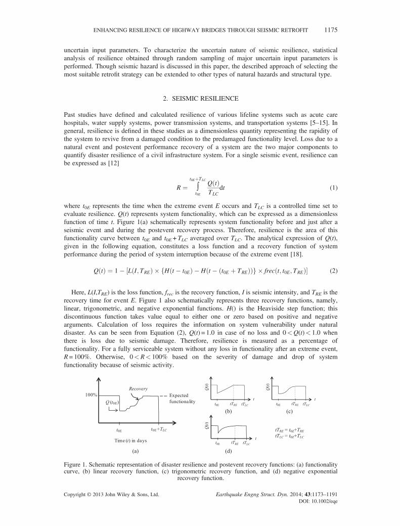
where t0E represents the time when the extreme event E occurs and TLC is a controlled time set toevaluate resilience. Q(t) represents system functionality, which can be expressed as a dimensionlessfunction of time t. Figure 1(a) schematically represents system functionality before and just after aseismic event and during the postevent recovery process. Therefore, resilience is the area of thisfunctionality curve between t0E and t0E + TLC averaged over TLC. The analytical expression of Q(t),given in the following equation, constitutes a loss function and a recovery function of systemperformance during the period of system interruption because of the extreme event [18].

Q tð Þ ¼ 1� L I; TREð Þ � H t � t0Eð Þ � H t � t0E þ TREð Þð Þf g � frec t; t0E; TREð Þ½ � (2)

Here, L(I,TRE) is the loss function, frec is the recovery function, I is seismic intensity, and TRE is therecovery time for event E. Figure 1 also schematically represents three recovery functions, namely,linear, trigonometric, and negative exponential functions. H() is the Heaviside step function; thisdiscontinuous function takes value equal to either one or zero based on positive and negativearguments. Calculation of loss requires the information on system vulnerability under naturaldisaster. As can be seen from Equation (2), Q(t) = 1.0 in case of no loss and 0<Q(t)< 1.0 whenthere is loss due to seismic damage. Therefore, resilience is measured as a percentage offunctionality. For a fully serviceable system without any loss in functionality after an extreme event,R= 100%. Otherwise, 0<R< 100% based on the severity of damage and drop of systemfunctionality because of seismic activity.

Figure 1. Schematic representation of disaster resilience and postevent recovery functions: (a) functionalitycurve, (b) linear recovery function, (c) trigonometric recovery function, and (d) negative exponential

recovery function.

ENHANCING RESILIENCE OF HIGHWAY BRIDGES THROUGH SEISMIC RETROFIT 1175


2.1. Vulnerability of a system or system component

For highway transportation systems, bridges are generally considered as the most seismicallyvulnerable components. The present study measures bridge vulnerability in the form of fragilitycurves. Fragility curves represent the probability of exceeding in a bridge damage state under certainintensity of ground motions such as peak ground acceleration or PGA [19, 20]. Two-parameterlognormal distributions are generally used to develop fragility curves. The analytical expression of afragility curve is given as

F PGAj; ck; ζ k� � ¼ Φ

ln PGAj=ck� �

ζ k

� �(3)

where PGAj represents PGA of a ground motion j and k represents bridge damage states such as minor,moderate, major damage, and complete collapse. The two parameters ck (median value) and ζ k (log-standard deviation) are fragility parameters for a damage state k. These parameters can be estimatedby maximizing the likelihood function L given as follows.

L ¼ ∏j

F PGAj; ck; ζ k� �� rj 1� F PGAj; ck; ζ k

� �� 1�rj (4)

Here, rj= 0 or 1 depending on whether or not the bridge sustains the damage state k under the jth

ground motion. Other intensity measures such as peak ground velocity, spectral acceleration,spectral velocity, and spectral intensity can also be used to represent seismic intensity. However, theuse of any of the above intensity measures in the development of seismic fragility curves providesno additional advantage over the use of PGA [21].

2.2. Loss function

The loss function incorporates all direct and indirect losses from a postevent degraded system over theperiod of system restoration. The direct loss for a bridge seismic damage arises because of bridgerestoration after the seismic event. It includes the cost associated with postevent repair andrehabilitation of damaged bridges or bridge components. Hence, direct loss due to a seismic eventcan be calculated by multiplying the occurrence probability of the event and failure probability of asystem (or system component) under this event [22, 23]. For a bridge, direct economic loss (CrE)resulted from an event E can be evaluated in terms of a dimensionless cost term LD that representsthe ratio of restoration cost CrE to replacement cost C as

LD ¼ CrE

C¼ ∑

kPE DS ¼ kð Þ � rk (5)

where k represents the damage states of the bridge, PE (DS = k) is the probability of bridge failure atdamage state k during the seismic event E, and rk is the damage ratio corresponding to damage statek. Values of PE (DS = k) and rk can be obtained, respectively, from bridge fragility curves developedfor various damage states and HAZUS [24]. Replacement cost C can be evaluated by multiplyingbridge deck area with the unit area replacement cost [22].

Indirect loss (LID) arises because of the disrupted functionality of the system after an event. Forhighway transportation systems, indirect losses consist of rental, relocation, business interruptions,traffic delay, loss of opportunity, losses in revenue, and so on. In addition, casualty losses may alsobe included in the indirect loss model to calculate resilience of critical care facilities such ashospitals [12]. Indirect losses are time dependent. These losses are maximum immediately after theextreme event and gradually reduce as bridge restoration takes place. Past studies on highwaybridges have taken indirect loss to be 5–20 times greater than the direct loss [25]. More specificvalue of indirect to direct loss ratio can be calculated if information on traffic flow in a highwaynetwork before and after an earthquake can be obtained and dynamic equilibrium using network



capacity and traffic demand can be established [22]. Such as comprehensive traffic analysis is beyondthe scope of the present study. Hence, an expected value for indirect to direct loss ratio of 13 isassumed in this study for each bridge damage state. A similar approach has been adopted inDenneman [25]. A sensitivity study presented later in this paper investigated the impact of this ratioon seismic resilience.

2.3. Recovery function

The recovery function (frec) describes a path following that postevent restoration of bridges is expectedto take place. Development of an appropriate mathematical model for the recovery function involvesextreme difficulty because of the dependence of postevent bridge recovery process on several factorsincluding the availability of fund. Cimellaro [15] suggested the generation of empirical or analyticalrecovery functions based on real-life data or on the type of analysis. For analytical recoveryfunctions, five different recovery functions are proposed that are further grouped under short-termand long-term recovery models. Among these, the long-term recovery models are of interest here asthe present study includes the postevent recovery phase within the framework of resilienceestimation. Long-term recovery models included linear, negative exponential, and trigonometricrecovery functions. A linear postevent bridge recovery process with a probabilistic distribution ofpostevent recovery time is also proposed by Zhou et al. [22] on the basis of bridge recoveryprocesses observed in real-time after severe earthquakes in past. These previous studies used samerecovery pattern (i.e., either linear or trigonometric or exponential) irrespective of seismic damagestates of structural components. Decò et al. [14] proposed to use different recovery patterns fordifferent seismic damage states of bridges because bridges with different seismic damage states mayhave different levels of accessibility after the seismic event. A variety of postevent bridge restorationpatterns (such as positive and negative exponential and stepwise) are assigned to different bridgedamage states on the basis of subjective judgments.

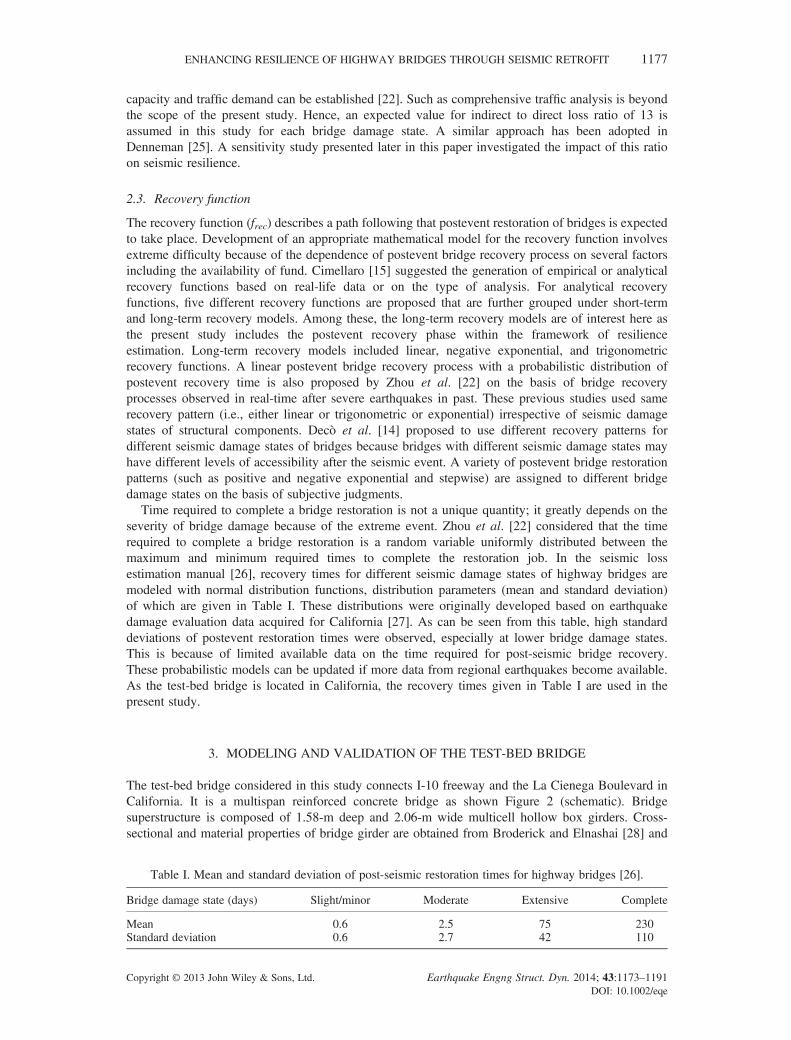
Time required to complete a bridge restoration is not a unique quantity; it greatly depends on theseverity of bridge damage because of the extreme event. Zhou et al. [22] considered that the timerequired to complete a bridge restoration is a random variable uniformly distributed between themaximum and minimum required times to complete the restoration job. In the seismic lossestimation manual [26], recovery times for different seismic damage states of highway bridges aremodeled with normal distribution functions, distribution parameters (mean and standard deviation)of which are given in Table I. These distributions were originally developed based on earthquakedamage evaluation data acquired for California [27]. As can be seen from this table, high standarddeviations of postevent restoration times were observed, especially at lower bridge damage states.This is because of limited available data on the time required for post-seismic bridge recovery.These probabilistic models can be updated if more data from regional earthquakes become available.As the test-bed bridge is located in California, the recovery times given in Table I are used in thepresent study.

3. MODELING AND VALIDATION OF THE TEST-BED BRIDGE

The test-bed bridge considered in this study connects I-10 freeway and the La Cienega Boulevard inCalifornia. It is a multispan reinforced concrete bridge as shown Figure 2 (schematic). Bridgesuperstructure is composed of 1.58-m deep and 2.06-m wide multicell hollow box girders. Cross-sectional and material properties of bridge girder are obtained from Broderick and Elnashai [28] and

Table I. Mean and standard deviation of post-seismic restoration times for highway bridges [26].

Bridge damage state (days) Slight/minor Moderate Extensive Complete

Mean 0.6 2.5 75 230Standard deviation 0.6 2.7 42 110



Lee and Elnashai [29]. The bridge is supported on six 1.219-m diameter circular piers at four bentlocations. Bent 5 is a multicolumn bent with three identical piers. Bents 6 to 8 each has single pierwith the same diameter as of the piers in bent 5. Based on reinforcement used, these piers haveeither type ‘H’ (in bent 5) or type ‘M’ (in bents 6 to 8) cross sections (Figure 2). Bent 9 has arectangular wall section. All pier–girder connections are monolithic. Specific properties of thesebents are discussed later in this paper. The bridge has an in-span expansion joint just after bent 6.

Broderick and Elnashai [28] analyzed the nonlinear response of the bridge under the Northridgeearthquake ground motions and made a qualitative comparison between analytical bridge responsewith that observed during the earthquake. As the bridge was a part of freeway system, it wasdifficult to numerically simulate the accurate boundary condition of the bridge. Broderick andElnashai [28] developed four FE bridge models by changing boundary conditions. Effectiveness ofthese four models was judged by comparing the numerical response of the bridge with that observedduring the Northridge earthquake. This comparison showed that the consideration of fixed boundaryon freeway side (west side) and hinged boundary (i.e., moment release) on the east side of thebridge provided the closest match between numerical and observed bridge response. Thus, thecomparison helped in establishing a realistic numerical model for the bridge. To pursue the presentstudy, results presented in Broderick and Elnashai [28] are used as baseline to validate the FE modelof the bridge developed as a part of the present study. Consistency is maintained in assigningboundary conditions and material properties of various bridge components for model valuation(Figure 2).

3.1. Modeling of bridge components

Finite element model of the bridge is developed using SAP2000 [30]. Modeling of various bridgecomponents and their geometric and material properties are discussed next.

3.1.1. Bridge girder. A 140.4-m long bridge girder is modeled using linear elastic beam–columnelements as this component of the bridge is expected to respond within the elastic range duringseismic excitation. These beam–column elements are aligned along the center line of the bridgedeck. To obtain properties of beam–column elements, cross section of bridge girder is modeled inSTAAD [31], and obtained properties are used in SAP2000 as input.

3.1.2. Bridge piers. During seismic excitation, the maximum bending moment generates at pier ends.This often leads to the formation of plastic hinges at these locations when the generated momentexceeds the plastic moment capacity of these sections. To model such nonlinear behavior at bridgepier ends, nonlinear rotational springs are introduced in bridge models at the top and bottom of each

Figure 2. (a) The test-bed bridge (schematic), (b) cross-section of bridge girder, and (c) cross sections of type‘H’ and ‘M’ piers (all units are in mm).



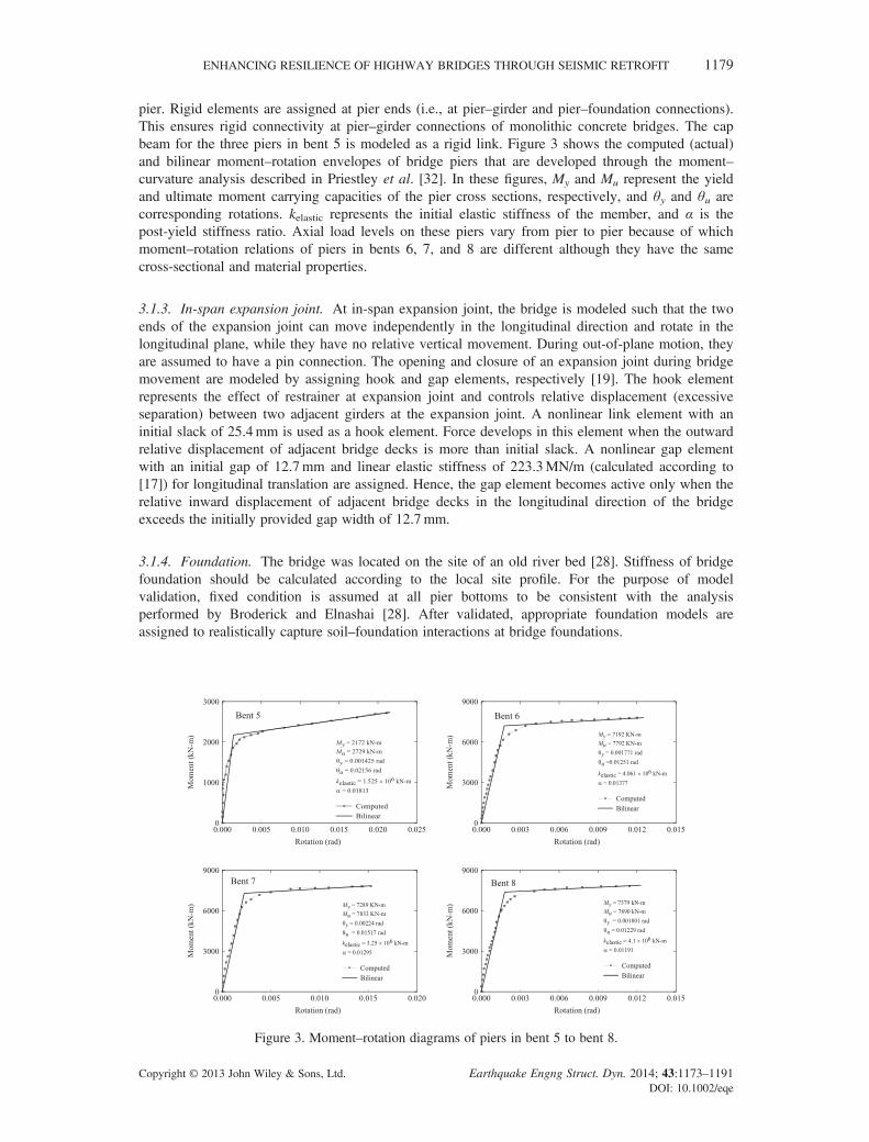
pier. Rigid elements are assigned at pier ends (i.e., at pier–girder and pier–foundation connections).This ensures rigid connectivity at pier–girder connections of monolithic concrete bridges. The capbeam for the three piers in bent 5 is modeled as a rigid link. Figure 3 shows the computed (actual)and bilinear moment–rotation envelopes of bridge piers that are developed through the moment–curvature analysis described in Priestley et al. [32]. In these figures, My and Mu represent the yieldand ultimate moment carrying capacities of the pier cross sections, respectively, and θy and θu arecorresponding rotations. kelastic represents the initial elastic stiffness of the member, and α is thepost-yield stiffness ratio. Axial load levels on these piers vary from pier to pier because of whichmoment–rotation relations of piers in bents 6, 7, and 8 are different although they have the samecross-sectional and material properties.

3.1.3. In-span expansion joint. At in-span expansion joint, the bridge is modeled such that the twoends of the expansion joint can move independently in the longitudinal direction and rotate in thelongitudinal plane, while they have no relative vertical movement. During out-of-plane motion, theyare assumed to have a pin connection. The opening and closure of an expansion joint during bridgemovement are modeled by assigning hook and gap elements, respectively [19]. The hook elementrepresents the effect of restrainer at expansion joint and controls relative displacement (excessiveseparation) between two adjacent girders at the expansion joint. A nonlinear link element with aninitial slack of 25.4mm is used as a hook element. Force develops in this element when the outwardrelative displacement of adjacent bridge decks is more than initial slack. A nonlinear gap elementwith an initial gap of 12.7mm and linear elastic stiffness of 223.3MN/m (calculated according to[17]) for longitudinal translation are assigned. Hence, the gap element becomes active only when therelative inward displacement of adjacent bridge decks in the longitudinal direction of the bridgeexceeds the initially provided gap width of 12.7mm.

3.1.4. Foundation. The bridge was located on the site of an old river bed [28]. Stiffness of bridgefoundation should be calculated according to the local site profile. For the purpose of modelvalidation, fixed condition is assumed at all pier bottoms to be consistent with the analysisperformed by Broderick and Elnashai [28]. After validated, appropriate foundation models areassigned to realistically capture soil–foundation interactions at bridge foundations.

Figure 3. Moment–rotation diagrams of piers in bent 5 to bent 8.



3.2. Northridge earthquake ground motions records

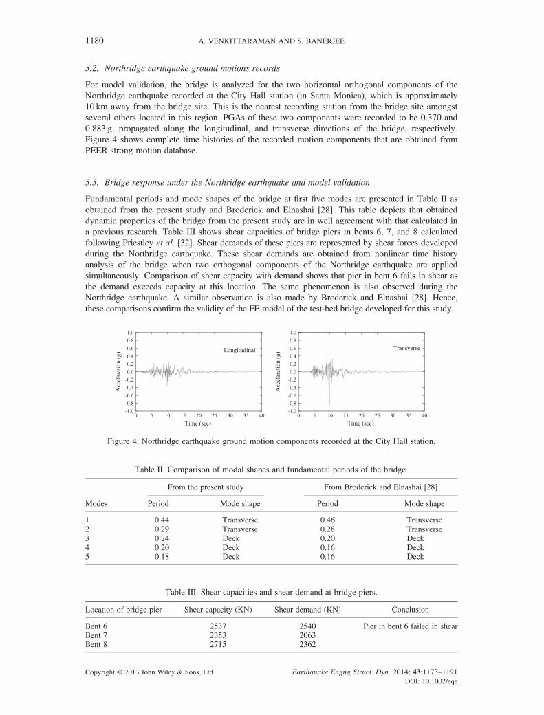
For model validation, the bridge is analyzed for the two horizontal orthogonal components of theNorthridge earthquake recorded at the City Hall station (in Santa Monica), which is approximately10 km away from the bridge site. This is the nearest recording station from the bridge site amongstseveral others located in this region. PGAs of these two components were recorded to be 0.370 and0.883 g, propagated along the longitudinal, and transverse directions of the bridge, respectively.Figure 4 shows complete time histories of the recorded motion components that are obtained fromPEER strong motion database.

3.3. Bridge response under the Northridge earthquake and model validation

Fundamental periods and mode shapes of the bridge at first five modes are presented in Table II asobtained from the present study and Broderick and Elnashai [28]. This table depicts that obtaineddynamic properties of the bridge from the present study are in well agreement with that calculated ina previous research. Table III shows shear capacities of bridge piers in bents 6, 7, and 8 calculatedfollowing Priestley et al. [32]. Shear demands of these piers are represented by shear forces developedduring the Northridge earthquake. These shear demands are obtained from nonlinear time historyanalysis of the bridge when two orthogonal components of the Northridge earthquake are appliedsimultaneously. Comparison of shear capacity with demand shows that pier in bent 6 fails in shear asthe demand exceeds capacity at this location. The same phenomenon is also observed during theNorthridge earthquake. A similar observation is also made by Broderick and Elnashai [28]. Hence,these comparisons confirm the validity of the FE model of the test-bed bridge developed for this study.

Figure 4. Northridge earthquake ground motion components recorded at the City Hall station.

Table II. Comparison of modal shapes and fundamental periods of the bridge.

Modes

From the present study From Broderick and Elnashai [28]

Period Mode shape Period Mode shape

1 0.44 Transverse 0.46 Transverse2 0.29 Transverse 0.28 Transverse3 0.24 Deck 0.20 Deck4 0.20 Deck 0.16 Deck5 0.18 Deck 0.16 Deck

Table III. Shear capacities and shear demand at bridge piers.

Location of bridge pier Shear capacity (KN) Shear demand (KN) Conclusion

Bent 6 2537 2540 Pier in bent 6 failed in shearBent 7 2353 2063Bent 8 2715 2362



4. SEISMIC RESILIENCE OF THE BRIDGE

Broderick and Elnashai [28] used fixed conditions at bridge pier bases. The same condition isconsidered in the initial FE model of the test-bed bridge for the validation purpose. Post-validation,boundary conditions at pier bases are revised to include the effect of foundation–soil interaction ondynamic response of the bridge. From literature, it is found that type ‘M’ and ‘H’ piers of the bridgewere supported on groups of 14 and 12 piles, respectively [28]. Each pile had 0.4m diameter.Consequently, translational foundation springs are assigned at pier bottoms in the longitudinal andtransverse directions of the bridge. Spring constants in lateral direction are calculated considering7 kN/mm lateral stiffness of each pile [33, 34]. Thus, lateral foundation stiffness for type ‘M’ and‘H’ piles is calculated to be 98 and 84 kN/mm, respectively. Foundation joints are restrained in thevertical direction, and rotational degrees of freedom at these joints about all directions are constrained.

4.1. Bridge fragility curves

To develop fragility curves, time history analyses of the bridge are performed under 60 ground motionsthat were originally generated by the Federal Emergency Management Agency for the Los Angelesregion in California.1 These ground motions include both recorded and synthetic motions and arecategorized into three sets having annual exceedance probabilities of 2%, 10%, and 50% in 50 years.Each set has 20 ground motions. The wide range of seismic hazard covered through these motions ispreferable for seismic fragility analysis of the bridge.

During the Northridge earthquake, a major horizontal ground motion component propagated alongthe transverse direction of the bridge resulting in shear failure of pier in bent 6 in this direction. Hence,the test-bed bridge is most vulnerable in the transverse direction. To be consistent with the actualdamage of the bridge, seismic fragility analysis is performed by applying ground motions in thetransverse direction of the bridge. Bridge seismic damage is characterized through shear and flexuralfailures of bridge piers. These two failure modes are assumed to govern the global failure of thebridge. Other possible seismic bridge failure modes such as unseating of bridge girders and failureat expansion joint are assumed to be non-governing failure modes. In general, shear failure of abridge pier is brittle in nature and sometimes causes irreversible damage to bridges. Hence, such amode of failure is considered here as an ultimate damage (i.e., complete collapse) of the bridge. Forflexural damage of bridge piers, HAZUS [24] provided five different bridge damage states namelyno, minor (or slight), moderate, major (or extensive) damage, and complete collapse. Among these,the complete collapse state is the ultimate damage state of the bridge, and others are namedaccording to the severity of bridge seismic damage without complete collapse.

To generate fragility curves of the bridge, shear and flexural damage of the bridge are defined in aquantitative manner. Seismic damage states are ranked with k= 1 to 4 in which k = 1 represents minordamage and k = 4 represents complete collapse. If shear failure occurs because of the jth ground motion,the bridge is considered to have damage condition rj= 1 at damage state k = 4 (Equation (4)). Forflexural damage, bridge damage condition (rj= 0 or 1) at a particular damage state is defined on thebasis of rotational ductility of bridge piers. By definition, rotational ductility (μθ) is the ratio ofrotation (θ) of bridge piers to the yield rotation (θy) measured at the same location. Thus, rotationalductility of all piers at yield is equal to 1.0 (=θy /θy), whereas the same for the ultimate state (=θu /θy; θuis ultimate rotation of bridge piers, Figure 3) will vary from pier to pier. During time historyanalyses of the bridge under 60 motions, rotational time histories are recorded at both top andbottom of all bridge piers where plastic hinges are likely to appear. Rotational ductility for eachpier is obtained by dividing maximum rotations from rotational time histories with yield rotationsof corresponding locations that are obtainable from moment–rotation plots shown in Figure 3. Theserotational ductility values are considered as a signature representing the flexural response of thebridge under seismic motions.

To define damage condition of the bridge at each damage state due to flexure under 60 groundmotions, rational ductility values are compared with threshold limits. These threshold limits for each

1http://nisee.berkeley.edu/data/strong_motion/sacsteel/ground_motions.html



http://nisee.berkeley.edu/data/strong_motion/sacsteel/ground_motions.html

bridge damage state are shown in Table IV. The bridge was constructed in 1964, so it is reasonable toassume that bridge piers were not properly designed to carry lateral loading from seismic events. Thedeficiency of lateral confinement in bridge piers was also evident from the post-Northridgereconnaissance report [17]. Due to this reason, threshold limits of rotational ductility for variousseismic damage states of the bridge are calculated on the basis of drift limits of non-seismicallydesigned bridge piers recommended in HAZUS [24]. Table IV shows the non-seismic drift limitratios obtained from HAZUS [24] for bridge seismic damage state and corresponding thresholdrotational ductilities of piers in bents 6, 7, and 8. Note that rotational ductility values of the bridge atno damage and complete collapse state are taken to be equal to the yield and ultimate rotationalductility of bridge piers, respectively. As threshold rotational ductility at ultimate state varies forpier to pier, the threshold values for intermediate damage states (i.e., minor, moderate, and major)also vary accordingly. Piers in bent 5 are excluded from this table. Piers in this multicolumn benthave low probability of forming plastic hinges compared to other single-column bents of the bridge.Also, shear forces developed in piers of bent 5 were low relative to their shear capacities. Hence,bent 5 is excluded from shear comparisons as well.

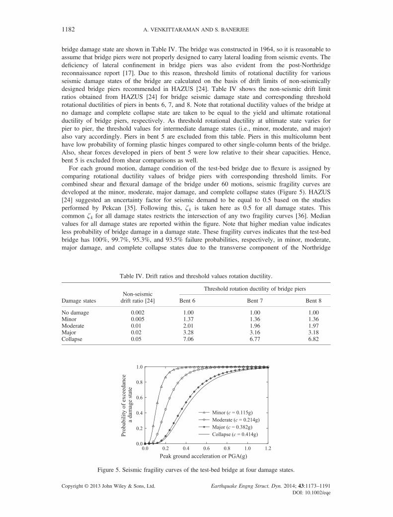
For each ground motion, damage condition of the test-bed bridge due to flexure is assigned bycomparing rotational ductility values of bridge piers with corresponding threshold limits. Forcombined shear and flexural damage of the bridge under 60 motions, seismic fragility curves aredeveloped at the minor, moderate, major damage, and complete collapse states (Figure 5). HAZUS[24] suggested an uncertainty factor for seismic demand to be equal to 0.5 based on the studiesperformed by Pekcan [35]. Following this, ζ k is taken here as 0.5 for all damage states. Thiscommon ζ k for all damage states restricts the intersection of any two fragility curves [36]. Medianvalues for all damage states are reported within the figure. Note that higher median value indicatesless probability of bridge damage in a damage state. These fragility curves indicates that the test-bedbridge has 100%, 99.7%, 95.3%, and 93.5% failure probabilities, respectively, in minor, moderate,major damage, and complete collapse states due to the transverse component of the Northridge

Table IV. Drift ratios and threshold values rotation ductility.

Damage statesNon-seismicdrift ratio [24]

Threshold rotation ductility of bridge piers

Bent 6 Bent 7 Bent 8

No damage 0.002 1.00 1.00 1.00Minor 0.005 1.37 1.36 1.36Moderate 0.01 2.01 1.96 1.97Major 0.02 3.28 3.16 3.18Collapse 0.05 7.06 6.77 6.82

Figure 5. Seismic fragility curves of the test-bed bridge at four damage states.



earthquake (with PGA of 0.883 g). These high probabilities of failure indicate extensive damage of thebridge because of the Northridge earthquake. Thus, the fragility curves can appropriately simulate theseismic vulnerability of the bridge.

4.2. Direct and indirect losses due to the Northridge earthquake

The direct loss due to bridge damage during the Northridge earthquake is calculated followingEquation (5). Damage ratios (rk) at minor, moderate, major, and complete collapse states of thebridge are, respectively, 0.03, 0.08, 0.25, and 2/span number [24]. An overall cost ratio of 0.96 isobtained because of direct and indirect losses from the Northridge earthquake. A sensitivity study isperformed the toward end of this paper by taking various ratios of indirect to direct losses.

4.3. Postevent seismic recovery

To observe the influence of different recovery models on seismic resilience of the bridge, three recoverymodels, linear, negative exponential, and trigonometric [12, 15], are used in this study in the absence ofany precise, case-specific, and real-data-based recovery model for highway bridges. Table I provides thetime required for complete recovery TRE at various seismic damage states of the bridge.

4.4. Seismic resilience

Seismic resilience of the bridge due to the Northridge earthquake is calculated using Equations (1) and(2). Information on bridge seismic vulnerability as obtained from fragility curves (Figure 5) iscombined with postevent loss and recovery functions. Percentage values of bridge seismic resilienceare calculated to be 57.47%, 99.92%, and 57.69%, respectively, when linear, negative exponential,and trigonometric recovery functions are considered. According to these values, linear andtrigonometric recovery models result in approximately the same resilience of the bridge, whereas thenegative exponential recovery function results in very high resilience of the test-bed bridge even ifthe bridge experienced severe damage. This is because of the exponential nature of this recoveryfunction that indicates a very quick post-disaster recovery of a system resulting in minimal loss evenfor a severe damage condition. In reality, the rate of initial recovery is not extremely fast as anexponential function because of postevent reconnaissance, damage assessment, and planning toinitiate rehabilitation before which the recovery process cannot be started. Hence, a negativeexponential recovery model for all bridge damage states is far from reality and not applicable formost of the real-life disaster scenarios. Zhou et al. [22] proposed a linear recovery function on thebasis of experience gained from bridge recovery during past earthquakes. Therefore, the presentstudy uses linear recovery function for the rest part of this paper.

5. BRIDGE SEISMIC RETROFIT AND ENHANCEMENT IN RESILIENCE

To calculate the effectiveness of bridge retrofit in enhancing seismic resilience, retrofit strategies areapplied considering the pre-Northridge undamaged condition of the bridge. The as-built bridgefailed in shear. Hence, bridge retrofit techniques that can facilitate the reduction of shear demand inbridge piers should be selected. After exploring various seismic retrofit possibilities for the test-bedbridge, it is found that the application of steel jackets around bridge piers in bents 6, 7, and 8 is themost effective technique for the current purpose [37]. Seismic vulnerability and resilience of theretrofitted bridge are discussed in this section.

5.1. Moment–rotation behavior of retrofitted bridge piers

Steel jackets have been used as a retrofit measure to enhance the flexural ductility and shear strength ofreinforced concrete bridge piers. These are typically steel casings that are applied to bridge pierskeeping a space of about 50.8mm at pier ends to prevent the jacket from bearing on adjacentmembers. Full length of bridge piers in bents 6, 7, and 8 are jacketed with 0.4mm thick steeljackets. The jacket thickness is decided on the basis of practical consideration of handling the jacket



during retrofit operation. Due to jacketing, moment–rotation behaviors of retrofitted piers are improved(shown in Figure 6) that resulted in enhanced rotational ductility of bridge piers.

5.2. Bridge vulnerability and seismic resilience

Flexural capacity of piers increased significantly after retrofit with steel jackets (Figure 6). Shearcapacity of these piers is estimated following FHWA recommendations [38]. To develop seismicvulnerability model of the retrofitted bridge, time history analysis of the bridge is performed underthe same set of 60 ground motions. It is observed that among 60 cases, only for eight cases thebridge had minor damage due to flexure. No higher flexural damage (such as moderate, major, andcomplete collapse) is observed because bridge excitation under 60 ground motions. Also, no sheardamage is observed in any of the retrofitted bridge piers. To confirm the observation, anothermethod proposed by Sakino and Sun [39] to calculate shear capacity of jacketed concrete bridgepiers is used, and high values of shear capacity of bridge piers are obtained [37]. Based on thisdamage scenario, fragility curve of the retrofitted bridge is developed only at the minor damage state(Figure 7). The median value of the fragility curve is estimated to be 1.27 g with a log-standarddeviation of 0.5.

Figure 6. Moment–rotation diagrams of retrofitted piers in bents 6, 7, and 8.

Figure 7. Fragility curves at minor damage state of the retrofitted bridge.



Due to the strong seismic fragility characteristics of the retrofitted bridge, an overall loss ratio of0.09 is calculated for this bridge under the Northridge earthquake. A linear recovery function withan appropriate model for recovery time is considered to calculate seismic resilience. Result shows99.97% resilience of the bridge under the Northridge earthquake if the bridge were retrofitted withsteel jacket prior to the event. Hence, a 74% increase in seismic resilience of the bridge is observedbecause of seismic retrofitting.

6. SENSITIVITY STUDY AND UNCERTAINTY ANALYSIS

It is recognized that the uncertainties involved with various parameters in the resilience calculationmodulemay introduce uncertainty in the calculated resilience. A sensitivity study is performed to analyze theimpact of various uncertain parameters on seismic resilience. For this, the Northridge earthquake isconsidered as the scenario event for which bridge resilience is estimated. As retrofitting resulted in veryhigh resilience under this scenario event, it would not be possible to distinguish any positive impact ofuncertain parameters on seismic resilience if the sensitivity study is performed on the retrofitted bridge.Thus, the un-retrofitted (original) bridge is used for the sensitivity analysis. Although the original bridgeis too vulnerable under the Northridge earthquake, estimated resilience of the bridge is 57.47% when alinear recovery function is used. This value is the most expected value of resilience when mean valuesof all input parameters are considered. Due to uncertainty in input parameters, a distribution ofresilience will be observed on both sides of the most expected value of resilience. Note that theobservation made from this sensitivity study will be restricted to the case study performed here andmay not be applicable to any bridge and seismic event in general.

6.1. Uncertain parameters

The study considers recovery time, control time, indirect to direct loss ratio, and bridge fragilityparameters (median values) to be the uncertain parameters. These parameters are statisticallyindependent. Other parameters in the analysis module are considered to be deterministic, and theirvalues are kept fixed. For sensitivity study, each uncertain parameter is varied individually whilekeeping all other parameters at their respective mean values. A linear recovery function is used tocalculate resilience for each case.

(1) Recovery time: To observe the sensitivity of seismic resilience to recovery time, TRE at differentbridge damage states are considered to have normal distributions (Table I). The as-built bridgehad shear failure during the Northridge earthquake. Consequently, a normal distribution with amean value of 75 days and standard deviation of 42 days is used to model the uncertainty ofrecovery function for the as-built bridge. Seismic resilience of the bridge is calculated formean ± standard deviation of the recovery time.

(2) Control time: In general, the control time TLC is decided by engineers or bridge owners. It de-pends on the time window of interest, and thus, it can be higher or less than the recovery time.The resilience of the as-built bridge is calculated for mean ± standard deviation of the controltime to calculate its influence on bridge resilience. In the present study, the control time is as-sumed to have a normal distribution with a mean value and standard deviation of 85 days and40 days, respectively.

(3) Indirect to direct loss ratio: The indirect to direct loss ratio may vary between 5 and 20 [25].Even higher variation can be observed on the basis of important physical and decision-making parameters including system redundancy, population type and density, preparednessfor postevent recovery, and fund allocation. The present study considers the most expected valueof indirect to direct loss ratio to be 13 with a standard deviation of 8. With this, the entire rangeof indirect to direct loss ratio as stated in [25] is covered.

(4) Fragility parameters: Fragility parameters of the bridge may vary because of uncertainty of pa-rameters pertaining to the structure and ground motions. A detail uncertainty analysis consider-ing all uncertain bridge and ground motion parameters is beyond the scope of the present study.For this reason, variability (or uncertainty) of fragility curves is quantified in terms of 90%



confidence intervals (between 5% and 95% confidence levels) of these curves. This is a reason-able approach to model the uncertainty associated with fragility curves in absence of any detailuncertainty quantification analysis. Fragility parameters at 95% and 5% confidence levels(with 95% and 5% exceedance probabilities, respectively) are estimated following the proceduredescribed in previous studies [20, 40]. Fragility parameters with 95%, 50%, and 5% confidencebands are listed given in Table V.

6.2. Methods for sensitivity analysis

The FOSM reliability analysis is performed for this sensitivity study. In this, the resilience of the as-built bridge is considered to be the performance function. The value of resilience is calculated formean ± standard deviation of each uncertain parameter. When one parameter is varied, values ofother uncertain parameters are kept at their respective mean values. The analysis provides relativevariances that can be defined as the ratio of variance of resilience due to ith random variable to thetotal variance of resilience due to all random variables [41]. In other words, relative variancerepresents the relative contribution of each uncertain parameter to the total uncertainty of resilience.Hence, values of relative variance indicate the influence of each random variable on the performancefunction. Figure 8 shows the relative variance for each uncertain parameter. As the figure shows, therecovery time TRE and control time TLC have the major influence on seismic resilience of the bridge.Uncertainties in indirect to direct loss ratio and bridge fragility have no influence on resilience.

A tornado diagram, shown in Figure 9, is also developed to represent the hierarchy of uncertainparameters for seismic resilience of the bridge [23]. The center dotted line in the diagram representsthe most expected value of resilience (equal to 57.47%) when mean values of all uncertainparameters are considered. Swings of resilience on both sides of the dotted line show variations ofseismic resilience for mean ± standard deviation values of each uncertain parameter. The longer theswing, the higher the influence of the corresponding input parameter on the output. Again, eachparameter is varied independently keeping all other parameters at their respective mean values. This

Table V. Fragility parameters with 90% confidence intervals.

Damage state

Median fragility parameter (g)

95% confidence 50% confidence 5% confidence

Minor 0.101 0.115 0.130Moderate 0.197 0.214 0.234Major 0.356 0.382 0.407Collapse 0.389 0.414 0.441

Figure 8. Relative variance of uncertain parameters.



tornado diagram shows the same hierarchy as seen from FOSM, and hence confirms the sensitivity ofseismic resilience on recovery time and control time.

6.3. Uncertainty of seismic resilience

It is evident from Figure 9 that seismic resilience is directly proportional to TLC and inverselyproportional to TRE. Figure 10 shows independent influences of TRE and TLC on the variation ofseismic resilience R. In this figure, the variation of R with TLC is obtained when TRE is kept at itsmean value (=75 days). Similarly, TLC is set to its mean value (=85 days) when the variation ofR with TRE is obtained. As the figure shows, resilience varies linearly with TRE and TLC untilTRE =TLC (points A and B on the figure). Beyond this, resilience has nonlinear variations with theseparameters. The linear trend is obvious as a linear recovery function is used to evaluate resiliencefor the sensitivity study. The value of resilience will eventually reaches to an asymptotic value ifTLC and TRE are increased further beyond their maximum values shown in the figure.

To observe the uncertainty in seismic resilience of the bridge under the Northridge earthquake, LatinHypercube random sampling technique [42] is used to generate random combinations of TRE and TLC.The advantage of this sampling technique is the randomness in data selection such that not a single datais repeated to form combinations. Normal distributions of TRE and TLC as discussed in Section 6.1 areused for random sampling. Range of each random variable is divided into four equally probable intervalsthat resulted into 24 random combinations of TRE and TLC. For each combination, seismic resilience isestimated, which is observed to have a wide range variation from 17% to 99%. To estimate theuncertainty associated with these resilience values, a suitable random distribution is assigned to describethe statistical nature of seismic resilience. A goodness-of-fit test revealed that a normal distributioncannot be rejected at significance levels of 0.10 and 0.20 to define seismic resilience. The mean,standard deviation, and coefficient of variation of the normal distribution are 53.73%, 23.98%, and 45%,respectively. This high uncertainty in seismic resilience is the result of high variations considered in

Figure 9. Tornado diagram with uncertain parameters.

Figure 10. Variation of resilience with recovery time TRE and control time TLC.



recovery and control times. The distribution is further verified by plotting resilience values in a normalprobability paper (Figure 11(a)). Figure 11(b) shows the cumulative distribution function (CDF) of thenormal distribution and 24 values of resilience generated through random sampling of TRE and TLC. Asthe figure shows, the generated 24 values of resilience cover 92% probability (between 4th and 96thpercentile values) that is nearly equal to the mean ±2 times standard deviation of the normal CDF.

Note that the quantification of uncertainty of seismic resilience due to uncertain TRE and TLC is thefocus of this section. It is realized that very low value of TLC compared to TRE may not be practicallypossible, and hence all values of resilience as obtained through the random sampling of TRE and TLCmay not be realistic to the test-bed bridge. However, all combinations of TRE and TLC are consideredin the study for the completeness of uncertainty analysis. Furthermore, the nature of obtaineddistribution of resilience and distribution parameters may change if different distributions of TRE andTLC are considered. Hence, the quantified uncertainty in seismic resilience may not be generallyapplicable to any bridge and damage scenario.

7. COST-BENEFIT ANALYSIS

Through the calculation of seismic resilience, this study showed that the failure and associated losses of theas-built bridge could have been avoided if the bridge piers were retrofitted with steel jackets prior to theNorthridge event. In this relation, it is also important to justify the cost associated with seismic retrofitting.A cost-benefit analysis is performed here in which cost of retrofit and benefit from retrofit is calculated. Ifcalculated benefit is more than cost of retrofit, the retrofit strategy is regarded to be cost-effective.

7.1. Cost of retrofit

The cost of retrofitting three bridge piers in bents 6, 7, and 8 using steel jacket is determined using theinformation of the California Department of Transportation (Caltrans) contract cost database. The costfor such a bridge retrofit type is calculated on the basis of the weight (in lb) of concrete of the elementthat is to be jacketed. From historic bid data, unit cost price for retrofit with steel jacket is found to be$2/lb. With this, total cost of retrofit of three bridge piers is calculated to be equal to $168,800.

7.2. Benefit from retrofit

Bridge retrofit helps in reducing bridge damage and costs because of direct and indirect losses after aseismic event. The expected reduction in loss is considered to be the benefit from seismic retrofit. Thus,the annual benefit B due to seismic retrofit can be expressed as [22]

B ¼ ∑M

m¼1C0dm � CR

dm

� �þ C0im � CR

im

� �� pm (6)

where C0dm and C0

im, respectively, are the direct and indirect losses arise from the non-retrofitted bridgedue to earthquake m, while CR

dm and CRim represent the same quantities from the retrofitted bridge.

Figure 11. Uncertainty in seismic resilience of the bridge estimated for the Northridge earthquake: (a) nor-mal probability paper and (b) normal CDF.



M represents regional scenario earthquakes that the bridge may experience during its service life,and pm is the annual occurrence probability of these scenario events.

The area of Los Angeles has several active seismic faults that are capable in producing hundreds ofearthquakes in the future. For seismic risk assessment, Chang et al. [43] performed probabilisticseismic hazard analysis and developed a set of 47 scenario earthquakes that realistically representthe seismic hazard of the Los Angeles region. These 47 scenario earthquakes are used here tocalculate benefit from bridge retrofit. To predict possible damage of the bridge (before and afterretrofit) due to these scenario seismic events, PGAs of these events at the bridge site are estimatedusing attenuation relation given by Abrahamson and Silva [44]. These PGA values are used topredict probabilities of bridge damage at various damage states with the use of fragility curves.Calculated probabilities of bridge damage are further used to compute direct and indirect lossesbefore and after bridge retrofit and put into Equation (6) to calculate annual benefit. Thus, thedifference in cost as calculated from Equation (6) is the cost avoidance due to seismic retrofit andexpressed here as an annual benefit from retrofit.

The annual benefit from retrofit cumulates over the service life of the bridge. Assuming that thedesign service life of the test-bed bridge was taken to be equal to 75 years when it was designed in1964 and the retrofit was applied in 1994 prior to the Northridge event, the retrofitted bridge couldserve at least another 45 years. Over this remaining service life of the bridge, total benefit B iscalculated using a uniform series [22] as given in the following equation.

B ¼ B1þ vð ÞT � 1

v 1þ vð ÞT (7)

Here,B the annual benefit of the seismic retrofit as obtained from Equation (6), v is the discount rate,and T is the remaining service life of the bridge after retrofit. For analytical purpose, T is variedbetween 30 to 50 years. The total benefit from bridge retrofit is calculated using two discount ratesof 3% and 5%.

7.3. Benefit-cost ratio

The total benefit is divided by cost of retrofit to calculate benefit-cost ratio. Table VI represents benefit-cost ratios of seismic retrofit. As can be seen, the benefit-cost ratio is more than one for all casesconsidered here, which indicates that the retrofit is cost-effective in general. A higher bridge servicelife results in more cost-effectiveness, whereas the higher discount rate yields less cost-effectivenessof bridge seismic retrofit.

8. CONCLUSIONS

Seismic resilience of a multispan reinforced concrete highway bridge is estimated in the present study.The bridge experienced severe damage during the 1994 Northridge earthquake due to shear failure ofone bridge pier in the transverse direction of the bridge. The present study developed the seismicvulnerability model of the bridge in the form of fragility curves at different bridge damage states.These curves provide 100%, 99.7%, 95.3%, and 93.5% failure probabilities of the bridge,respectively, in the minor, moderate, major damage, and complete collapse states due to lateral

Table VI. Summary of benefit-cost ratio.

Discount rate (v)

Service life (years), T

30 40 50

3% 1.82 2.14 2.385% 1.42 1.59 1.69



shaking induced by the horizontal ground motion component of the Northridge earthquake. Thesefailure probability values also predict bridge damage at higher damage states under the Northridgeearthquake. From these failure probabilities, direct and indirect losses due to bridge damage arecalculated. Seismic resilience of the bridge is evaluated by combining seismic vulnerably and lossmodels with a suitable post-earthquake recovery model considered for the bridge. The studyexplored three different recovery models and observed that the linear recovery model that resulted in57.47% seismic resilience of the bridge is the most suitable model for the current purpose.

Effect of bridge seismic retrofit on seismic resilience is investigated through the application of steeljackets to three bridge piers assuming that the retrofit is applied prior to the Northridge event. It isobserved that the seismic performance of the bridge enhanced significantly after bridge retrofit,resulting in 74% increase in seismic resilience of the retrofitted bridge. A benefit-cost analysisshowed that the applied retrofit strategy would be cost-effectiveness if the retrofitted bridge can beserviceable for 30 to 50 years post retrofit.

Sensitivity study through the FOSM reliability and tornado diagram analyses revealed that therecovery time and control time are the two most important parameters to which the seismicresilience of the original bridge calculated for the Northridge earthquake is most sensitive. It is alsoobserved from the same analyses that uncertainties in indirect to direct loss ratio and bridge fragilityparameters have negligible impact on estimated seismic resilience. For the same case study,uncertainty analysis with random sampling of recovery and control times exhibited that theprobabilistic nature of seismic resilience can be described with a normal distribution having 45%coefficient of variation. This high uncertainty in seismic resilience is a result of high variationsconsidered in recovery and control times.

It should be noted that the identified most sensitive parameters and estimated uncertainty in seismicresilience is specific to the case study performed here and uncertainties considered in input parameters.More general conclusions can be drawn through the analysis of a higher population of highway bridgesunder a variety of seismic motions.

ACKNOWLEDGEMENTS

The research is partially supported by the Mid-Atlantic Universities Transportation Center (MAUTC) of theUniversity Transportation Centers Program through project PSU-2012-01.

REFERENCES

1. Caltrans seismic retrofit program. Available from: http://www.dot.ca.gov/hq/paffairs/about/retrofit.htm [February 14, 2011].2. WSDOT Washington State’s bridge seismic retrofit program. http://www.wsdot.wa.gov/eesc/bridge/preservation/pdf%

5CBrgSeismicPaper.pdf [February 14, 2011].3. Wright T, DesRoches R, Padgett JE. Bridge seismic retrofitting practices in the central and southeastern United

States. Journal of Bridge Engineering 2011; 16(1):82–92.4. Casciati F, Cimellaro GP, Domaneschi M. Seismic reliability of a cable-stayed bridge retrofitted with hysteretic de-

vices. Computer and Structures 2008; 86:1769–1781.5. Chang SE, Nojima N. Measuring post-disaster transportation system performance: the 1995 Kobe earthquake in

comparative perspective. Transportation Research Part A: Policy and Practice 2001; 35(6):475–494.6. Bruneau M, Chang S, Eguchi R, Lee G, O’Rourke T, Reinhorn A, Shinozuka M, Tierney K, Wallace W, von

Winterfelt D. A framework to quantitatively assess and enhance the seismic resilience of communities. EarthquakeSpectra 2003; 19(4):733–752.

7. Chang S, Chamberlin C. Assessing the role of lifeline systems and community disaster resilience. MCEER ResearchProgress and Accomplishments 2004; 2003–04. Buffalo, NY.

8. Shinozuka M, Chang SE, Cheng TC, Feng M, O’Rourke TD, Saadeghvaziri MA, Dong X, Jin X, Wang Y, Shi P.Resilience of integrated power and water systems. MCEER Research Progress and Accomplishments 2004;2003–2004, 65–86. Buffalo, NY.

9. Rose A, Liao SE. Modeling regional economic resiliency to earthquakes: a computable general equilibrium analysisof water service disruptions. Journal of Regional Science 2005; 45:75–112.

10. Paton D, Johnston D. Lifelines and urban resilience. Disaster Resilience an Integrated Approach, Chapter 4. CharlesC Thomas Publisher LTD., 2006. ISBN 0-398-07663-4 – ISBN 0-398-07664-2

11. Amdal JR, Swigart SL. Resilient transportation systems in a post-disaster environment: a case study of opportunitiesrealized and missed in the greater New Orleans region. UNOTI Publications: Paper 5, 2010.

12. Cimellaro GP, Reinhorn AM, Bruneau M. Framework for analytical quantification of disaster resilience. EngineeringStructures 2010; 32:3639–3649.



http://www.wsdot.wa.gov/eesc/bridge/preservation/pdf%5CBrgSeismicPaper.pdf

http://www.wsdot.wa.gov/eesc/bridge/preservation/pdf%5CBrgSeismicPaper.pdf

13. Arcidiacono V, Cimellaro GP, Reinhorn AM, Bruneau M. Community resilience evaluation including interdepen-dencies. 15th World Conference on Earthquake Engineering (15WCEE), Lisbon, Portugal, September 24–28th, 2012.

14. Decò A, Bocchini P, Frangopol DM. A probabilistic approach for the prediction of seismic resilience of bridges.Earthquake Engineering and Structural Dynamics 2013; 42(10):1469–1487.

15. Cimellaro GP. Resilience-based design (RBD) modelling of civil infrastructure to assess seismic hazards. Handbookof Seismic Risk Analysis and Management of Civil Infrastructure Systems, Tesfamariam S, Canada, Goda K,University of Bristol, UK (eds.), Woodhead Publishing Limited, Cambridge, UK, 2013.

16. DeBlasio AJ, Zamora A, Mottley F, Brodesky F, Zirker ME, Crowder M. Effects of catastrophic events on transpor-tation system management and operations, Northridge earthquake – January 17, 1994. Technical Report, U.S.Department of Transportation, Federal Highway Administration, Washington, DC, 2002.

17. Cofer WF, Mclean DI, Zhang Y. Analytical evaluation of retrofit strategies for multi-column bridges. Technical Reportfor Washington State Transportation Centre (TRAC), Washington State University, Pullman, Washington, 1997.

18. Cimellaro GP, Reinhorn AM, Bruneau M. Seismic resilience of a hospital system. Structure and InfrastructureEngineering 2010; 6(1–2):127–144.

19. Banerjee S, Shinozuka M. Mechanistic quantification of RC bridge damage states under earthquake through fragilityanalysis. Probabilistic Engineering Mechanics 2008; 23(1):12–22.

20. Banerjee S, Shinozuka M. Experimental verification of bridge seismic damage states quantified by calibratinganalytical models with empirical field data. Journal of Earthquake Engineering and Engineering Vibration 2008;7(4):383–393.

21. Prasad GG, Banerjee S. The impact of flood-induced scour on seismic fragility characteristics of bridges. Journal ofEarthquake Engineering 2013; 17(9):803–828.

22. Zhou Y, Banerjee S, Shinozuka M. Socio-economic effect of seismic retrofit of bridges for highway transportationnetworks: a pilot study. Structure and Infrastructure Engineering 2010; 6(1–2):145–157.

23. Banerjee S, Prasad GG. Seismic risk assessment of reinforced concrete bridges in flood-prone regions. Structure andInfrastructure Engineering 2013; 9(9):952–968.

24. HAZUS. Earthquake loss estimation methodology. Technical Manual SR2, Federal Emergency Management Agencythrough agreements with National Institute of Building Science, Washington, DC, 1999.

25. Dennemann LK. Life-cycle cost benefit (LCC-B) analysis for bridge seismic retrofits. MS Thesis, Rice University,TX, 2009.

26. HAZUS–MH MR3. Multi-hazard loss estimation methodology – earthquake model. Technical Manual, Departmentof Homeland Security, Washington, DC, 2003.

27. ATC-13. Earthquake Damage Evaluation Data for California. Applied Technology Council: Redwood City, CA, 1985.28. Broderick BM, Elnashai AS. Analysis of the failure of Interstate 10 Freeway ramp during the Northridge earthquake

of 17 January 1994. Earthquake Engineering and Structural Dynamics 1994; 24:189–208.29. Lee DH, Elnashai AS. Inelastic seismic analysis of RC bridge piers including flexure-shear interaction. Structural

Engineering and Mechanics 2002; 12(3):241–260.30. Computer and Structures, Inc. SAP2000 (Structural Analysis Program), Berkeley, CA, Version 15.0, 2011.31. Bentley Structures. STAADPro Section Designer, Yorba Linda, CA, 2011.32. Priestley MJN, Seible F, Calvi GM. Seismic Design and Retrofit of Bridges. John Wiley & Sons, Inc.: New York,

NY, 1996.33. Nielson BG, DesRoches R. Influence of modeling assumptions on the seismic response of multi-span simply

supported steel girder bridges in moderate seismic zones. Engineering Structures 2006; 28:1083–1092.34. Caltrans. Seismic Design Criteria. California Department of Transportation, Division of Structures: Sacramento, CA, 1999.35. Pekcan G. Design of seismic energy dissipation systems for concrete and steel structures. Ph.D. Dissertation,

University at Buffalo, State University of New York, Buffalo, NY, 1998.36. Shinozuka M, Feng MQ, Kim H, Uzawa T, Ueda T. Statistical analysis of fragility curves. Technical Report,

Multidisciplinary Center for Earthquake Engineering Research, State University at Buffalo, Buffalo, NY, 2000.37. Venkittaraman A. Seismic resilience of highway bridges. MS Thesis, The Pennsylvania State University, University

Park, PA, 2013.38. FHWA. Seismic retrofitting manual for highway structures: part 1 – bridges, Federal Highway Management Agency,

Publication No. FHWA-HRT-06-032, 2006.39. Sakino K, Sun Y. Steel jacketing for improvement of column strength and ductility. 12th World Conference on

Earthquake Engineering, Auckland, January 30 – February 4, New Zealand, 2000.40. Banerjee S, Shinozuka M, Sgaravato M. Uncertainty in seismic performance of highway network estimated using

empirical fragility curves of bridges. International Journal of Engineering under Uncertainty: Hazard, Assessment,and Mitigation 2009; 1(1–2):1–11.

41. Ang A, Tang W. Probability Concepts in Engineering Planning and Design: Decision, Risk, and Reliability. JohnWiley & Sons: New York, 1984.

42. McKay MD. Latin hypercube sampling as a tool in uncertainty analysis of computer models. Proceedings of the 24thWinter Simulation Conference, Virginia, 1992; 557–564.

43. Chang ES, Shinozuka M, Moore J. Probabilistic earthquake scenarios: extending risk analysis methodologies tospatially distributed systems. Earthquake Spectra 2000; 16(3):557–572.

44. Abrahamson N, Silva W. Summary of the Abrahamson & Silva NGA ground motion relations. Earthquake Spectra2008; 24(1):67–97.



enhancing resilience of highway bridges through seismic retrofit

Documents