enhancement of power transfer capacity in bipolar hvdc …
TRANSCRIPT

ENHANCEMENT OF POWER TRANSFER CAPACITY IN BIPOLAR HVDC SYSTEM by Vathiswa Makalima Thesis submitted in fulfilment of the requirements for the degree Master of Engineering: Electrical Engineering in the Faculty of Electrical Engineering at the Cape Peninsula University of Technology Supervisor: Prof A.K Raji Bellville Campus November 2019
CPUT copyright information The dissertation/thesis may not be published either in part (in scholarly, scientific or technical journals), or as a whole (as a monograph), unless permission has been obtained from the University

ii
DECLARATION
I, Vathiswa Makalima, declare that the contents of this dissertation/thesis represent my own unaided work, and that the dissertation/thesis has not previously been submitted for academic examination towards any qualification. Furthermore, it represents my own opinions and not necessarily those of the Cape Peninsula University of Technology.
Signed Date

iii
ABSTRACT
Economic growth that leads to sustained increase in electricity demand resulted into extension of AC systems. This is due to the correlation between the increase in population and power consumption. It was anticipated that by now the power consumption in developing and emerging countries is expected to have increased by 220%.when such happens the power system will be experiencing problems of uncontrolled loop-flows, overloading and excess of short circuit levels, system instabilities and outages. In order to ensure the continuity of supply, power system enhancement and interconnections needs to have been in place in a form of higher voltage levels, new transmission technologies and renewable energies. As anticipated, power consumption increased to the point where power systems are constrained. The purpose of the study is to enhance the inherent power transmission capacity of the overhead lines on the overloaded existing sub-transmission and distribution networks. FACTS have been developed with the aim to better load flow and voltage control. However the devices help in increasing transport capacity, in avoiding loop power flows, in improving transient and dynamic stability etc but do not increase the inherent transmission capacity of a line. Point-to-point VSC-based HVDC transmission was used as an alternative to upgrade the existing right of way corridors. This was achieved by transformation of an existing AC line with a DC one, making maximum use of conductors and towers with up to 4 times transfer capacity increase. The studies were modelled in the software tool Digsilent Power Factory. Three scenarios were simulated under short circuit and contingency conditions where voltage was being monitored on the bursars and the capacity together with overloading were monitored on the HV lines of substations. In chapter one, the background objectives and significance of the study are presented followed by the insight on to classic HVDC transmission networks in chapter two. This matured technology was studied to trace the increased potential of HVDC applications. VSC-based converters are presented in chapter three. Amongst others, the dynamic voltage support, the system stability and the higher power transfer capacity offered by VSC based converters were the most beneficial pertaining to this thesis. Due to challenges encountered in acquiring the land for new electricity infrastructure. It has been noted that urban electrical system require easy solutions that can be attained within urban boundaries and shot lead times.as a consequence the replacement/conversion of existing AC overhead lines with DC is presented in chapter four. Among the system instability problems encountered on the network at study, Voltage instability was a key issue to be addressed and chapter five presents categories of voltage stability and mitigations thereof. In chapter six the modelling and simulation of the existing AC network to underpin the problem statement for different contingencies is presented. The results are recorded so that they can be compared to results obtained after VSC-HVDC link incorporation. Chapter seven touches on the modelling of VSC-HVDC link on Digsilent Power Factory. Following in chapter eight are the busbar voltage and the loading results after VSC-HVDC incorporation. It was evident that VSC-HVDC incorporation mitigated low voltage and overloading problems in the network. A concluding statement was reached to say the dynamic support of the AC voltage at each converter terminal improved the voltage stability while the transfer capability of the sending and receiving end AC system was improved.

iv
ACKNOWLEDGEMENTS
I wish to thank: Dr Raji, I can never thank you enough for endless support and supervision, you kept
me moving even under extremely difficult times. Your words of encouragement did not fall on to dry land; I am where I am because of you.
Oni Oluwafemi, I really appreciate your support in the very crucial part of this thesis. Sabelo Potela and my family, for their support and allowing me more time to work on
my thesis.

v
TABLE OF CONTENTS
ContentsDECLARATION ..................................................................................................................................... ii
ABSTRACT .......................................................................................................................................... iii
ACKNOWLEDGEMENTS ..................................................................................................................... iv
TABLE OF CONTENTS ......................................................................................................................... v
LIST OF FIGURES ............................................................................................................................. viii
LIST OF TABLES .................................................................................................................................. x
GLOSSARY .......................................................................................................................................... xi
DEDICATION ...................................................................................................................................... xii
CHAPTER ONE: INTRODUCTION ....................................................................................................... 1
1.1 Background ........................................................................................................................... 1
1.2 Research Statement ............................................................................................................. 1
1.3 Objectives ............................................................................................................................. 2
1.4 Motivation .............................................................................................................................. 2
1.5 Significance of the study ....................................................................................................... 2
1.6 Scope of Research ................................................................................................................ 3
1.7 Thesis outline ........................................................................................................................ 3
CHAPTER TWO: CLASSIC HVDC TRANSMISSION NETWORKS...................................................... 4
2.1 Dawn of Confidence in HVDC ............................................................................................... 4
2.2 Theory of HVDC Transmission Network ................................................................................ 4
2.3 Basic Components of HVDC Transmission Network ............................................................. 5
2.3.1 Circuit Breakers ................................................................................................................. 5
2.3.2 Converters ........................................................................................................................ 5
2.3.3 Filters ................................................................................................................................ 6
2.3.4 Reactive power Source ..................................................................................................... 6
2.3.5 Smoothing reactors ........................................................................................................... 6
2.3.6 HVDC Overhead line or Cable .......................................................................................... 7
2.3.7 Electrodes ......................................................................................................................... 7
2.4 HVDC system configurations ................................................................................................ 7
2.4.1 Back-to-Back link .............................................................................................................. 7
2.4.2 Monopolar link ................................................................................................................... 7
2.4.3 Bipolar Link ....................................................................................................................... 8
2.4.4 Multiterminal links-parallel configuration ............................................................................ 8
2.5 Applications of HVDC Systems. ............................................................................................ 9
2.5.1 Long Distance Bulk Power Transmission ........................................................................ 10
2.5.2 Possible Asynchronous Interconnections ........................................................................ 11
2.5.3 HVDC Multiterminal systems ........................................................................................... 11
2.5.4 Stabilization of Power Flow ............................................................................................. 12
2.6 Advantages of HVDC Systems ........................................................................................... 12
2.7 Classifications of HVDC technologies ................................................................................. 12
CHAPTER THREE: VSC-HVDC TECHNOLOGY ............................................................................... 13
3.1 VSC IGBT based Transmission .......................................................................................... 13

vi
3.1.1 Transformer..................................................................................................................... 13
3.1.2 AC filters ......................................................................................................................... 13
3.1.3 Phase reactors ................................................................................................................ 14
3.1.4 Converter configuration ................................................................................................... 14
3.1.5 DC link Capacitors .......................................................................................................... 14
3.1.6 DC cables / Overhead transmission line .......................................................................... 15
3.2 Advantages of VSC Based Transmission ............................................................................ 15
3.3 Applications ......................................................................................................................... 15
3.3.1 Power provision over long distances through transmission lines ..................................... 15
3.3.2 Energy provision in urban areas experiencing rapid load growth .................................... 15
3.3.3 Delivering energy to independent systems ...................................................................... 16
3.3.4 Interconnections .............................................................................................................. 16
3.4 Comparison of VSC HVDC and LCC .................................................................................. 16
3.5 Operating principle of VSC .................................................................................................. 17
3.6 Power Transfer in VSC ....................................................................................................... 18
3.7 VSC PWM Methods ............................................................................................................ 20
3.8 VSC HVDC System Control ................................................................................................ 23
3.9 Conclusion .......................................................................................................................... 25
CHAPTER FOUR: AC to DC CONVERSION ...................................................................................... 26
4.1 Changing the Power Pool Requirements ............................................................................ 26
4.2 Converting AC lines into DC .............................................................................................. 26
4.2.1 Single Circuits AC lines ................................................................................................... 27
4.2.2 Double Circuits AC lines .................................................................................................. 30
4.2.3 Insulation ......................................................................................................................... 30
4.2.4 Conductors ...................................................................................................................... 33
4.2.5 Right of Way .................................................................................................................... 33
4.2.6 Clearance ........................................................................................................................ 34
4.2.7 Environmental Effects ..................................................................................................... 35
CHAPTER FIVE: VOLTAGE STABILITY ............................................................................................ 36
5.1 Stability concepts and definitions ........................................................................................ 36
5.2 Classification of Voltage Stability ........................................................................................ 39
5.2.1 Large disturbance Voltage Stability ................................................................................. 40
5.2.2 small disturbance voltage stability ................................................................................... 40
5.2.3 Short voltage stability ...................................................................................................... 40
5.2.4 Long term voltage stability ............................................................................................... 40
5.3 Parameters affecting voltage stability .................................................................................. 41
5.4 Mitigations of voltage stability .............................................................................................. 41
5.5 Stability concerns posed by DG in Distribution Network ...................................................... 41
5.5.1 Voltage Stability Concern ................................................................................................ 42
CHAPTER SIX: HVAC Network Modelling, Case studies and Results Analysis ................................. 44
6.1 Case Back ground ............................................................................................................... 44
6.2 Short Circuit Conditions ...................................................................................................... 44
6.3 Contingency Conditions ..................................................................................................... 48
6.3.1 The normal operation network problem scenario 1 .......................................................... 48

vii
6.3.2 The Master-Willy leg off network problem scenario 2 ...................................................... 50
6.3.3 The Master-Milly leg off network problem scenario 3 ...................................................... 52
6.4 Analysis of results ............................................................................................................... 54
CHAPTER SEVEN: VSC-HVDC network modelling ........................................................................... 57
7.1 Guideline for incorporating VSC-HVDC link in to weak AC system ..................................... 57
7.2 Modelling of a VSC-HVDC link ............................................................................................ 58
7.3 Fault level assessment after VSC-HVDC link incorporation ................................................ 59
7.4 Determination of VSC-HVDC control modes ....................................................................... 59
CHAPTER EIGHT: Results, Discussion and Recommendations ........................................................ 62
8.1 Short circuit conditions after Integration of VSC-HVDC link................................................. 62
8.2 Contingency conditions after Integration of VSC-HVDC link ............................................... 65
8.2.1 The normal operation network problem scenario 1 .......................................................... 65
8.2.2 The Master-Willy leg off network problem scenario 2 ...................................................... 67
8.2.3 The Master-Milly leg off network problem scenario 3 ...................................................... 70
8.3 Conclusion and Recommendations ..................................................................................... 72
8.4 Limitations and Future work ................................................................................................ 72
CHAPTER NINE: BIBLIOGRAPHY ..................................................................................................... 74
CHAPTER TEN: APPENDICES.......................................................................................................... 78

viii
LIST OF FIGURES Figure 2.1: Basic components of HVDC system (Kundur, 1994) 5 Figure 2.2: 12-pulse bridge (Siemens, 2011) Figure 2.3: Back-to-Back link (Arrillaga et al., 2007) Figure 2.4: Monopolar link (Arrillaga et al., 2007) Figure 2.5: Bipolar link (Arrillaga et al., 2007) Figure 2.6(a): Multiterminal parallel connection (Arrillaga et al., 2007) Figure 2.6(b): Multiterminal series connection (Arrillaga et al., 2007) Figure 2.7: Different applications of HVDC systems (Kim et al., 2009) Figure 2.8: Cost comparison of AC/DC lines Figure 3.1: VSC interconnection (Du, 2007) Figure 3.2: VSC Configuration (Du, 2007) Figure 3.3: Basic Operation of two-level VSC (Arrillaga et al., 2007) Figure 3.4: Current Path in a two-level VSC (Arrillaga et al., 2007) Figure 3.5: VSC Four-quadrant operation (Arrillaga et al., 2007) Figure 3.6: VSC Phasor diagram for reactive Power Control (Arrillaga et al., 2007) Figure 3.7: Harmonic cancellation through VSC-PWM (Arrillaga et al., 2007) Figure 3.8: VSC internal control structure (Ruihua et al., 2005) Figure 3.9: Reactive power and AC voltage controller (Imhof, 2015) Figure 3.10: Direct Control of Modulation Index (Arrillaga et al., 2007) Figure 3.11: Vector control via d-q axis (Arrillaga et al., 2007) Figure 4.1: VSC based HVDC Line (Larruskain et al., 2014) Figure 4.2: VSC based Modulated Bipolar DC line (Larruskain et al., 2014) Figure 4.3: Operation of Modulated Bipolar DC Line (Larruskain et al., 2014) Figure 4.4: VSC based Tripolar DC line (Larruskain et al., 2014) Figure 4.5: Operation of Tripolar DC Line (Larruskain et al., 2014) Figure 4.6: porcelain insulator (He , 2013) Figure 4.7: Glass insulator (He, 2013) Figure 4.8: Composite insulator (He, 2013) Figure 4.9: ROW comparison (Teske et al., 2015) Figure 4.10: Minimum clearance in the event of flashover due to overvoltage (Kim et al., 2009) Figure 4.11: Electric field for both monopolar and bipolar lines (Arrillaga, 1998) Figure 5.1: Voltage stability phenomenon (Kundur, 1994) Figure 5.2: Receiving end voltage, current and power (Eskom, 2013) Figure 5.3: P-V curve for the analysis of voltage stability (Kundur, 1994) Figure 5.4: Groupings of Voltage instability (Taylor, 1994) Figure 5.5: Time Span of Components and controls affecting voltage stability (Taylor, 1994) Figure 5.6: Distribution feeder with Voltage regulator (Eskom, 2013) Figure 5.7: Distribution feeder with Power flow for varying levels of DG penetration (Eskom, 2013) Figure 5.8: Injected MW as a function of Distance to scale ∆V (Eskom, 2013) Figure 6.1: Overview of the Network to be studied Figure 6.2: Master-willy fault clearing event Figure 6.3: Master-willy open switch event Figure 6.4: Master-Milly fault clearing event
6 7 8 8 9 9
10 11 13 14 18 18 19 20
22 23 24 24 25 27 28 28 29 30 32 32 33 34 34
35
37 38 39 39 40
42 42
43 44 45 46 47

ix
Figure 6.5: Master-Milly open switch event Figure 6.6: Busbar voltage normal operation Figure 6.7: Normal Operation % Overhead line Loading Figure 6.8: Line capacity normal operation Figure 6.9: N-1 Master-Willy Busbar Voltage Figure 6.10: N-1 Master-Willy % Overhead line loading Figure 6.11: Line capacity N-1 Master-Willy Figure 6.12: N-1 Master-Milly Scenario 3 busbar voltage Figure 6.13: N-1 Master-Milly % Overhead line loading Figure 6.14: Line capacity N-1 Master-Milly Figure 6.15: Standard operating Voltage limits for HV network Figure 6.16: Voltage Profile Figure 7.1: Flow diagram for VSC-HVDC link incorporation procedure (DNOP_240-825343000) Figure 7.2: VSC-HVDC link single line diagram Figure 7.3: Fault level assessment Figure 7.4: Basic data tab set up for off-sure converter Figure 7.5: Basic data tab set up for on-sure converter Figure 7.6: Power control mode Figure 7.7: DC voltage control mode Figure 8.1: Master-willy VSC fault clearing event Figure 8.2: Master-Milly VSC fault clearing event Figure 8.3: Master-Willy VSC open switch event Figure 8.4: Master-Milly VSC open switch event Figure 8.5: VSC Busbar voltage normal operation Figure 8.6: VSC Normal Operation % Overhead line Loading Figure 8.7: VSC Line capacity normal operation Figure 8.8: VSC N-1 Master-Willy Busbar Voltage Figure 8.9: N-1 Master-Willy % Overhead line loading Figure 8.10: VSC Line capacity N-1 Master-Willy Figure 8.11: VSC N-1 Scenario 3 Busbar Voltage Figure 8.12: VSC N-1 Master Milly % Line Loading Figure 8.13: VSC Line capacity N-1 Master-Milly Figure 10.1: VSC-Offsure Composite model Figure 10.2: VSC-Onsure Composite model Figure 10.3: Composite frame of a VSC Figure 10.4: VSC controller Figure 10.5: Master Substation load profile Figure 10.6: Dilly Substation Load Profile Figure 10.7: Milly Substation Load Profile Figure 10.8: Billy Substation Load Profile
47 48 49 49 50 51 51 52 53 53 54 55 57
58 59 60 60 61 61 62 63 64 64 65 66 67 68 69 69 70 71 71 78 78 79 79 80 80 81 81

x
LIST OF TABLES Table 1.1: Master – Dilly 66kV line Parameters 3 Table 3.1: Evaluation of PWM schemes 21

xi
GLOSSARY
Abbreviations Definition AC CSC DC FACTS GTO GW HVAC HVDC HV IGBT LCC LV MMC MV OPWM PCC PLL PWM ROW THD VSC XLPE
Alternating Current Current Source Converter Direct Current Flexible AC transmission system Gate Turn-Off Thyristor Giga Watt High Voltage Alternating Current High Voltage Direct Current High Voltage Insulated-gate bipolar Transistor Line-Commutated Converter Low voltage Modular multilevel converter Medium voltage Optimum Pulse Width Modulation Point of common coupling Phase-locked-loop Pulse Width Modulation Right of Way Total Harmonic Distortion Voltage source converter Cross-linked polyethylene

xii
DEDICATION

1
CHAPTER ONE: INTRODUCTION
1.1 Background
In pursuit of providing electricity for all, The network Planners has noticed certain
specific scenarios where conventional high voltage (HV) AC networks may not be
most convenient, practical or techno-economically justifiable for the loads that may
need to be supplied. Limited funds for financing new investments have triggered the
need to seek alternative solutions using the existing infrastructure. High voltage direct
current (HVDC) is considered in such applications. Today, DC transmission
technology is primarily focused on long-distance high-voltage DC (HVDC)
transmission systems, industrial distribution, and electric drives. However, technical
and economic developments during the last decade, especially in power electronics
technology, have given the opportunity to achieve higher power transfers with
improved voltage stability in weak AC systems.
1.2 Research Statement
As per the Group Technology roadmap there is a need to start investigating the
possibility for VSC-HVDC integration for network capacity enhancement and renewable
energy applications. HVDC networks may be superimposed on existing portion of rural
and urban HVAC network. The selected portion of a network will be modelled and
simulated on DigSilent Power Factory to evaluate the technical feasibility, power transfer
capacity enhancement, Stability, security and quality. Such scenario will be applied in
Piketburg area where the existing AC rural network experiences low voltages,
overloading and reliability problems. The results will be used to verify voltage elevation as
well as spare capacity on the modelled network. Furthermore the results will be analysed
to see whether the VSC-HVDC is a durable solution to the existing problem.
The aging of sub-transmission network and the consequent need for replacement offers
an opportunity for implementing new solutions in which energy efficiency; reliability and
power quality are improved. The developed models of the HVDC power transmission
system could take advantage of such opportunities.

2
1.3 Objectives
The main objectives of the project are:
To provide a techno-economic alternative for HVAC networks. To enhance the power capacity through HVDC Boost voltage levels on rural feeders. Evaluate and confirm feasibility of HVDC distribution network. To provide sustainable electricity solutions to grow South African economy. To improve power quality.
1.4 Motivation
Eskom embarked in a strategic initiative aiming to increase the competence and
availability of engineering specialists. This research will provide an In-house expertise
thereby cutting cost of outsourcing the required skill. Also contributes to hosting and
developing intellectual property for the improvement of Eskom’s long-term business and
more generally contribute to the development of the South African economy.
Upon completion, the research must provide answers in such a manner that it resolves
current operational issues at Master – Dilly 66kV line Soutfontein leg. Possibility of
Increased power accessibility in rural communities at low costs may be realised. A
scenario exists in the Western Cape operation unit where AC networks may not be most
convenient. Similar cases may exist in other regions. Consultation with the various
regions in order to determine the specific scenarios where solution could benefit that
particular business unit are needed
1.5 Significance of the study
Master–Dilly 66kV line Soutfontein leg feeds a sparsely populated rural area with bulk
customers being fed directly from the high voltage side .The existing sub-transmission
network is said to be old and suffers from low voltage as well as loading problems when
interconnected to other feeders. The cost of replacing the whole electrical network was
estimated to be R325 million. The choice lies between upgrading the network and
declining all applications for additional loads, however the problem persists and possible
solutions are needed as everybody has a right to electricity in South Africa.it is important
to identify the weak links regarding both bottlenecks and reliability to avoid wrong
investments. Possibility of operating the line on DC may be useful in enhancing declining
and volatile plant performance that leads to unplanned breakdowns.

3
1.6 Scope of Research
Master Substation which is situated on the Piketberg area is supplied from
Malmesbury/Klipfontein and Aurora/Kerschbosch by means of 2 x 132 kV overhead lines.
The substation supplies 66kV ring network which contains Master–Dilly 66kV line with
couple of T-off substations. The substation is firm as there are two transformers
supplying the load.
Moorreesburg – Soutfontein 66kV Line, with Willy substation teeing off at Soutfontein
linking substation and with Billy substation teeing off at Picketberg linking substation is
the area of concern. It is furthest from the source and therefore suffers from Low voltages
as well as loading problems.
The load flow studies will be performed on Master–Dilly 1 66kV line Soutfontein leg. The technical data below sets the boundaries of load flow analysis. Table 1.1: Master–Dilly 66kV line Parameters Voltage 66kV Power (MVA) peak load 22MVA Length of line 29km Type of Conductor Hare (50) Volt drop 0.88 pu Maximum current carrying capacity 200A 1.7 Thesis outline
The research work is comprised of chapters covering the history of HVDC, converter topologies with more focus on the development of IGBT-based Voltage source converters, changing the power pool requirements, stability concepts, the modelling and discussion of results. Chapter one is an introduction where background, motivation and objectives of this research are described. Chapter two covers the history and theory of HVDC transmission network Chapter three deals with IGBT-based VSC technology, its power transfer, operating principles, control methods and the advantages at large. Chapter four discusses conversion of AC to DC lines to accommodate the present power pool requirements Chapter five Voltage stability is studied to gain insight of the causes and mitigating techniques Chapter six deals with simulation and discussion of the existing overloaded AC network. Results and conclusion Chapter seven covers the modelling of VSC-HVDC link. Chapter eight simulation and discussion of the results obtained after VSC-HVDC incorporation on to the overloaded network and conclusion thereof.

4
CHAPTER TWO: CLASSIC HVDC TRANSMISSION NETWORKS 2 2.1 Dawn of Confidence in HVDC
In the majority of cases the point of electrical generation, i.e. power station, is far
removed from the point at which the electrical energy is required, in order to transport this
energy, overhead transmission lines are required. This transportation can be split into
two main categories called transmission and distribution. Transmission can be broadly
classified as the transmitting of electrical power from the point of generation to the
general area of use. This is usually accomplished using overhead transmission lines for
economic reasons (Clarke, 2002).
There exist certain specific scenarios where High Voltage Direct-Current (HVDC)
transmission has advantages over Alternating-Current (AC) transmission. In such cases
where AC networks may not be the most convenient, practical or techno-economically
justifiable, Utilities often use High Voltage Direct-Current (HVDC) transmission for long
distance bulk power transmission (Kundur, 1994) .The same scenarios exist in medium
voltage distribution lines and the Organisations such as Cigre and EPRI are already
discussing technical issues related to DC grids and the integration of renewable energy
resources seems technically viable using DC technology. FACTS devices also offer the
potential of managing power quality issues on adjacent AC networks.
As the need to supply large amount of electricity rises, several major challenges on AC
networks became evident. Voltage constraints, power system stability control, system
operating conditions and current constraints were said to be the limitations of AC
networks over great distances. According to Arrillaga et al., 2007 some of these
limitations are said to be caused by surge impedance that produces high voltage at the
receiving-end unless some form of intermediate reactive compensation is used. In the
view of AC network drawbacks, the HVDC transmission has come into picture; this has
given the industry the confidence to start exploring the medium voltage and low voltage
direct current.
2.2 Theory of HVDC Transmission Network
The first HVDC transmission system was commissioned at Gotland in 1954. Since then,
HVDC technology is being used to deliver large amounts of electricity over long distances
and interconnections. The original inspiration for the development of DC technology was
its efficiency and the ability to transmit power at lower losses and cost than that of
corresponding AC line (Kim et al., 2009). Development of conversion switches capable of
withstanding high voltages triggered the optimal use of HVDC. P. Kundur (1994,
463).The IEEE power and energy magazine dated March /April 2014 and literature jointly
5
agrees that mercury arc valve technology was matured enough to be used in the 1954
commercial project. In an attempt to better the HVDC technology, high power forced
commutated switches were developed.
2.3 Basic Components of HVDC Transmission Network
The fundamental process of power conversion between AC and DC is made possible by
Various components listed below.
Circuit breakers (CB)
Converters
Filters
Reactive Power Source
Smoothing Reactor
HVDC overhead line or Cable
Electrodes
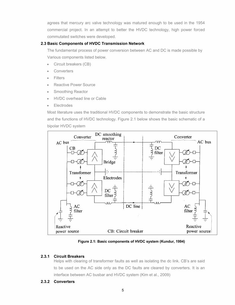
Most literature uses the traditional HVDC components to demonstrate the basic structure
and the functions of HVDC technology. Figure 2.1 below shows the basic schematic of a
bipolar HVDC system
Figure 2.1: Basic components of HVDC system (Kundur, 1994)
2.3.1 Circuit Breakers
Helps with clearing of transformer faults as well as isolating the dc link. CB’s are said
to be used on the AC side only as the DC faults are cleared by converters. It is an
interface between AC busbar and HVDC system (Kim et al., 2009)
2.3.2 Converters

6
It is said to be the most essential element for HVDC transmission (Kim et al.,
2009).The function of a converter is to convert electrical energy from AC to DC and
DC to AC (Sood, 2006).according to Siemens brochure dated march 2011, The
HVDC converters are mostly built as 12-pulse circuits made up of two 6-pulse
converter bridges connected in series. Figure 2.2 below shows such a setup.
According to V.K, Sood converters are basically configured in two types, namely
current source converters and voltage source converters. The latter will be discussed
in chapter 3
Figure 2.2: 12-pulse bridge (Siemens, 2011)
2.3.3 Filters As a result of power conversion process, harmonics are generated due to slicing of
voltages and currents, this then cause poor quality of supply (Sood, 2006).
Filters are there to mitigate harmonic voltages and currents generated by non-linear
converters. These harmonics have got the potential to cause overheating in
capacitors and generators. They also cause the interference with telecommunication
systems.
2.3.4 Reactive power Source These are usually in a form of capacitor banks or synchronous compensators .they
Compensates for the reactive power that the converter consumes during the
conversion process. I t has been noted that consumption of reactive power is much
higher under transient conditions. It’s very appropriate when connected to weak AC
networks.
2.3.5 Smoothing reactors The functions of smoothing reactors are nicely explained in (Arrillaga et al., 2007)
where it is stated that they decrease the harmonics in currents and voltages in the DC
line.by virtue of reducing the harmonic currents and voltages, the commutation
failures are reduced.

7
2.3.6 HVDC Overhead line or Cable The transmission of bulk energy takes place through cables and overhead lines (Kim
et al., 2009). More insight will be given to overhead lines due to the nature of this
thesis. Transmission lines are said to be mechanically designed for AC lines. The
main differences between AC and DC are insulation design, electric field
requirements and conductor configuration (Siemens broche, 2011).this implies that
the basic principle in determining overhead lines and towers are the same (Arrillaga
et al., 2007).
2.3.7 Electrodes Electrodes are electrical conductors that provide a reference potential point for the
HVDC system. These electrodes are said to be designed for normal operation as well
as fault conditions in HVDC systems (Arrillaga et al., 2007).
2.4 HVDC system configurations
HVDC system can be configured according to available flexible technology that fits
operational requirements and cost (Arrillaga et al., 2007). There are five basic
configurations illustrated in schematic diagrams and briefly discussed below.
2.4.1 Back-to-Back link This type of link is mainly used for power control, for instance when transmitting
power from one region to another under contractual basis.it is also the preferred one
when planning the transmission between asynchronous systems (Arrillaga et al.,
2007).converters are situated on the same site, this makes it to be more economical
as there are no transmission line or cable required. They are usually designed for
voltages between 50 and 150kV.
Figure 2.3: Back-to-Back link (Arrillaga et al., 2007)
2.4.2 Monopolar link The monopolar link has single conductor of negative polarity connecting converters at
each end. (Sood, 2006) explains the use of negative polarity as opposed to positive
polarity.in this configuration earth or sea is used as return path for current. According
to Arrillaga the ground return is rarely permitted in this set up due to corrosion and
magnetic interference problems. For this reason, metallic return is used.

8
Figure 2.4: Monopolar link (Arrillaga et al., 2007)
2.4.3 Bipolar Link The bipolar link has two conductors one is negative and the other one is positive.it
consists of two converters of equal ratings at each end. The earth electrodes are
connected right in the middle of converter stations. This is the most commonly used
configuration due to its capacity to be operated as monopolar link when one of its
links is faulty (Sood, 2006)
Figure 2.5: Bipolar link (Arrillaga et al., 2007)
2.4.4 Multiterminal links-parallel configuration
The multiterminal link has more than two sets of converter stations. The converter
function is apportioned as per network requirements where some will work as
rectifiers and some as inverters. Figure 2.6(a) and 2.6(b) shows the parallel and
series configurations respectively.

9
Figure 2.6(a): Multiterminal parallel connection (Arrillaga et al., 2007)
Figure 2.6(b): Multiterminal series connection (Arrillaga et al., 2007)
2.5 Applications of HVDC Systems.
The Traditional benefit of HVDC system is said to be bulk power transmission over long
distances however with the advances in power electronics, HVDC system is used in
various applications in the diverse energy industry. These benefits have been evaluated,
applied and endorsed according to technical and economic considerations in the
literature and electricity industry at large.

10
Figure 2.7: Different applications of HVDC systems (Kim et al., 2009)
2.5.1 Long Distance Bulk Power Transmission
HVDC has been found to be the cheaper option when transmitting large amount of
energy over long distances due to lower losses and cost than that of equivalent AC
line (Arrillaga et al., 2007).Encompassed on this benefit, the link is usually intended to
deliver from remote source to loading centre. The example of such link is Cahora
bassa (Mozambique) and Apollo here in South Africa.in this case the evaluation was
mainly concerned with cost of transmission. Figure 2.8 shows the variation of
transmission cost with distance of AC and DC lines. It has been noted that the
breakeven distance can vary depending on the per unit line cost. On overhead lines it
varies between 400 to 700 kilometres and between 25 to 50 kilometres with cables
(Sood, 2006). However we can see that beyond the breakeven distance, HVDC
shows the ability to transmit large amount of power with less capital cost and lower
losses than corresponding AC.

11
Figure 2.8: Cost comparison of AC/DC lines (Kim et al., 2009)
2.5.2 Possible Asynchronous Interconnections
With HVDC systems, the asynchronous operation is said to be possible between
regions having different electrical parameters (Frequency, Voltage, power etc.).
Figure 2.7 labelling number 4 demonstrates the HVDC’s ability to interconnect two
independent systems of different frequencies (50Hz system being connected to 60Hz
System).With AC links the Interconnections between power systems must be
synchronous. Thus different frequency systems cannot be linked. Security, reliability,
voltage and frequency control would be threatened by such operation if it were to be
applied on AC systems hence the HVDC system is the preferred option. Back-to back
links are frequently used for interconnection purpose.
2.5.3 HVDC Multiterminal systems
HVDC systems help with the transmission of power from remote generation areas
across various regions of the same country or different countries (Kim et al.,
2009).Some energy sources are often located far from the load centres e.g. Kaxu
solar plant in Northern Cape region of South Africa. If the intended use of power
generated by Kaxu Solar plant included Cape Town as well, HVDC would reliably
deliver electricity with low losses. It is further mentioned again that the interconnection

12
of two or more power systems can be exploited without adhering to AC common
rules.
2.5.4 Stabilization of Power Flow (Sood, 2006) indicates that the power flow can be uncontrollable in AC ties
particularly under disturbance conditions; this then leads to overloads and stability
problems. According to Arrillaga the DC link can be operated to improve the stability
of AC systems thereby modulating the power in response to the power swing. The
reversal of power flow is also achieved
2.6 Advantages of HVDC Systems
Each HVDC transmission link has its own requirements leading to it being the
technology of choice over AC system (Arrillaga et al., 2007). Some of the most
common benefits are listed below
Carries more power per conductor as compared to corresponding AC
No line length restrictions as there is no reactance in DC lines
Limit short circuit currents
Environmentally friendly as compare to AC
Ability to connect independent power systems
2.7 Classifications of HVDC technologies
According to ABB brochure dated August 2017, there are two types of HVDC namely the
traditional or classic technology that uses thyristors for conversion process and the voltage
source converter (VSC) technology that uses integrated gate bipolar transistors. The first
commissioned HVDC link was using line commutated current source converters (LCC). (K
Sood, 2006) mentions that it is possible to use line commutation (LC) or circuit commutation
(CC) techniques for the conventional thyristors. However due to direct dependence of the
firing angle alpha to the AC voltage, line commutation has been identified to absorb reactive
power from the AC system and therefore poses limitations to this technology.it is further
elaborated that power systems are subject to disturbances which lead to commutation
problems for the thyristor-based converters. Another limitation is the inability to control
reactive power (Sood, 2006).in search to overcome the line commutation limitations, forced
commutation or self-commutation were introduced. The circuit commutation artificially
generates voltage needed to achieve commutation. This thesis will make us of the voltage
source converter theory and it will be discussed in the next chapter.

13
CHAPTER THREE: VSC-HVDC TECHNOLOGY 3 3.1 VSC IGBT based Transmission
The fundamental current conversion process from AC to DC is achieved by means of
rectifiers and inverters. The conversion can be achieved by using natural commutated, circuit
commutated or self-commutated converters. According to (Sood, 2006), conventional
thyristors are called circuit-commutated devices and GTOs (Gate Turn-Off Thyristors), IGBTs
(Insulated Gate bipolar Transistors) and other such devices are called self-commutated
devices. The VSC-based power conversion provided a great flexibility in HVDC systems due
to its ability to provide reactive power in either direction at each end of the HVDC link
(Arrillaga et al., 2007). The first commercial VSC HVDC system was launched by ABB in
island of Gotland. ABB named this technology as HVDC light. The market is expanding as a
result Siemens and AREVA are the competitors offering similar technology named HVDC
plus and HVDC Extra respectively (Kim et al., 2009).The VSC IGBT based technology,
valves are built by IGBT and the pulse width modulation PWM) is used to create the desired
voltage waveform. A typical basic VSC interconnection is shown in figure 3.1 below followed
by component discussion.
Figure 3.1: VSC interconnection (Du; 2007);
3.1.1 Transformer Interface between AC system and converter thereby keeping secondary voltage level as
required by the converter. By adapting the converter voltage and providing the reactance
between AC system and converter unit, it is said that this operation controls the AC output
current. Spurred
3.1.2 AC filters The switching of IGBTs Inherently produces AC voltage output which contains harmonics.
Filters are necessary to eliminate the undesirable harmonics. Because the PWM technique
used in VSC eliminates low order harmonics, high pass filters are installed between the
transformer and the converter to mitigate high order harmonic content. Unfiltered harmonics

14
result in the malfunction of AC equipment, losses, Radio frequencies and telecommunication
(Du, 2007). The amount of filters installed in VSC is reduced as compared to LCC HVDC and
therefore cheaper.
3.1.3 Phase reactors Reactors also play a role in mitigating of high frequency harmonic content of the AC current.
They provide the control of real and reactive power flow thereby controlling the current
through it.
3.1.4 Converter configuration Converters are regarded as the main component of HVDC transmission as their primary
function is to convert electrical energy from AC-DC and vice versa. The basic configuration of
VSC is a two-level converter (figure 3.2(a)) which can be used in the building up of a three-
level VSC bridge (figure 3.2(b)) and subsequently multi-level converters (MMC).The
operation of the circuit requires the DC voltage to be maintained constant. This function is
achieved by installing DC capacitors and the switching is performed through IGBTs. The
free-wheeling diodes installed across each valve helps with the current diversion during
commutation if the main valves (Sood, 2006).series connection
Figure 3.2: VSC Configuration (Du; 2007)
3.1.5 DC link Capacitors DC storage shunt connected capacitor for the purpose of Keeping DC voltage within limits
and controls DC voltage ripple. The DC capacitor size is characterized as time constant:
τ (3.1)
It is defined as the ratio between the stored energy at the rated DC voltage and the nominal
apparent power (Du, 2007); where

15
C= Capacitor
=rated Dc voltage
S = nominal apparent power of the converter
3.1.6 DC cables / Overhead transmission line Transmitting medium from one point to other .The developments in XLPE cables made VSC
HVDC transmission even easier. The previous technology that suffered from moisture or
water ingress is now replaced by DC cables with insulation of extruded polymer. There are
no length limitations as compared to the corresponding AC cables. Cables are more
preferred than overhead lines due to effects imposed by overhead line on the environment.
3.2 Advantages of VSC Based Transmission
The self-commutated VSC based transmission has several advantages which lead to it being
the most competitive at transmission distances of over 100km and power levels between 200
and 900 MW.
It has the ability to generate and absorb reactive power independently from Active
power flow.
It significantly reduces the generation of harmonics.
No AC system voltage source needed for commutation
It eliminates problems of over-voltages
3.3 Applications
The advantages mentioned in 3.2 made the following application possible with regards to
VSC HVDC (Kim et al., 2009).VSC HVDC is the preferred system for use in various
transmission applications, using overhead lines, land and sub-marine cables or back-to-back
connection (ABB Brochure, August 2017)
3.3.1 Power provision over long distances through transmission lines Electricity generating sites are often situated far from consumers; electricity must cross long
distances to get where it is needed. According to literature and ABB HVDC is the most
reliable and efficient way of getting it there. Caprivi link connecting Zambezi and Namibia is a
reference project where 350km long overheard line of about 350kV DC was built
3.3.2 Energy provision in urban areas experiencing rapid load growth Urban loads are increasing and businesses are continuously increasing their power loads in
order to meet the demand. This in turn is overloading the existing AC network. Acquiring the
land for new electricity infrastructure has become a challenge. Also the environmental effect
posed by transmission lines is another hick-up. It has been noted that urban electrical system
require easy solutions that can be attained within urban boundaries and shot lead times.
Replacement of existing AC overhead lines with DC cables is said to be an opportunity to
use same ROW and get 2-3 time more power than comparable AC system (ABB Brochure,

16
August 2017).another reference project is a link connecting Long Island and Connecticut in
new York
3.3.3 Delivering energy to independent systems ABB further educates us on the coupling of previously separated electricity markets and ever
increasing commercial interconnections especially with the integration of renewable energy.it
is precisely stated that in order to operate effectively, these interconnections will require
controllable power flows. Having different characteristics between renewable energy and
traditional energy mix, controllability and flexibility of power flow is a requirement. VSC HVDC
offers the frequency and voltage regulation, emergency power support, stability
enhancement, power flow control. These are all features needed for integration between
these two systems.
3.3.4 Interconnections Liberation of energy markets resulted in dozens of electrical interconnections across the
continents in the world. These are helping to create secure and sustainable supply of
electricity. VSC HDVC is said to be the possible technical solution especially when
interconnecting countries of different frequencies.
3.4 Comparison of VSC HVDC and LCC
The VSC was initially used in low voltages by industries for motor drives providing fast
desirable continuous control of frequency and voltage magnitude. Due to this perception and
other advantages presented by LCC, Most of present HVDC transmission networks use LCC
technology. The first commercial HVDC link mentioned in 2.2 uses the LCC technology. The
LCC HVDC uses thyristors in a current source converter (CSC) topology. With the advent of
solid-state electronics and the silicon-controlled rectifier, the development of thyristor valve
converter began to replace mercury arc-valve converters. Thyristor valves completely
replaced mercury-arc valves due to their strong features, reliability, low maintenance, and
cost and gave real momentum to HVDC.The use of Thyristor based switches provided HVDC
flexibility however it is said to be restricted by switching characteristics of silicon controlled
rectifier. Thyristors can only switch off when the current through them becomes zero and its
commutation process depends on the normal operation of AC grid. Another restriction is the
delayed firing of thyristors that result in the current lagging the voltage and thereby reactive
power abortion by the HVDC link. It is said that the power direction can be changed if DC
voltage is reversed which turns to be a time consuming operation.
For these inherent limitations LCC HVDC is feasible for long distance transmission at extra
high voltages. This further necessitated more research as Dr Hans-joachim Knaak from
Siemens mentions the HVDC/FACTS challenges ahead. he articulates that HVDC will move
from being an isolated point-to- point connection to being an integrative part of the grid where
there will be a need to overcome the above mentioned Inherent LCC HVDC limitations.

17
The VSC IGBT-based Transmission technology presented more advantages than LCC
HVDC technology. The IGBTs used in VSC scheme can be switched on and off so many
times per cycle. Their operation is not limited by zero crossing current and the operation of
the surrounding AC grid. According to (Arrillaga et al., 2007), VSC does not suffer from
commutation failures. There is no reactive compensation required as the VSC can control the
feeding and absorption of power in to the system. Other added advantages are the
bidirectional power transfer without polarity reversal, compact design, black start capabilities
and less filters. VSC technology can be connected to the network in many different ways
depending on the particular application. It is not only limited on long distance transmission. It
fulfils a situation where HVDC systems can be applied and expanded in a manner similar to
AC substations ( Andersen , 2013:4)
3.5 Operating principle of VSC
Two-level single phase VSC in figure 3.3 below is used to demonstrate the operating
principle of VSC. The two-level was chosen due to proven technology, simplicity and the fact
that it allows the IGBTs to be connected in series depending on the required supply voltage.
The converter valves and transformers are assumed to be lossless with negligible ripple on
DC capacitors. Since the inherent conduction in solid-state switches is unidirectional,
freewheel diodes are connected in parallel to eliminate negative voltage across the load,
while current flow in both directions. The basic principle of single phase two-level VSC where
switching circuit and corresponding voltage wave form are shown in figure 3.3.It can be
noted that the AC terminals are switched in a bipolar manner between voltage levels of +Vd
and-Vd
Figure 3.3: Basic Operation of two-level VSC (Arrillaga et al., 2007)
The four possible current paths are shown in figure 3.4

18
Figure 3.4: Current Path in a two-level VSC (Arrillaga et al., 2007)
When the upper switch is closed the output voltage is +Vd/2 and the flow of current is
demonstrated on figure 3.4(a) and 3.4(b).when the lower switch is on the output voltage is -
Vd/2 and the flow of current is shown on figure 3.4(c) and 3.4(d).uncontrolled rectifier is
formed when both switches are blocked, in this state the external AC voltage charges the DC
capacitors to the peak value.it has been noted that a fully charged DC capacitor together with
connection of external sources can kick start the operation of VSC.
3.6 Power Transfer in VSC
VSC was initially built for transmission and sub-transmission power transfer of between 5 to
150MW however due to availability and increasing power ratings of IGBT, the VSC power
capabilities are in hundreds of megawatts. VSC-based HVDC has the ability to control power
in the system. The operation of the switches ought to block a unidirectional voltage yet be
able to conduct current in either direction when bidirectional power flow is required. The
Active and reactive power components are expressed as:
(3.2)
(3.3)
Where:
V1= is the system AC Voltage,
V2is the VSC output voltage,
δ the phase angle
X reactance between V1 and V2
According to arrillaga, if the converter is connected to an active DC network, a four quadrant
operation can be achieved as shown on figure 3.5 below. In this operation the converter can
act as a rectifier or inverter with leading or lagging reactive power. The flexibility offered by
VSC allows the operation at any point within the circle.

19
Figure 3.5: VSC Four-quadrant operation (Arrillaga et al., 2007)
It has been confirmed that when changing the amplitude between the converter bus voltage
and the valve bus voltage control the reactive power flow between the valve and transformer
bus and consequently between the converter and the AC network (ABB brochure, 2017).The
phasor diagram in figure 15 illustrates the operating mode of VSC as a reactive power
controller Where :
V2 = V1; I=0
V2 > V1; I leads V by 90
V2 < V1; I lags V by 90
When V1 is equal to V2 in the converter voltage V2 and AC system voltage V1 are in phase,
the VSC operates as reactive power compensator. There is no exchange of reactive power
between converter and the system.in this mode, the current is said to be zero (I=0).When V2
is greater than V1 the current leads voltage by 90 , here the converter generates and supply
reactive power into the system. When V2 is less than V1 the current lags the voltage by 90 ,
here the converter absorbs the reactive power from the system. Thus the VSC scheme can
operate as power transmission system or two independent STATCOMS if there is no power
available of required.

20
Figure 3.6: VSC Phasor diagram for reactive Power Control (Arrillaga et al., 2007)
3.7 VSC PWM Methods
Pulse width modulation is characterized by high-frequency switching of the fixed DC voltage
where output waveform is filtered to produce specified fundamental component of
controllable magnitude.in this process the lower order harmonics are eliminated by
modulating the width of voltage pulses (Arrillaga et al., 2007).
The PWM method used in the operation of VSC is said to have an advantage of
instantaneously controlling the voltage magnitude and phase. Furthermore it provides
different types of schemes to generate PWM patterns amongst them are Space vector,
triangular-wave and trapezoidal modulation. It should be noted that the most accurate
scheme of the PWM pattern may not necessarily be the optimal choice.one should always
evaluate the economic, harmonic and switching losses aspects when choosing the scheme.
Tabulated below is the comparison on the PWM schemes. When applying a VSC
technology, the objective is coupled with minimising harmonics as much as possible,
reduction of losses and low cost.
Table 3.1: Evaluation of PWM schemes (Kim et al., 2009)
Aspect Space-vector Triangular-wave Trapezoidal
Harmonics Small Medium Large
accuracy Large Medium Small
economics Large Medium Small

21
According to (Arrillaga et al., 2007) the use of VSC pulse width modulation in power
transmission is practical if the Three phase system is symmetrical and the output waveform
should contain only odd harmonic orders. The choice of modulation principle is governed by
three ratios namely frequency, control and utilisation ratios. These ratios are mathematically
expressed as
(3.4)
Ѵ
Ѵ (3.5)
Ѵ
Ѵ(3.6)
Where: p is the frequency ratio
fpis the modulation frequency
fis the output frequency
is the control ratio
Ѵ is modulated waveform
Ѵ is the unmodulated waveforms
is the utilisation ratio
Ѵ is the maximum available voltage
Frequency ratio is defined as the ratio of modulation frequency to the output frequency.
Control ratios are the ratio of the fundamental components of modulated to unmodulated
waveforms and lastly the utilisation ratio is a measure of how well the modulation principle
uses the maximum available voltage. The quality of supply offered by transmission and
distribution networks ought to be free from harmonics. The waveforms needs to be further
improved by means of AC filters and series reactors. From the various PWM schemes
mentioned above, the incorporation of optimal pulse width modulation (OPWM) technique
would be beneficial to reduce converter losses and elimination of harmonics. The effects of
OPWM are illustrated in the figure below where fundamental component is shown as the
dotted line and the phase to ground converter terminal voltage.

22
Figure 3.7: Harmonic cancellation through VSC-PWM (Arrillaga et al., 2007)
When the VSC using PWM is designed for optimal cancellation of harmonics, the individual
harmonics are said to be reduced to 1 percent and the total harmonic distortion (THD) is
reduced to 2.5 percent. The harmonics are concentrated in a narrow bandwidth. PWM –VSC
technology provides :
Frequency control: by regulating power delivered to or taken from the AC system.
AC voltage control: by regulating the magnitude of the fundamental frequency component
of the VSC output AC voltage on the converter side of the transformer.
Active power control: by regulating phase angle of the fundamental frequency component
of the converter –generated AC voltage.
Reactive power control: by regulating magnitude of the converter AC voltage source.
DC voltage control: by regulating power required to charge or discharge the capacitor to
maintain specified DC voltage level.

23
3.8 VSC HVDC System Control
The intended purpose of VSC with regards to this thesis is to control active and reactive
power while keeping a constant voltage at the DC terminals. VSC can be controlled in four
controlled modes depending on the desired outcome. Below are the control modes:
Active power control mode
Reactive power control mode
AC voltage control mode
Constant DC voltage control mode
These control modes are taking place in VSC internal structure shown in figure 3.8 below.
Figure 3.8: VSC internal control structure (Ruihua et al., 2005)
The VSC control structure consists of outer control loop and inner control loop. The outer
loop controllers are project specific. The Voltage at AC terminals, reactive power and active
power at rectifier side are all controlled by outer loop. The controller can alternate between
controlling the reactive power and AC bus terminal voltage as shown in figure 3.9 below. This
is achieved by employment of PI controllers within the outer and inner loop controllers,
Where a proportional gain and an integral gain controls the desired value to a given
reference value in this form
(3.7)
Where is the proportional gain and is the integral gain.

24
Figure 3.9: Reactive power and AC voltage controller (Imhof, 2015)
According to (Imhof, 2015) the inner control loop controls the currents to the reference values
received from outer loop. Today’s VSC-HVDC schemes are designed to keep DC voltage
fixed and the control of AC voltage output is varied by means of a modulation index signal
(λ).direct control and vector control are the two possible approaches to implement
modulation index. In figure 3.10, it can be observed that the modulation index or phase angle
is adjusted directly from the parameters being controlled, while in figure 3.11 the currents
components are first transformed to d-q axes, which are then synchronized with AC system
Voltage through phase-locked loop (PLL).this current loop is said to be slowing down the
desired response speed as the d-q voltages generated by vector control are transformed in
to three-phase quantities and converted into line voltages by VSC. However it protects the
valves from overloading (Arrillaga et al., 2007).
Figure 3.10: Direct Control of Modulation Index (Arrillaga et al., 2007)

25
Figure 3.11: Vector control via d-q axis (Arrillaga et al., 2007)
The conversion of three-phase sinusoidal system is achieved by applying Park’s
transformation matrix. Within the Park’s transformation matrix there is an intermediate α-β-0
transformation and the phase rotation matrix transformation which then result in d-q-0 frame
control. This is represented in 3.8 below.
(3.8)
Where is the parks transformation matrix aiding the reproduction of d-q-0 terms .The
whole transformation is done to prohibit the three-phase sinusoidal system from being time
variant. This means they are transformed into DC terms. At the end of the transformation
process, it ought to be noticed that in a VSC, through d-q-0 change, the amounts are
changed over to DC constants.
3.9 Conclusion
The VSC HVDC technical aspects were discussed where it became clear from the
advantages and applications that VSC HVDC has interesting qualities. The basic and
different methods of operation were highlighted, the incredible progress in fast switching
devices like IGBTs has encouraged the interest in the study of shunt and series filters. As a
result of PWM inverter technology together with “d-q theory” power filters can now be used in
industrial field. The stand-alone feature of the ability to control the transfer of reactive power
as well as terminal voltage has made VSC IGBT-based technology an attractive option for
HVDC transmission.

26
CHAPTER FOUR: AC to DC CONVERSION
4 4.1 Changing the Power Pool Requirements
South Africa’s main source of electrical energy is generated from Fossil Fuels. However the
development of existing and future generation power pools to meet the Countries energy
demand by 2030 was analysed taking into account three potential main generation pools
namely, underground coal gasification, nuclear power stations, and gas supplemented by
renewables. The generation power pool triggered the strategic analysis of the requirements
of the future power corridors to meet the expected load growth and integrate the potential
future generation scenarios. The approach was to design the different power corridors to be
as independent of other power corridors and generation scenarios as possible. The major
advantage of this approach was the flexibility to respond to different generation scenarios
that may eventually manifest.
Economic and technical evaluation was done where HVAC and HVDC transmission lines
were proposed at different voltage levels to achieve the desired power corridor. However due
to current generation surplus, country’s financial status ,political influence and other factors,
The anticipated generation power pool differed from original plan. This had an impact on
proposed power corridors in such a way that some of the sub-transmission projects were put
on hold. It must be noted that the load continues to grow and the present HVAC sub-
transmission network cannot handle the load demand. Certain areas cannot add new
customers to the grid due to network that already suffers from low voltages, thermal loading
and instability. Certain existing transmission lines should be considered for recycling from a
single circuit to a double circuit structure, larger conductor bundles or higher voltages. The
enhancement of existing power transmission capacity of the lines through DC will be studied
in this chapter.
4.2 Converting AC lines into DC
As part of the capacity enhancement in the existing transmission networks, it makes more
sense to utilise the existing transmission infrastructure as opposed to building new
transmission network that will take time to be developed. Converting HVAC overhead lines
into HVDC might provide a significant increase in transfer capacity for a relatively little cost
less time and little environmental impact. It has to be noted that before the conversion of AC
into DC line, certain conversion criteria has to be met. This includes the thorough analysis of
existing AC line where most critical electrical parameters, structures, protection and
environmental aspects are evaluated for the alignment with HVDC. Different conversion
topologies and criteria will be discussed as follows.

27
4.2.1 Single Circuits AC lines According to (Larruskain et al., 2014) article, Single circuits AC lines can be adapted to
bipolar, tripolar and modulated bipolar DC lines. The article puts more focus on single circuits
as it stipulates that they are the more complex ones when it comes to conversion due to its
odd number of conductors. When the single circuit AC line is converted to bipolar DC line,
the HVDC line will have three circuits with one conductor per pole. However it must be noted
that the proposed VSC technology has two poles with opposite polarities as seen in chapter
3 figure 3.3, as a consequence a conductor per pole is used leaving one spare conductor
which can be used as return conductor in emergency situations. Figure 4.1 below shows the
VSC based HVDC configuration.
Figure 4.1: VSC based HVDC Line (Larruskain et al., 2014)
Looking at the capacity enhancement, the power transmitted by the adapted DC line is
2 (4.1)
Where:
= is the power transmitted by converted DC bipolar line
is the pole-to-ground voltage
is the rated current of both poles
Another method of single AC line conversion is the modulated bipolar DC line, in this
configuration there is a positive pole, negative pole and the third pole changes polarity
between negative and positive as required by the system. All three conductors are in use
with one conductor per pole as shown in figure 4.2 below. It can be seen that the positive
and negative poles are the outermost conductors and the polarity of the middle conductor is
commutated with IGBTs.

28
Figure 4.2: VSC based Modulated Bipolar DC line (Larruskain et al., 2014)
According to (Arrillaga et al., 2007) the modulated DC transmission was introduced as an
effective way of achieving the maximum power carrying capacity by making use of third
conductor in bipolar configuration. The modulated bipolar system can be configured in such a
manner that one conductor is sending and the other two are return conductors and vice
versa. (Larruskain et al., 2014) states that if the bipolar configuration has one sending
conductor, it is overheated due to the fact that it withstands a higher current that it’s rated
value. While the two return conductors share the current and consequently operate lower
than rated current. This operation is shown in figure 4.3 where sequential alternate between
High current state and low current state is demonstrated.
Figure 4.3: Operation of Modulated Bipolar DC Line (Larruskain et al., 2014)
This configuration is capable of transmitting 1.26 times higher power than bipolar
configuration. The power transmitted is defined by:
1.26 0.63 0.63 (4.2)
2.53

29
1.26
Where 1.26 is the high current state at pole 1 and 0.63 is the low current state at pole 2
and 3.
The third method is the adaptation of single AC line into tripole DC line. This configuration
also makes use of all three conductors. There is positive pole, negative pole and the third
pole which changes polarity.it is said that this system was originally implemented with LCC
converters as a result the third pole is connected to thyristor based system as shown figure
4.4
Figure 4.4: VSC based Tripolar DC line (Larruskain et al., 2014)
The distinct characteristic of this configuration is that all conductors use their full thermal
capacity unlike on modulated bipolar where only one conductor would experience
overheating due to exceeding rated current. Positive and negative pole alternate between
high current state and low current state while pole 3 is said to be reversing its polarity
periodically, sharing positive and negative current with poles 1 and 2.the operation is shown
in figure 4.5 below. This configuration is capable of transmitting 1.37 times higher power than
bipolar configuration. The power transmitted is defined by:
1.37 0.37 (4.3)
=2.74
= 1.37
Where 1.37 is the high current state at pole 1 and 0.37 is the low current state at pole 2
and is the rated current of pole 3.

30
Figure 4.5: Operation of Tripolar DC Line (Larruskain et al., 2014)
From the three different adaptation methods discussed above, Bipolar system is seen as the
most simple and economical configuration. However from the Power formula in (4.1) it can
be seen that it transmits less power than Modulated bipolar and tripolar systems. The bipolar
configuration operates similarly to the tripolar configuration but one needs to take note of the
third pole that that uses thyristor based system on the latter.
4.2.2 Double Circuits AC lines Double circuits AC lines consist of six conductors. This type of configuration can be adapted
to three bipolar DC circuits. This is said to be the most productive method of conversion.
Each circuit will consist of conductors (Arrillaga et al., 2007).The power that can be
transmitted by AC line is defined by
(4.4)
The corresponding DC line can transmit:
(4.5)
Adapted Double circuits DC line can transmit up to three times the power transmitted by
bipolar system.
4.2.3 Insulation Insulation is considered as one of the most important aspects when converting an AC line to
DC line. According to Kim et al., 2009 Insulation ascertains the number of flashovers to be
expected on a statistical basis thereby ensuring the reliability of the DC line. Insulation must
be properly selected such that it withstands overvoltage’s that resembles switching surges,
flashovers due to contamination, lighting overvoltage and adverse environmental conditions.

31
Selection and sizing of line insulation is governed by the ratio between the continuous
working withstand voltage between AC and DC systems. For a given insulation length, the
ratio of continuous working withstand voltage is
(4.6)
Kim et al., 2009 states that the environmental conditions of the route of the line have a
conclusive influence on its reliability. Insulation contamination can be caused by the
presence of polluted air, dew, fog etc. all these have major influence on the occurrence of
flashovers. Arrillaga 2007 additionally notes that if a line is passing through a reasonably
clean area kmay be as high as √ , corresponding to the peak value of rms alternating
voltage. However (Larruskain et al., 2014) confirms that from the past experiments, a ratio of
should be considered on overhead lines due to unfavourable effects of pollution on
insulators. For cables is at least 2.
Switching surges occur in a bipolar HVDC overhead line due to one pole experiencing a
conductor-to-pole flashover (Kim et al., 2009). The potential of the other pole is said to be
elevated. This in turn causes over voltages. With that being noted, (Arrillaga et al., 2007)
suggested that a transmission line has to be insulated for over voltages during faults and
switching operations. To properly select and size the insulation, the AC lines need levels of
insulation corresponding to an AC voltage of 2.5 to 3 times the normal rated voltage as
shown in equation below.
. (4.7)
In contrast with suitable converter control, the corresponding DC insulation ratio is
.
(4.8)
It can be seen that the relationship between DC pole-to-ground voltage ( ) and the AC
phase-to-ground voltage ( ) exist.
(4.9)
∗ (4.10)

32
Apart from ensuring the reliability of the DC line, Outdoor insulators are known for isolation of
conductors from towers. Three types of insulators are classified into porcelain, glass and
composite. Figures 4.6-4.8 show the kinds of outdoor insulators.
Figure 4.6: porcelain insulator (He , 2013)
Figure 4.7: Glass Insulator (He , 2013)
Kim et al., 2009 states that there has been a debate in the in the industry with regards to
relative merits of glass and porcelain caps. There were claims that when the porcelain
insulator surfaces are wet, water tends to form a continuous film which could lead to
significant decrease in surface resistivity. Glass insulators were identified as prone to fracture
under stress. With improved design the glass insulators were seen as stronger that porcelain
insulators due to their immunity to erosion. Additionally it is believed that it is easy to notice
defects in glass insulators while they remain invisible in porcelain cap and pin. Nevertheless
these two are said to be equivalent.

33
With the advancement in technology, Composite insulators were introduced to eliminate the
effects of pollution thereby preventing line flash-overs. They have shown excellent behaviour
in polluted areas. They came in reduced weight and high creepage on short length when
compared to porcelain and glass. The distinct characteristic of composite insulators is the
hydrophobia of the surface. No water film is formed on its surface .this type of insulator has
been used in HVDC for more than a decade and it is supposedly the future insulator.
Figure 4.8: Composite insulator (He , 2013)
4.2.4 Conductors In most adaptations of AC lines to DC lines, same conductor is used.it should be noted that
the choice of the conductor depends largely on corona and field effect considerations. It has
been reported that corona and field effects do not institute an exceptional problem for DC
voltages up to 1200kV.
4.2.5 Right of Way The process of acquiring land for the new transmission corridors can be expensive and
lengthy. On each project it is advisable to consider alternatives of more favourable routes
from the point of view of wayleaves and any other limiting factors in the occurrence of faults.
For a given transmission capacity of 10 Gigawatts (GW) The space requirement of HVAC
overhead lines can be four times higher than that of corresponding HVDC lines. If we take a
look at figure 4.9 below, the 800 kV HVAC line would require a width of 425 meters when
transmitting power via a link of 10 GW. While the HVDC line of the same capacity would only
require a width of 100 meters (Teske et al., 2015).With HVDC overhead lines, only two
towers and less number of conductors compared to corresponding HVAC which uses five

34
towers with significant more conductors. A cost saving in material is also achievable with
HVDC technology.
Figure 4.9: ROW comparison (Teske et al., 2015)
4.2.6 Clearance Most of the existing HDVC lines are of bipolar configuration. The heads of the adapted
towers ought to keep the required minimum clearance. It should be noted that the minimum
clearance for conductor-to-ground must be adhered to as per national standards, not
forgetting the maximum conductor sag at the maximum continuous current. Overhead AC
system towers are over dimensioned; this makes the new DC voltage to comply with
regulatory requirements as it is commonly within required clearance limits. However if the
existing towers do not meet the minimum required clearances, a reconstruction may be done
in a form of changing cross arms (Larruskain et al., 2014).one must bear in mind that the
cost of reconstruction must always be less than the cost of erecting new towers. The figure
below shows minimum clearance in air as a function of overvoltage factor.
Figure 4.10: Minimum clearance in the event of flashover due to overvoltage (Kim et al., 2009)

35
4.2.7 Environmental Effects Utilities and engineering profession at large have an obligation to conserve and protect the
environment in their business undertaking. Environmental effects posed by overhead
transmission lines have been a concern lately. Electric field, Radio Interference, noise and
visual impact are the major points of concern.
4.2.7.1 Electric field
In overhead lines, electric field is caused by the potential difference between the conductor
and earth and the space-charge clouds produced by conductor corona (Arrillaga, 1998).In
conductor cables the effects of corona were found to occur at voltages as low as
approximately 15kV/cm (Kim et al., 2009).In case of overhead lines, the highest electric field
strength that occurs is approximately 21kV/m for a given 450kV power line in figure 4.11.The
electric field problem is less precautious in DC due to lack of steady-state displacement
current. The critical point where ionization can start to occur due to field strength has been
determined to be 29.8kV/cm.
Figure 4.11: Electric field for both monopolar and bipolar lines (Arrillaga, 1998)
4.2.7.2 Corona, Radio Interference and audible noise
Kim et al., 2009 defines corona as the electric discharge with luminous phenomena as a
result of the ionization of the air surrounding a conductor. This usually occurs in a non-
uniform electric field when the field strength exceeds a critical value. Radio interferences and
audible noise are primarily caused by corona discharge.

36
CHAPTER FIVE: VOLTAGE STABILITY 5 5.1 Stability concepts and definitions
Power system stability as defined by IEEE/CIGRE joint task force is the ability of an electric
power system, for a given initial operating condition, to regain a state of operating equilibrium
after being subjected to physical disturbance, with most system variables bounded so that
practically the entire system remains intact (Kundur et al., 2003).Power system instability has
traditionally been limited to synchronous machines to remain in synchronism. However the
instability issues are not limited to loss of synchronism only, voltage or load instability may
lead to power system instability problems. Voltage stability is defined as the ability of a power
system to maintain a steady acceptable voltages at all buses in the system under normal
operating conditions and after being subjected to a disturbance (Kundur, 1994).
The fast short circuit clearing and powerful excitation system has managed to overcome the
synchronization problem. Utilities, researchers and planning engineers are now concerned
with voltage stability being the leading factor to limit power transfers. Today’s power system
is being operated closer to stability limits due to economic and environmental constraints and
this poses a threat to power system security. Power system is said to have entered a state of
voltage instability when a disturbance, increase in load demand causes a progressive and
uncontrollable drop in voltage (Kothari & Nagrath, 2011), (Kundur, 1994).
The principle of voltage stability says that at a given operating condition for every bus in the
system, the bus voltage magnitude must increase with an increase in reactive power
injection at the same bus. The system is said to be unstable if for at least one bus in the
system, the bus voltage magnitude decreases as the reactive power injection at the same
bus increased (Kundur, 1994).Consequences of events accompanying voltage instability
may lead to voltage collapse, a process by which voltage instability leads to loss of voltage in
a significant part of the system.
According to book written by Prabha Kundur, Voltage instability may occur in several
different ways. a representation of simplified radial feeder or load area served by a large
system through transmission line is demonstrated through figure 5.1.The two terminal
network consisting of a constant voltage source (ES) feeding the load (ZLD) through series
impedance (ZLN) can explain a simple case of voltage stability (Kundur, 1994). The current
expression is given by
(5.1)
∠ ∠

37
The magnitude of the current is given by
This may be written as:
√ (5.2)
Where:
The magnitude of the receiving end voltage is given by
√ (5.3)
The power supplied to the load is given by
(5.4)
Figure 5.1: Voltage stability phenomenon (Kundur, 1994).
The picture of simplified voltage stability phenomenon in figure 5.2 is drawn by plotting
receiving end voltage( ), current ( ) and power ( )as a function of load demand .As
the load demand increases by reducing load impedance, the power supplied to load
increases rapidly in the beginning then slowly before reaching a maximum. The power plot in
green shows that there is a maximum value of active power that can be transferred through
impedance from a constant voltage source. The reduction in load power takes effect due to
load impedance being less than series impedance which then results in the receiving end
voltage.

38
When the maximum power reaches a critical value, a critical operating condition is
experienced. The correspondence between critical value and maximum power represents
the limit to sufficient operation. For hire load demand, reducing power by means of reducing
load impedance would result in unstable system as the load characteristics govern the
system stability. With respect to constant impedance static load characteristics, the system
stabilizes at power and voltage levels lower than desired values. While with constant power
load characteristics, the instability is caused by collapse of the load bus voltage.as it was
mentioned earlier that the driving force for voltage instability is usually the load
characteristics.it can be seen that most of the instability issues are due to load stability which
is sometimes called voltage stability. Though this phenomenon is not limited to load stability,
other characteristics are due to transmission line and transformer effects (Kundur, 1994).
Figure 5.2: Receiving end voltage, current and power (Eskom, 2013)
Conceptual analysis of voltage stability is also shown through traditional P-V curves in figure
5.3.The various values of power factor are plotted where higher voltage solution indicates
stable scenario while the lower voltage solutions indicates unstable operation. The locus of
critical point is observed and shown through dotted line. This is the point where the system
experiences the maximum power and critical voltage. All the points above critical points
represent the system’s satisfactory operating condition

39
Figure 5.3: P-V curve for the analysis of voltage stability (Kundur, 1994)
5.2 Classification of Voltage Stability
Voltage stability is classified into four categories namely: large disturbance voltage stability,
small disturbance voltage stability, Short term and long term voltage stabilities. The literature
defines voltage stability according to sizes of disturbances, system states and time frames. A
short outline of the groupings is shown in figure 5.4
Figure 5.4: Groupings of Voltage instability (Taylor, 1994)
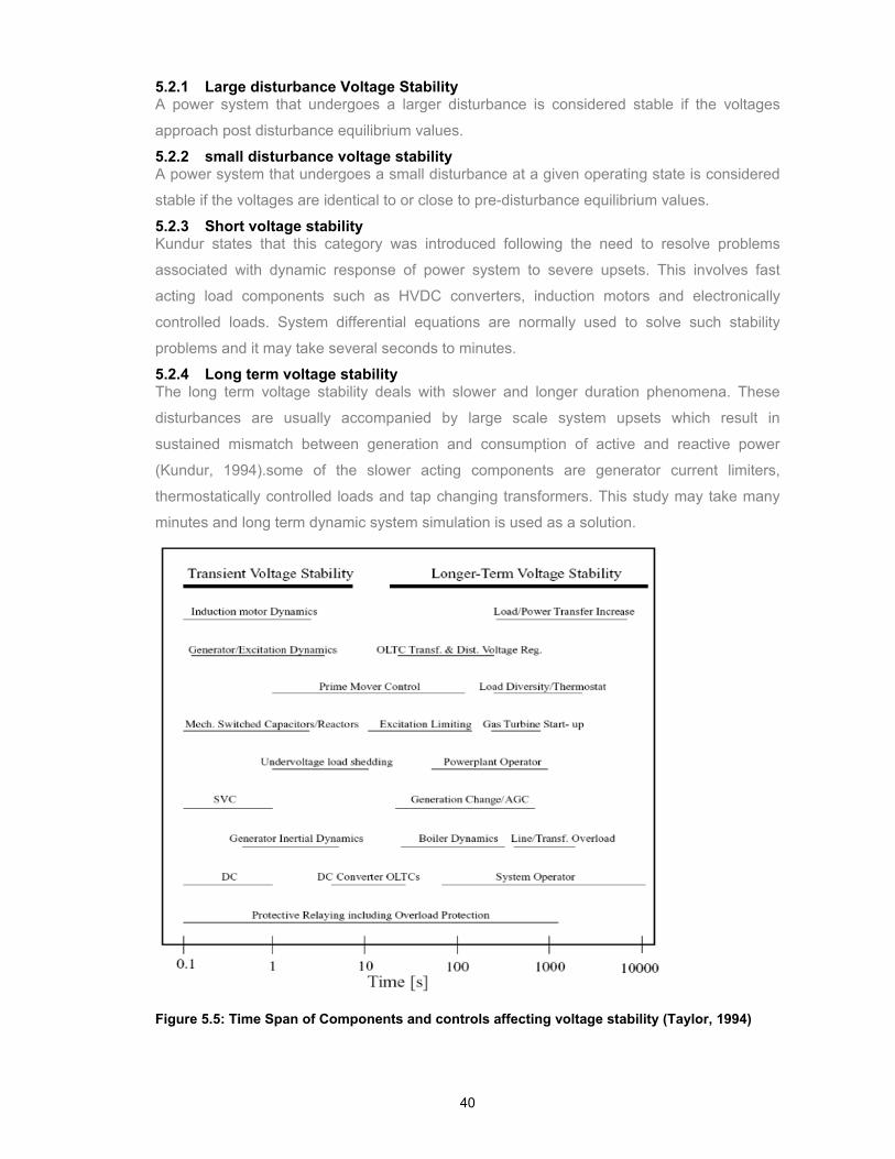
40
5.2.1 Large disturbance Voltage Stability A power system that undergoes a larger disturbance is considered stable if the voltages
approach post disturbance equilibrium values.
5.2.2 small disturbance voltage stability A power system that undergoes a small disturbance at a given operating state is considered
stable if the voltages are identical to or close to pre-disturbance equilibrium values.
5.2.3 Short voltage stability Kundur states that this category was introduced following the need to resolve problems
associated with dynamic response of power system to severe upsets. This involves fast
acting load components such as HVDC converters, induction motors and electronically
controlled loads. System differential equations are normally used to solve such stability
problems and it may take several seconds to minutes.
5.2.4 Long term voltage stability The long term voltage stability deals with slower and longer duration phenomena. These
disturbances are usually accompanied by large scale system upsets which result in
sustained mismatch between generation and consumption of active and reactive power
(Kundur, 1994).some of the slower acting components are generator current limiters,
thermostatically controlled loads and tap changing transformers. This study may take many
minutes and long term dynamic system simulation is used as a solution.
Figure 5.5: Time Span of Components and controls affecting voltage stability (Taylor, 1994)

41
5.3 Parameters affecting voltage stability
Voltage instability may emerge because of numerous reasons; some significant contributors
are listed below.
Increase in Load
Switching of heavy loads
Long transmission lines and line tripping
Action of tap changing transformers
Loss of synchronism (generator related parameters)
Changes in speed prime mover
5.4 Mitigations of voltage stability
According to (Kothari & Nagrath, 20011), Voltage stability can be enhanced by the
accompanying means.
Erecting an additional transmission line
Compensating the line length
Enhancing the reactive power support by installing SCV and C-banks
Enhancing excitation generators
Introduction of HVDC tie between regional grids
Last resort should be strategic load shedding
5.5 Stability concerns posed by DG in Distribution Network
Chapter five addresses system stability for Master sub-transmission network. Markus, 2015:
IV notes that the Europeans simulation studies have shown network stability improvements
when VSC HVDC link is incorporated into the sub-transmission network. He further says the
improvement is noticeable even with small transmission capacity networks. However South
Africa is the late adopter of the distributed generation and conversion of AC to DC lines and
therefore had some stability concerns with regards to application of HVDC systems on sub-
transmission and distribution networks.
The power system was designed through a top down approach with the synchronous
generators connected at the transmission network and operated to transport large amount of
active and reactive power from generation, through transmission, to the distribution network
and eventually the load. The control of voltage and frequency thus was done on the
transmission network by the system operator. Through the introduction of DG, the distribution
network will be having generators connected on the high voltage (HV), medium voltage (MV)
and low voltage (LV) system. This creates the previously passive network into an active
network, with bidirectional power flow.

42
5.5.1 Voltage Stability Concern Concerns were raised where voltage stability with embedded generation and sub
synchronous resonance with wind turbines on series compensated lines were the most
worrying aspects. The distribution network’s reactive power supplying elements are lines,
shunt capacitors, voltage regulators and On-load Tap Changers. Now with distributed
generators of varying generator technologies such as photovoltaic systems (PV), wind
turbines (WT), gas turbines, concentrated solar plants (CSP), and hydro power plants
integrating into the network, the implications of inefficient control will have an impact on
voltage regulation and losses. A typical distribution network with power flow of the feeder
using standard control of the on-line tap changers (OLTCs) and voltage regulators (VRs) is
shown if figure 5.6.
Figure 5.6: Distribution feeder with Voltage regulator (Eskom, 2013)
Figure 5.7. below shows the power flow for a feeder with varying size DG. The reverse power
flow will impact the network and the control of the combination of the existing equipment and
the newly connected DG brings uncertainties.
Figure 5.7: Distribution feeder with Power flow for varying levels of DG penetration (Eskom, 2013)
A number of factors to be considered when integrating DG were brought forward namely: current carrying capacity of the line at given temperature ∆ change in voltage caused by DG integration Rapid voltage change(RVC) limits as specified on South African Grid Code (SAGC) ( ) Maximum and minimum operational voltages.

43
Theoretical values were used to roughly assess the impact of DG while trying to conform to
SAGC and voltage apportionment limit standards. The maximum DG penetration based on
the above factors is shown in figure 5.8. The installable size is shown based upon the
voltage change that a certain amount of DG would cause, when operating at unity power
factor, along the entire feeder over the base voltage profile. For example, if DG of a size
which causes a 3% ∆V is installed at a point, the voltage along the entire feeder will rise by
3% from the values without DG and with no additional changes to the network control.
Figure 5.8: Injected MW as a function of Distance to scale ∆V (Eskom, 2013)
The theoretical values and compliance standards were used on the normal distribution
network which would result in capacity enhancement in the absence of any previous network
abnormalities. This resulted in utilities concluding that the viable option for the DG integration
is network upgrade in a form of Voltage upgrade, conductor upgrade or building a dedicated
line. The voltage stability posed by DG integration made the distribution planers and
designers to be hesitant in the employment of HVDC link in sub-transmission networks, Even
though the literature proves it to be possible.
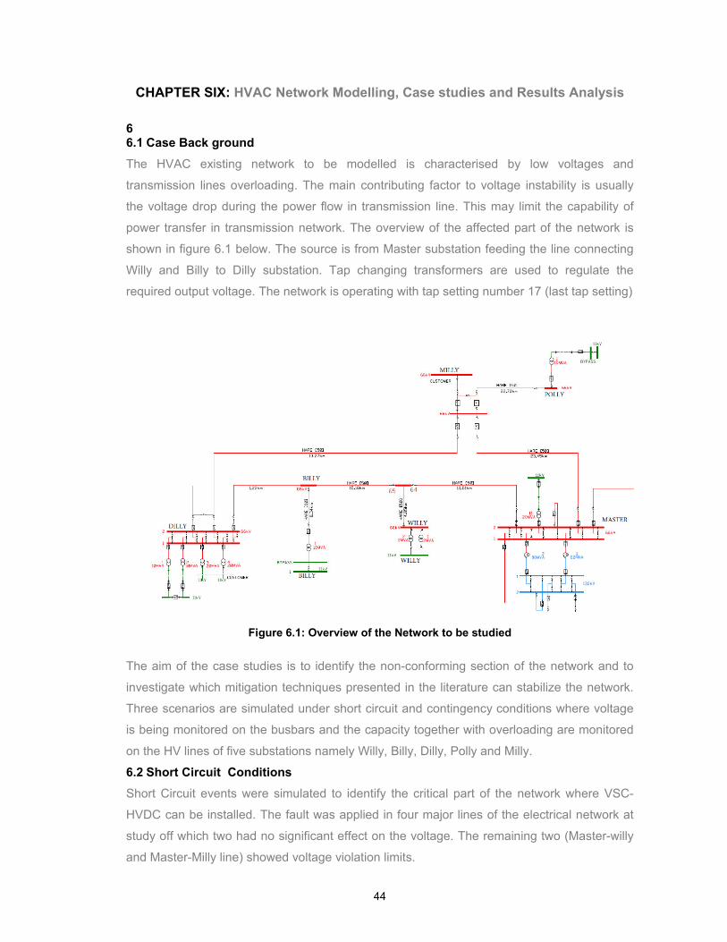
44
CHAPTER SIX: HVAC Network Modelling, Case studies and Results Analysis
6 6.1 Case Back ground
The HVAC existing network to be modelled is characterised by low voltages and
transmission lines overloading. The main contributing factor to voltage instability is usually
the voltage drop during the power flow in transmission line. This may limit the capability of
power transfer in transmission network. The overview of the affected part of the network is
shown in figure 6.1 below. The source is from Master substation feeding the line connecting
Willy and Billy to Dilly substation. Tap changing transformers are used to regulate the
required output voltage. The network is operating with tap setting number 17 (last tap setting)
Figure 6.1: Overview of the Network to be studied
The aim of the case studies is to identify the non-conforming section of the network and to
investigate which mitigation techniques presented in the literature can stabilize the network.
Three scenarios are simulated under short circuit and contingency conditions where voltage
is being monitored on the busbars and the capacity together with overloading are monitored
on the HV lines of five substations namely Willy, Billy, Dilly, Polly and Milly.
6.2 Short Circuit Conditions
Short Circuit events were simulated to identify the critical part of the network where VSC-
HVDC can be installed. The fault was applied in four major lines of the electrical network at
study off which two had no significant effect on the voltage. The remaining two (Master-willy
and Master-Milly line) showed voltage violation limits.

45
Figure 6.2: Master-willy fault clearing event
From figure 6.2 above, the blue thick line has been set as minimum operational constant of
0.925 per unit. Any busbar voltage that goes below this minimum set point is in violation of
voltage regulation standards. The fault was applied for two seconds and cleared. Out of
fifteen bubars being monitored, five busbars do not meet the minimum operational voltage of
0.925 per unit. This means that under fault conditions, thirty three percent of the customers
are adversely affected by fault occurrences.
2.0001.6001.2000.8000.4000.000 [s]
1.09
1.04
0.99
0.94
0.89
0.84
[p.u.]
Billy 11 BB1: Voltage, Magnitude
Billy 66 BB1: Voltage, Magnitude
Dilly 11 BB1: Voltage, Magnitude
Dilly 11 BB2: Voltage, MagnitudeD\Dilly 66 BB1: Voltage, Magnitude
Single Busbar\Master 132 BB1: Voltage, Magnitude
Single Busbar(1)\Master 66 BB2: Voltage, Magnitude
Master BB11: Voltage, Magnitude
Milly 6.6 BB1: Voltage, Magnitude
Single Busbar(4)\Milly 66 BB1: Voltage, Magnitude
Pilly 66 BB1: Voltage, Magnitude
Polly 11BB1: Voltage, Magnitude
Polly 66_1: Voltage, Magnitude
Willy 11 BB1: Voltage, Magnitude
Willy 66 BB1: Voltage, Magnitude
Master-Willy fault clearing event
Y =
0.9
25
p.u
.
0.000 s 0.204 s

46
Figure 6.3: Master-willy open switch event
Figure 6.3 above shows an event where a fault occurred at Master –Willy overhead line and
the switch remained open. It can be seen that seventy three percent of the network cannot
deliver power to the customers as the bus voltages are below the minimum operating point of
0.925 per unit. If one takes a closer look on the colour coding of the busbars, it is mostly
Masters Substation busbars (the source) that meets voltage regulation standards beyond
minimum operational level.
The same principle was applied on master-Milly overhead line where a fault clearing and
open switch events were monitored. Figure 6.4 and 6.5 show the results of such events. The
network behaviour is more or less the same as that of Master-Willy events.
2.0001.6001.2000.8000.4000.000 [s]
1.10
1.00
0.90
0.80
0.70
0.60
[p.u.]
Billy 11 BB1: Voltage, Magnitude
Billy 66 BB1: Voltage, Magnitude
Dilly 11 BB1: Voltage, Magnitude
Dilly 11 BB2: Voltage, MagnitudeD\Dilly 66 BB1: Voltage, Magnitude
Single Busbar\Master 132 BB1: Voltage, Magnitude
Single Busbar(1)\Master 66 BB2: Voltage, Magnitude
Master BB11: Voltage, Magnitude
Milly 6.6 BB1: Voltage, Magnitude
Single Busbar(4)\Milly 66 BB1: Voltage, Magnitude
Pilly 66 BB1: Voltage, Magnitude
Polly 11BB1: Voltage, Magnitude
Polly 66_1: Voltage, Magnitude
Willy 11 BB1: Voltage, Magnitude
Willy 66 BB1: Voltage, Magnitude
Master-Willy open switch event
Y =
0.9
25
p.u
.
0.000 s 0.204 s

47
Figure 6.4: Master-Milly fault clearing event
Figure 6.5: Master-Milly open switch event
2.0001.6001.2000.8000.4000.000 [s]
1.09
1.04
0.99
0.94
0.89
0.84
[p.u.]
Billy 11 BB1: Voltage, Magnitude
Billy 66 BB1: Voltage, Magnitude
Dilly 11 BB1: Voltage, Magnitude
Dilly 11 BB2: Voltage, MagnitudeD\Dilly 66 BB1: Voltage, Magnitude
Single Busbar\Master 132 BB1: Voltage, Magnitude
Single Busbar(1)\Master 66 BB2: Voltage, Magnitude
Master BB11: Voltage, Magnitude
Milly 6.6 BB1: Voltage, Magnitude
Single Busbar(4)\Milly 66 BB1: Voltage, Magnitude
Pilly 66 BB1: Voltage, Magnitude
Polly 11BB1: Voltage, Magnitude
Polly 66_1: Voltage, Magnitude
Willy 11 BB1: Voltage, Magnitude
Willy 66 BB1: Voltage, Magnitude
Master-Milly fault clearing event
Y =
0.9
25
p.u
.
0.000 s 0.204 s
2.0001.6001.2000.8000.4000.000 [s]
1.10
1.00
0.90
0.80
0.70
0.60
[p.u.]
Billy 11 BB1: Voltage, Magnitude
Billy 66 BB1: Voltage, Magnitude
Dilly 11 BB1: Voltage, Magnitude
Dilly 11 BB2: Voltage, MagnitudeD\Dilly 66 BB1: Voltage, Magnitude
Single Busbar\Master 132 BB1: Voltage, Magnitude
Single Busbar(1)\Master 66 BB2: Voltage, Magnitude
Master BB11: Voltage, Magnitude
Milly 6.6 BB1: Voltage, Magnitude
Single Busbar(4)\Milly 66 BB1: Voltage, Magnitude
Pilly 66 BB1: Voltage, Magnitude
Polly 11BB1: Voltage, Magnitude
Polly 66_1: Voltage, Magnitude
Willy 11 BB1: Voltage, Magnitude
Willy 66 BB1: Voltage, Magnitude
Master-Milly open switch event
Y =
0.9
25
p.u
.
0.000 s 0.204 s

48
6.3 Contingency Conditions
An emergency restoration plan was set out in order to manage the network during
emergency conditions and minimise the supply interruption time. The network at study was
monitored under three scenarios namely normal operation, N-1 with loss of Master-Willy
66kV overhead power line and N-1 with loss of Master-Milly 66kV overhead power line. Of
the three scenarios, busbar voltage, percentage loading of the line as well as power carrying
capacity in megawatts were monitored.
6.3.1 The normal operation network problem scenario 1 Simulation were done, the calculations converges. However the network does not deliver the
required voltage in some of the substations on the interconnected power system. Zooming in
onto figure 6.6 below, the 66kV busbar voltage at Dilly substation is 0.91 per unit. This value
is below the minimum requirement of 0.925 per unit as set out on voltage apportionment
limits for HV networks. It must be borne in mind that this is a load substation hence the
prohibition of adding new loads to this network. On the other hand the backbone
transmission lines are overloading close to 100% capacity and beyond while the maximum
power transfer capacity is only 31 megawatts, see figure 6.7 and 6.8. This network behaviour
raises voltage stability concerns as outlined in chapter five of this thesis.
Figure 6.6: Busbar voltage normal operation
BB
Bill
y 11
BB
1
Bill
y 66
BB
1
Dill
y 11
BB
1
Dill
y 11
BB
2
Dill
y 66
BB
1
Dill
y 66
BB
2M
aste
r 132
BB
1M
aste
r 66
BB
2
Mas
ter B
B11
Mill
y 6.
6 B
B1
Mill
y 66
BB
1
Pill
y 66
BB
1
Pol
ly 1
1BB
1
Pol
ly 6
6_1
Will
y 11
BB
1
Will
y 66
BB
1
1.50
1.20
0.90
0.60
0.30
0.00
Voltage, Magnitude in p.u.
Normal Operation Busbar voltage
[p.u]
Busbar

49
Figure 6.7: Normal Operation % Overheadline Loading
Figure 6.8: Line capacity normal operation
Bill
y-P
illy
66
Dill
y-M
illy
66_1
Dill
y-P
illy
66_
Line
Line
Mas
ter-
Mill
y 66
_ Li
ne
Mas
ter-
Will
y lin
k 66
_1
Mill
y-P
olly
66_
1
P-W
-L 6
6
Will
iy-W
illy
Link
66_
1
150.00
120.00
90.00
60.00
30.00
0.00
Loading in %
Normal Operation % Overheadline Loading
Overhead lines
[%L]
110 .437
105 .771
Bill
y-P
illy
66
Dill
y-M
illy
66_1
Dill
y-P
illy
66_
Line
Line
Mas
ter-
Mill
y 66
_ Li
ne
Mas
ter-
Will
y lin
k 66
_1
Mill
y-P
olly
66_
1
P-W
-L 6
6
Will
iy-W
illy
Link
66_
1
60.00
40.00
20.00
-20.00
-40.00
0.000
Active Power in MW
Capacity in MW Normal Operation
[MW]
31 .65
27 .30
Overheadlines
-15.75

50
6.3.2 The Master-Willy leg off network problem scenario 2 If Master-Willy 66kV line is out of service, Willy, Billy and Dilly 66kV busbars voltage drops to
minimum of 0.8 p.u respectively. This implies that under no circumstances will this line be out
of service. On the other hand, the Master-Milly 66kV line get to be overloaded to 187% of
Rate A rating and 102% of rate B rating of the conductor. Therefore Willy substation cannot
be supplied due to low voltages and overloading (Thermal limits).Under this scenario three
isolation points were opened along the line so as to verify this drastic voltage drop. Figure
6.9, 6.10 and 6.11 below shows the measured values at all affected busbars with their
respective % line loading and power values.
Figure 6.9: N-1 Master-Willy Busbar Voltage
BB
Bill
y 11
BB
1
Bill
y 66
BB
1
Dill
y 11
BB
1
Dill
y 11
BB
2
Dill
y 66
BB
1
Dill
y 66
BB
2M
aste
r 132
BB
1M
aste
r 66
BB
2
Mas
ter B
B11
Mill
y 6.
6 B
B1
Mill
y 66
BB
1
Pill
y 66
BB
1
Pol
ly 1
1BB
1
Pol
ly 6
6_1
Will
y 11
BB
1
Will
y 66
BB
1
1.50
1.20
0.90
0.60
0.30
0.00
Voltage, Magnitude in p.u.
N-1 Scenario 2 Busbar voltage
[p.u]
Busbar

51
Figure 6.10: N-1 Master-Willy % Overhead line loading
Figure 6.11: Line capacity N-1 Master-Willy
Bill
y-P
illy
66
Dill
y-M
illy
66_1
Dill
y-P
illy
66_
Line
Line
Mas
ter-
Mill
y 66
_ Li
ne
Mas
ter-
Will
y lin
k 66
_1
Mill
y-P
olly
66_
1
P-W
-L 6
6
Will
iy-W
illy
Link
66_
1
200.00
160.00
120.00
80.00
40.00
0.00
Loading in %
N-1 Master Willy % Overheadline Loading
Overhead lines
[%L]
187 .147
143 .215
Bill
y-P
illy
66
Dill
y-M
illy
66_1
Dill
y-P
illy
66_
Line
Line
Mas
ter-
Mill
y 66
_ Li
ne
Mas
ter-
Will
y lin
k 66
_1
Mill
y-P
olly
66_
1
P-W
-L 6
6
Will
iy-W
illy
Link
66_
1
60.00
40.00
20.00
-20.00
-40.00
0.000
Active Power in MW
Capacity in MW N-1 Scenario 2
[MW] 51 .58
34.55
Overheadlines
-8.797

52
6.3.3 The Master-Milly leg off network problem scenario 3 If Master –Milly 66kV line is out of service, Willy 66kV busbar voltage drops to 0.93 pu. Billy
and Dilly 66kV busbar voltage drops to 0.82 p.u respectively. Milly busbar voltage drops to
0.81 followed by Polly, the most severely affected busbar at 0.78 p.u. On the other hand, the
Master-willy 66kV line get to be overloaded to 45MVA at 193.83% of Rate A rating and 100%
of rate B rating of the conductor. Therefore Billy cannot be supplied due to low voltages and
overloading (Thermal limits). Figure 6.12, 6.13 and 6.14 below shows the measured values
at all affected busbars with their respective % line loading and power values.
Figure 6.12: N-1 Master-Milly Scenario 3 busbar voltage
BB
Bill
y 11
BB
1
Bill
y 66
BB
1
Dill
y 11
BB
1
Dill
y 11
BB
2
Dill
y 66
BB
1
Dill
y 66
BB
2M
aste
r 132
BB
1M
aste
r 66
BB
2
Mas
ter B
B11
Mill
y 6.
6 B
B1
Mill
y 66
BB
1
Pill
y 66
BB
1
Pol
ly 1
1BB
1
Pol
ly 6
6_1
Will
y 11
BB
1
Will
y 66
BB
1
1.50
1.20
0.90
0.60
0.30
0.00
Voltage, Magnitude in p.u.
N-1 Scenario 3 Busbar voltage
[p.u]
Busbar

53
Figure 6.13: N-1 Master-Milly % Overhead line loading
Figure 6.14: Line capacity N-1 Master-Milly
Bill
y-P
illy
66
Dill
y-M
illy
66_1
Dill
y-P
illy
66_
Line
Line
Mas
ter-
Mill
y 66
_ Li
ne
Mas
ter-
Will
y lin
k 66
_1
Mill
y-P
olly
66_
1
P-W
-L 6
6
Will
iy-W
illy
Link
66_
1
250.00
200.00
150.00
100.00
50.00
0.00
Loading in %
N-1 Master Milly % Overheadline Loading
Overhead lines
[%L]
189 .413193 .836
Bill
y-P
illy
66
Dill
y-M
illy
66_1
Dill
y-P
illy
66_
Line
Line
Mas
ter-
Mill
y 66
_ Li
ne
Mas
ter-
Will
y lin
k 66
_1
Mill
y-P
olly
66_
1
P-W
-L 6
6
Will
iy-W
illy
Link
66_
1
60.00
40.00
20.00
-20.00
-40.00
0.000
Active Power in MW
Capacity in MW N-1 Scenario 3
[MW]
53.87
48 .88
Overheadlines
-9.75

54
6.4 Analysis of results
The results recoded in figures 6.2-6.14 are for voltage magnitude in per unit, percentage
loading of the backbone overhead transmission lines and power carrying capacity when
Existing AC network is subjected to disturbances of various types and magnitudes .HV
Network abnormalities affects a bigger number of consumers and therefore maintenance
needs to be preventative and condition based. The power system security is a worrying
factor as the network cannot withstand the effects of contingency and short circuit
disturbances. This system is operated in heavily stressed conditions and is becoming more
complicated to manage. According to Eskom distribution voltage and apportionment limits
standard (DST_34-542) the recommended sub-transmission HV limits to be used are listed
in figure 6.15 below. It can be seen from figures 6.2-6.14 that this portion of the network
barely conforms to the minimum operating voltage as set out in HV standards in figure 6.15.
Figure 6.15: Standard operating Voltage limits for HV network
Looking at the ‘normal operation network” results, the operation is under severely stressed
condition. Voltages of the system are partly below the accepted range; low voltage
transformers as well as overhead transmission lines are showing the signs of being
overloaded .furthermore there are no guarantees that the system can maintain stability
during disturbances because the power system planning design is no longer compatible to
today’s electricity demand.
The “Master-Willy leg off” results shows the system has been weakened to a level where a
contingency violates the voltage regulation limits.as per figure 6.15, the minimum voltage is
88.5% provided that there are no HV customers and MV regulation is adequate.in all five
substations the HV busbar is below the minimum limit.at this state the system transits into
emergency state where control actions need to be applied to restore the system back to
normal state. More or less the same behaviour was observed when master-Milly leg was out
of service and therefore the third scenario will not be further elaborated.

55
Figure 6.16 shows the voltage profile of HV network under peak loading conditions. The
sending end voltage is controlled by on-load tap changer transformer situated at Master
substation. The transformer has reached the last tap setting and therefore no compensation
method can be further applied by the component. From the planning perspective the
operational voltage should be any value between 95% and 105% as shown in figure 6.15.
However for operational purposes which are inclusive of contingency simulation studies
allows the minimum of 92, 5% and maximum of 107, 5 % of abnormal voltage. It can be seen
that the voltage decreases with distance away from source substation, which should be the
case on distribution feeder. However it must range within allowable limits, which is not the
case with figure 6.16.the voltage regulations limits are way violated. Also the red colour
shows the overloaded transmission line thus another limiting factor on the capacity of the
line.
Figure 6.16: Voltage Profile
From the base case scenarios, 66kV bursars reactive power was also monitored.at Willy and
Billy substations, a very small change that is an increase in reactive power is observed when
the volt drop of 15% occurs. This is more evident at Dilly substation, where a significant
change in voltage causes a noticeable change in reactive power. Under normal operation the
reactive power is 5.99 MVARs. Under case B the voltage drops about 14% and the
corresponding reactive power is 9.35MVARs. This implies that Dilly is a load substation and
any rise in reactive power causes undesirable voltage drops and thermal loading.

56
It can be observed that the existing AC network is facing problem of low supply voltage tied
with shortage of electrical energy. This is due to utilization of low current carrying capacity
conductors that are overloaded and ultimately lead to volt drop and energy/power loses. This
used to be a low voltage distribution network problem. However developing countries are
faced with financial problems which prohibit them from upgrading the existing HV networks.
Network development plans would be focused on assessing the network requirements to
meet additional loads and address issues that cannot be solved by optimisation of the
existing network ensure that Distribution networks meet the minimum quality of supply,
reliability and operational requirements as specified in the Distribution Network Code. The
focus should be on improving power quality on constrained networks first, then reliability.

57
CHAPTER SEVEN: VSC-HVDC network modelling 7 7.1 Guideline for incorporating VSC-HVDC link in to weak AC system
This section details the power system analysis guideline followed in this thesis. The flow
chart in figure 7.1 shows the outlined procedure followed when incorporating VSC-based
HVDC link on the base case network studied in chapter 6. This is a high level procedure
adopted by utilities. The VSC-HVDC system capabilities will be applied to see if there is a
need for any network upgrade. Furthermore, is there any network capacity enhancement
realized.
Figure 7.1: Flow diagram for VSC-HVDC link incorporation procedure (DNOP_240-82534300)

58
7.2 Modelling of a VSC-HVDC link
Figure 7.2 shows the single line diagram of a VSC-HVDC link as modelled on Digsilent
power factory. For the purpose of this study, a simplified modelling approach was adopted
where two converters are connected to one another by the HVDC transmission line. This
VSC grid model is a replacement of existing HVAC link. The maximum increase in power
transfer capability and voltage control will be based on a simplified transmission line model
for short transmission lines.
Figure 7.2: VSC-HVDC link single line diagram
Power factory network reduction tool was used to provide a simplified representation of the
AC network that contains the interface points. The two connection nodes are 132kV busbar
with blue colour coding and 66kV busbar with red colour coding. The two converters were
modelled as voltage source converters where an offs-sure converter was connected at 132
kV busbar on the source side of AC the network (see figure 7.4 rated AC-voltage).An on-sure
converter was connected to 66kV busbar on the load side of the AC network (see figure 7.5
rated AC-voltage).
This type of arrangement also proves the phenomena highlighted by ( Andersen , 2013:4) in
chapter three of this thesis where he mentions that VSC-technology is not only limited to long
distance transmission. Secondly it can be observe that it fulfils a situation where HVDC
systems can be applied and expanded in a manner similar to AC substations. Initial step of
the adopted flow chart presented in figure 7.1 is implemented at this stage of the simulation
procedure. Standard network check and load flow studies were successfully executed.

59
7.3 Fault level assessment after VSC-HVDC link incorporation
Following the steps as set out on the guideline and using the reduced network representation
in figure 7.2, the fault level assessment was carried out in a form of short circuit analysis to
ascertain the system’s adequate handling of short circuit. The outcome of the fault
assessment may be to change the VSC-HVDC link control set-points or network
configuration as the goal is to isolate the short circuit safely with minimal damage on the
equipment and system interruption.
Recalling the short circuit results that failed the short circuit test in chapter 6, it was
imperative to conduct the short circuit analysis so as to verify the admissible thermal limits of
transmission lines and voltage tolerance of the system. Figure 7.3 is a demonstration of how
the study could be simulated on power factory. It was then identified that the suitable position
for VSC-HVDC link is between Master and Dilly substations.
Figure 1.3: Fault level assessment
7.4 Determination of VSC-HVDC control modes
It has been mentioned on the literature review in chapter three section 3.8 that VSC-HVDC
has got the capability to control the system. Different control strategies were highlighted but
the most documented one is a vector current control system, as a consequence the vector
current control has been used on this thesis. The following basic data shown in Figure 7.4
and 7.5 was entered for the off-sure and on-sure converters respectively.
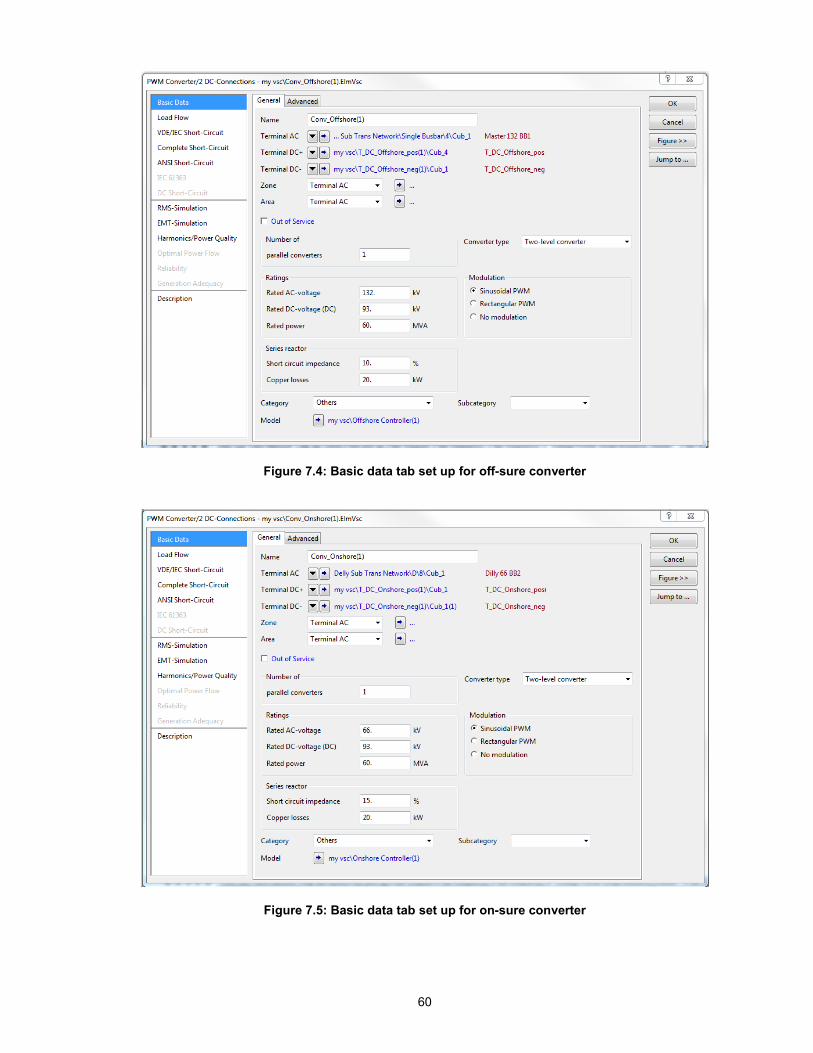
60
Figure 7.4: Basic data tab set up for off-sure converter
Figure 7.5: Basic data tab set up for on-sure converter

61
The voltage source converters come with station controller where a set point needs to be
selected according the desired needs of the intended operation. Here a voltage control,
power factor control and reactive power control mode can be chosen.in figure 7.6 below, P-Q
control mode was selected for an off-sure converter to control the power of the system at
study.
Figure 7.6: Power control mode
Therefore, on the on-sure converter the Vdc-Q mode was selected, this where the DC voltage is being controlled as the conversion from DC-to-AC takes place.
Figure 7.7: DC voltage control mode

62
CHAPTER EIGHT: Results, Discussion and Recommendations 8 8.1 Short circuit conditions after Integration of VSC-HVDC link
After following methodology described in Chapter seven and subjecting the network to
operation scenarios described in chapter six with VSC-HVDC link incorporated to the system,
a variety of results were obtained. The VSC-HVDC link provided power enhancement
capabilities and voltage control. A large disturbance was introduced into the system in a
form of short circuit to both Willy and Milly 66kV overhead lines. Typically such faults are
meant to depress the system voltage, cause synchronous generators to speed up and cause
non-synchronous generators to enter FRT mode. Figure 8.1 and 8.2 show the results of the
fault occurrence after it was cleared after 200ms.from both figures it can be observed that the
minimum bus voltage is 0.972 pu. This is way above the blue thick line that has been set as
minimum operational constant of 0.925 per unit. The VSC incorporation to the system
improved the system security, quality, stability, reliability and availability thereby keeping bus
voltages within acceptable limits even after a fault.
Figure 2.1: Master-willy VSC fault clearing event
2.001.601.200.800.400.00 [s]
1.09
1.04
0.99
0.94
0.89
0.84
[p.u.]
Billy 11 BB1: Voltage, Magnitude
Billy 66 BB1: Voltage, Magnitude
Dilly 11 BB1: Voltage, Magnitude
Dilly 11 BB2: Voltage, Magnitude
D\Dilly 66 BB1: Voltage, MagnitudeSingle Busbar\Master 132 BB1: Voltage, Magnitude
Single Busbar(1)\Master 66 BB2: Voltage, Magnitude
Master BB11: Voltage, Magnitude
Milly 6.6 BB1: Voltage, Magnitude
Single Busbar(4)\Milly 66 BB1: Voltage, Magnitude
Pilly 66 BB1: Voltage, Magnitude
Polly 11BB1: Voltage, Magnitude
Polly 66_1: Voltage, Magnitude
Willy 11 BB1: Voltage, Magnitude
Willy 66 BB1: Voltage, Magnitude
Master-Willy VSC fault clearing event
Y =
0.
925
p.u.
0.000 s 0.206 s
1.301 s 0.972 p.u.
1.651 s 1.064 p.u.

63
Figure 8.2: Master-Milly VSC fault clearing event
The same network was subjected to a large disturbance and the switch remained open. Once a breaker starts tripping, it easier to reach voltage violation because the system becomes weaker. However from figures 8.3 and 8.4, it can be observed that the minimum bus voltage is 0.972 pu and 0.954 pu respectively. The VSC incorporation improved network low voltages above the minimum acceptable operating voltage of 0.925 pu. None of the busbars are reaching voltage violation therefore. The results of this study clearly show the VSC-HVDC link capability to autonomously modify its active and reactive power output into the distribution and sub-transmission system in response to changes in voltage that was presented on chapter six figures 6.3 and 6.5 respectively.
2.001.601.200.800.400.00 [s]
1.09
1.04
0.99
0.94
0.89
0.84
[p.u.]
Billy 11 BB1: Voltage, Magnitude
Billy 66 BB1: Voltage, Magnitude
Dilly 11 BB1: Voltage, Magnitude
Dilly 11 BB2: Voltage, Magnitude
D\Dilly 66 BB1: Voltage, MagnitudeSingle Busbar\Master 132 BB1: Voltage, Magnitude
Single Busbar(1)\Master 66 BB2: Voltage, Magnitude
Master BB11: Voltage, Magnitude
Milly 6.6 BB1: Voltage, Magnitude
Single Busbar(4)\Milly 66 BB1: Voltage, Magnitude
Pilly 66 BB1: Voltage, Magnitude
Polly 11BB1: Voltage, Magnitude
Polly 66_1: Voltage, Magnitude
Willy 11 BB1: Voltage, Magnitude
Willy 66 BB1: Voltage, Magnitude
Master-Milly VSC fault clearing event
Y =
0.
925
p.u.
0.000 s 0.205 s
1.072 s 0.972 p.u.
1.732 s 1.064 p.u.

64
Figure 8.3: Master-Willy VSC open switch event
Figure 8.4: Master-Milly VSC open switch event
2.001.601.200.800.400.00 [s]
1.10
1.05
1.00
0.95
0.90
0.85
[p.u.]
Billy 11 BB1: Voltage, Magnitude
Billy 66 BB1: Voltage, Magnitude
Dilly 11 BB1: Voltage, Magnitude
Dilly 11 BB2: Voltage, Magnitude
D\Dilly 66 BB1: Voltage, MagnitudeSingle Busbar\Master 132 BB1: Voltage, Magnitude
Single Busbar(1)\Master 66 BB2: Voltage, Magnitude
Master BB11: Voltage, Magnitude
Milly 6.6 BB1: Voltage, Magnitude
Single Busbar(4)\Milly 66 BB1: Voltage, Magnitude
Pilly 66 BB1: Voltage, Magnitude
Polly 11BB1: Voltage, Magnitude
Polly 66_1: Voltage, Magnitude
Willy 11 BB1: Voltage, Magnitude
Willy 66 BB1: Voltage, Magnitude
Master-Willy VSC open switch event
Y =
0.
925
p.u.
0.000 s 0.206 s
0.944 s 0.975 p.u.
1.324 s 1.064 p.u.
2.001.601.200.800.400.00 [s]
1.10
1.05
1.00
0.95
0.90
0.85
[p.u.]
Billy 11 BB1: Voltage, Magnitude
Billy 66 BB1: Voltage, Magnitude
Dilly 11 BB1: Voltage, Magnitude
Dilly 11 BB2: Voltage, Magnitude
D\Dilly 66 BB1: Voltage, MagnitudeSingle Busbar\Master 132 BB1: Voltage, Magnitude
Single Busbar(1)\Master 66 BB2: Voltage, Magnitude
Master BB11: Voltage, Magnitude
Milly 6.6 BB1: Voltage, Magnitude
Single Busbar(4)\Milly 66 BB1: Voltage, Magnitude
Pilly 66 BB1: Voltage, Magnitude
Polly 11BB1: Voltage, Magnitude
Polly 66_1: Voltage, Magnitude
Willy 11 BB1: Voltage, Magnitude
Willy 66 BB1: Voltage, Magnitude
Master-Milly VSC open switch event
Y =
0.
925
p.u.
0.000 s 0.205 s 0.266 s 0.729 s
1.257 s 0.954 p.u.
1.667 s 1.064 p.u.

65
8.2 Contingency conditions after Integration of VSC-HVDC link
8.2.1 The normal operation network problem scenario 1 The normal operating conditions that are considered are the busbar voltages (above 95%)
and the line loadings (below 100% at rate A) that complement the power carrying capacity of
the main lines. The normal operation network problem scenario had to be looked at in the
abnormal need set or contingency conditions due to the fact that it previously violated the
voltage and loading limits. What was deemed as normal was abnormal so it can be assumed
that if there was no need under normal operating conditions, no further normal condition
studies need to be looked at. The VSC-HVDC link that was imbedded inside the AC network
was used to strengthen the weak points of the power system at the same time increase
power transmission capacity of the network. The attention is given to busbar voltages of the
affected network (figure 8.1), percentage loading of the two overhead transmission lines
being Milly and Willy 66kV (figure 8.2) as well as power carrying capacity of these two lines
(figure 8.3) .referencing back to chapter 6 figure 6.6, we could see a minimum voltage of 0.91
pu. However with VSC incorporation, the minimum busbar voltage of 0.99 pu at Polly 66_1 is
observed. This shows a remarkable improvement as the voltage is almost 1 pu. Voltage
stability is said to be the one of the limiting factors for power transfer in the transmission grid.
However Simulations studies shows that even with small VSC-HVDC transmission capacity,
VSC-HVDC links can significantly improve voltage stability.
Figure 8.1: VSC Busbar voltage normal operation
BB
Bill
y 11
BB
1
Bill
y 66
BB
1
Dill
y 11
BB
1
Dill
y 11
BB
2
Dill
y 66
BB
1
Dill
y 66
BB
2M
aste
r 132
BB
1M
aste
r 66
BB
2
Mas
ter B
B11
Mill
y 6.
6 B
B1
Mill
y 66
BB
1
Pill
y 66
BB
1
Pol
ly 1
1BB
1
Pol
ly 6
6_1
Will
y 11
BB
1
Will
y 66
BB
1
1.25
1.00
0.75
0.50
0.25
0.00
Voltage, Magnitude in p.u.
VSC Normal Operation Busbar voltage
[p.u]
Busbar
0.99

66
Ideally these transmission lines are set to operate at 80% maximum specified loading limit
under normal network status. Anything above this rate calls for contingency intervention.
Depicted from figure 8.2 percentage line loading for Master-Milly and Master- Willy 66 KV
lines are now 38% and 42% respectively. A huge improvement can be witnessed as the lines
were previously overloaded at 98% and 110 %. It must be borne in mind that these values
are of the same voltage level, same network load and same probabilistic ampacity values.
The very same Hare conductor @ 50 degrees template; rated 32 MVA under normal and 45
MVA under emergency was used. Thermal Loading problems and Voltage limits Violations
(Normal Conditions)
Normal ratings (Rate A) of the conductors were used for Normal Network Status.
Figure 8.2: VSC Normal Operation % Overheadline Loading
According to ABB, the number of HVDC links in AC systems result in a more controllable and
precise power exchange. As can be seen from figure below, The HVDC link was used to
control power flow in a weak AC network. Under normal operation, Master-Milly and Master-
Willy 66 KV lines were delivering 27.3 and 31.65 MW of power respectively. After VSC-
HVDC link it can be observed that the two lines are now delivering 3.67 and 0.488 MW of
power respectively. There is a difference of 23 and 31.16 MW meaning the power carrying
capacity has been enhanced and optimised through the existing lines, both lines can still
push more power at the same voltage level. DC can transmit 2-to-3 times more power
without any stability problems
Bill
y-P
illy
66
Dill
y-M
illy
66_1
Dill
y-P
illy
66_
Line
Line
Mas
ter-
Mill
y 66
_ Li
ne
Mas
ter-
Will
y lin
k 66
_1
Mill
y-P
olly
66_
1
P-W
-L 6
6
Will
iy-W
illy
Link
66_
1
150.00
120.00
90.00
60.00
30.00
0.00
Loading in %
VSC Normal Operation % Line Loading
Overhead lines
[%L]
42.8938.97

67
Figure 8.3: VSC Line capacity normal operation
8.2.2 The Master-Willy leg off network problem scenario 2
Abnormal conditions put a lot more stress on the network, as the allowable line loading is
increased (100% at rate A to 100% at rate B) and the minimum busbar voltage decreases
(95% to 92.5%). As the relationships between these standard limitations are not linear,
several needs are expected to arise in the event that an asset performs near the allowable
threshold. Abnormal conditions also contain a multitude of different combinations, focusing
mainly on Master-Milly 66kV line and the network busbar voltages.
Given that the Master-Willy line failed the contingency analysis to a point where the minimum
voltage was 0.8 pu or 80% and the line loading of Master-Milly was 187% at rate-B.The
busbar voltage results presented on figure 8.4 show a tremendous improvement as the
minimum bus voltage is 0.97 pu or 97 % at Billy 66kV busbar under N-1 conditions. A greater
increase of 4.25% above the minimum allowable voltage of 92.5% is observed. This in turn
shows a firm and reliable network under N-1 conditions.
Bill
y-P
illy
66
Dill
y-M
illy
66_1
Dill
y-P
illy
66_
Line
Line
Mas
ter-
Mill
y 66
_ Li
ne
Mas
ter-
Will
y lin
k 66
_1
Mill
y-P
olly
66_
1
P-W
-L 6
6
Will
iy-W
illy
Link
66_
1
60.00
40.00
20.00
-20.00
-40.00
0.000
Active Power in MW
Capacity in MW VSC Normal Operation
[MW]
Overheadlines
0.488
3.677

68
Figure8.4: VSC N-1 Master-Willy Busbar Voltage
As there were both high line loadings and low voltage issues post VSC-HVDC link
incorporation, the solution proposed aught to address both of these need scenarios. Apart
from low voltage alleviation presented in figure 8.4, it is clear from figure 8.5 and 8.6 below
that the VSC incorporation improved the capacity of the lines. Under N-1 condition, the
Master-Milly 66kV line loading drops from 187.147% rate-B to 80.1% rate-A of the conductor
while there is a spare capacity of 50MW that could be delivered in case of any additional
load. VSC-HVDC brought a holistic solution that mitigates all contingency load and voltage
violations under N-1 conditions.
This implies that the station is very close to becoming overloaded, and it will be extremely
difficult to switch out a transformer to perform maintenance work
BB
Bill
y 11
BB
1
Bill
y 66
BB
1
Dill
y 11
BB
1
Dill
y 11
BB
2
Dill
y 66
BB
1
Dill
y 66
BB
2M
aste
r 132
BB
1M
aste
r 66
BB
2
Mas
ter B
B11
Mill
y 6.
6 B
B1
Mill
y 66
BB
1
Pill
y 66
BB
1
Pol
ly 1
1BB
1
Pol
ly 6
6_1
Will
y 11
BB
1
Will
y 66
BB
1
1.25
1.00
0.75
0.50
0.25
0.00
Voltage, Magnitude in p.u.
VSC N-1 Scenario 2 Busbar voltage
[p.u]
Busbar
0.97

69
Figure 8.5: VSC N-1 Master-Willy % Overhead line loading
Figure 8.6: VSC Line capacity N-1 Master-Willy
Bill
y-P
illy
66
Dill
y-M
illy
66_1
Dill
y-P
illy
66_
Line
Line
Mas
ter-
Mill
y 66
_ Li
ne
Mas
ter-
Will
y lin
k 66
_1
Mill
y-P
olly
66_
1
P-W
-L 6
6
Will
iy-W
illy
Link
66_
1
150.00
120.00
90.00
60.00
30.00
0.00
Loading in %
VSC N-1 Master Willy % Line Loading
Overhead lines
[%L]
0.49
80 .1
Bill
y-P
illy
66
Dill
y-M
illy
66_1
Dill
y-P
illy
66_
Line
Line
Mas
ter-
Mill
y 66
_ Li
ne
Mas
ter-
Will
y lin
k 66
_1
Mill
y-P
olly
66_
1
P-W
-L 6
6
Will
iy-W
illy
Link
66_
1
60.00
40.00
20.00
-20.00
-40.00
0.000
Active Power in MW
VSC Capacity in MW N-1 Scenario 2
[MW]
Overheadlines
1.005

70
8.2.3 The Master-Milly leg off network problem scenario 3
According to Eskom Standard, (firm substations), distribution substations must be firm at all
times. This implies that in the event that a line or transformer is lost, the remaining lines or
transformers must be able to carry the entire load without operating past 100%.Due to the
configuration of the network at study, The N-1 contingency scenario had to be simulated
twice to fulfil the firm substation requirements. From figure 8.7 it can be deduced that the
substations busbar voltages improved substantially with the introduction of a VSC-HVDC
link. The minimum bus voltage is 0.95 pu or 95% at Polly substation. It should be noted that
this is an N-1 contingency scenario (abnormal condition) meeting the requirements of a
normal operating condition.
Figure 8.7: VSC N-1 Scenario 3 Busbar Voltage
Furthermore the line loading at Master-Milly 66kV line drops from 193.836% rate-B to
78.9% rate-A of the conductor while there is a spare capacity of 52MW that could be
delivered in case of any additional load. The percentage line loading and the capacity in
megawatts results are both advocating for the capacity enhancement as the topic of this
thesis suggests. It can be seen from Figure 8.8 and 8.9 Simulations results that it was not
by a chance that the VSC-HVDC link enhanced the network capacity.it can be concluded
that the terminals of VSC can be considered as voltage source.
BB
Bill
y 11
BB
1
Bill
y 66
BB
1
Dill
y 11
BB
1
Dill
y 11
BB
2
Dill
y 66
BB
1
Dill
y 66
BB
2M
aste
r 132
BB
1M
aste
r 66
BB
2
Mas
ter B
B11
Mill
y 6.
6 B
B1
Mill
y 66
BB
1
Pill
y 66
BB
1
Pol
ly 1
1BB
1
Pol
ly 6
6_1
Will
y 11
BB
1
Will
y 66
BB
1
1.25
1.00
0.75
0.50
0.25
0.00
Voltage, Magnitude in p.u.
VSC N-1 Scenario 3 Busbar voltage
[p.u]
Busbar
0.95

71
Figure 8.8: VSC N-1 Master Milly % Line Loading
Figure 8.9: VSC N-1 Master Milly % Line Loading
Bill
y-P
illy
66
Dill
y-M
illy
66_1
Dill
y-P
illy
66_
Line
Line
Mas
ter-
Mill
y 66
_ Li
ne
Mas
ter-
Will
y lin
k 66
_1
Mill
y-P
olly
66_
1
P-W
-L 6
6
Will
iy-W
illy
Link
66_
1
150.00
120.00
90.00
60.00
30.00
0.00
Loading in %
VSC N-1 Master Milly % Line Loading
Overhead lines
[%L]
0.88
78 .9
Bill
y-P
illy
66
Dill
y-M
illy
66_1
Dill
y-P
illy
66_
Line
Line
Mas
ter-
Mill
y 66
_ Li
ne
Mas
ter-
Will
y lin
k 66
_1
Mill
y-P
olly
66_
1
P-W
-L 6
6
Will
iy-W
illy
Link
66_
1
60.00
40.00
20.00
-20.00
-40.00
0.000
Active Power in MW
VSC Capacity in MW N-1 Scenario 3
[MW]
Overheadlines
1.247

72
8.3 Conclusion and Recommendations
The main goal of the thesis was to enhance the network capacity through HVDC link.
However the network on which the studies were performed did not only present the
bottlenecks but low voltage problems as well. The motivation for grid expansion lead to
evaluation of possible enhancement methods on HVAC networks as opposed to HVDC
networks and thereafter, two study cases each with three operating scenarios were
developed and simulation were ran for HVAC and HVDC configurations. The first study case
was using the existing HVAC line and the second study case was converting the AC line into
DC and replacing the HVAC line with a point-to-point VSC-HVDC link.
Different operating points were considered with respect to voltage and loading violation limits
for peak loads and contingency or abnormal conditions to examine the technical economical
viable solution. From this thesis, it can be concluded that the reliability, stability and security
of the system is a critical issue especially when the system is heavily loaded. This statement
is supported by the results presented in chapter six where the performance of the power
system decreased with the size and complexity of the network. The literature has been
referring to the future which is now, where the loading of the existing power system has
increased, leading to bottlenecks and reliability problems. On HVAC networks, if power
should be transmitted through interconnected systems, transmission lines needs to be
supported along the corridor. With an attempted support, the loading and voltage violations
couldn’t be solved simultaneously.
As a consequence, the needed enhancement of the power system was done through VSC-
HVDC link. The proposed VSC-HVDC link was able to enhance the capacity of the network
by modulating the active and reactive power of the HVDC link. DC interconnection survived
the N-1 contingency scenarios and assisted on power supply restoration under short circuit
conditions. From this it can be deduced that the incorporation of VSC-HVDC link proved to
be effective and it can be used for power system stability enhancement as well.
As far as trends in high voltage transmission systems were concerned, Power enhancement
capacity through power electronics was anticipated to happen at transmission, sub-
transmission and distribution systems. The VSC-HVDC can clearly strengthen the grid and
improve the performance of the system at all levels.
8.4 Limitations and Future work
The limitation of the study was the challenge to model the VSC-HVDC on power factory.
Detailed VSC-HVDC models from manufactures where the control structures are elaborated
73
are not available.one can either use the black box models from ABB or the control structure
of a generic type from Digsilent Power Factory. There is a lack of documentation
corresponding to the model behaviour.
From an academic point of view, the modelling challenges experienced in this thesis present
an opportunity for researchers to embark on documenting the VSC-HVDC model behaviour
especially on how the controllers of these models are tuned. Furthermore this will eliminate
the challenges faced when connecting renewable energies at distribution level particularly in
South Africa as the electrical power sector aims at increasing the penetration of renewable
resources.
74
CHAPTER NINE: BIBLIOGRAPHY ABB, 2017. HVDC Light it’s time to connect. [Online] Available at: www.abb.com/hvdc. Adeuyi, O. D., Cheah-mane, M., Liang, J., Livermore, L. & Mu, Q. 2015. Preventing DC over-voltage in multi-terminal HVDC transmission. CSEE Journal of Power and Energy Systems, 1, 86-94. Agelidis, V. G., Demetriades, G. D. & Flourentzou, N. 2006. Recent advances in high-voltage direct-current power transmission systems. Alharbi, M. M. 2014. Modeling of multi-terminal VSC-based HVDC systems. Andersen, B. R. Cigre and trends in power electronics for the grid. 2013 15th European Conference on Power Electronics and Applications (EPE), 2013. IEEE, 1-8. Arifoglu, U. 2003. The power flow algorithm for balanced and unbalanced bipolar multiterminal ac–dc systems. Electric Power Systems Research, 64, 239-246. Arrillaga, J. & Arrillaga, J. 1998. High voltage direct current transmission, IET. Arrillaga, J., Liu, Y. H. & Watson, N. R. 2007. Flexible power transmission: the HVDC options, John Wiley & Sons. Assis, T. M. L., Kuenzel, S. & PAL, B. C. 2016. Impact of multi-terminal HVDC grids on enhancing dynamic power transfer capability. IEEE Transactions on Power Systems, 32, 2652-2662. Baradar, M. 2013. Modeling of multi terminal hvdc systems in power flow and optimal power flow formulations. KTH Royal Institute of Technology. Bayo salas, A. 2013. Operation, control and optimization of a Meshed-HVDC system. Universitat Politècnica de Catalunya. Behravesh, V. & Abbaspour, N. 2012. New Comparison of HVDC and HVAC Transmission system. International Journal of Engineering Innovation & Research, 1, 300-304. Bucher, M. A., Wiget, R., Pérez, G. H.-B. & Andersson, G. Optimal placement of multi-terminal HVDC interconnections for increased operational flexibility. IEEE PES Innovative Smart Grid Technologies, Europe, 2014. IEEE, 1-6. Clarke, A, 2002. Technical Aspects of Electrical Cables, Aberdare Cables DIgSILENT , 2017. Power Factory User Manual. Gomaringen, Germany. Du, C. 2007. VSC-HVDC for industrial power systems, Chalmers University of Technology. Elserougi, A., Massoud, A. M., Abdel-khalik, A. S. & Ahmed, S. 2016. Three-wire bipolar high-voltage direct current line using an existing single-circuit high-voltage alternating current line for integrating renewable energy sources in multiterminal DC networks. IET Renewable Power Generation, 10, 370-379. Eskom, 2015. Distribution network Operations Planning (DNOP)Standard_240-82534300. Eskom, 2014. Distribution Voltage and Apportionment Limits Standard (DST_34-542). Geetha, R., Deekshit, R. & Lal, G. 2015. Controllers for A VSCHVDC link connected to a

75
weak AC system. IOSR Journal of Electrical and Electronics Engineering, 10, 18-32. Guo, C., Liu, W. & Zhao, C. 2013. Research on the control method for voltage-current source hybrid-HVDC system. Science China Technological Sciences, 56, 2771-2777. Haddad, A., Haddad, M., Warne, D. & Warne, D. 2004. Advances in high voltage engineering, IET. Humpert, C. 2012. Long distance transmission systems for the future electricity supply – Analysis of possibilities and restrictions. Energy, 48, 278-283. IEEE Power& Energy. n.d. DC Power Transmission Mercury-Arc to Thyristor HVdc Valves.[online] available at http://magazine.ieee-pes.org/marchapril-2014/history-12/ Imhof, M. 2015. Voltage Source Converter Based HVDC-Modelling and Coordinated Control to Enhance Power System Stability. ETH Zurich. Kabiri, R., Holmes, D. & Mcgrath, B. DigSILENT Modelling of Power Electronic Converters for Distributed Generation Networks. Power Factory Users' Conference and Future Networks Technical Seminar, 2013. Kasangala, F. & Atkinson-hope, G. Electrical energy losses and costs evaluation of HVDC and UHVDC transmission lines. 2013 Proceedings of the 10th Industrial and Commercial Use of Energy Conference, 2013. IEEE, 1-7. Chan-Ki Kim, Vijay K. Sood, Gil-Soo Jang, Seong-Joo Lim, Seok-Jin Lee. 2009. HVDC Transmission: Power Conversion Applications in Power Systems, : John Wiley & Sons Kjørholt, Å. M. H. 2014. HVDC transmission using a bipolar configuration composed of an LCC and MMC: operating characteristics of Skagerrak 3 and Skagerrak 4. Institutt for elkraftteknikk. Kothari, D. P. & Nagrath, I. 2011. Modern power system analysis, Tata McGraw-Hill Education. Kundur, P., Balu, N. J. & Lauby, M. G. 1994. Power system stability and control, McGraw-hill New York. Kundur, P., Paserba, J. & Vitet, S. Overview on definition and classification of power system stability. CIGRE/IEEE PES International Symposium Quality and Security of Electric Power Delivery Systems, 2003. CIGRE/PES 2003., 2003. IEEE, 1-4. Larruskain, D., Zamora, I., Abarrategui, O., Iraolagoitia, A., Gutiérrez, M., Loroño, E. & DE LA Bodega, F. Power transmission capacity upgrade of overhead lines. International Conference on Renewable Energy and Power Quality (ICREPQ), 2006. Larruskain, D. M., Zamora, I., Abarrategui, O., Buigues, G., Valverde, V. & Iturregi, A. 2014. Adapting AC Lines to DC Grids for Large-Scale Renewable Power Transmission. AIMS Energy, 2, 385-398. Lennerhag, O. & Träff, V. 2013. Modelling of VSC-HVDC for slow dynamic studies. Master's in Power Engineering, Department of Energy and Environment, Chalmers University of Technology, Sweden. Luo, F. L. & Hong, Y. 2017. Renewable energy systems: advanced conversion technologies and applications, CRC press. Luo, F. L. & Ye, H. 2018. Essential Dc/Dc Converters, CRC Press.

76
M'builu-ives, S. 2016. Stability Enhancement of HVAC Grids Using HVDC Links. University of KwaZulu-Natal, Pietermaritzburg. Machowski, J., Bialek, J. & Bumby, J. 2011. Power system dynamics: stability and control, John Wiley & Sons Meier, S. 2005. Novel voltage source converter based HVDC transmission system for offshore wind farms. KTH. Nazari, M. 2014. Control of DC voltage in Multi-Terminal HVDC Transmission (MTDC) Systems. KTH Royal Institute of Technology. Noris Martinez, L. 2018. Modelling and Assessment of Restoration in Electrical Power Systems with High Penetration of Power Electronic Converter. Oni, O. E., Davidson, I. E. & Mbangula, K. N. Dynamic voltage stability studies using a modified IEEE 30-bus system. 2016 IEEE 16th International Conference on Environment and Electrical Engineering (EEEIC), 2016a. IEEE, 1-6. Oni, O. E., Davidson, I. E. & Parus, N. Static voltage stability analysis of Eskom eastern grid. 2016 IEEE International Conference on Renewable Energy Research and Applications (ICRERA), 2016b. IEEE, 413-419. Padiyar, K. 1996. Power system dynamics: stability and control, John Wiley New York. Peake, O. 2010. The history of high voltage direct current transmission. Australian Journal of Multi-Disciplinary Engineering, 8, 47-55. Persson, A., Carlsson, L. & Aaberg, M. New technologies in HVDC converter design'. IEE Conference Publication, 1996. INSTITUTION OF ELECTRICAL ENGINEERS, 387-392. Prakasha, A. 2017. Fundamental Study of Small-Signal Stability of Hybrid Power Systems. Raju, M. & Subramaniam, N. 2015. Power transfer enhancement of existing EHVAC transmission line with HVDC conversion-Indian scenario. Journal of Engineering and Applied Sciences, 10. Ramesh, M. & Laxmi, A. J. Stability of Power Transmission Capability of HVDC system using facts controllers. 2012 International Conference on Computer Communication and Informatics, 2012. IEEE, 1-7. Rios, B. & Garcia-valle, R. 2010. Dynamic modelling of VSC-HVDC for connection of offshore wind farms. Rudervall, R., Charpentier, J. & Sharma, R. 2000. High voltage direct current (HVDC) transmission systems technology review paper. Energy week, 2000, 1-19. Ruihua, S., Chao, Z., Ruomei, L. & Xiaoxin, Z. VSCs based HVDC and its control strategy. 2005 IEEE/PES Transmission & Distribution Conference & Exposition: Asia and Pacific, 2005. IEEE, 1-6. Sherkhane, B. G. & Bachawad, M. 2015. Improvement in power transmission capacity by simultaneous AC-DC transmission. Int. J. Eng. Sci., 4, 22-31. Shewarega, F. & Erlich, I. 2014. Simplified modeling of vsc-hvdc in power system stability studies. IFAC Proceedings Volumes, 47, 9099-9104.

77
Siemens, 2011. High Voltage Direct Current Transmission Proven Technology for Power Exchange. [Online] Available at: www.siemens.com/energy/hvdc. Singh, M. & Gupta, S. UPFC facts devices in power system to improve the voltage profile and enhancement of power transfer loadability. 2016 IEEE 1st International Conference on Power Electronics, Intelligent Control and Energy Systems (ICPEICES), 2016. IEEE, 1-4. Song, Y.-H. & Johns, A. 1999. Flexible ac transmission systems (FACTS), IET. Sood, V. K. 2006. HVDC and FACTS controllers: applications of static converters in power systems, Springer Science & Business Media. Stamatiou, G. 2015. Converter interactions in VSC-based HVDC systems. Taylor, C.W. 1994. Power System Voltage Stability. New York: McGraw-Hill. Stephen, R. G. 2010. Objective determination of optimal power line designs. University of Cape Town. Teske, S., Sawyer, S., Schafer, O., Pregger, T., Simon, S., Naegler, T., Schmid, S., Özdemir, E. D., Pagenkopf, J. & Kleiner, F. 2015. Energy [r] evolution-a sustainable world energy outlook 2015. Vrana, T. K., Bell, K., Sorensen, P. & Hennig, T. 2015. Definition and classification of terms for HVDC networks. CIGRE Science and Engineering. Wiget, R. 2015. Combined AC and multi-terminal HVDC grids–optimal power flow formulations and dynamic control. ETH Zurich. Wijk, U., Lindgren, J., Winther, J. & Nyberg, S. 2013. Dolwin1-Further achievements in HVDC offshore connections. EWEA Offshore, 1-6. Williamson, A. R. F. 2015. Field-effect Limits and Design Parameters for Hybrid HVDC/HVAC Transmission Line Corridors. University of KwaZulu-Natal, Pietermaritzburg. Zhang, L. 2010. Modeling and control of VSC-HVDC links connected to weak AC systems. KTH. Zhou, S. 2011. Modelling and control of multi-terminal HVDC networks for offshore wind power generation. Cardiff University.

78
CHAPTER TEN: APPENDICES Appendix A: VSC Dynamic Models
Figure 10.1: VSC-Offsure Composite model
Figure 10.2: VSC-Onsure Composite model

79
Appendix A: Continued
Figure 10.3: Composite frame of a VSC
Figure 10.4: VSC controller

80
APPENDIX B: Master -Dilly Load Profiles
Figure 3.5: Master Substation load profile
Figure 4: Dilly Substation Load Profile

81
Appendix B: Continued
Figure 5: Milly Substation Load Profile
Figure 6: Billy Substation Load Profile

82
October 2007