enhanced test case generation with the classification tree
TRANSCRIPT

Enhanced Test Case Generation withthe Classification Tree Method
Inauguraldissertationzur Erlangung des Grades eines
Doktors der Naturwissenschaften
am Fachbereich Mathematik und Informatikder Freien Universität Berlin
vorgelegt vonPeter Michael Kruse
Berlin 2013D 188

Betreuerin: Prof. Dr.-Ing. Ina Schieferdecker
Erstgutachterin: Prof. Dr.-Ing. Ina SchieferdeckerZweitgutachter: Prof. Dr. rer. nat. habil. Bernd-Holger SchlingloffDrittgutachter: Prof. Dr. phil.-nat. Jens Grabowski
Tag der Disputation: 25. August 2014
ii

iii


Acknowledgements
I would like to express my sincere gratitude to my supervisors, Ina Schieferdeckerand Joachim Wegener, for their professional guidance, inspiring discussions, and en-couragement during the period of this research. Furthermore, I would like to thankall my colleagues from Berner & Mattner Systemtechnik GmbH. Thanks also go tomy friends, my parents, and my family for their support and encouragement. Spe-cial thanks go to Stefanie Winzek and Malte Zander for numerous helpful comments,hints, and suggestions on early versions of this work.
v


Abstract
To make a statement on software quality, a methodical approach on software test-ing is absolutely necessary. One common approach is the classification tree methodintroduced in 1993. All relevant test aspects of a system under test and their charac-teristics are divided into disjoint subsets. Test cases are then generated by combiningspecific characteristics of each aspect. Depending on the size (cardinality) and num-ber of different aspects, the number of possible combinations grows exponentially.Therefore tools for applying the classification tree method offer coverage criteria forautomated test case generation. Typically current coverage criteria are minimal orcomplete combination. Additionally, test case generation needs to consider specificdependencies between characteristics of test aspects.
Existing approaches do not offer a prioritization of certain test aspects during testcase generation. However, prioritization of test aspects is important for a number ofdifferent reasons: Test resources may be limited, testing can be expensive, as it maybe destructive, or it may be desirable to only use a subset of test cases as an initialtest.
Current approaches can be divided into deterministic and non-deterministic tech-niques. The current classification tree editor uses a non-deterministic technique togenerate test cases. Resulting test suites vary in size and composition. During testcase generation, dependencies and the classification tree itself are stored in differentdata structures. Therefore, test cases additionally need to be validated against thedependency rules during test case generation.
Up to now, no approach supports the automated generation of test sequences fromclassification trees. Test sequences can however be defined manually by the user.
This work presents a new approach for qualifying the classification tree with testaspects of importance (e.g. test costs, test duration, probabilites etc.). These num-bers can be used for prioritized test case generation and to optimize test suites and,therefore, to reduce their size.
For dependency handling, we use an integrated data structure holding both theclassification tree and its dependency rules. The data structure is also used for a newdeterministic test case generation, which handles dependencies directly during theprocess of test case generation. The resulting test suite should be equal or smallerin size while generation should be as fast as or even faster than current generationapproaches.
Finally, a new approach for automatic test sequence generation from classificationtrees is presented as well. We identify parameters for test sequence generation anddevelop new dependency rules and new generation rules.
Results are then compared using common algorithms and standard benchmarks.
vii


Zusammenfassung
Um eine Aussage über die Qualität von Software machen zu können, sind method-ische Ansätze für den Softwaretest dringend erforderlich. Ein typischer Ansatz istdie 1993 vorgestellte Klassifikationsbaum-Methode. Bei ihr werden alle testrele-vanten Aspekte eines Testsystems und seine Eigenschaften in disjunkte Teilmengenzerlegt. Testfälle werden dann aus der Kombination von spezifischen Charakter-istika aller Testaspekte gebildet. Je nach Anzahl der Testaspekte und der Mengeder enthaltenen Elemente wächst die Anzahl der möglichen Kombination exponen-tiell. Werkzeuge zur Unterstützung der Klassifikationsbaum-Methode bieten da-her Abdeckungskriterien für die automatische Testfallgenerierung an. Typische Ab-deckungskriterien sind die Minimalkombination oder die vollständige Kombination.Darüber hinaus werden Abhängigkeiten zwischen Testaspekten berücksichtigt. Pri-orisierung von Testaspekten während der Testfallgenerierung bietet bislang keinerder bestehenden Ansätze, dabei wäre diese aus einer Reihe von Gründen sehr wichtig:Testressourcen sind in der Regel begrenzt und Testen ist kostenintensiv, insbeson-dere beim destruktiven Testen. Auch kann es gewünscht sein, nur eine Untermengealler Testfälle als Eingangstest zu nutzen.
Bestehende Ansätze zur Testfallgenerierung lassen sich in zwei Gruppen untertei-len, deterministische und nicht-deterministische Techniken. Der aktuelle Klassifi-kationsbaum-Editor generiert Testfälle nicht-deterministisch, so dass resultierendeTestsuiten aus verschiedenen Durchläufen in Größe und Zusammenstellung vari-ieren. Außerdem werden Klassifikationsbaum und Abhängigkeitsregeln in unter-schiedlichen Datenstrukturen gespeichert, so dass Testfälle umständlich auf Gültig-keit gegen die Abhängigkeitsregeln geprüft werden müssen.
Keiner der bestehenden Ansätze unterstützt die automatische Generierung vonTestsequenzen aus Klassifikationsbäumen. Testsequenzen können bislang nur ma-nuell definiert werden.
In dieser Arbeit präsentieren wir einen neuen Ansatz um Klassifikationsbäumemit Gewichten (Testkosten, Testdauer, Wahrscheinlichkeiten, usw.) zu qualifizieren.Die Gewichte werden von der priorisierenden Testfallgenerierung genutzt. So kanndie resultierende Testsuite optimiert und ihr Umfang reduziert werden.
Abhängigkeitsregeln werden zusammen mit dem Klassifikationsbaum in einer Da-tenstruktur gespeichert. Diese wird auch für die deterministische Testfallgener-ierung genutzt, welche die Abhängigkeitsregeln direkt während der Erzeugung vonTestfällen berücksichtigt. Im Vergleich zur bisherigen Testfallgenerierung darf diehierbei entstehende Testsuite weder größer sein noch darf ihre Erzeugung längerdauern.
Schließlich präsentieren wir einen neuen Ansatz zur automatischen Generierungvon Testsequenzen aus Klassifikationsbäumen. Wir identifizieren Parameter für dieGenerierung und neue Abhängigkeitsregeln.
Alle Ergebnisse werden in standardisierten Benchmarks mit anderen Algorithmenverglichen.
ix

Declaration
The work presented in this thesis is original work undertaken between January 2009and November 2013 at Berner & Mattner Systemtechnik GmbH. Portions of thiswork have been published elsewhere:
• Peter M. Kruse and Magdalena Luniak: Automated Test Case Generation UsingClassification Trees in Proceedings of StarEast 2010, Orlando, Florida, USA,2010. Best Paper Award. Concerning Prioritized Test Case Generation [KL10a].
• Peter M. Kruse and Magdalena Luniak: Automated Test Case Generation UsingClassification Trees in Software Quality Professional, Volume 13, Issue 1, issuedby the American Society for Quality (ASQ), 2010. Concerning Prioritized TestCase Generation [KL10b].
• Peter M. Kruse and Joachim Wegener: Sequenzgenerierung aus Klassifikations-bäumen in Softwaretechnik-Trends, Band 31, Ausgabe 1, as part of the Pro-ceedings zum 31. Treffen der Fachgruppe TAV der Gesellschaft für Informatik,Paderborn, Germany, 2011. Concerning Test Sequence Generation [KW11a].
• Peter M. Kruse and Joachim Wegener: Test Sequence Generation from Classifi-cation Trees in Sistemas e Tecnologias de Informação, Actas da 6a ConferênciaIbérica de Sistemas e Tecnologias de Informação (CISTI 2011), Chaves, Portu-gal, 2011 [KW11b].
• Peter M. Kruse and Kiran Lakhotia: Multi Objective Algorithms for AutomatedGeneration of Combinatorial Test Cases with the Classification Tree Methodin Symposium on Search Based Software Engineering (SSBSE 2011), Szeged,Hungary, 2011 [KL11].
• Peter M. Kruse: Test Sequence Generation from Classification Trees using Multi-agent Systems in Proceedings of 9th European Workshop on Multi-agent Sys-tems (EUMAS 2011), Maastricht, the Netherlands, 2011 [Kru11].
• Peter M. Kruse and Joachim Wegener: Test Sequence Generation from Classifi-cation Trees in Proceedings of ICST 2012 Workshops (ICSTW 2012), Montreal,Canada, 2012 [KW12].
• Javier Ferrer and Peter M. Kruse and J. Francisco Chicano and Enrique Alba:Evolutionary Algorithm for Prioritized Pairwise Test Data Generation in Pro-ceedings of Genetic and Evolutionary Computation Conference (GECCO) 2012,Philadelphia, USA, 2012 [FKCA12].
• Peter M. Kruse and Ina Schieferdecker: Comparison of Approaches to Priori-tized Test Generation for Combinatorial Interaction Testing, in Proceedings ofFederated Conference on Computer Science and Information Systems (FedC-SIS) 2012, Wroclaw, Poland, 2012 [KS12].
x

Portions of this work have been published as part of EU-ICT STREP FP7-ICT-2009-5 257574 FITTEST (Future Internet Testing) deliverables:
• Peter M. Kruse: D5.1 - Report on the generation of Classification Trees, March2012.
• Peter M. Kruse: D5.2 - Interface Implementation to Internet Testing Infrastruc-ture and Extended User Interface, October 2012.
• Peter M. Kruse: D5.3 - Report on Test Suite Optimization and New Test CaseGeneration Techniques, May 2013.
This work is supported by diploma and master theses instigated and supervised byme:
• Magdalena Luniak: Priorisierende Kombinationsregeln in der Klassifikations-baum-Methode (Prioritized Combination Rules for the Classification Tree Me-thod), Diploma thesis, TU Berlin, 2009 [Lun09].
• Robert Reicherdt: Testfallgenerierung mit Binary Decision Diagrams für Klas-sifikationsbäume mit Abhängigkeiten (Test Case Generation with Binary Deci-sion Diagrams for Classification Trees with Dependency Rules), Master thesis,TU Berlin, 2010 [Rei10].
• Nick Walther: Testsequenz-Generierung und Repräsentation mit der Klassifi-kationsbaum-Methode (Test Sequence Generation and Representation with theClassification Tree Method), Diploma thesis, HU Berlin, 2011 [Wal11].
• Henno Schooljan: Test Sequence Validation and Generation using ClassificationTrees, Master thesis, TU Delft, 2013 [Sch13].
xi


Curriculum Vitae
The CV is not included in the online version for reasons of privacy.
Der Lebenslauf ist in der Online-Version aus Gründen des Datenschutzes nicht ent-halten.
xiii


Contents
1 Introduction 11.1 Motivation . . . . . . . . . . . . . . . . . . . . . . . . . . . . . . . . . . . 21.2 Goal . . . . . . . . . . . . . . . . . . . . . . . . . . . . . . . . . . . . . . . 41.3 Approach . . . . . . . . . . . . . . . . . . . . . . . . . . . . . . . . . . . . 51.4 Results . . . . . . . . . . . . . . . . . . . . . . . . . . . . . . . . . . . . . 61.5 Structure . . . . . . . . . . . . . . . . . . . . . . . . . . . . . . . . . . . . 7
2 Background 92.1 Combinatorial Testing . . . . . . . . . . . . . . . . . . . . . . . . . . . . 9
2.1.1 Coverage Criteria . . . . . . . . . . . . . . . . . . . . . . . . . . . 102.1.2 Constraints . . . . . . . . . . . . . . . . . . . . . . . . . . . . . . 10
2.2 Classification Tree Method . . . . . . . . . . . . . . . . . . . . . . . . . . 112.3 Classification Tree Editor . . . . . . . . . . . . . . . . . . . . . . . . . . 122.4 Dependencies . . . . . . . . . . . . . . . . . . . . . . . . . . . . . . . . . 132.5 Test Case Generation . . . . . . . . . . . . . . . . . . . . . . . . . . . . . 14
2.5.1 Test Case Generation with Dependencies . . . . . . . . . . . . . 152.6 Test Sequence Generation . . . . . . . . . . . . . . . . . . . . . . . . . . 16
3 Related Work 193.1 Combinatorial Testing . . . . . . . . . . . . . . . . . . . . . . . . . . . . 19
3.1.1 Greedy Approaches . . . . . . . . . . . . . . . . . . . . . . . . . . 193.1.2 Meta-heuristic Search Approaches . . . . . . . . . . . . . . . . . 223.1.3 Algebraic Approaches . . . . . . . . . . . . . . . . . . . . . . . . . 22
3.2 Test Sequence Generation and Validation . . . . . . . . . . . . . . . . . 233.3 Conclusion . . . . . . . . . . . . . . . . . . . . . . . . . . . . . . . . . . . 25
4 Enhancements 274.1 Prioritization and Qualification . . . . . . . . . . . . . . . . . . . . . . . 27
4.1.1 Example . . . . . . . . . . . . . . . . . . . . . . . . . . . . . . . . 284.1.2 Qualification with Usage Model . . . . . . . . . . . . . . . . . . . 294.1.3 Qualification with Error Model . . . . . . . . . . . . . . . . . . . 304.1.4 Qualification with Risk Model . . . . . . . . . . . . . . . . . . . . 314.1.5 Conclusion on Qualification . . . . . . . . . . . . . . . . . . . . . 33
4.2 Constraints Handling . . . . . . . . . . . . . . . . . . . . . . . . . . . . . 334.2.1 Tree Transformation . . . . . . . . . . . . . . . . . . . . . . . . . 354.2.2 Approach . . . . . . . . . . . . . . . . . . . . . . . . . . . . . . . . 36
xv

Contents
4.2.3 Example . . . . . . . . . . . . . . . . . . . . . . . . . . . . . . . . 384.3 Prioritized Generation . . . . . . . . . . . . . . . . . . . . . . . . . . . . 40
4.3.1 Prioritized Minimal Combination . . . . . . . . . . . . . . . . . . 404.3.2 Prioritized Pairwise Combination . . . . . . . . . . . . . . . . . . 434.3.3 Plain Pairwise Sorting . . . . . . . . . . . . . . . . . . . . . . . . 464.3.4 Class-based Statistical Combination . . . . . . . . . . . . . . . . 48
4.4 Deterministic Test Case Generation . . . . . . . . . . . . . . . . . . . . 504.4.1 Preparation . . . . . . . . . . . . . . . . . . . . . . . . . . . . . . 504.4.2 Phase 1 . . . . . . . . . . . . . . . . . . . . . . . . . . . . . . . . . 514.4.3 Phase 2 . . . . . . . . . . . . . . . . . . . . . . . . . . . . . . . . . 514.4.4 Example . . . . . . . . . . . . . . . . . . . . . . . . . . . . . . . . 544.4.5 Variation . . . . . . . . . . . . . . . . . . . . . . . . . . . . . . . . 56
4.5 Test Sequence Generation . . . . . . . . . . . . . . . . . . . . . . . . . . 574.5.1 New Dependency Rules . . . . . . . . . . . . . . . . . . . . . . . . 584.5.2 New Generation Rules . . . . . . . . . . . . . . . . . . . . . . . . 584.5.3 General Approach . . . . . . . . . . . . . . . . . . . . . . . . . . . 594.5.4 Decision Tree Approach . . . . . . . . . . . . . . . . . . . . . . . 604.5.5 FSM Approach . . . . . . . . . . . . . . . . . . . . . . . . . . . . . 60
4.6 Statechart Approach for Test Sequence Generation . . . . . . . . . . . 614.6.1 New Generation Rules . . . . . . . . . . . . . . . . . . . . . . . . 614.6.2 Approach . . . . . . . . . . . . . . . . . . . . . . . . . . . . . . . . 624.6.3 Conversion of Existing Statecharts to Classification Trees . . . 634.6.4 Conversion of Classification Trees to Statecharts . . . . . . . . . 674.6.5 Algorithm . . . . . . . . . . . . . . . . . . . . . . . . . . . . . . . 67
5 Evaluation 735.1 Prioritized Generation . . . . . . . . . . . . . . . . . . . . . . . . . . . . 73
5.1.1 Comparison of PPC vs. Sorting . . . . . . . . . . . . . . . . . . . 745.1.2 Comparison of PPC with DDA . . . . . . . . . . . . . . . . . . . . 77
5.2 Deterministic Test Case Generation . . . . . . . . . . . . . . . . . . . . 805.2.1 Comparison of BDDPRE and BDDPOST . . . . . . . . . . . . . . . 845.2.2 Comparison to Other Approaches . . . . . . . . . . . . . . . . . . 84
5.3 Test Sequence Generation . . . . . . . . . . . . . . . . . . . . . . . . . . 855.3.1 Decision Tree Approach . . . . . . . . . . . . . . . . . . . . . . . 855.3.2 FSM Approach . . . . . . . . . . . . . . . . . . . . . . . . . . . . . 855.3.3 Conclusion . . . . . . . . . . . . . . . . . . . . . . . . . . . . . . . 86
5.4 Statechart Approach for Test Sequence Generation . . . . . . . . . . . 87
6 Conclusion 916.1 Prioritized Generation . . . . . . . . . . . . . . . . . . . . . . . . . . . . 926.2 Deterministic Test Case Generation . . . . . . . . . . . . . . . . . . . . 936.3 Test Sequence Generation . . . . . . . . . . . . . . . . . . . . . . . . . . 946.4 Future Work . . . . . . . . . . . . . . . . . . . . . . . . . . . . . . . . . . 95
xvi

Contents
A Appendix 109A.1 Test Sequence Generation Examples . . . . . . . . . . . . . . . . . . . . 109
xvii


1 Introduction
Software has become a central part of our everyday life, both visible to and hiddenfrom human notice. Software controls alarm clocks, coffee and washing machines,the garage door, or the house alarm system. Car engines have a software-drivenengine control unit. Car radios use software to play music files from a wirelesslyconnected mobile phone, which itself contains software. Traffic lights and intelligenttraffic signs are controlled by software, as well as GPS devices used to guide ourways. There is already software inside the human body as part of pacemakers orintelligent prostheses.
While there are many benefits from the presence of software in every day life,there are also risks. Software malfunction can lead to discomfort and loss of money.In some applications, malfunction of software may even be life-threatening.
Therefore, it is essential for the producers and developers of software to avoid allkinds of malfunction whenever possible. Avoiding errors in software development isusually performed using quality assurance. Quality assurance in software develop-ment normally contains a defined software development processes, a major aspect ofwhich is software testing.
Software testing is used to gain levels of confidence in the software quality. Sowhile testing generally speaking cannot prove the absence of errors, it can showthat the software is performing in accordance with its specification for tested sce-narios. The software specification usually consists of functional and non-functionalrequirements. While software testing can be set up and performed easily, it is stilltime-consuming and labor intensive.
Other approaches for ensuring software quality include formal reviews and math-ematical proofs, but both of them tend to be even more laborious and complex inapplication.
Obviously, it is desirable to reduce testing efforts to a feasible minimum to get goodtest results with reasonable efforts and within resource constraints. Therefore, thereare several approaches for test case design and test case selection.
One common approach is the equivalence class partitioning that derives valid andinvalid partitions for input data from the functional specification. For each partition,only one representative is tested as all values from one partition range are consid-ered to result in the same outcome. From the broad range of all possible values,the determination of only one representative per partition can lead to a tremendousreduction of test effort.
The combinatorial interaction test design is based on the observation that manyerrors occur due to interactions between parameters. Therefore, it is crucial to select
1

1 Introduction
test cases combining as many different parameters as possible and to avoid redun-dant test cases, which recombine parameters already combined in earlier test cases.
The classification tree method is a common approach based on the equivalencepartitioning and can be used for both test planning and test design. It allows fora systematic specification of the system under test and its corresponding test cases.The classification tree editor implements the combinatorial test design and allows toautomatically generate test suites for given coverage levels.
1.1 Motivation
The classification tree method is supported by a graphical editor, the classificationtree editor. The editor adopts results from the field of combinatorial interaction test-ing, which allows generating certain test suites automatically once the system undertest has been specified.
Some test cases can be more important than others. To identify the importance of atest case, it is necessary to make a statement on the order of test cases. For differenttest aspects, there might be different values of importance. For the test aspect costs,these values might be Euro values, for the test aspect duration, it would be sometime unit. Having an order of importance it would be possible to select only the mostimportant test cases in accordance with standards or available resources. So for soft-ware with low standards, e.g. a multimedia player, a smaller set of test cases mightbe sufficient in contrast with a pacemaker, where larger sets of test cases would bedesirable. For time constraints, the same considerations are applicable, e.g. if lesstime is available for regression testing, then only a subset of the most important ntest cases could be performed while for initial and final testing, a larger set of testcases may be considered. Other aspects of importance would be occurrence and fail-ure probabilities. Having a test suite containing test cases in order of occurrenceprobability, testers could use the most probable configuration as an initial test andcontinue testing only if this first test cases passes. Otherwise, it could be interestingto start with the least probable configuration and test how thorough all infrequentscenarios have been considered. The same considerations apply for failure probabili-ties as well.
Currently, the classification tree method does not provide measures of importancenor does the classification tree editor use these measures to sort test cases.
For test case selection, the use of coverage criteria is quite common. The classifi-cation editor can create test suites for given coverage levels, e.g. pairwise coverage.There is also support for constraints. As there might be combinations of parameterswhich cannot occur at the same time, it is possible to exclude them from test casegeneration and to check manually-created test cases against dependency rules. Oneadvantage of the classification tree method is its replicability. Classification trees caneasily be reviewed. All test aspects are represented as classifications in the classifi-cation tree; all possible instances for these aspects are classes under correspondingclassifications. The replicability of test cases is, however, limited. The classification
2

1.1 Motivation
tree editor allows for specifying generation rules for the test case generator whichthen generates test cases based on a random process. So while each run generates atest suite that fulfills the generation rule with desired coverage levels, results fromdifferent generation runs may vary. It is therefore not possible to repeat a certaintest case generation and obtain exactly the same results. Certain industry stan-dards (e.g. ISO 26262), however, require tractability of test cases and their design.So while a test suite generated with the current classification tree editor fulfills cov-erage levels, later manipulations to the test suite cannot be revealed. Additionally,the current classification tree editor performs badly with complex dependency rulesor compositions of contradictory rules.
It would therefore be desirable to have a deterministic test case generation whichproduces exactly the same result for the same generation problems and handles de-pendency rules neatly.
Usually, software is used continuously. After performing one task, there are typ-ically further things to do: A media player plays one track after another, car nav-igation leads to the destination and gives directions for several intersections andjunctions, and washing machines perform several actions as part of the washing cy-cle. For testing these different continuous actions, test cases must therefore reflectthese elements in a certain order. The outcome of one test case is used as the inputfor the next test case. The composition of several test cases into a larger test scenariois called test sequence. The elements of the test sequence are called test steps. Testsequences can then be used to model consecutive events. For practical reasons, it israrely possible to test all possible test sequences, so test sequence design is a crucialtask. In addition to countless configurations for single test steps, there are poten-tially endless different orders and repetitions of test steps. Furthermore, test stepscannot be composed in any arbitrary order as it is required for some configurationsof the software that other things have been done first.
Currently, it is possible to manually specify test sequences in the classification treeeditor. There is, however, no predefined way of specifying constraints between teststeps of a test sequence. There are no measures of coverage and there is no automaticgeneration of test sequences available with the classification tree method.
So while the classification tree method and the corresponding editor are of greathelp for test engineers, there are still a number of shortcomings:
1. The classification tree method and its editor do not allow the prioritization ofcertain test aspects and do not offer prioritized test case generation either.
2. The current classification tree editor offers only limited functionality for auto-mated test case generation. Complex systems with constraints, for example,are processed only slowly and test results cannot be reproduced, due to the ran-dom generation process. Moreover, automated test case generation is prone toerrors.
3. Test sequences can be defined only manually. There is neither a concept for
3

1 Introduction
dependency rules between single test steps nor automated test sequence gener-ation in the classification tree editor.
1.2 Goal
The goal of this work is to handle each issue identified in the previous section anddevelop a solution or at least an improvement for it.
To allow the prioritization of test aspects and the prioritized test case generation,we develop prioritization models to be integrated into the classification tree. This al-lows the tester to assign priority values to elements of the classification tree. We thenextend existing combination rules for test case generation using these priority values.We also develop new combination rules taking these values into account for statis-tical testing. Resulting test cases then have a defined importance for the test suiteresulting from the priorities assigned to elements of the classification tree used forthis test case. Additionally, the introduction of coverage measures allows measuringcoverage level of generated test cases. All generation rules still support dependencyrules specified for the system under test in the classification tree. This allow testersto generate test suites with an order of importance specified by the priority valuesassigned to classification tree elements and to select subsets of test suites that havea defined quality, calculated using coverage rates with the new coverage measures.
The handling of dependency rules during test case generation is not ideal in exist-ing approaches for test case generation with the classification tree method. Also, forreasons of reproducibility, it can be desirable to use deterministic test case genera-tion. Therefore, the goal is to develop a new approach for dependency rule handlingand a new deterministic approach for test case generation with constraints using theinnovative dependency handling. The goal is to develop a unified representation forboth the dependency rules and the classification tree, in order to ease the handlingof constraints. This unified representation is then used to develop deterministic testcase generation, which must support generation rules to specify coverage levels forresulting test suites and should be as efficient as or even more efficient than currentapproaches. The latter requires the ability to generate test cases for a subset of theclassification tree as well as the support for the current granularity of combinationrules. Implicit dependencies, given by refinements in the classification tree, must berespected. Test case generation must provide only valid test cases, of course. If therealready are test cases (e.g. from manual definition), it should be possible to generatea test suite containing these test cases and still complete the coverage level definedby the generation rule.
For testing the continuous behavior of the system with the classification tree method,we must develop a way to allow for the generation of test sequences. Advanced de-pendency rules are introduced to model continuous behavior of the system under test.The advanced dependency rules allow the tester to specify the legal transitions of dif-ferent states of the system. Then the test sequence generation produces test suitesof test sequences that fulfill the advanced generation rules specifying desired cover-
4

1.3 Approach
age level. New coverage levels for continuous systems are to be defined. Of course,the test steps of generated test sequences still have to comply with the conventionaldependency rules already known for test case generation.
1.3 Approach
For the prioritized test case generation, we extend the classification tree elementswith explicit values of importance, so-called weights. We identify qualification mod-els to provide these weights with a semantic meaning. New combination rules arethen used together with the qualified tree for prioritized test case generation, whichresults in an ordered test suite. The test amount can be optimized with respect tocertain quality goals.
The handling of dependency rules is performed using an integrated data struc-ture containing both the classification tree and the dependency rules. Since the datastructure represents the classification tree with all integrated dependency rules, itcontains only valid test cases.
This integrated data structure is exploited for new, unprioritized test case genera-tion. The tester can specify coverage levels using generation rules.
We identify Binary Decision Diagrams (BDD) as a proper data structure for theintegrated representation of dependency rules and the classification tree.
For the test sequence generation, we define new dependency rules which describeconstraints between single test steps. New generation rules allow specifying coverageand granularity of the resulting suite of test sequences.
We split our approach into the following steps:
1. Definition of prioritization models, selection of aspects that are important fortest set optimization.
2. Qualification of the classification tree by using prioritization models.
3. Development of an algorithm for mapping the set of valid test cases given by aclassification tree and its dependencies onto a logical expression.
4. Development of prioritized test case generation rules.
5. Development of a deterministic algorithm for generating test suites matchinggiven coverage criteria expressions.
6. Development of test sequence dependency rules and generation rules.
7. Development of an algorithm for test sequence generation.
8. Evaluation of our approaches using standard benchmarks.
5
1 Introduction
1.4 Results
All goals have been successfully completed. For the prioritized test case generation,we have developed and implemented the prioritized test case generation using quali-fied classification trees. For qualification, we introduce three difference usage modelsallowing us to specify the value of importance directly in the classification tree. Theseweights can be assigned to classification tree elements and are then considered dur-ing prioritized test case generation. To handle dependencies in prioritized test casegeneration, we establish a mapping of the classification trees and dependencies ontoa logical expression, representing the set of valid test cases in a Binary DecisionDiagram. The prioritized test case generation is then compared against existing ap-proaches. In most cases, our prioritized test case generation performs better than oras well as existing approaches.
A new deterministic test case generation using the integrated representation ofclassification tree and dependency rules as BDD has been developed and imple-mented. Handling of dependency rules has been improved over existing approachesfor test case generation in the classification method. We have then compared ournew approach using a large set of benchmarks and compare our result with bothprevious test case generation of the classification tree method as well as existing ap-proaches for combinatorial testing. Our approach performs better than previous testcase generation with the classification tree method in terms of both result set sizeand generation time. The performance in comparison with other combinatorial testcase generation techniques, though, is not always better in terms of result set sizeand generation time. For specific tasks, e.g. the smallest test suite generated using adeterministic approach, our new test case generation is still very good.
For the new test sequence generation with the classification tree method we havedeveloped new advanced dependency rules and new advanced test generation rules.The advanced dependency rules allow testers to specify constraints between differ-ent steps of a test sequence in addition to existing dependency rules describing con-straints between different classifications and classes during a single test step. Forthe advanced generation rules, we have developed new coverage levels specific tothe continuous nature of systems under test. After all approaches and rules hadbeen developed, we have implemented several prototypes using different represen-tation techniques. We needed three attempts until we found a good representationand interpretation of classification trees. Preliminary results from the first two at-tempts are, however, included to allow a comparison and provide some of the lessonslearned. Our third approach for test sequence generation interprets classificationtrees as statecharts with some simplifications. We then travel the statechart using amulti-agent system. To the best of our knowledge, there are no existing benchmarksuites available for continuous testing in combinatorial testing so we had to select asuite of benchmarks on our own. In the identified set of benchmark scenarios, testsequence generation performs well in all scenarios tested.
6

1.5 Structure
1.5 Structure
In Chapter 2, we provide the background for this work. We introduce combinatorialtesting, the classification tree method and the classification tree editor. Existing testcase generation approaches for the classification tree method are presented as well.
Important terms and basics for understanding this work as well as related workare presented in Chapter 3. Several approaches and techniques for combinatorialtesting, both greedy and search-based, are described. Then, fundamental work ontest sequence generation and validation is presented.
In Chapter 4 we design our enhancements for test case and test sequence gener-ation with the classification tree method. We select three prioritization models andgive a prioritization example to then qualify the classification tree. For dependencyhandling, we transform both the classification tree and its dependency rules intoan integrated data structure, a Binary Decision Diagram. Afterwards we use thisdata structure for dependency handling in prioritized test case generation. Addition-ally, we exploit the data structure for a new deterministic test case generation aswell. We introduce our implementation for test case generation. For our new testsequence generation we design the requirements for both new dependency rules andnew generation rules. Actual generation is then done by converting the classificationtree into a statechart and traversing it using a multi-agent system.
We evaluate our approaches in Chapter 5. We implement our algorithms in Java 6and use the classification tree editor tool for prototype integration. This offers directaccess to the data model of the classification tree editor, containing the classificationtree, generation rules and dependency rules. First, we apply a prioritized benchmarkto the prioritized pairwise combination. We then optimize our new deterministic testcase generation approach using a small set of standard benchmarks and compare itto the previous test case generation of classification tree editor, too. We then apply alarge set of standard benchmarks to the optimized deterministic test case generationapproach. Finally, we introduce a set of case studies for test sequence generation anduse them to evaluate our new test sequence generation approach.
In Chapter 6, we assess all three approaches. We show advantages and disadvan-tages and draw conclusions. At the end, we give an overview of future work.
7


2 Background
In this chapter, we present combinatorial testing, test case generation with coveragecriteria and the classification tree method together with the CTE tool. We used CTEto evaluate our results.
2.1 Combinatorial Testing
Combinatorial testing, also called combinatorial interaction testing (CIT [CSR06]) orcombinatorial test design (CTD), is a technique that designs tests for a system undertest by combining input parameters. For each parameter of the system, a value ischosen. This collection of parameter values is called test case. The set of all testcases constitutes the test suite for the system under test.
For a complete test of any given system, it would be necessary to select all possiblevalues for each parameter and completely combine it with all possible values of theremaining parameters. Testing all possible test cases may prove that the system isfault-free and therefore helps to gain high confidence in system quality. Since thenumber of resulting test cases grows exponentially with the number of parametersand their possible parameter values, complete combination is only used for very smallsystems with only few input parameters and possible values or for safety criticalsystems, such as aircraft control software.
To reduce the amount of test cases without losing too much confidence in the sys-tem, several approaches have been developed. These approaches can be divided intotwo groups: Approaches reducing the number of parameter values and approachesreducing the number of parameter combinations. Approaches from both groups canbe combined to further reduce the size of test suites.
Boundary value analysis or equivalence class grouping, for example, aim to intro-duce sections for input parameter values [Mye79]. It is assumed, that each candidateof a section results in the same system behavior. This grouping into classes reducesthe number of parameter values and therefore leads to a reduced test suite size.
For the reduction of combinatorial complexity, some approaches introduce cover-age criteria. The usage of t-wise coverage is based on the fact that many faults insystems are triggered by the interaction of two or more parameters. For certain er-rors to show, it is therefore not always necessary to test all possible combinations ofparameter values. t-wise coverage can be defined as follows: A test suite fulfills agiven t-wise coverage, if it contains each t-wise combination of parameter values atleast once [WP01].
9

2 Background
2.1.1 Coverage Criteria
We distinguish between three kinds of coverage levels: Minimal coverage, maximalcoverage and levels in between.
For minimal coverage (with t = 1), all values from each parameter need to beincluded in the resulting test suite at least once. The parameter with the highestnumber of values determines the resulting test suite size. One test case is needed foreach value of this parameter, combined with the values of all the other parameterswith a smaller number of values.
For maximal coverage (with t = n), all values from each parameter are com-pletely combined with values from all the other parameters. The number of test casesin the resulting test suite size can be calculated by forming the Cartesian product ofall parameters.
The remaining coverage levels are coverage levels with t-wise parameter inter-action (1 < t < n). These coverage levels are used, because they offer a good compro-mise in terms of both, test suite size and parameter interaction. The resulting testsuite is smaller than a test suite for maximal coverage, while the parameter inter-action is better than plain minimal coverage. Their optimal sizes, however, cannoteasily be predicted and the calculation of minimal t-wise test suite is NP-complete.Lei and Tei showed this for t = 2 [LT98] and Wiliam and Probert proved this for allt ≥ 2, too [WP01].
Finding a non-minimal test suite for a t-wise coverage level, however, is a trivialtask, since the complete combination includes coverage for all levels of t < n, too.
2.1.2 Constraints
In real world scenarios some of the possible parameter value combinations may notbe valid. Therefore, constraints have been introduced. They allow specifying invalidcombinations which will be excluded or skipped during test case generation.
Constraints can be found in many specifications of a software system. They aretypically given in natural language and exist for several reasons, such as limitationsof the components used in the target system, available resources and even market-ing decisions. While constraints reduce the number of valid test cases, their pres-ence makes interaction testing more challenging [CDS07]. The impact of constraintsvaries with the (test) problem, but their presence causes problems for many existingCIT tools. Of the numerous existing tools supporting combinatorial interaction testdesign only a few offer full constraints support. Of these few tools those with fullpublished details are even rarer.
Constraints that are expressed explicitly in the system description can give riseto implicit relationships between other choices. In fact, treatment of these implicitrelationships is the key complicating factor in solving constrained CIT problems.
In the presence of constraints:
• the number of required t-sets to produce a solution can not be calculated and
10
2.2 Classification Tree Method
• lower and upper bounds of the solution size cannot be calculated.
So while explicitly forbidden tuples can be immediately removed from the t-set oftuples to cover, implicitly forbidden tuples may arise during calculation and evalua-tion. And while constraints always decrease the number of feasible system configu-rations, they might both increase and decrease the sample size [CDS07].
2.2 Classification Tree Method
The classification tree method [GG93] (CTM) has been introduced in 1993. It de-scribes a systematic approach to test case design and was inspired by the categorypartition method [OB88] by Ostrand and Balcer. In the category partition method(CPM) input data and environment parameters are analyzed for characteristics andtheir influence on the test object.
Applying the classification tree method involves two steps—designing the classifi-cation tree and defining test cases.
Designing the classification tree. In the first phase, all aspects of interests andtheir disjoint values are identified. Aspects of interests, also known as parameters,are called classifications, their corresponding parameter values are called classes.
Any system under test can be described by a set of classifications, holding bothinput and output parameters. Each classification can have any number of disjointclasses, describing the occurrence of the parameter. All classifications together formthe classification tree. For semantic purpose, classifications can be grouped into com-positions.
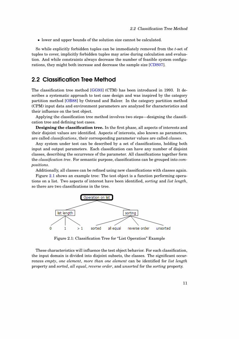
Additionally, all classes can be refined using new classifications with classes again.Figure 2.1 shows an example tree: The test object is a function performing opera-
tions on a list. Two aspects of interest have been identified, sorting and list length,so there are two classifications in the tree.
Figure 2.1: Classification Tree for “List Operation” Example
These characteristics will influence the test object behavior. For each classification,the input domain is divided into disjoint subsets, the classes. The significant occur-rences empty, one element, more than one element can be identified for list lengthproperty and sorted, all equal, reverse order, and unsorted for the sorting property.
11

2 Background
Thus, all parameters are classified and categorized.Definition of test cases. Having composed the classification tree, test cases are
defined by combining classes of different classifications. For each classification, a sig-nificant representative (class) is selected. Classifications and classes of classificationsare disjoint. Since classifications contain only disjoint values—obviously lists cannotbe sorted and unsorted at the same time—test cases cannot contain several values ofone classification. This small example would result in 12 different combinations totest.
2.3 Classification Tree Editor
Figure 2.2: CTE XL Layout
The Classification Tree Editor is a graphical editor to create and maintain clas-sification trees [WG93]. It supports the two steps of the classification tree methodwith distinct areas in its program window. First, the upper part of the program win-dow, the tree editor, is used to span classification trees. Then, the lower part of theprogram window, containing combination table and test case tree, is used to actuallyspecify test cases.
Lehmann and Wegener have extended the editor [LW00] to adopt results from thefield of combinatorial interaction testing [NL11], which allows the automatic gener-ation of test suites after the specification of the system under test has been given.
A screenshot of the extended classification tree editor (CTE XL) is provided inFigure 2.2.
The tree editor is located in the center of the application. The graphical represen-tation of classification tree elements is as follows:
12

2.4 Dependencies
• The root node has rounded corners.
• Classifications have a thin border.
• Classes do not have any border.
• Compositions have a thick border.
The lower part consists of a test case tree on the left and the combination table onthe right.
In the combination table, the tester can select and combine the classes for a testcase. Selected classes are represented by a solid cycle. When there is no selectedclass in a classification yet, all classes are marked with a question mark.
The test case tree is on the left side. It is used to create and edit test cases. Testcases are represented by a cycle and can be combined into test groups. Test groupsare represented by a small folder icon. Test groups can contain further test groups.
Test sequences can also be defined in CTE XL. In contrast to atomic test cases,test sequences consist of several test steps. A sequence is represented with a smalltriangle, containing test steps with a small arrow. When executing a test sequence,it passes, if all test steps successively pass in the order they are defined.
2.4 Dependencies
With the introduction of combinatorial aspects, Lehmann and Wegener also intro-duced dependency rules for the CTE XL [LW00]. Dependency rules are used to spec-ify constraints between different elements of the classification tree.
An example for this scenario is list processing (Figure 2.3).
Figure 2.3: Classification Tree for the “Element Counting" Example
The algorithm searches a given list for a given pivot element. The list can be empty(length = 0), consist of one element (length = 1), or contain more than one element(length > 1); resulting in three different list lengths. If the list contains one element
13
2 Background
only, it can be either the pivot element or not. With the list consisting of more thanone element, the parameter contains element can assume the values no, once, ormany. The last influence on the algorithm is list sorting. The parameter sorting oflists can be sorted, all equal, reverse order, or unsorted.
There are several dependencies here. Since length > 1 is the only scenario wheresorting applies it can be modeled as implicit dependency.
If list sorting is all equal, the list can contain the element several times or not atall, but not just once. This dependency cannot be modeled in the tree, but has to bespecified as an explicit dependency for this classification tree.
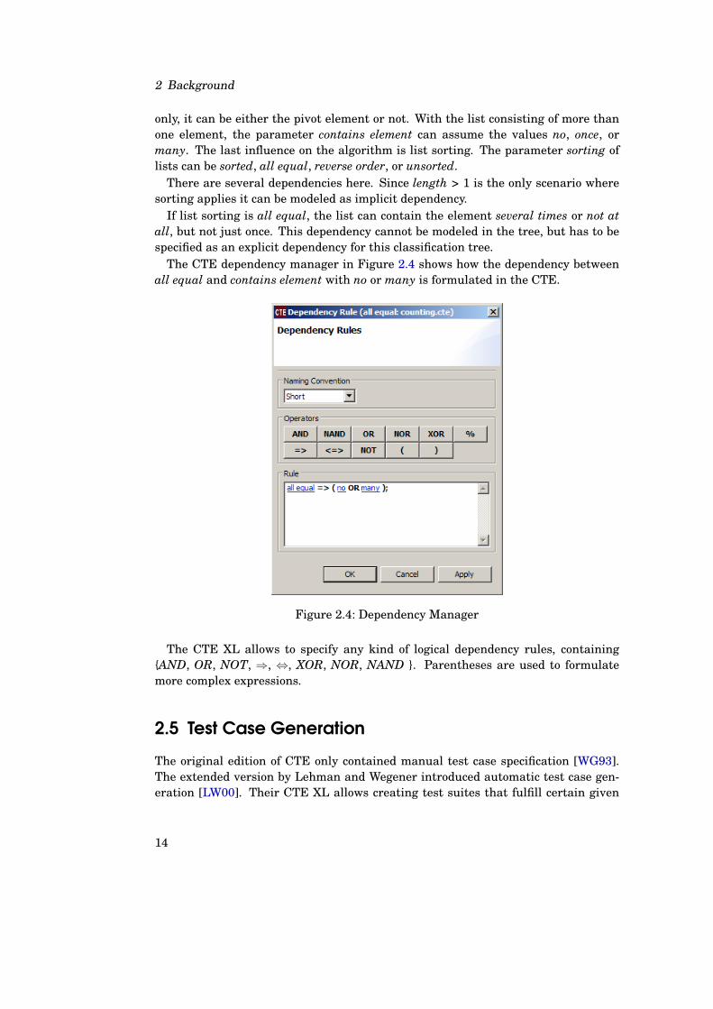
The CTE dependency manager in Figure 2.4 shows how the dependency betweenall equal and contains element with no or many is formulated in the CTE.
Figure 2.4: Dependency Manager
The CTE XL allows to specify any kind of logical dependency rules, containing{AND, OR, NOT, ⇒, ⇔, XOR, NOR, NAND }. Parentheses are used to formulatemore complex expressions.
2.5 Test Case Generation
The original edition of CTE only contained manual test case specification [WG93].The extended version by Lehman and Wegener introduced automatic test case gen-eration [LW00]. Their CTE XL allows creating test suites that fulfill certain given
14

2.5 Test Case Generation
coverage levels. Supported coverage levels are minimal combination, pairwise com-bination, threewise combination, and complete combination.
A screenshot of the CTE XL test case generator is provided in Figure 2.5. Theminimal combination is represented by the + sign, the complete combination by the* sign. The screenshot shows a generation rule for the list example from Figure 2.1demanding the complete combination of list length and sorting.
Figure 2.5: Test Case Generator
2.5.1 Test Case Generation with Dependencies
One motivation for this work is the handling of dependencies in CTE XL. Normally,CTE XL handles dependencies quite well and takes care of them during test case gen-eration. There is, however, a problem with concatenated dependency rules: Whenthere are dependency rules which depend on the fulfillment of other dependencyrules, CTE XL sometimes tends to not completely handle all dependency rules si-multaneously. This behavior results in test suites containing invalid test cases. Aninvalid test case is a test case violating at least one dependency rule.
A simple example is the classification tree given in Figure 2.6 consisting of fourclassifications with two classes each. It shall have three dependency rules d1 = a→!c,
15

2 Background
Figure 2.6: Dependency Example
d2 = g → c and d3 = e → c. In this simple situation, CTE XL is not capable of gener-ating an all-valid test suite covering all pairs between param1, param2, param3, andparam4, but always creates a test suite containing invalid test cases due to invalid(forbidden) combinations of classes.
Additionally, the handling of dependency rules resulting in an empty test suite,because all test cases are invalid and thus the number of valid test cases is zero, isnot working correctly in CTE XL. For these scenarios, CTE XL still creates test suites,although the tool recognizes, that all containing test cases are invalid afterwards.
2.6 Test Sequence Generation
In [CDFY99] Conrad et al. present the automatic import of Simulink Models intoclassification trees. They use imported models for systematic determination of testscenarios. Test scenarios can be either test sequences or test cases.
A test scenario is a series of stimuli in a certain order and with assigned dura-tions. They use the combination table of the classification tree editor to define signalcourses. With additional metadata, they annotate the type of the course. Supportedcourse types are step, ramp and spline, with step being the default. Their systemcan be used to model both discrete and continuous signals. The reuse of modelinginformation from the development for test activities reduces time and costs for testmodeling.
The approach is further described in [Con05]. The work focuses on the integrationof test scenarios for embedded systems into the development process. Model-basedspecification, design and implementation are in place, but testing still can be im-proved. Since testing all feasible combinations is nearly impossible, a good selectionof test scenarios determines extent and quality of the whole test. The automatic cre-ation is desirable, but only yet possible to a limited extent, which leads to largelymanual test design. The problems of ad-hoc test scenario selections are redundancyand possible gaps. They are typically in a very concrete notation with a low level ofabstraction, making reuse difficult.
The given example tree from Figure 2.7 results in the parallel state machine given
16

2.6 Test Sequence Generation
Figure 2.7: Example Tree for Conrad’s Approach
in Figure 2.8. The notation and syntax follows [Har87].
Figure 2.8: Resulting Parallel State Machine
The proposed solution is a model-based testing (MBT) approach [EFW01] based onan abstract model of the input data. The input partitioning of this approach impliesa parallel state machine model. Each classification forms one of the parallel parts(AND-states) of the state machine. The states denote the individual equivalenceclasses defined for the classification. Test sequences can be viewed as paths throughsuch a test model.
Making the underlaying test model explicit allows us to compare Conrad’s ap-proach with other MBT approaches. Furthermore, the test model can be used toformalize different coverage criteria. Conrad suggests the systematic scenario selec-tion based on the functional specification.
Current tools supporting the classification tree method do only allow manual defi-nition of test sequences. There are no generation rules for test sequence generation;desired coverage levels for a set of test sequences cannot be specified. Dependencyrules to describe constraints between single steps of test sequences do not exist andcan therefore not be checked.
17


3 Related Work
In this chapter, we give an overview of related work. First, we summarize combi-natorial and pairwise testing. Then, fundamental work on test sequence generationand validation is described. We then draw conclusions from the related work.
3.1 Combinatorial Testing
Combinatorial Interaction Testing (CIT [CSR06]) is an effective testing approach fordetecting failures caused by certain combinations of components or input values. Thetester identifies the relevant test aspects and defines corresponding classes. Theseclasses are called parameters, their elements are called values. We assume the pa-rameters to be disjoint sets. A test case is a set of n values, one for each parameter.In the classification tree method, the parameters are called classifications, the valuesare called classes.
CIT is used to determine a smallest possible subset of tests that covers all com-binations of values specified by a coverage criterion with at least one test case. Acoverage criterion is defined by its strength t that determines the degree of parame-ter interaction and assumes that all parameters are considered.
The most common coverage criterion is 2-wise (or pairwise) testing. It is fulfilled,if all possible pairs of values are covered by at least one test case in the result testset. A large number of CIT approaches have been presented in the past. An overviewand classification of approaches can be found in [GOA05] and [KLK08], while [NL11]provide a recent survey of CIT and its evolution. A survey that focuses on CIT withconstraints is given in [CDS07]. Nearly all publications investigate pairwise combi-nation methods, but most of them can be extended to arbitrary t-combinations.
The test generation techniques can be classified into algebraic, greedy and meta-heuristic search approaches [CDS07, NL11].
3.1.1 Greedy Approaches
AETG
The automatic efficient test generator (AETG) uses a random greedy algorithm. Ithas been developed at Bellcore and presented by Cohen et al. [CDFP97]. A determin-istic variant is also available. Candidates M are generated by selecting the value thatis contained in most not yet covered t-tuples. The candidate c is chosen which coversmost new t-tuples. A parameter order is created and used to select from each param-eter the parameter value with most of the not yet covered t-tuples. AETG supports
19

3 Related Work
pairwise, triple and n-wise. AETG does support seeding and dependencies [CDFP97],but resulting implementation and performance remain unclear. Mixed-strength gen-eration is realized using seeding.
ATGT
The ASM test generation tool (ATGT) uses a logic-based approach [CG10]. The test-ing problem is mapped onto a model-checking problem. Test predicates are used toformalize combinatorial testing as a logical problem. Then an external formal logictool is used to solve it. Constraints are expressed as logical predicates as well, whichis an advantage over plain tuple exclusion. Constraint processing is done as part ofthe solving process avoiding expensive pre- or post-processing steps. Test cases aregenerated as counter examples one at a time while a monitoring process keeps trackof covered tuples.
A collecting technique groups not covered tuples to assist in finding good test casesin each step. Final reduction is performed on the complete test suite to avoid redun-dant test cases. The algorithm is non-deterministic since the tool randomly selectsthe next predicates for test case generation.
DDA
The deterministic density algorithm (DDA) is an iterative algorithm that generatesa test set for pairwise class coverage [CC04].
Each test case is constructed stepwise using a greedy algorithm. Initially, the pa-rameter with the largest factor density is selected. The parameter’s value is selectedby its level density.
If there is more than one paramenter with the same level density available, lexi-cographical order is used as a tie-breaking rule. The concepts of densities have thefollowing meaning [BC07]:
• Factor density calculates the expected value of not yet covered pairs per param-eter.
• Level density calculates the expected value of not yet covered pairs per param-eter value.
DDA guarantees logarithmic growth of the test suite size in relation to the numberof parameters [CC04].
There is a prioritizing variant of DDA which respects the importance of pairs dur-ing test case generation [BC06]. The prioritization weights are given by the user.The goal is to cover pairs with high weights early in test case generation. This mod-ification of the DDA for prioritizing test case generation consists of modified densityfunctions. The weighted density function calculates the expected value of weights ofcovered pairs in relation to the number of not yet covered pairs [BC06].
Both variants skip dependencies for performance reasons.
20

3.1 Combinatorial Testing
IPO
In parameter order (IPO) was presented by Lei and Tai [LT98]. Their algorithm gen-erates test suites in a constructive way. First a test suite is created to cover onlythe first two parameters p1 and p2. Then all additional parameters are taken intoaccount one after another (p3 ... pn). Taking into account additional parameters in-cludes two steps: horizontal growth (the enhancement of existing test cases to haveparameter values for newly integrated parameters) and vertical growth (adding newtest cases for new combinations (tuples) due to the introduction of parameters). IPOonly supports pairwise combination. It does not support dependencies between pa-rameters. The PairTest tool implements IPO.
PICT
Pairwise independent combinatorial testing (PICT) has been developed by Czerwonka.The generation process consists of two phases: preparation and generation [Cze06].
In the preparation phase, all possible parameter interactions are calculated andlists of tuples are composed. Each tuple is marked either uncovered, covered, orexcluded.
In the generation phase, test cases are built using a deterministic, heuristic greedy-algorithm. First, seed combinations are added to the current test case candidate aslong as they do not violate constraints. From the list with most tuples still uncovered,the first uncovered tuple is chosen. Since tuples have components from different lists(e.g. at least two for t = 2), the algorithm iterates through the list(s) of the otherpart(s) of the tuple. From this second list, tuples are added that do not violate theexisting test case configuration. If no new tuple can be taken (because all tuples havealready been used in other test cases), an already covered tuple is randomly chosento be reused. From each list tuples are taken, so that in the end, there is a selectionfor each list and the test case is complete. Generation finishes when there are nomore uncovered tuples left.
PICT supports seeding, dependencies and t-wise generation for any t. Mixed-strength criteria and parameter hierarchies are also possible with PICT.
Spec Explorer
Spec Explorer is a CIT generator and a path covering tool [GQW+09]. The solutiondiffers from others as the algorithm generates interaction combination based solelyon constraint resolution and model enumeration as provided by the constraint en-gine. In contrast to other approaches which typically work bottom-up (single testcases are created until coverage is completed), the algorithm creates the result set ina top-down fashion as the solver enumerates combinations. The approach supportsconstraints and uses heuristics heavily to overcome scalability issues when inter-nally storing the complete set of all possible combinations. It goes one step furtherthan ATGT [CG10] by avoiding reduction steps.
21

3 Related Work
The benchmarks and comparisons by others [SRG11], however, show that perfor-mance in terms of result set size needs further improvements. Test generation takesmuch longer than with the other approaches presented in this section.
3.1.2 Meta-heuristic Search Approaches
CASA
A technique for compiling constraints into a Boolean satisfiability (SAT) problem andintegrating constraint checking into existing algorithms is presented in [CDS07].The technique is integrated into both greedy and simulated annealing algorithmsand experiences with its application are reported. The authors provide description forconstraint handling, their prototype is proposed to be extendable to other algorithmsand to incorporate constraints into algorithms for construction constrained coveringarrays.
In the simulated annealing algorithm (as an example for meta-heuristic searches),the outer search is a binary search because result set size is not known at the start.Therefore it needs multiple runs to find a good result set size. In each inner search,the actual annealing takes place. An array is filled with valid values and then grad-ually improved to become a covering array. Constraints can be given as Booleanformulae allowing SAT solvers to be used for checking. Forbidden tuples are markedas already covered to support the algorithm.
The initial approach had some scaling issues, so major improvements resulted inthe final Covering Arrays by Simulated Annealing (CASA) approach [GCD09]. It usesone side narrowing now instead of the binary search and checking of single items hasbeen enhanced to check for slightly larger groups.
3.1.3 Algebraic Approaches
MOLS
Test case generation for pairwise combination can be performed using Mutually Or-thogonal Latin Square (MOLS) [MN05]. A Latin square of order m is an m × mmatrix. Each field in the matrix is filled by one of the m different numbers. In eachcolumn and each row, each number occurs exactly once.
The first step is to find the MOLSs of a given order. The order of MOLSs is definedby the number of parameter values per parameter. The generation of test cases isthen done by reading the details from the MOLS. The algorithm and definitions aregiven in [MN05]. The problem with MOLS is that their computation is rarely trivial.For prime numbers and the power of prime numbers, there is an algebraic approach.For all other cases, there is no efficient way to create MOLS. If all parameters havethe same number of parameter values, the algorithm creates a reasonable set of testcases. If not, MOLSs are created with maximum order, which is the parameter withthe largest number of parameter values. This leads to many redundancies in theresulting test suite. However, there are methods to optimize these test suites [Wil02].
22

3.2 Test Sequence Generation and Validation
This approach does not support dependencies. Because of their fixed size and order,there is no way to incorporate additional information (e.g. semantics, weights ...) totest case generation.
3.2 Test Sequence Generation and Validation
Model checking aims to prove certain properties of program execution by completelyanalyzing its finite state model algorithmically [BE10, JM09]. Provided that themathematically defined properties apply to all possible states of the model, it isproven that the model satisfies the properties. However, when a property is violatedsomewhere, the model checker tries to provide a counter-example. Being the sequenceof states, the counter-example leads to the situation which violates the property. Abig problem with model checking is the state explosion problem: The number of statesmay grow very quickly when the program becomes more complex, increasing the totalnumber of possible interactions and values. Therefore, an important part of researchon model checking is state space reduction, to minimize the time required to traversethe entire state space.
The Partial-Order Reduction (POR) method is regarded as a successful method forreducing this state space [JM09]. Other methods in use are symbolic model check-ing, where construction of a very large state space is avoided by use of equivalentformulas in propositional logic, and bounded model checking, where construction ofthe state space is limited to a fixed number of steps.
Two temporal logics are compared and debated extensively [Var01], Linear tempo-ral logic (LTL) and Computation Tree Logic (CTL). Temporal logics describe modelproperties and can reduce the number of valid paths trough the model.
Heimdahl et al. briefly surveys a number of approaches in which test sequencesare generated using model checking techniques [HRV+03]. The common idea is touse the counter-example generation feature of model checkers to produce relevanttest sequences.
Krupp and Müller introduce an interesting application of CCTL logic for the ver-ification of manually created test sequences in classification trees [KM05]. Usinga real-time model checker, the test sequences and their transitions are verified bycombining I/O interval descriptions and CCTL expressions.
Several researchers propose other approaches for test sequence generation. Wim-mel et al. [WLPS00] propose a method of generating test sequences using proposi-tional logic.
Ural [Ura92] describes four formal methods for generating test sequences basedon a finite-state machine (FSM) description. The question to be answered by thesetest sequences is whether or not a given system implementation conforms to theFSM model of this system. Test sequences consisting of inputs and their expectedoutputs are derived from the FSM model of the system, after which the inputs can befed to the real system implementation. Finally, the outputs of the model and of theimplementation are compared.
23

3 Related Work
Bernard et al. [BLLP04] have done an extensive case study on test case generationusing a formal specification language called B. Using this machine-modeling lan-guage, a partial model of the GSM 11-11 specification has been built. After a systemof equivalent constraints was derived from this specification, a constraint solver isused to calculate boundary states and test cases.
Binder [Bin99] lists a number of different oracle patterns that can be used for soft-ware testing, including the simulation oracle pattern. The simulation oracle patternis used to simulate a system using only a simplified version of the system implemen-tation. Results of the simulation are then compared to the results of the real system.We can regard the formal model of the system as the simulation of the system fromwhich expected results are derived.
Geist et al. partition a test problem into aspects of interest to guide the searchfor test cases to interesting parts of the system [GFL+96], using temporal logic andBDDs instead of traditional graph-algorithmic models. The target is transistion cov-erage. Steps are a) building an FSM model of the test problem, b) definition of cov-erage model, and c) test generation. All FSM transitions are stored in a BDD forperformance reasons. Test cases are generated per transition. New test cases areevaluated for all included transitions and removed from the list of transitions to becovered. The result set size does not necessarily have a minimum number of testcases. The limitation of current coverage tools drives verification by simulation torely on massive simulations without an inherent way to drive the test generationprocess by coverage considerations. Geist et al. deem sysbolic exploration not to bea bottleneck. Their technique avoids state-space explosion. Their generation cre-ates many test sequences of medium length, so they propose future work on creationof longer test sequences. They see, however, a tradeoff between reduced simulationtime caused by setup conditions with longer test sequences and easier debugging andtracing with shorter test sequences. Therefore they suggest to make the maximumnumber of transitions per test sequence a user-configurable parameter.
Automatic test sequence generation and coverage criteria for testing of ASMs arediscussed by Gargantini and Riccobene [GR01].
Burton et al. present an approach to use formal specification from statecharts anda testing heuristic to automatically generate test cases [BCM01]. For all transitionsin the statechart a Z-representation is extracted. The internal Z-representation isthen used to create an internal representation. A test sequence is then created foreach state of the internal representation. There is no minimization of test sequences.
To generate tests from Z specifications, the disjunctive normal form (DNF) methodcan be used, although it is prone to state explosion [HHS03]. The authors propose toconstruct a classification tree from the Z specification and use the resulting tree fortest generation. There are several suggestions for constraint learning and efficienttree construction, although the main manual work of test case selection is left to thetester.
Windish has applied search-based testing to Stateflow Statecharts [Win08, Win10].A messy genetic algorithm (GA) is used to generate transition tours through Simulink
24

3.3 Conclusion
Stateflow models [OHY11]. Oh et al. identify two main challenges: Trigger blockscontaining timing constraints or counters and cyclic paths which might require sev-eral traversals before triggering a transition. A further problem is the a priori un-known length of the resulting tour. Stateflow models supports hierarchies and con-currences which they directly used to avoid sequentialization and therefore do notsuffer from state explosion.
A technique for test sequence generation is introduced by Kuhn et al.: They gen-erate event sequences for a given set of system events. They allow specifying t-way sequences, which includes all t-events being tested in every possible t-way or-der [KKL10].
Recent application of test sequence generation can be the state-based testing ofAJAX web applications [MTR08]. The authors apply model extraction and modellearning to AJAX web applications. The resulting FSM is then tested using concretedata from traces obtained during model learning.
3.3 Conclusion
There are only limited possibilities to support explicit prioritization of parametersand parameter values. The only known algorithm supporting prioritized test casegeneration is the deterministic density algorithm (DDA) published in [BC06], whichis an extension of [CC04]. The extended algorithm generates a test suite by succes-sively constructing single test cases. During test case construction it accounts for (1)uncovered pairs in the test suite generated so far and (2) user assigned weights. Pairswith higher weights are covered earlier than pairs with lower weights. For efficiencyreasons, this algorithm does not consider explicit dependencies. To our knowledge, itdoes not support any t-wise combination other than pairwise.
Therefore, we will design new test case generation algorithms for classificationtrees with incorporated prioritization weights. In [HRSR09] a first approach for com-bining classification trees with priorities has been presented.
Currently, there is no test sequence generation available for combinatorial testing.The only known approach is the t-way sequence generation [KKL10] which is limitedto combinations of parameter values of one parameter at a time and does not handleparameter interactions of several parameters.
For that reason, we will also design test sequence generation algorithms for classi-fication trees.
25

4 Enhancements
In this chapter, we design our enhancements for test case and test sequence gener-ation with the classification tree method. We select three prioritization models andgive a prioritization example to then qualify the classification tree (Section 4.1). Fordependency handling, we transform both the classification tree and its dependencyrules into an integrated data structure, a Binary Decision Diagram (Section 4.2). Af-terwards we use this data structure for dependency handling in prioritized test casegeneration (Section 4.3). Additionally, we exploit the data structure for a new deter-ministic test case generation (Section 4.4). For our new test sequence generation wedesign new dependency and generation rules (Section 4.5). Actual generation is thendone by converting the classification tree into a hierarchical concurrent finite statemachine and traversing it using a multi-agent system (Section 4.6).
4.1 Prioritization and Qualification
Prioritization is used to allow the assignment of values of importance to several clas-sification tree elements. The values of importance are called weights. To cover allkinds of test aspects, these weights can differ. Higher and lower weights should re-flect higher and lower importance, respectively. Consequently, we are able to comparethe elements of the classification tree to determine their importance under a giventest aspect and to prioritize test aspects during test case generation.
We analyzed several existing prioritization techniques. Elbaum et al. give goodoverviews of existing approaches [EMR02, ERKM04].
Many existing prioritization techniques are not applicable in the classification treefor methodical reasons. Among these can be that the level of abstraction does not fitor the required details are not included in the classification tree. For example, testcases cannot be optimized on state coverage since the classification tree method is ablack-box test design approach.
The following three models have been selected to provide a basis for prioritizationas they are applicable for the classification tree method:
• Prioritization based on a usage model [WPT95]: This prioritization tries toreflect usage distribution of all classes in terms of usage scenarios. Classes withhigh occurrence are assigned higher weights than classes with low occurrence.
• Prioritization based on an error model [EMR02]: This prioritization aims toreflect distribution of error probabilities of all classes. Classes with high prob-
27

4 Enhancements
ability of revealing an error are assigned higher weights than classes with lowprobability.
• Prioritization based on a risk model [Aml00]: This prioritization is similarto prioritization based on error model, but additionally takes error costs intoaccount. Risk is defined as the product of error probability and error costs.Classes with a high risk are assigned higher weights than classes with lowrisk.
The selected prioritization models will now be used for qualifying the classificationtree.
4.1.1 Example
We will use the following example throughout all prioritized generation algorithms.The example in figure 4.1 shows a classification tree for the system under test Adap-tive Cruise Control (ACC). Its task is to adapt the speed of a vehicle to keep a certaindistance to preceding vehicles. Three aspects of interest (Speed, Daylight and kindof Preceding Vehicle) have been identified for the system under test. These classifi-cations are direct children of the root node. The classifications are partitioned intoclasses which represent the partitioning of the concrete input values. In our examplethe refinement aspect Shape is identified for the class Car and it is divided furtherinto the two classes Limousine and Cabriolet.
Figure 4.1: Test Object ACC
For the qualification with different priority models, there are several things toconsider: Consistency is needed both locally (considering a class and all siblings) aswell as globally (interaction of classes from different classifications). Additionally,for combined constructs, such as class pairs and other tuples, a uniform calculationis needed. For refined elements, we also need to define a handling. The presence ofconstraints can have an impact on the priority model as well, so we need to clarifythis issue.
28

4.1 Prioritization and Qualification
4.1.2 Qualification with Usage Model
Occurrence Probability is always given for classes with respect to the parent classi-fication. For class c an occurrence value pc denotes the relative frequency for c incomparison to all sibling classes d, e, f .... The sum of all occurrence values pn for sib-lings from classification C must always be 1. We require that a value is given for allclasses of all classifications in the classification tree, before these values can be usedfor prioritized test generation. Occurrence values for siblings are directly compara-ble without normalization. Given that classifications are independent of each other,occurrence values from different classifications are also directly comparable. Underthis assumption, composed constructs, such as pairs, can be formed by multiplyingindividual values of all involved classes.
We define refined classes to be interpreted as conditioned probabilities. The actualvalue can then be calculated using the Bayes-Theorem.
Since handling of constraints is done without knowledge of priorities, the qualifi-cation of the classification tree has to be done with constraints in mind.
Figure 4.2: ACC Test Object with Occurrence Values
Occurrence values for the ACC example are given in Figure 4.2.
Table 4.1: Occurrence Probabilities for Class Pairslow medium high Day Night0.3 0.5 0.2 0.52 0.48
Motorcycle 0.05 0.015 0.025 0.01 0.026 0.024Limousine 0.63 0.189 0.315 0.126 0.3276 0.3024Cabriolet 0.07 0.021 0.035 0.014 0.0364 0.0336
Truck 0.25 0.075 0.125 0.05 0.13 0.12Day 0.52 0.156 0.26 0.104 - -
Night 0.48 0.144 0.24 0.096 - -
All expected occurrence probabilities for combined class pairs are given in Ta-ble 4.1.
29

4 Enhancements
4.1.3 Qualification with Error Model
Error Probability is always given as absolute values for classes without any relationto the parent classification. For class c an error value ec denotes the absolute valuefor c in comparison to all other classes d, e, f ... of the classification tree. We requirethat a value is given for all leaf classes in the classification tree, before these valuescan be used for prioritized test generation. Error values for siblings are directly com-parable without normalization, as well as error values from different classifications.Composed constructs, such as pairs, can be formed by multiplying individual valuesof all involved classes.
Since error values are independent of each other, we do not introduce a handlingfor refined classes as conditioned probabilities. Instead, we only allow error valueson leaf classes.
Again, handling of constraints is done without knowledge of priorities, so the qual-ification of the classification tree has to be done with constraints in mind.
Figure 4.3: ACC Test Object with Error Values
Error values for the ACC example are given in Figure 4.3.
Table 4.2: Error Probabilities for Class Pairslow medium high Day Night0.01 0.03 0.03 0.03 0.07
Motorcycle 0.13 0.0013 0.0039 0.0039 0.0039 0.0091Limousine 0.07 0.0007 0.0021 0.0021 0.0021 0.0049Cabriolet 0.1 0.001 0.003 0.003 0.003 0.007
Truck 0.05 0.0005 0.0015 0.0015 0.0015 0.0035Day 0.03 0.0003 0.0009 0.0009 - -
Night 0.07 0.0007 0.0021 0.0021 - -
All expected error probabilities for combined class pairs are given in Table 4.2.
30

4.1 Prioritization and Qualification
4.1.4 Qualification with Risk Model
Risk values are always given absolute for classes without any relation to the parentclassification. For class c a risk value rc denotes the absolute value for c in compari-son to all other classes d, e, f ... of the classification tree. Risk is given in two values,error probability and cost of an error. The actual risk, then, is the product of the two.We require that values are given for all leaf classes in the classification tree, beforethese values can be used for prioritized test generation. Risk values for siblings aredirectly comparable without normalization, as well as risk values from different clas-sifications. Composed constructs, such as tuples, can be formed by multiplying thecombining individual error probabilities with the summed individual costs.
Since risk values are independent of each other, we do not introduce a handlingfor refined classes as conditioned probabilities. Instead, we only allow risk values onleaf classes.
The qualification of the classification tree has to be done with constraints in mind,since handling of constraints is done without knowledge of priorities.
Figure 4.4: ACC Test Object with Cost Values
Cost values for the ACC example are given in Figure 4.4. The resulting risk valuesare given in Figure 4.5.
Table 4.3: Costs for Class Pairslow medium high Day Night
e10,000 e20,000 e30,000 e25,000 e25,000Motorcycle e10,000 e20,000 e30,000 e40,000 e35,000 e35,000Limousine e20,000 e30,000 e40,000 e50,000 e45,000 e45,000Cabriolet e30,000 e40,000 e50,000 e60,000 e55,000 e55,000
Truck e40,000 e50,000 e60,000 e70,000 e65,000 e65,000Day e25,000 e35,000 e45,000 e55,000 - -
Night e25,000 e35,000 e45,000 e55,000 - -
All expected costs for combined class pairs are given in Table 4.3.All expected risks for combined class pairs are given in Table 4.4.
31
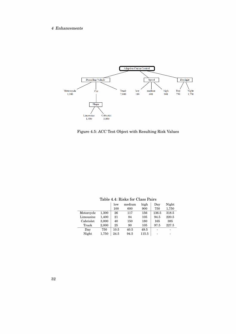
4 Enhancements
Figure 4.5: ACC Test Object with Resulting Risk Values
Table 4.4: Risks for Class Pairslow medium high Day Night100 600 900 750 1,750
Motorcycle 1,300 26 117 156 136.5 318.5Limousine 1,400 21 84 105 94.5 220.5Cabriolet 3,000 40 150 180 165 385
Truck 2,000 25 90 105 97.5 227.5Day 750 10.5 40.5 49.5 - -
Night 1,750 24.5 94.5 115.5 - -
32

4.2 Constraints Handling
4.1.5 Conclusion on Qualification
In Table 4.5 we provide additional values for occurrence probability, failure probabil-ity, failure costs, and the calculated risk for all leaf classes from our example.
Table 4.5: ACC Test Object InformationPreceding Vehicle
Motorcycle Limousine Cabriolet TruckUsage 0.05 0.63 0.07 0.25Failure 0.13 0.07 0.1 0.05Cost e10,000 e20,000 e30,000 e40,000Risk 1,300 1,400 3,000 2,000
Speed Daylightlow medium high Day Night
Usage 0.3 0.5 0.2 0.52 0.48Failure 0.01 0.03 0.03 0.03 0.07Cost e10,000 e20,000 e30,000 e25,000 e25,000Risk 100 600 900 750 1750
Note the difference between the occurrence probability values in the table and thefigure for the subclasses of the class Car. We explained in previous sections thatthe occurrence probabilities for classes are conditional probabilities, having a refinedclass as an ancestor node in the classification tree. In our example the probability ofthe class Cabriolet is 0.1 only when the class Car is chosen. Therefore, the absoluteoccurrence probability for this class is 0.07.
As shown in Table 4.5 it is, for example, much more probable that the precedingvehicle is a Limousine. If we focus on finding errors connected to the most commonusage scenario, we will expect test cases covering the class Limousine to be moreimportant than those covering the class Cabriolet. But if we focus on finding errorsthat have a high risk, we prefer test cases covering the class Cabriolet since it isassociated with the highest risk.
4.2 Constraints Handling
Classification trees can have implicit dependency rules in terms of refinements. Classescan have ancestor classifications with only local validity [GG93].
In the example from Section 4.1.1, the class Car has a refinement in terms of theclassification Shape (Figure 4.1). The test aspect Shape therefore only applies if andonly if the Preceding Vehicle is a Car. If it is a Truck or a Motorcycle, the classificationShape does not apply because Car has not been selected.
In contrast to implicit dependency rules in the classification tree method, the clas-sification tree editor CTE XL also allows the specification of explicit dependencyrules [LW00].
Explicit dependency rules allow specifying details of the test system, which seemto be orthogonal to the classification tree. It is possible to exclude combinations of
33

4 Enhancements
classes from different classifications, for example.For our example, we will now introduce two dependency rules. First we require,
that Motorcycles can only occur during the day, or more formal:
D1 = Motorcycle→ Day
Additionally we assume, that Trucks cannot drive with a high Speed:
D2 = Truck→ ¬high
These explicit dependency rules are heavily used by test engineers, but they areproblematic during test case generation. In test case generation, there needs to be acheck for validity making the whole test generation process a complicated task.
For test case generations, there are three different ways of handling explicit de-pendency rules: afterwards, during, and beforehand.
Handling after Test Case Generation
The simplest realization is the handling of dependencies just after the actual testcase generation. A normal, regular test case generation is performed, while com-pletely ignoring any dependency rules. When the generation is finished, each testcase is checked for validity. Invalid test cases are eliminated and new test cases aregenerated for the now missing tuples, if needed.
One disadvantage of this method is that there might not be any valid test at allcontaining the missing tuple, so invalid test cases will be generated again and again.The test case selection has no connection to the validity of test cases, checking andfiltering is performed afterwards. This approach is only applicable for small testproblems, where all possible combinations can be tried.
Immediate Handling during Test Case Generation
The advantage of this approach is the handling of dependency rules during test casegeneration. This approach will generate only valid test cases, so there is no needfor checking and filtering afterwards. This approach, however, requires numerousoperations. When composing a single test case, there needs to be a check for validityafter each single addition of test elements.
For example, an existing valid test case fragment containing class ai from classifi-cation A needs to be re-evaluated again when class bj from classification B is aboutto be added, to check, if ai and bj can co-exist.
This approach ensures that only valid test cases are generated. The validity checks,however, are rather expensive; they need time. Combinations of classes are evalu-ated as long as a valid combination is found, which in the worst case might be thelast available combination.
34

4.2 Constraints Handling
Handling before Actual Test Case Generation
This approach allows the test case generation without taking care of dependencyrules, since there are only valid combinations in the classification tree. Invalid com-binations do not exist in the tree. There is only one checking and filtering operationbefore the actual test case generation. There is no need for filtering after the testcase generation and there are no expensive comparison operations during test casegeneration. The actual test case generation therefore is rather cheap, the initialpreparation of the tree, however, might need additional effort.
4.2.1 Tree Transformation
We are going to present approaches for tree preparation. We require the followingconditions to be met:
• The test case generation is performed on a tree without explicit dependencies.
• A prepared tree must have the same semantics as the original tree.
• Transformations must be deterministic. The transformation of equal trees re-sults in the same result.
We use the mechanism of refinements to transform tree and explicit dependencyrules into a classification tree with only implicit dependencies. Refinements are usedto model aspects, which only apply for certain classes.
We see two tracks here:
• Transformation of only those tree elements, which are affected by dependencyrules.
• Full transformation.
Limited Transformation
The approach is rather simple. For all classifications that are part of dependencyrules, we perform the following:
• The first classification in the tree remains.
• To all its classes, copies of the second classification are attached.
• For the classes of these clones, copies of the third classification are created andattached, and so on.
In the end, the tree has the same levels of refinements as it had parallel classifica-tions at the beginning. For all leaf classes, there is only one check for validity.
This tree fulfills all three requirements: There are no additional explicit require-ments in the tree. The resulting tree has the same semantics as the original tree. We,
35

4 Enhancements
however, need to introduce an interpretation for classification-clones. Their interpre-tation is trivial, we treat copies the same way as originals. Determinism is gained byproviding a fixed transformation order. The effort of transformation is determined bythe number of dependency rules. For few rules, the resulting number of leaf classes(and therefore validity checks) is low. For many rules, effort will rise to the full trans-formation approach, especially if all classifications are part of dependency rules.
Full Transformation
The transformation process is rather trivial. Instead of handling only classificationsthat are part of dependency rules, we simply take all classifications of the classifica-tion tree here.
This also meets our three requirements: There are no additional explicit require-ments in the tree. The resulting tree has the same semantics as the original tree.We, again, need to introduce an interpretation for classification-clones, which, again,is trivial, since we treat copies the same way as originals. Determinism is gained byproviding a fixed transformation order. The transformation is very laborious, espe-cially for trees with only few dependency rules, as there are many leaf classes to bechecked afterwards.
4.2.2 Approach
Arriving here, we decided to convert classification trees into logical expressions forBinary Decision Diagrams (BDD). Binary Decision Diagrams [Lee59] can be usedto represent Boolean functions as compact data structures. We use the most com-mon variant of BDDs, reduced ordered binary decision diagrams (ROBDD), and usethe term BDD for simplicity. ROBDDs feature variable ordering and graph reduc-tion [Bry86].
We perform a transformation of the classification tree to Binary Decision Diagramsfrom the root of the tree down to all leafs of the classification tree. For each elementin the classification tree, there is a logical equivalent.
Classifications
In any classification C, exactly one class c is selected.
Figure 4.6: Classification C with Classes (c1, c2, . . . , cn)
The classification C with classes (c1, c2, . . . , cn) (Figure 4.6) results in:
36
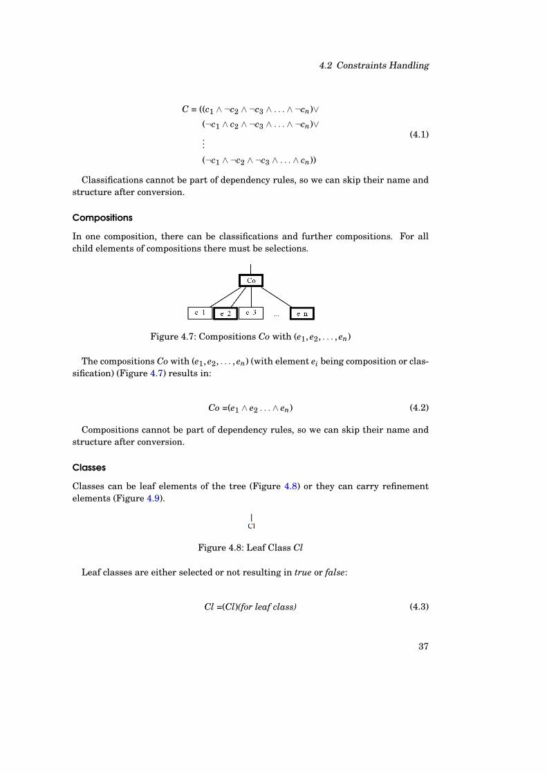
4.2 Constraints Handling
C = ((c1 ∧ ¬c2 ∧ ¬c3 ∧ . . . ∧ ¬cn)∨(¬c1 ∧ c2 ∧ ¬c3 ∧ . . . ∧ ¬cn)∨...
(¬c1 ∧ ¬c2 ∧ ¬c3 ∧ . . . ∧ cn))
(4.1)
Classifications cannot be part of dependency rules, so we can skip their name andstructure after conversion.
Compositions
In one composition, there can be classifications and further compositions. For allchild elements of compositions there must be selections.
Figure 4.7: Compositions Co with (e1, e2, . . . , en)
The compositions Co with (e1, e2, . . . , en) (with element ei being composition or clas-sification) (Figure 4.7) results in:
Co =(e1 ∧ e2 . . . ∧ en) (4.2)
Compositions cannot be part of dependency rules, so we can skip their name andstructure after conversion.
Classes
Classes can be leaf elements of the tree (Figure 4.8) or they can carry refinementelements (Figure 4.9).
Figure 4.8: Leaf Class Cl
Leaf classes are either selected or not resulting in true or false:
Cl =(Cl)(for leaf class) (4.3)
37

4 Enhancements
Figure 4.9: Class Cl with Refinements (E1, E2, . . . , En)
Refined classes can also be true or false.If they are true, they are treated like compositions. If they are false, all sub classes
are also false.The class Cl with (E1, E2, . . . , En) (with element Ei being composition or classifica-
tion), results in:
with Cl = true
Cl = (E1 ∧ E2 ∧ . . . ∧ En)
else
Cl = (¬e11 ∧ ¬e12 ∧ . . . ∧ ¬e1m∧¬e21 ∧ ¬e22 ∧ . . . ∧ ¬e2o∧...
¬en1 ∧ ¬en2 ∧ . . . ∧ ¬enq )
(4.4)
After transformation of the tree, dependency rules (D1 . . .Dn) can be attached tothe expression E with the ∧-operator:
ED = (E ∧D1 ∧ . . . ∧Dn) (4.5)
This expression now contains all valid test cases. Its construction, however, doesnot require to calculate or enumerate all assignments.
4.2.3 Example
We will now apply the rules from the previous section and transform the classifica-tion tree from Section 4.1.1 (Figure 4.1). The root node is a composition, so usingFormula 4.2 the starting Boolean expression is:
ACC = PrecedingVehicle ∧ Speed ∧Daylight (4.6)
Using Formula 4.1, we then transform the classifications Preceding Vehicle, Speedand Daylight:
38

4.2 Constraints Handling
PrecedingVehicle =(Mot ∧ ¬Car ∧ ¬Tru)∨(¬Mot ∧ Car ∧ ¬Tru)∨(¬Mot ∧ ¬Car ∧ Tru)
Speed =(low ∧ ¬med ∧ ¬hi)∨(¬low ∧med ∧ ¬hi)∨(¬low ∧ ¬med ∧ hi)
Daylight =(Day ∧ ¬Nit) ∨ (¬Day ∧Nit)
(4.7)
All classes are leaf classes except class Car. For Car, we need two variants, aregular and a negated one. Using the first part of Formula 4.4 and Formula 4.1, theregular variant is created:
Car = Shape
= (Lim ∧ ¬Cab) ∨ (¬Lim ∧ Cab)(4.8)
Using the second part of Formula 4.4 results in the negated variant:
¬Car = (¬Lim ∧ ¬Cab) (4.9)
Putting it all together:
ACC =PrecedingVehicle ∧ Speed ∧Daylight
=((Mot ∧ ¬Car ∧ ¬Tru) ∨ (¬Mot ∧ Car ∧ ¬Tru) ∨ (¬Mot ∧ ¬Car ∧ Tru))∧
((low ∧ ¬med ∧ ¬hi) ∨ (¬low ∧med ∧ ¬hi) ∨ (¬low ∧ ¬med ∧ hi))∧
((Day ∧ ¬Nit) ∨ (¬Day ∧Nit))
=((Mot ∧ (¬Lim ∧ ¬Cab) ∧ ¬Tru) ∨ (¬Mot ∧ (¬Lim ∧ ¬Cab) ∧ Tru)∨
(¬Mot ∧ ((Lim ∧ ¬Cab) ∨ (¬Lim ∧ Cab)) ∧ ¬Tru))∧
((low ∧ ¬med ∧ ¬hi) ∨ (¬low ∧med ∧ ¬hi) ∨ (¬low ∧ ¬med ∧ hi))∧
((Day ∧ ¬Nit) ∨ (¬Day ∧Nit))(4.10)
As defined in Formula 4.5, the two dependency rules D1 and D2 can simply be
39

4 Enhancements
attached:
ACCD =ACC ∧D1 ∧D2
=ACC∧
(Mot→ Day)∧
(Tru→ ¬hi)
=((Mot ∧ (¬Lim ∧ ¬Cab) ∧ ¬Tru) ∨ (¬Mot ∧ (¬Lim ∧ ¬Cab) ∧ Tru)∨(¬Mot ∧ ((Lim ∧ ¬Cab) ∨ (¬Lim ∧ Cab)) ∧ ¬Tru))∧((low ∧ ¬med ∧ ¬hi) ∨ (¬low ∧med ∧ ¬hi) ∨ (¬low ∧ ¬med ∧ hi))∧
((Day ∧ ¬Nit) ∨ (¬Day ∧Nit))∧
(Mot→ Day)∧
(Tru→ ¬hi)
(4.11)
In the resulting Formula 4.11, each valid assignment of ACCD now holds a validtest case.
4.3 Prioritized Generation
For the now quantified classification trees, new combination rules need to be de-signed. These new combination rules respect the weights assigned to the classesin the classification tree. We will introduce the following new prioritizing combina-tion rules: Prioritized minimal combination, prioritized pairwise combination, andclass-based statistical combination. For each combination rule, we will define re-quirements for the resulting test suite. We will then design algorithms for test casegeneration. Test case coverage criteria will be given where they apply.
4.3.1 Prioritized Minimal Combination
The basic algorithm used to generate minimal combinations creates a test set cov-ering each class at least once. At each step, it generates one test case by selectingsingle classes from all classifications. It stops generating test cases as soon as allclasses are covered, but does not take the order of covering them into account. Weextend the algorithm so that it selects classes based on their weights. Classes witha high weight are of great importance for our test objective and will be chosen first.The distribution defined by class weights is used to reselect classes of classificationwith all its classes already covered by the test suite generated. We compare the em-pirical class distribution of such a classification with the class distribution given inthe generated test suite and choose the class that is most underrepresented in thetest suite generated so far.
Coverage Criteria
We define coverage criteria to
• measure to which degree the system under test can be tested with an optimizedtest suite, and
40

4.3 Prioritized Generation
• to compare optimized test suites of different sizes to determine the benefit ofadditional test resources.
We define two different criteria that measure the degree to which the classes (eachused coverage, EUC) and the weights are covered (weight coverage, WC):
EUC =number of covered classes
number of coverable classes
WC =sum of weights of covered classes
sum of weights of all coverable classes
Both metrics are relative, i.e. consider the fact that classes may not be coverablebecause of dependencies. To understand the need of both criteria we consider a clas-sification with 10 classes where eight have a very small weight. If the test suiteconsists of only two test cases covering the two classes with the highest weights, weget a small EUC value. But the WC value for all other test suites of size two selectingother classes from this classification will be lower. Using our coverage criteria, thetester can define test end criteria and measure the progress in the test process.
Algorithm
We split the calculation into two algorithms. The top level algorithm calculates thecomplete test suite. It gets the set M of all valid test cases as input parameter andinitializes the set B of all coverable classes extracting them from the set M. Then ititeratively
• passes both sets B and M to the algorithm that calculates the next test case t,
• deletes t from set M and adds it to the result list, and
• deletes all classes covered by t from set B.
The algorithm stops as soon as all classes are covered, i.e. when set B is empty. Aclass c is only deleted from B, if a test case containing c has been added to the resultlist. The test cases are selected from the set of valid test cases, i.e. we add only validtest cases to the result list. The algorithm does not consider uncoverable classes sinceuncoverable classes do not appear in the set B.
The algorithm for defining a single test case t (Figure 4.10) gets at each call a copyof the updated set B of all classes not yet covered and a copy of the updated set M ofall valid test cases still available. It reduces M so that it finally contains only one testcase. In each iteration, the class k with the highest weight of all still available classesis selected from B (Line 5), taking only already selected classifications into account.This k is used to further restrict M (Line 7). If the restriction with k fails, i.e. thereis no test case left in M for the so far selected classes including k, the algorithmsbacktracks (Line 10) and restarts selecting a new class. If a classification is alreadycovered, there will be no k. In this case, all test cases left in M are compared and thetest case that contains the most underrepresented classes is chosen (Line 14).
41

4 Enhancements
1: M //set of available test cases2: B //set of classes not yet covered3: while (|M| > 1) do4: N = copy M for backtracking5: k = select class from B6: if (k was found) then7: M = filter M with k8: B = delete k from B9: if (M is empty) then
10: M = N //backtracking11: end if12: else13: //check underrepresentation14: t = choose test case from M15: M = {t}16: end if17: end while18: t = getSingleElement(M)19: return t
Figure 4.10: Test Case Generation Algorithm for Prioritizing Minimal Combination
Every test case returned by generateNextTestCase contains the class with the high-est weight compared to all classes not yet covered. After n test case generation stepsthe presented top level algorithm returns a test suite that covers at least the n mostimportant classes. At each generation step as many new classes as possible are se-lected, i.e. coverage and weight of classes are maximized.
Example
In Table 4.6 the test suite generated by the presented algorithm is shown for our ex-ample using the risk value annotations from Table 4.5 and without any user-defineddependencies. The test suite covers all classes at least once. The classes Cabriolet,high and Night are covered by the first test case since these classes are associatedwith the highest risk values. In the last two test cases the class Night is reselectedfor the classification Daylight. The algorithm did not choose class Day since its riskvalue is much lower than the value for class Night. Since we want to detect failureswith a high risk we prefer test cases that cover classes with high risk values.
Table 4.6: Resulting PMC Test Suite for the Risk ModelPrec. Vehicle Speed Daylight EUC WC
#1 Cabriolet high Night 0.3 0.48#2 Truck medium Day 0.6 0.76#3 Limousine low Night 0.89 0.8#4 Motorcycle high Night 1 1
The last two columns in Table 4.6 contain the coverage values for the test suitecontaining only the test cases up to that row. We can see that we cover almost half
42
4.3 Prioritized Generation
of the risk values sum with only one test case. Comparing both values EUC and WChelps finding the best test suite size with respect to test resources.
Discussion
The prioritized minimal combination allows adapting the test suite to available re-sources. In an optimized test suite, classes with high weight are covered and theglobal coverage of new classes and weights is maximized. If there are no new classesto cover under one classification, a test suite is composed based on the distribution ofweights. Whenever there are less classes under one classification than the numberof total existing test cases exist, classes with higher weights reoccur in the test suite.Without optimization, a test suite created with the prioritizing minimal combinationcontains all classes of the classification tree, if there are no dependency rules.
Dividing the number of covered classes by the number of coverable classes givesa good criterion for absolute coverage. Dividing the sum of all weights of coveredclasses by the sum of all weights of coverable classes gives a good criterion for relativecoverage. Due to coverage criteria all results are measurable.
4.3.2 Prioritized Pairwise Combination
The basic pairwise algorithm iteratively generates test cases until all possible classpairs are covered by at least one test case. At each generation step, it tries to select asmany new pairs as possible for the test case, but does not take any order of coveringthem into account. We extend the algorithm so that test cases covering pairs ofclasses with high weights are generated before those containing pairs of classes withsmaller weights.
Coverage Criteria
We define two different criteria, in analogy to the PMC coverage criteria, that mea-sure to which degree the class pairs (each used coverage, EUC) and to which degreethe weights are covered (weight coverage, WC):
EUC =number of covered class pairs
number of coverable class pairs
WC =sum of weights of covered class pairs
sum of weights of all coverable class pairs
Both metrics are again relative.
Algorithm
Our prioritization pairwise combination algorithm is based on pair weights that wedefine for the different prioritization models. For the usage and the failure model wedefine the weight of a pair (ci, cj) as the product of the weights assigned to ci and cj.
43
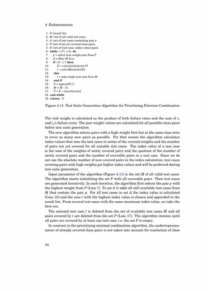
4 Enhancements
1: S //result list2: M //set of all valid test cases3: A //set of test cases containing pair p4: P //set of not yet covered class pairs5: D //set of (test case, index value) pairs6: while (|P| > 0) do7: p = select max weight pair from P8: A = filter M by p9: if |A| > 1 then
10: D = calculateIndex(A, P)11: t = selectMaxIndex(D)12: else13: t = take single test case from M14: end if15: S = append(S, t)16: M = M – {t}17: P = P – {classPairs(t)}18: end while19: return S
Figure 4.11: Test Suite Generation Algorithm for Prioritizing Pairwise Combination
The risk weight is calculated as the product of both failure rates and the sum of ciand cj’s failure costs. The pair weight values are calculated for all possible class pairsbefore test suite generation.
The new algorithm selects pairs with a high weight first but at the same time triesto cover as many new pairs as possible. For that reason the algorithm calculatesindex values that rate the test cases in terms of the covered weights and the numberof pairs not yet covered for all suitable test cases. The index value of a test caseis the sum of the weights of newly covered pairs and the quotient of the number ofnewly covered pairs and the number of coverable pairs in a test case. Since we donot use the absolute number of new covered pairs in the index calculation, test casescovering pairs with high weights get higher index values and will be preferred duringtest suite generation.
Input parameter of the algorithm (Figure 4.11) is the set M of all valid test cases.The algorithm starts initializing the set P with all coverable pairs. Then test casesare generated iteratively. In each iteration, the algorithm first selects the pair p withthe highest weight from P (Line 7). To set A it adds all still available test cases fromM that contain the pair p. For all test cases in set A the index value is calculated(Line 10) and the case t with the highest index value is chosen and appended to theresult list. From several test cases with the same maximum index value, we take thefirst one.
The selected test case t is deleted from the set of available test cases M and allpairs covered by t are deleted from the set P (Line 17). The algorithm iterates untilall pairs are covered by at least one test case, i.e. the set P is empty.
In contrast to the prioritizing minimal combination algorithm, the underrepresen-tation of already covered class pairs is not taken into account for reselection of class
44

4.3 Prioritized Generation
pairs since this calculation would be very expensive. In each iteration at least theclass pair p with the highest weight of all still available class pairs is selected fromP. After n generation steps the test suite covers at least the n most important classpairs. At each generation step as many new class pairs as possible are selected, i.e.coverage and weight of class pairs are maximized.
Example
For our ACC example (Figure 4.3) the prioritizing pairwise combination algorithmgenerates 12 test cases using the failure model (Table 4.7). The first test case coversthe pair (Motorcycle, Night) since it has the highest weight.
Table 4.7: Resulting PPC Test Suite for Error ModelPrec. Vehicle Speed Daylight EUC WC
#1 Motorcycle medium Night 0.12 0.23#2 Cabriolet high Night 0.23 0.41#3 Motorcycle high Day 0.35 0.54#4 Limousine low Night 0.46 0.63#5 Cabriolet medium Day 0.58 0.74#6 Truck high Night 0.65 0.81#7 Limousine medium Day 0.73 0.88#8 Limousine high Night 0.77 0.91#9 Truck medium Day 0.85 0.95
#10 Motorcycle low Day 0.92 0.98#11 Cabriolet low Night 0.96 0.99#12 Truck low Night 1 1
The last two columns in Table 4.7 contain the values for the coverage criterion.They show that the first three test cases (25% out of 12) from the test suite alreadycover more than 50% of all class pairs’ weight. For covering 50% out of all class pairs,the first five test cases are necessary, which are about 42% of all test cases. For aclass pair weight coverage of 90%, 95% or 99%, only eight, nine or eleven tests needto be executed, which are 67%, 75% and 92% of all test cases, respectively. Dependingon a tester’s needs, a reduction of test effort can be gained.
Discussion
The prioritized pairwise combination allows adapting the test suite to available re-sources. In an optimized test suite, class pairs with high weight are covered and theglobal coverage of new class pairs and weights is maximized.
Without optimization, a test suite created with the prioritized pairwise combina-tion contains all class pairs of the classification tree, if there are no dependency rules.
Dividing the number of covered class pairs by the number of coverable class pairsgives a good criterion for absolute coverage. Dividing the sum of all weights of cov-ered class pairs by the sum of all weights of coverable class pairs gives a good crite-rion for relative coverage. Due to coverage criteria all results are measurable.
45

4 Enhancements
4.3.3 Plain Pairwise Sorting
In addition to PPC, we apply a sorting approach based on class pair weights to theresults of the plain pairwise algorithm (PPS). The calculation of the weights is sameas above. The sorting brings all test cases into an order so that the weight covered bythe first test cases is maximized. The algorithm sorts all test cases by their absoluteweight at first. Then, it applies as many discriminatory reorderings as there are testcases.
Please note that this approach does not guarantee coverage of any n most impor-tant class pairs by the n first test cases. However, the generated test suite will haveexactly the same size as the plain pairwise combination as the suite does not growby sorting. The generation process using sorting is deterministic too; its results,however, differ from the PPC results.
1: init (List of all classes)2: Map of (Pair, double) classPairWeights3: for all class pair in List of all classes do4: combined = weight of first pair tuple * weight of second pair tuple5: classPairWeights.put(class pair, combined)6: end for
Figure 4.12: Sort Algorithm Initialization
Figure 4.13 and Figure 4.14 provide the algorithms in pseudocode.
1: insert(List of testCases, testCase t)2: double tcWeight = 0.03: /* Calculate insertion weight */4: for all class pair in t do5: tcWeight += classPairWeights.get(class pair)6: end for7: /* Find position for insertion */8: int i = 09: for all testCaseWeights do
10: if (testCaseWeight < tcWeight) then11: testCaseWeights.add(i, tcWeight)12: testCases.add(i, t)13: return14: end if15: i++16: end for17: /* If all existing test cases have higher weights, append the new test case at the end. */18: testCaseWeights.add(tcWeight)19: testCases.add(t)
Figure 4.13: Sort Algorithm Insertion
The insertion algorithm requires an initialization (Figure 4.12). For each classpair, the combined weight needs to be calculated by multiplication. A HashMap isfilled with the class pair as the keys and the combined weights as the values.
46

4.3 Prioritized Generation
1: finalize(List of testCases)2: if (|testCases| < 2) then3: return4: end if5: testCase firstElem = testCases.getFirst6: /* Set weight of all covered pairs to 0 */7: for all class pair in firstElem do8: classPairWeights.put(class pair, 0)9: end for
10: List of testcases tail = l.subList(1, |testCases|)11: /* Sort tail using insertion sort */12: List of testcases newTail = new List13: testCaseWeights.clear14: for all testcase in tail do15: insert(newTail,testcase)16: end for17: /* Finalize tail */18: finalize(newTail) // recursion19: testCases = firstElement + newTail
Figure 4.14: Sort Algorithm Finalization
In Table 4.8 the expected results for PPC are shown for the ACC example usingthe usage model (Figure 4.2).
Table 4.8: Resulting Sorting Test Suite for Usage ModelPrec. Vehicle Speed Daylight WC
#1 Limousine medium Night 0.31#2 Limousine high Day 0.52#3 Truck medium Day 0.66#4 Limousine low Night 0.77#5 Truck high Night 0.85#6 Motorcycle low Day 0.9#7 Cabriolet medium Day 0.93#8 Cabriolet low Night 0.96#9 Truck low Night 0.98
#10 Motorcycle medium Night 0.99#11 Cabriolet high Night 0.99#12 Motorcycle high Night 1
47

4 Enhancements
4.3.4 Class-based Statistical Combination
Class-based statistical combination enables statistical testing using the classificationtree method. It is based on the class distribution, given by the user-defined weights,within classifications. The classes of greatest importance for the defined test objective(classes with a high weight) have a greater probability to be chosen for a test case.The goal is to generate a test suite of size n that reflects the defined priority modelwell.
The test case generation is based on a random process. It might define redundanttest cases, i.e. test cases that already exist in the test set. We allow the generationof redundant test cases in order to test non-deterministic systems. In such systemsthe repeated execution of the same test case increases the probability of revealingfailures. The test case generation might also define invalid test cases, i.e. test casesnot fulfilling the given explicit dependencies, but these test cases are not added tothe test suite.
Using class-based statistical combination, the test suite quality can differ everytime we generate a new test suite. This is due to the fact that the suite is the re-sult of a random process. For this reason, we have introduced a method to mea-sure the quality of the test suite. The quality assessment is based on the chi-squaretest [Jan05], a statistical inference procedure. This test allows us to judge whetherthe class distribution in the generated test suite differs significantly from the distri-bution of classes that is assumed by the priority model. The chi-square test providesus with a value of the p-coefficient which defines the level at which the test suite issignificant. Generally, the tester is free to define a significance level that is appro-priate for the test domain. A commonly used significance level is α = 0.05. If thep-coefficient is less than or equal α, it can be assumed that the test suite reflects thedefined priority model sufficiently. If it is not, the test suite can be generated againto achieve a better result.
Algorithm
As input the generation algorithm (Figure 4.15) is given the number of test casesto be generated w and the number of generation steps r. At each generation stepit constructs a test case, checks it for validity and, if valid, adds it to the resultset. The test case is generated randomly, using the distribution of classes withintheir classifications. For every classification to be covered in the test case, a class isselected on the basis of a predefined probability (Line 10). Since this constructioncan produce class combinations that are not allowed, we have to check the validityof the test case (Line 12). We need the parameter r to guarantee termination. Forcomplex explicit dependencies our generation procedure could end in an infinite loopgenerating only invalid test cases. If the result returned by the generation procedurecontains less then w test cases, the user can start a new generation process with ahigher value for parameter r, enabling more generation steps.
48

4.3 Prioritized Generation
1: r //number of generation steps2: w //number of test cases to be generated3: S //set of generated test cases4: C //set of classifications to be covered5: while (r > 0&&|S| < w) do6: r = r – 17: C = initialize classifications to be covered8: while C contains classifications do9: c = select classification from C
10: k = select class using distribution of c11: t = add class k12: if t is valid test case then13: S = S + {t}14: end if15: end while16: end while17: return S
Figure 4.15: Test Suite Generation Algorithm for Class-Based Statistical Combina-tion
Table 4.9: Resulting CSC Test Suite for Usage ModelPrec. Vehicle Speed Daylight
#1 Limousine medium Night#2 Truck medium Day#3 Cabriolet medium Night#4 Limousine medium Night#5 Limousine medium Day#6 Limousine low Night#7 Motorcycle low Day#8 Limousine low Night#9 Limousine low Night
#10 Truck high Day#11 Limousine low Day#12 Limousine medium Day
Example
Table 4.9 shows a test suite with 12 test cases generated by the presented algorithmusing the usage model. The value of p equals 0.01, i.e. the distribution of classes inclassifications is well reflected in the generated test suite. The empirical distributionof classes in the test suite does not differ significantly from the defined theoreticaldistribution of classes. Table 4.10 shows both distributions. The class medium, forexample, occurs in 50% of the test cases. The class Cabriolet, in contrast, occurs onlyin one test case because its weight is very low (0.07). The proportion of classes Nightand Day is similar due to similar weights of the two.
49

4 Enhancements
Table 4.10: Empirical and Expected Distribution of Classes in the Test SuiteClass Expected Empirical
Motorcycle 0.05 0.08Limousine 0.63 0.66Cabriolet 0.07 0.08
Truck 0.25 0.16low 0.3 0.41
medium 0.5 0.5high 0.2 0.08Day 0.52 0.5
Night 0.48 0.5
Discussion
Coverage criteria do not apply. Class-based statistical combination generates a testsuite based on the distribution of classes. The test suite is generated in a randomprocess, based on the distribution of classes. Logical dependencies are supported.The Chi-square-coefficient and the test for significance allow quantitative measure-ment of test suite quality. The test suite contains redundant test cases. Therefore,the class-based statistical combination is suitable for the testing of non-deterministicsystems.
4.4 Deterministic Test Case Generation
We are now using the unified representation of the classification tree with all logicaldependency rules from Section 4.2 to perform our own approach for deterministiccombinatorial test case generation.
4.4.1 Preparation
In preparation for test case generation, we first initialize the BDD by transformingthe classification tree and attaching dependency rules (Figure 4.16). We call this datastructure the BDD from now on.
We then identify the tuples to be covered with the resulting test suite, e.g. for pair-wise generation, we calculate all pairs of classes from different classifications. Thenumber and size of the tuples is determined by the test generation rule describingthe desired coverage level. The user can specify the desired coverage level and thescope of the operation. Mixed strength generation is supported, too. In addition tothe global list C of not yet covered tuples, local lists L are created where each list lonly holds tuples from the same parameter interactions (e.g. the two classificationsinvolved into pairs).
In Pre-Check mode, we then check each single tuple i for validity by attaching it toa copy of the BDD with ∧. If the BDD still contains valid assignments after attachingthe tuple, then there are test cases containing this tuple, so the tuple remains on
50
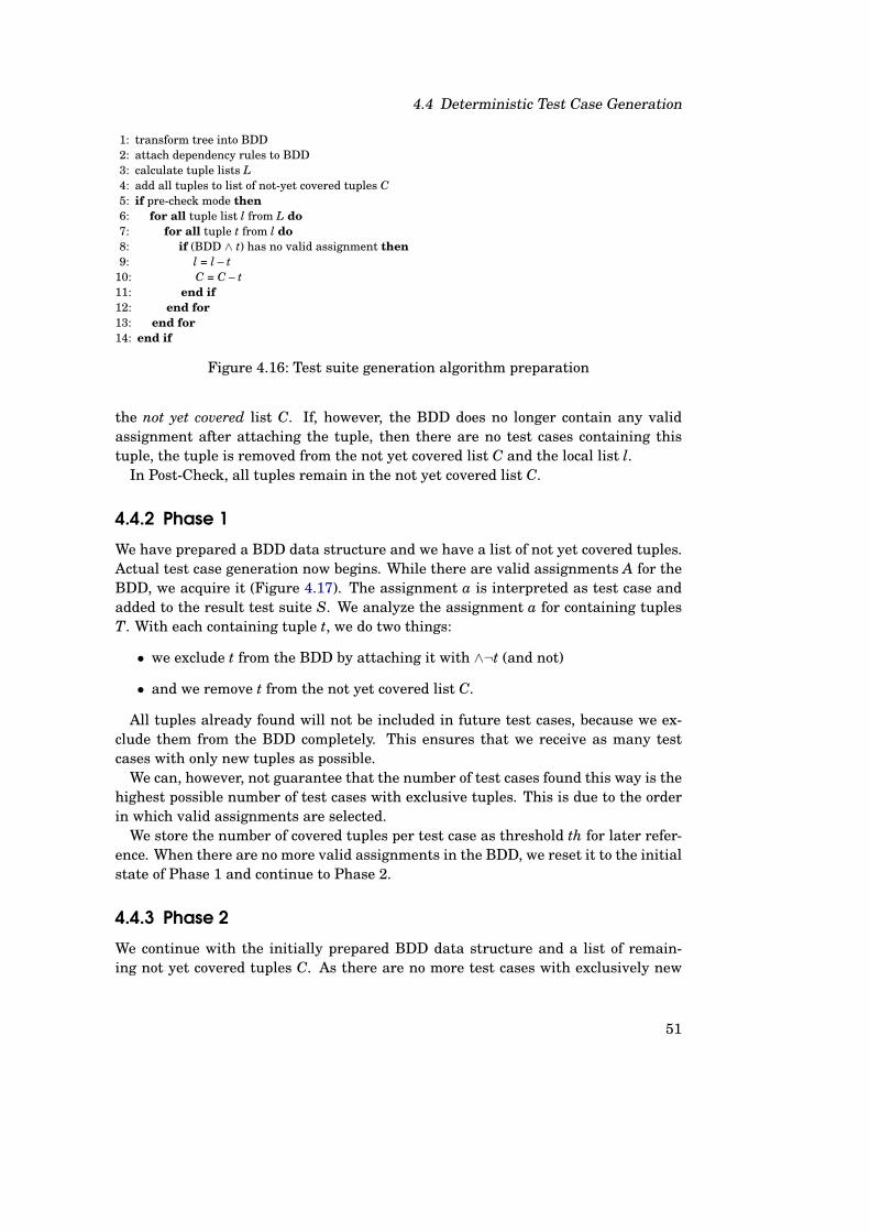
4.4 Deterministic Test Case Generation
1: transform tree into BDD2: attach dependency rules to BDD3: calculate tuple lists L4: add all tuples to list of not-yet covered tuples C5: if pre-check mode then6: for all tuple list l from L do7: for all tuple t from l do8: if (BDD ∧ t) has no valid assignment then9: l = l – t
10: C = C – t11: end if12: end for13: end for14: end if
Figure 4.16: Test suite generation algorithm preparation
the not yet covered list C. If, however, the BDD does no longer contain any validassignment after attaching the tuple, then there are no test cases containing thistuple, the tuple is removed from the not yet covered list C and the local list l.
In Post-Check, all tuples remain in the not yet covered list C.
4.4.2 Phase 1
We have prepared a BDD data structure and we have a list of not yet covered tuples.Actual test case generation now begins. While there are valid assignments A for theBDD, we acquire it (Figure 4.17). The assignment a is interpreted as test case andadded to the result test suite S. We analyze the assignment a for containing tuplesT. With each containing tuple t, we do two things:
• we exclude t from the BDD by attaching it with ∧¬t (and not)
• and we remove t from the not yet covered list C.
All tuples already found will not be included in future test cases, because we ex-clude them from the BDD completely. This ensures that we receive as many testcases with only new tuples as possible.
We can, however, not guarantee that the number of test cases found this way is thehighest possible number of test cases with exclusive tuples. This is due to the orderin which valid assignments are selected.
We store the number of covered tuples per test case as threshold th for later refer-ence. When there are no more valid assignments in the BDD, we reset it to the initialstate of Phase 1 and continue to Phase 2.
4.4.3 Phase 2
We continue with the initially prepared BDD data structure and a list of remain-ing not yet covered tuples C. As there are no more test cases with exclusively new
51

4 Enhancements
1: B = copy of BDD2: while BDD has valid assignment do3: a = get next assignment4: S = S + a5: T = get all tuples from a6: th = |T|7: for all tuple t from l do8: BDD = BDD ∧¬t9: C = C – t
10: L = L – t11: end for12: end while13: BDD = B // restore copy of BDD
Figure 4.17: Test suite generation algorithm for phase 1
tuples, we now try to fit in as many new tuples into a single test case as possible(Figure 4.18).
We select not yet covered tuples from list L and attach them to the BDD with ∧(Line 7).
To improve this process, we use tuples from the longest local lists L (Line 4), sowe prefer tuples from parameter combinations that have not been covered that muchyet.
We sort all tuples lists by their length and iterate trough them. We take the largestlist (Line 4) and go trough all tuples from it (Line 6). The tuple is then combinedwith tuples from all other lists (Line 15). In each step, we make a copy of the BDD byattaching the tuple to it using AND (Line 17). If now the BDD does not contain anyvalid assignments anymore, we cannot combine this tuple with previously selectedtuples. In Post-Check, we check this tuple against the original BDD and remove itnow if needed (Line 22). If the tuple is the last tuple and no other tuple fits, wecontinue with the BDD from the previous iteration. Otherwise we take the matchingtuple from the current list and continue with the new BDD (Line 20).
After combining all tuples from the largest list with other tuples, the BDD nowcontains a set of candidates (Line 31). The candidates consist of valid assignmentsfor the BDD for all tuples from the largest list of not yet covered tuples C. Whilethere are candidates W, we order the list by the number of contained new tuples n(Line 40) and drop candidates with less than threshold tuples th. We add the firstcandidate from the list to the result test suite S (Line 44), remove the tuples fromthe not yet covered list C and repeat.
We adapt the threshold when no candidate above the threshold has been found(Line 52). The new threshold is the minimum of either the reduced original thresholdor the number of tuples contained in the first candidate.
The algorithm stops, when all local lists are empty, either because all tuples areacovered by test cases or because tuples have been removed because they there areno valid test cases.
52

4.4 Deterministic Test Case Generation
1: candidates W2: while |C| > 0 do3: Sort tuples lists L by |ln|4: lmax = longest list from L5: B = copy of BDD6: for all tuple tmax from lmax do7: BDD = B ∧ tmax8: if post-check mode then9: if (BDD) has no valid assignment then
10: L = L – tmax11: C = C – tmax12: continue13: end if14: end if15: for all list l from L except lmax do16: for all tuple t from l do17: tempBDD = BDD ∧t18: if (tempBDD) has valid assignment then19: BDD = tempBDD20: continue21: else22: if post-check mode then23: if (BDD) has no valid assignment then24: l = l – t25: C = C – t26: end if27: end if28: end if29: end for30: end for31: W = W + valid assignments32: end for33: for all candidate w from W do34: if n < th then35: W = W – w36: end if37: end for38: m = |W|39: while |W| > 0 do40: Sort W by number of tuples t41: w = remove first element from W42: n = number of not yet tuples t in w43: if n >= th then44: S = S + w45: for all tuple t from w do46: C = C – t47: L = L – t48: end for49: end if50: end while51: if m = 0 then52: th = min (th*0.95, n)53: end if54: end while
Figure 4.18: Test suite generation algorithm for phase 2
53

4 Enhancements
4.4.4 Example
We will continue using the example from Section 4.1.1. During preparation, a BDDrepresenting the classification tree is calculated (Formula 4.10). In contrast to Sec-tion 4.2.3, we skip dependency rules here. We assume the generation rule to be:
pairwise(Vehicle, Speed, Daylight); (4.12)
The tuple lists L consists of three local lists l with l1 = PrecedingVehicle × Speed,l2 = PrecedingVehicle×Daylight, and l3 = Speed×Daylight.
There are 12 tuples in l1, eight tuples in l2 and six tuples in l3 (Table 4.11), result-ing in 26 tuples not yet covered in global list C. Since we do not use dependency rulesin our example, no checking for validity is required even in pre-check mode.
Table 4.11: Initial Tuple Listsl1 l2 l3
(Mot, low) (Mot, Day) (low, Day)(Mot, med) (Mot, Nit) (low, Nit)(Mot, hi) (Lim, Day) (med, Day)
(Lim, low) (Lim, Nit) (med, Nit)(Lim, med) (Cab, Day) (hi, Day)(Lim, hi) (Cab, Nit) (hi, Nit)
(Cab, low) (Tru, Day)(Cab, med) (Tru, Nit)(Cab, hi)(Tru, low)(Tru, med)(Tru, hi)
In Phase 1, the test suite S contains six test cases read from the BDD:
S ={(hi, Cab, Nit), (med, Cab, Day), (hi, Lim, Day),
(med, Lim, Nit), (low, Tru, Nit), (low, Mot, Day)}(4.13)
Since each test case consists of three tuples (e.g. a1 = (hi, Cab, Nit) consists of (Cab,hi), (Cab, Nit), and (hi, Nit)), the threshold th is set to 3.
Phase 2 starts with the eight tuples not yet covered in C (Table 4.12), with sixtuples from l1 and two tuples from l2.
The first set of candidates W is then calculated. The longest list with tuples is l1.All tuples t still in l1 are combined with tuples from l2, the only other remaining listwith tuples. The first candidate set W consists of:
W ={{(Mot, med), (Mot, Nit)}, {(Mot, hi), (Mot, Nit)}, {(Tru, med), (Tru, Day)},
{(Tru, hi), (Tru, Day)}, {(Cab, low)}, {(Lim, low)}}(4.14)
Since all candidates contain less tuples than the threshold th = 3, no candidate isadded to the resulting test suite S. Instead, the threshold is reduced to two, because
54
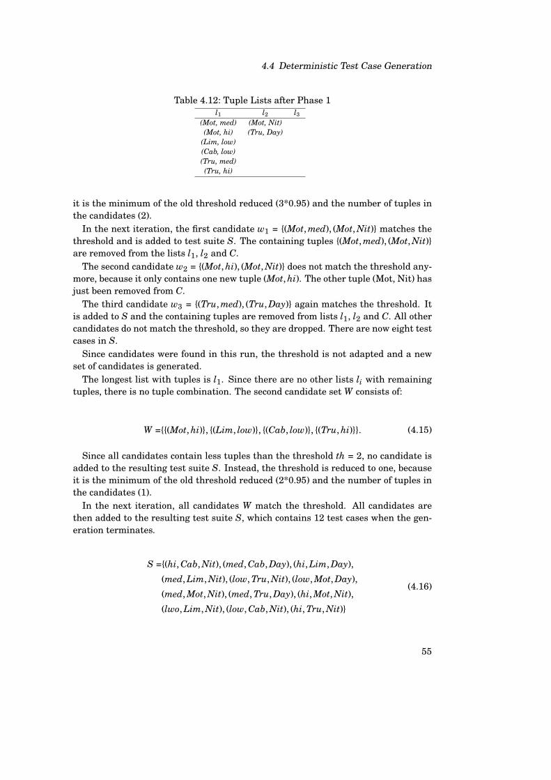
4.4 Deterministic Test Case Generation
Table 4.12: Tuple Lists after Phase 1l1 l2 l3
(Mot, med) (Mot, Nit)(Mot, hi) (Tru, Day)
(Lim, low)(Cab, low)(Tru, med)(Tru, hi)
it is the minimum of the old threshold reduced (3*0.95) and the number of tuples inthe candidates (2).
In the next iteration, the first candidate w1 = {(Mot, med), (Mot, Nit)} matches thethreshold and is added to test suite S. The containing tuples {(Mot, med), (Mot, Nit)}are removed from the lists l1, l2 and C.
The second candidate w2 = {(Mot, hi), (Mot, Nit)} does not match the threshold any-more, because it only contains one new tuple (Mot, hi). The other tuple (Mot, Nit) hasjust been removed from C.
The third candidate w3 = {(Tru, med), (Tru, Day)} again matches the threshold. Itis added to S and the containing tuples are removed from lists l1, l2 and C. All othercandidates do not match the threshold, so they are dropped. There are now eight testcases in S.
Since candidates were found in this run, the threshold is not adapted and a newset of candidates is generated.
The longest list with tuples is l1. Since there are no other lists li with remainingtuples, there is no tuple combination. The second candidate set W consists of:
W ={{(Mot, hi)}, {(Lim, low)}, {(Cab, low)}, {(Tru, hi)}}. (4.15)
Since all candidates contain less tuples than the threshold th = 2, no candidate isadded to the resulting test suite S. Instead, the threshold is reduced to one, becauseit is the minimum of the old threshold reduced (2*0.95) and the number of tuples inthe candidates (1).
In the next iteration, all candidates W match the threshold. All candidates arethen added to the resulting test suite S, which contains 12 test cases when the gen-eration terminates.
S ={(hi, Cab, Nit), (med, Cab, Day), (hi, Lim, Day),
(med, Lim, Nit), (low, Tru, Nit), (low, Mot, Day),
(med, Mot, Nit), (med, Tru, Day), (hi, Mot, Nit),
(lwo, Lim, Nit), (low, Cab, Nit), (hi, Tru, Nit)}
(4.16)
55

4 Enhancements
4.4.5 Variation
In this section, we present an approach for better variation of test case generation inPhase 1 and Phase 2.
Figure 4.19: Example for Generation without Variation
An example to illustrate the problem is given in Figure 4.19. It shows the expectedresult for the generation rule pairwise(A, B, E). Test cases 1 to 10 offer a good varia-tion on all classes of classifications references in the combination rule, A, B, and E.For the classifications C and D, there is no variation.
While this result is completely correct, it can be desirable to include some addi-tional variation on those classifications which do not offer new tuples to the test case.
A similar problem occurs when all tuples from a classification have been coveredduring test case generation and this classification is no longer under considerationfor new test cases.
Therefore, we propose the following solution: We apply variation onto all classes ofclassifications not being part of generation rules and to those classes not part of firsttime covering tuples.
The algorithm given in Figure 4.20 shows our approach.
1: for all selected class without influence on new coverage do2: get all (atomic) siblings3: select (deterministic) random sibling (can be original class again)4: if new testcase is valid then5: keep it6: else7: use original test case8: end if9: end for
Figure 4.20: Test Case Variation Algorithm
The algorithm inspects all tuples that do not have any influence on tuple coverage.
56
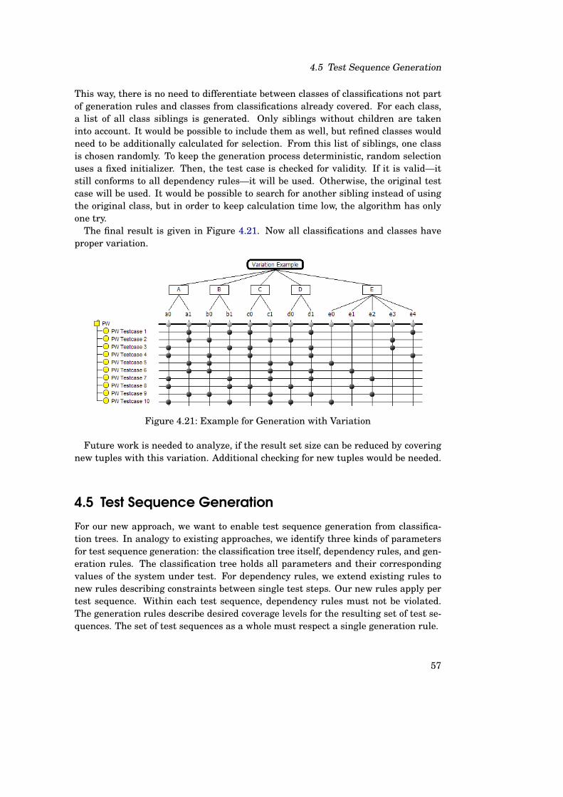
4.5 Test Sequence Generation
This way, there is no need to differentiate between classes of classifications not partof generation rules and classes from classifications already covered. For each class,a list of all class siblings is generated. Only siblings without children are takeninto account. It would be possible to include them as well, but refined classes wouldneed to be additionally calculated for selection. From this list of siblings, one classis chosen randomly. To keep the generation process deterministic, random selectionuses a fixed initializer. Then, the test case is checked for validity. If it is valid—itstill conforms to all dependency rules—it will be used. Otherwise, the original testcase will be used. It would be possible to search for another sibling instead of usingthe original class, but in order to keep calculation time low, the algorithm has onlyone try.
The final result is given in Figure 4.21. Now all classifications and classes haveproper variation.
Figure 4.21: Example for Generation with Variation
Future work is needed to analyze, if the result set size can be reduced by coveringnew tuples with this variation. Additional checking for new tuples would be needed.
4.5 Test Sequence Generation
For our new approach, we want to enable test sequence generation from classifica-tion trees. In analogy to existing approaches, we identify three kinds of parametersfor test sequence generation: the classification tree itself, dependency rules, and gen-eration rules. The classification tree holds all parameters and their correspondingvalues of the system under test. For dependency rules, we extend existing rules tonew rules describing constraints between single test steps. Our new rules apply pertest sequence. Within each test sequence, dependency rules must not be violated.The generation rules describe desired coverage levels for the resulting set of test se-quences. The set of test sequences as a whole must respect a single generation rule.
57

4 Enhancements
4.5.1 New Dependency Rules
Existing dependency rules allow the user to specify constraints between parametervalues of different parameters within one test case. With the new extended depen-dency rules, it will be possible to specify constraints between parameter values fromone test step to another. The following set of dependency rules will be supported(with i, j, k, n, o ∈ N; m ∈ Z):
• If class ci from classification C is selected in test step tn, then class cj fromclassification C must be selected in the succeeding test step tn+1.
• If C = ci in tn, then C = cj in a later tn+m.
• If C = ci in tn, then C = cj in all tn+1 to tn+m.
• If C = ci in tn, then C = cj in all tn+m to tn+o.
• Compositions of any (AND, OR, NOT, NAND, NOR, XOR, ...) combination, e.g.if C = ci OR B = bk in tn, then D = NOT dj in a later tn+m.
The existing dependency rules are a subset of our new dependency rules for tn andtn+m with m = 0.
Classic dependency rules are valid for manually created test cases, too. We wantour new dependency rules to be available for manually created test sequences, aswell.
4.5.2 New Generation Rules
Existing generation rules specify the coverage level of the resulting test suites. Forour new generation rules, we want to specify the following parameters:
• Desired coverage level.
• (Sub-)Set of all parameter-value combinations of the classification tree.
• Minimum and maximum number of test steps per test sequence.
• Set of special starting and ending parameter value combinations.
• Maximum number of test step repetitions (both local and global per resultingtest sequence).
• Maximum number of parameter value repetitions (both local and global perresulting test sequence).
58
4.5 Test Sequence Generation
4.5.3 General Approach
Ideally, the workflow should be as blackbox as possible. After a user has specified theclassification tree and all kinds of rules, the approach should work autonomically. Wedo, however, allow user interaction for advanced users to fine tune the results.
The input for test sequence generation consists of a common classification tree,a set of dependency rules and a single generation rule. Together, they are used togenerate an internal representation of the sequence generation problem. Then, a setof valid transitions and steps from one state in the internal representation to the nextone is defined, using the new dependency rules. This results in a set of all valid pathsthrough the internal representation. From this set some valid paths are selected tocreate subsets using the new generation rules. The output is then created by usingall remaining sequences.
This obviously leads to numerous sequences.Even for classical test case generation, it becomes crucial to select subsets from
the large set of possible test cases due to test case explosion. For classical test casegeneration, this can be done by both dependency rules and generation rules.
We identified decision trees and finite state machines as possible internal repre-sentations.
We decided to implement the new dependency rules using linear temporal logic(LTL) with the operators (X, G, F, U, R). LTL-terms fit well and fulfill most of therequirements defined in Section 4.5.1.
For generation rules, we used computation tree logic (CTL). CTL rules do not applyto single sequences but refer to the whole set of generated test sequences.
Additionally, we need some approach-specific rules. In state machines, we want tolimit the number of cycles. For decision trees, this setting is not needed. All otherneeds in generation rules not addressed by CTL will be called approach-specific rules.
The set of valid states consists of the set of all valid test cases, which can alreadybe very large. Therefore, the user starts with the generation of classical test casesand can use them as a subset of all valid test cases for the remaining test sequencegeneration.
The transitions of all states are then restricted by the dependency rules, generationrules and approach-specific rules. If no dependency rules are given, all transitionsare valid in our approach. A transition remains valid as long as there is no contradict-ing dependency rule. One could, however, define the opposite way: Only transitionsspecified in dependency rules are allowed whereas transitions not mentioned in orcontradicted by dependency rules could be removed.
After removing all forbidden transitions, a set of valid passes through the internalrepresentation remains. By applying generation rules and approach-specific rules,we now select a subset. The approach-specific rules can, for example, limit the pathlength, the number of cycles or the desired coverage level.
The output is a set of test sequences. Together, they fulfill the single generationrule and approach-specific rules, either one fulfills the dependency rules.
59

4 Enhancements
We have initially implemented the generation of test sequences using decisiontrees and finite state machines. Both approaches follow a simple work flow.
Generation input includes the classification tree, a set of dependency rules and gen-eration rules. For all approaches under evaluation, these three components should begeneric. A test suite of test sequence is the output of the generation of test sequences.The actual test sequence generation can be divided into four steps: The derivationof nodes, the definition of valid transitions between these nodes, the composition ofvalid paths (containing these transitions), and the selection of a subset of all possiblepaths. The actual generation might need additional approach-specific rules.
4.5.4 Decision Tree Approach
For the decision tree approach, the work flow is as follows: The nodes contain all pos-sible combinations of classes from the classifications. The number of nodes equals thesize of the complete coverage, the Cartesian product of all classes from all classifica-tions of the tree. Only valid nodes—containing valid class combinations—are addedto this set. In this step, all conventional dependency rules and implicit dependenciesare handled. For this set, all valid transitions are generated. The dependency rulesare applied, where possible. Only those rules describing constraints between consec-utive test steps can be processed. From this set of simple transitions, between twonodes each, a decision tree is then composed. Here, all still unprocessed dependencyrules are taken into account. The resulting decision tree now contains both all validpaths and only valid paths. In the last step, a path selection is made to fulfill thegeneration rule. We developed two approaches here, a brute-force and a random ap-proach. The brute-force approach starts traversing the decision tree in a depth firstsearch. When reaching an atomic node in the tree, the path is added to the resultset. When reaching a node, which will not reach anything new, this path is skipped.The random approach randomly selects complete paths from the decision tree. Bothapproaches stop as soon as the generation rule is complete.
4.5.5 FSM Approach
For a given classification tree, the user must specify a set of valid LTL rules. Therules are then used to build a Büchi automaton using Formula Rewriting, Core Trans-lation and actual Automaton Generation following an algorithm [GPV+95] which usesa Tableaux Construction Method for LTL given in [CGP99, p. 132]. The Büchi au-tomaton is then reduced to a regular FSM by removing all infinite properties usingweak Next- (and Until-) Operators in Finite Trance LTL and excluding empty se-quences. The FSM is then converted into a Test Case FSM by identifying possibletest case candidates for each state and removing states without valid test cases. TheTest Case FSM can then be traversed with different coverage levels: State Coverage(C0), Transition Coverage (C1) and Path Coverage (C2).
The search for a minimal State Coverage is equivalent to the search for a Hamiltonpath in a directed graph [Sed03, p. 60]. The search for a minimal Transition Coverage
60

4.6 Statechart Approach for Test Sequence Generation
is equivalent to an asymmetric Traveling Salesman Problem [Pun04]. Both searchesare known to be NP-complete. The search for a minimal Path Coverage is equivalentto the search for an Euler path [Sed03, p. 62] or in some cases the Chinese PostmanProblem [Sed03, p. 224].
Only Path Coverage has been implemented, a depth first search uses an Adjacencymatrix that allows specifying the minimum and maximum search depth (equivalentto the resulting path length) and the minimum and maximum number of state repe-titions.
4.6 Statechart Approach for Test Sequence Generation
We will first introduce the refined requirements for the generation rules and thenintroduce the actual approach.
It can be desirable to have specific coverage levels and it can be useful to generatea test suite with test sequences covering all possible transitions between classes ofthe classification tree.
4.6.1 New Generation Rules
In analogy to conventional test generation, covering all pairs of transitions betweenclasses of the classification tree could be defined as well. Conventional test casegeneration supports mixed strength generation as well as seeding [CDFP97], so werequire them as well.
New generation rules should allow any t-wise coverage for both classes and tran-sitions. Note that some of Kuhn’s t-way sequences [KKL10] can be mapped onto ourgeneration rules.
Kuhn’s 1-way sequence coverage corresponds to 1-wise (or minimal) class coveragehere. Each class is supposed to be contained in the result set at least once. Ourapproach extends conventional class coverage for test cases to test sequences.
Kuhn’s 2-way sequence coverage corresponds to our 1-wise (or minimal) transitioncoverage. All valid transitions (pairs of states) are supposed to be contained in theresult set at least once. In conventional test case generation, there is no coveragecriterion for transitions.
Higher n-way (with n > 2) sequence coverage is not yet included and requiresfuture work. Instead, we require higher n-wise (with n > 1) coverage for both classesand transitions. We have included pairwise class and transition coverage.
The generation rules should take classifications as parameters to specify their fo-cus. The number of parameters should not be restricted. Elements of generationrules should be combinable to allow mixed strength generation. Seeding [CDFP97]of manually created test sequences should be possible. The generation algorithmshould then analyze this set and take these sequences into account. The generationshould, of course, take the dependency rules into account.
61
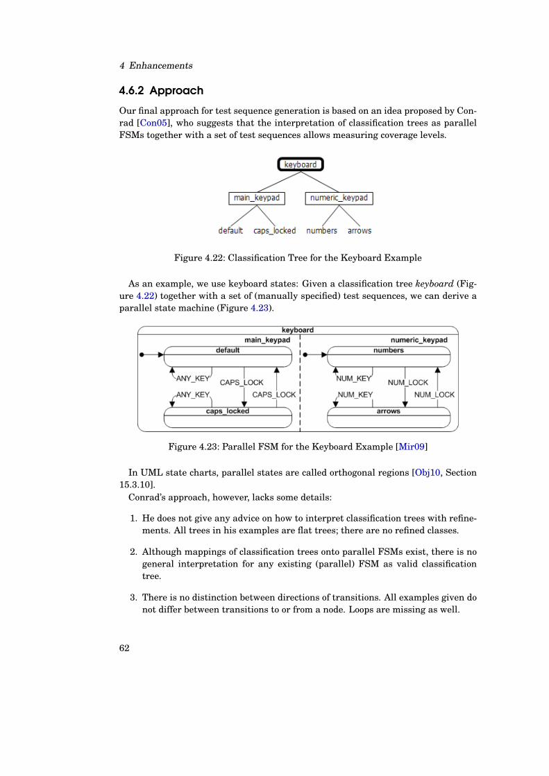
4 Enhancements
4.6.2 Approach
Our final approach for test sequence generation is based on an idea proposed by Con-rad [Con05], who suggests that the interpretation of classification trees as parallelFSMs together with a set of test sequences allows measuring coverage levels.
Figure 4.22: Classification Tree for the Keyboard Example
As an example, we use keyboard states: Given a classification tree keyboard (Fig-ure 4.22) together with a set of (manually specified) test sequences, we can derive aparallel state machine (Figure 4.23).
Figure 4.23: Parallel FSM for the Keyboard Example [Mir09]
In UML state charts, parallel states are called orthogonal regions [Obj10, Section15.3.10].
Conrad’s approach, however, lacks some details:
1. He does not give any advice on how to interpret classification trees with refine-ments. All trees in his examples are flat trees; there are no refined classes.
2. Although mappings of classification trees onto parallel FSMs exist, there is nogeneral interpretation for any existing (parallel) FSM as valid classificationtree.
3. There is no distinction between directions of transitions. All examples given donot differ between transitions to or from a node. Loops are missing as well.
62

4.6 Statechart Approach for Test Sequence Generation
4. His approach does not handle dependencies. The test engineer has to decide onhis own, which combination of classes and which order of consecutive test stepsare valid.
5. There is (to the best of our knowledge) no automatic test sequence generation inConrad’s approach. The test engineer has to specify all test sequences manually.
We will now handle these short comings one by one:
1. The interpretation of refined classes can be easily accomplished by mappingthem on to hierarchical states in state machines. This concept is known fromHarel statecharts [Har87] as well. As in classification trees, statecharts can bemodeled top-down, from overview to detail, by refining states with a set of sub-states. This allows different levels of granularity within a single statechart atdifferent hierarchies. Parallel FSMs are sometimes also known as HierarchicalConcurrent finite State Machine (HCSM) [Luc93]. We will from now on callConrad’s approach, the statechart approach.
2. Conversion of existing statecharts to classification trees will be explained in thenext section (Section 4.6.3).
3. We will differentiate between different transition directions and will enforceloop transitions (transitions where start-node and end-node are the same), ifthey exist.
4. For handling dependencies, we will use our own initial dependency rule ap-proach for test sequence generation. To have only one central dependency han-dling, we will model transition guards using this technique as well.
5. The actual test sequence generation will be given in detail in Sections 4.6.4 and4.6.5.
4.6.3 Conversion of Existing Statecharts to Classification Trees
To illustrate the problem, we will borrow the example from [Luc93].The microwave (Figure 4.24) is a good example because it contains concurrency
and hierarchies.We propose the following classification tree (Figure 4.25) as an equivalent repre-
sentation.
63

4 Enhancements
Figure 4.24: Statechart for the Microwave Example
Figure 4.25: Classification Tree for the Microwave Example
64
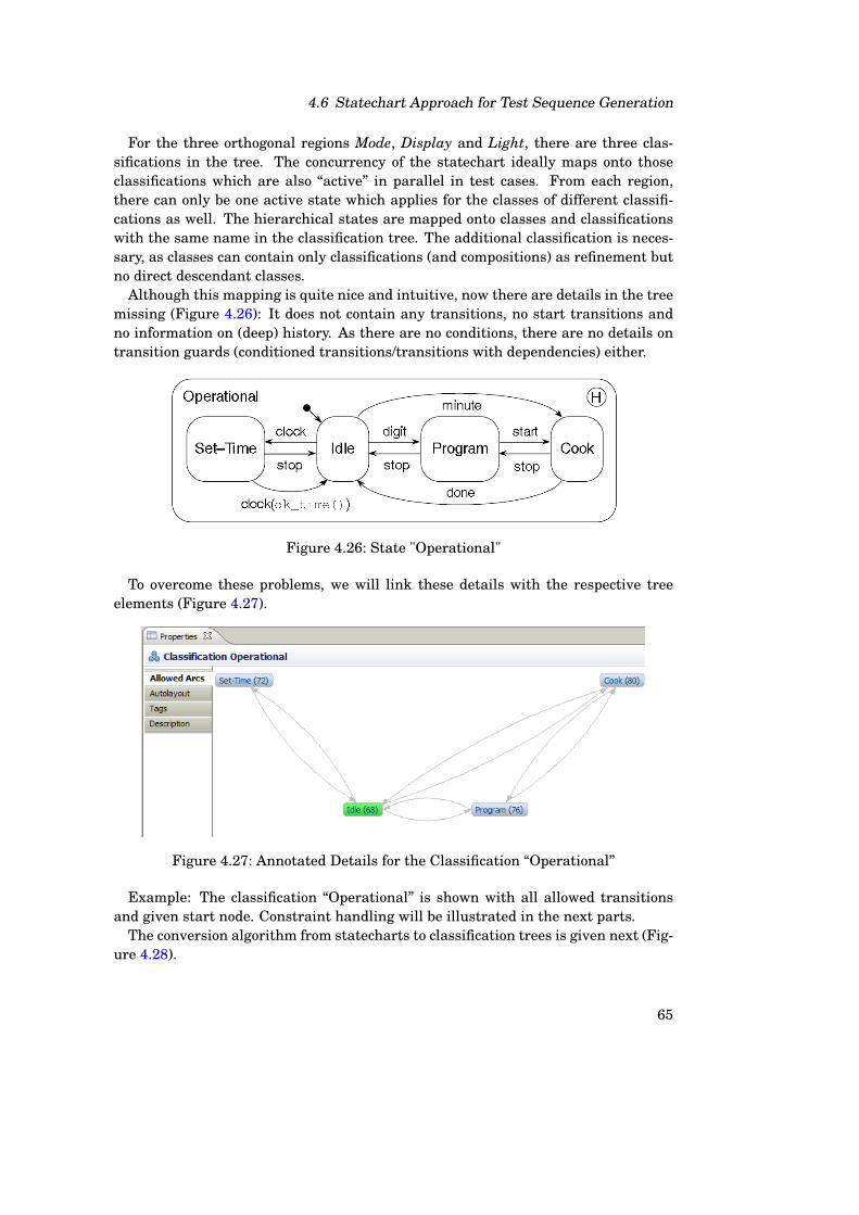
4.6 Statechart Approach for Test Sequence Generation
For the three orthogonal regions Mode, Display and Light, there are three clas-sifications in the tree. The concurrency of the statechart ideally maps onto thoseclassifications which are also “active” in parallel in test cases. From each region,there can only be one active state which applies for the classes of different classifi-cations as well. The hierarchical states are mapped onto classes and classificationswith the same name in the classification tree. The additional classification is neces-sary, as classes can contain only classifications (and compositions) as refinement butno direct descendant classes.
Although this mapping is quite nice and intuitive, now there are details in the treemissing (Figure 4.26): It does not contain any transitions, no start transitions andno information on (deep) history. As there are no conditions, there are no details ontransition guards (conditioned transitions/transitions with dependencies) either.
Figure 4.26: State "Operational"
To overcome these problems, we will link these details with the respective treeelements (Figure 4.27).
Figure 4.27: Annotated Details for the Classification “Operational”
Example: The classification “Operational” is shown with all allowed transitionsand given start node. Constraint handling will be illustrated in the next parts.
The conversion algorithm from statecharts to classification trees is given next (Fig-ure 4.28).
65

4 Enhancements
1: create rootNode with Name of statechart2: readState (statechart, rootNode)3:4: readState(state, treeItem)5: if state is concurrent then6: for all for each partition do7: create a classification with name of partition8: readChildren (partition, classification)9: end for
10: else11: // state is non-concurrent12: create classification with name of parent state13: readChildren (state, classification)14: end if15:16: readChildren (state, classification)17: if state has history then18: classification set history (true)19: end if20: for all child of state do21: create one class22: readState (child, classification) // recursion23: if child is start then24: classification add start (child)25: end if26: for all transition of child do27: classification add transitions (transition)28: end for29: end for
Figure 4.28: Statechart to Classification Tree Algorithm
First, the root node of the tree is named after the state machine. The readState-method is then called with both the current state, which is the state machine itselffor the first call, and the current tree item, in this case the root node. The readState-method basically differs only between concurrent and non-concurrent states (Line 5).For concurrent states, it creates a classification for each partition with the name ofthis partition (Line 7). All children are then added to the corresponding classifica-tion. For non-concurrent states, a new classification with the name of the parentstate is added, resulting in a classification with the same name as its parent treeitem (Line 12). Children of non-concurrent states are then added to this single clas-sification.
The readChildren-method first checks whether the state has a (deep) history andstores this information in the corresponding classification. For each child of the state,it creates a class element in the classification tree (Line 21). Each child is then re-cursively processed by calling the readState-method. If one of the children is markedas start state (it has a start transition), it is added to the list of possible start statesin the parent classification. All outgoing transitions of each child are also stored inthe classification.
66

4.6 Statechart Approach for Test Sequence Generation
In contrast to an earlier approach [HHS03], we can read more details from theformal specification. This way, information on model internals such as constraintsand transistions can be preserved when building the classification tree, reducingmanual work by the tester. The additional details will then be used for the actualtest sequence generation (Section 4.6.5).
4.6.4 Conversion of Classification Trees to Statecharts
For the actual test sequence generation from classification trees, we make some de-fault assumptions:
• In any given plain classification tree, there are no transitions between classes,resulting in an unconnected graph. Test sequence generation will lead to se-quences with only one single test step. These test suites are similar to conven-tional test case generation. Transition coverage is, of course, not available.
• We allow all classes to be reached at start.
• Classifications do not have a (deep) history.
The conversion algorithm from classification trees to statecharts is given next (Fig-ure 4.29).
The build-method takes a tree item as the input parameter and returns its cor-responding state machine. First, a list of child states is prepared by recursivelybuilding all children of the current tree item.
The build-method then distinguishes between several cases: If the current treeitem is a class or a composition (Line 9), it distinguishes again between the number ofchildren. If a class or a composition has more than one child (Line 10), then this treeitem is a parallel state and all children are partitions of it. If a class or a compositionhas exactly one child (Line 22), it is skipped by directly adding all the child’s childrento the current tree item. In all other cases, e.g. the tree item is a class or a compositionwithout any children or the tree item is a classification, the prepared list of childrenis used as the result’s list of children (Line 28).
All transitions and possible start states stored in the classification are read andthe result is returned.
4.6.5 Algorithm
The algorithm takes the first and second step of our generally defined workflow. Thenodes are the classes and classifications from the classification tree. Simple refine-ment classifications are skipped. Valid transitions can directly be parsed from theannotation in the tree. For the last two steps of the work flow, we propose the follow-ing solution.
We use two phases and two kinds of agents to traverse the tree. Travelling is donein such a manner that only valid paths are taken and that all travelled paths togetheralready result in the desired coverage so that there is no need for subset selection.
67
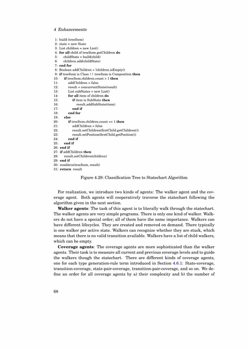
4 Enhancements
1: build (treeItem)2: state = new State3: List children = new List()4: for all child of treeItem.getChildren do5: childState = build(child)6: children.add(childState)7: end for8: Boolean addChildren = !children.isEmpty()9: if treeItem is Class || treeItem is Composition then
10: if treeItem.children.count > 1 then11: addChildren = false12: result = concurrentState(result)13: List subStates = new List()14: for all item of children do15: if item is SubState then16: result.addSubState(item)17: end if18: end for19: else20: if treeItem.children.count == 1 then21: addChildren = false22: result.setChildren(firstChild.getChildren())23: result.setPosition(firstChild.getPosition())24: end if25: end if26: end if27: if addChildren then28: result.setChildren(children)29: end if30: readArcs(treeItem, result)31: return result
Figure 4.29: Classification Tree to Statechart Algorithm
For realization, we introduce two kinds of agents: The walker agent and the cov-erage agent. Both agents will cooperatively traverse the statechart following thealgorithm given in the next section.
Walker agents: The task of this agent is to literally walk through the statechart.The walker agents are very simple programs. There is only one kind of walker. Walk-ers do not have a special order; all of them have the same importance. Walkers canhave different lifecycles. They are created and removed on demand. There typicallyis one walker per active state. Walkers can recognize whether they are stuck, whichmeans that there is no valid transition available. Walkers have a list of child walkers,which can be empty.
Coverage agents: The coverage agents are more sophisticated than the walkeragents. Their task is to measure all current and previous coverage levels and to guidethe walkers though the statechart. There are different kinds of coverage agents,one for each type generation-rule term introduced in Section 4.6.1: State-coverage,transition-coverage, state-pair-coverage, transition-pair-coverage, and so on. We de-fine an order for all coverage agents by a) their complexity and b) the number of
68

4.6 Statechart Approach for Test Sequence Generation
parameters, which is the number of scopes they cover. The lifecycle of the coverageagents start with the beginning of the generation process. They remain active un-til the coverage criterion they handle is finished. There is one coverage agent pergeneration rule term/component, e.g. the rule
state-pairwise(a, b) + transitions(a, b, c)
results into two coverage agents.Coverage agents can determine whether they are finished, both globally and lo-
cally. From the example above, we can explain complexity and number of parametersneeded for ordering the coverage agents. We use the following formula to calculatethe order of coverage agents:
i = |order|*|parameters|
If two terms have the same index value, we will prefer the term being early in thegeneration rule formula which can result into missing commutative property for cer-tain generation rules.
Walker algorithm: The basic idea of the algorithm (Figure 4.30) is that all walk-ers will, one by one, ask the most complex remaining coverage agent where to go next.By walking the route proposed by the most complex coverage agent first, chances arehigh to cover elements needed by simpler coverage agents, too. For example, transi-tion coverage for a statechart already implies state coverage, too.
The very first step is the creation of coverage agents from the generation rule.Then, the root node (statechart) is selected. This means, a walker is created for theroot node. For each classification (parallel section) under the root node, the class(node) with the start transition is selected (Lines 4-9). There will consequently beone walker per classification now. The selection of start nodes is repeated as long asa selected class (state) has at least one refinement (inner states). A new walker isthen created for each refinement step and will be added to the list of child walkers.
As soon as all walkers without child walkers reach an atomic class, the first teststep is created. This test step is then checked against the conventional dependencyrules. If it is valid, then the test step is added to the test sequence (Line 12) andthe coverage measure is updated (Line 13). If it is invalid, test sequence generationis canceled and an empty result set is given (Line 15) as there are no valid testsequences available from this specification.
As long as generating, each walker without child walkers will now perform thefollowing steps. It first identifies (Line 20) the most complex remaining coverageagent. It will then ask this agent where to go next or to stay (Line 21). The candidateclass is then checked against conventional and new dependency rules together withall walkers already moved in this turn. If the candidate is valid, we continue withthe next walker until all walkers have walked. We then add this test step to thetest sequence (Line 32) and update the coverage. We then start the next turn ofwalking walkers. If the candidate node does not offer any valid test step, the walkerwill take the second best move from the coverage agent candidates and validates it
69

4 Enhancements
again until a valid test step candidate is found. If all candidates fail, the walkerwill try to stay where it is. If that is not possible, it can still try to step out, whichmeans, its parent walker will move. If even that is not an available option, we startbacktracking (Line 35).
1: create coverage agents from rule2: select root node // statechart3: create walker4: for all classification // parallel section do5: repeat6: select (inner) start class // node7: create walker, add to walker child list8: until class is atomic9: end for
10: compose test step from selected classes11: if valid then12: add test step to sequence13: update coverage14: else15: cancel generation with empty results16: finished = true17: end if18: while not finished do19: for all walker without child-walker do20: find coverage agent21: ask coverage agent where to go or stay22: decide if stuck23: if walk transition then24: while entering a refined class do25: select (inner) start class26: create walker, add to walker list27: end while28: end if29: end for30: compose test step from selected classes31: if valid then32: add step to sequence33: update coverage34: else35: backtracking36: end if37: end while
Figure 4.30: Test Sequence Generation Algorithm, Phase 1
The candidate from the previous walker is rejected now and the next best choicefrom this previous walker is taken. This is done recursively until one valid candidatecan be found. If there is no candidate—the first walker does not find a valid option—the statechart is globally stuck. It will be reset to its initial state by turning it offand on again.
If adding test steps to the test sequence does not increase coverage for a certainnumber of steps, we will reset the statechart, as well, and start a new test sequence.
70

4.6 Statechart Approach for Test Sequence Generation
We wait as many steps as there are (inner) classes in the largest classification. Allsteps without progress are removed from the sequence before adding it to the resulttest suite.
We repeat this until the global coverage is completed or resetting and starting anew sequence does not increase coverage for a certain number of test sequences; thenwe can stop. We again wait as many test sequences as there are (inner) classes inthe largest classification. In this case, we start a second phase for hard to reachconfigurations.
Second phase: The algorithm for the second phase for hard to reach configurationis given in Figure 4.31. The approach is inspired by [GFL+96].
1: for all coverage agent (in descending order of importance) do2: for all not yet covered item do3: find path from item to start in a reverse breadth first search4: if there is valid path then5: add test sequence of path to result set6: else7: drop item from coverage measure8: end if9: end for
10: end for
Figure 4.31: Test Sequence Generation Algorithm, Phase 2
The approach is rather simple here. For all coverage agents we get all not yetcovered items. We apply a reverse breadth first search for paths from this item topossible start states (Line 3). If a valid path is found, it is added to the result set(Line 5). If there is no valid path, the item is not reachable and is dropped (Line 7).
The approach guarantees the coverage of all coverable items. The result set, how-ever, might not be minimal.
Coverage algorithm: The rating algorithm works as follows (Figure 4.32). It getsa candidate state or transition. For state coverage, self transitions are ignored andzero is returned. Otherwise, it then adds this candidate to a queue together with aweight factor, with an initial weight factor of one. The initial rating is set to zero.The candidate is added to the list of rated items. Then while the queue is not emptythe algorithm polls the next state and weight factor from the queue. If the pollednode is the original candidate and if the rating is larger than zero, the algorithm hasfound a loop path with new items. This loop path is preferred by adding the value of100 to the rating. In this case, or when the current item is on the list of rated items,the while loop goes to its next cycle. Else this node is added to the list of rated items.If the node is on the list of target states (it has not been used in any test step before),the algorithm adds 10 times the weight factor to the result rating. Then, if there areoutgoing transitions, child nodes, or subsections, the weight factor is multiplied witha punishment value of 0.95. Target states of outgoing transitions, child nodes andsubsections are then added to the queue together with the new weight factor. Whenthe queue is empty the rating is returned.
71

4 Enhancements
1: candidate state or transition2: if state coverage && self transition then3: return 04: end if5: weight = 1.06: rating = 07: queue += (candidate, weight)8: while !queue.empty do9: (item, weight) = queue.poll
10: if item == candidate && rating > 0 then11: rating += 10012: continue13: end if14: if ratedItems contains then15: continue16: end if17: ratedItems += item18: if targetNodes contains item then19: rating += 10 * weight20: end if21: if item has (outgoing transition || childnodes || subsections) then22: weight *= 0.9523: end if24: for all (outgoing transition && childnodes && subsections) of item do25: queue += (item, weight)26: end for27: end while28: return rating
Figure 4.32: Rating of Candidates
For pairwise coverage, the rating algorithm needs to take into account all walkersat once. When rating moves for state pairwise, the rating algorithm uses two lists,one containing all positions of walkers which will be moved and one list of positionsof walkers that have already been moved in this turn. It sends walkers one at a timeto states that cover state pairs together with all walkers in the statechart.
For transition pair coverage, the rating algorithm uses a list of all transitions al-ready taken in a move together with the list of positions of walker which still canmove during this turn. The rating algorithm then sends walkers through the state-chart in such a manner that joint moves of walkers cover transition pairs.
The remaining part of the pair rating works just like the rating of states and tran-sitions.
72

5 Evaluation
After designing and implementing our approaches, we evaluate them in this chapter.We first apply a prioritized benchmark to both the prioritized pairwise combinationand the plain pairwise sorting approach (Section 5.1). We then apply a large set ofstandard benchmarks to our new deterministic test case generation approach (Sec-tion 5.2). We introduce a set of case studies for test sequence generation and evaluateour new test sequence generation approach (Section 5.4).
5.1 Prioritized Generation
Here, we evaluate the impact of weight consideration on weight coverage and on theabsolute size of the generated test suites. A first impression is given in Figure 5.1.
Weight Covered using plain pairwise, PCC and sorting
0%
20%
40%
60%
80%
100%
120%
1 2 3 4 5 6 7 8 9 10 11 12Test Number
Cum
ulat
ive
Wei
ght C
over
ed
PPCSortingNon-weighted
Figure 5.1: Comparison of PPC, Sorting, and of Non-Weighted Generation
The Figure shows a comparison of PPC, Sorting and a non-weighted generation forthe the ACC example using the usage model. As can be seen, PPC and sorting per-form similar while the unsorted test suite does not perform that well. For a more de-tailed and systematic evaluation, we use the set of benchmarks proposed in [BC06]:We compare (1) our PPC approach with our sorting approach and (2) PPC with the
73

5 Evaluation
deterministic density algorithm (DDA) given in [BC06]. The given benchmark usesfour different weight distributions applied to eight scenarios. The distributions are:
• d1 (Equal weights)—All levels have the same weight.
• d2 (50/50 split)—Half of the weights for each factor are set to 0.9, the otherhalf to 0.1.
• d3 ((1/vmax)2 split)—All weights of levels for a factor are equal to (1/vmax)2
where vmax is the number of levels associated with the factor.
• d4 (Random)—Weights are randomly distributed.
The scenarios s1, ..., s8 with their resulting test suite sizes are given in Table 5.1.The factors are given in a shorthand notation, for example s5 with 82726224 consistsof 2 factors with 8 values, 2 factors with 7 values, 2 factors with 6 values, and 4factors with 2 values. The columns d1, ..., d4 provide the different results for the PPCruns. The sort column reports the resulting test suite size for the sorting approachregardless of the distribution.
Table 5.1: Benchmark Scenarios Result SizesFactors d1 d2 d3 d4 sort
s1 34 10 12 10 12 9s2 1020 218 228 218 229 245s3 3100 130 51 130 52 34s4 1019181716151413121 92 100 109 106 94s5 82726224 71 78 86 80 74s6 1511055141 172 190 177 187 177s7 350250 70 42 84 33 29s8 2021023100 400 403 420 404 400
5.1.1 Comparison of PPC vs. Sorting
Size. The test suites generated using the PPC are larger than those generated usingthe sorting approach (Table 5.1). The PPC-generated scenarios s3 and s7 in d1 and d3are up to 300% larger than their sorting counterparts. The problem here seems to bethe combination of scenario and distribution. For any other distribution or scenario,the PPC results are much smaller and, therefore, closer to the sorting results. Forthe rest, the resulting PPC test suites are up to 50% larger in some cases (s3 d4 ors7 d2). On average, the PPC test suites are 42% larger than the sorting test suites.Ignoring the extreme values (s3 and s7 from d1 and d3), the PPC test suites are 12%larger on average.
Applying equal sorting (d1), the PPC algorithm results in smaller test suites forsome scenarios. For s2, it is generally smaller. The normal test case generationserving as input for the test case sorting seems to have problems with this particular
74

5.1 Prioritized Generation
scenario. To reveal the reasons behind this behavior, further investigation is needed.For s6 d3, the PPC test suite has the same size as the sorting.
For the majority of scenario-distribution combinations, sorting results in smallertest suites, which is not surprising since in prioritization selection focuses on classweights first; in contrast to sorting, which tries to get the smallest test suite avail-able.
Weight coverage. The detailed results are given in Table 5.2. The first columngives the desired weight. The second column gives the scenario. The remaining fourcolumns give the number of test cases needed to reach the weight for each distribu-tion. The values for both algorithms, PPC and sorting, are given next to each otherwith the smaller value highlighted in bold font.
In d1, sorting starts very strong. Reaching 25% coverage is always better than orequal to PPC. For 50% and 66%, PPC is only better in s2 where sorting seems to havea general weakness, and s8. For the rest of measured weights, PPC becomes betterand better, while sorting loses its advantages from the lower values.
In d2, the prioritization performs better in all scenarios for the 25%–75% targetweights. Starting at 90%, sorting gets better with s1 and s8. For 95%, sorting alsoneeds fewer test cases with s4. This case needs further investigation, maybe it is justa good weight distribution for the test case generator creating the PPS input. For99%, sorting only performs best for s1.
In d3, sorting comes close to the PPC. For 25% coverage, both approaches performequally. For 50%, the PPC is only better for s2 and s7. For 66% weight coverage, theprioritization is better for s2, s4, s6, and s8. For 75% coverage, PPC is always betterfor large scenarios (s2, ..., s7). For 90% and 95% coverage, sorting performs equallyboth for s7 and s3 for the latter. For 99% coverage, sorting surpasses PPC for half ofall scenarios.
In d4, the prioritization approach provides the best weight coverage. Random dis-tribution of weights leads to a high weight coverage when performing test case com-position with its pair selection.
In general, the PPC gives better weight coverage. There are, however, three excep-tions: Very small scenarios, problematic distributions, and very high weight marks.For very small scenarios, sorting has a good starting point since any pairwise-coveringtest suite has a good chance for containing combinations of any class pair, even com-binations of only high-weight pairs. In these cases, sorting can sort the good combi-nations to the beginning. The influence of problematic distributions has already beenanalyzed in detail earlier. PPC performs better on random and (1/vmax)2 split whileit has some problems on equal distributions (with low target covering marks) and ison par with the sorting approach on the 50/50 split. For higher target marks on equaldistributions, it becomes better again since sorting has a general problem here. Forvery high weight marks starting at coverage around 95% or 99% or even higher, PPCloses its advances gradually. Since sorting performs better for 100% coverage, thereobviously must be a point ≤ 100% where both approaches perform equally.
To conclude. Having two algorithms which both generate test suites covering all
75

5 Evaluation
Table 5.2: Benchmark Detailed Resultweight d1 d2 d3 d4
25% s1 3 3 1 1 3 3 2 2s2 27 27 9 12 27 27 12 19s3 3 3 1 2 3 3 1 3s4 11 10 3 4 4 4 6 7s5 8 7 2 3 2 2 3 4s6 23 22 7 9 12 12 11 14s7 2 2 1 2 2 2 1 2s8 3 3 1 1 3 3 2 3
50% s1 5 5 1 2 5 5 3 3s2 56 60 18 36 56 60 31 47s3 6 6 1 4 6 6 3 5s4 24 22 8 11 8 8 15 18s5 18 17 6 8 4 4 8 10s6 52 49 17 24 26 26 27 36s7 4 4 1 3 3 4 2 4s8 8 9 3 3 6 6 5 8
66% s1 7 6 1 3 7 6 5 5s2 79 89 27 60 79 89 50 74s3 8 8 1 7 8 8 5 8s4 36 34 12 17 12 14 23 28s5 28 27 10 15 7 7 14 17s6 74 74 25 39 38 41 43 57s7 6 6 1 4 5 5 4 6s8 13 15 7 8 8 9 10 15
75% s1 8 7 3 4 8 7 6 5s2 95 110 36 79 95 110 65 95s3 9 10 4 8 9 10 7 10s4 45 42 16 23 16 19 29 36s5 35 34 13 21 9 10 19 24s6 89 92 31 53 46 53 56 73s7 7 8 2 5 6 7 5 7s8 18 21 12 13 9 11 15 21
90% s1 9 9 7 5 9 9 8 7s2 132 162 87 131 132 162 104 150s3 15 16 9 13 15 16 12 15s4 64 63 36 38 30 35 46 56s5 50 51 28 37 15 19 33 41s6 123 131 73 92 83 92 90 111s7 11 12 6 9 10 10 9 11s8 64 46 30 30 15 19 35 43
95% s1 10 9 8 7 10 9 10 8s2 152 190 121 163 152 190 129 181s3 20 20 12 16 20 20 15 19s4 74 74 53 51 42 46 59 67s5 57 59 43 46 23 25 44 50s6 139 149 106 114 107 120 112 131s7 14 15 9 12 13 13 11 14s8 92 62 56 47 19 26 55 60
99% s1 10 9 11 8 10 9 11 9s2 180 228 169 212 180 228 169 223s3 37 26 19 23 37 26 21 26s4 86 88 76 77 72 70 82 82s5 66 68 61 62 52 54 60 65s6 159 169 148 153 149 158 148 160s7 20 21 14 18 21 19 17 21s8 145 120 114 122 28 45 120 13776

5.1 Prioritized Generation
possible pair combinations, the PPC covers weights better than the sorting approachbecause it tries to combine high weight pairs into early test cases. The sorting ap-proach is worse because it has no influence on the actual composition of test caseswith their contained pairs. So while both test suites contain all possible class pairs,PPC results in early weight coverage.
5.1.2 Comparison of PPC with DDA
Size. Comparing PPC and DDA test suite sizes, there is no clear result. From 32test suites generated with DDA and PPC, 18 DDA suites are smaller than the PPCtest suites. For the remaining 14 scenario-distribution combinations, PPC generatessmaller test suites. As already stated, PPC produces a very large test suite for thes3 and s7 in d1 and d3 combinations. The DDA produces smaller test suites forthese combinations, similar to the sorting results. These special cases need furtherinvestigation. The DDA, however, has two outliers with s2 and s6: The result set is50% larger for s2 and 25% larger for s6, compared with PPC.
For the majority of results, both algorithms perform similarly. For d2, the PPC hassome advantages, for d1 and d3 DDA performs better. The scenario s6 seems to bea good PPC scenario, while s3 and s7 are handled well by DDA. There is no generaltendency for one or the other to produce considerably different test suite sizes sinceboth algorithms aim to cover high weight instead of generating small test suites.
Weight coverage.
Cumulative Weight Covered For s3 Using Four Weight Distributions
0%
10%
20%
30%
40%
50%
60%
70%
80%
90%
100%
1 2 3 4 5 6 7 8 9 10Test Number
Cum
ulat
ive
Wei
ght C
over
age
Distribution 1 PPCDistribution 2 PPCDistribution 3 PPCDistribution 4 PPCDistribution 1 DDADistribution 2 DDADistribution 3 DDADistribution 4 DDA
Figure 5.2: Cumulative Weight Covered in the First 10 Tests Using Input s3
In [BC06], the weight results are only given for s3, s4, s5, s7, and s8. We analyzedthe given figures and the results are given in Figures 5.2–5.6. The solid black lines
77

5 Evaluation
Cumulative Weight Covered For s4 Using Four Weight Distributions
0%
10%
20%
30%
40%
50%
60%
70%
80%
90%
100%
1 2 3 4 5 6 7 8 9 10Test Number
Cum
ulat
ive
Wei
ght C
over
age
Distribution 1 PPCDistribution 2 PPCDistribution 3 PPCDistribution 4 PPCDistribution 1 DDADistribution 2 DDADistribution 3 DDADistribution 4 DDA
Figure 5.3: Cumulative Weight Covered in the First 10 Tests Using Input s4
represent the PPC results while the light gray lines represent the DDA results. Bothblack and gray lines without any markers stand for d1; d2 lines carry small solidsquares; the solid triangles represent d3; and d4 has circles.
Cumulative Weight Covered For s5 Using Four Weight Distributions
0%
10%
20%
30%
40%
50%
60%
70%
80%
90%
1 2 3 4 5 6 7 8 9 10Test Number
Cum
ulat
ive
Wei
ght C
over
age
Distribution 1 PPCDistribution 2 PPCDistribution 3 PPCDistribution 4 PPCDistribution 1 DDADistribution 2 DDADistribution 3 DDADistribution 4 DDA
Figure 5.4: Cumulative Weight Covered in the First 10 Tests Using Input s5
For s3, PPC works better than DDA for all distributions (Figure 5.2). For d2, theadvantage is remarkably high at the beginning, although at later test cases, DDA
78

5.1 Prioritized Generation
Cumulative Weight Covered For s7 Using Four Weight Distributions
0%
20%
40%
60%
80%
100%
120%
1 2 3 4 5 6 7 8 9 10Test Number
Cum
ulat
ive
Wei
ght C
over
age
Distribution 1 PPCDistribution 2 PPCDistribution 3 PPCDistribution 4 PPCDistribution 1 DDADistribution 2 DDADistribution 3 DDADistribution 4 DDA
Figure 5.5: Cumulative Weight Covered in the First 10 Tests Using Input s7
approaches the PPC values.For s4, the DDA has a clear advantage for d3 and a small advantage for d1 (Fig-
ure 5.3). For d2 and d4, PPC performs slightly better.
Cumulative Weight Covered For s8 Using Four Weight Distributions
0%
10%
20%
30%
40%
50%
60%
70%
80%
90%
100%
1 2 3 4 5 6 7 8 9 10 11 12 13 14 15 16 17 18 19 20Test Number
Cum
ulat
ive
Wei
ght C
over
age
Distribution 1 PPCDistribution 2 PPCDistribution 3 PPCDistribution 4 PPCDistribution 1 DDADistribution 2 DDADistribution 3 DDADistribution 4 DDA
Figure 5.6: Cumulative Weight Covered in the First 20 Tests Using Input s8
For s5, the PPC generally performs better than the DDA (Figure 5.4). In thisscenario, PPC gives its best results for the d3.
79

5 Evaluation
For s7 (Figure 5.5), the results are very similar to s3. The PPC generally performsbetter than the DDA. The PPC has a very strong start for d2 while the DDA start isquite similar to the other distribution starts.
For s8, the DDA starts better than PPC for d4 (Figure 5.6). For the remainingdistributions, the PPC starts better, d2 again very much better. In later test cases,the DDA surpasses PPC for d1 and d2. PPC surpasses DDA for d4 and stays aheadfor d3 all the time.
Comparing all 240 generated test cases (4 scenarios with 4 distributions with 10test cases each and 1 scenario with 4 distributions with 20 test cases each) for bothDDA and PPC, the PPC performs better for 192 test cases. The DDA performs betterfor 47 test cases. So while the values for DDA in [BC06] are not 100% accurate, atendency can be seen: PPC performs better than DDA in 4 of 5 cases with respectto weight coverage. Unfortunately, no results for DDA with s1, s2, and s6 are given.Comparing PPC’s good performance in s6 with DDA results would be quite interest-ing.
To conclude. PPC performs better than DDA in terms of early weight coverage;the resulting test suites are slightly larger. However, further analysis is needed forthe missing scenarios.
5.2 Deterministic Test Case Generation
As already mentioned in Section 4.4 we develop two versions of our algorithm. Ver-sion BDDPOST checks the tuples that must be covered for validity in phase 2; inversion BDDPRE all invalid tuples are excluded in the initialization phase.
For evaluation, we use the benchmarks presented in Table 5.3 that where pub-lished in [GCD09]. We use the common notation for benchmarks, i.e., we write nk ifthe test problem has k parameters with n values. For constraints, cm stands for mconstraints with c atomic propositions. All experiments are carried out on a PC withan AMD Phenom II X2 555 Processor running at 3.20GHz with 4GB of RAM usingDebian Linux 6.0 Squeeze AMD64 (CASA) and Windows 7 64 Bit Edition (ATGT,PICT, our tool). We consider both run time and the size of the result set, and presenttest set size results in Table 5.4 and run time results in Table 5.5.
80

5.2 Deterministic Test Case Generation
Table 5.3: Benchmark Examples
Name Model Constraints Name Model Constraints
SPIN-S 21345 213 14 281354363 21332
SPIN-V 24232411 24732 15 25034415261 22032
GCC 2189310 23733 16 281334261 23034
Apache 215838445161 23314251 17 212833425163 22534
Bugzilla 2493142 2431 18 212732445662 2233441
1 28633415562 2203341 19 217239495364 23835
2 28633435161 21933 20 213834455467 24236
3 22742 2931 21 27633425163 24036
4 251344251 21532 22 272344162 22032
5 215537435564 2323641 23 2253161 21332
6 2734361 22634 24 2110325364 22534
7 22931 21332 25 211836425266 2233341
8 210932425363 2323441 26 287314354 22834
9 25731415161 23037 27 25532425162 21733
10 213036455264 24037 28 2167316425366 23136
11 28434425264 22834 29 21343753 21933
12 213634435163 22334 30 2733343 23134
13 212434415262 22234
81

5 Evaluation
Table 5.4: Evaluation Results, Test Set Sizerelated work our approach
ATGT CASA PICT BDD BDDbc wc avg bc wc avg PRE POST
Spin-S 27 32 29.1 19 23 20.1 26 26 28Spin-V 44 51 47.6 33 42 38.6 63 45 44GCC 24 25 24.5 18 28 22.2 30 25 26Apache 42 44 43 30 37 33.8 40 35 35Bugzilla 19 23 20.8 16 19 16.7 20 17 17
1 55 62 58.7 37 44 39.7 53 50 492 37 42 40.3 30 36 32.6 40 34 343 19 22 20.7 18 20 18.2 23 19 194 27 31 29.1 20 25 21.9 29 25 235 66 72 69 46 66 51.7 65 59 60
6 31 35 33 24 29 24.4 32 29 297 11 12 11.7 9 9 9 12 11 118 57 65 60.3 38 46 41.4 56 50 509 22 25 23.6 20 21 20.1 23 21 2210 62 66 63.9 42 49 44.4 58 54 55
11 62 66 63.6 40 47 43.2 59 54 5512 56 60 57.8 37 44 41 56 46 4813 47 51 48.6 36 43 36.9 44 39 4114 50 55 52.8 36 40 37.7 48 43 4715 39 45 42.2 30 39 31.6 39 33 33
16 30 34 31.9 24 29 24.4 29 26 2617 53 58 55.5 37 46 40.5 54 46 4918 60 65 61.7 40 47 42.3 58 53 5219 66 70 67.9 46 70 49.6 66 58 5820 75 79 77.2 52 56 53.2 70 67 67
21 48 55 51.7 36 39 36.8 48 46 4322 38 45 42.1 36 37 36.1 39 39 3623 16 17 16.4 12 15 12.7 18 14 1524 61 69 64.6 41 49 43.2 57 55 5425 69 74 71.3 47 57 48.7 65 63 60
26 42 45 44 29 35 31.4 42 39 3827 44 49 46.4 36 37 36.2 44 38 4128 70 76 74 49 63 51.6 72 66 6329 35 38 36.9 29 34 30.9 34 31 3130 23 28 25.5 16 22 19.9 25 24 22
82

5.2 Deterministic Test Case Generation
Table 5.5: Evaluation Results, Execution Times in Seconds [s]related work our approach
ATGT CASA PICT BDD BDDbest worse avg best worse avg PRE POST
Spin-S 15.8 17.9 16.6 0.5 37.2 7.8 <1 0.2 0.1Spin-V 163.5 185.4 177.9 12.3 543.1 72.9 <1 9.2 5.4GCC 2103.2 2362.7 2249.7 66.1 3409.2 846.7 <1 69.3 20.5Apache 1533.5 1739.2 1650.1 37.1 194.3 69.3 <1 177.6 100.7Bugzilla 64.9 71.8 67.6 1.9 15.2 4.4 <1 1.4 0.8
1 433.9 489.2 465.9 25.0 790.3 226.4 <1 43.5 34.82 309.7 361.4 337.9 10.5 390.1 31.8 <1 25.6 17.13 22.6 25.2 23.4 0.7 5.9 1.2 <1 0.2 0.24 100.6 108.3 104.9 3.1 19.0 6.5 <1 2.5 2.25 2455.8 2777.1 2627.6 63.6 2963.1 561.0 <1 1565.1 269.3
6 171.1 186.5 178.0 5.8 52.0 15.6 <1 5.2 6.07 19.3 20.7 19.8 0.5 1.1 0.6 <1 0.1 0.18 667.8 745.7 716.5 40.9 1722.7 316.7 <1 67.3 52.69 107.1 114.5 111.0 6.7 23.4 8.9 <1 2.2 6.110 1319.1 1538.2 1446.3 56.0 2363.6 524.3 <1 204.0 280.1
11 441.6 506.4 477.5 28.0 1402.7 295.0 <1 32.5 34.912 1060.3 1201.5 1147.6 49.1 2278.2 202.2 <1 150.2 116.313 714.1 870.9 780.4 22.6 353.1 72.8 <1 77.5 73.314 340.4 433.1 359.3 15.1 745.8 81.9 <1 23.2 22.715 114.7 164.2 124.4 4.7 70.9 17.4 <1 5.2 4.0
16 229.6 315.9 249.5 7.5 56.9 17.1 <1 7.5 8.617 882.7 1043.4 957.4 30.8 3213.2 266.4 <1 169.2 62.718 1151.2 1358.1 1280.4 56.7 2199.9 463.0 1 2089.9 199.619 3933.3 4545.8 4262.4 89.8 3438.6 592.7 <1 2593.5 572.020 2075.3 2374.9 2247.8 236.9 14382.4 2175.3 <1 381.9 286.1
21 273.8 304.5 292.2 13.3 186.4 54.2 <1 14.6 19.422 199.6 215.6 209.8 7.4 38.1 11.1 <1 10.1 11.723 19.8 21.8 20.8 1.2 8.2 2.7 <1 0.1 0.124 671.3 788.4 729.3 39.5 2047.5 447.8 1 67.0 50.825 1124.5 1293.8 1223.8 143.5 4386.8 1055.3 <1 254.5 136.6
26 367.9 395.4 382.1 12.4 582.6 75.8 <1 21.1 14.627 135.2 157.3 146.7 5.4 34.7 11.2 <1 6.8 5.728 3788.3 4315.3 4120.4 157.9 10151.3 1645.5 <1 13198.3 572.329 842.9 976.9 919.1 23.5 153.8 48.2 <1 147.8 47.430 181.5 205.1 193.5 5.1 124.6 19.9 1 4.4 3.9
83

5 Evaluation
0
10
20
30
40
50
60
70
80
Spin-S
Spin-VGCC
Apache
Bugzilla 1 2 3 4 5 6 7 8 9 10 11 12 13 14 15 16 17 18 19 20 21 22 23 24 25 26 27 28 29 30
CASA
PICT
BDD_PRE
Figure 5.7: Resulting Test Set Sizes for the Deterministic Algorithms and CASA(CASA left column—PICT center column—BDDPRE right column)
5.2.1 Comparison of BDDPRE and BDDPOST
BDDPRE takes slightly longer for nearly all benchmarks. This is due to the fact thatwe must check more tuples in the initialization phase of the algorithm. The checkingprocess constructs intermediate BDD results that are removed later on by the BDDinternal garbage collection. This internal garbage collection causes the increased runtime. BDDPRE is faster than BDDPOST for only 3 benchmarks. For 27 benchmarksBDDPOST terminates faster than BDDPRE.
The evaluation results for both versions of our algorithm do not show obvious dif-ferences in terms of test set size. BDDPRE produces smaller result sets for only 11benchmarks. We expected a greater influence of invalid tuples. We assumed thatit would be more difficult to generate good test case candidates with invalid tuplesin the second phase of the BDDPOST version of our algorithm. In the second phase,invalid tuple identification and candidate generation are critical points that we willinvestigate further. BDDPOST produces smaller result sets for 12 benchmarks, whilefor the remaining 12 benchmarks both variants produce the same test set size.
5.2.2 Comparison to Other Approaches
We compare our results for pairwise testing with results calculated by ATGT [CG10],CASA [GCD09] and PICT [Cze06]. We choose these tools since, in contrast to other
84

5.3 Test Sequence Generation
tools, they offer unrestricted support for constraints. In our experiments we noticeconsiderable variance for the non-deterministic tools. Therefore we present the aver-age case for ATGT and CASA, together with the best and the worst case both for runtime and test set size.
We found very large run time differences for CASA for example in benchmarksGCC, 10, 20, and 28. For ATGT, this behaviour was not observed. Examples for re-markable set size differences are benchmarks 1, 21 and 2 for ATGT and benchmarks20 and 28 for CASA. The most striking results were produced by CASA for bench-mark 20. The worst case for run time is about 60 times bigger than the best case, butthe difference in result set size is only four test cases (52 to 56). This behavior shouldbe investigated further, since it impacts the tool’s applicability.
Our algorithm clearly outperforms PICT in terms of test set size (Table 5.4), but thenon-deterministic CASA produces the best results. For 34 out of 35 benchmarks ourtool is better than the best case calculated by ATGT. The difference for the remainingone benchmark is not bigger than one test case. PICT is the fastest tool: Calculationtimes were above one second for only three benchmarks. Our tool is not quite as fast,but it is considerably faster than both non-deterministic tools. The presented resultsclearly prove the benefit of our approach.
5.3 Test Sequence Generation
5.3.1 Decision Tree Approach
For test sequence generation with the decisuion tree approach, we have not per-formed a complete set of benchmarks. The approach suffers from state explosion asit needs to unfold all possible parallel states for the generation of internal structures.The apporach can only be used for small examples, but provide valueable insight intothe handling of dependency rules and possible aspects of generation rules.
5.3.2 FSM Approach
Only one small example has been evaluated with the result that the approach doesnot scale well. The example is an Interior Light Control System with four inputparameters (Figure 5.8). In the classification tree, there is one classification perparameter. The Timer parameter has three possible parameter values; therefore, theTimer classification has three attached classes, one per value.
The three remaining parameters Door, Ignition and Light, have two parametervalues each, which are On and Off. There are three conventional dependency rulesand seven LTL rules. The conventional rules describe dependencies between differ-ent input parameters within a single test step, while the new LTL rules describeconstraints between parameters in different test steps.
This small system results in a Büchi automaton FSM with 340 states and 1981transitions. After interpretation as Test case FSM, 277 states and 1911 transitions
85

5 Evaluation
Figure 5.8: Classification Tree for the Interior Light Control System
Table 5.6: Results for FSM based GenerationLength Size
5 46 87 168 279 NA
remain. We had to refrain from the initial idea to offer a visual representation of thisinternal data structure because of the abundance of state machine elements. For testsequence generation, the maximum length of the sequence has been incrementedfrom five to nine test steps per test sequence (Table 5.6). Results for a sequencelength of nine are not available since the algorithm runs out of memory on computa-tion.
The source of state explosion is then further evaluated using a set of simple LTLrules and analyzing their impact on the number of states in the FSMs. It has beenanalyzed that the FSM is constructed in a way that there is the complete Cartesianproduct of all possible parameter values (Timer × Door × Ignition × Light) per com-ponent of the LTL dependency rule. Another problem is the presence of redundantstates and transitions in FSMs.
5.3.3 Conclusion
While the approach works, it does not offer the visual insight as it was desired.The dependency rules turn out to work pretty well. They offer a decent granu-
larity to describe all desired scenarios.The generation rules, however, do not offer all details needed. They remain too
unspecific and do not reduce the set of valid nodes as desired, resulting in too largetest suites. The scalability of both approaches suffers from the explosion of validnodes, making the approach impractical for large problems.
For practical reasons, we come up with an idea how to reduce the complexity andresult size: We add a filter on the set of valid nodes by allowing testers to specifyspecifying the set of desired nodes by taking the result of a conventional test casegeneration. This enables us to apply a selection criterion on the set of valid nodes
86

5.4 Statechart Approach for Test Sequence Generation
Table 5.7: Results for Statechart Approach
Name Stat
es
Tra
nsis
tion
s(w
itho
utst
art)
Min
imal
Pair
wis
e
Com
plet
e
Stat
eC
over
age
Tra
nsit
ion
Cov
erag
e
Stat
ePa
irC
over
age
Tra
ns.P
air
Cov
erag
e
Keyboard [Mir09] 5 8 2 4 4 2 5 4 16Microwave [Luc93] 19 23 7 28 56 9 17 29 (2) 43 (5) (70.1%)Autoradio [Hel07] 20 35 11 33 66 13 36 36 44 (49.2%)Citizen [Har87] 62 74 31 108 3121 47 51 (92.7%) 87 (16.2%) 27 (2.5%)Coffee Machine 21 28 9 27 81 9 18 29 26 (21.3%)Communication 10 12 7 NA 7 7 17 NA NAElevator 13 18 5 20 80 6 9 21 (2) 47 (3) (96.4%)Tetris 11 18 10 NA 10 15 31 NA NAMealy Moore 5 11 5 NA 5 5 24 NA NAFuel Control 5 27 5 25 600 5 12 41 (4) 65 (4) (75.6%)Transmission 7 12 4 12 12 4 9 14 (3) 27 (50.0%)Aircraft 24 20 5 31 625 4 (86.2%) 7 (2) 39 (5) (64.0%)22 (6) (38.6%)
and it reduces the result set size. The major draw-back of filtering the set of validnodes, however, is that any “good” pairwise test for example is not sufficient for thegeneration of test suites with pairwise coverage, since the test case generation doesnot take the new dependency rules into account.
We therefore propose the statechart approach.
5.4 Statechart Approach for Test Sequence Generation
Details on case studies and results are given in Table 5.7.The first column lists 12 examples: We use the Keyboard example [Mir09] (as given
in Figure 4.23). We found some more examples in literature, a Microwave [Luc93](Figure 4.24), an Autoradio [Hel07], and of course, Harel’s Citizen watch [Har87].From the IBM Rhapsody examples, we took the Coffee Machine, the Communicationexample, the Elevator, and the Tetris game. In Matlab Simulink Stateflow, we foundMealy Moore, Fuel Control, Transmission, and Aircraft.
All examples with full details on structure and transitions can be found in Sec-tion A.1.
The second and third column list some statistics of the resulting statecharts. Boththe number of states and number of transitions are given.
The fourth, fifth and sixth column list the results for conventional test case gen-eration with the classification tree editor for minimal, pairwise and complete combi-nation. Numbers indicate the size of the generated test suite. For examples withoutmultiple classifications, we write NA for not available in the pairwise column (theCommunication, Tetris and Mealy Moore examples), as pairwise test case generationis only available when there are at least two classifications.
87

5 Evaluation
The seventh to tenth columns give results from experiments performed for thiswork. State Coverage and Transition Coverage results are listed in column sevenand eight. When there are parallel or hierarchical classifications in the tree, a singletest step can cover more than one state. For the keyboard example, the first test stepalready covers three states, the main keyboard state, the default state and the num-bers state. A single number n indicates the size of a single generated test sequence:It is the number of generated test steps n needed for 100% coverage. The secondtest step in our keyboard example then covers the remaining two states caps_lockedand arrows resulting in a 2 in the State Coverage column. A number n followed by apercentage value (p%) indicates the number of generated test steps n together witha coverage level p% below 100%. In the Citizen example for Transition Coverage, 51test steps cover 92.7% of available transition. When the number n is followed by an-other number (m), the first number n indicates the total number of test steps whilethe second number m in parentheses indicates the number of sequences.
In columns nine and ten results for State Pair Coverage and Transition Pair Cov-erage are given. Again, a single number indicates the number of steps necessary for100% coverage with a single test sequence. A number n followed by a percentagevalue (p%) indicates a single test sequence with n test steps reaching p% coverage.A number n followed by another number (m) indicates the number of test steps nec-essary for 100% coverage using m test sequences. A number n followed by bothanother number (m) and a percentage value (p%) indicates the number of test stepsn distributed over m test sequences resulting in a total coverage level of p%.
The set of case studies is still too small to make final statements on performancewith regard to scalability, execution times, and result set sizes. Preliminary resultsare, however, already very promising.
Execution times: We are not giving detailed figures for generation times heresince they are all below 1sec on an Intel Core2Duo with 2Ghz and 3GB RAM runningour Java implementation on a single core under Windows XP.
Coverage: Results from the experiments clearly show that our approach is ca-pable of generating test sequences with given coverage levels. For State Coverage,100% coverage was reached for 11 of 12 scenarios. The remaining scenario only re-sulted in 86.2% coverage (scenario Aircraft). In all 12 cases, coverage was reached ina single test sequence.
For Transition Coverage, again for 11 of 12 cases 100% coverage has been reached.For the Citizen scenario, only 92.7% coverage was achieved. In 11 of 12 cases, the re-sult only consists of one test sequence, while for the aircraft scenario two sequenceswere generated. The algorithm had to reset the walker agents to their initial posi-tions to reach missing states.
For State Pair Coverage, 7 of 9 scenarios reached 100% coverage. In the AircraftScenario, full Pair Coverage was not reached due to unreachable states in state cov-erage. The Citizen showed very poor performance with only 16.2% coverage. Furtheranalysis and adaptation is necessary to complete this scenario.
For Transition Pair Coverage, there is only one scenario with 100% coverage which
88

5.4 Statechart Approach for Test Sequence Generation
is the simple Keyboard example. The remaining 8 scenarios show average perfor-mance with the Citizen example again being the most difficult one.
Note: Results given here only contain implementation of walker phase one, sincephase two was not available yet.
Result set size: For state coverage, only one or two additional steps are needed for10 of 12 cases in comparison with the conventional minimal combination. Only theCitizen and the Tetris example need considerably more steps to reach state coverage.Not every state can be reached from every other state here but some require addi-tional traversal of other states and, therefore, additional test steps. For the resultingtest suite of the Citizen example, there seems to be some potential for optimization.
For state pair coverage, result set sizes are similar to conventional pairwise testgeneration in 6 of 9 cases. In the Fuel Control scenario, several additional steps arenecessary to complete the test suite resulting in 41 test steps for state pairwise incontrast to 25 test steps for conventional pairwise. The remaining 2 scenarios did notcomplete.
Result sizes of transition coverage are not evaluated in our case studies since thereis no comparison available with other approaches. For the goal of test suite minimiza-tion we will need to evaluate minimal result suite size using a brute force approach,allowing us to compare our results. For the brute force approach, we expect to seelong execution times making it impractical for productive use.
Scalability: We have not yet tested our approach for very large scale case studies.If performance decrease is too large, we might reduce the search depth of coverageagents. The Citizen example already shows scalability issues with state pair andtransistion pair coverage.
Extendability: We have successfully implemented test sequence generation forstate, transition, state pair, and transition pair coverage. The implementation ofpairwise coverage problems is known to be NP-complete [WP01].
Parameter tuning: We have done experiments on the influence of the punish-ment factor for both state and transition coverage. In a set of 100 experiments each,we have tested all factors from 0.01 to 1.00 for all 12 scenarios. Lower values like0.1 turns out to be much better than 0.95 as it was selected earlier. However, for onescenario, the Communication example, higher punishment values result in smallertest suites and better coverage. We need to investigate the influence of the otherparameters as well.
89


6 Conclusion
With software as a central part of our everyday life, software testing is the essen-tial part of quality assurance in software development. The testing of conformancewith specifications increases the confidence in software quality. However, the com-plete test of a software system is rarely possible due to the large amount of possibletest cases. A good test case design therefore tries to select valuable subsets of thislarge test case amount, while both avoiding redundancies and combining as manydifferent parameters as possible. The classification tree method allows for the sys-tematic specification of a system under test and its corresponding test cases. It isa common approach based on the systems specification. The classification tree ed-itor implements the combinatorial test design and allows testers to automaticallygenerate test suites for given coverage levels.
Our initial analysis has shown that there was no support for test case prioritizationwith the classification tree method. We therefore defined values of importance fordifferent test aspects. These values of importance, called weights, can now be usedfor prioritized test case generation. Resulting test suites contain test cases orderedby their importance, e.g. occurrence probability. Coverage criteria help to optimizethe test suite and to identify the quality of the remaining subset. This allows testersto select only the most important test cases and therefore reduce the test case size.
The classification tree method now allows the prioritization of certain test aspectsand also offers prioritized test case generation. Resulting test suites can be optimizedfurther to reduce test effort. The test case generation performs better than all otherknown approaches for test case prioritization in combinatorial testing.
The generation of test cases originally was not deterministic, resulting in a lack ofreplicability. The original test case generation was based on a random process, andtherefore the results from different generation runs varied. Additionally, the originaltest case generation performed badly with complex dependency rules or compositionsof contradictory rules. A deterministic test case generation was therefore desired toproduce exactly the same result for the same generation problems and to handledependency rules neatly.
The new test generation algorithms now processes complex systems with con-straints and their results can be reproduced. The performance in terms of both ef-ficiency and effectiveness is better than previous approaches and equivalent to orbetter than other approaches for combinatorial testing.
To reflect the continuous usage of software, test cases must reflect elements in acertain order. The outcome of one test case is used as the input for the next testcase. Test sequences can be used to model these consecutive events. Since it is rarely
91

6 Conclusion
possible to test all possible test sequences for practical reasons, test sequence designis a crucial task. In addition to countless configurations for conventional test casedesign, there are potentially endless different orders and repetitions of test stepsin a test sequence. Furthermore, test steps cannot be composed in any arbitraryorder as it is required for some configurations of the software that other things havebeen done first. We defined a way of specifying constraints between test steps of atest sequence and introduced measures of coverage to design automatic generationof test sequences available with the classification tree method. We use a multi-agentapproach to implement the actual test sequence generation.
Test sequences can now be generated automatically. We have developed depen-dency rules to describe constraints between test steps and automated test sequencegeneration. Continuous combinatorial testing is therefore now available. Our ap-proach, based on a statechart representation of the system under test and using amulti-agent system to travel the statechart, already produces good results.
6.1 Prioritized Generation
We have developed and implemented the prioritized test case generation using qual-ified classification trees. To allow the prioritization of test aspects, we developedprioritization models and integrated them into the classification tree. For qualifi-cation, we introduced three different usage models allowing us to specify the valueof importance directly in the classification tree. These weights can be assigned toclassification tree elements and are then considered during prioritized test case gen-eration. We extended existing combination rules for test case generation using thesepriority values and we developed new combination rules taking these values into ac-count. To ease the generation process, we established a mapping of the classificationtres and dependency rules onto a logical expression, representing the set of valid testcases in a Binary Decision Diagram. We then use this internal representation for theactual prioritzed test case generation. The prioritization checks this representationto determine whether test cases are valid, and if there can be valid test cases for anycombinations of tuples of tree elements. This calculation is available at low runtimecost. Resulting test cases now have a defined importance for the test suite result-ing from the priorities assigned to elements of the classification tree used for thistest case. Additionally, the introduction of coverage measures allows measuring thecoverage level of generated test cases. All generation rules still support dependencyrules specified for the system under test in the classification tree. This allow testersto generate test suites with an order of importance specified by the priority valuesassigned to classification tree elements and to select subsets of test suites that havea defined quality, calculated using coverage rates with the new coverage measures.The prioritized test case generation is then compared with existing approaches. Inmost cases, our prioritized test case generation performs better than or as well asexisting approaches.
A set of benchmarks using eight scenarios with four different weight distributions
92
6.2 Deterministic Test Case Generation
has successfully been applied to both algorithms, the prioritized pairwise combina-tion and the sorting approach, demonstrating their usability.
Based on the results, a guideline on when to use which technique can be given:If a full pairwise coverage is already established, sorting can help to select subsetsof test suites. If the weight distribution is equal or scenarios are small, there is noreason to use prioritized test case generation. If, however, scenarios are large anddistributions tend to be non-uniform, the application of prioritized test generationbecomes worthwhile in all cases where subsets of test suites are needed. Then, asubset selection based on weights is more successful using prioritized test generation.
For future work, we see the extension to higher n-wise coverage and a larger setof benchmarks. Future work will also analyze the test generation times for all ap-proaches (PPC, sorting, ...) given in this work.
Having prioritized generation, we use the representation of valid test cases for anew test case generation for t-wise coverage.
6.2 Deterministic Test Case Generation
We developed a new approach for dependency rule handling and a deterministic ap-proach for test case generation. We achieved this by developing a unified represen-tation for both the dependency rules and the classification tree, in order to ease thehandling of constraints. This unified representation, a Binary Decision Diagrams,is then used to perform deterministic test case generation. Handling of dependencyrules has been improved over existing approaches for test case generation in theclassification method. We have then compared our new approach using a large set ofbenchmarks and compare our result with both previous test case generation of theclassification tree method as well as existing approaches for combinatorial testing.Our approach performs better than previous test case generation with the classifi-cation tree method in terms of both result set size and generation time. The per-formance in comparison with other combinatorial test case generation techniques,though, is not always better in terms of result set size and generation time. Forspecific tasks, e.g. finding the smallest test suite generated using a deterministicapproach, our new test case generation is still very good.
In this work we have presented a new approach for combinatorial interaction test-ing with constraints. The approach is based on our observation that a combinatorialinteraction testing problem with constraints can be represented as a single Booleanformula. Valid test cases of the CIT problem and satisfying assignments of the cor-responding formula are in a one-to-one relation. We use this relationship in our de-terministic test set generation algorithm by selecting satisfying assignments of theformula as test cases. This idea allows for a very elegant integration of arbitraryuser-defined explicit constraints and resulting implicit constraints. Binary DecisionDiagrams as an efficient representation of Boolean operators guarantee good runtime results of our algorithm.
The results of our algorithm on benchmark test problems presented in this paper
93

6 Conclusion
prove its practical applicability. Our algorithm outperforms PICT, the only knowndeterministic algorithm supporting constraints, with respect to result set size. Runtime results of our algorithm are adequate for employment with realistic test prob-lems. The new deterministic test case generation performs better than the previousrandom-based test case generation of the previous classification tree editor as wellas the PICT algorithm, the only known deterministic test case generation algorithmsupporting constraints.
We are convinced that there is still potential for optimization in our approach.We plan to improve the checking strategy for invalid tuples, since this is the mosttime-consuming step in our algorithm. Furthermore, we will tune the candidateconstruction used in the second phase of the algorithm which will decrease the resultset size. We will investigate the benefit of integrating a random component into ourapproach even if we have to renounce determinism. We plan to conduct further casestudies to gain deeper insights on the influence of the constraints to further improveour approach.
6.3 Test Sequence Generation
For testing continuous behavior of a system with the classification tree method, wedeveloped the generation of test sequences. There was not much previous work here,we were looking for something like “parallel chinese postman” / “orthogonal chinesepostman” or similar techniques.
We have introduced advanced dependency rules to model continuous behavior ofthe system under test. These advanced dependency rules allow the tester to spec-ify the legal transitions of different states of the system and, therefore, to specifyconstraints between different steps of a test sequence. Then the test sequence gen-eration produces test suites of test sequences that fulfill the advanced generationrules specifying desired coverage level. For the new test sequence generation withthe classification tree method we have developed new advanced test generation rules.We have identified new coverage levels specific to the continuous nature of systemsunder test to model the advanced generation rules. We have implemented severalprototypes using different representation techniques and gained the best results byinterpreting classification trees as statecharts with some simplifications. There wereno existing benchmark suites available for continuous testing in combinatorial test-ing so we had to select a suite of benchmarks on our own. In the identified set ofbenchmark scenarios, test sequence generation performed well in all scenarios wetested.
For the test sequence generation, we identify advanced dependency rules and newgeneration rules. We again use the representation of valid test cases during thegeneration process.
We have successfully implemented test sequence generation for the classificationtree method using a multi-agent system. The distinction between simple walkeragents and sophisticated coverage agents enables us to generate test suites with
94

6.4 Future Work
desired coverage levels. The set of case studies is still too small to make reason-able statements on performance, regarding scalability, execution times and resultset sizes; preliminary results are, however, already very promising. The dependencyrules and generation rules turn out to work pretty well. They offer a decent gran-ularity to describe all desired scenarios. Since we split actual traversal of the testproblem from the rating of possible paths, we can now easily swap in single parts,e.g. use different guidance in the coverage agents.
Existing approaches that map formal specifications (e.g. Z language [HHS03]) ontoclassification trees suffer from the loss of structural details such as hierarchies, con-currency or allowed transition, whereas our approach does not.
For future work, we see the extension to higher n-wise coverage, completion of in-complete scenarios and a large-scale set of benchmarks. As already proposed in [KL11],we will use search-based techniques as well to evaluate effectiveness and efficiencyof our approach. We will evaluate the influence of parameter tuning for result setsizes and we will consider the limitation of sequence length and favoring of reset ortravel back to start, including the cost of a reset.
There are still some missing features in the test sequence generation: The classi-fication tree editor allows specifying properties of transitions, e.g. transition types(linear, spline, sine ...) and timing characteristics. We therefore propose to enhancedependency rules to represent additional transition details. It would then be desir-able to automatically generate advanced transitions during test sequence generationalso conforming to time and type constraints.
It would be interesting to see how test sequence generation can also take priorityvalues into account.
6.4 Future Work
In addition to several minor adjustments and enhancements to three individual testcase generation approaches, we prose two major aspects of future work for all threeof them: One is the use of search based techniques for test case generation, the otheris the parallelization of all tree generation algorithms.
We propose to investigate the use of multi-objective algorithms in order to combinea test case generation technique, the Classification Tree Method, with a test caseselection and prioritization method [KL11]. Yoo and Harman [YH10] have alreadyshown that multi-objective algorithms can be applied to test case selection and prior-itization problems. Search-based techniques can also be easily parallelized as CASAalready shows [GCD09].
This brings us to the other aspect we like to investigate further: the paralleliza-tion of test case generation. Since multicore computers are common nowadays, allthree of our approaches are wasting execution time as they work in a single threadonly. There is already initial work on multicore BDD by Intel [He09], but it requiresreimplementation or at least modification of existing BDD libraries.
95

6 Conclusion
We think, however, that reducing the generation times further is crucial for evenbetter acceptance of the generation algorithms and tools implementing them.
96

List of Figures
2.1 Classification Tree for “List Operation” Example . . . . . . . . . . . . . 112.2 CTE XL Layout . . . . . . . . . . . . . . . . . . . . . . . . . . . . . . . . 122.3 Classification Tree for the “Element Counting" Example . . . . . . . . 132.4 Dependency Manager . . . . . . . . . . . . . . . . . . . . . . . . . . . . . 142.5 Test Case Generator . . . . . . . . . . . . . . . . . . . . . . . . . . . . . 152.6 Dependency Example . . . . . . . . . . . . . . . . . . . . . . . . . . . . . 162.7 Example Tree for Conrad’s Approach . . . . . . . . . . . . . . . . . . . . 172.8 Resulting Parallel State Machine . . . . . . . . . . . . . . . . . . . . . . 17
4.1 Test Object ACC . . . . . . . . . . . . . . . . . . . . . . . . . . . . . . . . 284.2 ACC Test Object with Occurrence Values . . . . . . . . . . . . . . . . . 294.3 ACC Test Object with Error Values . . . . . . . . . . . . . . . . . . . . . 304.4 ACC Test Object with Cost Values . . . . . . . . . . . . . . . . . . . . . 314.5 ACC Test Object with Resulting Risk Values . . . . . . . . . . . . . . . 324.6 Classification C with Classes (c1, c2, . . . , cn) . . . . . . . . . . . . . . . . 364.7 Compositions Co with (e1, e2, . . . , en) . . . . . . . . . . . . . . . . . . . . 374.8 Leaf Class Cl . . . . . . . . . . . . . . . . . . . . . . . . . . . . . . . . . . 374.9 Class Cl with Refinements (E1, E2, . . . , En) . . . . . . . . . . . . . . . . 384.10 Test Case Generation Algorithm for Prioritizing Minimal Combination 424.11 Test Suite Generation Algorithm for Prioritizing Pairwise Combination 444.12 Sort Algorithm Initialization . . . . . . . . . . . . . . . . . . . . . . . . 464.13 Sort Algorithm Insertion . . . . . . . . . . . . . . . . . . . . . . . . . . . 464.14 Sort Algorithm Finalization . . . . . . . . . . . . . . . . . . . . . . . . . 474.15 Test Suite Generation Algorithm for Class-Based Statistical Combination 494.16 Test suite generation algorithm preparation . . . . . . . . . . . . . . . 514.17 Test suite generation algorithm for phase 1 . . . . . . . . . . . . . . . . 524.18 Test suite generation algorithm for phase 2 . . . . . . . . . . . . . . . . 534.19 Example for Generation without Variation . . . . . . . . . . . . . . . . 564.20 Test Case Variation Algorithm . . . . . . . . . . . . . . . . . . . . . . . . 564.21 Example for Generation with Variation . . . . . . . . . . . . . . . . . . 574.22 Classification Tree for the Keyboard Example . . . . . . . . . . . . . . . 624.23 Parallel FSM for the Keyboard Example [Mir09] . . . . . . . . . . . . . 624.24 Statechart for the Microwave Example . . . . . . . . . . . . . . . . . . . 644.25 Classification Tree for the Microwave Example . . . . . . . . . . . . . . 644.26 State "Operational" . . . . . . . . . . . . . . . . . . . . . . . . . . . . . . 654.27 Annotated Details for the Classification “Operational” . . . . . . . . . . 65
97

List of Figures
4.28 Statechart to Classification Tree Algorithm . . . . . . . . . . . . . . . . 664.29 Classification Tree to Statechart Algorithm . . . . . . . . . . . . . . . . 684.30 Test Sequence Generation Algorithm, Phase 1 . . . . . . . . . . . . . . 704.31 Test Sequence Generation Algorithm, Phase 2 . . . . . . . . . . . . . . 714.32 Rating of Candidates . . . . . . . . . . . . . . . . . . . . . . . . . . . . . 72
5.1 Comparison of PPC, Sorting, and of Non-Weighted Generation . . . . . 735.2 Cumulative Weight Covered in the First 10 Tests Using Input s3 . . . 775.3 Cumulative Weight Covered in the First 10 Tests Using Input s4 . . . 785.4 Cumulative Weight Covered in the First 10 Tests Using Input s5 . . . 785.5 Cumulative Weight Covered in the First 10 Tests Using Input s7 . . . 795.6 Cumulative Weight Covered in the First 20 Tests Using Input s8 . . . 795.7 Resulting Test Set Sizes for the Deterministic Algorithms and CASA . 845.8 Classification Tree for the Interior Light Control System . . . . . . . . 86
A.1 Keyboard Example . . . . . . . . . . . . . . . . . . . . . . . . . . . . . . 109A.2 Microwave Example . . . . . . . . . . . . . . . . . . . . . . . . . . . . . . 110A.3 Autoradio Example . . . . . . . . . . . . . . . . . . . . . . . . . . . . . . 111A.4 Citizen Example . . . . . . . . . . . . . . . . . . . . . . . . . . . . . . . . 113A.5 Citizen Example . . . . . . . . . . . . . . . . . . . . . . . . . . . . . . . . 113A.6 Citizen Example . . . . . . . . . . . . . . . . . . . . . . . . . . . . . . . . 114A.7 Coffee Machine Example . . . . . . . . . . . . . . . . . . . . . . . . . . . 116A.8 Communication Example . . . . . . . . . . . . . . . . . . . . . . . . . . . 118A.9 Elevator Example . . . . . . . . . . . . . . . . . . . . . . . . . . . . . . . 119A.10 Tetris Example . . . . . . . . . . . . . . . . . . . . . . . . . . . . . . . . 120A.11 Moore Example . . . . . . . . . . . . . . . . . . . . . . . . . . . . . . . . 121A.12 Fuel Example . . . . . . . . . . . . . . . . . . . . . . . . . . . . . . . . . 122A.13 Transmission Example . . . . . . . . . . . . . . . . . . . . . . . . . . . . 123A.14 Aircraft Example . . . . . . . . . . . . . . . . . . . . . . . . . . . . . . . 124
98
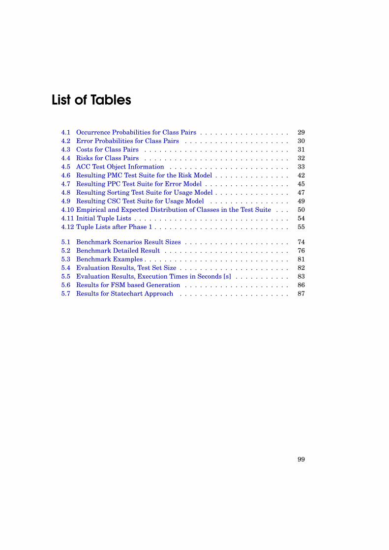
List of Tables
4.1 Occurrence Probabilities for Class Pairs . . . . . . . . . . . . . . . . . . 294.2 Error Probabilities for Class Pairs . . . . . . . . . . . . . . . . . . . . . 304.3 Costs for Class Pairs . . . . . . . . . . . . . . . . . . . . . . . . . . . . . 314.4 Risks for Class Pairs . . . . . . . . . . . . . . . . . . . . . . . . . . . . . 324.5 ACC Test Object Information . . . . . . . . . . . . . . . . . . . . . . . . 334.6 Resulting PMC Test Suite for the Risk Model . . . . . . . . . . . . . . . 424.7 Resulting PPC Test Suite for Error Model . . . . . . . . . . . . . . . . . 454.8 Resulting Sorting Test Suite for Usage Model . . . . . . . . . . . . . . . 474.9 Resulting CSC Test Suite for Usage Model . . . . . . . . . . . . . . . . 494.10 Empirical and Expected Distribution of Classes in the Test Suite . . . 504.11 Initial Tuple Lists . . . . . . . . . . . . . . . . . . . . . . . . . . . . . . . 544.12 Tuple Lists after Phase 1 . . . . . . . . . . . . . . . . . . . . . . . . . . . 55
5.1 Benchmark Scenarios Result Sizes . . . . . . . . . . . . . . . . . . . . . 745.2 Benchmark Detailed Result . . . . . . . . . . . . . . . . . . . . . . . . . 765.3 Benchmark Examples . . . . . . . . . . . . . . . . . . . . . . . . . . . . . 815.4 Evaluation Results, Test Set Size . . . . . . . . . . . . . . . . . . . . . . 825.5 Evaluation Results, Execution Times in Seconds [s] . . . . . . . . . . . 835.6 Results for FSM based Generation . . . . . . . . . . . . . . . . . . . . . 865.7 Results for Statechart Approach . . . . . . . . . . . . . . . . . . . . . . 87
99


Bibliography
[Aml00] Ståle Amland. Risk-based testing: Risk analysis fundamentals and met-rics for software testing including a financial application case study. Jour-nal of Systems and Software, 53(3):287–295, 2000.
[BC06] Renée C. Bryce and Charles J. Colbourn. Prioritized interaction testingfor pair-wise coverage with seeding and constraints. Information & Soft-ware Technology, 48(10):960–970, 2006.
[BC07] Renée C. Bryce and Charles J. Colbourn. The density algorithm for pair-wise interaction testing: Research articles. Softw. Test. Verif. Reliab.,17(3):159–182, 2007.
[BCM01] Simon Burton, John Clark, and John McDermid. Automated genera-tion of tests from statechart specifications. In Proceedings of Formal Ap-proaches to Testing Software (FATES) 2001, pages 31–46, August 2001.
[BE10] Dragan Bošnacki and Stefan Edelkamp. Model checking software: onsome new waves and some evergreens. Int. J. Softw. Tools Technol.Transf., 12:89–95, May 2010.
[Bin99] Robert V. Binder. Testing object-oriented systems: models, patterns, andtools. Addison-Wesley Longman Publishing Co., Inc., Boston, MA, USA,1999.
[BLLP04] Eddy Bernard, Bruno Legeard, Xavier Luck, and Fabien Peureux. Gener-ation of test sequences from formal specifications: GSM 11-11 standardcase study. Softw. Pract. Exper., 34:915–948, August 2004.
[Bry86] Randal E. Bryant. Graph-based algorithms for boolean function manipu-lation. IEEE Trans. Comput, 35:677–691, 1986.
[CC04] Charles J. Colbourn and Myra B. Cohen. A deterministic density algo-rithm for pairwise interaction coverage. In Proc. of the IASTED Intl.Conference on Software Engineering, pages 242–252, 2004.
[CDFP97] David M. Cohen, Siddhartha R. Dalal, Michael L. Fredman, and Gard-ner C. Patton. The AETG System: An Approach to Testing Based on Com-binatorial Design. IEEE Transactions on Software Engineering, 23:437–444, 1997.
101

Bibliography
[CDFY99] Mirko Conrad, Heiko Dörr, Ines Fey, and Andy Yap. Model-based Gen-eration and Structured Representation of Test Scenarios. In Proceedingsof the Workshop on Software-Embedded Systems Testing, Gaithersburg,Maryland, USA, 1999.
[CDS07] Myra B. Cohen, Matthew B. Dwyer, and Jiangfan Shi. Interaction testingof highly-configurable systems in the presence of constraints. In ISSTA’07: Proceedings of the 2007 international symposium on Software testingand analysis, pages 129–139, New York, NY, USA, 2007.
[CG10] Andrea Calvagna and Angelo Gargantini. A formal logic approach to con-strained combinatorial testing. Journal of Automated Reasoning, April2010.
[CGP99] Edmund M. Clarke, Orna Grumberg, and Doron A. Peled. Model Check-ing. MIT Press, 1999.
[Con05] Mirko Conrad. Systematic testing of embedded automotive software-theclassification-tree method for embedded systems (CTM/ES). Perspectivesof Model-Based Testing, 2005.
[CSR06] Myra B. Cohen, Joshua Snyder, and Gregg Rothermel. Testing acrossconfigurations: implications for combinatorial testing. SIGSOFT Softw.Eng. Notes, 31:1–9, November 2006.
[Cze06] Jacek Czerwonka. Pairwise testing in real world, practical extensions totest case generators. In Proceedings of 24th Pacific Northwest SoftwareQuality Conference, pages 419–430. Citeseer, 2006.
[EFW01] Ibrahim K. El-Far and James A. Whittaker. Model-Based Software Test-ing. Encyclopedia of Software Engineering, 2001.
[EMR02] Sebastian Elbaum, Alexey. G. Malishevsky, and Gregg Rothermel. Testcase prioritization: A family of empirical studies. IEEE Transactions onSoftware Engineering, 28(2):159–182, 2002.
[ERKM04] Sebastian Elbaum, Gregg Rothermel, Satya Kanduri, and Alexey G. Mal-ishevsky. Selecting a cost-effective test case prioritization technique.Software Quality Journal, 12:185–210, 2004.
[FKCA12] Javier Ferrer, Peter M. Kruse, J. Francisco Chicano, and Enrique Alba.Evolutionary algorithm for prioritized pairwise test data generation.In Proceedings of Genetic and Evolutionary Computation Conference(GECCO) 2012, Philadelphia, USA, 2012.
[GCD09] Brady J. Garvin, Myra B. Cohen, and Matthew B. Dwyer. An improvedmeta-heuristic search for constrained interaction testing. Search BasedSoftware Engineering, International Symposium on, 0:13–22, 2009.
102

Bibliography
[GFL+96] Daniel Geist, Monica Farkas, Avner Landver, Yossi Lichtenstein, ShmuelUr, and Yaron Wolfsthal. Coverage-directed test generation using sym-bolic techniques. In Proceedings of the First International Conference onFormal Methods in Computer-Aided Design, pages 143–158, London, UK,1996.
[GG93] Matthias Grochtmann and Klaus Grimm. Classification trees for parti-tion testing. Softw. Test., Verif. Reliab., 3(2):63–82, 1993.
[GOA05] Mats Grindal, Jeff Offutt, and Sten F. Andler. Combination testing strate-gies: a survey. Softw. Test., Verif. Reliab., 15(3):167–199, 2005.
[GPV+95] Rob Gerth, Doron Peled, Moshe Y. Vardi, R. Gerth, Den Dolech Eind-hoven, D. Peled, M. Y. Vardi, and Pierre Wolper. Simple on-the-fly au-tomatic verification of linear temporal logic. In In Protocol SpecificationTesting and Verification, pages 3–18. Chapman & Hall, 1995.
[GQW+09] Wolfgang Grieskamp, Xiao Qu, Xiangjun Wei, Nicolas Kicillof, andMyra B. Cohen. Interaction coverage meets path coverage by smt con-straint solving. In Proceedings of the 21st IFIP WG 6.1 International Con-ference on Testing of Software and Communication Systems and 9th In-ternational FATES Workshop, TESTCOM ’09/FATES ’09, pages 97–112,2009.
[GR01] Angelo Gargantini and Elvinia Riccobene. Asm-based testing: Coveragecriteria and automatic test sequence generation. Journal of UniversalComputer Science, 7:1050–1067, 2001.
[Har87] David Harel. Statecharts: a visual formalism for complex systems. Sci-ence of Computer Programming, 8(3):231–274, 1987.
[He09] Yuxiong He. Multicore-enabling a binary decision diagram algorithm,2009.
[Hel07] Steffen Helke. Verifikation von Statecharts durch struktur- und eigen-schaftserhaltende Datenabstraktion. PhD thesis, Technische UniversitätBerlin, 2007.
[HHS03] Robert M. Hierons, Mark Harman, and Harbhajan Singh. Automaticallygenerating information from a Z specification to support the Classifica-tion Tree Method. In 3rd International Conference of B and Z Users,LNCS volume 2651, pages 388–407, June 2003.
[HRSR09] Andreas Hoffmann, Axel Rennoch, Ina Schieferdecker, and Nicole Radzi-will. A generic approach for modeling test case priorities with appli-cations for test development and execution. In Modellbasiertes Testen(MOTES)–Von der Forschung in die Praxis (2009), 4. Workshop im Rah-men der 39. Jahrestagung der GI, 2009.
103

Bibliography
[HRV+03] Mats P.E. Heimdahl, S. Rayadurgam, Willem Visser, George Devaraj,and Jimin Gao. Auto-generating test sequences using model checkers:A case study. In Proceedings of Formal Approaches to Testing of Software(FATES 2003), 2003.
[Jan05] Ben Jann. Einführung in die Statistik. Oldenbourg, 2005.
[JM09] Ranjit Jhala and Rupak Majumdar. Software model checking. ACM Com-put. Surv., 41:21:1–21:54, October 2009.
[KKL10] D. Richard Kuhn, Raghu N. Kacker, and Yu Lei. Practical combinatorialtesting. Technical report, National Institute for Standards and Technol-ogy (NIST), October 2010.
[KL10a] Peter M. Kruse and Magdalena Luniak. Automated test case generationusing classification trees. In Proceedings of StarEast 2010, 2010.
[KL10b] Peter M. Kruse and Magdalena Luniak. Automated test case genera-tion using classification trees. Software Quality Professional, 13(1):4–12,2010.
[KL11] Peter. M. Kruse and Kiran Lakhotia. Multi objective algorithms for auto-mated generation of combinatorial test cases with the classification treemethod. In Symposium On Search Based Software Engineering (SSBSE2011), 2011.
[KLK08] Rick Kuhn, Yu Lei, and Raghu Kacker. Practical Combinatorial Testing:Beyond Pairwise. IT Professional, 10(3):19–23, 2008.
[KM05] Alexander Krupp and Wolfgang Müller. Modelchecking vonKlassifikationsbaum-Testsequenzen. In GI/ITG/GMM Workshop"Methoden und Beschreibungssprachen zur Modellierung und Verifika-tion von Schaltungen und Systemen", April 2005.
[Kru11] Peter M. Kruse. Test sequence generation from classification trees usingmulti-agent systems. In Proceedings of 9th European Workshop on Multi-agent Systems (EUMAS 2011), 2011.
[KS12] Peter M. Kruse and Ina Schieferdecker. Comparison of Approaches to Pri-oritized Test Generation for Combinatorial Interaction Testing. In Fed-erated Conference on Computer Science and Information Systems (FedC-SIS) 2012, Wroclaw, Poland, 2012.
[KW11a] Peter M. Kruse and Joachim Wegener. Sequenzgenerierung aus Klassi-fikationsbäumen. In Proceedings zum 31. Treffen der Fachgruppe TAVder Gesellschaft für Informatik, Paderborn, Germany, 2011.
104

Bibliography
[KW11b] Peter M. Kruse and Joachim Wegener. Test sequence generation fromclassification trees. In Sistemas e Tecnologias de Informação, Actas da6a Conferência Ibérica de Sistemas e Tecnologias de Informação, Chaves,Portugal, 2011.
[KW12] Peter M. Kruse and Joachim Wegener. Test sequence generation fromclassification trees. In Proceedings of ICST 2012 Workshops (ICSTW2012), Montreal, Canada, 2012.
[Lee59] C.Y. Lee. Representation of switching circuits by binary-decision pro-grams. Bell System Technical Journal, 38(4):985–999, 1959.
[LT98] Yu Lei and Kuo-Chung Tai. In-parameter-order: A test generation strat-egy for pairwise testing. In The 3rd IEEE International Symposium onHigh-Assurance Systems Engineering, HASE ’98, pages 254–261, Wash-ington, DC, USA, 1998.
[Luc93] Paul J. Lucas. An Object-Oriented Language System For ImplementingConcurrent, Hierarchical, Finite State Machines. PhD thesis, GraduateCollege of the University of Illinois at Urbana-Champaign, 1993.
[Lun09] Magdalena Luniak. Priorisierende Kombinationsregeln in derKlassifikationsbaum-Methode. Master’s thesis, Technische UniversitätBerlin, 2009.
[LW00] Eckard Lehmann and Joachim Wegener. Test case design by means ofthe CTE XL. In Proceedings of the 8th European International Conferenceon Software Testing, Analysis & Review (EuroSTAR 2000), Kopenhagen,Denmark. Citeseer, 2000.
[Mir09] Mirosamek. Two orthogonal regions (main key-pad and numeric keypad) of a computer keyboard.http://en.wikipedia.org/wiki/File:UML_state_machine_Fig4.png, 2009.
[MN05] Soumen Maity and Amiya Nayak. Improved test generation algorithmsfor pair-wise testing. In ISSRE, pages 235–244. IEEE Computer Society,2005.
[MTR08] Alessandro Marchetto, Paolo Tonella, and Filippo Ricca. State-based test-ing of Ajax web applications. In In Proceedings of the International Con-ference on Software Testing (ICST 2008), April 2008.
[Mye79] Glenford J. Myers. The Art of Software Testing. John Wiley & Sons, 1979.
[NL11] Changhai Nie and Hareton Leung. A survey of combinatorial testing.ACM Comput. Surv., 43:11:1–11:29, February 2011.
105
Bibliography
[OB88] Thomas J. Ostrand and Marc J. Balcer. The category-partition method forspecifying and generating functional tests. Communications of the ACM,31(6):676–686, 1988.
[Obj10] Object Management Group. OMG Unified Modeling Language (OMGUML), Superstructure Verion 2.3, 2010.
[OHY11] Jungsup Oh, Mark Harman, and Shin Yoo. Transition coverage test-ing for Simulink/Stateflow models using messy genetic algorithms. InGenetic Algorithms and Evolutionary Computation COnference (GECCO2011), pages 1851–1858, July 2011.
[Pun04] Abraham P. Punnen. The traveling salesman problem: Applications,formulations and variations. In The Traveling Salesman Problem andIts Variations, volume 12 of Combinatorial Optimization, pages 1–28.Springer, 2004.
[Rei10] Robert Reicherdt. Testfallgenerierung mit Binary Decision Diagrams fürKlassifikationsbäume mit Abhängigkeiten. Master’s thesis, TechnischeUniversität Berlin, 2010.
[Sch13] Henno Schooljahn. Test Sequence Validation and Generation using Clas-sification Trees. Master’s thesis, Delft University of Technology, 2013.
[Sed03] Robert Sedgewick. Algorithms in Java - Part 5: Graph Algorithms.Addison-Wesley, Boston, MA, USA, 3 edition, 2003.
[SRG11] Elke Salecker, Robert Reicherdt, and Sabine Glesner. Calculating pri-oritized interaction test sets with constraints using binary decision dia-grams. In Proceedings of the 2011 IEEE Fourth International Conferenceon Software Testing, Verification and Validation Workshops, ICSTW ’11,pages 278–285, Washington, DC, USA, 2011. IEEE Computer Society.
[Ura92] Hasan Ural. Formal methods for test sequence generation. Comput. Com-mun., 15:311–325, June 1992.
[Var01] Moshe Y. Vardi. Branching vs. linear time: Final showdown. In Proceed-ings of the 7th International Conference on Tools and Algorithms for theConstruction and Analysis of Systems, TACAS 2001, pages 1–22, London,UK, 2001.
[Wal11] Nick Walther. Testsequenz-Generierung und Repräsentation mit derKlassifikationsbaum-Methode. Master’s thesis, Humbold UniversitätBerlin, 2011.
[WG93] Joachim Wegener and Matthias Grochtmann. Werkzeugunter-stützte Testfallermittlung für den funktionalen Test mit demKlassifikationsbaum-Editor CTE. In Proceedings of the GI-SymposiumSoftwaretechnik ’93, pages 95–102, Dortmund, 1993.
106

Bibliography
[Wil02] Alan W. Williams. Software Component Interaction Testing: CoverageMeasurement and Generation of Configurations. PhD thesis, School ofInformation Technology and Engineering, University of Ottawa, 2002.
[Win08] Andreas Windisch. Search-based testing of complex simulink models con-taining stateflow diagrams. In Proceedings of 1st International Workshopon Search-Based Software Testing (SBST) in conjunction with ICST 2008,pages 251–251, Lillehammer, Norway, 9-11 April 2008.
[Win10] Andreas Windisch. Search-based test data generation from stateflowstatecharts. In Proceedings of the 12th annual conference on Genetic andevolutionary computation, GECCO ’10, pages 1349–1356, New York, NY,USA, 2010.
[WLPS00] Guido Wimmel, Heiko Loetzbeyer, Alexander Pretschner, and Oscar Slo-tosch. Specification based test sequence generation with propositionallogic, 2000.
[WP01] Alan W. Williams and Robert L. Probert. A measure for component inter-action test coverage. In Proc. ACS/IEEE Intl. Conf. on Computer Systemsand Applications, volume 30, pages 301–311, 2001.
[WPT95] Gwendolyn H. Walton, Jesse H. Poore, and Carmen J. Trammell. Sta-tistical testing of software based on a usage model. Softw. Pract. Exper.,25(1):97–108, 1995.
[YH10] Shin Yoo and Mark Harman. Using hybrid algorithm for pareto effcientmulti-objective test suite minimisation. Journal of Systems Software,83(4):689–701, April 2010.
107


A Appendix
A.1 Test Sequence Generation Examples
In this section, we provide all examples for the test sequence generation benchmarks.Each example consists of a classification tree with added ID values for all tree
elements to avoid any ambiguity. In square brackets with a leading S : we providea list of corresponding start nodes for each classification. The list of all transitionsfrom within this classification concerning all contained classes is provided as commaseparated list.
Each transition (a → b) represents a directed transition from a to b. ID values forall classes are provided for clarity.
Multiple transitions from a to b are provided as often as they occur leading torepetition in the list.
Transitions from a in one classification A to any b in a different classification B areonly listed in the classification of origin A.
keyboard.cte
Example Keyboard States [Mir09]: A typical PC desktop keyboard features at leasttwo regions: The main area with all characters and a number pad. Both regionshave their own modes. While the main area has the caps lock feature, to input onlyuppercase letters, the number pad can be switched between numbers and arrowsusing the num lock button. Both regions and their states are independent of eachother. In the classification tree keyboard (Figure A.1), there is one classification perkeyboard region. Each classification has two classes representing the correspondingstates.
Figure A.1: Keyboard Example
109

A Appendix
main_keyboard(18) [S : default(26)] :
(default(26)→ default(26)), (default(26)→ caps_lock(30)),
(caps_lock(30)→ caps_lock(30)), (caps_lock(30)→ default(26))
numeric_keyboard(22) [S : numbers(34)] :
(numbers(34)→ numbers(34)), (numbers(34)→ arrows(38)),
(arrows(38)→ arrows(38)), (arrows(38)→ numbers(34))
microwave.cte
Microwave Example [Luc93]: The example microwave device has three independentfunction blocks. It features a Light, Display and a Mode. All three features areindependent of each other. The Light can be on and off while the Display eithershows Time or Not-Time. If it shows Not-Time, then it shows one of Counter, Poweror Error. The Mode can be Operational or Disabled. If Mode is Operational, then itis one of Idle, Set-Time, Program, or Cook.
Figure A.2: Microwave Example
Mode(17) [S : Operational(57)] :
(Operational(57)→ Disabled(61)), (Disabled(61)→ Operational(57))
Display(20) [S : Time(34)] :
(Time(34)→ Counter(45)), (Not – Time(38)→ Time(34)),
(Time(34)→ Error(53))
Light(23) [S : Off (26)] :
(Off (26)→ On(30)), (On(30)→ Off (26))
110

A.1 Test Sequence Generation Examples
Operational(65) [S : Idle(68)] :
(Idle(68)→ Set – Time(72)), (Set – Time(72)→ Idle(68)),
(Idle(68)→ Program(76)), (Program(76)→ Idle(68)),
(Program(76)→ Cook(80)), (Cook(80)→ Program(76)),
(Idle(68)→ Cook(80)), (Cook(80)→ Idle(68))
Not – Time(42) [S : ()] : (Counter(45)→ Power(49)), (Power(49)→ Counter(45))
Set – Time(108) [S : Setting(111)] :
(Setting(111)→ Error(115)), (Setting(111)→ Setting(111))
Program(119) [S : Setting(122)] :
(Setting(122)→ Power(126)), (Power(126)→ Setting(122)),
(Setting(122)→ Setting(122))
Cook(130) [S : RealCook(133)] :
(RealCook(133)→ RealCook(133))
autoradio.cte
Car Radio Example [Hel07]: The car radio consists of three main classifications, aCD Drive (CD Fach), a Tape Deck (Cassetten Fach) and a Control Unit (Steuerung).The CD Drive has three modes, which are Empty (cd_leer), Reading (Titel einlesen)and Loaded (cd_voll). The Tape Deck only has Empty (t_leer) and Loaded (t_voll).The Control Unit can either be On (An) or Off (Aus). If it is on, then there are threedistinct playback options: Radio Modus, Cassette Modus and CD Modus. Each optionfeatures its own charateristics, there are 4 radio station keys, for example.
Figure A.3: Autoradio Example
111
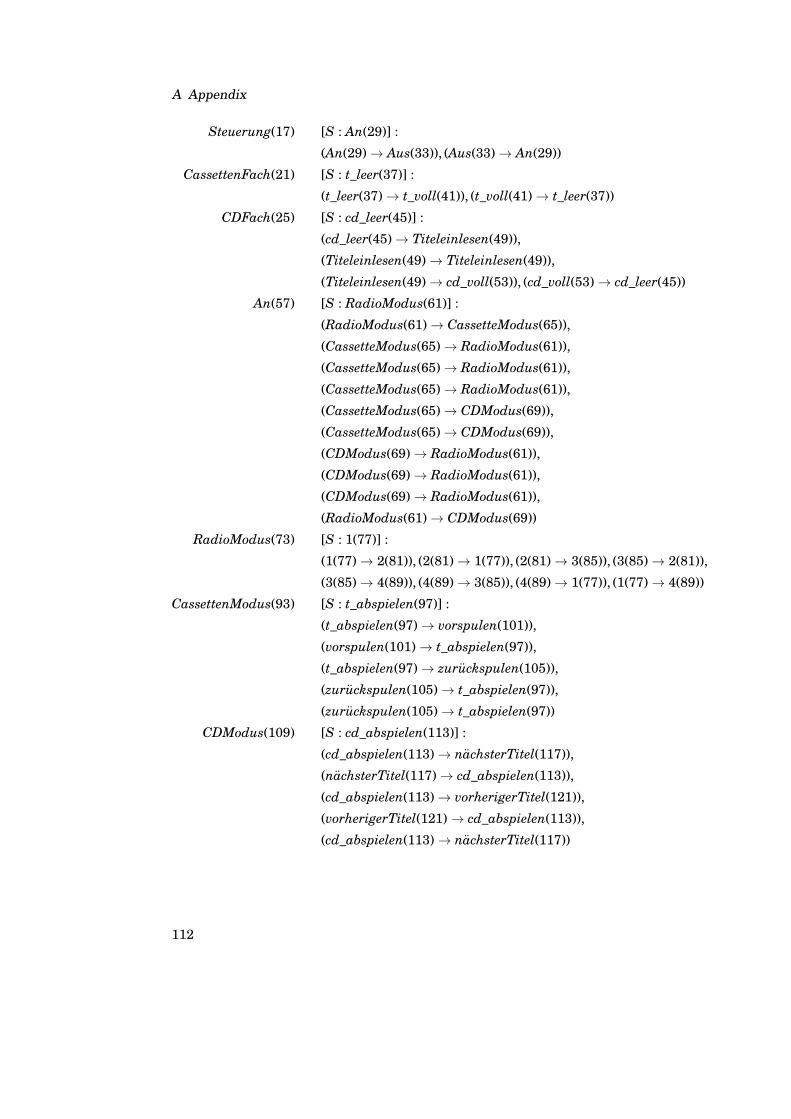
A Appendix
Steuerung(17) [S : An(29)] :
(An(29)→ Aus(33)), (Aus(33)→ An(29))
CassettenFach(21) [S : t_leer(37)] :
(t_leer(37)→ t_voll(41)), (t_voll(41)→ t_leer(37))
CDFach(25) [S : cd_leer(45)] :
(cd_leer(45)→ Titeleinlesen(49)),
(Titeleinlesen(49)→ Titeleinlesen(49)),
(Titeleinlesen(49)→ cd_voll(53)), (cd_voll(53)→ cd_leer(45))
An(57) [S : RadioModus(61)] :
(RadioModus(61)→ CassetteModus(65)),
(CassetteModus(65)→ RadioModus(61)),
(CassetteModus(65)→ RadioModus(61)),
(CassetteModus(65)→ RadioModus(61)),
(CassetteModus(65)→ CDModus(69)),
(CassetteModus(65)→ CDModus(69)),
(CDModus(69)→ RadioModus(61)),
(CDModus(69)→ RadioModus(61)),
(CDModus(69)→ RadioModus(61)),
(RadioModus(61)→ CDModus(69))
RadioModus(73) [S : 1(77)] :
(1(77)→ 2(81)), (2(81)→ 1(77)), (2(81)→ 3(85)), (3(85)→ 2(81)),
(3(85)→ 4(89)), (4(89)→ 3(85)), (4(89)→ 1(77)), (1(77)→ 4(89))
CassettenModus(93) [S : t_abspielen(97)] :
(t_abspielen(97)→ vorspulen(101)),
(vorspulen(101)→ t_abspielen(97)),
(t_abspielen(97)→ zuruckspulen(105)),
(zuruckspulen(105)→ t_abspielen(97)),
(zuruckspulen(105)→ t_abspielen(97))
CDModus(109) [S : cd_abspielen(113)] :
(cd_abspielen(113)→ nachsterTitel(117)),
(nachsterTitel(117)→ cd_abspielen(113)),
(cd_abspielen(113)→ vorherigerTitel(121)),
(vorherigerTitel(121)→ cd_abspielen(113)),
(cd_abspielen(113)→ nachsterTitel(117))
112

A.1 Test Sequence Generation Examples
citizen.cte
Citizen Watch [Har87]: The Citizen Watch was Harel’s original example to introduceStatecharts in [Har87].
The watch can either be alive or dead. If it is alive, then it consists of six parellelactivities, which are main, alarm1-status, alarm2-status, chime-status, light, andpower. While the other five activities can be only disabled or enabled, basically, Mainis divided into severeal further substates. They are display and alarm-beep. If thewatch is on alarm-beep, then it is alarm 1 beep, alarm 2 beep or both beep.. If thewatch is not on alarm beep, it is on display. The display can be one of regular, wait,out or stopwatch, which are then further refined.
We skip the rest of description and refer to the figures for further details.
Figure A.4: Citizen Example
Figure A.5: Citizen Example
113

A Appendix
Figure A.6: Citizen Example
Citizen(17) [S : dead(25)] :
(dead(25)→ alive(21)), (alive(21)→ dead(25))
main(281) [S : display(285)] :
(display(285)→ alarm1beep(297)), (display(285)→ alarm2beep(301)),
(display(285)→ bothbeep(305)), (alarm – beep(289)→ display(285))
alarm1 – status(33) [S : disabled(309)] :
(disabled(309)→ enabled(313)), (enabled(313)→ disabled(309))
alarm2 – status(49) [S : disabled(317)] :
(disabled(317)→ enabled(321)), (enabled(321)→ disabled(317))
enabled(349) [S : ()] :
(quiet(353)→ beep(357)), (beep(357)→ quiet(353))
chime – status(37) [S : disabled(325)] :
(disabled(325)→ quiet(353)), (enabled(329)→ disabled(325))
light(41) [S : off (337)] :
(off (337)→ on(333)), (on(333)→ off (337))
power(45) [S : ok(341)] :
(ok(341)→ blink(345)), (blink(345)→ dead(25))
display(29) [S : regular(69)] :
(out(65)→ regular(69)), (stopwatch(61)→ regular(69)),
(wait(57)→ sec(117))
114
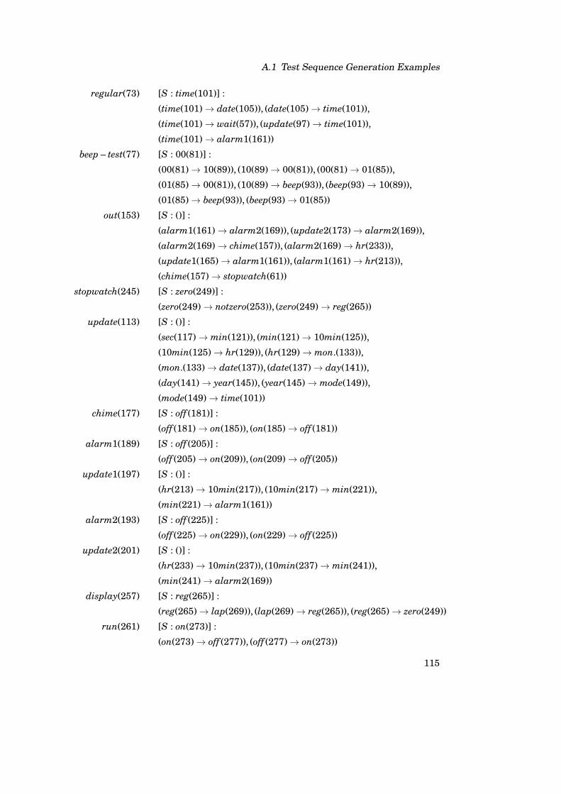
A.1 Test Sequence Generation Examples
regular(73) [S : time(101)] :
(time(101)→ date(105)), (date(105)→ time(101)),
(time(101)→ wait(57)), (update(97)→ time(101)),
(time(101)→ alarm1(161))
beep – test(77) [S : 00(81)] :
(00(81)→ 10(89)), (10(89)→ 00(81)), (00(81)→ 01(85)),
(01(85)→ 00(81)), (10(89)→ beep(93)), (beep(93)→ 10(89)),
(01(85)→ beep(93)), (beep(93)→ 01(85))
out(153) [S : ()] :
(alarm1(161)→ alarm2(169)), (update2(173)→ alarm2(169)),
(alarm2(169)→ chime(157)), (alarm2(169)→ hr(233)),
(update1(165)→ alarm1(161)), (alarm1(161)→ hr(213)),
(chime(157)→ stopwatch(61))
stopwatch(245) [S : zero(249)] :
(zero(249)→ notzero(253)), (zero(249)→ reg(265))
update(113) [S : ()] :
(sec(117)→ min(121)), (min(121)→ 10min(125)),
(10min(125)→ hr(129)), (hr(129)→ mon.(133)),
(mon.(133)→ date(137)), (date(137)→ day(141)),
(day(141)→ year(145)), (year(145)→ mode(149)),
(mode(149)→ time(101))
chime(177) [S : off (181)] :
(off (181)→ on(185)), (on(185)→ off (181))
alarm1(189) [S : off (205)] :
(off (205)→ on(209)), (on(209)→ off (205))
update1(197) [S : ()] :
(hr(213)→ 10min(217)), (10min(217)→ min(221)),
(min(221)→ alarm1(161))
alarm2(193) [S : off (225)] :
(off (225)→ on(229)), (on(229)→ off (225))
update2(201) [S : ()] :
(hr(233)→ 10min(237)), (10min(237)→ min(241)),
(min(241)→ alarm2(169))
display(257) [S : reg(265)] :
(reg(265)→ lap(269)), (lap(269)→ reg(265)), (reg(265)→ zero(249))
run(261) [S : on(273)] :
(on(273)→ off (277)), (off (277)→ on(273))
115

A Appendix
coffee.cte
Coffee Machine Example: IBM Rhapsody features this example of a commercial cof-fee machine. It consists of the actual CoffeeMachine, a Display and a Boiler. All threeof them can be either off or on independent of each other.
If the CoffeeMachine is on, its Main state is either idle or working while the Powerstate is always in its working mode. If the machine is idle, it can be in waitMain-tenance or in readyForCoin. When a coin is supplied, the machine changes to itsworking state and produces a cup of coffee step by step: fillCoffee, pressurize, fillWa-ter, fillMilk, fillCup, and cupReady.
The display shows progress messages either permanent or rotating.The boiler has a temperatur sensor and cam boilWater or keepTemp.
Figure A.7: Coffee Machine Example
CoffeeMachine(19) [S : off (23)] :
(off (23)→ on(27)), (on(27)→ off (23))
Display(137) [S : off (145)] :
(off (145)→ on(149)), (on(149)→ off (145)),
(off (145)→ off (145))
Boiler(215) [S : off (219)] :
(off (219)→ off (219)), (off (219)→ on(223)),
(on(223)→ off (219))
Main(31) [S : idle(39)] :
Power(35) [S : powerControl(87)] :
116

A.1 Test Sequence Generation Examples
Message(153) [S : permanent(157)] :
(permanent(157)→ rotating(161)),
(rotating(161)→ permanent(157)),
(rotating(161)→ rotating(161))
On(227) [S : boilWater(231)] :
(boilWater(231)→ keepTemp(235)),
(keepTemp(235)→ boilWater(231))
Idle(47) [S : waitMaintenance(51)] :
(waitMaintenance(51)→ readyForCoin(55)),
(readyForCoin(55)→ waitMaintenance(51)),
(readyForCoin(55)→ working(43))
Working(59) [S : fillCoffee(63)] :
(fillCoffee(63)→ fillCoffee(63)),
(fillCoffee(63)→ pressurize(67)),
(pressurize(67)→ pressurize(67)),
(pressurize(67)→ fillWater(71)),
(fillWater(71)→ fillWater(71)),
(fillWater(71)→ fillMilk(75)),
(fillMilk(75)→ fillMilk(75)),
(fillMilk(75)→ fillCup(79)),
(fillCup(79)→ fillCup(79)),
(fillCup(79)→ cupReady(83)),
(cupReady(83)→ idle(39))
communication.cte
Communication Example: IBM Rhapsody features this example of a communica-tion software. The State of the software can either be Disabled or Enabled. If it isEnabled, it can be Idle, Receiving or Transmitting. In Receiving, the software is Wait-ing_for_Byte, Validating_Command or Processing. In Transmitting, the software isWaiting_for_Timeout or Waiting_for_Transmit_Timeout.
117

A Appendix
Figure A.8: Communication Example
State(20) [S : Disabled(24)] :
(Disabled(24)→ Idle(36)), (Enabled(28)→ Disabled(24))
Enabled(32) [S : Idle(36)] :
(Idle(36)→ Recieving(40)), (Idle(36)→ Transmitting(44))
Recieving(48) [S : Waiting_For_Byte(52)] :
(Waiting_For_Byte(52)→Waiting_For_Byte(52)),
(Waiting_For_Byte(52)→ Validating_Command(56)),
(Validating_Command(56)→ Processing(60)),
(Validating_Command(56)→ Transmitting(44)),
(Processing(60)→ Transmitting(44))
Transmitting(64) [S : Waiting_For_Timeout(68)] :
(Waiting_For_Timeout(68)→Waiting_For_Timeout(68)),
(Waiting_For_Timeout(68)→Waiting_For_Transmit_Timeout(72)),
(Waiting_For_Transmit_Timeout(72)→ Idle(36))
elevator.cte
Elevator Example: IBM Rhapsody features this example of an elevator. The elevatoroperation is defined by an Action, Direction, Door and Building. Actions can be wait,changeDirection, moving, openingDoor and closingDoor. Directions are goingUp andgoingDown. The door is either closed, opening, open, or closing. The building is eithernormal or simulated.
118

A.1 Test Sequence Generation Examples
Figure A.9: Elevator Example
Action(26) [S : wait(42)] :
(wait(42)→ changeDirection(46)),
(changeDirection(46)→ wait(42)),
(wait(42)→ moving(50)),
(wait(42)→ openingDoor(54)),
(moving(50)→ openingDoor(54)),
(openingDoor(54)→ closingDoor(58)),
(closingDoor(58)→ wait(42)), (moving(50)→ moving(50))
Direction(30) [S : goingUp(34)] :
(goingUp(34)→ goingDown(38)), (goingDown(38)→ goingUp(34))
Door(120) [S : closed(124)] :
(closed(124)→ opening(128)), (opening(128)→ open(132)),
(open(132)→ closing(136)), (closing(136)→ closed(124))
Building(140) [S : normal(144)] :
(normal(144)→ normal(144)), (normal(144)→ simulated(148)),
(simulated(148)→ simulated(148)),
(simulated(148)→ normal(144))
tetris.cte
Tetris Example: IBM Rhapsody features this example of a Tetris game. The gamecan either be ready, startingGame, newPiece, runningGame, paused, removePlace, orgameOver. RunningGame is further refined into startUp, controlling, dropping, anddropped. There are no parallel activities involved in this example.
119

A Appendix
Figure A.10: Tetris Example
Game(19) [S : ready(23)] :
(ready(23)→ startingGame(27)),
(startingGame(27)→ newPiece(31)),
(newPiece(31)→ runningGame(35)),
(runningGame(35)→ paused(39)),
(paused(39)→ runningGame(35)),
(removePiece(43)→ newPiece(31)),
(removePiece(43)→ newPiece(31)),
(paused(39)→ gameOver(47)),
(gameOver(47)→ startingGame(27)),
(runningGame(35)→ gameOver(47))
runningGame(85) [S : startup(89)] :
(startup(89)→ controlling(93)),
(controlling(93)→ dropping(97)),
(controlling(93)→ dropped(101)),
(dropping(97)→ dropped(101)),
(startup(89)→ gameOver(47)),
(dropping(97)→ dropping(97)),
(controlling(93)→ controlling(93)),
(dropped(101)→ controlling(93)),
(dropped(101)→ removePiece(43))
120

A.1 Test Sequence Generation Examples
moore.cte
Moore Example: Matlab Simulink Stateflow features this example. States are s0, s1,s12, s121, s1123. There are no parallel activities involved in this example.
Figure A.11: Moore Example
seqrec(19) [S : s0(23)] :
(s0(23)→ s1(27)), (s1(27)→ s0(23)), (s1(27)→ s12(31)),
(s12(31)→ s0(23)), (s12(31)→ s121(35)), (s121(35)→ s12(31)),
(s121(35)→ s0(23)), (s121(35)→ s1(27)), (s121(35)→ s1213(39)),
(s1213(39)→ s0(23)), (s1213(39)→ s1(27))
fuel.cte
Fuel Example: Matlab Simulink Stateflow features this example. Parellel statesconsist of O2, Pressure, Throttle, Speed, Fail and Fueling_Mode. Oxygen O2 can beO2_warmup, O2_normaln and O2_failure. All three Pressure, Throttle and Speedcan be normal and fail. The Fail state indicates the number of fails, it can beNone, One and Multi. Multi is then further refined into Two, Three and Four. TheFueling Mode is one of Running and Fuel_Disabled. If it is Running, it is oneof Low_Emissions (with Warmup and Normal) and Rich_Mixture (with only Sin-gle_Failure). Fuel_Disabled can be due to Overspeed or Shutdown.
121

A Appendix
Figure A.12: Fuel Example
O2(19) [S : A(147)] :
Pressure(23) [S : normal(139)] :
(normal(139)→ fail(143)), (fail(143)→ normal(139))
Throttle(27) [S : normal(131)] :
(normal(131)→ fail(135)), (fail(135)→ normal(131))
Speed(31) [S : normal(123)] :
(normal(123)→ fail(127)), (fail(127)→ normal(123))
Fail(35) [S : None(43)] :
(None(43)→ One(47)), (One(47)→ None(43)),
(One(47)→ Two(59))
Fueling_Mode(39) [S : Running(71)] :
(Running(71)→ Overspeed(115)),
(Running(71)→ Shutdown(119))
A(151) [S : O2_warmup(155)] :
(O2_warmup(155)→ O2_normal(159)),
(O2_normal(159)→ O2_failure(163)),
(O2_failure(163)→ O2_normal(159))
Multi(55) [S : ()] :
(Two(59)→ Three(63)), (Three(63)→ Two(59)),
(Three(63)→ Four(67)), (Four(67)→ Three(63)),
(Two(59)→ One(47))
Running(79) [S : Low_Emissions(83)] :
122
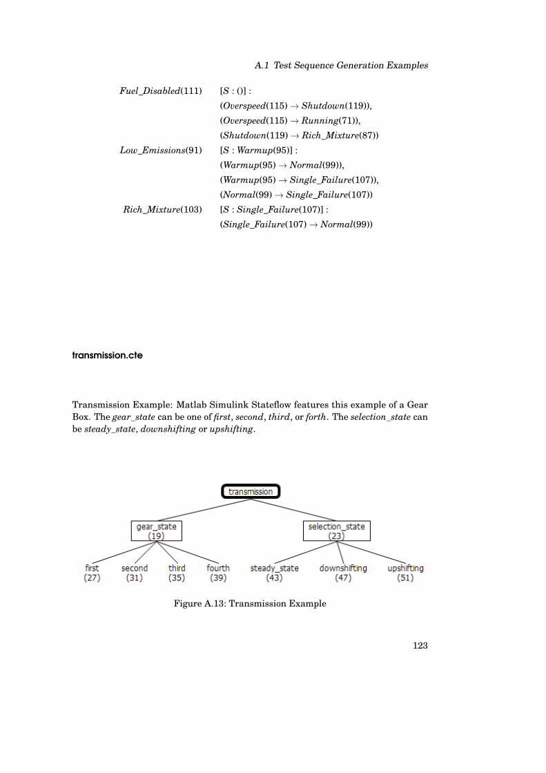
A.1 Test Sequence Generation Examples
Fuel_Disabled(111) [S : ()] :
(Overspeed(115)→ Shutdown(119)),
(Overspeed(115)→ Running(71)),
(Shutdown(119)→ Rich_Mixture(87))
Low_Emissions(91) [S : Warmup(95)] :
(Warmup(95)→ Normal(99)),
(Warmup(95)→ Single_Failure(107)),
(Normal(99)→ Single_Failure(107))
Rich_Mixture(103) [S : Single_Failure(107)] :
(Single_Failure(107)→ Normal(99))
transmission.cte
Transmission Example: Matlab Simulink Stateflow features this example of a GearBox. The gear_state can be one of first, second, third, or forth. The selection_state canbe steady_state, downshifting or upshifting.
Figure A.13: Transmission Example
123

A Appendix
gear_state(19) [S : first(27)] :
(first(27)→ second(31)), (second(31)→ third(35)),
(third(35)→ fourth(39)), (fourth(39)→ third(35)),
(third(35)→ second(31)), (second(31)→ first(27))
selection_state(23) [S : steady_state(43)] :
(steady_state(43)→ downshifting(47)),
(downshifting(47)→ steady_state(43)),
(downshifting(47)→ steady_state(43)),
(steady_state(43)→ upshifting(51)),
(upshifting(51)→ steady_state(43)),
(upshifting(51)→ steady_state(43))
aircraft.cte
Aircraft Example: Matlab Simulink Stateflow features this example of a redundantaircraft sub system. One component exists four times: LO, RO, LI, and RI. Each itemcan be L1 or isolated. If it is L1, then it is one of passive, standby, active, or off.
Figure A.14: Aircraft Example
124

A.1 Test Sequence Generation Examples
LO(19) [S : L1(39)] :
(L1(39)→ isolated(35))
RO(2335) [S : L1(2355)] :
(L1(2355)→ isolated(2347))
LI(2303) [S : L1(2323)] :
(L1(2323)→ isolated(2315))
RI(2271) [S : L1(2291)] :
(L1(2291)→ isolated(2283))
normal(43) [S : passive(47)] :
(passive(47)→ active(51)), (passive(47)→ standby(55)),
(active(51)→ standby(55), (standby(55)→ active(51))
normal(2327) [S : passive(2351)] :
(passive(2351)→ standby(2339)), (passive(2351)→ active(2343)),
(standby(2339)→ active(2343)), (active(2343)→ standby(2339))
normal(2295) [S : passive(2319)] :
(passive(2319)→ standby(2307)), (passive(2319)→ active(2311)),
(standby(2307)→ active(2311)), (active(2311)→ standby(2307))
normal(2263) [S : passive(2287)] :
(passive(2287)→ standby(2275)), (standby(2275)→ active(2279)),
(passive(2287)→ active(2279)), (active(2279)→ standby(2275))
125


Versicherung
Ich erkläre, dass ich die vorliegende Dissertation selbständig und eigenhändig ange-fertigt und keine anderen als die von mir angegebenen Quellen und Hilfsmittel ver-wendet habe.
Ich erkläre weiterhin, dass die Dissertation bisher nicht in dieser oder andererForm in einem anderen Prüfungsverfahren vorgelegen hat.
——————————————Berlin, den