Engineering the quantitative PCR assay fordecreased cost and complexity

by

Gregory J. Boggy

A dissertation submitted in partial fulfillmentof the requirements for the degree of

Doctor of Philosophy(Chemical Engineering)

in The University of Michigan2011

Doctoral Committee:

Assistant Professor Peter J. Woolf, Co-ChairAssistant Professor Xiaoxia Lin, Co-ChairProfessor Jennifer J. LindermanAssistant Professor David K. Lubensky

c© Gregory J. Boggy 2011

All Rights Reserved

For Karen and Jasmine.

ii

ACKNOWLEDGEMENTS

I owe a tremendous debt of gratitude to my advisor, Peter Woolf, who gave me

the freedom to explore many paths to find the one that led me toward my goals.

Through Peter’s mentoring, I have developed as a researcher, an innovator, a teacher,

and a leader. It has been an honor and a pleasure working under his guidance.

I owe thanks to colleagues at DNA Software, Inc. of Ann Arbor, where I worked

briefly during graduate school. I have learned a great deal about nucleic acids, the

polymerase chain reaction, and biotechnology in general, during my time at DNA

Software. DNA Software’s products have also proved invaluable for the design of my

experiments.

I owe many thanks to my family, whose emotional support helped weather the

disappointments inevitably encountered in research. I especially owe thanks to my

wife Karen and my father, who both went above and beyond the call of duty to

support me in my work.

Finally, I owe thanks to my colleagues in graduate school who helped make grad-

uate school an enjoyable experience. I will value the friendships I have developed

during graduate school for the rest of my life.

iii

TABLE OF CONTENTS

DEDICATION . . . . . . . . . . . . . . . . . . . . . . . . . . . . . . . . . . ii

ACKNOWLEDGEMENTS . . . . . . . . . . . . . . . . . . . . . . . . . . iii

LIST OF FIGURES . . . . . . . . . . . . . . . . . . . . . . . . . . . . . . . vii

LIST OF TABLES . . . . . . . . . . . . . . . . . . . . . . . . . . . . . . . . ix

LIST OF APPENDICES . . . . . . . . . . . . . . . . . . . . . . . . . . . . x

LIST OF ABBREVIATIONS . . . . . . . . . . . . . . . . . . . . . . . . . xi

ABSTRACT . . . . . . . . . . . . . . . . . . . . . . . . . . . . . . . . . . . xii

CHAPTER

I. Introduction . . . . . . . . . . . . . . . . . . . . . . . . . . . . . . 1

1.1 Decreasing the cost of accurate qPCR quantification . . . . . 21.1.1 Hypothesis: Biophysics-based qPCR quantification

enables high accuracy quantification at low cost . . 41.2 Decreasing cost and complexity of multiplex qPCR . . . . . . 5

1.2.1 Quantitative PCR detection chemistries . . . . . . . 61.2.2 Cost of specific qPCR detection . . . . . . . . . . . 71.2.3 Complexity of specific qPCR detection . . . . . . . 81.2.4 Quantitative limitations of multiplex qPCR . . . . . 81.2.5 Hypothesis: Monochrome multiplex qPCR and mech-

anistic quantification enables simple and accurate mul-tiplex measurement of DNA targets at low cost . . . 9

1.3 Thesis Overview . . . . . . . . . . . . . . . . . . . . . . . . . 10

II. Biophysics of PCR . . . . . . . . . . . . . . . . . . . . . . . . . . 12

2.1 Introduction . . . . . . . . . . . . . . . . . . . . . . . . . . . 122.2 Overview of the polymerase chain reaction . . . . . . . . . . . 12

iv

2.2.1 Melting . . . . . . . . . . . . . . . . . . . . . . . . . 132.2.2 Annealing . . . . . . . . . . . . . . . . . . . . . . . 132.2.3 Extension . . . . . . . . . . . . . . . . . . . . . . . 13

2.3 The biophysics of DNA hybridization . . . . . . . . . . . . . 142.3.1 Prediction of amount of primer bound to target . . 142.3.2 The nearest-neighbor model of DNA hybridization . 162.3.3 Multi-state coupled equilibria . . . . . . . . . . . . 20

2.4 Biophysics of DNA synthesis by DNA polymerase . . . . . . . 222.4.1 Stochastic modeling of DNA polymerase . . . . . . 222.4.2 Mass action kinetic modeling of DNA polymerase . 24

2.5 Putting it all together: Biophysics of PCR . . . . . . . . . . . 262.5.1 Polymerase saturation leads to the qPCR plateau–

phase . . . . . . . . . . . . . . . . . . . . . . . . . . 282.6 LATE-PCR: a case study on exploiting biophysics for enhanced

PCR performance . . . . . . . . . . . . . . . . . . . . . . . . 29

III. Quantification of qPCR data . . . . . . . . . . . . . . . . . . . . 32

3.1 Introduction . . . . . . . . . . . . . . . . . . . . . . . . . . . 323.2 The quantitative PCR growth curve . . . . . . . . . . . . . . 323.3 Quantification cycle-based quantification . . . . . . . . . . . . 33

3.3.1 Absolute quantification with the Cq standard curve 343.3.2 Relative quantification . . . . . . . . . . . . . . . . 36

3.4 Absolute quantification by model-fitting . . . . . . . . . . . . 373.4.1 Exponential model-fitting . . . . . . . . . . . . . . . 373.4.2 Sigmoidal model-fitting . . . . . . . . . . . . . . . . 393.4.3 Mechanistic model-fitting . . . . . . . . . . . . . . . 40

3.5 Discussion . . . . . . . . . . . . . . . . . . . . . . . . . . . . 413.5.1 Analysis of the assumption of conserved growth curve

shape until threshold, independent of starting targetconcentration . . . . . . . . . . . . . . . . . . . . . 42

3.5.2 Analysis of the assumption of constant amplificationefficiency . . . . . . . . . . . . . . . . . . . . . . . . 42

3.5.3 Analysis of the assumption of sigmoidal amplification 433.5.4 Analysis of the assumption of non-limiting polymerase 44

3.6 Conclusion . . . . . . . . . . . . . . . . . . . . . . . . . . . . 45

IV. Accurate quantification of qPCR data using a mechanisticmodel of PCR . . . . . . . . . . . . . . . . . . . . . . . . . . . . . 46

4.1 Introduction . . . . . . . . . . . . . . . . . . . . . . . . . . . 464.2 MAK2 is derived from the mass action kinetics of PCR . . . 474.3 Analysis of assumptions applied in the derivation of MAK2 . 504.4 MAK2 models the exponential growth phase of PCR . . . . . 544.5 MAK2 predicts declining amplification efficiency . . . . . . . 56

v

4.6 MAK2 fitting quantifies qPCR data as accurately as Cq stan-dard curve calibration . . . . . . . . . . . . . . . . . . . . . . 56

4.7 Discussion . . . . . . . . . . . . . . . . . . . . . . . . . . . . 58

V. Simplified multiplex qPCR with monochrome multiplex qPCRand mechanistic data analysis . . . . . . . . . . . . . . . . . . . 62

5.1 Introduction . . . . . . . . . . . . . . . . . . . . . . . . . . . 625.2 Three-dimensional data facilitates optimal MMQPCR data anal-

ysis . . . . . . . . . . . . . . . . . . . . . . . . . . . . . . . . 645.3 MMQPCR is limited by relative abundance of the high Tm target 655.4 MAK3 fitting quantifies MMQPCR data as accurately as Cq

standard curve calibration . . . . . . . . . . . . . . . . . . . . 695.5 Validation of MMQPCR and MAK3 fitting on assays of a bi-

ological system . . . . . . . . . . . . . . . . . . . . . . . . . . 705.6 Discussion . . . . . . . . . . . . . . . . . . . . . . . . . . . . 73

VI. Conclusions, Applications, and Future Directions . . . . . . . 75

6.1 Conclusions . . . . . . . . . . . . . . . . . . . . . . . . . . . . 756.2 Applications of MAK2 and automated analysis of MMQPCR 76

6.2.1 Applications of MAK2 . . . . . . . . . . . . . . . . 766.2.2 Applications of automated analysis of MMQPCR . . 77

6.3 Future Directions . . . . . . . . . . . . . . . . . . . . . . . . . 776.3.1 Exploring the ability of MAK2 to accurately quantify

difficult qPCR . . . . . . . . . . . . . . . . . . . . . 776.3.2 Exploring application of MAK2 to quantify LATE-

PCR data . . . . . . . . . . . . . . . . . . . . . . . 786.4 Overall Impact . . . . . . . . . . . . . . . . . . . . . . . . . . 79

APPENDICES . . . . . . . . . . . . . . . . . . . . . . . . . . . . . . . . . . 80

BIBLIOGRAPHY . . . . . . . . . . . . . . . . . . . . . . . . . . . . . . . . 108

vi

LIST OF FIGURES

Figure

1.1 Schematic of a qPCR cycle and a typical qPCR growth curve . . . . 3

1.2 Experimental cost versus reliability for methods used in quantifyingquantitative PCR data . . . . . . . . . . . . . . . . . . . . . . . . . 5

1.3 Experimental cost vs. complexity for qPCR detection methods . . . 9

2.1 Simulation of hybridization in a two-state transition . . . . . . . . . 19

2.2 Seven-state model for hybridization . . . . . . . . . . . . . . . . . . 21

2.3 Mechanism of nucleotide incorporation into DNA by DNA polymerase 23

3.1 Anatomy of a qPCR Curve . . . . . . . . . . . . . . . . . . . . . . . 33

3.2 Creation of the Cq standard curve . . . . . . . . . . . . . . . . . . . 34

3.3 Example fit of an exponential to qPCR data . . . . . . . . . . . . . 38

3.4 Example fit of a sigmoidal model to qPCR data . . . . . . . . . . . 40

4.1 Simulated MAK2 curves with varying D0 and k values . . . . . . . 50

4.2 Optimized fit of MAK2 to data . . . . . . . . . . . . . . . . . . . . 55

4.3 Assessment of quantication accuracy for five quantication methodson three independent datasets . . . . . . . . . . . . . . . . . . . . . 59

5.1 Data obtained from the MMQPCR assay . . . . . . . . . . . . . . . 66

5.2 Effect of varying the concentration ratio of sequence A to sequence B 69

vii

5.3 Accuracy of MAK3-fitting vs. Cq standard curve quantification . . . 71

5.4 Data obtained on the microbial coculture . . . . . . . . . . . . . . . 73

A.1 The PCR cycle . . . . . . . . . . . . . . . . . . . . . . . . . . . . . 82

C.1 Quantitative PCR growth curves, from dataset S1 in chapter IV,obtained in the experimental validation of MAK2 . . . . . . . . . . 91

C.2 Dependence of k on D0 . . . . . . . . . . . . . . . . . . . . . . . . . 93

viii

LIST OF TABLES

Table

2.1 Unified nearest-neighbor parameters for DNA in 1M NaCl . . . . . 17

3.1 Underlying assumptions for various qPCR quantification methods . 41

5.1 Ratios of MMQPCR-predicted concentration to monoplex qPCR-predicted concentration for synthetic DNA sequences A and B . . . 68

5.2 Ratios of MMQPCR-predicted concentration to monoplex qPCR-predicted concentration for the microbial consortium . . . . . . . . 72

C.1 Raw qPCR data, from dataset S1 in chapter IV, obtained in theexperimental validation of MAK2 . . . . . . . . . . . . . . . . . . . 92

ix

LIST OF APPENDICES

Appendix

A. Derivation of MAK2 from the deterministic model of PCR mass actionkinetics . . . . . . . . . . . . . . . . . . . . . . . . . . . . . . . . . . . 81

B. Materials and methods used in experimental validation of MAK2 . . . 86

C. Data from experimental validation of MAK2 . . . . . . . . . . . . . . 91

D. Materials and methods used in experimental validation of MAK3 fittingto MMQPCR data . . . . . . . . . . . . . . . . . . . . . . . . . . . . . 94

E. Implementation of MAK3 in R . . . . . . . . . . . . . . . . . . . . . . 102

x

LIST OF ABBREVIATIONS

PCR polymerase chain reaction

MAK2 two-parameter mass action kinetic model of PCR

qPCR quantitative polymerase chain reaction

FRET fluorescence resonant energy transfer

MMQPCR monochrome multiplex quantitative PCR

LATE-PCR linear-after-the-exponential PCR

ODEs ordinary differential equations

dsDNA double-stranded DNA

ssDNA single-stranded DNA

Tm melting temperature

Cq quantification cycle

xi

ABSTRACT

Engineering the quantitative PCR assay for decreased cost and complexity

by

Gregory J. Boggy

Co-Chairs: Peter J. Woolf and Xiaoxia Lin

The quantitative polymerase chain reaction (qPCR) is an assay of target nucleic acid

concentration. Clinical applications of quantitative PCR include measurement of

HIV viral load, measurement of bacterial infection, and cancer diagnosis and prog-

nosis. Widespread usage of qPCR, however, is restricted by limited experimental

throughput, assay-to-assay variability, and methods of interpreting data that are ei-

ther cumbersome or lack robustness.

This thesis introduces two advances that simplify both the analysis and design of

qPCR assays. The first advance, a two-parameter mass action kinetic model of PCR

(MAK2) was developed for fitting qPCR data in order to quantify target concentration

using a single qPCR assay. MAK2-fitting was experimentally validated on three

independently generated qPCR datasets and found to quantify data as accurately as

the gold-standard method, quantification cycle (Cq) standard curve quantification.

These results indicate that MAK2-fitting may be used to accurately quantify qPCR

data without the use of a standard curve.

The second advance presented, multiplex-MAK2 analysis of monochrome multi-

plex qPCR (MMQPCR) data, was developed for automated quantification of both

xii

targets in duplex qPCR assays without target-specific DNA probes. The MMQPCR

assay and multiplex-MAK2-fitting were tested experimentally on a two-dimensional

dilution series with known amounts of two synthetic DNA targets. Results indicate

that the two-target MMQPCR assay can accurately measure both targets when the

target concentration ratio is at least 10:1, and that multiplex-MAK2 quantifies data

with similar accuracy to quantification by Cq standard curve. Results obtained from

experimental validation using two genetic DNA targets from a microbial coculture

further support these conclusions. The results of these experiments suggest that du-

plex qPCR assays can be performed that are as simple, inexpensive, and accurate as

monoplex qPCR assays, yet provide twice as much information.

Overall, this work demonstrates the benefits of using biophysics-based qPCR

methods. This thesis first provides an overview of the biophysical framework from

which current qPCR methods are analyzed. Next, there is an in depth discussion

of the analysis methods currently used to analyze qPCR data. The MAK2 model

is then derived from first principles and experimentally validated. Multiplex-MAK2-

fitting of qPCR data is described and experimentally validated. The thesis concludes

with applications of the developed technologies and possible directions for further

development of biophysics-based qPCR methods.

xiii

CHAPTER I

Introduction

The quantitative polymerase chain reaction (qPCR) is a widely-applicable assay

of target nucleic acid concentration in a biological sample. Clinical applications of

quantitative PCR include measurement of HIV viral load (Sizmann et al., 2010),

measurement of bacterial infection (Fujimori et al., 2010), and cancer diagnosis and

prognosis by gene expression profiling (Mourah et al., 2009). Quantitative PCR is a

proven research tool that is often applied to validation of results obtained by gene

expression microarray (VanGuilder et al., 2008). Although newer nucleic acid mea-

surement technologies, such as next generation sequencing, are higher throughput

and suitable for discovery science, I believe that qPCR will always have a place in re-

search and diagnostics because it is a relatively simple, rapid, and inexpensive assay,

that provides accurate measurement of a target nucleic acid for over seven orders of

magnitude in concentration (Rutledge, 2004). Widespread usage of qPCR, however, is

limited by methods of interpreting data that are either costly or lack accuracy (Cikos

and Koppel , 2009), and limited ability to accurately measure the concentration of

multiple DNA targets in a multiplex qPCR assay (Markoulatos et al., 2002).

In this work, I will show how properties of the polymerase chain reaction can be

exploited to reduce cost and complexity of the quantitative PCR assay. This thesis

takes a two-pronged approach to optimizing the qPCR assay:

1

1. Decrease the cost of accurate qPCR quantification

2. Decrease the cost and complexity of multiplex qPCR

Currently, choosing a method for analyzing qPCR data involves a tradeoff between

cost and accuracy of quantification; I will show that it is possible to achieve both low

cost and high accuracy quantification of qPCR data by fitting data with a mechanistic

model of PCR. Most multiplex qPCR assays rely on expensive sequence-specific DNA

probes that are difficult to use; I will show that mechanistic quantification can be used

to achieve reliably accurate quantification of a recently developed monochrome mul-

tiplex qPCR assay that uses nonspecific detection, thus reducing cost and complexity

associated with multiplex qPCR; I further explore the limitations of monochrome

multiplex qPCR.

This chapter provides a brief introduction to the topics that will be explored in

further depth throughout the remainder of the thesis. Chapter 2 reviews impor-

tant biophysical properties of the polymerase chain reaction. Chapter 3 reviews the

underlying assumptions of methods currently used in quantifying qPCR data. In

chapter 4, a novel mechanistic model of PCR is developed and experimentally val-

idated on qPCR data. In chapter 5, the limitations of the monochrome multiplex

qPCR monochrome multiplex quantitative PCR (MMQPCR) assay are explored and

quantification of two targets in an MMQPCR assay using mechanistic model-fitting

is experimentally validated. The content of chapter 4 is largely from Boggy and Woolf

(2010) and the content of chapter 5 is largely from Boggy et al. (2011).

1.1 Decreasing the cost of accurate qPCR quantification

One of the greatest challenges facing the quantitative PCR community is the de-

velopment of efficient and reliable methods for quantifying qPCR data. Quantitative

PCR (qPCR) is a variation of the polymerase chain reaction polymerase chain reac-

2

tion (PCR) that involves amplifying DNA by PCR in the presence of a fluorescent

indicator of target DNA concentration. DNA amplification is useful for measuring

DNA concentration because DNA in biological samples is not present in sufficient

quantity that it can be easily measured directly. Collection of fluorescence data fol-

lowing each cycle of quantitative PCR results in a qPCR growth curve that must

then be quantified by applying a mathematical model, in order to obtain an estimate

of initial DNA concentration in the sample. A schematic representation of a cycle of

qPCR and the qPCR growth curve obtained following 40 cycles of qPCR are shown

in figure 1.1. The process for quantifying qPCR data has not been standardized

and various qPCR quantification methods have been developed, each with its own

advantages and limitations.

POL

POL

Melting Step(high temperature)

Annealing Step(low temperature)

Extension Step(intermediatetemperature)

0

0.05

0.1

0.15

0.2

0.25

0 10 20 30 40

Quantification threshold

Quantification cycle (Cq)

Plateau phase

Exponential phase

Fluorescence Intensity vs. Cycle

x 40Cycles

Cycle

Fluo

resc

ence

(AFU

)

Figure 1.1: Schematic of a qPCR cycle and a typical qPCR growth curve. Double-stranded DNA in the schematic is detected with a double-stranded DNAbinding dye such as SYBR Green. DNA polymerase in the schematic islabeled as POL.

As indicated by the dates of development for various quantification methods in

figure 1.2, the trend in qPCR quantification is toward fully automated assay quan-

tification based on data from single assays (methods with lower experimental cost).

However, automated methods developed to date largely depend on assumptions that

3

are at odds with the mechanism of the polymerase chain reaction, resulting in com-

promised quantification accuracy. Figure 1.2 shows the relative experimental cost for

analyzing data with a given quantification method vs. the reliability of that method.

Datapoint size in figure 1.2 indicates the current popularity of the corresponding

method.1 Experimental cost, in this context, includes financial cost of reagents and

instrumentation, as well as experimenter time and labor. Accuracy is determined

by the ability of a quantification method to obtain estimates of initial target DNA

concentration that are in agreement with actual target concentration. The trendline

in figure 1.2 demonstrates that there is currently a tradeoff between the reliability

and the experimental cost of a qPCR quantification method. Thus when choosing

a quantification strategy, qPCR users must evaluate whether accuracy or low-cost is

the more important determinant. The ideal qPCR quantification method would not

follow this trend, but would instead be low on the experimental cost scale and high

on the accuracy scale.

1.1.1 Hypothesis: Biophysics-based qPCR quantification enables high ac-

curacy quantification at low cost

I have hypothesized that highly accurate quantification of qPCR data can be

achieved at low experimental cost by fitting data, from single assays, with a biophysics-

based model of PCR derived from first principles. Currently used methods for quanti-

fying qPCR data involve a tradeoff between experimental cost and reliability of qPCR

quantification. As evidenced by continuous improvements in model-fitting quantifi-

cation methods (Rutledge, 2004; Rutledge and Stewart , 2008a; A. Spiess , 2008) there

1The datapoints for relative quantification and Cq standard curve quantification are equivalent insize, and larger than the datapoint for curve fitting methods, indicating that relative quantificationand Cq standard curve quantification methods are more commonly used than curve fitting methods.The relative popularity of these methods was determined based on 813 citations of Higuchi et al.(1993), 3119 citations of Pfaffl (2001), 213 citations of Liu and Saint (2002b), and 134 citations ofLiu and Saint (2002a) being found on ISI Web of Science on 01/24/2011. These papers describeCq standard curve quantification, the Pfaffl relative curve quantification method, exponential curvefitting, and sigmoidal curve fitting, respectively.

4

Accuracy

Quanti�cation Methods

Curve Fitting(2002, Liu and Saint)

Relative quanti�cation(1997, Applied Biosystems)(2001, Pfa�)

Cq Standard Curve(1993, Higuchi)

Expe

rimen

tal C

ost

* Ideal Method

Common

Less common

Figure 1.2: Experimental cost versus reliability for methods used in quantifying quan-titative PCR data. Datapoint size indicates the current popularity of thecorresponding method. The arrow indicates the current trend for devel-opment of qPCR quantification methods. The asterisk indicates wherean ideal quantification would be placed on this chart.

is a strong desire in the qPCR community for reliable data quantification methods

with low experimental cost. In chapter IV of this thesis, I develop a novel two-

parameter mass action kinetic model of PCR, MAK2, that achieves both the accu-

racy of quantification cycle (Cq) standard curve quantification and the throughput of

model-fitting-based quantification.

1.2 Decreasing cost and complexity of multiplex qPCR

In addition to the limited experimental throughput imposed by current qPCR

quantification methods, another issue that limits qPCR throughput is the limited abil-

ity to measure the concentration of several targets in a single assay (i.e., multiplex).

Multiplexing allows qPCR users to reduce consumption of sample and reagents, and

reduces well-to-well variation that affects multi-target comparisons. Although some

experimental methods for measuring nucleic acid concentrations, such as the gene

5

expression microarray, were designed specifically for large-scale multiplexed measure-

ments, quantitative PCR is best suited to measuring the concentration of individual

targets because current qPCR multiplexing technologies significantly increase the cost

and complexity of performing qPCR.

1.2.1 Quantitative PCR detection chemistries

The multiplex qPCR methods currently used largely rely on specific detection, re-

ferring to the use of sequence-specific probes that only provide fluorescent signal upon

hybridization to their intended target. The use of specific probes in multiplex qPCR

enables researchers to use a different wavelength fluorophore for each target being

measured, thus multiple targets can be measured in the same reaction tube. Specific

detection is distinguished from nonspecific detection, commonly used in monoplex

qPCR, in that nonspecific detection refers to optical detection that involves double-

stranded DNA (dsDNA) binding dyes that exhibit enhanced fluorescence when bound

to any dsDNA.

Specific qPCR probes consist of an oligonucleotide sequence, complementary to

the probe’s intended target, flanked by a fluorophore on one end and a quencher

molecule on the other. When unbound and illuminated by the fluorophore’s excitation

wavelength, the probe’s fluorescence is quenched through fluorescence resonant energy

transfer (FRET)—a process that is limited to a distance of about 10 nm; when the

probe is bound to target and excited, the fluorophore and quencher become sufficiently

separated that fluorophore fluorescence is emitted. The most popular type of specific

probe is the TaqMan probe2 that has its fluorophore quenched when free in solution

or when initially binding to its target, but is enzymatically cleaved through the 5’-

nuclease activity of Taq polymerase as it elongates bound primer into a new strand

2Popularity is determined based on number of citations of the original article describing theprobe. 3176 citations for Heid et al. (1996), 1684 citations for Tyagi and Kramer (1996), and 320citations for Whitcombe et al. (1999) were found on ISI Web of Science on 01/24/2011. These papersdescribe TaqMan probes, molecular beacons, and Scorpion probes respectively.

6

of DNA (Heid et al., 1996). The cleavage of the TaqMan probe separates fluorophore

from its quencher and allows fluorescence detection. The enzymatic hydrolysis of

the TaqMan probe is dependent on use of a DNA polymerase with 5’-3’ exonuclease

activity, such as Taq polymerase.

1.2.2 Cost of specific qPCR detection

Although the use of specific DNA probes enables multiplexed measurement of

DNA targets, multiplex qPCR is currently less widely practiced than monoplex qPCR

primarily because the use of specific probes significantly increases the cost and com-

plexity of performing qPCR. In some scenarios, for example in diagnostic detection

of disease, it makes sense to use sequence specific probes in order to eliminate false-

positive detection that could occur with nonspecific detection. Additionally, because

the diagnostic assay is repeatedly performed on many samples, the initial cost of or-

dering a probe specific to the disease target is justified by its great utility. On the

other hand, when many targets are to be measured with few replicates, for example

when validating results obtained by gene expression microarray, it makes little sense

to order a sequence specific probe for each target because the limited use of each probe

would not justify the probes’ expense or the time and effort involved in optimizing

reaction conditions to ensure proper probe hybridization.

Quantitative PCR assays conducted with DNA probes are significantly more ex-

pensive than assays conducted with nonspecific double-stranded DNA (dsDNA) dyes,

such as SYBR Green. In searching for prices of dsDNA dyes and specific probes, I

have found that TaqMan probes on the GeneLink website3, range from as little as

$79 per 10 nmol to as high as $510 per 8 nmol. At this rate, TaqMan probe detection

costs at least 171 times as much as SYBR Green detection4 (without considering the

3http://www.genelink.com/newsite/products/MBPricelist.asp, accessed 01/01/20114Probes are used at about 100 nM concentration in an assay (Heid et al., 1996), so 10 nmol would

last for about 2,000 50 µL reactions. In comparison, 1 mL of 10,000X concentration SYBR Greencosts $462 on the Invitrogen website and lasts for about 2 million 50 µL reactions.

7

other components of qPCR which are added in both detection systems). Naturally,

the cost of performing multiplex qPCR with TaqMan probes (or other specific DNA

probes) increases with the number of targets to be measured. Additionally, to per-

form probe-based multiplex qPCR, the qPCR machine used must be equipped with

multi-channel optical detection, which significantly increases the cost of the machine.

1.2.3 Complexity of specific qPCR detection

DNA probes are also difficult to use relative to dsDNA dyes. DNA probes must

be designed to bind to their intended target and also not bind to unintended targets.

The qPCR assay conditions, such as temperature and salt concentration, must often

be optimized to ensure proper probe hybridization. Additionally, the assay condi-

tions that work for one probe may not work for another, so multiplexing individually

optimized assays can be very difficult. The best way to design multiplex qPCR assays

using DNA probes involves the use of sophisticated nucleic acid thermodynamic soft-

ware for design of probes and primers (SantaLucia and Hicks , 2004) to ensure that

probes and primers work properly under the same experimental conditions. Alter-

natively, one could avoid the problems associated with DNA probes by multiplexing

using the monochrome multiplex qPCR assay recently developed by Cawthon (2009).

This method offers several advantages over traditional multiplexing, especially low-

ered cost and complexity, as further discussed in chapter V. Figure 1.3 summarizes the

relative experimental cost vs. the complexity of the various qPCR detection methods.

1.2.4 Quantitative limitations of multiplex qPCR

Finally, commonly used multiplex qPCR methods are not quantitatively reliable.

When multiple targets are amplified simultaneously, the targets compete for DNA

polymerase. If one target amplifies more efficiently than other targets or is in much

greater concentration, it may outcompete the other targets so that they will not be

8

Complexity

Expe

rimen

tal C

ost

qPCR Detection Methods

dsDNA Dye Monoplex

FRET Probe Monoplex

FRET Probe Multiplex

monochrome multiplex qPCR

Common

Less common

Uncommon

Figure 1.3: Experimental cost vs. complexity for qPCR detection methods. TheFRET probes shown are molecular beacons which have a secondary struc-ture when unbound to target, such that FRET occurs, but fluoresce whenbound to target. The size of the datapoint indicates popularity of themethod.

amplified as efficiently as in a monoplex reaction, and thus will be inaccurately mea-

sured. This biased amplification is a known problem with multiplex PCR (Hartshorn

et al., 2007), which is why multiplex qPCR is most often used for detection in geno-

typing assays, where genes are at nearly the same concentration, rather than for

quantification of target concentration.

1.2.5 Hypothesis: Monochrome multiplex qPCR and mechanistic quan-

tification enables simple and accurate multiplex measurement of

DNA targets at low cost

I have hypothesized that multiplex qPCR with a dsDNA dye can be used to mea-

sure the concentration of multiple DNA targets and that the resulting data can be

accurately quantified by fitting with MAK2, the mechanistic model I develop in chap-

ter IV. By melting individual targets, the overall fluorescence signal from multiplex

qPCR can be decoupled to individual target contributions and the decoupled signals

9

can be quantified by MAK2-fitting. In chapter V, I experimentally validate this con-

cept on a two-dimensional dilution series of two targets and explore the limitations

of this approach.

1.3 Thesis Overview

Since the commercial development of the quantitative polymerase chain reaction

(qPCR) in 1996 (Heid et al., 1996), biological researchers have sought more efficient

and accurate ways to use qPCR for measurement of DNA concentration in a sam-

ple. Biologists have developed quantification techniques that are less experimentally

involved than Cq standard curve quantification, but also much less accurate. Simul-

taneously, theorists have developed models of PCR that are increasingly detailed,

abstract, and inaccessible to the community of PCR users. This thesis is an attempt

to use what is known about the biophysics of PCR to optimize qPCR practices. In

this introductory chapter, I have outlined two challenges facing the community of

qPCR users—automated and accurate quantification of qPCR data, and the develop-

ment of cheaper and simpler multiplex assays. The remainder of this thesis proceeds

as follows:

In chapter II, I review the biophysics of the polymerase chain reaction. After

reviewing the thermodynamics of DNA hybridization and the enzyme kinetics for

DNA polymerase extension of PCR primers, I will develop a model of PCR that will

be revisited in chapter IV. The causes of the plateau phase of qPCR are then briefly

explored. The chapter concludes with a case study on LATE-PCR, a technology that

demonstrates how biophysical knowledge can be utilized to optimize qPCR.

In chapter III, I review methods currently used to quantify qPCR data and their

underlying assumptions. The validity of the underlying assumptions is then analyzed

in depth. This chapter demonstrates the need for the technology I develop in chapter

IV.

10

In chapter IV, I develop MAK2, a new mechanistic model of PCR that can be

used to fit qPCR data in order to quantify it. The model is derived from the mass

action kinetics of PCR and contains only two parameters that fully describe the early

cycles of PCR. Experimental validation of MAK2 on three independently generated

datasets demonstrates that MAK2 quantifies data as accurately as Cq standard curve

quantification, the gold-standard method for quantifying qPCR data.

In chapter V, I develop an automated analysis pipeline for the monochrome mul-

tiplex qPCR assay. This pipeline consists of measurement of multiple target con-

centrations with MMQPCR, followed by mechanistic quantification using MAK2.

Experimental validation of the analysis pipeline shows that it can be used to measure

both targets in a duplex assay when the lower melting temperature target is at least

ten times as abundant as the target with a higher melting temperature.

Finally, in chapter VI I conclude the thesis with a discussion of potential appli-

cations of the technologies developed in chapters IV and V, and potential directions

for future development of biophysically–inspired methods for optimizing qPCR.

11

CHAPTER II

Biophysics of PCR

2.1 Introduction

This chapter provides an in-depth look at the biophysics of PCR and quantitative

PCR. This biophysics review provides a foundation from which we: critically analyze

current quantification methods in chapter III, develop a simplified model of PCR for

fitting qPCR data in chapter IV, and explore the limitations of the monochrome mul-

tiplex qPCR assay in chapter V. The chapter begins with a brief description of the

PCR process. Next the biophysics of DNA hybridization is explored, followed by an

exploration of the kinetics of DNA synthesis by DNA polymerase. The biophysical

descriptions of DNA hybridization and of polymerase activity are then synthesized to

formulate a unified model of PCR. The chapter concludes with a case study on how

LATE-PCR, a novel qPCR method developed by Lawrence Wangh and colleagues

(Sanchez et al., 2004), exploits the biophysics of PCR to achieve enhanced perfor-

mance.

2.2 Overview of the polymerase chain reaction

Before exploring PCR mechanics in depth, it is worthwhile to briefly review the

PCR process. PCR involves cycling temperature of a reaction mixture so that pro-

12

cesses carried out at the different temperatures can occur. A cycle of PCR typically

consists of three temperatures optimized for primer annealing, primer extension by

DNA polymerase activity, and DNA melting. Due to the sequence of reactions that

take place during a PCR cycle, target DNA is theoretically doubled at every cycle.

What follows is an overview of the reactions that occur at each step of a PCR cycle.

2.2.1 Melting

During the melting step of PCR, the reaction temperature is raised above the

melting temperature of all DNA sequences in the reaction, so that all dsDNA becomes

single-stranded DNA (ssDNA).

2.2.2 Annealing

During the annealing step of PCR the temperature in the reaction vessel is at its

lowest (usually around 60◦C). At this temperature, DNA hybridization (or anneal-

ing) occurs. Following the melting step of PCR, all of the DNA is in single-stranded

form. Oligonucleotides about 20 nucleotides in length, known as PCR primers, bind to

their ssDNA targets and simultaneously, single-strands of target DNA find their com-

plements to reanneal to complete dsDNA. DNA polymerase indiscriminately binds

double-stranded regions of hybridized DNA as it forms, either as primer-strand com-

plex or complete dsDNA (Kainz et al., 2000). Polymerase bound to complete dsDNA

is not involved in DNA synthesis, but polymerase bound to primer-strand complex

synthesizes a new DNA strand by extending the primer.

2.2.3 Extension

During the extension step of PCR the temperature is raised to the optimal tem-

perature for polymerase activity. Although the temperature is usually raised above

the melting temperature of the primer-strand complex (to a temperature of about

13

72◦C), complexes do not melt because polymerase has extended primers somewhat

during the previous step, thus raising the melting temperature of the growing DNA

strand. Raising the reaction temperature during the extension step enables DNA to

complete strand synthesis efficiently.

2.3 The biophysics of DNA hybridization

PCR assays can be rationally engineered, through the use of appropriate tech-

nologies that aid primer design, so that the chances of performing a successful PCR

assay without trial-and-error optimization can be dramatically increased. In order

to design a good PCR assay, one should be familiar with the biophysics of DNA

hybridization (i.e., DNA hybridization thermodynamics), because optimal hybridiza-

tion of DNA primers is essential for performing a successful PCR assay. The field

of DNA hybridization thermodynamics has been well developed by John SantaLu-

cia and colleagues. One of Dr. SantaLucia’s major contributions to this field was

the introduction of a unified set of nearest-neighbor thermodynamic parameters for

Watson-Crick base pairing, developed by finding consensus between several sets of

disparate data published in the scientific literature (SantaLucia, 1998). Most de-

velopments in the field since the unified nearest-neighbor parameters were published

have built upon this foundation. This section mainly summarizes content from two

of Dr. SantaLucia’s review articles (SantaLucia and Hicks , 2004; SantaLucia, 2007),

but provides a critical foundation for optimal engineering of PCR. A review of PCR

biophysics would be incomplete without a discussion of Dr. SantaLucia’s work.

2.3.1 Prediction of amount of primer bound to target

We will now briefly review equilibrium thermodynamics as it pertains to primer

annealing to target DNA. Through this review, we will see how knowing the value of

the equilibrium constant for primer hybridization enables prediction of the amount

14

of primer bound to target at equilibrium. This review is a brief summary of the

treatment found in SantaLucia (2007).

Hybridization of short oligonucleotides such as primer can often be described as

a two-state transition:

S + PK−⇀↽− PS (2.1)

where S and P represent a DNA target strand and its corresponding primer, respec-

tively, and K is the equilibrium constant for this reaction. The two states are the

bound and unbound state for primer. The equilibrium constant K is defined as the

ratio of product concentration to the product of reactant concentrations as follows:

K =[PS]

[P ][S](2.2)

Of course, there is a conserved amount of primer, equivalent to the sum of free-

primer and bound-primer. There is also a conserved amount of strand, equivalent to

the sum of free-strand and unbound strand. These constraints can be mathematically

represented as follows:

[P ]total = [P ] + [PS] (2.3)

[S]total = [S] + [PS] (2.4)

Thus, K can be written in terms of [PS], [P ]total, and [S]total as follows:

K =[PS]

([P ]total − [PS])([S]total − [PS])(2.5)

Equation (2.7) can then be put in the form of a quadratic equation:

0 = K[PS]2 − (K[P ]total +K[S]total + 1)[PS] +K[P ]total[S]total (2.6)

If K is known (K is a property of the primer sequence and reaction conditions, which

15

we will discuss shortly), then the concentration of product [PS] can be calculated by

solving the quadratic equation:

[PS] =−(K[P ]total +K[S]total + 1)±

√(K[P ]total +K[S]total + 1)2 − 4K2[P ]total[S]total

2K(2.7)

Thus, knowledge of the primer hybridization equilibrium constant, K, allows one to

calculate the equilibrium concentration of primer-strand complex [PS], or the amount

of primer bound to its target DNA strand.

2.3.2 The nearest-neighbor model of DNA hybridization

In the previous section, we have explored how the equilibrium constant for hy-

bridization can be used to calculate the amount of primer-binding at equilibrium.

This section is devoted to exploring how the equilibrium constant can be predicted

from the sequence of a PCR primer.

The nearest-neighbor model for predicting nucleic acid hybridization thermody-

namics has proven to be the most effective way to predict nucleic acid thermodynamic

behavior. Use of the nearest-neighbor model for modeling nucleic acid hybridization

was pioneered by Zim (Crothers and Zimm, 1964) and Tinoco and colleagues (Devoe

and Tinoco, 1962; Gray and Tinoco, 1970; Tinoco et al., 1973; Uhlenbec et al., 1973;

Borer et al., 1974). John SantaLucia developed the nearest-neighbor thermodynamic

parameters now most often in use for modeling nucleic acid hybridization, by show-

ing that several disparate sets of thermodynamic data from the literature were all

in agreement when analyzed using a common framework (SantaLucia, 1998). These

parameters are shown in table 2.1.

The sequence notation in table 2.1 indicates two consecutive bases with the

slash separating strands in antiparallel orientation (e.g., GT/CA indicates 5’-GT-

3’ Watson-Crick base-paired with 3’-CA-5’). ∆G◦T , the standard free energy change

16

Sequence∆H◦ ∆S◦ ∆G◦37

kcal/mol cal/(K·mol) kcal/molAA/TT –7.6 –21.3 –1.00AT/TA –7.2 –20.4 –0.88TA/AT –7.2 –21.3 –0.58CA/GT –8.5 –22.7 –1.45GT/CA –8.4 –22.4 –1.44CT/GA –7.8 –21.0 –1.28GA/CT –8.2 –22.2 –1.30CG/GC –10.6 -27.2 –2.17GC/CG –9.8 –24.4 –2.24GG/CC –8.0 –19.9 –1.84Initiation +0.2 –5.7 +1.96Terminal AT penalty +2.2 +6.9 +0.05Symmetry correction 0.0 –1.4 +0.43

Table 2.1: Unified nearest-neighbor parameters for DNA in 1M NaCl. Data compiledfrom SantaLucia and Hicks (2004).

for a nearest-neighbor pair at a given temperature, T, is calculated using the relation:

∆G◦T = ∆H◦ − T∆S◦

1000(2.8)

where the 1000 term in the denominator of the right-most term converts the units of

this term to kcal/mol to be compatible with the units of ∆H◦. For an oligonucleotide,

the total ∆G◦37 is calculated by the following formula:

∆G◦37(total) = ∆G◦37 initiation + ∆G◦37 symmetry + Σ∆G◦37 stack + ∆G◦AT terminal (2.9)

An example calculation of ∆G◦37 for the duplex CGATGA/GCTACT is:

∆G◦37(total) =∆G◦37 initiation + ∆G◦37 symmetry+

CG/GC + GA/CT + AT/TA + TG/AC + GA/CT + ATterminal

∆G◦37(predicted) =1.96 + 0− 2.17− 1.30− 0.88− 1.45− 1.30 + 0.05

=− 5.09 kcal/mol

17

Note that because the sequence is not symmetric, no symmetry correction is applied.

The nearest-neighbor parameters in table 2.1 are at 1M NaCl, which is much higher

than the 50 mM monovalent salt concentration typically used during PCR, so an

empirically determined salt-correction is applied as described in SantaLucia (1998):

∆G◦37([Na+]) = ∆G◦37(1M NaCl)− 0.175 ln[Na+]− 0.20 (2.10)

where all terms have units of kcal/mol. We can now finally obtain the equilibrium

constant K, by remembering that:

∆G◦T = −RT lnK (2.11)

where R is the ideal gas constant (1.9872 cal/mol K). By combining equations (2.11)

and (2.8), we can write an equation for temperature T in terms of ∆H◦, ∆S◦, and

K:

T =∆H◦ × 1000

∆S◦ −R ln(K)(2.12)

From (2.12), we can find the melting temperature (Tm) for an oligonucleotide, the

temperature at which half of the strand in lower concentration is in duplex and half is

in the random-coil state. If we have primer (P ) and strand (S) strands that hybridize,

with P in higher concentration, then:

P + S PS (2.13)

Ptot = [P ] + [PS] (2.14)

Stot = [S] + [PS] (2.15)

[S] = 0.5× Stot = [PS] (2.16)

K =[PS]

[P ][S]=

0.5× Stot

(Ptot − 0.5× Stot)(0.5× Stot)=

1

Ptot − Stot

2

(2.17)

18

Thus, applying the result of 2.17 to equation 2.12 we obtain the following expression

for the melting temperature of PS:

Tm(◦C) =∆H◦ × 1000

∆S◦ +R ln(Ptot − Stot

2)− 273.15 (2.18)

Now we have derived how Tm and the equilibrium constant for a short oligonucleotide

can be calculated from the primer sequence at any temperature and monovalent cation

concentration. Many users of PCR use the Tm values of their primers to make sure

that their primers are appropriate for the reaction temperature they use in their

assay. For this purpose, it is much more informative to simulate primer hybridization

as a function of temperature as shown in figure 2.1. This simulation is enabled by

calculation of the equilibrium constant K.

PSP

S

Figure 2.1: Simulation of hybridization in a two-state transition. The percent boundcan be calculated at any temperature. Image modified from SantaLucia(2007).

Thus far, our treatment of nearest-neighbor hybridization thermodynamics has

19

only included nearest-neighbor predictions of Watson–Crick base-paired duplexes.

In recent years, John SantaLucia and colleagues have extended the nearest-neighbor

model beyond Watson-Crick base pairs to include terminal dangling ends internal, ter-

minal mismatches, loops and bulges (SantaLucia and Hicks , 2004). To my knowledge,

these effects have only been implemented in the Oligonucleotide Modeling Platform,

the engine that runs software offered by John SantaLucia’s company DNA Software of

Ann Arbor, MI. Additionally, the effects of magnesium, glycerol, and other buffer ad-

ditives have been included in the nearest-neighbor implemented in the Oligonucleotide

Modeling Platform. The addition of such effects to the nearest-neighbor model extends

the nearest-neighbor model’s capabilities to accurate modeling of complex hybridiza-

tion interactions in complex buffer compositions.

2.3.3 Multi-state coupled equilibria

In addition to extending the capabilities of the nearest-neighbor model for two-

state transitions, the addition of parameters for DNA structural motifs to the nearest-

neighbor database enables modeling of DNA hybridization beyond two-state transi-

tions. The simulation results of figure 2.1 and the formulae for Tm and K derived

above apply only to a simple two-state transition. In many cases, duplex forma-

tion may not follow a two-state transition because of competing interactions, such as

hairpin formation in either of the DNA strands or off-target hybridization. In such

situations, application of the more realistic multi-state coupled equilibria calculations

would more accurately model hybridization.

Let us now consider primer–strand hybridization in the context of other possible

interactions that these DNA strands can undergo. In addition to the desired formation

of primer-strand complex, all of the interactions shown in figure 2.2 compete with each

other, so that PS formation does not occur to the extent that would be predicted by

the two-state model.

20

P + S

SFPF

KPF KSF

PS

P2

KP2

Figure 2.2: Five-state model for hybridization (PS formation) with competing equi-libria for homoduplex formation (P2) of primer and unimolecular folding(PF and SF ).

The concentration of each of the species shown in figure 2.2 can be calculated by

generalizing the approach taken for the two-state case. Thus, we can calculate the

equilibrium constants for each of these species as follows:

KPS =[PS]

[P ][S](2.19)

KPF =[PF ]

[P ](2.20)

KSF =[SF ]

[S](2.21)

KP2 =[P2]

[P ]2(2.22)

[Ptot] = [P ] + [PF ] + 2[P2] + [PS] (2.23)

[Stot] = [S] + [SF ] + [PS] (2.24)

Equations 2.19–2.24 give us six equations with six unknowns (P , S, PS, PF , SF ,

and P2). These unkowns can thus be solved for numerically by using equilibrium

constant (K) values obtained using the nearest-neighbor model. An effective ∆G◦

that accounts for all of the multi-state coupled equilibria, ∆G◦(effective) can be cal-

culated by summing the ∆G◦ values of all species involved in hybridization, weighted

by their concentration. This procedure is equivalent to a partition function approach

(SantaLucia, 2007). The ∆G◦(effective) will always be more positive (i.e., less ener-

21

getically favorable) than ∆G◦ obtained by the two-state approach and represents a

more realistic model than the naıve two-state model.

We have now thoroughly discussed the biophysics of DNA hybridization, the pre-

cursor step for the synthesis of new DNA during PCR. We have seen that hybridiza-

tion thermodynamics for DNA are a function of sequence composition, temperature,

and PCR buffer composition. In chapter V, I will show how hybridization thermo-

dynamics can be exploited to perform the recently developed monochrome multiplex

qPCR (MMQPCR) assay (Cawthon, 2009). In addition to exploiting hybridization

thermodynamics, the MMQPCR assay exploits the behavior of DNA polymerase. We

will now explore the behavior of DNA polymerase, and specifically the mechanism by

which DNA polymerase synthesizes new DNA during PCR.

2.4 Biophysics of DNA synthesis by DNA polymerase

DNA polymerase is the enzyme that catalyzes the incorporation of mononu-

cleotides into a growing strand of DNA during PCR. It performs this function by

using an existing DNA template strand to guide each incorporation event at the 3’ end

of the growing DNA strand. The steps involved in adding a nucleotide are shown in

figure 2.3. Briefly, DNA polymerase binds indiscriminately to dsDNA (step 1), binds

a nucleotide (step 2), undergoes a conformational shift to position the nucleotide for

base-pairing with the template strand (step 3), catalyzes phosphoryl transfer from

the dNTP (step 4), reverses the conformational change of step 3 (step 5), releases

pyrophosphate (step 6), and is free to either incorporate another nucleotide (step 7)

or disassociate from the DNA (step 8).

2.4.1 Stochastic modeling of DNA polymerase

DNA polymerase catalyzed elongation of DNA can most accurately be described as

a stochastic process. At any time, a dsDNA-bound polymerase can either incorporate

22

E + DNAn

E : DNAn E’ : DNAn : dNTPE : DNAn : dNTP

E’ : DNAn : PPiE : DNAn : PPiE : DNAn+1

dNTP

PPi

Step 1

Step 2 Step 3

Step 4

Step 5Step 6Step 7

Step 1

Figure 2.3: Mechanism of nucleotide incorporation into DNA by DNA polymerase.

another nucleotide to a growing DNA strand, pause, or dissociate. Detailed stochastic

models of DNA synthesis by DNA polymerase have been developed to study aspects of

the DNA synthesis process, primarily by Viljoen and colleagues, following stochastic

enzyme modeling methods originally reported by Van Slyke and Cullen (1914) and

more fully developed by Ninio (1987). A model of the process shown in figure 2.3

has been developed and extended to polymerase processing of a whole DNA strand

(Viljoen et al., 2005) using the approach developed by Ninio (1987). This model has

been extended for studying the rate of misincorporation of nucleotides Griep et al.

(2006a) and errors resulting from thermal damage and other sources during PCR

(Pienaar et al., 2006). A stochastic model of DNA polymerase kinetics was developed

by Griep et al. (2006b) and a model of overall efficiency of PCR was developed by

Booth et al. (2010).

Although stochastic models have their place for understanding how microscopic

behavior can influence macroscopic observations, they are usually far too detailed

to be useful to the average user of PCR. Each of the interactions involved in the

formulation of these models is largely treated identically, so that it is often unclear

which interactions are insignificant and which have a profound effect on PCR (in

some instances this distinction appears to be intentionally blurred, e.g. in Pienaar

et al. (2006)). Thus, it is not too surprising that many PCR users lack a mechanistic

understanding of PCR. This lack of mechanistic understanding is evidenced by the

widespread belief, in the biological community, that PCR proceeds with a constant

23

amplification efficiency at all cycles below the onset of the plateau-phase (Cikos and

Koppel , 2009). Many of the methods used for analyzing quantitative PCR data have

been developed based on this assumption, yet as I will show, this assumption is

inconsistent with the mechanism of PCR.

2.4.2 Mass action kinetic modeling of DNA polymerase

In contrast to stochastic modeling methods for polymerase kinetics, mass action

kinetics provides enough detail to account for the most salient features of polymerase

activity during PCR, without being overwhelmingly detailed. The mass-action reac-

tions that describe DNA polymerase activity are:

E + PSkE−−⇀↽−−k−E

PSEkext−−→ E +D (2.25)

E +DkE−−⇀↽−−k−E

DE (2.26)

where E is polymerase (enzyme), PS is the primer-strand complex, PSE is the

primer-strand-enzyme complex, D is double-stranded DNA, kE is the rate of polymerase-

binding to dsDNA, k−E is the rate of polymerase dissociation from dsDNA, and kext

is the rate of synthesis of new DNA strands (the catalyzed reaction).

At this point, it is worth discussing the assumptions made in describing polymerase

activity as in (2.25) and (2.26). These assumptions are:

• DNA synthesis can be treated as a single step

• DNA polymerase binds dsDNA indiscriminately

It is valid to treat DNA synthesis as a single step if it can be assumed that any

primer that begins the process of primer extension becomes a full-length strand of

target DNA. This would occur if the DNA polymerase is extremely processive (i.e., it

completes synthesis of a new target DNA strand before dissociating from the dsDNA)

24

or if DNA polymerase is in such high concentration, relative to DNA, that there

is enough free polymerase in the reaction to synthesize new DNA with maximum

reaction velocity (i.e., there is no saturation of polymerase). Let us now analyze each

of these cases.

2.4.2.1 Processive DNA polymerase

If we assume that the DNA polymerase used is processive, we have the following

set of equations:

d[PSE]

dt= kE[E][PS]− (k−E + kext)[PSE] (2.27)

d[D]

dt= kext[PSE] (2.28)

[DE] = KED[D][E] (2.29)

[E]0 = [E] + [PSE] + [DE] (2.30)

where KED is the equilibrium constant for DNA polymerase binding to full-length

dsDNA. If we apply the quasi-steady state assumption to [PSE], then d[PSE]dt

= 0 and

we obtain for reaction velocity v0:

v0 = kext[PSE] =kext[E]0[PS]

KM(1 +KED[D]) + [PS](2.31)

where KM = k−E+kext

kEis the Michaelis-Menten constant. This is the Michaelis-

Menten-type equation (Michaelis and Menten, 1913) for the synthesis of new DNA

by DNA polymerase. It is worth noting that the KED[D] term in the denomina-

tor provides represents competitive inhibition of DNA polymerase by the product,

D. From (2.31), we can see that saturation of DNA polymerase will occur as DNA

concentration builds up during PCR.

25

2.4.2.2 High DNA polymerase concentration

If we assume high DNA polymerase concentration relative to DNA concentration

([E]0 >> [D] + [S]), then we can neglect any saturation effects by D and by PS so

that the (2.31) becomes:

v0 =kext

KM

[E]0[PS] (2.32)

It is worth noting, that although the assumption of high DNA polymerase concen-

tration relative to DNA concentration is more general than the assumption of high

processivity, it is only valid for very early cycles of PCR, before DNA concentration

has built up significantly. If high processivity is assumed, this would be valid at all

cycles of PCR. We will revisit the assumption of high DNA polymerase concentration

again in chapter IV, but for the remainder of this chapter, we will operate under the

assumption of high polymerase processivity.

2.5 Putting it all together: Biophysics of PCR

Given the hybridization thermodynamics and DNA polymerization kinetics de-

scribed above, I next describe how this knowledge can be synthesized into a model of

PCR. To simplify our analysis, we will assume that both PCR primers can be treated

equivalently as can both strands of amplicon DNA. Let us begin with an analysis

of the anneal step of PCR. Because polymerase is active at the anneal step, we will

combine the anneal step and extension step of PCR for the sake of simplicity.

At the anneal step all DNA is single stranded and primer annealing and DNA

reannealing are competing processes. Simultaneously, DNA polymerase binds to

primer-strand complex and begins synthesizing new DNA. It also reversibly binds

26

to complete dsDNA, D :

S + PkPS−−−⇀↽−−−k−PS

PS (2.33)

PS + EkE−−⇀↽−−k−E

PSEkext−−→ D (2.34)

S + SkD−→ D (2.35)

D + EKED−−−⇀↽−−− DE (2.36)

Note that in (2.34), primer-strand complexation is reversible but in (2.35), DNA

reannealing is not. In reality, DNA is reversible as well, but strand reannealing is

so energetically favored over DNA dissociation, at the anneal temperature, that the

rate of DNA dissociation can be treated as 0. The reactions in (2.33)–(2.35) are the

identical reactions for the PCR model developed by Gevertz et al. (2005). The (2.36)

reaction is added to these because DNA polymerase binds indiscriminately to dsDNA,

which affects its saturation behavior.

From these reactions at the anneal/extension step, we have the following system

of coupled ordinary differential equations (ODEs):

d[S]

dt= −kPS[P ][S] + k−PS[PS]− kD[S]2 (2.37)

d[P ]

dt= −kPS[P ][S] + k−PS[PS] (2.38)

d[PS]

dt= kPS[P ][S]− k−PS[PS]− kE[PS][E] + k−E[PSE] (2.39)

d[PSE]

dt= kE[PS][E]− k−E[PSE]− kext[PSE] (2.40)

d[D]

dt= kext[PSE] +

1

2kD[S]2 (2.41)

27

with initial conditions:

[D]t=0 = [PS]t=0 = [PSE]t=0 = 0 (2.42)

[S]t=0 = [S]0 (2.43)

[E]t=0 = [E]0 (2.44)

and conservation of polymerase equation:

[E]0 = [E] + [PSE] +KED[D][E] (2.45)

There is no analytical solution to this set of equations, however, they can be solved

numerically, on a cycle-by-cycle basis, to simulate PCR. If we allow all ssDNA to

become dsDNA at the end of the cycle, and we assume that all double-stranded DNA

at the end of the anneal step becomes single stranded during next the melt step, then

we have an initial condition for each cycle:

[S]t=0,n+1 = 2[D]t=end,n (2.46)

2.5.1 Polymerase saturation leads to the qPCR plateau–phase

Lee et al. (2006) carried out a series of experiments that shed light on the cause

of the plateau–phase of qPCR. To explore the causes of the plateau–phase of qPCR,

they performed qPCR for 23 cycles and added either primers, polymerase, or dNTPs

(free nucleotide monomers) to see which of these components limited the creation of

new DNA in the plateau–phase. If the limiting component was added to the reaction,

the amount of DNA produced should increase in subsequent cycles. The authors

observed that addition of DNA polymerase caused the most dramatic increase in

product formation, however, product formation still reached a plateau. Addition of

primer had a modest effect on the amount of product formed in the cycles following

28

primer addition, and addition of dNTPs did not affect product formation.

These experiments provide evidence that saturation of DNA polymerase by ds-

DNA leads to the plateau–phase of qPCR. Thermal inactivation of polymerase can

be ruled out as a cause of the plateau because a plateau was still observed after

new polymerase was added to the reaction and this polymerase was not exposed to

enough heat to become thermally inactivated in the cycles following polymerase ad-

dition. Primers do not limit product formation in the plateau–phase, although they

are significantly consumed at this stage, because their addition did not significantly

increase product formation in subsequent cycles.

In chapter IV, I show how assuming non-limiting concentrations of primer and

polymerase, prior to the plateau–phase of qPCR, enables simplification of (2.37)–

(2.41) so that an analytical solution for DNA amount at the end of a cycle can be

obtained. The result is MAK2, a new model of PCR, that can be used for quantifica-

tion of qPCR data. MAK2 and the MMQPCR assay, further described in chapter V,

represent two ways in which qPCR can be optimized using the biophysics of PCR. We

will now take a look at another method that has been developed that exploits the bio-

physics of PCR to achieve enhanced qPCR performance, linear-after-the-exponential

PCR (LATE-PCR).

2.6 LATE-PCR: a case study on exploiting biophysics for

enhanced PCR performance

LATE-PCR is a form of asymmetric PCR that was developed by Lawrence Wangh

and colleagues (Sanchez et al., 2004) for increasing amplification efficiency of asym-

metric PCR. Asymmetric PCR is PCR performed with one primer in limiting concen-

tration and the other in excess. Its use can circumvent the effects of strand reannealing

by producing predominately single-stranded DNA. However, conventional asymmet-

29

ric PCR is inefficient because limiting the concentration of one of the primers drops

the primer’s melting temperature below the annealing temperature of the reaction,

so that primer binding is unfavorable. This can be seen by referring to (2.18):

Tm(◦C) =∆H◦ × 1000

∆S◦ +R ln(Ptot − Stot

2)− 273.15 (2.18)

We can neglect Stot, since it is very small relative to Ptot during the early cycles of

PCR. We see that if Ptot is reduced, the R term becomes smaller, thus increasing the

magnitude of the negative denominator and decreasing the resulting value of Tm.

By increasing the free energy of hybridization for the limiting primer (either by

increasing length or GC content), the melting temperature of the limiting primer

can be raised above the annealing temperature and hybridization of the limiting

primer would no longer limit amplification efficiency during the exponential phase of

PCR. Linear-after-the-exponential PCR gets its name from the fact that the limiting

primer is eventually consumed during exponential amplification so that amplification

then proceeds linearly, with predictable kinetics due to lack of reannealing, based on

elongation of the excess primer.

LATE-PCR is highly sensitive and specific for the desired target. Because only one

primer is in appreciable concentration, the potential for amplifying unintended targets

is greatly reduced. LATE-PCR also relies on sequence-specific probes that indicate

the concentration of the single-stranded DNA as it builds up. The use of a probe also

makes the fluorescent readout specific, so that signal-to-noise ratio with LATE-PCR

is favorable, and the method can be used to detect targets at low concentration (down

to single copies (Pierce et al., 2003)).

It has also been shown that LATE-PCR can be used to achieve quantitative mul-

tiplexing in qPCR for targets at low levels (Hartshorn et al., 2007). DNA polymerase

does not saturate during LATE-PCR because most DNA in the reaction is single-

30

stranded. Thus DNA polymerase is free to extend all targets, and all targets can be

accurately quantified.

Due to its extreme sensitivity and specificity, LATE-PCR is an appropriate method

for accurate quantification of target DNA at low concentrations. The only significant

drawbacks to the method are that it relies on sequence-specific probes that can be

costly, and the reaction must be carefully designed. Regardless of these limitations,

LATE-PCR is a prime example of how the biophysics of PCR can be exploited to

achieve enhanced qPCR performance.

31

CHAPTER III

Quantification of qPCR data

3.1 Introduction

Estimating DNA concentration from quantitative PCR data, or quantifying the

data, is one of the most challenging aspects of qPCR experimentation. In chapter

IV, I introduce a new model that can be used for qPCR quantification called MAK2.

However, as background, in this chapter I will describe the approaches that others

have taken in approaching this problem. In doing so, I will uncover the often unstated

assumptions that provide the foundation for methods currently used in qPCR quan-

tification. The chapter concludes with an analysis of the validity of these assumptions

and how assumption validity affects accuracy of qPCR quantification.

3.2 The quantitative PCR growth curve

The early cycles of quantitative PCR amplify DNA so that the logarithm of the

qPCR fluorescence from early cycles (after the signal increases above the level of

noise) appears linear. This first phase of PCR, termed the log–linear phase, is where

amplification is usually assumed to occur exponentially. After this initial phase, a

second phase arises where amplification efficiency declines until the amount of PCR

product plateaus, believed to occur due to decline of polymerase activity or depletion

32

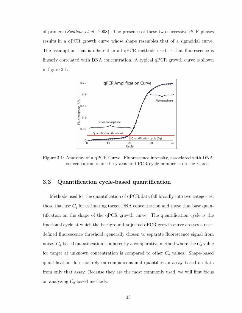
of primers (Swillens et al., 2008). The presence of these two successive PCR phases

results in a qPCR growth curve whose shape resembles that of a sigmoidal curve.

The assumption that is inherent in all qPCR methods used, is that fluorescence is

linearly correlated with DNA concentration. A typical qPCR growth curve is shown

in figure 3.1.

0

0.05

0.1

0.15

0.2

0.25

0 10 20 30 40

Quantification threshold

Quantification cycle (Cq)

Plateau phase

Exponential phase

Cycle

Flu

ore

scen

ce (A

FU)

qPCR Amplification Curve

Figure 3.1: Anatomy of a qPCR Curve. Fluorescence intensity, associated with DNAconcentration, is on the y-axis and PCR cycle number is on the x-axis.

3.3 Quantification cycle-based quantification

Methods used for the quantification of qPCR data fall broadly into two categories,

those that use Cq for estimating target DNA concentration and those that base quan-

tification on the shape of the qPCR growth curve. The quantification cycle is the

fractional cycle at which the background-adjusted qPCR growth curve crosses a user-

defined fluorescence threshold, generally chosen to separate fluorescence signal from

noise. Cq-based quantification is inherently a comparative method where the Cq value

for target at unknown concentration is compared to other Cq values. Shape-based

quantification does not rely on comparisons and quantifies an assay based on data

from only that assay. Because they are the most commonly used, we will first focus

on analyzing Cq-based methods.

33

3.3.1 Absolute quantification with the Cq standard curve

Cq standard curve quantification was the method first used for estimating target

DNA concentration from qPCR data (Higuchi et al., 1993). This method involves

interpolating the absolute initial target DNA amount, D0, from a Cq standard curve,

based on the Cq value for a target at unknown concentration. Typically, a Cq stan-

dard curve is constructed from qPCR assays conducted on a 10-fold dilution series

that spans the range of possible target DNA concentrations in unknown samples.

Constructing a Cq standard curve for quantification involves performing qPCR on a

dilution series with known amounts of target DNA as shown in figure 3.2A, plotting

Cq vs. Log(target concentration) as shown in figure 3.2B, and interpolating using the

resulting curve to quantify target DNA from the Cq of an unknown sample. Quanti-

fying qPCR data using a Cq standard curve results in an absolute estimate of DNA

target concentration.

3 4 5 6 7 8 95

10

15

20

25

10 20 30 40

0.5

1.0

1.5

2.0

A B

Log(Copy Number)

Qua

ntifi

catio

n C

ycle

(Cq)

Cycle

Fluo

resc

ence

(AFU

)

Figure 3.2: Creation of the Cq standard curve. (A) Quantitative PCR data from as-says performed in duplicate on 10-fold serial dilutions of a target withcopy number ranging from 5x108 (far left) to 5x103 (far right). (B) Thequantification cycles (Cq) for these assays are plotted vs. Log(copy num-ber) on a Cq standard curve.

It was shown by Rasmussen (2001) and further detailed by Rutledge and Cote

(2003) that the value for amplification efficiency can be obtained from the Cq stan-

dard curve. Amplification efficiency here is assumed to be a constant value, E, that

34

determines the rate at which the target DNA is amplified. The relationship between

DNA concentration at cycle n, Dn, and E is given as:

Dn = D0(1 + E)n (3.1)

By taking the logarithm of (3.1), we obtain the following formula:

log(Dn) = log(D0) + n log(E + 1) (3.2)

Setting n to the threshold cycle, Cq, we obtain:

log(DCq) = log(D0) + Cq log(E + 1) (3.3)

The Cq standard curve plots log(D0) vs. Cq. By putting (3.3) into the familiar form

of a linear equation (y = mx+ b), where x = Cq and y = log(D0), we obtain:

log(D0) = −Cq log(E + 1) + log(DCq) (3.4)

where the slope is − log(E + 1). Amplification efficiency can thus be expressed as:

E = 10−slope − 1 (3.5)

It is important to note that the mathematical formulae just presented assume that

amplification efficiency is constant throughout the “exponential amplification” phase

of PCR. This is a widespread belief in the biological community and this assumption

underlies many methods used for quantification of qPCR data (Cikos and Koppel ,

2009). It is also important to note that Cq standard curve quantification does not rely

on the assumption of constant amplification efficiency, although assuming constant

amplification efficiency allows (3.1)–(3.5) to be used to analyze Cq standard curves.

35

The only assumption that Cq standard curve quantification relies on is that the shape

of the qPCR growth curve is identical until the threshold such that changes in initial

DNA concentration only shift this curve to the left or right.

3.3.2 Relative quantification

In order to avoid the laborious construction of a Cq standard curve, relative quan-

tification methods have been developed that allow researchers to analyze gene expres-

sion of a target-gene relative to the expression of a so-called housekeeping gene. These

methods involve measuring both target gene expression and reference gene expression

in both an experimental sample (sample) and a control sample (control), for a total

of four conditions. To analyze such data, a ratio of relative expression is calculated

based on differences in the quantification cycle. The first quantification method for

analyzing relative gene expression data was developed by Applied Biosystems and is

based on the following formula:

Ratio = 2−(∆Cqsample−∆Cqcontrol

) = 2−∆∆Cq (3.6)

where the first term in the exponential represents the difference between Cq values for

target and reference genes in the experimental sample, and the second term represents

this difference in the control sample. Amplification efficiency for both target and

reference genes is assumed to be 1 throughout PCR, for perfect doubling of DNA at

every cycle. This method is called the ∆∆Cq method.

The ∆∆Cq method method was later refined by Pfaffl (2001) to account for

differences in amplification efficiency between target and reference genes as follows:

Ratio =(1 + Etarget)

∆Cqtarget (control−sample)

(1 + Eref )∆Cqref(control−sample)

(3.7)

where both target and reference genes have constant, but different, amplification

36

efficiencies. Note that if there is no difference in Cq values for the reference gene, the

denominator is equal to 1.

The relative quantification methods described in (3.6) and (3.7) depend on the

assumption of constant amplification efficiency. The value for amplification efficiency

used in these formulae can be obtained from a Cq standard curve using the relationship

in (3.5) or by fitting an exponential model with constant amplification efficiency, as

in (3.1), to qPCR growth curves as proposed by Tichopad et al. (2003).

3.4 Absolute quantification by model-fitting

Now that we have reviewed Cq-based quantification methods, which are the most

widely used quantification methods in the biological community, we will analyze the

more recently developed shape-based quantification methods. Curve-fitting methods

for quantification of qPCR data were first introduced by Weihong Liu and David

Saint. In 2002, they introduced both exponential-fitting (Liu and Saint , 2002b) and

sigmoidal curve-fitting (Liu and Saint , 2002a). These two classes of models are still

the most widely for qPCR quantification by curve-fitting, however, models derived

from the molecular events occurring during qPCR (i.e., mechanistic models) have

been recently used for quantifying qPCR data (Smith et al., 2007; Boggy and Woolf ,

2010). We will now explore the assumptions that underly fitting qPCR data with

each of these types of models.

3.4.1 Exponential model-fitting

The exponential model is often the model of choice for qPCR data fitting because

Cq standard curves suggest an exponential amplification mechanism for PCR. Expo-

nential models used for qPCR quantification assume that amplification efficiency, E,

is constant at every qPCR cycle, so that in order to calculate the amount of target

DNA at cycle n, one would multiply the DNA at cycle (n− 1) by the multiplicative

37

factor (E + 1). The formula for calculating the amount of DNA at cycle n is given

by (3.1):

Dn = D0(1 + E)n (3.1)

Because fluorescence is linearly correlated with DNA concentration fluorescence as a

function of cycle is given as:

Fn = F0(1 + E)n + Fb (3.8)

where Fb is a background fluorescence in the reaction. This is the model that is fit to

qPCR data in order to obtain values for the parameters F0, E, and Fb. An example

fit of an exponential to qPCR data is shown in figure 3.3.

10 20 30 40

0.5

1.0

1.5

2.0

Cycle

Fluo

resc

ence

(AFU

)

Figure 3.3: Example fit of an exponential to qPCR data.

Amplification efficiency is not truly constant throughout PCR, because if it were

there would be no plateau phase. It is therefore crucial, when fitting qPCR data with

an exponential model, to choose an appropriate cutoff value at which to truncate

the data to be fitted. Tichopad et al. (2003) proposed that the maximum of the

growth curve second derivative represents the end of exponential amplification. This

is a reasonable approach because the exponential model predicts that the second

derivative monotonically increases with increasing cycle number, so when a maximum

38

value of the second derivative is reached, the behavior of the data is not consistent

with the model.

The exponential model is a reasonable approximation of qPCR behavior in the

so-called “exponential” region, under the assumption that amplification efficiency is

constant. We will analyze the validity of this assumption in the discussion section.

We now turn our attention to another type of model used for fitting qPCR data—the

sigmoidal model.

3.4.2 Sigmoidal model-fitting

The sigmoidal model is an empirical model that simulates the entire qPCR growth

curve, though there are potential drawbacks to this. The rationale for using the

sigmoidal model is that it correctly predicts declining amplification efficiency after

the initial log–linear phase of PCR and may thus be a more accurate model of PCR

than the exponential model. The sigmoidal function is an empirical model of qPCR,

however, and although it simulates the shape of the second phase of the qPCR growth

curve, it is possible that it does not describe qPCR behavior in the initial phase of

qPCR. This is especially true for the four-parameter sigmoidal model that was first

used for fitting qPCR data (Liu and Saint , 2002a; Rutledge, 2004), because this model

assumes that data are symmetric about the cycle with half-maximum fluorescence,

when this is rarely the case in reality (Swillens et al., 2008). The model proposed by

Liu and Saint (2002a) is:

F =Fmax

1 + e−(n−n1/2)

k

(3.9)

An example of this model fit to data is shown in figure 3.4

There have been two distinct approaches taken to improve the fit of the sigmoidal

model to asymmetric qPCR data. Rutledge and Stewart have developed a method

termed “linear regression of efficiency” (LRE) that excludes early and late cycle data

from the data to be fitted, to ensure a good fit of the data (Rutledge and Stewart ,

39

10 20 30 40

0.5

1.0

1.5

Cycle

Fluo

resc

ence

(AFU

)

Figure 3.4: Example fit of the Liu and Saint (2002a) sigmoidal model to qPCR data.

2008a,b). The other approach for improving the fit of the sigmoidal model to qPCR

data has been to introduce a fifth parameter to account for asymmetry in qPCR data

(A. Spiess , 2008). Although these increasingly sophisticated sigmoidal model–fitting

methods most often result in better fits of qPCR data, they do not necessarily result

in more accurate quantification of qPCR data, because these empirical methods do

not necessarily simulate qPCR behavior before the qPCR signal increases above noise

(Boggy and Woolf , 2010).

3.4.3 Mechanistic model-fitting

An alternative model–fitting quantification method to empirical model–fitting in-

volves the use of a mechanistic model of qPCR for fitting qPCR data. Rather than

fitting qPCR data with a mathematical function that empirically fits qPCR data,

mechanistic model–fitting aims to quantify qPCR data by using a model that ac-

counts for the underlying molecular events that occur during qPCR. The rationale

for using a mechanistic model for quantifying qPCR data is that in addition to fitting

later cycle data, an appropriate mechanistic qPCR model will more accurately model

qPCR in the cycles before qPCR signal increases above the level of noise.

Until the development of MAK2 (Boggy and Woolf , 2010), which will be further

40

discussed in chapter IV, there has been only one report of a mechanistic model be-

ing applied to fitting qPCR data in order to quantify it (Smith et al., 2007). The

mechanistic model developed by Smith et al. (2007) is applicable to quantifying data

collected from TaqMan qPCR assays. This model is heretofore referred to as the

TaqMan model.

The TaqMan model assumes:

• Primer binding and DNA strand reannealing compete during the anneal step

• Polymerase binding and DNA synthesis occur concurrently with these processes

• DNA synthesis by polymerase can be treated as a single step

• DNA melts completely at the melt step of PCR

• DNA polymerase concentration is non-limiting throughout qPCR

• All DNA is double-stranded at the end of the anneal/extension step

3.5 Discussion

Quantification of qPCR data depends on assumptions about the underlying be-

havior of qPCR. We have just explored the assumptions underlying different qPCR

quantification methods. These assumptions are summarized in table 3.1. We now

turn our attention to analyzing the validity of these assumptions.

Quantification Method AssumptionsCq standard curve Conserved shape of growth curve until thresholdRelative quantification Constant amplification efficiency until thresholdExponential curve–fitting Constant amplification efficiency in log–linear phaseSigmoidal curve–fitting Sigmoidal amplification throughout qPCRTaqMan model–fitting Non-limiting polymerase throughout qPCR

Table 3.1: Underlying assumptions for various qPCR quantification methods.

41

3.5.1 Analysis of the assumption of conserved growth curve shape until

threshold, independent of starting target concentration

This assumption is most often valid, which is why the Cq standard curve is the

most accurate method for quantifying qPCR data. There are, however, cases where

this assumption is not valid. For example, dilutions of samples obtained in the pres-

ence of PCR inhibitors may not exhibit an identical shape for the qPCR growth curve

because the inhibitors would be diluted along with the target DNA (Rutledge and

Stewart , 2008b). In such cases, quantification by model–fitting with an appropriate

model may outperform quantification by Cq standard curve, in terms of quantification

accuracy.

3.5.2 Analysis of the assumption of constant amplification efficiency

This assumption follows from the linearity of the Cq standard curve. Because

plotting Cq vs. the logarithm of initial target concentration appears linear, it is

reasonable to assume that amplification follows the exponential relationship (3.1).

The linearity of the Cq standard curve, however, is misleading. Analysis of the mass

action kinetics of the log–linear phase of PCR reveals that the polymerase chain

reaction does not achieve perfect doubling of target DNA at every cycle because

DNA synthesis by DNA polymerase competes with reannealing of target DNA strands

(Boggy and Woolf , 2010). Strand reannealing occurs to a greater extent as target

concentration builds up, so that amplification efficiency of PCR is in constant decline.

The amplification efficiency that can be obtained from a Cq standard curve as shown

in (3.4) is actually an “effective” amplification efficiency.

To analyze the relationship between the effective amplification efficiency, and the

varying amplification efficiency, we first define the relationship between the target

42

DNA concentration at cycle n, Dn and at cycle n-1, Dn−1:

Dn = (En + 1)Dn−1 (3.10)

The relationship between Dn and D0 is then:

Dn = D0

n∏i=1

(Ei + 1) (3.11)

Relating this equation for Dn to Dn in (3.1), we have:

D0(E + 1)n = D0

n∏i=1

(Ei + 1) (3.12)

where E is the effective amplification efficiency and Ei is the amplification efficiency

for cycle i. Thus, amplification is nearly exponential, but amplification efficiency

varies slightly from cycle to cycle. However, the effective amplification efficiency

obtained from a Cq standard curve is often a good approximation. On the other hand,

amplification efficiency values obtained by fitting qPCR data with an exponential

curve will be most influenced by later qPCR cycles, and thus provide an artificially

low value for early amplification efficiency.

3.5.3 Analysis of the assumption of sigmoidal amplification

The assumption that DNA amplification is sigmoidal neglects the molecular be-

havior that leads to the sigmoidal shape of the qPCR growth curve. The plateau

phase of qPCR occurs due to saturation of DNA polymerase and thus, data collected

during this stage is much less informative than data collected during the log–linear

phase of qPCR. The most important region to describe well is the region where signal

is dominated by noise. Sigmoidal curve–fitting, however, often fits later cycle data

better than data collected during the log–linear phase of qPCR so that qPCR be-

43

havior in the noise–dominated region would not be simulated well by the “best-fit”

sigmoidal model. The only reasonable approach to accurately describe the region of

the qPCR curve dominated by noise is to use an appropriate mechanistic model of

PCR.

3.5.4 Analysis of the assumption of non-limiting polymerase

The assumption of non-limiting polymerase concentration significantly simplifies

the mechanistic model of PCR so that primer elongation to a new complete strand of

DNA can be treated as a single-step. Without this assumption, fitting a mechanistic

model to qPCR data would be extremely difficult because the kinetics of DNA poly-

merase would have to be explicitly modeled, thus introducing more parameters to

optimize over. Following the non-limiting polymerase assumption, it can be assumed

that any ternary complex (i.e. DNA polymerase complexed with primer–template

hybrid) that forms ultimately results in a new strand of DNA being synthesized. The

non-limiting polymerase assumption thus depends on low levels of DNA being present

in the reaction so that polymerase does not saturate.

Smith et al. applied the TaqMan model to fitting qPCR data throughout qPCR,

so that the TaqMan model was fitted to data in regions where the model is not valid.

Although the TaqMan model is an improvement relative to empirical models because

there is some theoretical justification to their methods, the assumption of non-limiting

polymerase throughout qPCR is problematic and leads to some invalid conclusions.

In this model, consumption of probe or primer (rather than enzyme saturation) leads

to the saturation behavior of qPCR, so that the amount of initial target DNA can be

estimated from the height of the plateau.

Smith et al. noticed that calculated values for starting target concentration were

most often underestimated by their model. This is probably because the TaqMan

model assumes completion of DNA synthesis at every step, while this is not the

44

case in reality, due to saturation of enzyme. The faulty assumption of non-limiting

polymerase in later cycles of qPCR leads to an artificially high calculated amplification

efficiency, so that estimated target abundance would be calculated to be artificially

low. Although there are clearly limitations to the TaqMan model, the model most

often predicted target abundances within an order of magnitude of the known starting

concentration, thus validating the use of a mechanistic model for qPCR quantification.

3.6 Conclusion

In this chapter, I have examined the assumptions that underly various methods

of quantifying qPCR data, and the validity of these assumptions. The most com-

mon assumption about qPCR is that amplification efficiency is constant until the

quantification cycle is reached. Although this assumption is invalid, the effective am-

plification efficiency obtained from a Cq standard curve often approximates qPCR

behavior fairly well. The assumption of sigmoidal amplification is problematic be-

cause fitting qPCR data with a sigmoid assigns importance to the least meaningful

data in the plateau phase. Finally, the assumption of non-limiting polymerase con-

centration is useful when fitting qPCR data with a mechanistic model, however, the

limitations of this approach must be recognized for predictions to be quantitatively

accurate.

45

CHAPTER IV

Accurate quantification of qPCR data using a

mechanistic model of PCR

4.1 Introduction

Chapter III provided a critical review of the various methods used for quantifying

qPCR data. As has been suggested by others, the shape of a single qPCR ampli-

fication curve should be sufficient to uniquely determine initial DNA concentration

in a sample (Liu and Saint , 2002b,a; Rutledge, 2004; Smith et al., 2007; Rutledge

and Stewart , 2008a). In practice, however, the available single-assay qPCR analysis

techniques have been less accurate than the gold standard technique of Cq standard

curve calibration (Cikos and Koppel , 2009).

In this chapter, I show that a 2-parameter mechanistic model of PCR, called

MAK2 (for Mass Action Kinetic model with 2 parameters), quantifies DNA samples

from a single qPCR assay as accurately as Cq standard curve calibration, which

requires multiple assays for quantification. Because MAK2 is a mechanistic model

rather than an empirical model, quantifying qPCR data with MAK2 requires no

assumptions about the amplification effiency of a qPCR assay. Furthermore, whereas

Cq quantification uses a single datapoint in the qPCR curve for quantification, MAK2

is fit to measurements across many amplification cycles, thereby reducing the influence

46

of detection noise on estimates of DNA concentration.

4.2 MAK2 is derived from the mass action kinetics of PCR

Assuming that both primers and both target DNA strands can be treated identi-

cally, PCR can be described by the reactions (2.33)–(2.36):

S + PkPS−−−⇀↽−−−k−PS

PS (2.33)

PS + EkE−−⇀↽−−k−E

PSEkcat−−→ D (2.34)

S + SkD−→ D (2.35)

D + EKED−−−⇀↽−−− DE (2.36)

Assuming that all double-stranded DNA melts apart during the melt step of PCR,

these reactions can be translated to the coupled system of equations, (2.37)–(2.45):

d[S]

dt= −kPS[P ][S] + k−PS[PS]− kD[S]2 (2.37)

d[P ]

dt= −kPS[P ][S] + k−PS[PS] (2.38)

d[PS]

dt= kPS[P ][S]− k−PS[PS]− kE[PS][E] + k−E[PSE] (2.39)

d[PSE]

dt= kE[PS][E]− k−E[PSE]− kext[PSE] (2.40)

d[D]

dt= kext[PSE] +

1

2kD[S]2 (2.41)

[D]t=0 = [PS]t=0 = [PSE]t=0 = 0 (2.42)

[S]t=0 = [S]0 (2.43)

[E]t=0 = [E]0 (2.44)

[E]0 = [E] + [PSE] +KED[D][E] (2.45)

47

The initial condition (2.46), that links consecutive cycles, also applies:

[S]t=0,n+1 = 2[D]t=end,n (2.46)

These equations fully describe PCR, with the following assumptions:

1. Errors occurring during PCR can be neglected

2. The complementary DNA strands S1 and S2 can be treated identically as S

3. Primers for S1 and S2, P1 and P2 respectively, can be treated identically as P

4. Off-target effects of PCR primers can be neglected

5. Thermally-induced degradation of DNA polymerase can be neglected

6. Strand elongation is considered as a single step, rather than as a series of single

nucleotide additions

7. Reactions occurring during the anneal/elongation phases go to completion

8. All double-stranded DNA melts at the high temperature step of PCR

There is no analytical solution to (2.37)–(2.45), and simulation of qPCR involves

numerically integrating the ODEs (2.37)–(2.41). Unfortunately there are too many

parameters in these equations to optimize over when fitting qPCR data, so that

attempting to fit qPCR data with (2.41) results in overfitting of the data so that non-

unique solutions are obtained for key parameters such as D0, the amount of target

DNA before PCR is performed.

To find a mechanistic model of PCR that could be applied to fitting to qPCR data,

I applied the assumption that primers and polymerase are in non-limiting concentra-

tions (heretofore referred to as the non-limiting assumption). Under this assumption

48

we can neglect the reverse reactions in (2.33) and (2.34), by Le Chatelier’s princi-

ple, because the excess primer and polymerase result in the forward reactions being

favored. Additionally, the non-limiting assumption allows the dynamic behavior of

primer and polymerase to be neglected. Thus, the reactions (2.33)–(2.36) are simpli-

fied to:

Ska−→ PSE

kext−−→ D (4.1)

S + Skb−→ D (4.2)

If it is now assumed that elongation is the rate–limiting step, it follows that PSE

formation competes with reannealing and any PSE that forms is converted to dsDNA

by the action of DNA polymerase. Thus reactions (4.1) and (4.2) can be further

simplified to:

Ska−→ D (4.3)

S + Skb−→ D (4.2)

where equations (4.3) and (4.2) describe the competition between a first-order reaction

for strand synthesis and a second-order reaction for rehybridization, respectively.

From these reactions, performing the mathematical analysis carried out in appendix

A results in the derivation of MAK2:

Dn = Dn−1 + k ln(1 +Dn−1

k) (4.4)

where Dn represents the amount of double-stranded DNA following cycle n. In equa-

tion (4.4), Dn is recursively dependent on Dn−1, the amount of D from the previous

cycle. The characteristic PCR constant k determines the rate of DNA accumulation

during PCR. D0, and k are the only two adjustable parameters that determine Dn

49

values at every PCR cycle. These parameters have distinct effects on the shape of the

MAK2 curve; changing the value of D0 shifts the curve right or left while changing

the value of k changes the slope of the curve, as shown in Fig. 4.1.

0 2 4 6 8 10 12 140.0

0.2

0.4

0.6

0.8

1.0

Cycle

Dn (

arbi

trarr

y un

its)

D0=10-2 k = 0.5

Increasing k

Increasing D0

D0=10-3 k = 0.5

D0=10-4 k = 0.5

D0=10-3 k = 0.05

D0=10-3 k = 0.005

Figure 4.1: Simulated MAK2 curves with varying D0 and k values. Curves are labeledwith parameter values. Increasing D0 shifts the MAK2 curve to the left,while increasing k increases the slope of the MAK2 curve.

4.3 Analysis of assumptions applied in the derivation of MAK2

Following the development of any theoretical model of a process, the validity of

the assumptions made in formulating that model must be analyzed in order to ensure

that the foundation of the model is on solid ground. Here, we justify each assumption

made in deriving MAK2, beginning with the non-limiting assumption which asserts

that primers and polymerase are in excess and do not limit the rate of reaction.

The non-limiting assumption is valid for early cycles of PCR before target DNA

concentrations rise to concentrations comparable to those of polymerase and primers.

When DNA concentrations rise to the level of polymerase, the enzyme becomes satu-

rated and cannot efficiently process new strands of DNA. When DNA concentrations

rise to the level of primers, the forward process in equation (2.33) is no longer fa-

50

vored over the reverse process and the effects of changing primer concentration must

be considered. A much more complex model is necessary for modeling PCR when

primers and polymerase are limiting, because reaction kinetics change dynamically

in response to changes in primer and polymerase concentration. The limiting effects

of primers and polymerase contribute to late-cycle PCR behavior, such as the onset

of the plateau phase of PCR where very little new DNA is generated. MAK2 is

therefore only applicable to early cycles of PCR where limiting effects of primers and

polymerase can be neglected.

As will become evident, the non-limiting assumption provides critical justification

for all other assumptions made in the derivation of MAK2 except assumptions 1 and

8. While the validity of assumptions 2-7 coincides with validity of the non-limiting

assumption, assumptions 1 and 8 are valid for all cycles of PCR.

Assumption 1: Errors occurring during PCR can be neglected

This assumption is valid when using a non-error prone polymerase. Most commercially-

available DNA polymerases used for quantitative PCR have low rates of introducing

wrong bases (errors) into DNA product. Error prone polymerases that introduce er-

rors to DNA product (useful in methods such as directed evolution) should not be

used for quantitative PCR.

Assumptions 2 and 3: PCR primers and target strands can be treated

identically

These assumptions follow from the assumption that both primers are in excess

(thus favoring PS formation over PS dissociation by Le Chatelier’s principle) and the

assumption that the forward rate for primer-substrate hybridization is independent

of sequence (see references Gevertz et al. (2005); Mehra and Hu (2005)).

Secondary structure in target strands and primers may affect the dynamics of

51

primer hybridization differently for each target strand, so that target strands act dif-

ferently during the course of the reaction. Although secondary structure can hinder

primer hybridization, the excess amount of primer will still drive primer and strand

toward PS formation by Le Chatelier’s principle. Given the assumption that all

reactions go to completion (assumption 7, which follows from the non-limiting as-

sumption), all single-stranded DNA will end up as double-stranded DNA at the end

of the cycle, and both target strands can therefore be treated identically at the end

of each cycle, which is the time-point modeled by MAK2.

Assumptions 4 and 5: Primer off-target effects and polymerase degrada-

tion can be neglected

These assumptions follow from the non-limiting assumption. If primers are in

excess, removal of free primer by off-target hybridization will not have a noticeable

effect on the reaction dynamics. Likewise, if polymerase is in excess, a small amount of

thermally-induced degradation will not have a noticeable effect on reaction dynamics.

Assumption 6: Strand elongation can be considered as a single step

This assumption follows from the assumption that all reactions go to completion

(assumption 7, which follows from the non-limiting assumption). If the elongation

process goes to completion, there are no partially elongated strands remaining at the

end of the elongation step of PCR. Therefore, it is unnecessary to treat elongation

as the series of single nucleotide additions that it is in reality, and elongation can be

approximated as a single step.

52

Assumption 7: Reactions occuring in the anneal/elongation phases go to

completion

This assumption follows from the non-limiting assumption because when primers

are in excess, any single-stranded DNA that does not reanneal to form dsDNA will

form PS through primer hybridization (PS formation is favored over PS dissociation

by Le Chatelier’s principle); and because the polymerase is not saturated with PS

substrate, it is able to complete the elongation reaction during the elongation phase

of PCR. Because the elongation reaction is the rate-limiting step in the production

of a new strand of DNA, all other reactions can be assumed to go to completion.

Assumption 8: All double-stranded DNA melts at the high temperature

step of PCR

This assumption allows the starting amount of ssDNA for cycle n to be related

to the amount of dsDNA after cycle n-1, providing the link between consecutive

cycles. This assumption is valid when the high temperature step of PCR incubates

the reaction at a temperature much higher than the melting temperature of the target

DNA for a sufficient amount of time. Using the protocol for the high temperature

step suggested by the polymerase manufacturer is likely sufficient for this assumption

to be valid.

Practical implications of the non-limiting assumption for PCR analysis

One consequence of the non-limiting assumption is that the actual concentrations

of primer and polymerase are irrelevant to quantification by MAK2. This attribute

of MAK2 is beneficial because enzyme manufacturers typically provide polymerase

concentrations in terms of arbitrary units instead of SI units, so that modeling con-

centration dependent behavior of polymerase can be difficult.

Another consequence of the non-limiting assumption is that MAK2 is applicable to

53

fitting a limited amount of qPCR data. The slope of a qPCR curve initially increases

with each cycle until an inflection point is reached, at which point the slope gradually

decreases until it is flat. MAK2, on the other hand, predicts that the slope of the

qPCR curve increases constantly. This can be seen if equation (4.4) is rewritten as:

Dn −Dn−1 = k ln(1 +Dn−1

k) (4.5)

to obtain the first-derivative of D with respect to cycle. The expression on the right-

hand side increases monotonically with increasing values of Dn−1. Because MAK2

does not predict an inflection point in the qPCR curve, it is no longer an accurate

model when the inflection point is reached in qPCR data. Analysis of qPCR data

reveals that the inflection point is reached soon after the maximum slope increase

occurs. Thus, the cycle with the maximum slope increase, relative to the previous

cycle, is used as the cutoff point for MAK2-fitting. Experimenting with various cutoff

cycles has indicated that setting the cutoff one or two cycles above or below this cycle

does not significantly affect MAK2 concentration predictions.

4.4 MAK2 models the exponential growth phase of PCR

MAK2 can be used for fitting qPCR fluorescence data when Dn in equation (4.4)

represents the fluorescence associated with dsDNA at cycle n. There is often a back-

ground fluorescence in qPCR data that is independent of signal associated with target.

This background fluorescence is due to fluorescence produced by the reaction system

itself, either by plastics or reagents (Cikos and Koppel , 2009). In model-fitting ap-

proaches to quantifying qPCR data, the fluorescence is typically assumed to be com-

posed of signal and a background fluorescence (Liu and Saint , 2002a; Rutledge, 2004;

Rutledge and Stewart , 2008a; Tichopad et al., 2003; A. Spiess , 2008). Similarly, for

MAK2-fitting of qPCR data, fluorescence is background adjusted by the parameter,

54

Fb as follows:

Fn = Dn + Fb (4.6)

where Fb represents constant background fluorescence and Fn is the MAK2-predicted

fluorescence at cycle n, the variable used for fitting qPCR fluorescence data.

Due to assumptions made in deriving MAK2, the model is applicable only to

qPCR data obtained before primer depletion and enzyme saturation are significant

effects. Therefore, in my use of MAK2, I have truncated the data to the cycle with

the maximum slope increase, relative to the previous cycle. Truncation of the data to

be fitted is justified (indeed necessary) based on mechanistic considerations and not

based on statistical classification of outliers as in some qPCR model-fitting methods

(Rutledge, 2004; Rutledge and Stewart , 2008a; Tichopad et al., 2003). The region of

data over which MAK2 is applicable is often referred to as the exponential growth

phase of PCR. An example of an optimized fit of MAK2 to qPCR data is shown in

Fig. 4.2.

0 5 10 15

0.20

0.25

0.30

0.35

0.40

0.45

0.50

Cycle

Fluo

resc

ence

(afu

)

0 10 20 30 400.0

0.5

1.0

1.5

Figure 4.2: Optimized fit of MAK2 (solid line) to data (points). The gray insetdepicts the full data range with the MAK2 fit overlaid. The large curveis a blown up view of the white box in the inset.

55

4.5 MAK2 predicts declining amplification efficiency

PCR amplification efficiency is often used as a parameter for quantifying target

DNA amount from qPCR data. Amplification efficiency is defined on a cycle-by-cycle

basis (Liu and Saint , 2002a) as:

En =Dn −Dn−1

Dn−1

(4.7)

where D is fluorescence due to dsDNA. Applying the MAK2 expression (4.4) to the

amplification efficiency expression (4.7) yields:

En =k ln(1 + Dn−1

k)

Dn−1

(4.8)

From this expression, amplification efficiency is dependent on DNA concentration,

though not linearly as has been previously proposed (Rutledge and Stewart , 2008a).

Furthermore, amplification efficiency monotonically decreases as DNA concentration

increases, in contrast with the assumption that amplification efficiency is constant be-

low the quantification threshold. This assumption of constant amplification efficiency

has been the foundation for the development of Cq quantification methods such as

the relative quantification method developed by Pfaffl (2001).

4.6 MAK2 fitting quantifies qPCR data as accurately as Cq

standard curve calibration

To determine how accurately MAK2 fitting performs relative to other qPCR quan-

tification methods, I analyzed three independently generated qPCR dilution series

by MAK2 fitting, Cq standard curve calibration, exponential curve fitting (Liu and

Saint , 2002b), and sigmoidal curve fitting with 4 and 5 parameter log-logistic func-

tions (A. Spiess , 2008). The resulting log-log plots of estimated vs. known target

56

amount are shown in the panels of figure 4.3. I generated the first of the three datasets,

shown in figure 4.3A, as described in appendix B. The other two datasets used for

demonstrating MAK2 were chosen from datasets freely available to researchers in the

R package qpcR (Ritz and Spiess , 2008). These datasets were assumed to be repre-

sentative of standard qPCR data because they are included as example datasets in

the qpcR package for the purpose of demonstrating various model-fitting procedures

for quantification of qPCR data.

Fitting accuracy was evaluated using the R2 coefficient of determination for linear

models that represents the proportion of the variability in the dependent variable that

can be explained by the regression equation. R2 is a metric of the goodness of fit of the

best fit line, with a value of 1 indicating perfect correlation and a value of 0 indicating

no correlation. By analysis of R2 values, the plots in Fig. 4.3 demonstrate the

equivalent performance of MAK2 quantification and Cq standard curve quantification,

and the superior performance of these two methods relative to other model-fitting

quantification methods. The third most accurate quantification method was different

for each dilution set, indicating how variable the predictions made by these methods

can be.

The R2 values for MAK2 and Cq were very similar for the datasets analyzed, so

it was hypothesized that these quantification methods are statistically equivalent. In

order to test this hypothesis, these methods were compared using the Bland-Altman

method for comparing two different methods for measuring the same thing (Altman

and Bland , 1983). This method is used in medicine to determine whether a new

measurement method can be reasonably used to replace the current standard mea-

surement method. Briefly, the Bland-Altman method enables one to assess systematic

biases between two measurement methods by analyzing the differences between two

measurements as a function of the mean of these measurements. Performing linear

regression on these variables enables one to test the null hypothesis. For replicated

57

data, this analysis can be performed on the mean of the replicates.

Prior to performing the Bland-Altman analysis to compare MAK2 quantification

and Cq standard curve quantification of the same data, copy number values pre-

dicted by MAK2 and by Cq standard curve, for a given known target copy number,

were averaged. Performing the Bland-Altman analysis resulted in P-values greater

than 0.95 for every data set, providing strong indication that MAK2 quantification

and Cq standard curve quantification can be considered equivalent. Based upon this

finding, it was decided that it is acceptable to report only three significant figures

when reporting the R2 values shown in figure 4.3 although four would be necessary to

highlight the differences between MAK2 quantification and Cq standard curve quan-

tification. Three significant figures are necessary to highlight differences between

these two methods and other quantification methods shown in figure 4.3. Note that

quantification by the Cq standard curve requires the entire dilution series, while esti-

mates made by the other four quantification methods are based on single qPCR runs

at each dilution.

4.7 Discussion

I have demonstrated that fitting qPCR data with a 2-parameter mechanistic model

of PCR, MAK2, quantifies single qPCR assays as reliably as Cq standard curve cal-

ibration for a variety of target sequences and a wide range of concentrations. In

contrast, quantification by fitting qPCR data with an empirical model, such as an

exponential curve or a sigmoidal curve, is not as reliable and accurate quantification

is strongly dependent on PCR conditions used.

Empirical model-fitting methods, such as sigmoidal or exponential curve-fitting,

fail to reliably quantify qPCR data because they are unable to accurately describe

amplification efficiency in early cycles of qPCR where the fluorescence signal is dom-

inated by noise. The model-predicted behavior in these early cycles depends on as-

58

R2=0.999

R2=0.998

R2=0.958

R2=0.540

R2=0.266

02

46

810

12024681012

MA

K2

02

46

810

12024681012

Cq

02

46

810

12024681012

Expo

nent

ial

02

46

810

12024681012

4Pa

ram

eter

Sigm

oid

02

46

810

12024681012

5Pa

ram

eter

Sigm

oid

R2=0.998

R2=0.998

R2=0.943

R2=0.996

R2=0.983

R2=0.994

R2=0.997

R2=0.902

R2=0.488

R2=0.946

02

46

810

12024681012

02

46

810

12024681012

02

46

810

12024681012

02

46

810

12024681012

02

46

810

12024681012

02

46

810

12024681012

02

46

810

12024681012

02

46

810

12024681012

02

46

810

12024681012

02

46

810

12024681012

MA

K2

Cq

Exp

onen

tial

4-P

aram

eter

Sig

moi

d5-

Par

amet

er S

igm

oid

(A)

Dat

aset

ge

nera

ted

w

ith s

ynth

etic

D

NA

n

= 2

(B)

‘rutle

dge’

data

set i

n

R p

acka

ge

‘qpc

R’

n

= 20

(C)

‘reps

’ dat

aset

in

R p

acka

ge

‘qpc

R’

n

= 4

Log (Estimated Number of Template Copies)

Log

(Num

ber o

f Tem

plat

e C

opie

s)

Fig

ure

4.3:

Ass

essm

ent

ofquan

tica

tion

accu

racy

for

five

quan

tica

tion

met

hods

onth

ree

indep

enden

tdat

aset

s.D

atas

ets

(row

sA

-C

wit

hn=

2,n=

20,

and

n=

4re

plica

tes

per

conce

ntr

atio

n,

resp

ecti

vely

)w

ere

quan

tified

by

five

met

hods

(in

colu

mns)

asfo

llow

s:M

AK

2:m

odel

-fitt

ing

wit

hM

AK

2;C

q:C

qst

andar

dcu

rve

calibra

tion

;E

xp

onen

tial

:ex

pon

enti

alcu

rve-

fitt

ing

(Liu

and

Sai

nt,

2002

b);

4-P

aram

eter

Sig

moi

d:

sigm

oidal

curv

e-fitt

ing

(SC

F)

wit

ha

4-par

amet

erlo

g-lo

gist

icfu

nct

ion

(A.

Spi

ess,

2008

);5-

Par

amet

erSig

moi

d:

SC

Fw

ith

a5-

par

amet

erlo

g-lo

gist

icfu

nct

ion

(A.

Spi

ess,

2008

).P

anel

sin

the

figu

reco

nta

inlo

g-lo

gplo

tsof

esti

mat

edvs.

actu

alnum

ber

ofte

mpla

tem

olec

ule

s.T

he

line

at45◦

inea

chplo

tre

pre

sents

the

line

ofag

reem

ent

bet

wee

npre

dic

tion

and

know

nam

ount.

Row

sar

ela

bel

edw

ith

the

sourc

eof

the

dat

a(T

he

qP

CR

grow

thcu

rves

ofco

rres

pon

din

gto

row

Aar

esh

own

infigu

reC

.1an

dth

era

wdat

aar

egi

ven

inta

ble

C.1

).

59

sumptions about amplification efficiency implicit in the model. For example, fitting

qPCR data with an exponential curve implies that amplification efficiency observed

in the log-linear region of the qPCR curve is constant through all early PCR cycles

while fitting with a sigmoidal curve implies that early cycle amplification efficiency

follows a sigmoidal trend. Because these assumptions are not consistent with the

mechanism of PCR, empirical model predictions are less reliable than predictions

made by mechanistic models such as MAK2.

The two parameters in MAK2, D0 and k, are sufficient to accurately describe com-

plex PCR behavior for early cycles of qPCR, where effects such as primer depletion or

polymerase saturation can be neglected. The initial target DNA concentration, D0,

determines where the fluorescence signal rises above noise. The parameter k, repre-

sents the ratio of primer binding and DNA reannealing rate constants and dictates

how amplification efficiency changes at every cycle with increasing DNA concentra-

tion. While k should theoretically remain constant for a given amplicon sequence and

primer set, fitting with MAK2 revealed that this is not always the case (see figure

C.2). The observed variation in k may indicate the presence of unexplained qPCR

effects, but further study is needed to determine its significance.

MAK2 is the first mechanistic model of PCR suitable for quantifying qPCR data

generated with either nonspecific dyes or specific probes. A mechanistic model of

specific probe binding has been developed and used for quantifying qPCR data gen-

erated by hydrolysis probes (Smith et al., 2007). Detailed mechanistic models of PCR

have also been developed and used in simulating PCR (Mehra and Hu, 2005; Gevertz

et al., 2005), however, these models contain many more parameters than MAK2 and

attempting to use these models for fitting qPCR data results in data overfitting and

non-unique solutions for key parameters such as D0. The three parameters used for

fitting MAK2 to qPCR data (k; D0; and background fluorescence, Fb) each affect

the simulated MAK2 curve in orthogonal ways, so that fitting with MAK2 ensures a

60

unique solution for the optimal parameter set.

The approach used in this work reflects a broader trend in systems biology of

trading assay complexity for software complexity. As a well-known example, shotgun

sequencing enables sequencing of large DNA segments using simplified experimental

methods by shifting complexity to sequence reconstruction software. Similarly, the

MAK2 approach enables accurate DNA quantification using significantly less complex

experimental methods by carrying out a more complex, mechanistic software analysis.

As a result, MAK2 provides a robust single assay method for DNA quantification.

61

CHAPTER V

Simplified multiplex qPCR with monochrome

multiplex qPCR and mechanistic data analysis

5.1 Introduction

In chapter II, I discussed the biophysics of quantitative PCR and discussed causes

of the plateau–phase of PCR. The plateau–phase behavior of PCR negatively affects

the quantitativeness of multiplex qPCR, often causing DNA amplification to be biased

toward individual targets in multiplex reactions (Kanagawa, 2003). Consequently,

current approaches for multiplexing qPCR are most applicable to target detection

rather than target quantification because DNA amplification is often biased toward

individual targets in multiplex reactions (Kanagawa, 2003). Furthermore, multiplex

qPCR assays have generally relied on sequence-specific FRET-based probes that re-

quire optimization of reaction conditions to ensure proper target hybridization.

The trial-and-error design and optimization of reaction conditions that is typi-

cally required for multiplex qPCR can be avoided by using sophisticated nucleic acid

software design and simulation tools. These tools aid multiplex probe and primer

design by performing accurate calculations of the thermodynamics associated with

target hybridization, secondary structure formation, and off-target hybridization un-

der assay buffer conditions(SantaLucia and Hicks , 2004). Such tools are useful for

62

designing single target qPCR assays, but become essential for avoiding problematic

DNA interactions as assay complexity increases with more target, probe, and primer

sequences in multiplex reactions.

Although appropriate software tools address much of the complexity associated

with multiplex qPCR assays, they cannot address inherent properties of PCR such

as the DNA concentration-dependent depletion of unbound DNA polymerase. The

depletion of free polymerase in PCR assays leads to the “plateau phase” observed in

the later cycles of qPCR data (Lee et al., 2006). In multiplex reactions, this depletion

also leads to amplification biased toward more abundant DNA targets. Addressing

amplification bias due to polymerase depletion requires a novel approach to multiplex

qPCR.

One such novel approach to multiplex qPCR, the monochrome multiplex qPCR

(MMQPCR) assay, was recently developed by Cawthon (2009). This assay employs

the unique melting behavior of individual target sequences to measure abundance of

two targets using a double-stranded DNA (dsDNA) dye such as SYBR R© Green. An

additional high temperature incubation step during the PCR cycle causes one target

to melt, thus freeing bound DNA polymerase to process less abundant DNA targets,

resulting in the elimination of amplification bias. In theory, the MMQPCR assay

enables researchers to reliably quantify multiple target DNA sequences for nearly the

same cost and effort associated with quantifying a single target in a qPCR assay

using a dsDNA dye. Thus far, however, the method has been demonstrated for only

a limited number of cases where the concentration ratio between targets with low and

high melting temperature (Tm) has been relatively constant. Additionally, MMQPCR

assay throughput is currently limited by quantification cycle (Cq) standard curve

quantification which requires construction of a Cq standard curve to quantify assays

of samples with unknown concentrations. Quantifying MMQPCR data by fitting

with a mechanistic PCR model, such as the MAK2 model I described in chapter

63

IV, eliminates the need for a standard curve and can thus increase experimental

throughput without sacrificing accuracy.

I have performed studies of the MMQPCR assay with two DNA targets at varied

concentrations both to explore the limitations of the MMQPCR assay and to assess

the applicability of the MAK2 model of PCR to reliably quantify multiple targets

from MMQPCR data. In this chapter, I demonstrate that a modified version of the

MAK2 model, called MAK3, can be used to accurately quantify both targets in a

duplex MMQPCR assay, without the use of a standard curve, when the lower Tm

target is at least ten times more abundant than the higher Tm target. Combining the

MMQPCR assay with MAK3 quantification simplifies multiplex qPCR because the

combination enables parallel DNA quantification with a single dye and single color

detection equipment without the use of standard quantification curves.

5.2 Three-dimensional data facilitates optimal MMQPCR data

analysis

In order to explore the limitations of MMQPCR measurement of DNA target

concentrations, I have performed a systematic study using MMQPCR to measure

concentrations of two synthetic DNA targets, A and B, in a range of concentration

combinations. The MMQPCR assay I have performed is a slightly modified version

of the MMQPCR assay performed by Cawthon; rather than obtaining fluorescence

data at two temperatures, I have obtained fluorescence data at many temperatures

following each cycle of PCR after cycle 10. These data were not collected during

the first ten cycles in order to limit early nonspecific amplification that can occur

during extended periods at temperatures favorable to DNA polymerase activity. For

each assay, the data collected after cycle 10 formed a three-dimensional dataset which

could be sliced into real-time melt curves obtained at a given cycle or into individual

64

qPCR growth curves obtained at a given temperature, as shown in figure 5.1.

The three-dimensional dataset shown in figure 5.1a is sliced at cycle 19 to yield

the melt curve shown in figure 5.1b. The trough between temperature derivative

peaks shown reveals that between 81.4 and 82.0◦C, the lower Tm sequence (sequence

A) has melted nearly completely and the higher Tm sequence (sequence B) has not

melted significantly, an observation that was further supported by analysis of multiple

melt curves from various assays. Based upon this observation, 81.4◦C was chosen as

the observation temperature for sequence B. When the three-dimensional dataset

in figure 5.1a is sliced at this temperature, the growth curve shown in figure 5.1c

is obtained. Obtaining detailed three-dimensional data enables analysis of growth

curve data obtained at the optimal temperature for the higher Tm sequence, without

knowing a priori what the optimal temperature is.

Copy numbers for sequences A and B were estimated by fitting a modified version

of the MAK2 model (Boggy and Woolf , 2010), called MAK3, to cycle-dependent fluo-

rescence data obtained at the 64◦C and 81.4◦C incubation temperatures, respectively.

Fitting the 64◦C data resulted in a estimated D0 value for the low Tm sequence A

and fitting the 81.4◦C data resulted in estimated D0 values for the high Tm sequence

B. MAK3 uses an additional parameter, relative to the original implementation of

MAK2, to adjust for sloping background in the data (see appendix D for details).

5.3 MMQPCR is limited by relative abundance of the high

Tm target

To analyze the limitations of the MMQPCR assay, I compared concentration

estimates for targets in MMQPCR assays to concentration estimates for targets, at

identical concentrations, in monoplex qPCR assays. Table 5.1 shows values calculated

for the ratio of MMQPCR-predicted concentration to monoplex qPCR-predicted con-

65

2025

3035

40

0.4

0.5

0.6

0.7

0.8

0.9

Gro

wth

cur

ve a

t 81.

4 o C

MA

K3 F

it

bc

a

b

c

Tem

pera

ture

(o C)

Tem

pera

ture

(o C)

Cycl

eCy

cle

Normalized Fluorescence (AFU)

Fluorescence (AFU)

Fluorescence (AFU)

+++++

+

++++++++++++++++++

++

7980

8182

8384

85

0.2

0.4

0.6

0.8

1.0

Mel

t cur

ve d

ata

(+) a

t cyc

le 1

9

Der

ivat

ive

data

Obs

erva

tion

Tem

p fo

r B

2030

40

Fig

ure

5.1:

Dat

aob

tain

edfr

omth

eM

MQ

PC

Ras

say.

(a)

The

thre

e-dim

ensi

onal

MM

QP

CR

dat

aca

nb

esl

iced

ata

give

ncy

cle

toob

tain

are

al-t

ime

mel

tcu

rve,

orat

agi

ven

tem

per

ature

toob

tain

agr

owth

curv

eat

that

tem

per

ature

.T

he

dat

ash

own

isfr

oman

assa

yw

ith

5x10

8co

pie

sof

sequen

ceA

(low

Tm

)an

d5x

106

copie

sof

sequen

ceB

(hig

hT

m).

(b)

The

mel

t-cu

rve

dat

ash

own

corr

esp

onds

toth

esl

ice

lab

eled

b,ta

ken

atcy

cle

19,

from

the

3Ddat

ash

own

in(a

).T

he

der

ivat

ive

dat

aan

db

est-

fit

Gau

ssia

nfu

nct

ions

for

the

two

der

ivat

ive

pea

ks,

wit

hth

ese

quen

ceA

pea

kat

80.5◦ C

and

the

sequen

ceB

pea

kat

83.0◦ C

,ar

eov

erla

idw

ith

the

mel

tcu

rve

dat

a.(c

)T

he

grow

thcu

rve

show

nco

rres

pon

ds

toth

esl

ice

lab

eled

cta

ken

at81

.4◦ C

from

the

3Ddat

ain

(a).

The

bes

t-fit

MA

K3

curv

eis

over

laid

wit

hth

e81

.4◦ C

grow

thcu

rve

dat

a.

66

centration ([Target]multi : [Target]mono) for both target sequences A and B. This ratio

has an expected value of 1, indicating agreement between monoplex and multiplex

predictions. Significant deviation from a value of 1 for this ratio indicates that the

target in the multiplex reaction cannot be correctly quantified. Analysis of table 1

reveals that sequence B was always quantified correctly regardless of the concentra-

tion of sequence A, but the concentration of sequence A was only quantified correctly

when it was more abundant than sequence B. Deviation from the expected behavior

for the 5x103 copy number condition for sequence B is due to high levels of noise at

this concentration, as observed in figure 5.3. When target concentrations were equal,

the ratio calculated for sequence A was roughly 2, indicating that both sequences are

being accounted for in the estimated D0 value for sequence A. When sequence B was

more abundant than sequence A, on the other hand, the ratio reflects the ([B] : [A])

concentration ratio, indicating that only sequence B concentration is accounted for

in the estimate. The limitations of MMQPCR are further illustrated in figure 5.2.

Figure 5.2a shows representative growth curves for target sequences A and B when

sequence B is at 5x107 copies per well and the copy number of sequence A is at the

specified ratio relative to sequence A (this corresponds to the bottom row of table

1). As expected, the growth curves for sequence B are indistinguishable, regardless of

sequence A concentration, leading to correct estimates of sequence B concentration.

When the ratio ([A] : [B]) is 1:100 or 1:10, the sequence A growth curves cannot be

distinguished. When ([A] : [B]) is 1:1, the growth curve for sequence A is only slightly

distinguishable from the growth curves obtained for ([A] : [B]) ratios of 1:100 and 1:10.

When ([A] : [B]) is 10:1, the sequence A growth curve is clearly distinguishable from

the other sequence A growth curves and there is sufficient data before the sequence

B signal rises to quantify sequence A independently of sequence B.

The trends for the sequence A growth curves closely follow the trends in sequence

B growth curves when the ([A] : [B]) ratio is 1:100, 1:10, or 1:1. This is apparent in

67

Table 5.1: Ratios of MMQPCR-predicted concentration to monoplex qPCR-predictedconcentration for synthetic DNA sequences A and B

[A]multi : [A]monoCopies of Sequence A (low Tm)5x105 5x106 5x107 5x108

5x103 0.88 0.91Copies of (5x103) 0.99 0.95 1.0 0.99Sequence B 5x104 1.0 1.0 0.94(high Tm) (5x105) 1.8 0.97 0.97 1.0

5x106 8.9 2.0 1.2 1.15x107 69 8.4 2.1 1.1

[B]multi : [B]monoCopies of Sequence A (low Tm)5x105 5x106 5x107 5x108

5x103 0.09∗ 0.13∗

Copies of (5x103) 0.11∗ 0.11∗ 0.15∗ 0.23∗

Sequence B 5x104 0.52 0.58 0.61(high Tm) (5x105) 1.5∗ 1.2 1.4 1.5

5x106 0.82 1.0 1.1 1.05x107 0.8 1.0 0.97 0.92

The ratio of MMQPCR-predicted concentration to monoplex qPCR-predictedconcentration was calculated for sequences A and B with the copy numbercombinations shown. The cell color provides a visual representation of this ratio,with white background indicating a ratio lower than 2, gray background indicating aratio between 2 and 10, and black background with white text indicating a ratiogreater than 10. Each assay was performed in duplicate. The parentheses aroundsome copy numbers for sequence B indicate that these samples are unknowns thatare estimated to be near this concentration based on quantification results, as shownin figure 5.3. Asterisks (*) indicate standard error above 25%.

68

10 12 14 16 18 20 22

0.5

1.0

1.5

2.0

2.5

8 10 12 14 16 18 20

0.05

0.10

0.15

0.20

0.25

0.30

0.35

CycleCycle

Fluo

resc

ence

(AFU

)

dF/d

n (A

FU)

a b

10:1 1:11:1001:10

1:1001:10

10:1 1:1

Increasing ratioof [A]:[B]

[B] = 5 x107 copies/reaction

MaximumDerivativeCycle

Figure 5.2: Effect of varying the ratio of sequence A concentration to sequence Bconcentration ([A]:[B]). (a) qPCR growth curves obtained at 64◦C arelabeled with the concentration ratio of [A]:[B] ([low Tm sequence]:[highTm sequence]) in the assay, with [B] at 5x107 copies per reaction. Growthcurves obtained at 81.4◦C (four curves at the bottom right) are indistin-guishable. (b) The growth curve derivatives for the data in (a) are shown.The dashed line indicates the cycle with the maximum derivative valuefor the 81.4◦C curves and the 64◦C curves with [A]:[B] ratios of 1:100,1:10, and 1:1.

the peaks of the growth curve derivative plots shown in figure 5.2b. The sequence A

and sequence B derivative peaks have maximum derivative values at the same cycle

in these cases. This indicates that signal due to sequence B is being observed at both

temperatures because sequence B outcompetes sequence A during amplification. The

derivative peak for sequence A is shifted about three cycles to the left relative to the

peak for sequence B when the ([A] : [B]) is 10:1, indicating that there is sufficient

sequence A signal without significant contribution from sequence B to estimate the

sequence A concentration independently of sequence B.

5.4 MAK3 fitting quantifies MMQPCR data as accurately

as Cq standard curve calibration

To analyze the validity of MAK3 quantification, I compared the accuracy of

MAK3-generated concentration estimates to the accuracy of concentration estimates

69

generated by Cq standard curve quantification. To ensure that MAK3-generated re-

sults for sequence A reflected the actual concentration of sequence A, the derivatives

of the qPCR growth curves obtained at 64◦C and 81.4◦C were analyzed and data with

derivative maxima separated by less than two cycles were not included in the analysis.

Figure 5.3 shows that for both sequences A and B, MAK3 quantification performed

at least as well as Cq standard curve quantification. Because MAK3 quantification

enables estimation of concentration based upon a single assay, MAK3 quantification

increases MMQPCR throughput relative to experiments quantified with a Cq stan-

dard curve.

Based on the Bland-Altman analysis performed in chapter IV, it was concluded

that MAK2 quantification and Cq standard curve quantification could be considered

equivalent methods for quantification of qPCR data. Based on this result, it was

decided that the R2 values shown in figure 5.3 do not need to highlight differences

between MAK3 quantification and Cq standard curve quantification for low Tm target.

To do so would require at least four significant figures. Two significant figures are

enough to highlight differences between MAK3 quantification and Cq standard curve

quantification for the high Tm sequence, so only two significant figures are reported for

R2 values in figure 5.3. The differences between these methods for high temperature

data are likely due to the decrease in signal-noise ratio due to melting of dsDNA.

5.5 Validation of MMQPCR and MAK3 fitting on assays of

a biological system

The results discussed thus far have been generated on a system of synthetic DNA

sequences. To demonstrate the utility of MMQPCR with mechanistic data analysis

in real biological systems, I developed a duplex MMQPCR assay that allows for di-

rect and accurate quantification of cell densities for the fungus, Trichoderma reesei

70

MAK3(64 oC) Cq(64 oC) MAK3(81.4 oC) Cq(81.4 oC)

R2=0.99 R2=0.99 R2=0.97 R2=0.96

3 4 5 6 7 8

3

4

5

6

7

8

3 4 5 6 7 8

3

4

5

6

7

8

5 6 7 8 95

6

7

8

9

5 6 7 8 95

6

7

8

9

Unknowns Unknowns

Log(Copy Number)

Log(

Pred

icte

d C

opy

Num

ber)

Figure 5.3: Accuracy of MAK3-fitting vs. Cq standard curve quantification. Theplots show estimated D0 vs. actual D0 on a log-log scale for data obtainedat 64◦C and at 81.4◦C. The line at 45◦ in each plot represents the line ofagreement between the estimation and known amount. Assays with anunknown concentration for sequence B are indicated by arrows.

and the bacterium Escherichia coli in a T. reesei—E. coli consortium. E. coli—T.

reesei consortia are currently being investigated for use in cellulosic biofuel produc-

tion (Minty, unpublished results). Quantitative PCR measurement of species-specific

gene targets offers a direct, accurate, and sensitive method for quantifying species

composition in a microbial consortium (Smith and Osborn, 2009). By multiplexing

different species-specific qPCR reactions, assay throughput can be increased allowing

for significant cost savings and increases in laboratory productivity.

Prior studies of the T. reesei—E. coli consortium suggest that E. coli cells out-

number T. reesei cells under most growth conditions (Minty, unpublished results),

motivating selection of a low Tm PCR target for E. coli and high Tm PCR target

for T. reesei. For the E. coli target, I chose a sequence conserved amongst all seven

16S rRNA genes in E. coli, while I arbitrarily chose a single-copy gene with high GC

content for the T. reesei target. The choice of a multicopy target in E. coli and

single copy target in T. reesei further ensures a high ratio of low Tm target to high

Tm target.

In order to test if my observations would hold for a biological system, I performed

qPCR assays on mixtures of diluted genomic DNA that was extracted and purified

71

from E. coli and T. reesei monocultures. The two targets had nearly a 10◦C difference

in melting temperature as demonstrated by the representative endpoint melt curves,

from monoplex assays, shown in figure 5.4a. Based on the observed melting profiles, a

temperature of 78◦C was chosen for analyzing the T. reesei target. The targets were

each diluted into three concentrations as shown in figure 5.4b. Each of these dilutions,

for each target, was assayed in monoplex and in duplex with each dilution from the

opposite target. Thus, in addition to monoplex assays, a 9x9 grid of multiplex assays

was performed. This grid was analyzed for agreement between monoplex predictions

and multiplex predictions, as shown in table 5.2. The D0 values for the E. coli target

corresponding to the cells that are not shaded in table 5.2 are plotted in 5.4b, along

with the D0 values predicted from monoplex assays. All D0 values obtained for the

T. reesei target are plotted in figure 5.4b. The data shown in figure 5.4b and in table

5.2 confirm that MMQPCR and MAK3 fitting can be used to quantify both targets

in a duplex reaction when the lower Tm target is ten times as abundant as the higher

Tm target.

Table 5.2: Ratios of MMQPCR-predicted concentration to monoplex qPCR-predictedconcentration for the microbial consortium

[E]multi : [E]monoE. coli DNA (low Tm)

Low Medium HighT. reesei DNA Low 2.0 1.4 1.8∗

(high Tm) Medium 14 1.2∗ 1.1∗

High 140 2.9∗ 0.90∗

[T]multi : [T]monoE. coli DNA (low Tm)

Low Medium HighT. reesei DNA Low 1.4∗ 1.1 0.84(high Tm) Medium 1.1 0.70 0.75

High 1.2∗ 0.73∗ 0.55

The ratio of MMQPCR-predicted concentration to monoplex qPCR-predictedconcentration was calculated for qPCR assays performed on dilutions of the E. coli(E) and T. reesei (T) targets in the combinations shown. The cell color provides avisual representation of this ratio, with white background indicating a ratio lowerthan 2, gray background indicating a ratio between 2 and 10, and black backgroundwith white text indicating a ratio greater than 10. Each assay was performed induplicate. An asterisk (*) indicates standard error above 25%.

72

-10

-9

-8

-7

-6

75 80 85 90

0.20

0.25

0.30

0.35

0.40

0.45

Log(

D0)

Temperature (oC)

Fluo

resc

ence

(AFU

)

a b

Low Medium HighRelative Concentration

T. reesei

T. reeseiE. coli

E. coli

Figure 5.4: Data obtained on the microbial coculture. (a) The representative end-point melt curves shown demonstrate a wide separation between the melt-ing temperatures of the E. coli (E) and T. reesei targets. Based on suchdata, a temperature of 78◦C was chosen for observing the higher Tm T.reesei target. (b) Log(D0) is plotted for the dilutions analyzed for bothtargets. All of the data obtained on the T. reesei target is plotted, whilethe only data plotted for the E. coli target are conditions where the T.reesei target does not significantly contribute to the fluorescence signalobtained at 72◦C.

5.6 Discussion

We have shown that the mechanistic model of PCR, MAK3, can be fitted to data

from an MMQPCR assay with two targets to accurately quantify both targets. The

concentration for the high Tm target sequence in an MMQPCR assay can always

be estimated, regardless of low Tm target abundance, but the low Tm target can be

accurately quantified only when it is more abundant and the high Tm target signal

does not contribute significantly to the data used for low Tm target quantification. I

have found that in order to accurately quantify the low Tm target, the concentration

ratio between low Tm and high Tm targets must be greater than some threshold

value that lies between 1 and 10. Although the low Tm target concentration cannot

be quantitatively estimated when the high Tm target is too abundant, qualitative

information about low Tm target concentration can be obtained by analysis of growth

curve derivative data. Thus, although a numerical concentration estimate for low

73

Tm sequence cannot always be obtained, MMQPCR data provides, at minimum, an

upper bound for the possible range of low Tm target concentration.

Because the MMQPCR assay eliminates amplification bias toward abundant tar-

gets, it may be possible to use this method in applications previously inaccessible to

multiplex qPCR, such as measurement of gene expression. For example, a possible

clinical application of the duplex MMQPCR assay is the simultaneous measurement

of the expression of both genes in a two-transcript gene expression classifier for the

diagnosis and prognosis of human disease (Edelman et al., 2009). More commonly,

the assay may be used for measuring the expression of a gene relative to the expres-

sion of a housekeeping gene. Theoretically, elimination of amplification bias enables

the MMQPCR assay to be scaled up to measuring more target sequences in a single

assay, however, the restrictions on relative target concentrations for quantification

of all targets makes MMQPCR somewhat impractical for more than two targets.

Nevertheless, the quantitatively accurate single-lable multiplexing capability of the

MMQPCR assay, offers advantages in terms of cost, accuracy, and simplicity, relative

to commonly used multiplex qPCR methods.

The methods introduced here expand the applicability of the MAK2 model of PCR

to quantifying data from a multiplex qPCR assay, resulting in higher throughput

and lower cost multiplex quantitative PCR. Fitting MMQPCR data with a slope-

adjusted version of MAK2, called MAK3, increases MMQPCR throughput while

decreasing reagent cost by eliminating the necessity of a Cq standard curve for reliable

quantification of MMQPCR data. I anticipate that the MMQPCR assay combined

with MAK3 fitting will make the benefits of multiplex quantitative PCR more widely

accessible to researchers.

74

CHAPTER VI

Conclusions, Applications, and Future Directions

In this thesis, I used knowledge of the biophysics of PCR to optimize qPCR meth-

ods to minimize cost and complexity of qPCR. By applying simplifying assumptions

to the mass action kinetic model of PCR, I have obtained a simple mathematical

formula, called MAK2, that well describes the exponential phase of qPCR. I have

further applied MAK2–based quantification to data obtained with the monochrome

multiplex qPCR assay, which uses the melting behavior of double-stranded DNA to

perform quantitatively accurate multiplex qPCR. This chapter concludes this thesis

with applications of the methods I have developed and future directions for further

development of biophysics–inspired qPCR technologies.

6.1 Conclusions

In chapter IV, I developed a new mechanistic model for PCR that can be fit to

qPCR data from the exponential phase in order to quantify the qPCR data. The

model relies on the assumption that primers and polymerase are both in excess and

do not limit the rates of reaction. The model, MAK2, is thus applicable to qPCR

data obtained during the exponential phase. Because MAK2 fitting relies on only

two parameters to describe qPCR data (additional parameters adjust for background

signal), there is little risk of over-fitting data and optimal estimated values of initial

75

target concentration are unique. Experimental validation on three-independently

generated datasets showed that MAK2–quantification performed equivalently to Cq

standard curve quantification and superiorly to other model–fitting methods.

In chapter V, the capability of MAK2 quantification was extended to data ob-

tained with the monochrome multiplex qPCR assay, using a slope–adjusted version

of MAK2 called MAK3. This automated analysis of MMQPCR data further in-

creases the throughput of the MMQPCR assay. Because the MMQPCR assay relies

on a single target dominating the signal at a given temperature, however, the ability

of MMQPCR to quantify both targets in an assay is limited to assays where the target

with the lower melting temperature is at least ten times as abundant as the target

with the higher melting temperature. The higher Tm target can always be quantified,

however, and MMQPCR followed by MAK3 quantification provides at least an upper

bound on the concentration of the lower Tm target.

6.2 Applications of MAK2 and automated analysis of MMQPCR

6.2.1 Applications of MAK2

The mass action kinetic model of PCR with two-parameters (MAK2) is a model

of PCR that can be applied to quantify any qPCR data. Possible clinical applications

include, but are not limited to, monitoring the progress of infectious diseases by mea-

suring the concentration of viral or bacterial genes and monitoring cancer treatment

by measuring biomarker levels associated with disease. Because MAK2 can be applied

to any qPCR data, the applications of the model are as diverse as the applications

of qPCR itself. MAK2 enables qPCR quantification that is as accurate as quantifica-

tion using a Cq standard curve without the extra experiments that construction of a

standard curve necessitates. In the future, MAK2 may enable accurate quantification

of qPCR assays performed in resource poor settings using handheld qPCR machines,

76

where construction of a standard curve would not be possible.

6.2.2 Applications of automated analysis of MMQPCR

Automated analysis of MMQPCR data can be used to efficiently measure the

concentration of two targets when one target is known to be more abundant than

another. An obvious application of this technology is the measurement of the expres-

sion of a gene of interest relative to expression of a housekeeping gene. With such a

method, tiling of gene expression assays can be performed so that strong correlations

between several genes of interest can be obtained because the expression of each gene

would be normalized to a common reference gene.

One promising clinical application of this technology is the use of two-transcript

gene expression classifiers for the diagnosis and prognosis of human disease (Edelman

et al., 2009). MMQPCR and automated MMQPCR analysis may prove to be the

inexpensive, robust, and reliable molecular diagnostic technologies that become the

standard for clinical molecular diagnostic practices.

6.3 Future Directions

6.3.1 Exploring the ability of MAK2 to accurately quantify difficult qPCR

To date, MAK2 has been applied to a limited number of datasets that are repre-

sentative of well–behaved qPCR data. It is as yet unknown under what conditions

MAK2 would fail, and it would be interesting to explore the limitations of MAK2 for

quantification of non-ideal qPCR data. MAK2 should theoretically work in situations

where other quantification methods fail, such as when PCR inhibitors are present;

however this has not yet been shown. A well designed study comparing Cq standard

curve quantification to MAK2 quantification of qPCR data obtained from samples

with PCR inhibitors present, may reveal that MAK2 is as vulnerable as other quan-

77

tification methods to PCR inhibitors, or it may reveal that MAK2 is superior even to

Cq standard curve quantification. Additionally, it would be interesting to analyze the

effectiveness of MAK2 quantification on qPCR performed on systems where primers

or target contain secondary structure that compete with hybridization kinetics. Such

studies would reveal the strengths and weaknesses of MAK2 quantification.

6.3.2 Exploring application of MAK2 to quantify LATE-PCR data

A major limitation of MMQPCR is that it is only applicable to analysis of targets

that have at least a ten-fold difference in concentration. This limitation of MMQPCR

provides a practical limit of the assay to measuring only two targets. LATE-PCR

is a qPCR technology that is applicable to multiplex qPCR and does not suffer

from this limitation. As discussed in greater detail in chapter II, LATE-PCR is a

specialized asymmetric qPCR assay in which target DNA is amplified exponentially

until the limiting primer is depleted, and amplification proceeds linearly thereafter.

The ssDNA that is formed during linear amplification is detected by a target-specific

probe. Because there is very limited buildup of dsDNA, DNA polymerase does not

saturate during the reaction and competition effects do not affect the quantitativeness

of the assay.

Modeling LATE-PCR with a mechanistic model, such as MAK2, is a logical next

step for further development of models useful for fitting qPCR data. While the MAK2

assumption of excess polymerase holds throughout the assay, the assumption of excess

primer would not, so that this deviation from MAK2 would have to be accounted

for. Nevertheless MAK2, or a modified form of MAK2, may be applicable to fitting

multiplex LATE-PCR data. Development of this model-fitting method would enable

automated quantification of qPCR assays with a higher degree of multiplexing. Such a

method may find clinical application for measuring the expression of genes associated

with a disease gene expression signature.

78

6.4 Overall Impact

The methods I have developed are likely to have a profound impact on best prac-

tices in the performance of quantitative PCR assays. These methods provide a re-

liable means of increasing qPCR throughput and may find use in clinical molecular

diagnostics. At minimum, I predict that the development of MAK2 will steer the sci-

entific discussion around qPCR quantification away from improved empirical model

fitting methods, where the literature has remained stuck for nearly ten years, toward

development of mechanistic qPCR quantification methods.

79

APPENDICES

80

APPENDIX A

Derivation of MAK2 from the deterministic model

of PCR mass action kinetics

Chemical equations of PCR

The Polymerase Chain Reaction (PCR) is a commonly used method in biotech-

nology for amplifying DNA using a thermostable DNA polymerase. Quantitative

PCR (qPCR) is merely PCR performed with a dye that indicates the concentration

of DNA in real-time. The typical three-step PCR cycle is shown in figure A.1.

The mechanistic model we have developed for fitting qPCR data is derived from

the chemical kinetics involved in the production of double-stranded DNA during

the annealing and elongation steps of a PCR protocol. These steps of facilitate all

reactions involved in the production of double-stranded DNA from single-stranded

DNA, as shown below:

S1 + P1

k11GGGGGGBFGGGGGG

k−11

PS1 S2 + P2

k12GGGGGGGGBFGGGGGGGG

k−12

PS2 (A.1)

PS1 + Ek2

GGGGGBFGGGGG

k−2

PSE1

kext

GGGGGGGAD + E PS1 + Ek2

GGGGGGGBFGGGGGGG

k−2

PSE1

kext

GGGGGGGAD + E (A.2)

81

POL

POL

POL

POL

Melting Annealing Elongation

D

S1

S2

PS1

PSE1

PS2

PSE2

Figure A.1: The PCR cycle. During the melting step, double-stranded DNA (D)melts to single strands S1 and S2. During the annealing step, primers P1

and P2 anneal to S1 and S2 to form primer-strand complexes PS1 andPS2. DNA polymerase (POL) also complexes with PS1 and PS2 duringthe annealing step to form primer-strand-enzyme complexes PSE1 andPSE2. During elongation, DNA polymerase extends primers into a newDNA strand, using the long strand as a template.

S1 + S2

kb

GGGGGAD (A.3)

where S1 and S2 are the two single-strands of DNA, P1 and P2 are their associated

primers, E is DNA polymerase, PS1 and PS2 are primer-strand complexes, PSE1

and PSE2 are primer-strand-enzyme complexes, and D is double-stranded DNA.

The model depicted above is a simplified version of previously proposed mechanistic

models of PCR Mehra and Hu (2005); Gevertz et al. (2005). Simulating many cycles

of this model, (with complete melting of double-stranded DNA at each cycle), results

in a curve with the characteristic sigmoidal shape of qPCR data. In such simulations,

reaction-efficiency steadily declines due to the competition of the reannealing reaction

(A.3) with the primer hybridization reaction (A.1), and the plateau-phase is brought

on by depletion of primer. Attempting to fit qPCR data with this model, however,

results in overfitting the data because the model contains too many kinetic rate

constants to be fitted. Thus, it has been very difficult to meaningfully fit qPCR data

with a mechanistic model of PCR.

We have employed many simplifying assumptions to arrive at a simple model that

captures the essential dynamics of PCR. The first simplifying assumption used is that

the two primers and the two complementary DNA strands can be treated identically.

82

The reaction thus simplifies to:

S + Pk1

GGGGGBFGGGGG

k−1

PS (A.4)

PS + Ek2

GGGGGBFGGGGG

k−2

PSEkext

GGGGGGGAD + E (A.5)

S + Skb

GGGGGAD (A.6)

Here, a limitation is imposed on the model that qPCR data to be fitted is re-

stricted to data obtained before DNA concentration builds up to the level of primer

concentration. This restriction justifies the assumption that primer and enzyme are

in great excess and that changes in their concentration are minimal and do not af-

fect the dynamics of the reaction during a cycle. Thus, concentration of enzyme and

primer do not need to be considered in the production of the PSE complex and this

process can be treated as first-order in strand concentration, resulting in:

Ska

GGGGGGAPSEkext

GGGGGGGAD (A.7)

S + Skb

GGGGGAD (A.8)

The kinetics of the elongation step are slow relative to the kinetics of PSE com-

plex formation and of reannealing. It can therefore be assumed that PSE complex

formation competes with strand reannealing, but that any PSE complex that forms

is converted to DNA by the slow action of DNA polymerase. The final form of the

reaction is thus:

Ska

GGGGGGAD (A.9)

83

S + Skb

GGGGGAD (A.10)

Mathematical derivation of MAK2

By simplifying the model of PCR to one with only two species, S and D, the

mathematical representation of the model contains only two differential equations

that can be solved analytically:

S ′ =dS

dt= −kaS − kbS

2, S(0) = S0 (A.11)

D′ =dD

dt= kaS +

1

2kbS

2, D(0) = 0 (A.12)

Solving for S(t), we obtain:

S(t) =kaS0e

−kat

ka + kbS0 − kbS0e−kat(A.13)

Solving for D(t) yields:

D(t) =ka

2kb

ln(ka + kbS0 − kbS0e

−kat

ka

)− 1

2(S(t)− S0) (A.14)

The equations up to this point have been for following the changes in concentration

of single- and double-stranded DNA during a single cycle. Assuming that reactions

(A.9) and (A.10) go to completion, an expression is obtained for double-stranded

DNA at the end of any cycle, n:

Dn = limt→∞

D(t) =1

2(S0 +

ka ln(1 + kbS0

ka)

kb

) (A.15)

Assuming that all double-stranded DNA melts to single-stranded DNA during the

high-temperature step of PCR, S0 can be set to 2Dn−1, resulting in:

84

Dn = Dn−1 +ka ln(1 + 2kbDn−1

ka)

2kb

(A.16)

The final expression for the model is obtained by substituting a constant, k, for

the ratio ka

2kbto obtain:

Dn = Dn−1 + k ln(1 +Dn−1

k) (A.17)

The final expression, (A.17), is a recursive model in which the concentration of

double-stranded DNA at the end of any cycle is dependent only on the amount of

double-stranded DNA at the end of the previous cycle and the value of the constant

k, a parameter that characterizes the dynamics of the PCR reaction. This is the

model, MAK2, used to model PCR.

85

APPENDIX B

Materials and methods used in experimental

validation of MAK2

Quantitative PCR data

qPCR assays.

Quantitative PCR assays shown in Fig. 4.3A were performed by the authors in 25

µL samples on an MJ Research (BioRad) Chromo4 thermal cycler. Reaction buffer

was composed of 0.1 units/µL HotStart Paq5000 DNA Polymerase (Stratagene, La

Jolla, CA) in the supplied reaction buffer, 0.2 mM of each dNTP (Promega, Madison,

WI), 2 µM of the dsDNA dye SYTO-13 (Invitrogen, Carlsbad, CA) and 400 nM

of each primer. The inital DNA concentration used in these qPCR dilution series

experiments ranged from 5*103 to 5*108 copies per well in 10-fold increments. Assays

for each concentration were run in duplicate.

The thermal cycling protocol contained a two-minute incubation period at 95.0◦C

followed by forty cycles with a 20s incubation at 95.0◦C and a 60s incubation at

64.0◦C with 4 plate reads obtained at 15s intervals. A melt profile was obtained after

the 11th cycle and again after every third cycle thereafter (for a total of 10 melt

86

profiles). The melt profile consisted of plate reads obtained after a 5s incubation at

temperatures ranging from 79.0 to 83.8◦C in 0.2◦C increments, and reads at 84.0,

84.5, and 85.0◦C obtained after a 10s incubation.

The target DNA was a synthetic sequence designed by generating a random se-

quence and minimizing secondary structure and off-target primer binding by modify-

ing the sequence. Secondary structure and off-target primer binding were identified

and their thermodynamic properties were calculated using Visual OMP software from

DNA Software (Ann Arbor, MI). Primer and target DNA were obtained from Inte-

grated DNA Technologies (Coralville, IA).

The target sequence amplified was:

GACAGGTTTACATGGAACGCCACGAGGATAATCACAATGGCAATCCAGTG-

TATTTGAACGATTATGAAGTGTAGTAACTCGCATTGATCAAGCAAGCCAG-

CCACGAAGGATAGACAGAAACAGGATTCC

The sense primer was: GGAATCCTGTTTCTGTCTATCC

The antisense primer was: GACAGGTTTACATGGAACGC

Independent qPCR dilution data sets.

In addition to the dataset generated as described above, two additional data sets

were used in the comparison of quantification methods shown in Fig. 4.3. These

datasets were obtained from the rutledge (row B in Fig. 4.3) and reps (row C in Fig.

4.3) datasets in the R package qpcR (Ritz and Spiess , 2008). The rutledge dataset

is from Supplemental Data 1 of (Rutledge, 2004) and contains data from six 10-fold

dilutions of a 102-bp sequence generated in five independent experiments with four

replicates each.

The reps dataset is an unpublished dataset that contains seven 10-fold dilutions

of an S27a housekeeping gene target, with four replicates each. Quantification of

the most dilute condition of the reps dataset was not used for comparison because

87

inclusion significantly affected R2 values obtained for the three methods that most

accurately quantified this data. The values plotted in Fig. 4.3 for the rutledge and

reps datasets are relative values, scaled for comparison to our data, generated as

described above.

Quantification of qPCR data

The quantification plots in Fig. 4.3 depict the accuracy of quantification by the

various methods. To generate these plots, quantification metrics D0 or Cq were gener-

ated as described in the sections below. Next, the best fit linear relationship between

log(D0) and log(N0) (where N0 is the initial amount of target DNA) or between Cq

and log(N0) was found by linear model-fitting (function LinearModelFit) in Mathe-

matica. Finally, the trend equation was then used to calculate an estimated N0 for

each known N0. The plots in Fig. 4.3 are log-log plots of estimated vs. known N0.

MAK2 model-fitting.

The parameters in the MAK2 model were fit using custom developed algorithm

implemented in Mathematica. The D0 values obtained using this algorithm were used

in generating plots for MAK2 quantification shown in Fig. 4.3. The algorithm used

the sum of squared residuals as a cost function for optimization. Each iteration of

optimization tested values for parameters D0, k, and Fb by performing a simulation

of MAK2 with these values, over all qPCR cycles, and calculating the associated cost

function value. Parameter values resulting in the minimum cost function value found

in 5000 iterations of Nelder-Mead optimization were considered the correct parameter

set. Additional optimization iterations yielded no significant improvement in data fit.

The data included for optimization was truncated to the cycle with the maximum

slope increase, relative to the previous cycle. Values for slope (equivalent to the first

derivative with respect to cycle) were obtained by subtracting fluorescence at the

88

previous cycle from the current fluorescence. Values for slope increase (equivalent to

the second derivative with respect to cycle) were obtained by subtracting the previous

cycle’s slope value from the current cycle’s slope value.

Quantification cycle (Cq) determination.

To generate Cq values, first a quantification threshold was chosen that represented

about 10% of the maximum signal achieved in a dataset (0.1 for our data, 0.05 for

rutledge data and 1 for reps data). Background intensity was determined as described

above for determining data to include in MAK2 model-fitting. The Cq was calculated

as the fractional cycle (linearly interpolated) where (intensity - background intensity)

was equal to the quantification threshold. Calculation of Cq values was performed

using an algorithm developed in Mathematica.

Exponential model-fitting.

The exponential function for fitting qPCR data is:

Fn = D0 ∗ En + Fb (B.1)

where Fn is the fluorescence intensity at cycle n, Fb is background fluorescence, E is

the constant amplification efficiency of the reaction, and D0 is the initial fluorescence.

Data were fit with equation (B.1) using nonlinear model-fitting (NonlinearMod-

elFit function) in Mathematica. The data used for fitting was the minimum amount

of data (beginning with cycle 1) that resulted in a nonlinear fit of the data.

89

Fitting with log-logistic models.

The equation for the five-parameter log-logistic function is:

Fn = Fb +Fmax − Fb

(1 + eq∗(log(n)−log(r)))s(B.2)

where Fn, Fb, and Fmax are the fluorescence at cycle n, background fluorescence, and

maximum fluorescence, respectively; and parameters q, r, and s adjust the shape of

the curve. The logistic model is identical to the log-logistic model in equation (B.2)

except the (log(n)−log(r)) term is replaced by (n−r). Parameter s in equation (B.2)

accounts for asymmetry in qPCR data and the four-parameter model is a special case

of the five-parameter model, where s = 1. The first reported sigmoidal model for

quantifying qPCR data (Liu and Saint , 2002a) was a 4-parameter logistic model.

Spiess et al. found that log-logistic models often perform better at data-fitting than

logistic models (A. Spiess , 2008), so 4 and 5-parameter log-logistic functions were

used in our comparison of quantification methods.

Fitting data with four and five-parameter log-logistic functions was performed in

the R package qpcR. The function pcrbatch was used for batch fitting an entire dataset

and the value for sig.init2 was used for estimating the initial fluorescence for each run.

This estimate is generated by fitting qPCR data with the log-logistic model and then

fitting the log-logistic model with the exponential model in (B.1) to find D0.

90

APPENDIX C

Data from experimental validation of MAK2

Raw qPCR data

The data obtained by the experiments described in appendix B are represented

graphically in figure C.1 and in tabular form in table C.1

0

0.5

1

1.5

2

2.5

0 5 10 15 20 25 30 35 40

5.00E+03

5.00E+04

5.00E+05

5.00E+06

5.00E+07

5.00E+08

5.00E+03

5.00E+04

5.00E+05

5.00E+06

5.00E+07

5.00E+08

Figure C.1: Quantitative PCR growth curves, from dataset S1 in chapter IV, obtainedin the experimental validation of MAK2.

91

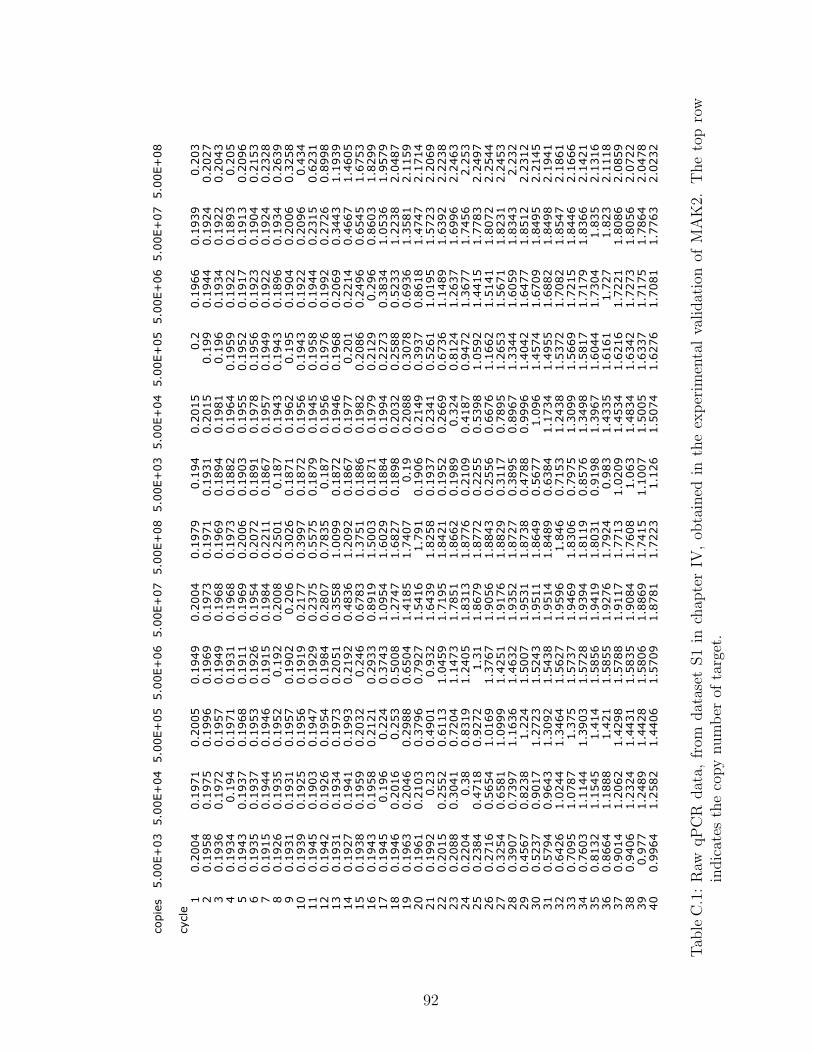
copies5.00E+035.00E+045.00E+055.00E+065.00E+075.00E+085.00E+035.00E+045.00E+055.00E+065.00E+075.00E+08

cycle1

0.2004

0.1971

0.2005

0.1949

0.2004

0.1979

0.194

0.2015

0.2

0.1966

0.1939

0.203

20.1958

0.1975

0.1996

0.1969

0.1973

0.1971

0.1931

0.2015

0.199

0.1944

0.1924

0.2027

30.1936

0.1972

0.1957

0.1949

0.1968

0.1969

0.1894

0.1981

0.196

0.1934

0.1922

0.2043

40.1934

0.194

0.1971

0.1931

0.1968

0.1973

0.1882

0.1964

0.1959

0.1922

0.1893

0.205

50.1943

0.1937

0.1968

0.1911

0.1969

0.2006

0.1903

0.1955

0.1952

0.1917

0.1913

0.2096

60.1935

0.1937

0.1953

0.1926

0.1954

0.2072

0.1891

0.1978

0.1956

0.1923

0.1904

0.2153

70.1915

0.1944

0.1946

0.1915

0.1984

0.2211

0.1867

0.1957

0.1949

0.1922

0.1924

0.2328

80.1926

0.1935

0.1952

0.192

0.2008

0.2501

0.187

0.1943

0.1943

0.1896

0.1934

0.2639

90.1931

0.1931

0.1957

0.1902

0.206

0.3026

0.1871

0.1962

0.195

0.1904

0.2006

0.3258

10

0.1939

0.1925

0.1956

0.1919

0.2177

0.3997

0.1872

0.1956

0.1943

0.1922

0.2096

0.434

11

0.1945

0.1903

0.1947

0.1929

0.2375

0.5575

0.1879

0.1945

0.1958

0.1944

0.2315

0.6231

12

0.1942

0.1926

0.1954

0.1984

0.2807

0.7835

0.187

0.1956

0.1976

0.1992

0.2726

0.8998

13

0.1931

0.1934

0.1973

0.2051

0.3558

1.0099

0.1872

0.1946

0.1968

0.2069

0.3443

1.1939

14

0.1927

0.1941

0.1993

0.2192

0.4836

1.2092

0.1867

0.1977

0.201

0.2214

0.4667

1.4605

15

0.1938

0.1959

0.2032

0.246

0.6783

1.3751

0.1886

0.1982

0.2086

0.2496

0.6545

1.6753

16

0.1943

0.1958

0.2121

0.2933

0.8919

1.5003

0.1871

0.1979

0.2129

0.296

0.8603

1.8299

17

0.1945

0.196

0.224

0.3743

1.0954

1.6029

0.1884

0.1994

0.2273

0.3834

1.0536

1.9579

18

0.1946

0.2016

0.253

0.5008

1.2747

1.6827

0.1898

0.2032

0.2588

0.5233

1.2238

2.0487

19

0.1963

0.2046

0.2988

0.6504

1.4185

1.7407

0.19

0.2088

0.3078

0.6936

1.3581

2.1159

20

0.1961

0.2103

0.3796

0.7927

1.5416

1.791

0.1906

0.2149

0.3937

0.8618

1.4747

2.1714

21

0.1992

0.23

0.4901

0.932

1.6439

1.8258

0.1937

0.2341

0.5261

1.0195

1.5723

2.2069

22

0.2015

0.2552

0.6113

1.0459

1.7195

1.8421

0.1952

0.2669

0.6736

1.1489

1.6392

2.2238

23

0.2088

0.3041

0.7204

1.1473

1.7851

1.8662

0.1989

0.324

0.8124

1.2637

1.6996

2.2463

24

0.2204

0.38

0.8319

1.2405

1.8313

1.8776

0.2109

0.4187

0.9472

1.3677

1.7456

2.253

25

0.2384

0.4718

0.9272

1.31

1.8679

1.8772

0.2255

0.5398

1.0592

1.4415

1.7783

2.2497

26

0.2716

0.5654

1.0169

1.3767

1.9056

1.8843

0.2556

0.6676

1.1662

1.5141

1.8072

2.2544

27

0.3254

0.6581

1.0999

1.4251

1.9176

1.8829

0.3117

0.7895

1.2653

1.5671

1.8231

2.2453

28

0.3907

0.7397

1.1636

1.4632

1.9352

1.8727

0.3895

0.8967

1.3344

1.6059

1.8343

2.232

29

0.4567

0.8238

1.224

1.5007

1.9531

1.8738

0.4788

0.9996

1.4042

1.6477

1.8512

2.2312

30

0.5237

0.9017

1.2723

1.5243

1.9511

1.8649

0.5677

1.096

1.4574

1.6709

1.8495

2.2145

31

0.5794

0.9643

1.3092

1.5438

1.9514

1.8489

0.6384

1.1734

1.4955

1.6882

1.8498

2.1941

32

0.6426

1.0244

1.3464

1.5627

1.9596

1.846

0.7153

1.2438

1.5372

1.7082

1.8547

2.1861

33

0.7095

1.0787

1.375

1.5737

1.9469

1.8306

0.7975

1.3099

1.5669

1.7215

1.8446

2.1666

34

0.7603

1.1144

1.3903

1.5728

1.9394

1.8119

0.8576

1.3498

1.5817

1.7179

1.8366

2.1421

35

0.8132

1.1545

1.414

1.5856

1.9419

1.8031

0.9198

1.3967

1.6044

1.7304

1.835

2.1316

36

0.8664

1.1888

1.421

1.5855

1.9276

1.7924

0.983

1.4335

1.6161

1.727

1.823

2.1118

37

0.9014

1.2062

1.4298

1.5788

1.9117

1.7713

1.0209

1.4534

1.6216

1.7221

1.8086

2.0859

38

0.9406

1.2324

1.4431

1.5835

1.9084

1.7608

1.063

1.4834

1.6342

1.7273

1.8056

2.0722

39

0.977

1.2489

1.4428

1.5806

1.8869

1.7415

1.1007

1.5005

1.6337

1.7175

1.7864

2.0478

40

0.9964

1.2582

1.4406

1.5709

1.8781

1.7223

1.126

1.5074

1.6276

1.7081

1.7763

2.0232

Tab

leC

.1:

Raw

qP

CR

dat

a,fr

omdat

aset

S1

inch

apte

rIV

,ob

tain

edin

the

exp

erim

enta

lva

lidat

ion

ofM

AK

2.T

he

top

row

indic

ates

the

copy

num

ber

ofta

rget

.

92

Data obtained on the MAK2 parameter k

Trends for k seemed to be different for each dataset analyzed. The significance of

the parameter k is not yet understood.

- 10 - 9 - 8 - 7 - 6 - 50.02

0.04

0.06

0.08

0.10

rutledge

- 11 - 10 - 9 - 8 - 7 - 6 - 5 - 40.0

0.5

1.0

1.5

2.0

reps

- 9 - 8 - 7 - 6 - 5 - 4

0.1

0.2

0.3

0.4

Dataset S1

log D0log D0log D0

k

Figure C.2: Dependence of k on D0. The plots show k vs. log(D0), for the threedifferent datasets, following optimization of MAK2 to the data.

93

APPENDIX D

Materials and methods used in experimental

validation of MAK3 fitting to MMQPCR data

Materials and Methods

MMQPCR Assays on synthetic DNA

Two synthetic template DNA sequences (sequences A and B) were designed by

generating random sequences and minimizing secondary structure and off-target primer

binding through editing. The sequences were designed to have a difference in melting

temperature of 2◦C. Secondary structure and off-target primer binding were identified

and their thermodynamic properties were calculated using Visual OMP software from

DNA Software (Ann Arbor, MI). Melting behavior was predicted using the Poland

server for thermal denaturation of nucleic acids (Steger , 1994). Primer and target

DNA were obtained from Integrated DNA Technologies (Coralville, IA).

The target sequence A was:

GACAGGTTTACATGGAACGCCACGAGGATAATCACAATGGCAATCCAGTG-

TATTTGAACGATTATGAAGTGTAGTAACTCGCATTGATCAAGCAAGCCAG-

CCACGAAGGATAGACAGAAACAGGATTCC

94

The sense primer for sequence A was: GGAATCCTGTTTCTGTCTATCC

The antisense primer for sequence A was: GACAGGTTTACATGGAACGC

The target sequence B was:

GTCACGCAGATCTATAGAGTCCAACGAACTAGGTATCGGCGACCATTTGT-

GTGGTACTGGGGACTACGGTGCCGCTAACAACCTCTCGCTGACGTTTGTA-

GTCTAGTCTCATTATGTCGTACAGCTATTCAGAGTGTGACTGATACCGGA-

AGACATCTC

The sense primer for sequence B was: GAGATGTCTTCCGGTATCAGT

The antisense primer for sequence B was: GTCACGCAGATCTATAGAGTCC

Quantitative PCR assays were performed in 25 µL samples on an MJ Research

(BioRad) Chromo4 thermal cycler. Reaction buffer was composed of 0.1 units/µL

HotStart Paq5000 DNA Polymerase (Stratagene, La Jolla, CA) in the supplied reac-

tion buffer, 0.2 mM of each dNTP (Promega, Madison, WI), 2 µM of the dsDNA dye

SYTO-13 (Invitrogen, Carlsbad, CA) and 400 nM of each primer.

The thermal cycling protocol contained a two-minute incubation period at 95.0◦C

followed by forty cycles with a 20s incubation at 95.0◦C and a 60s incubation at

64.0◦C with 4 plate reads obtained at 15s intervals. A melt profile was obtained after

the 11th cycle and for every cycle thereafter (for a total of 30 melt profiles). The

melt profile consisted of plate reads obtained after a 5s incubation at temperatures

ranging from 79.0 to 83.8◦C in 0.2◦C increments, and reads at 84.0, 84.5, and 85.0◦C

obtained after a 10s incubation.

Quantitative PCR assays were performed in both singleplex reactions and MMQPCR

reactions with sequences A and B. The initial template DNA concentrations used in

the qPCR assays ranged from 5*103 to 5*107 copies per well in 10-fold increments of

the higher Tm sequence (B), with the exception of 5*105. Additionally, two samples

of B at unknown concentration were analyzed. The initial template DNA concentra-

tions for sequence A, the lower Tm sequence, ranged from 5*103 to 5*108 copies per

95

well in 10-fold increments. For monoplex assays of sequence A at 5*103 and 5*104

copies per well, contamination due to sequence B dominated the fluorescence signal

(every well contained primers for both targets). Data for sequence A at 5*103 and at

5*104 copies per well were thus not included in data analysis.

Multiplex qPCR assays were performed for mixtures with a difference in target

concentration of 1000-fold or less as shown in Table 5.1. Assays for each condition

were run in duplicate.

MMQPCR Assays on genomic DNA from the microbial consortium

DNA Isolation

1 mL culture samples were centrifuged at 14,000 rpm for 5 minutes. After dis-

carding supernatant, residual liquid was wicked off cell pellets with a kimwipe. A cell

pellet equivalent volume of 425-600 µm acid washed glass beads was added to each

sample. Samples were wetted with buffer AP1 (Qiagen, Germantown, MD, USA)

supplemented 1:100 with RNase (Qiagen) and then pulverized for one minute using

a clean mortar and pestle. Pulverized samples were resuspended in 400 µL buffer

AP1 (Qiagen) and 4 µL of RNase (Qiagen) and then processed with a DNeasy Plant

Kit (Qiagen) as per the manufacturers protocol, using 50 µL buffer AE for the final

elution step.

Primer Design

Primers were designed using Visual OMP software (DNA Software, Ann Arbor,

MI). Primers for the E. coli target were designed to have a melting temperature of

65◦C and primers for the T. reesei target were designed to have a melting temperature

of 70◦C. Primers were confirmed to be specific for their targets through simulation us-

ing Visual OMP. Primers were also scanned against the E. coli and T. reesei genomes

using ThermoBLAST (DNA Software, Ann Arbor, MI) to confirm that no false am-

96

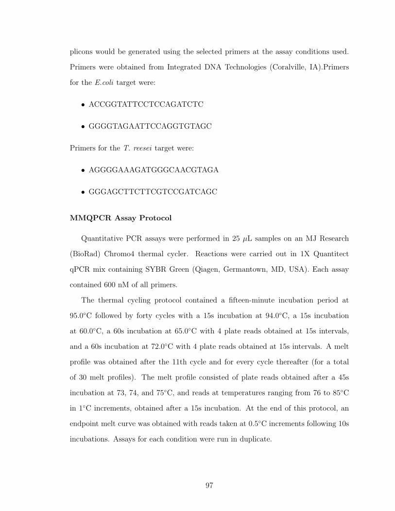
plicons would be generated using the selected primers at the assay conditions used.

Primers were obtained from Integrated DNA Technologies (Coralville, IA).Primers

for the E.coli target were:

• ACCGGTATTCCTCCAGATCTC

• GGGGTAGAATTCCAGGTGTAGC

Primers for the T. reesei target were:

• AGGGGAAAGATGGGCAACGTAGA

• GGGAGCTTCTTCGTCCGATCAGC

MMQPCR Assay Protocol

Quantitative PCR assays were performed in 25 µL samples on an MJ Research

(BioRad) Chromo4 thermal cycler. Reactions were carried out in 1X Quantitect

qPCR mix containing SYBR Green (Qiagen, Germantown, MD, USA). Each assay

contained 600 nM of all primers.

The thermal cycling protocol contained a fifteen-minute incubation period at

95.0◦C followed by forty cycles with a 15s incubation at 94.0◦C, a 15s incubation

at 60.0◦C, a 60s incubation at 65.0◦C with 4 plate reads obtained at 15s intervals,

and a 60s incubation at 72.0◦C with 4 plate reads obtained at 15s intervals. A melt

profile was obtained after the 11th cycle and for every cycle thereafter (for a total

of 30 melt profiles). The melt profile consisted of plate reads obtained after a 45s

incubation at 73, 74, and 75◦C, and reads at temperatures ranging from 76 to 85◦C

in 1◦C increments, obtained after a 15s incubation. At the end of this protocol, an

endpoint melt curve was obtained with reads taken at 0.5◦C increments following 10s

incubations. Assays for each condition were run in duplicate.

97

Data Processing

Real-time melt curves

Real-time melt curves were generated from three-dimensional MMQPCR data by

slicing the data at an individual cycle. The derivative of the intensity with respect

to temperature was calculated as:

dF

dT(T + ∆T ) =

F (T + ∆T )− F (T )

∆T(D.1)

where F(T) is fluorescence intensity at temperature T. The temperature at the trough

between derivative peaks was used as the temperature for measuring signal due to

the high Tm sequence.

qPCR growth curves

qPCR growth curves were generated from three-dimensional MMQPCR data by

slicing the data at an individual temperature. The derivative of the intensity with

respect to cycle was calculated as:

dF

dn(n+ 1) = F (n+ 1)− F (n) (D.2)

where F(n) is fluorescence intensity at cycle n. The cycle with maximum value of

the derivative was used for analyzing the contribution of the high Tm sequence to the

data obtained at low temperature.

MAK3-fitting of MMQPCR Data

MAK3 is a version of the mechanistic model MAK2 that uses an additional pa-

rameter, m in (D.4), to adjust for sloping background in qPCR data. A prototype

version of MAK3 (provided in appendix E) has been developed for use with the qpcR

package for the programming language R (Ritz and Spiess , 2008). The slope ad-

98

justment of MAK3 was necessary for fitting growth curve data obtained at 81.4◦C,

but also results in a better fit for qPCR data in general (AN Spiess, unpublished

observations). The MAK3 model used for fitting data is expressed as:

Dn = Dn−1 + k ln(1 +Dn−1

k) (D.3)

Fn = Dn + (m ∗ n+ Fb) (D.4)

where Dn represents fluorescence due to DNA at cycle n, Fb represents initial back-

ground fluorescence, m represents the slope of background fluorescence, Fn is the

total fluorescence at cycle n, and k is the characteristic PCR constant. The back-

ground fluorescence is thus accounted for by the terms in parentheses in equation

(D.4). Note that when m is 0, the MAK3 model is equivalent to MAK2 (Boggy and

Woolf , 2010). The prototype version of the algorithm used in this study truncated

qPCR data at the cycle where a fitted 4-parameter sigmoid has a maximum value for

the second derivative. An additional two cycles beyond this cutoff were used for data

quantification by setting the correction factor “correct” to a value of 2.

Cq Standard Curve Quantification

The quantification cycle (Cq) is the fractional cycle at which the growth curve

crosses some threshold intensity above background fluorescence.

Cq calculation for low temperature data

The first step involved in calculating Cq for MMQPCR data collected at 64◦C

was to find the value for background fluorescence. This was accomplished by finding

the last cycle where fluorescence is less than the previous cycle. The background

fluorescence was calculated as the average value of fluorescence intensity prior to and

including this cycle. Next, the quantification cycle was calculated by interpolating

99

the fractional cycle at which the growth curve crossed the threshold value above

the background fluorescence. The threshold value used for comparing Cq standard

curve quantification to MAK3 quantification was the value that produced the best

correlation between estimated and known DNA amount.

Cq calculation for high temperature data

Because the background fluorescence sloped upward at 81.4◦C, the procedure for

calculating Cq differed slightly from the procedure used for calculating Cq for data

collected at 64 ◦C. The background fluorescence trend line was determined by find-

ing the best-fit line to the first four datapoints. The quantification cycle was then

calculated by interpolating the fractional cycle at which the growth curve crossed the

threshold value above the background fluorescence trend line. The threshold value

used for comparing Cq standard curve quantification to MAK3 quantification was the

value that produced the best correlation between estimated and known DNA amount.

Data Analysis

Calculation of the ratio of MMQPCR-predicted concentration to monoplex

qPCR-predicted concentration ([Target]multi : [Target]mono)

The ratio of MMQPCR-predicted concentration to monoplex qPCR-predicted con-

centration was calculated by dividing the D0 value obtained by MAK3-fitting of

MMQPCR by the D0 value obtained by MAK3-fitting of monoplex data.

Assessment of Quantification Accuracy

The quantification plots in figure 5.3 depict the accuracy of quantification of the

two target sequences by MAK3 and by Cq standard curve quantification. To gen-

erate these plots, quantification metrics D0 or Cq were first generated as described

above. Next, the best fit linear relationship between log(D0) and log(N0) (where N0

100

is the initial amount of target DNA) or between Cq and log(N0) was found by linear

model-fitting (function LinearModelFit) of data obtained on known concentrations, in

Mathematica. The mean D0 or Cq value for unknowns was used to calculate “known”

concentrations for including this data in the analysis. The trend equation was then

used to calculate an estimated N0 for each known N0. Finally, a linear model is fit to

this data to obtain an R2 value. The plots in figure 5.3 are log-log plots of estimated

vs. known N0.

Comparison of D0 values for E. coli and T. reesei targets

D0 values for the T. reesei target were calculated based on 30 cycles of data col-

lected after the initial 10 cycles of qPCR. In order to compare D0 values calculated for

E. coli and T. reesei targets in figure 5.4b, the D0 values for the T. reesei target were

divided by 210, to account for amplification occurring during the first 10 cycles. This

assumes a perfect doubling at each cycle, however, this is a reasonable assumption

for the initial cycles of PCR.

101

APPENDIX E

Implementation of MAK3 in R

The following code for MAK3 was developed by Andrej-Nikolai Spiess as a result

of a collaborative effort to implement MAK2, and the slope adjusted MAK2 model

MAK3, into the programming language R. It was used for fitting all data from chapter

V.

mechFit <- function(fluo,

method = c("LM", "optim"),

correct = 0)

{

method <- match.arg(method)

FLUO <- fluo[!is.na(fluo)]

### set 0 to small value

FLUO[FLUO == 0] <- 1E-6

### initial parameters

102

# sigmoidal fit for second deriv max point

sigDAT <- cbind(Cycles = 1:length(FLUO), FLUO)

m <- pcrfit(sigDAT, 1, 2, l4)

cpD2 <- efficiency(m, plot = FALSE)$cpD2 + correct

# cut off all cycles beyond...

sigDAT <- sigDAT[1:floor(cpD2), ]

FLUO <- FLUO[1:floor(cpD2)]

# exponential fit for Fb and D0 start estimates

m2 <- pcrfit(sigDAT, 1, 2, expGrowth)

# make grid of start estimates

D0.start <- coef(m2)[1] * 10^(-4:1)

k.start <- seq(0.1, 3, by = 0.3)

Fb.start <- coef(m2)[3]

slope.start <- coef(lm(FLUO[1:5] ~ I(1:5)))[2]

### create grid of initial parameter values

### to optimize over

START <- expand.grid(D0.start, k.start, Fb.start, slope.start)

### objective function definition for MAK2 method

### cost function is residual sum-of-squares

MAK2 <- function(init, y, opt = TRUE) {

d0 <- init[1]

k <- init[2]

Fb <- init[3]

slope <- init[4]

Fn <- vector(mode = "numeric", length = length(y))

103

for (i in 1:length(y)) {

if (i == 1) Fn[i] <- d0 else Fn[i] <- Fn[i-1]

+ k * log(1 + (Fn[i-1]/k))

}

Fn <- Fn + (slope * (1:length(Fn)) + Fb)

if (method == "LM") res <- y - Fn else res <- sum(y - Fn)^2

if (opt) return(res) else return(Fn)

}

### initialize parameter matrix

parMAT <- matrix(nrow = nrow(START), ncol = 5)

colnames(parMAT) <- c("D0", "k", "Fb", "slope", "RSS")

### nonlinear fitting

for (i in 1:nrow(START)) {

PAR <- as.numeric(START[i, ])

if (method == "LM") OUT <- try(nls.lm(PAR, MAK2, y = FLUO,

control = nls.lm.control(maxiter = 10000),

opt = TRUE), silent = TRUE)

else OUT <- try(optim(PAR, MAK2, y = FLUO,

method = "Nelder-Mead", control = list(maxit = 10000),

opt = TRUE), silent = TRUE)

if (inherits(OUT, "try-error")) next

RSS <- if(method == "LM") sum(OUT$fvec^2) else OUT$value

parMAT[i, ] <- c(OUT$par, RSS)

qpcR:::counter(i)

}

104

cat("\n")

### function for best value fit

yFIT <- function(y, D0, k, Fb, slope, opt = FALSE)

MAK2(c(D0, k, Fb, slope), y = y, opt = opt)

### function for R-square

RSQ.mak2 <- function(y, yfit) {

TSS <- sum((y - mean(y))^2)

RSS <- sum((y - yfit)^2)

1 - (RSS/TSS)

}

### function for AIC

AIC.mak2 <- function(y, yfit) {

RESID <- y - yfit

N <- length(RESID)

w <- rep(1, N)

val <- -N * (log(2 * pi) + 1 - log(N) - sum(log(w))

+ log(sum(w * RESID^2)))/2

attr(val, "df") <- 1L + length(OUT$par)

attr(val, "nobs") <- attr(val, "nall") <- N

class(val) <- "logLik"

aic <- AIC(val)

k <- length(OUT$par) + 1

aic + ((2 * k * (k + 1))/(N - k - 1))

105

}

yFITS <- apply(parMAT[, 1:4], 1, function(x)

yFIT(FLUO, x[1], x[2], x[3], x[4], opt = FALSE))

yFITS <- t(yFITS)

RSQS <- apply(yFITS, 1, function(x) RSQ.mak2(FLUO, x))

AICS <- apply(yFITS, 1, function(x) AIC.mak2(FLUO, x))

parMAT <- cbind.na(parMAT, Rsq = RSQS, AIC = AICS)

ORDER <- order(parMAT[, 5])

parMAT <- parMAT[ORDER, ]

yFITS <- yFITS[ORDER, ]

plot(1:length(fluo), fluo, main =

paste("Rsq:", round(RSQ.mak2(FLUO, yFITS[1, ]), 5)))

lines(yFITS[1, ], col = 2, lwd = 2)

OUT <- parMAT[1, 1]

#OUT <- yFITS[1, ] - parMAT[1, 3]

### return parameters

return(OUT)

}

106

##########

library(qpcR)

### unmark here for testing the different datasets!

DATA <- reps[, 1:25]; GL <- gl(6, 4)

#DATA <- rutledge ; GL <- gl(6, 20)

#DATA <- boggy ; GL <- gl(6, 2)

#DATA <- guescini1 ; GL <- gl(7, 12)

#DATA <- batsch1 ; GL <- gl(5, 3)

#DATA <- sisti1 ; GL <- gl(6, 12)

DATA <- DATA[, -1, drop = F]

## do fitting on datasets

res <- apply(DATA, 2, function(x)

mechFit(x, method = "LM", correct = 0))

LM <- lm(log10(res) ~ rev(as.numeric(GL)))

summary(LM)

stripchart(log10(res) ~ rev(GL), main =

paste("R^2:", round(Rsq(LM), 5)), vertical = TRUE, pch = 16)

abline(LM, col = "red", lwd = 2)

107

BIBLIOGRAPHY

108

A. Spiess, C. R., C. Feig (2008), Highly accurate sigmoidal fitting of real-time PCRdata by introducing a parameter for asymmetry, BMC Bioinformatics, 9.

Altman, D. G., and J. M. Bland (1983), Measurement in medicine - the analysis ofmethod comparison studies, STATISTICIAN, 32 (3), 307–317.

Boggy, G. J., and P. J. Woolf (2010), A mechanistic model of PCR for accu-rate quantification of quantitative PCR data, PLoS ONE, 5 (8), e12,355, doi:10.1371/journal.pone.0012355.

Boggy, G. J., J. Minty, M. E. Singer, A.-N. Spiess, N. Lin, and P. J. Woolf (2011), Sim-plified measurement of multiple DNA targets with monochrome multiplex qPCRand mechanistic data analysis, PLoS ONE, (under review).

Booth, C. S., E. Pienaar, J. R. Termaat, S. E. Whitney, T. M. Louw, and H. J.Viljoen (2010), Efficiency of the polymerase chain reaction, Chemical EngineeringScience, 65 (17), 4996–5006, doi:10.1016/j.ces.2010.05.046.

Borer, P. N., B. Dengler, I. Tinoco, and O. C. Uhlenbec (1974), Stability ofribonucleic-acid double-stranded helices, Journal of Molecular Biology, 86 (4), 843–853.

Cawthon, R. M. (2009), Telomere length measurement by a novel monochrome mul-tiplex quantitative PCR method, Nucleic Acids Research, 37 (3), e21.

Cikos, S., and J. Koppel (2009), Transformation of real-time PCR fluorescence datato target gene quantity, Analytical Biochemistry, 384 (1), 1–10.

Crothers, D. M., and B. H. Zimm (1964), Theory of melting transition of syntheticpolynucleotides - evaluation of stacking free energy, Journal of Molecular Biology,9 (1), 1–.

Devoe, H., and I. Tinoco (1962), Stability of helical polynucleotides - base contribu-tions, Journal of Molecular Biology, 4 (5), 500–.

Edelman, L. B., G. Toia, D. Geman, W. Zhang, and N. D. Price (2009), Two-transcript gene expression classifiers in the diagnosis and prognosis of human dis-eases, BMC Genomics, 10, 583, doi:10.1186/1471-2164-10-583.

Fujimori, M., et al. (2010), Efficacy of bacterial ribosomal RNA-targeted reversetranscription-quantitative PCR for detecting neonatal sepsis: a case control study,BMC Pediatrics, 10, 53, doi:10.1186/1471-2431-10-53.

Gevertz, J. L., S. M. Dunn, and C. M. Roth (2005), Mathematical model of real-timePCR kinetics, Biotechnology and Bioengineering, 92 (3), 346–355.

Gray, D. M., and I. Tinoco (1970), A new approach to study of sequence-dependentproperties of polynucleotides, Biopolymers, 9 (2), 223–.

109

Griep, M., S. Whitney, M. Nelson, and H. Viljoen (2006a), DNA polymerase chainreaction: A model of error frequencies and extension rates, AICHE Journal, 52 (1),384–392, doi:10.1002/aic.10604.

Griep, M. A., C. A. Kotera, R. M. Nelson, and H. J. Viljoen (2006b), Kinetics of theDNA polymerase pyrococcus kodakaraensis, Chemical Engineering Science, 61 (12),3885–3892, doi:10.1016/j.ces.2005.12.032.

Hartshorn, C., J. J. Eckert, O. Hartung, and L. J. Wangh (2007), Single-cell duplexRT-LATE-PCR reveals Oct4 and Xist RNA gradients in 8-cell embryos, BMCBiotechnology, 7, 87, doi:10.1186/1472-6750-7-87.

Heid, C. A., J. Stevens, K. J. Livak, and P. M. Williams (1996), Real Time Quanti-tative PCR, Genome Research, 6 (10), 986–994.

Higuchi, R., C. Fockler, G. Dollinger, and R. Watson (1993), Kinetic PCR Analy-sis: Real-time Monitoring of DNA Amplification Reactions, Bio-Technology, 11 (9),1026–1030.

Kainz, P., A. Schmiedlechner, and H. B. Strack (2000), Specificity-enhanced hot-start PCR: Addition of double-stranded DNA fragments adapted to the annealingtemperature, Biotechniques, 28 (2), 278–282.

Kanagawa, T. (2003), Bias and artifacts in multitemplate polymerase chain reactions(PCR), Journal of Bioscience and Bioengineering, 96 (4), 317–323.

Lee, J. Y., H. W. Lim, S. I. Yoo, B. T. Zhang, and T. H. Park (2006), Simulationand real-time monitoring of polymerase chain reaction for its higher efficiency.

Liu, W. H., and D. A. Saint (2002a), Validation of a quantitative method for real timePCR kinetics, Biochemical and Biophysical Research Communications, 294 (2),347–353.

Liu, W. H., and D. A. Saint (2002b), A new quantitative method of real time reversetranscription polymerase chain reaction assay based on simulation of polymerasechain reaction kinetics, Analytical Biochemistry, 302 (1), 52–59.

Markoulatos, P., N. Siafakas, and M. Moncany (2002), Multiplex polymerase chainreaction: A practical approach, Journal of Clinical Laboratory Analysis, 16 (1),47–51.

Mehra, S., and W. S. Hu (2005), A kinetic model of quantitative real-time polymerasechain reaction, Biotechnology and Bioengineering, 91 (7), 848–860.

Michaelis, L., and M. L. Menten (1913), The kenetics of the inversion effect., Bio-chemische Zeitschrift, 49, 333–369.

Mourah, S., et al. (2009), Quantification of VEGF isoforms and VEGFR transcriptsby qRT-PCR and their significance in acute myeloid leukemia, International Jour-nal of Biological Markers, 24 (1), 22–31.

110

Ninio, J. (1987), Alternative to the steady-state method - derivation of reaction-rates from 1st-passage times and pathway probabilities, Proceedings of the NationalAcademy of Sciences of the United States of America, 84 (3), 663–667.

Pfaffl, M. W. (2001), A new mathematical model for relative quantification in real-time RT-PCR, Nucleic Acids Research, 29 (9), e45.

Pienaar, E., A. Theron, A. Nelson, and H. J. Viljoen (2006), A quantitative model oferror accumulation during PCR amplification, Computational Biology and Chem-istry, 30 (2), 102–111.

Pierce, K. E., J. E. Rice, J. A. Sanchez, and L. J. Wangh (2003), Detection of cysticfibrosis alleles from single cells using molecular beacons and a novel method ofasymmetric real-time PCR, Molecular Human Reproduction, 9 (12), 815–820.

Rasmussen, R. (2001), Quantification on the LightCycler. In Meuer,S., Wittwer,C.and Nakagawara,K. (eds), pp. 21–34, Rapid Cycle Real-time PCR, Methods andApplications., Springer Press, Heidelberg.

Ritz, C., and A. N. Spiess (2008), qpcR: an R package for sigmoidal model selection inquantitative real-time polymerase chain reaction analysis, Bioinformatics, 24 (13),1549–1551.

Rutledge, R. G. (2004), Sigmoidal curve-fitting redefines quantitative real-time PCRwith the prospective of developing automated high-throughput applications, Nu-cleic Acids Research, 32 (22), e178.

Rutledge, R. G., and C. Cote (2003), Mathematics of quantitative kinetic PCR andthe application of standard curves, Nucleic Acids Research, 31 (16), e93.

Rutledge, R. G., and D. Stewart (2008a), A kinetic-based sigmoidal model for thepolymerase chain reaction and its application to high-capacity absolute quantitativereal-time PCR, BMC Biotechnology, 8, 47.

Rutledge, R. G., and D. Stewart (2008b), Critical evaluation of methods used todetermine amplification efficiency refutes the exponential character of real-timePCR, BMC Molecular Biology, 9, 96.

Sanchez, J. A., K. E. Pierce, J. E. Rice, and L. J. Wangh (2004), Linear-After-The-Exponential (LATE)-PCR: An advanced method of asymmetric PCR and its usesin quantitative real-time analysis, Proceedings of the National Academy of Sciencesof the United States of America, 101 (7), 1933–1938.

SantaLucia, J. (1998), A unified view of polymer, dumbbell, and oligonucleotide DNAnearest-neighbor thermodynamics, Proceedings of the National Academy of Sciencesof the United States of America, 95 (4), 1460–1465.

111

SantaLucia, J. (2007), Physical Principles and Visual-OMP Software for OptimalPCR Design, Methods In Molecular Biology, vol. 402, chap. 1, pp. 3–33, HumanaPress, Totowa, NJ.

SantaLucia, J., and D. Hicks (2004), The thermodynamics of DNA structural motifs,Annual Review of Biophysics and Biomolecular Structure, 33, 415–440.

Sizmann, D., et al. (2010), Improved HIV-1 RNA quantitation by COBAS (R) Am-pliPrep/COBAS (R) TaqMan (R) HIV-1 Test, v2.0 using a novel dual-target ap-proach, Journal of Clinical Virology, 49 (1), 41–46, doi:10.1016/j.jcv.2010.06.004.

Smith, C. J., and A. M. Osborn (2009), Advantages and limitations of quantitativePCR (Q-PCR)-based approaches in microbial ecology, FEMS Microbiology Ecology,67 (1), 6–20, doi:10.1111/j.1574-6941.2008.00629.x.

Smith, M. V., C. R. Miller, M. Kohn, N. J. Walker, and C. J. Portier (2007), Absoluteestimation of initial concentrations of amplicon in a real-time RT-PCR process,BMC Bioinformatics, 8, 409.

Steger, G. (1994), Thermal-denaturation of double-stranded nucleic-acids - predic-tion of temperatures critical for gradient gel-electrophoresis and polymerase chain-reaction, Nucleic Acids Research, 22 (14), 2760–2768.

Swillens, S., B. Dessars, and H. El Housni (2008), Revisiting the sigmoidal curvefitting applied to quantitative real-time PCR data, Analytical Biochemistry, 373 (2),370–376.

Tichopad, A., M. Dilger, G. Schwarz, and M. W. Pfaffl (2003), Standardized deter-mination of real-time PCR efficiency from a single reaction set-up, Nucleic AcidsResearch, 31 (20), e122.

Tinoco, I., P. N. Borer, B. Dengler, M. D. Levine, O. C. Uhlenbec, D. M. Crothers,and J. Gralla (1973), Improved estimation of secondary structure in ribonucleic-acids, Nature-New Biology, 246 (150), 40–41.

Tyagi, S., and F. R. Kramer (1996), Molecular beacons: Probes that fluoresce uponhybridization, Nature Biotechnology, 14 (3), 303–308.

Uhlenbec, O. C., P. N. Borer, B. Dengler, and I. Tinoco (1973), Stability of RNAhairpin loops, Journal of Molecular Biology, 73 (4), 483–496.

Van Slyke, D. D., and G. E. Cullen (1914), The mode of action of urease and ofenzymes in general., Journal of Biological Chemistry, 19 (2), 141–180.

VanGuilder, H. D., K. E. Vrana, and W. M. Freeman (2008), Twenty-five years ofquantitative PCR for gene expression analysis, Biotechniques, 44 (5), 619–626, doi:10.2144/000112776.

112

Viljoen, S., M. A. Griep, M. Nelson, and H. Viljoen (2005), A macro-scopic kinetic model for DNA polymerase elongation and high-fidelity nu-cleotide selection, Computational Biology and Chemistry, 29 (2), 101–110, doi:10.1016/j.compbiolchem.2005.02.003.

Whitcombe, D., J. Theaker, S. P. Guy, T. Brown, and S. Little (1999), Detection ofPCR products using self-probing amplicons and fluorescence, Nature Biotechnology,17 (8), 804–807.

113