engineering recommendation erec s34 issue 2 2017 a guide ... · ena engineering recommendation erec...
TRANSCRIPT

PRODUCED BY THE OPERATIONS DIRECTORATE OF ENERGY NETWORKS ASSOCIATION
www.energynetworks.org
Engineering Recommendation EREC S34 Issue 2 2017
A GUIDE FOR ASSESSING THE RISE OF EARTH POTENTIAL AT ELECTRICAL INSTALLATIONS

PUBLISHING AND COPYRIGHT INFORMATION
First published 1986.
Amendments since publication
Issue Date Amendment
1 May 1986 Amendment 1 – Minor changes to figure 17
1 1988 Amendment 2 – Minor changes to formulae on pages 25 and 27
2 October 2017
Major revision and re-write. Alignment with latest revisions of BS EN 50522, BS 7430 and ENA TS 41-24. New formulae introduced.
© 2017 Energy Networks Association
All rights reserved. No part of this publication may be reproduced, stored in a retrieval system or transmitted in any form or by any means, electronic, mechanical, photocopying, recording or otherwise, without the prior written consent of Energy Networks Association. Specific enquiries concerning this document should be addressed to:
Operations Directorate Energy Networks Association 6th Floor, Dean Bradley House
52 Horseferry Rd London
SW1P 2AF
This document has been prepared for use by members of the Energy Networks Association to take account of the conditions which apply to them. Advice should be taken from an appropriately qualified engineer on the suitability of this document for any other purpose.

ENA Engineering Recommendation EREC S34 Issue 2 October 2017
Page 3
Contents
Introduction ............................................................................................................................... 81 Scope ................................................................................................................................. 82 Normative references ......................................................................................................... 83 Terms and definitions ......................................................................................................... 8
3.1 Symbols used ........................................................................................................... 83.2 Formulae used for calculating earth installation resistance for earthing studies ...... 83.3 Description of system response during earth fault conditions .................................. 9
4 Earth fault current studies ................................................................................................ 114.1 Earth fault current ................................................................................................... 114.2 Fault current analysis for multiple earthed systems ................................................ 114.3 Induced currents in parallel conductors .................................................................. 12
4.3.1 Simple circuit representation for initial estimates ....................................... 124.3.2 More realistic circuit representation to improve the accuracy of
calculations ................................................................................................. 124.3.3 Amending calculations to account for increased ground return current
in single-core circuits that are not in trefoil touching arrangement ............. 135 EPR impact calculations ................................................................................................... 14
5.1 Calculation of touch potentials ................................................................................ 145.2 Calculation of step potentials .................................................................................. 145.3 Surface potential contours ...................................................................................... 145.4 Transfer potential to LV systems where the HV and LV earthing are separate ...... 14
5.4.1 Background ................................................................................................ 145.4.2 Basic theory ................................................................................................ 15
5.5 Methods of optimising the design ........................................................................... 175.5.1 More accurate evaluation of fault current ................................................... 175.5.2 Reducing the overall earth impedance ....................................................... 175.5.3 Reducing the touch potential within the installation .................................... 17
5.6 Risk assessment methodology ............................................................................... 176 Case study examples ....................................................................................................... 18
6.1 Case study 1: 33 kV substation supplied via overhead line circuit ......................... 186.1.1 Resistance calculations .............................................................................. 196.1.2 Calculation of fault current and earth potential rise .................................... 256.1.3 Calculation of touch potentials .................................................................... 256.1.4 External touch potential at the edge of the electrode ................................. 266.1.5 Touch potential on fence ............................................................................ 276.1.6 Internal touch potentials ............................................................................. 276.1.7 Calculation of external voltage impact contours ......................................... 27
6.2 Case study 2: 33 kV substation supplied via cable circuit ...................................... 286.2.1 Resistance calculations .............................................................................. 286.2.2 Calculation of fault current and EPR ............................................................ 296.2.3 C-factor method .......................................................................................... 29

ENA Engineering Recommendation EREC S34 Issue 2 October 2017 Page 4
6.2.4 Matrix method ............................................................................................. 306.2.5 Results ........................................................................................................ 31
6.3 Case study 3: 33 kV substation supplied via mixed overhead line/cable circuit ..... 316.3.1 Resistance calculations .............................................................................. 326.3.2 Calculation of fault current and earth potential rise .................................... 32
6.4 Case study 4: Multiple neutrals ............................................................................... 346.4.1 Introduction ................................................................................................. 346.4.2 Case study data .......................................................................................... 366.4.3 Treatment of neutral current ....................................................................... 366.4.4 Fault current distribution ............................................................................. 376.4.5 Earth potential rise (EPR) ............................................................................ 38
6.5 Case study 5: 11 kV substation and LV earthing interface ..................................... 386.5.1 Design option 1 ........................................................................................... 386.5.2 C-factor method .......................................................................................... 396.5.3 Matrix method ............................................................................................. 406.5.4 Results ........................................................................................................ 406.5.5 Surface current density ............................................................................... 406.5.6 Design option 2 ........................................................................................... 416.5.7 C-factor method .......................................................................................... 426.5.8 Matrix method ............................................................................................. 426.5.9 Results ........................................................................................................ 43
APPENDICES ........................................................................................................................ 44Appendix A Symbols used within formulae or figures .................................................... 45Appendix B Formulae .................................................................................................... 48Appendix C Earthing design methodology ..................................................................... 58Appendix D Formulae for determination of ground return current for earth faults
on metal sheathed cables ................................................................................................ 59Appendix E Ground current for earth faults on steel tower supported circuits with
an aerial earth wire .......................................................................................................... 69Appendix F Typical values of resistance of long horizontal electrode ........................... 70Appendix G Chain impedance of standard 132kV earthed tower lines .......................... 71Appendix H The effect on ground return current for changes in geometry .................... 72Appendix I Transfer potential to distributed LV systems .............................................. 77Bibliography ............................................................................................................................ 81
ENA Engineering Recommendation EREC S34 Issue 2 October 2017
Page 5
Figures
Figure 1 — Earth fault at an installation which has an earthed tower line supply .................. 10Figure 2 — Equivalent circuit for analysis .............................................................................. 11Figure 3 — Surface potential near a simple HV and LV electrode arrangement ................... 16Figure 4 — Equivalent circuit for combined LV electrodes A and B ....................................... 16Figure 5 — Case study 1: Supply arrangement ..................................................................... 19Figure 6 — Substation B basic earth grid ............................................................................... 20Figure 7 — Substation B basic earth grid and rods ................................................................ 21Figure 8 — Substation B earth grid with rods and re-bar ....................................................... 23Figure 9 — Case study 2: Supply arrangement ..................................................................... 28Figure 10 — Case study 3: Supply arrangement ................................................................... 31Figure 11 — Case study 3: Equivalent circuit ........................................................................ 32Figure 12 — Case study 4: Supply arrangement ................................................................... 36Figure 13 — Case study 5: Option 1 ...................................................................................... 38Figure 14 — Case study 5: Option 2 ...................................................................................... 41Figure B.1 — factor k for formula R5 ...................................................................................... 49Figure D.1 — Cable circuit, local source, fault at cable end ................................................... 59Figure D.2 — Cable-line circuit, local source, remote fault .................................................... 60Figure D.3 — Line-cable circuit, remote source, fault at cable end ........................................ 61Figure D.4 — Line-cable-line circuit, remote source, remote fault ......................................... 62Figure F.1 — Typical values of resistance of long horizontal electrode (taken from BS EN 50522) .............................................................................................................................. 70Figure H.1 — Cross-sectional view for cable 3 ...................................................................... 73Figure H.2 — Circuit used for analysis purposes ................................................................... 73Figure H.3 — Ground return current (IE) as a percentage of (IF) against circuit length for different 132 kV cable installation arrangements .............................................................. 74Figure H.4 — Ground return current (IE) as a percentage of (IF) against circuit length for different 11 kV cable installation arrangements ................................................................ 75Figure I.1 — Example 1: Two electrodes of equal resistance ................................................ 77Figure I.2 — Example 2: Two electrodes of unequal resistance ............................................ 78Figure I.3 — Example of pole-mounted 11 kV substation arrangement and LV supply to a dwelling ........................................................................................................................... 80

ENA Engineering Recommendation EREC S34 Issue 2 October 2017 Page 6
Tables
Table 1 — Fault clearance time and permissible touch potentials ......................................... 19Table 2 — EPR for different grid arrangements ...................................................................... 25Table 3 — Fault clearance time and permissible touch potentials ......................................... 28Table 4 — Input data and results ........................................................................................... 29Table 5 — Complex representation of cable self and mutual impedances ............................ 30Table 6 — Resultant fault current distribution and EPR(matrix method) ................................ 31Table 7 — Input data and results for final part of circuit ......................................................... 33Table 8 — Input data and results for initial part of circuit ....................................................... 34Table 9 — Case study 4: Short-circuit data ............................................................................ 36Table 10 — Sum of contributions to earth fault current .......................................................... 36Table 11 — Information for fault current distribution calculations .......................................... 37Table 12 — Calculated ground return current ........................................................................ 37Table 13 —Option 1 input data and results ............................................................................ 40Table 14 — Resultant fault current distribution and EPR (matrix method) .............................. 40Table 15 — Option 2 input data and results ........................................................................... 42Table 16 — Resultant fault current distribution and EPR (matrix method) .............................. 42Table B.1 - Approximate lengths for a single horizontal earth wire, tape or PILCSWA cable beyond which no further significant reduction in resistance can be obtained ............... 50Table D.1 — Self and mutual impedances for a sample of three-core cables ....................... 65Table D.2 — Self and mutual impedances for a sample of single-core (triplex) cables ......... 66Table E.1 — Ground return current as % of earth fault current for tower lines ...................... 69Table G.1 — Chain impedance for 132 kV tower lines .......................................................... 71Table H.1 — Technical details of cables modelled ................................................................ 72Table H.2 — Geometric placement of cables ......................................................................... 72

ENA Engineering Recommendation EREC S34 Issue 2 October 2017
Page 7
Foreword 1
This Engineering Recommendation (EREC) is published by the Energy Networks Association 2 (ENA) and comes into effect from xxxx, 2017. It has been prepared under the authority of the 3 ENA Engineering Policy and Standards Manager and has been approved for publication by the 4 ENA Electricity Networks and Futures Group (ENFG). The approved abbreviated title of this 5 engineering document is “EREC S34”, which replaces the previously used abbreviation “ER 6 EREC S34”. 7

ENA Engineering Recommendation EREC S34 Issue 2 October 2017 Page 8
Introduction 8
This Engineering Recommendation (EREC) is the technical supplement to ENA TS 41-24 9 (2017), providing formulae, guidelines and examples of the calculations necessary to estimate 10 the technical parameters associated with earth potential rise (EPR). 11
ENA TS 41-24 provides the overall rules, the design process, safety limit values and links with 12 legislation and other standards. 13
1 Scope 14
This document describes the basic design calculations and methods used to analyse the 15 performance of an earthing system and estimate the earth potential rise created, for the range 16 of electrical installations within the electricity supply system in the United Kingdom covered by 17 ENA TS 41-24. Modification to the calculations and methods may be necessary before they can 18 be applied to rail, industrial and other systems. 19
2 Normative references 20
The following referenced documents, in whole or part, are indispensable for the application of 21 this document. For dated references, only the edition cited applies. For undated references, the 22 latest edition of the referenced document (including any amendments) applies. 23
ENA TS 41-24 also contains an extensive list of reference documents. 24
Standards publications 25
BS EN 50522:2011, Earthing of power installations exceeding 1 kV a.c. 26
ENA TS 41-24, Guidelines for the Design, Installation, Testing and Maintenance of Main 27 Earthing Systems in Substations 28
BS EN 60909-3:2010, Short-circuit currents in three-phase a.c. systems. Currents during two 29 separate simultaneous line-to-earth short-circuits and partial short-circuit currents flowing 30 through earth 31
3 Terms and definitions 32
3.1 Symbols used 33 Symbols or a similar naming convention to BS EN 50522 have been used throughout and are 34 listed in Appendix A. Where these differ from the symbols used in earlier versions of this 35 document, the previous symbols are shown alongside the new ones, to assist when checking 36 previous calculations. 37
3.2 Formulae used for calculating earth installation resistance for earthing studies 38 The most common formulae for power installations are given in Appendix B. These are 39 generally used to calculate the resistance of an earth electrode system comprising of horizontal 40 and/or vertical components or voltages at points of interest. 41
NOTE 1: Formulae in this document are those which are considered most relevant to UK network operators. They 42 may differ from those in BS EN 50522 where the BS EN version is known to be a simplification and/or restricted in its 43 application. 44 NOTE 2: Unless reference to another part of this document is given, all references to formulae, e.g. P1, R1, refer to 45 those in Appendix B. 46

ENA Engineering Recommendation EREC S34 Issue 2 October 2017
Page 9
NOTE 3: Some formulae taken from other standards have definitions that may not be consistent with the main body 47 of this document – e.g. formula P4 has alternative definitions for some of the parameters. These have been retained 48 to avoid the need for alternative definitions and to allow easy cross reference with source material. 49 When using formulae to calculate earth resistances, caution is necessary because they do not 50 normally account for proximity effects or the longitudinal impedance of conductors. 51
For first estimates, the overall impedance 𝑍% of separate electrodes with respect to reference 52 earth is taken as the sum of their separate values in parallel. For the example shown in Figure 53 1 this would be: 54
𝑍% =1𝑅%)
+1
𝑍+,-+
1𝑍+,.
+ ⋯0-
55
In reality, 𝑍% will be higher if the separate electrodes are close enough that there is significant 56 interaction between them (proximity effect). Proximity effects can be accounted for in most 57 advanced software packages. When relying on standard formulae, the following techniques can 58 help to account for proximity when calculating𝑍%: 59
• Include any radial electrodes that are short in relation to the substation size, into the overall 60 calculation of the earth grid resistance. 61
• For radial spur electrodes or cables with an electrode effect, assume the first part of its 62 length is insulated over a distance similar to the substation equivalent diameter. Calculate 63 the earth resistance of the remainder of the electrode/cable and add the longitudinal 64 impedance of the insulated part in series. 65
• For a tower line, assume that the line starts after one span of overhead earth wire (the 66 longitudinal impedance of this earth wire/span would be placed in series with the tower line 67 chain impedance). 68
A value of soil resistivity is needed and for the formulae in Appendix B, this should be a uniform 69 equivalent (see ENA TS 41-24, Section 7.4.) For soils that are clearly of a multi-layer structure 70 with significant resistivity variations between layers, the formulae should be used with caution 71 and it is generally better to use dedicated software that accounts for this to provide results of the 72 required level of accuracy. 73
3.3 Description of system response during earth fault conditions 74 The arrangement shown in Figure 1 is based upon the example described in BS EN 50522 and 75 will be explained and developed further in this document. The EPR is the product of earth 76 electrode impedance and the current that flows through it into the soil and back to its remote 77 source. The description below demonstrates how the fault current and associated impedances 78 are used to arrive at the components that are relevant to the EPR. 79
The installation is based on a ground-mounted substation that is supplied from (or looped into) 80 an overhead line circuit that is supported on steel towers and has an over-running earth wire. In 81 this simplified example, currents are shown only on one of the infeed circuits for clarity, and flow 82 in one earth wire only. It is also assumed that each tower line supports only one (three-phase) 83 circuit. 84
The fault condition is a high voltage phase insulation failure to earth within the substation. It is 85 possible to model this situation with computer software such that all of the effects are summated, 86 calculated and results presented together. For traditional analysis in this standard, the effects 87 are decoupled as described below. 88
89

ENA Engineering Recommendation EREC S34 Issue 2 October 2017 Page 10
90
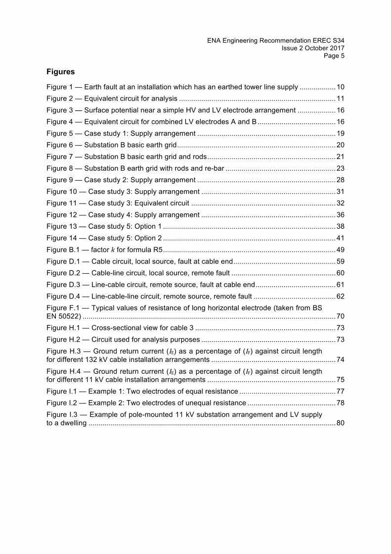
Figure 1 — Earth fault at an installation which has an earthed tower line supply 91
The total earth fault current at the point of fault (𝐼3 ) that will flow into the earth grid and 92 associated components would be reduced initially by two components. 93
• The first component is that passing through the transformer star point earth connection (𝐼4) 94 and returning to source via the unfaulted phase conductors. For systems that are normally 95 multiply earthed, i.e. at 132 kV and above, the total current excluding the 𝐼4 component is 96 normally calculated by summating the currents in all three phases (3𝐼5) vectorially. The 97 process is further described in case study 4 (Section 6.4). For lower voltage distribution 98 systems, 𝐼4is normally zero or sufficiently low to be ignored in calculations. 99
• The second reduction is due to inductive coupling between the faulted phase and 100 continuous earth conductor (see Section 4.3). This part of the current is normally pre-101 calculated for standard line arrangements or can be individually calculated from the support 102 structure geometry, conductor cross section and material. A similar procedure is followed for 103 a buried cable. Another approach is to use a reduction factor rE based on the specific circuit 104 geometry and material. 105
Once these components have been removed, the situation is shown in Figure 2. The earth 106 current (𝐼%) is treated as flowing into the earth network, which in this example contains the 107 substation earth grid (resistance𝑅%)) and two ‘chain impedances’ of value 𝑍+,- and𝑍+,.. The 108 two chain impedances are each a ladder network consisting of the individual tower footing 109 resistance 𝑅%7 in series with the longitudinal impedance of each span of earth wire. They are 110 treated as being equal if they have more than 20 similar towers in series and are in soil of 111 similar resistivity. The overall impedance of the electrode network is 𝑍% and the current (𝐼%) 112 flowing through it creates the earth potential rise (𝑈%). 113
The analysis of the performance of the system described follows the process shown in the 114 design methodology flow diagram (Appendix C). The case studies in Section 6 illustrate this 115 process for a number of examples of increasing complexity. 116
ENA Engineering Recommendation EREC S34 Issue 2 October 2017
Page 11
117
118 Figure 2 — Equivalent circuit for analysis 119
120
4 Earth fault current studies 121
This section describes how to use the fault current data (calculated using the methodology set 122 out in BS EN 60909 and guidance from ENA TS 41-24, Section 5.4) for earth potential rise 123 purposes. 124
4.1 Earth fault current 125 Source earth fault current values (such as the upper limit with neutral earth resistors in place) 126 may be used for initial feasibility studies, but for design purposes, the value used should be site 127 specific, i.e. should account for the fault resistance and longitudinal phase impedance between 128 the source and installation. 129
Once the fault current is known, the clearance time for a normal protection operation (as defined 130 in ENA TS 41-24), at this level of current should be determined and the applicable safety 131 voltage limits obtained from ENA TS 41-24, Tables 1 and 2. This basis of a normal protection 132 operation is used for the personnel protection assessment. Design measures should be 133 included within installations to afford a higher level of protection to personnel in the event of a 134 main protection failure. 135
For protection and telecommunication equipment immunity studies in distribution systems, the 136 steady state RMS fault current values are normally used. At some installations, particularly 137 where there are significant generation in-feeds, consideration should be given to sub-transient 138 analysis. This is especially important where vulnerable equipment (such as a telephone 139 exchange) is installed close to a generation installation. 140
For calculation of the EPR, it is the ground return component of the fault current (𝐼%) that is of 141 concern. On some transmission systems, this can be greater for a phase-phase-earth fault 142 (compared to a straightforward phase-earth fault) and where applicable, this value should be 143 used for the EPR calculation. 144
4.2 Fault current analysis for multiple earthed systems 145 The methodology followed in this document assumes that the earth fault current at the 146 substation (possibly at a defined point in the substation) has been separately calculated using 147 power system analysis tools, symmetrical components or equivalent methods. Depending upon 148

ENA Engineering Recommendation EREC S34 Issue 2 October 2017 Page 12
the complexity of the study, the data required may be a single current magnitude or the three 149 phase currents in all supply circuits in vector format. 150
4.3 Induced currents in parallel conductors 151 The alternating current that flows in a conductor (normally a phase conductor) will create a 152 longitudinal emf in conductors that lie in parallel with it. These are typically cable metal screens 153 (lead sheath, steel armour or copper strands), earth wires laid with the circuit, metal pipes, 154 traction rails or the earth wires installed on overhead lines. This emf will increase from the point 155 of its earth connection as a function of the length of the parallelism and other factors (such as 156 the separation distance). If the remote end of the parallel conductor is also connected to earth, 157 then a current will circulate through it, in the opposite general direction to the inducing current. 158
The current that flows (returns) via the cable sheath or earth wire during fault conditions can be 159 large and it has the effect of reducing the amount of current flowing into the ground via the 160 electrode system, resulting in a reduced EPR on it. 161
The following sections provide methods to account for these return currents. 162
4.3.1 Simple circuit representation for initial estimates 163 For an overhead line with a single earth wire, or a single cable core and its earth sheath, the 164 formulae below approximate the ground return current (𝐼%). The main assumption is that the 165 circuit is long enough such that the combined value of the earthing resistances at each end of 166 the line are small compared with 𝑧: (earth wire impedance), or for cable, small compared with 𝑟< 167 (cable sheath resistance). 168
For an overhead line (refer to Figure 1): 169
𝐼% = 𝑘 𝐼3 − 𝐼4 where𝑘 = 1 −𝑧?@,:𝑧:
170
where 𝑧?@,: is the mutual impedance between the line conductors and earth wire. 171
NOTE: All terms are vector quantities 172 Appendix E gives calculated values of 𝐼% presented as a percentage of overall earth-fault 173 current 𝐼3, and phase angle with respect to 𝐼3 for a range of the most commonly used overhead 174 line constructions at 132 kV, 275 kV and 400 kV. 175
For a single-core cable: 176
𝐼% = 𝑘 𝐼3 − 𝐼4 where𝑘 =𝑟<𝑧<
177
181 NOTE: The formulae are not sufficiently accurate for circuits less than 1 km in length. The results are also sensitive to 178 low values of terminal (electrode) resistance. In these cases, the more detailed approach presented in Section 4.3.2 179 will be required. 180 4.3.2 More realistic circuit representation to improve the accuracy of calculations 182 More complete formulae are given in Appendix D. They require a number of circuit factors and 183 cable-specific C-factors to provide sufficiently accurate results. C-factors have been included in 184 Tables D.1 and D.2 for a representative sample of cables. 185
The case studies have been selected to show how to use the formulae and calculations for a 186 range of different scenarios. The calculations generally provide results that are conservative, 187

ENA Engineering Recommendation EREC S34 Issue 2 October 2017
Page 13
because parallel circuit earth wires or cables are not included in the circuit factors. The parallel 188 earth wires or cables can be included in the circuit factors to provide more accurate results. 189
Where single-core cables are used for three-phase circuits, the calculations are based upon 190 them being installed in touching trefoil formation, earthed at each end. Where the cables are 191 not in this arrangement, the results may be optimistic and correction factors may need to be 192 considered, (see Section 4.3.3 and Appendix H). 193
The formulae and calculations are sufficiently accurate for use at 11 kV and 33 kV on radial 194 circuits. Circuit factors have not been included for 66 kV cables; however, a first estimate for 195 these cables can be made using a similar 33 kV cable. 196
At 132 kV, the formulae and calculations are sufficiently accurate for use in feasibility studies, 197 especially for single end fed cable circuits. They will normally provide conservative results. This 198 is because the circuit factors calculated are for the cable construction that provides the highest 199 ground return current, due for example to having the highest longitudinal sheath impedance 200 and/or weakest mutual impedance between the faulted and return conductors. This would 201 result from a cable with the smallest cross section area of sheath or the least conductive 202 material (such as all lead rather than composite, aluminium or stranded copper) and thicker 203 insulation (older type cables which consequently have a slightly weaker mutual coupling 204 between the core and sheath). If further refinement or confidence is required, the circuits 205 should be modelled with the appropriate level of detail and the work would normally show that a 206 lower ground return current is applicable (i.e. more current returning via the cable screens or 207 metallic routes.) 208
The formulae and calculations cater for simple overhead line circuits where there is no 209 associated earth wire. For steel tower supported circuits that have an over-running earth wire, 210 account is made of the induced current return by using Table E.1. Circuits that contain both 211 underground cable and earthed overhead tower line construction are not presently addressed 212 and need to be analysed on a case-by-case basis. 213
4.3.3 Amending calculations to account for increased ground return current in single-214 core circuits that are not in trefoil touching arrangement 215 The fault current calculations described in this document for single-core cable have assumed 216 that the cables are earthed at each end and in touching trefoil formation. 217
In many practical situations, the cables are separated by a nominal distance, either deliberately 218 (to reduce heating effects) or inadvertently (for example when installed in separate ducts). 219
When the distance between the individual cables is increased, the coupling between the faulted 220 and other two cables is reduced. This in turn results in more current flowing through the local 221 electrodes and an increase in the EPR at each point. 222
Some fault current studies for 11 kV and 132 kV cables where the cables are in touching trefoil, 223 touching flat or the spacing is 3 x D (i.e. 3 x the cable diameter) are given in Appendix H. 224
For a flat arrangement of 3 x D spacing, the ground return current is seen to increase compared 225 to touching trefoil. Accordingly, if the cables are not touching, the ground return current and EPR 226 may be adjusted using the information in Appendix H or through more detailed analysis. 227

ENA Engineering Recommendation EREC S34 Issue 2 October 2017 Page 14
5 EPR impact calculations 228
5.1 Calculation of touch potentials 229 When developing formulae for calculating the value of touch potentials, it is normal practice to 230 refer these calculations to the potential of the natural ground surface of the site. From the safety 231 aspect these calculated values are then compared with the appropriate safe value given in ENA 232 TS 41-24 which takes account of any footwear or ground covering resistance (e.g. chippings, 233 concrete etc.). It is important, therefore, to appreciate that the permissible safe value of touch 234 potential, as calculated in this section, will differ depending on the ground covering, fault 235 clearance time and other factors prevailing at the site. 236
The developed formulae are not rigorous but are based on the recognised concept of 237 integrating the voltage gradient, given by the product of soil resistivity and current density 238 through the soil, over a distance of one metre. Experience has shown that the maximum values 239 of touch potential normally occur at the external edges of an earth electrode. For a grid 240 electrode, this potential is increased by the greater current density transferring from the 241 electrode conductors to ground around the periphery of the grid as compared with that 242 transferring in the more central parts. These aspects have been taken into account in the 243 formulae firstly for touch potential and secondly for the length of electrode conductor required to 244 ensure a given touch potential is not exceeded. 245
Formulae are given in Appendix B for the following: 246
• External touch potential at the edge of the electrode (separately earthed fence) – Formula 247 P1. 248
• External touch potential at the fence (separately earthed fence) – Formula P2. 249 • External touch potential at fence where there is no external perimeter electrode (bonded 250
fence arrangement) – Formula P1. 251
• External touch potential at fence with external perimeter electrode 1 m away (bonded fence 252 arrangement), buried 0.5m deep – Formula P3. 253
• Touch potential within substation earth grid – Formula P4. 254 255
5.2 Calculation of step potentials 256 The step potential is the potential difference between two points that are 1 m apart. This can be 257 derived as the difference in calculated surface potential between two points that are 1 m apart 258 (Formula P5). Note that this formula loses accuracy within a few metres of the grid. 259
5.3 Surface potential contours 260 The EPR at the substation creates potentials in the soil external to the substation. Formula P7 261 can be used to provide an estimate of the distance to the contour of interest. 262
As emphasised elsewhere in this document, this and other formulae are restricted in accuracy 263 by their assumptions of a symmetrical electrode grid and uniform soil resistivity. More accurate 264 plotting of contours is possible using computer software or site measurements. 265
5.4 Transfer potential to LV systems where the HV and LV earthing are separate 266 5.4.1 Background 267 This issue predominantly concerns distribution substations (typically 11 kV/400 V in the UK) 268 where the HV and LV earthing systems are separate. Another application is where an LV 269

ENA Engineering Recommendation EREC S34 Issue 2 October 2017
Page 15
earthing system is situated within the zone of influence of a primary substation with a high EPR. 270 Previous guidance was based upon the presence of a minimum ‘in ground’ separation between 271 the two electrode systems being maintained (distances of between 3 m and 9 m have 272 historically been used in the UK). Operational experience suggested that there were fewer 273 incidents than would be expected when the separation distance had been encroached on with 274 multiply earthed (i.e. TNC-S or PME) arrangements. Theoretical and measurement studies [1] 275 showed that the minimum separation distance is a secondary factor, the main ones being the 276 size and separation distance to the dominant or average LV electrode (where there are many 277 small electrodes rather than one or a few large ones). This is referred to as the ‘centre of 278 gravity’ of the LV electrode system. 279
Further information, together with worked examples is given in Appendix I. 280
See also Section 9.7.1 of ENA TS 41-24. 281
5.4.2 Basic theory 282 Formula P6 may be used to calculate the surface potential a given distance away from an earth 283 electrode. Three different electrode shapes are included as follows: 284
• A hemispherical electrode at the soil surface. 285 • A vertical earth rod. 286
• An earth grid – approximated to a horizontal circular plate. 287 The surface potential calculated at a point using these formulae is equal to the transfer potential 288 to a small electrode located at that point because an isolated electrode would simply rise to the 289 same potential as the surrounding soil. 290
When two or more electrodes are connected together, previous investigations have shown that 291 the transfer potential on the combined electrode is an average of the potential that would exist 292 on the individual components. This average was found to be skewed towards the surface 293 potentials on ‘dominant’ electrodes, i.e. those having a lower earth resistance due mainly to 294 being larger. 295
A simple method is required to explain and then account for this ‘averaging’ effect. Figure 3 296 shows a simple arrangement of a HV earth electrode and two nearby LV earth rods (A and B) 297 which are representative of typical PME electrodes. 298
299 Distance
VB
VA
LV Electrode B
LV Electrode A
Soil Surface Potential
HV Electrode
VA

ENA Engineering Recommendation EREC S34 Issue 2 October 2017 Page 16
Figure 3 — Surface potential near a simple HV and LV electrode arrangement 300
The three electrodes are located along a straight line and the soil surface potential profile along 301 this route is also approximated in the figure. 302
When there is an EPR on the HV electrode, the LV electrodes A and B will rise to the potential of 303 the local soil, i.e. the surface potential. These potentials are defined as VA and VB. A and B are 304 clearly at different potentials and this depends on the distance away from the HV electrode. 305
Once A and B are connected together (for example by the sheath / neutral of an LV service 306 cable) the potential on them will change to an average value, between VA and VB. In simple 307 cases where A and B are of a similar size (with the same earth resistance in soils of similar 308 resistivity), the average potential is accurate but where electrodes A and B are of significantly 309 different sizes the average is skewed towards the dominant one (the larger one, i.e. that has the 310 lowest earth resistance). 311
312 Figure 4 — Equivalent circuit for combined LV electrodes A and B 313
The averaging effect can be explained by considering an equivalent circuit for the combined LV 314 electrodes as shown in Figure 4. 𝑉C and 𝑉D are the local soil surface potentials and 𝑉7 is the 315 overall potential on the combined LV electrode. Electrodes A and B have earth resistances of 316 𝑅C and 𝑅D respectively. 317
The circuit is a potential divider and the voltage on the combined LV electrode (𝑉7) can be 318 expressed by: 319
320
𝑉7 =𝑉C𝑅D +𝑉D𝑅C𝑅C + 𝑅D
321
324 If the LV electrode earth resistances are equal (𝑅C = 𝑅D) then this formula reduces to 𝑉7 =322 EFGEH
. 323
i.e. the average of the two potentials. 325
Worked examples are given in Appendix I. 326
LV Electrode A
VT
VBVA
RBRA
LV Electrode B

ENA Engineering Recommendation EREC S34 Issue 2 October 2017
Page 17
5.5 Methods of optimising the design 327 Where the EPR is sufficient to create issues within or external to the substation, the following 328 should be investigated and the most practicable considered for implementation. 329
5.5.1 More accurate evaluation of fault current 330 The contribution of fault resistance and longitudinal circuit impedance, and the appropriateness 331 of factors used for fault current growth should be considered. 332
For example, it may be more prudent to use the existing value and implement additional 333 measures later, i.e. at the same time as the predicted increase in fault current. 334
5.5.2 Reducing the overall earth impedance 335 Consideration should be given to whether an additional horizontal electrode could be 336 incorporated with new underground cable circuits. The contribution of any PILCSWA type 337 cables in the vicinity should be considered. 338
5.5.3 Reducing the touch potential within the installation 339 Consideration should be given to whether rebar or other non-bonded buried metalwork could be 340 connected to the electrode system, whether other measures (such as physical barriers or 341 isolation) could be applied, and whether the areas of high touch potential are accessible. 342
5.6 Risk assessment methodology 343 The risk assessment process is described in detail in ENA TS 41-24. It should be used as a last 344 resort only, and needs to be justified, e.g. when achieving safe (deterministic) touch and step 345 potentials is not practicable and economical. In practice, it is most appropriate outside an 346 installation as it should almost always be possible to achieve safe (deterministic) step and touch 347 voltages within site boundaries. 348
The individual risk of fatality per year (IR) for a hypothetical person1 is calculated from the mean 349 number of significant EPR events (𝑓J ) per annum, the probability of exposure (PE) and the 350 probability of fibrillation (PFB). A simplified formula applicable to power system applications is: 351
𝐼𝑅 ≅ 𝑓J ∗ 𝑃% ∗ 𝑃3D 352
𝑃% and 𝑃3D are dimensionless quantities; 𝑃% relates to the proportion of time that an individual is 353 in contact with the system, e.g. 1 hour per year is 1/(365*24) = 1.14x10⁻⁴. 𝑃3D can be derived 354 from body current calculations and fault clearance times, with reference to Figure 20 of DD 355 IEC/TS 60479-1. When between lines e.g. C1 and C2, the assessment should in the first 356 instance use the higher 𝑃3D for the band (e.g. 5% for the 0-5% band AC-4.1 between lines C1 357 and C2). An interpolated rather than upper-bound 𝑃3D may be justifiable in some circumstances. 358
It is recommended that the large area dry contact impedance model ‘not exceeded for 5% of the 359 population’ is used (Table 1 of DD IEC/TS 60479-1) unless specific circumstances apply. 360
This methodology is most accurate when 𝑓J ∗ 𝑃% ∗ 𝑃3D is << 1 (e.g. low fault occurrence or low 361 exposure per year or low probability of fibrillation or indeed low due to a combination of these 362
1 A hypothetical person describes an individual who is in some fixed relation to the hazard, e.g. the person most exposed to it, or a person living at some fixed point or with some assumed pattern of life [2]. To ensure that all significant risks for a particular hazard are adequately covered, there will usually have to be a number of hypothetical persons considered.

ENA Engineering Recommendation EREC S34 Issue 2 October 2017 Page 18
factors). In any case when this is not satisfied the resultant calculated IR will be much greater 363 than acceptable levels. 364
This simplified formula is in line with that presented in Annex NB of BS EN 50522. 365
The calculated individual risk is then compared to a broadly acceptable risk of death per person 366 per year as defined in the HSE Document ‘Reducing Risk Protecting People’ (R2P2) [2]. If the 367 risk is greater than 1 in 1 million (deaths per person per year), but less than 1 in 10000, this falls 368 into the tolerable region and the cost of reducing risk should then be evaluated according to 369 ALARP principles (as low as reasonably practicable) taking into account the expected lifetime of 370 the installation and the HSE’s present value for the prevention of a fatality (VPF) to determine 371 the justifiable spend for mitigation. 372
Where the justifiable spend is significantly less than the cost of mitigation, risk assessment may 373 justify the decision whether or not to take mitigating action. Mitigation may include (and is not 374 limited to) new or relocated barriers/fences, insulating paint, earthing redesign, substation 375 relocation, restricted access / signage, protection enhancements, reliability improvements, EPR 376 reduction, insulated ground coverings or fault level modification. 377
6 Case study examples 378
The five case studies demonstrate the differences in complexity and design philosophies 379 involved when moving from an unearthed overhead supplied installation with a single supply 380 through to a distribution or transmission installation that has several sources of supply. All case 381 studies demonstrate the new design facilities that are expected at a modern installation, 382 together with use of the fault current analysis formulae available with this document. 383
6.1 Case study 1: 33 kV substation supplied via overhead line circuit 384 A new 33 kV substation is to be built as Substation B. It is supplied from Substation A via an 385 unearthed wood pole supported line that terminates just outside the operational boundary of 386 each substation. The new substation is assumed to consist of just three items of plant, 387 (incoming, outgoing, and a power transformer), each on their own individual foundation slab. 388 This is the most straightforward example to study and will be used to demonstrate both the 389 modern design approach and methods of addressing touch potentials. See Figure 5. 390
The approach used can be applied to similar arrangements at a range of voltage levels from 391 6.6 kV to 66 kV. At 6.6 kV and 11 kV, the substation would generally occupy a smaller area 392 than in the examples shown. 393
This example considers a 33 kV earth fault at Substation B on the incoming line termination as 394 shown in the diagram below. 395

ENA Engineering Recommendation EREC S34 Issue 2 October 2017
Page 19
396 Figure 5 — Case study 1: Supply arrangement 397
For simplicity, all electrodes are assumed to be copper and have an equivalent circular diameter 398 of 0.01 m (the electrical properties of steel could be used for the reinforcing material). The soil 399 resistivity is 75 Ω·m and the 33 kV fault current magnitude is limited to a maximum of 2 kA by a 400 neutral earth resistance connected to the 33 kV winding neutral at Substation A. 401
Substation A is assumed to be an overhead fed 132/33 kV substation with a measured earth 402 resistance of 0.25 Ω. The overhead line conductors between Substations A and B are assumed 403 to be 185 mm2 ACSR. 404
Table 1 gives the fault clearance time and associated permissible touch potentials (from ENA 405 TS 41-24) for 33 kV earth faults at Substation B when fed from Substation A. 406
407 Table 1 — Fault clearance time and permissible touch potentials 408
33 kV fault clearance time (s)
Permissible touch potential UTP (V) inside
substation (75 mm chippings)
Permissible touch potential UTP (V) outside
substation (on soil)
0.4 944 837
409
6.1.1 Resistance calculations 410 For this case, the land area is assumed to be fixed. The first calculation assumes a minimum 411 earthing system consisting of a perimeter electrode 1 m outside the foundation slabs and two 412 cross members in-between the slabs (Figure 6). For the next iterations, ten vertical 3.6 m rods 413 are added (Figure 7) and then some horizontal rebar within each foundation slab (Figure 8). 414
Earth Rods
Switchgear
Substation A
Earthing System
0.6 m deep
Earth Rod
Switchgear
Substation B Line termination Transformer
Earthing System

ENA Engineering Recommendation EREC S34 Issue 2 October 2017 Page 20
415
Figure 6 — Substation B basic earth grid 416
Using formula R4: 417
𝑅% =𝜌4𝑟+𝜌𝐿%419
418
Where 𝐿% = length of buried conductor (not including rods). 420
𝑟 =𝐴𝜋
421
𝐴 = area of grid. 422
Substituting: 423
𝑅% =754𝑟
+75140
424
425
Where: 426
𝑟 =𝐴𝜋=
600𝜋
= 13.8 427
𝑅% =7555.3
+75140
428
𝑅E = 1.89Ω 429
Substation B earthing system 0.6 m
deep 20 m
30 m

ENA Engineering Recommendation EREC S34 Issue 2 October 2017
Page 21
430
Figure 7 — Substation B basic earth grid and rods 431
Adding the ten rods as below, each of 3.6 m length and 16 mm diameter, requires the use of the 432 more detailed formula. 433
Using formula R6: 434
𝑅% =𝑅-𝑅. − 𝑅-..
𝑅- + 𝑅. − 2𝑅-. 435
NOTE: This formula may not be valid for unconventional geometries, in which case computer modelling should be 436 used. 437 438
439
Earth rods
0.6 m deep

ENA Engineering Recommendation EREC S34 Issue 2 October 2017 Page 22
Using formulae R4 to R6: 440
𝑅- = 𝑅%) =𝜌4𝑟+𝜌𝐿%
𝑅` =𝜌
2𝜋𝐿`𝑙𝑜𝑔d
8𝐿`𝑑
− 1
𝑅. = 𝑅%` = 𝑅`1 + 𝑘𝛼𝑁
𝛼 =𝜌
2𝜋𝑅`𝑠
𝑅-. = 𝑅- −𝜌𝜋𝐿%
𝑙𝑜𝑔d𝐿`𝑏− 1
𝑅% = 𝑅-𝑅. − 𝑅-..
𝑅- + 𝑅. − 2𝑅-.
Therefore:
𝑅- =75
4×13.82+75140
= 1.89Ω
𝑅` =75
2𝜋×3.6(logd(
8×3.60.016
) − 1) = 21.6Ω
𝛼 =75
2𝜋×21.6×10= 0.055
𝑅. = 21.6×1 + 4.9×0.055
10= 2.74Ω
𝑅-. = 1.89 −75
𝜋×140𝑙𝑜𝑔d
3.60.01
− 1 = 1.06Ω
𝑅% =1.89×2.74 − 1.06.
1.89 + 2.74 − 2×1.06= 1.62Ω
𝐿% = length of horizontal electrode (m)
𝐿` = rod length (m)
d = diameter. Valid for d <<𝐿`
𝑟 =𝐴𝜋
A = area of grid (m2)
𝑁 = total number of rods
k = 4.9 for 10 rods (From Figure B.1)
𝑠 = separation distance between rods (m)
𝑏 = equivalent diameter (m) of the circular earth electrode or the width of a tape electrode.
441
As can be seen, the rods have reduced the resistance to 1.62 Ω compared to 1.89 Ω without 442 rods. 443

ENA Engineering Recommendation EREC S34 Issue 2 October 2017
Page 23
For the final calculation, the re-bar within the horizontal foundations has been approximated by 444 the symmetrical meshes shown in Figure 8. For simplicity it is assumed that they have the same 445 equivalent circular diameter as the copper conductor and the same electrical properties (see 446 NOTE below). 447
448
Figure 8 — Substation B earth grid with rods and re-bar 449
The same formula and approach is used as previously, except that the length of conductor is 450 increased to include the amount of re-bar modelled (786 m total of re-bar added to that of 451 copper). 452
Using formula R6: 453
𝑅% =𝑅-𝑅. − 𝑅-..
𝑅- + 𝑅. − 2𝑅-. 454
455
NOTE: For a more detailed analysis, the equivalent diameter of the different electrodes and their electrical properties 456 and orientation would be included. In the majority of cases, this would require the use of a computer simulation 457 package. In this case, computer modelling gives a resistance of 1.25 Ω for the grid in Figure 8 (compared with 1.43 458 Ω as calculated below). 459 460
rebar re-bar re-bar 0.6 m deep
Earth rods
re-bar

ENA Engineering Recommendation EREC S34 Issue 2 October 2017 Page 24
461
Using Formulae R4 to R6:
𝑅- = 𝑅%) =𝜌4𝑟+𝜌𝐿%
𝑅q =𝜌
2𝜋𝐿`𝑙𝑜𝑔d
8𝐿`𝑑
− 1
𝑅. = 𝑅%` = 𝑅`1 + 𝑘𝛼𝑁
𝛼 =𝜌
2𝜋𝑅`𝑠
𝑅-. = 𝑅- −𝜌𝜋𝐿%
𝑙𝑜𝑔d𝐿`𝑏− 1
𝑅% = 𝑅-𝑅. − 𝑅-..
𝑅- + 𝑅. − 2𝑅-.
Therefore:
𝑅- =75
4×13.82+75926
= 1.44Ω
𝑅` =75
2𝜋×3.6(logd(
8×3.60.016
) − 1) = 21.6Ω
𝛼 =75
2𝜋×21.6×10= 0.055
𝑅. = 21.6×1 + 4.9×0.055
10= 2.74Ω
𝑅-. = 1.44 −75
𝜋×926𝑙𝑜𝑔d
3.60.01
− 1 = 1.31Ω
𝑅% =1.44×2.74 − 1.31.
1.44 + 2.74 − 2×1.31= 1.43Ω
𝐿% = length of horizontal electrode (m)
𝐿` = rod length (m)
d = diameter. Valid for d <<𝐿q
𝑟 =𝐴𝜋
A = area of grid (m2)
𝑁 = total number of rods
k = 4.9 for 10 rods (From Table B.1)
𝑠 = distance between rods (m)
b = equivalent diameter (m) of the circular earth electrode or the width of a tape electrode
This gives a slightly lower resistance of 1.43 Ω. 462

ENA Engineering Recommendation EREC S34 Issue 2 October 2017
Page 25
6.1.2 Calculation of fault current and earth potential rise 463 The maximum 33 kV earth fault current is limited to 2 kA by a neutral earthing resistor. The fault 464 current is further attenuated by the electrode resistances at Substation A and B together with 465 the longitudinal impedance of the overhead line phase conductors. System X/R ratios are 466 neglected for simplicity. Table 2 gives the fault current and EPR corresponding to the earth 467 resistances calculated in Section 6.1.1. 468
Table 2 — EPR for different grid arrangements 469
Arrangement Resistance (Ω)
Earth fault current IES at Substation B*
(A) EPR (V)
Basic grid 1.89 1447 2735
Grid & rods 1.62 1477 2393
Grid, rods & rebar (using formulae) 1.43 1499 2144
Grid, rods & rebar (using computer software for comparison)
1.25 1521 1901
* For simplicity this has been calculated using an equivalent single-phase circuit including the earth resistance at Substation A (0.25 Ω), NER value (9.53 Ω), circuit impedance (1.5 Ω) and the earth resistance at Substation B from the table. These values would normally be available from power system short-circuit analysis software. NOTE: Because there is an unearthed overhead line supply, the calculated earth fault current is equal to the ground return current in this example.
470
The addition of the rods and rebar have each reduced the resistance and EPR, but not 471 dramatically. The site has an EPR that exceeds twice the permissible touch voltage UTP. It is 472 therefore necessary to calculate the touch potentials and to compare these to permissible 473 values. 474
6.1.3 Calculation of touch potentials 475 Formula P1 estimates the touch potential one metre beyond the perimeter electrode. It is 476 usually the case that provided the internal electrode has been correctly designed (with sufficient 477 meshes), the touch potential here will exceed that anywhere within the grid area. Where the 478 internal mesh is large the internal touch voltage at the centre of the corner mesh may be 479 approximated using formula P4. For unusually shaped or non-symmetrical grids, computer 480 software tools are needed for an accurate calculation. 481
The calculation procedure is outlined below. 482
For simplicity, the grid without foundation re-bar is used, as in Figure 7. A single cross-member 483 is added later to give an initial estimate of the effect of the re-bar. 484
485

ENA Engineering Recommendation EREC S34 Issue 2 October 2017 Page 26
6.1.4 External touch potential at the edge of the electrode 486 Using formula P1: 487
𝑈7 =𝑘d ∙ 𝑘u ∙ 𝜌 ∙ 𝐼%
𝐿7 488
𝑘d =1𝜋
12𝑙𝑜𝑔d
ℎ𝑑+12ℎ
+1
0.5 + 𝐷+1𝐷
1 − 0. 5J0. 489
ℎ = 0.6 m, 𝑑 = 0.01 m 490
𝐷 = average spacing between parallel grid conductors = (20 m + 10 m)/2 = 15 m 491
𝑛 = 𝑛C ∙ 𝑛D-. 492
Where 𝑛C = 2, 𝑛D = 4 493
𝑘d =1𝜋
12𝑙𝑜𝑔d
0.60.01
+1
2 ∙ 0.6+
10.5 + 15
+115
1 − 0. 5 .∙y0.) = 0.946 494
495
𝑘u is a factor which modifies 𝑘d to allow for non-uniform distribution of electrode current and is 496 given by: 497
𝑘u = 0.7 + 0.3𝐿7𝐿@
498
Where: 499
𝐿7 = total length of buried electrode conductor including rods if connected (176 m) 500
𝐿@ = length of perimeter conductor including rods if connected (136 m) 501
𝜌 = 75 Ω·m 502
𝐼% = total current passing to ground through electrode (1477 A) 503
𝑘u = 0.7 + 0.3176136
= 1.088 504
505
𝑈7 z| =0.946 ∙ 1.088 ∙ 75 ∙ 1477
176= 648V 506
507
This reduces to 602 V if an additional central cross member is added along the x axis (this adds 508 30 m of electrode and provides a uniform separation between mesh conductors in each 509 direction of 10 m). 510
ENA Engineering Recommendation EREC S34 Issue 2 October 2017
Page 27
Where there are more cross members or to account for the re-bar, the additional conductors are 511 accounted for in the formula in a similar process to that above and will provide a lower touch 512 potential. 513
For comparison purposes, when the grids are modelled using computer software, the touch 514 potentials are: 515
• Basic grid (plus rods), touch potential 1 m from the edge of the grid varies from 24 % of the 516 EPR at the centre of one of the sides to 33 % at the corner. For the calculated EPR of 2393 V 517 this equates to touch potentials of between 574 V and 790 V. 518
• With re-bar included, the touch potential 1 m from the edge of the grid varies from 18 % of 519 the EPR at the centre of one of the sides to 28 % at the corner. For the calculated EPR of 520 2144 V this equates to touch potentials of between 386 V and 600 V. These are all 521 significantly lower than the permissible touch voltage of 944 V (Table 1). Since the EPR 522 exceeds the ENA TS 41-24 ‘high EPR’ threshold, any LV supplies taken from site (or brought 523 in) would need to be separately earthed (see ENA TS 41-24 section 9). Telecoms circuits 524 will need similar consideration and the use of isolating units etc. as appropriate. 525
6.1.5 Touch potential on fence 526 If a metal fence is present at 2 m outside the electrode system and independently earthed in 527 accordance with ENA TS 41-24, the touch potential 1 m external to the fence can be calculated 528 by substituting the variables into formula P2 and is 169 V. 529
6.1.6 Internal touch potentials 530 The touch potential inside the substation earth grid (at the centre of the corner mesh) for the 531 arrangement with grid and rods only may be calculated using formula P4 as 657 V. 532
For comparison, when this arrangement is simulated using computer software, the touch 533 potential in the same location is 30 % of the EPR. For the calculated EPR of 2393 V, this equates 534 to a touch potential of 718 V. 535
As would be expected inside the grid, addition of the re-bar has a significant effect and the 536 calculated touch potential from formula P4 reduces to 158 V. 537
6.1.7 Calculation of external voltage impact contours 538 This requires use of formula P6.3 (note that calculations are in radians). This formula can be 539 more usefully rearranged to provide the distance from the outer edge of the earth grid to a set 540 potential point in relation to the EPR that has already been calculated. 541
The procedure to determine the distance xto the Vx contour is as below: 542
𝑥 =𝐴𝜋 𝑠𝑖𝑛
𝑉×𝜋2×EPR
0-− 1 543
E.g. for a protection clearance time of 0.6 seconds, it may be necessary to find the contour 544 where the voltage is 2 x UTP (840 V). Substituting the values for A (600 m2) and the EPR (2393 545 V): 546
𝑥 =600𝜋 𝑠𝑖𝑛
840×𝜋2×2393
0-− 1 = 12.5m 547
ENA Engineering Recommendation EREC S34 Issue 2 October 2017 Page 28
Similar calculations would be carried out for other contours of interest. It is important to note that 548 these calculations only apply with a reasonable degree of accuracy to a grid that is close to a 549 square shape, in uniform soil and for distances greater than a few metres from the edge of the 550 grid. For irregular shaped grids, such as one with radial spurs, a computer simulation or actual 551 site measurement is necessary for sufficient accuracy. 552
6.2 Case study 2: 33 kV substation supplied via cable circuit 553 In this example, the situation is identical to that of case study 1, except that the circuit between 554 the substations is 3 km of underground cable. 555
556 Figure 9 — Case study 2: Supply arrangement 557
For simplicity, all electrodes are assumed to be copper and have an equivalent circular diameter 558 of 0.01 m (the electrical properties of steel could be used for the reinforcing material). The soil 559 resistivity is 75 Ω·m and the 33 kV fault current magnitude is limited to a maximum of 2 kA by a 560 neutral earth resistance connected to the 33 kV winding neutral at Substation A. 561
Substation A is assumed to be an overhead fed 132/33 kV substation with a measured earth 562 resistance of 0.25 Ω. The underground cables between Substation A and B are assumed to be 563 3x185 mm2 single-core (triplex) cables. Relevant parameters, including self and mutual 564 impedances and C-factors for this cable type are given in Table D.2. 565
Table 3 gives the fault clearance time and associated permissible touch potentials for 33 kV 566 earth faults at Substation B when fed from Substation A. 567
Table 3 — Fault clearance time and permissible touch potentials 568
33 kV fault clearance time (s)
Permissible touch potential UTPinside
substation (V) (75 mm chippings)
Permissible touch potential UTP outside
substation (V) (on soil)
0.4 944 837
569
6.2.1 Resistance calculations 570 The resistance calculations are identical to those completed for case study 1 and the initial 571 analysis will focus on the values that include the re-bar and vertical earth rods (1.43 Ω from 572 Table 2). 573
Substation A Substation B
Transformer
Cable Termination Switchgear
Earthing System
0.6 m deep
0.6 m deep
Earth Rods
Switchgear
Earth Rod
Earthing System
Switchgear

ENA Engineering Recommendation EREC S34 Issue 2 October 2017
Page 29
6.2.2 Calculation of fault current and EPR 574 The 33 kV earth fault current is limited to a maximum of 2 kA by a neutral earthing resistor. The 575 fault current is further attenuated by the underground cable impedance. The underground cable 576 circuit has a lower longitudinal phase impedance compared to an overhead line arrangement of 577 the same dimension and type, hence the earth fault current of 1896 A calculated at Substation 578 B is higher than seen previously in case study 1. 579
To calculate the ground return current IE for cable circuits (triplex or three-core), it is necessary 580 to use either the simplified C-factor approach outlined below, or matrix formulae. Both 581 approaches are demonstrated below: 582
6.2.3 C-factor method 583 This arrangement (all cable circuit) shown in Figure D.1. 584
The appropriate value of C for 33 kV 185/35 mm2 cable in this arrangement is 77 (from Table 585 D.2). 586
𝐼% = 𝐼3×
𝐶(𝑎 + 9𝐸)
𝐶𝑎 + 9𝐸 +
𝑅CDl
.+ 0.6 𝜌
𝑎𝐸5.-
587
588
Table 4 — Input data and results 589
Parameter Value
𝐸 33 kV
𝜌 75 W·m
a 185 mm2
C 77 (from Table D.2)
𝑅C 0.25 W
𝑅D 1.43 W
𝑅CD = RA+RB 1.68 W
l 3 km
𝐼3 1896 A
𝐼%% 16.8 %
𝐼% 318 A
EPRB 455 V
590
ENA Engineering Recommendation EREC S34 Issue 2 October 2017 Page 30
6.2.4 Matrix method 591 This method is appropriate where cable physical parameters are available. Self and mutual 592 impedance values can be determined from data provided by manufacturers (or from 593 measurements) and by using formulae given in Appendix D. 594
NOTE: In most cases it will be necessary to work with manufacturer’s cable data that is characterised at 20 ºC. For 595 heavily loaded circuits (close to 90 ºC), the sheath and core resistances will increase. This could be significant in 596 marginal situations and should be considered as necessary. 597
From Table D.2: 598
𝑍+ = 0.87Ð51.8° (sheath self-impedance) and 𝑧?@,+ = 0.683Ð85.86° (sheath-sheath and 599 sheath-core mutual impedances) which when expressed in complex form gives the values in 600 Table 5. 601
Table 5 — Complex representation of cable self and mutual impedances 602
Parameter Value (Ω) Description
𝑍C1 = 𝑍C2 = 𝑍C3 0.542 + 0.681j Cable sheath impedance
𝑧m1,2 = 𝑧m1,3 = 𝑧m2,3 (NOTE 1) 0.049 + 0.628j Mutual impedance between
sheaths
𝑧mp,1 (NOTE 2) 0.049236 + 0.628j Mutual impedance between faulty
core and faulty sheath
𝑧mp,2 = 𝑧𝑚p,3 0.049233 + 0.628j Mutual impedance between faulty
core and healthy sheath
603
NOTE 1: The three terms shown will not be equal if the cable layout is non-trefoil. See Appendix H. 604 NOTE 2: 𝑧mp,1 ≈ 𝑧mp,2 ≈ 𝑧mp,3 ≈ 𝑧m1,2𝑒𝑡𝑐. for close formation triplex and may be assumed if detailed modelling 605 data is not available. 606 From D.3.1: 607
𝑅C + l𝑧<- + 𝑅D 𝑅C + l𝑧?-,. + 𝑅D 𝑅C + l𝑧?-, + 𝑅D𝑅C + l𝑧?-,. + 𝑅D 𝑅C + l𝑧<. + 𝑅D 𝑅C + l𝑧?., + 𝑅D𝑅C + l𝑧?-, + 𝑅D 𝑅C + l𝑧?., + 𝑅D 𝑅C + l𝑧< + 𝑅D
𝐼-𝐼.𝐼
= −𝐼3
𝑅C + l𝑧?@,- + 𝑅D𝑅C + l𝑧?@,. + 𝑅D𝑅C + l𝑧?@, + 𝑅D
Rearranging: 608
𝐼-𝐼.𝐼
=𝑅C + l𝑧<- + 𝑅D 𝑅C + l𝑧?-,. + 𝑅D 𝑅C + l𝑧?-, + 𝑅D𝑅C + l𝑧?-,. + 𝑅D 𝑅C + l𝑧<. + 𝑅D 𝑅C + l𝑧?., + 𝑅D𝑅C + l𝑧?-, + 𝑅D 𝑅C + l𝑧?., + 𝑅D 𝑅C + l𝑧< + 𝑅D
0-
∙ −𝐼3
𝑅C + l𝑧?@,- + 𝑅D𝑅C + l𝑧?@,. + 𝑅D𝑅 + l𝑧?@, + 𝑅D
609
𝐼% = −𝐼3 − 𝐼- − 𝐼. − 𝐼 610
Working with complex (vector) quantities throughout, and taking the magnitude of 𝐼% as the 611 result gives: 612

ENA Engineering Recommendation EREC S34 Issue 2 October 2017
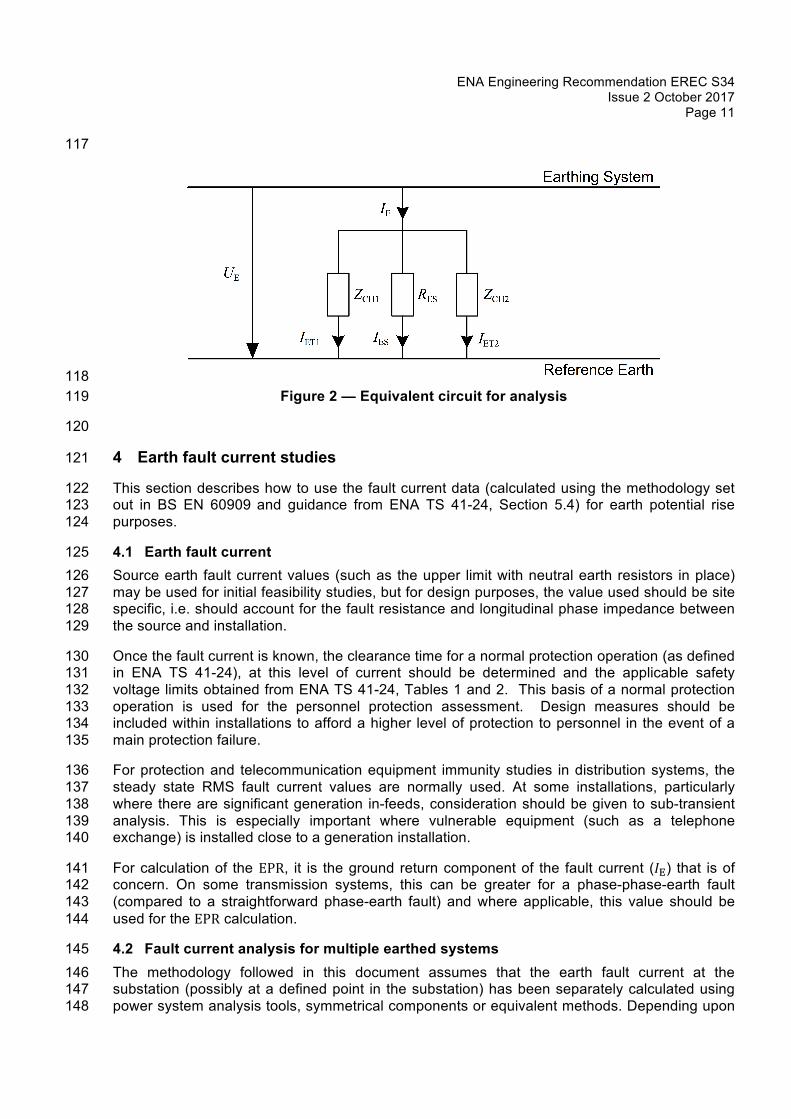
Page 31
Table 6 — Resultant fault current distribution and EPR(matrix method) 613
Parameter Value
𝐼%% 16.3 %
𝐼% 309 A
EPRB 442 V
6.2.5 Results 614 It can be seen that both methods give a reasonable correlation (𝐼%) = 318 A vs 309 A); minor 615 discrepancies will inevitably arise due to assumptions and approximations used with both 616 methods. In this case the C-factor method predicts a slightly higher EPR, and this will be used in 617 design calculations and discussion below. 618
A large proportion of the earth fault current returns via the cable sheaths. The current flowing 619 through the 1.43 Ω substation earth resistance creates an EPR of only 455 V (compared to 620 2144 V in case study 1), despite the higher overall fault current. The EPR is considerably lower 621 than the permissible touch voltage, so no further calculations are necessary. 622
The worst conceivable situation would involve the loss of the sheath connections co-incident 623 with the earth fault. (This is considered an unlikely event for triplex or three single-core circuits). 624 The EPR would increase to a theoretical maximum of around 2711 V (1.43 Ω x 1896 A) [in 625 practice the situation would be closer to 2144 V as calculated for Case Study 1 because the 626 fault current would reduce]. However, the foundation re-bar and perimeter electrode would 627 restrict the touch voltage to just 29 %, i.e. 621 V, which is much lower than the permissible 628 touch voltage of 944 V on chippings. The site would still be compliant in terms of safety 629 voltages, although there would now be a larger external zone with high surface potential. 630
6.3 Case study 3: 33 kV substation supplied via mixed overhead line/cable circuit 631
632
Figure 10 — Case study 3: Supply arrangement 633
This is a more complex example to demonstrate the issues involved in an area where there are 634 towns or villages supplied from an overhead line network. This example shows a 33 kV supply 635 but the arrangement is also very common at 11 kV; in both case an identical approach is used 636 for analysis using appropriate cable data. 637
The circuit length remains at 3 km, with 500 m of cable at each end and 2 km of overhead line 638 in the centre. The terminal poles at points C and D will have their own independent electrodes 639 (rods and/or buried earth wire) and are assumed to each have an earth resistance of 10 Ω for 640 insulation co-ordination purposes. 641
Substation A
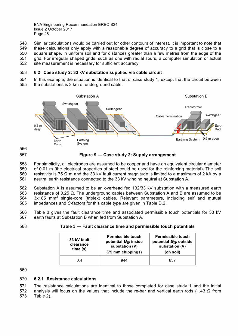
Switch
Earth Rods
0.6 m deep
Switchgear
Transformer
Substation B
Earthing System 0.6 m deep
150 m Electrode
Earthing System
C D

ENA Engineering Recommendation EREC S34 Issue 2 October 2017 Page 32
6.3.1 Resistance calculations 642 The resistance of Substation B is the same as calculated previously for a soil resistivity of 75 643 Ω·m. However, as is common practice, the opportunity has been taken to install a buried earth 644 wire with the incoming cable as shown. A length of 150 m is assumed and this will have a 645 resistance that will act in parallel with that of the grid. 646
Resistance of horizontal electrode: 647
Using formula R7, noting that the conductor length is smaller than the limit of validity given in 648 Table B.1: 649
𝑅, =𝜌
2𝜋𝐿,𝑙𝑜𝑔d
2𝐿,𝑑
650
depth of burial h=0.6, d =0.00944 m (approx. diameter of 70 mm2 conductor) 651
The resistance of the earth wire is 0.82 Ω. The resistance of the earth grid is 1.43 Ω. In parallel, 652 the combined resistance (ignoring proximity effects) is: 653
0.82 / 1.43 = 0.52 Ω 654
When proximity effects are included, by using a computer simulation software, the calculated 655 resistance value increases to 0.675 Ω. 656
6.3.2 Calculation of fault current and earth potential rise 657 The 33kV earth fault current is limited to a maximum of 2 kA by a neutral earthing resistor. The 658 impedance of the overhead line and cable arrangement further attenuates the fault current at 659 Substation B. The corresponding maximum earth fault current has been calculated to be 1594 A. 660
As this supply arrangement does not have a continuous metallic sheath back to the source, the 661 ground return current is calculated for the two 500 m sections of cable either side of the 662 overhead lines. The formulae from Appendix D and cable data in Table D.2 are used to 663 calculate the fault current distribution as shown in Figure 11. 664
665
Figure 11 — Case study 3: Equivalent circuit 666
In this example, the C-factor formula given in D.4.3 can be used to give the current split 667 between cable sheath return and ground return paths, from the perspective of substation B. 668

ENA Engineering Recommendation EREC S34 Issue 2 October 2017
Page 33
The current flows into soil (via 𝑅D), and along the cable sheath (via RD + the cable sheath 669 impedance). RD (10 Ω) is used in place of RA in the formula. In this case, 670
𝐼%)(D) = 𝐼3×
𝐶(𝑎 + 9𝐸) +
𝑅l
𝐶𝑎 + 9𝐸 +
𝑅Dl
.+ 0.6 𝜌
𝑎𝐸5.-
671
Results are shown in Table 7. 672
Table 7 — Input data and results for final part of circuit 673
Parameter Value
𝐸 33 kV
𝜌 75 W·m
a 185 mm2
C 67 (from Table D.2)
𝑅 10 W
𝑅D 0.675 W
RDB = RD + RB 10.675 Ω
l 0.5 km
𝐼3 1594 A
𝐼%)(D)% 93.6 %
𝐼%)(D) 1493 A
EPRB 1008 V
𝐼%)() 101 A
EPRD 1010 V
674
As shown in Table 7, 93.6 % of the available fault current flows through RB and creates an EPR 675 of 1008 V. The remainder of the current returns via the cable sheaths and through the earth 676 resistance at point D, creating a similar EPR at point D. 677
The companion C-factor formula given in D.4.2 can be used to calculate the EPR at the source 678 substation (Substation A) and the first pole/cable interface at C for the same fault at Substation 679 B. In this application, in the formula it is necessary to use RC in place of RB, and RAC = RA + RC in 680 place of RAB. 681
In this case, 682

ENA Engineering Recommendation EREC S34 Issue 2 October 2017 Page 34
𝐼%)(+) = 𝐼3×
𝐶(𝑎 + 9𝐸) +
𝑅+l
𝐶𝑎 + 9𝐸 +
𝑅C+l
.+ 0.6 𝜌
𝑎𝐸5.-
683
This shows that approximately 39.4 A is collected by the rod electrode at C, giving an EPR at C 684 of 39.4 x 10 = 394 V. 685
The remainder of the current (1554.6 A) returns via the ground to the source where it flows 686 through the 0.25 Ω resistance RA and creates an EPR at A of 389 V. 687
As shown in Table 8, the EPR at the source substation A is only 389 V. This is sufficiently low 688 that the calculation of touch, step and external impact contours is not required. The EPR at 689 Substation B exceeds the limits for soil and chipping surfaces, hence the calculation of touch, 690 step and external impact contours is required. 691
Although the EPR at terminal pole D is relatively high (1010 V), this may not pose a touch 692 potential hazard as the earth conductors on the pole are normally insulated. 693
Table 8 — Input data and results for initial part of circuit 694
Parameter Value
𝐸 33 kV
𝜌 75 W·m
a 185 mm2
C 67 (from Table D.2)
𝑅C 0.25 W
𝑅+ 10 W
𝑅C+ = 𝑅C + 𝑅+ 10.25 W
l 0.5 km
𝐼3 1594 A
𝐼%)(C)% 97.53 %
𝐼%)(C) 1554.6 A
EPRA 389 V
𝐼%)(+) 39.4 A
EPRC 394 V
695
6.4 Case study 4: Multiple neutrals 696 6.4.1 Introduction 697 In UK networks operating at voltages of 132 kV and above, the system neutral is generally 698 solidly and multiply earthed. This is achieved by providing a low impedance connection between 699

ENA Engineering Recommendation EREC S34 Issue 2 October 2017
Page 35
the star point of each EHV transformer (primary) winding and each substation earth electrode. 700 The low impedance neutral connection often provides a parallel path for earth fault current to 701 flow and this reduces the amount of current flowing into the substation earth electrode. For EPR 702 calculations in such systems, the neutral returning component of earth fault current should be 703 considered. The current split between the different return paths in this study is shown by red 704 arrows in Figure 12. 705 Circuits entering a substation are often via a mixture of overhead and underground cables. A 706 high percentage of the earth fault current flowing in an underground cable circuit will return to 707 source via the cable sheath if bonded at both ends (typically 70 % to 95 %), whereas in an 708 earthed overhead line circuit the current flowing back via the aerial earth wire is a lower 709 percentage (typically 30 % - 40 %). It is therefore necessary to apply different reduction factors 710 to the individual currents flowing in each circuit. The individual phase currents on each circuit 711 are required for these calculations. 712 The detailed fault current data required is normally available at transmission level from most 713 network modelling software packages. Any additional calculation effort at an early stage is 714 usually justified by subsequent savings in design and installation costs that result from a lower 715 calculated EPR. 716
This case study has been selected to illustrate: 717
a) Calculations to subtract the local neutral current in multiply earthed systems. 718 b) The application of different reduction factors for overhead line and underground cable 719
circuits. 720 c) A situation where there are fault infeeds from two different sources. 721 Figure 12 shows a simplified line-diagram of an arrangement where a 132 kV single phase to 722 earth fault is assumed at 132/33 kV Substation X. Two 132 kV circuits are connected to 723 Substation X, the first is via an overhead line from a 400/132 kV Substation Y and the second is 724 via an underground cable from a further 132/33 kV Substation Z which is a wind farm 725 connection. There is a single transformer at Substation X and its primary winding is shown 726 together with the star point connection to earth. 727
728 729 730 731 732 733 734 735 736 737 738 739 740 741 742
743 744
745 746 747
748 749
IB(Y)
3I0(Y) A C
IA(N) IB(N)IC(N)
Substation X
Overhead Line to
Substation Y IA(Z) Underground
Cable to Substation Z
IA(Y)
IC(Y)
B
IB(Z)Transformer (HV Winding)
IC(Z)
3I0(Z)
IN ISIETFault (IF )
Substation X Earthing System IES
RES
Reference Earth NOTE: Red arrows show current split from the fault point.
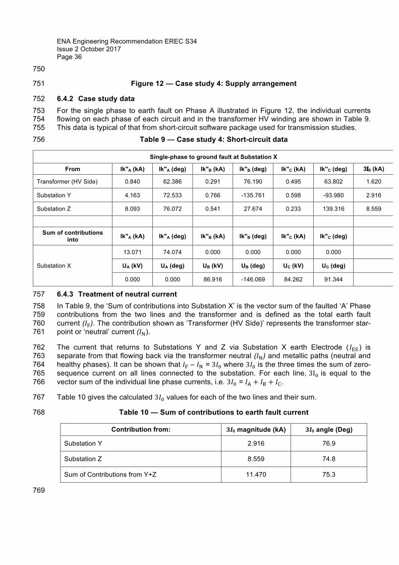
ENA Engineering Recommendation EREC S34 Issue 2 October 2017 Page 36
750
Figure 12 — Case study 4: Supply arrangement 751
6.4.2 Case study data 752 For the single phase to earth fault on Phase A illustrated in Figure 12, the individual currents 753 flowing on each phase of each circuit and in the transformer HV winding are shown in Table 9. 754 This data is typical of that from short-circuit software package used for transmission studies. 755
Table 9 — Case study 4: Short-circuit data 756
Single-phase to ground fault at Substation X
From Ik"A (kA) Ik"A (deg) Ik"B (kA) Ik"B (deg) Ik"C (kA) Ik"C (deg) 3I0 (kA)
Transformer (HV Side) 0.840 62.386 0.291 76.190 0.495 63.802 1.620
Substation Y 4.163 72.533 0.766 -135.761 0.598 -93.980 2.916
Substation Z 8.093 76.072 0.541 27.674 0.233 139.316 8.559
Sum of contributions into Ik"A (kA) Ik"A (deg) Ik"B (kA) Ik"B (deg) Ik"C (kA) Ik"C (deg)
Substation X
13.071 74.074 0.000 0.000 0.000 0.000
UA (kV) UA (deg) UB (kV) UB (deg) UC (kV) UC (deg)
0.000 0.000 86.916 -146.069 84.262 91.344
6.4.3 Treatment of neutral current 757 In Table 9, the ‘Sum of contributions into Substation X’ is the vector sum of the faulted ‘A’ Phase 758 contributions from the two lines and the transformer and is defined as the total earth fault 759 current (𝐼3). The contribution shown as ‘Transformer (HV Side)’ represents the transformer star-760 point or ‘neutral’ current (𝐼4). 761
The current that returns to Substations Y and Z via Substation X earth Electrode (𝐼%) ) is 762 separate from that flowing back via the transformer neutral (𝐼4) and metallic paths (neutral and 763 healthy phases). It can be shown that 𝐼3 – 𝐼4 = 3𝐼5 where 3𝐼5 is the three times the sum of zero-764 sequence current on all lines connected to the substation. For each line, 3I5 is equal to the 765 vector sum of the individual line phase currents, i.e. 3𝐼5 = 𝐼C + 𝐼D + 𝐼+. 766
Table 10 gives the calculated 3𝐼5 values for each of the two lines and their sum. 767
Table 10 — Sum of contributions to earth fault current 768
Contribution from: 3I0 magnitude (kA) 3I0 angle (Deg)
Substation Y 2.916 76.9
Substation Z 8.559 74.8
Sum of Contributions from Y+Z 11.470 75.3
769
ENA Engineering Recommendation EREC S34 Issue 2 October 2017
Page 37
From Table 9 and Table 10 it can be seen that earth fault current magnitude of 13.07 kA 770 calculated by the short-circuit software package reduces to 11.47 kA once the local neutral 771 current is subtracted. 772
As a further check of this value, the sum of the currents flowing on the transformer (HV Side) 773 can be subtracted from the total earth fault current calculated by the short-circuit software 774 package to arrive at the same result, i.e. 13.07Ð74° - 1.62Ð65.3° = 11.47Ð75.3° (kA) 775
6.4.4 Fault current distribution 776 The circuit from Substation Y is via an overhead line, whereas that from Substation Z is via an 777 underground cable. Further calculations are required to calculate the fault current distribution 778 between the substation electrode, tower line earth wire and the underground cable sheaths. 779
Table 11 lists the additional information assumed for this case study. 780
The calculated reduction factors (rE) for each circuit type from Table 11 are applied to the three-781 times zero-sequence currents (3𝐼5) on each circuit and the total ground return current (𝐼%) is 782 calculated. Results are given in Table 12. 783
The total ground return current magnitude (𝐼%) is shown to be only 1.5 kA which is significantly 784 lower than the short-circuit current at the fault point (𝐼3) of 13.07 kA. 785
Table 11 — Information for fault current distribution calculations 786
Line construction between Substations X and Y 132 kV double circuit tower line L4 construction. 20 spans long.
Reduction factor for line between Substations X and Y 0.708Ð-9° (From Table E.1)
Line construction between Substations X and Z 132 kV, 3 x 1c, 300 mm2 aluminium conductor, 135 mm2 copper-wire screen, XLPE insulated. 5 km circuit length.
Substation Y earth resistance 0.1 Ω
Substation X earth resistance 0.5 Ω
Reduction factor for cable between Substations X and Z 0.067Ð178° (From Table 12)
787
Table 12 — Calculated ground return current 788
Contribution From:
3𝑰𝟎 magnitude
(kA)
3𝑰𝟎 angle (deg)
rE Magnitude
rE angle (deg)
IES/IE magnitude
(kA)
IES/IE angle (deg)
Substation Y 2.916 76.9 0.708 -9 2.06 67.9
Substation Z 8.559 74.8 0.067 178 0.565 252.8
Sum of Contributions
from 11.470 75.3 1.50 66.1

ENA Engineering Recommendation EREC S34 Issue 2 October 2017 Page 38
Substations Y+Z
789
6.4.5 Earth potential rise (EPR) 790 The EPR can be calculated simply as the product of the ground return current 𝐼% and the overall 791 earth resistance 𝑅% at Substation X, i.e. 1.5 kA x 0.5 Ω = 750 V 792
6.5 Case study 5: 11 kV substation and LV earthing interface 793 A 500 kVA 11 kV unit substation is looped into two 11 kV, 185 mm2 aluminium triplex cables 794 with 35 mm2 copper screens, each 1 km long. Cable self and mutual impedances are taken 795 from Table D.2. One cable is connected to the 11 kV source and the other is feeding an open 796 11 kV ring. A cladding enclosure surrounds the substation and a concrete raft covers the 797 internal area of approximately 3x3 m. The soil resistivity is 50 Ω·m and the maximum fault 798 current for a single phase to earth fault is 3 kA. A fault clearance time of 1 s is assumed and the 799 corresponding permissible touch voltage (on soil) is 233 V. In this example, polymeric LV cables 800 are assumed to be employed which offer no effective contribution to earthing. 801
6.5.1 Design option 1 802 This preliminary design assumes an earth electrode comprising a perimeter horizontal bare 803 copper electrode (size 25 mm x 4 mm) around the plinth buried at a depth of 0.6 m with four 804 vertical rod electrodes connected at each corner. The rods are assumed to be 2.4 m long and 805 16 mm diameter. 806
807 808
Figure 13 — Case study 5: Option 1 809
Using formulae R4 to R6:
𝑅- = 𝑅%) =𝜌4𝑟+𝜌𝐿%
𝑅` =𝜌
2𝜋𝐿`𝑙𝑜𝑔d
8𝐿`𝑑
− 1
𝑅. = 𝑅%` = 𝑅`1 + 𝑘𝛼𝑁
𝛼 =𝜌
2𝜋𝑅`𝑠
𝐿% = length of horizontal electrode
𝐿` =rod length
d= diameter. Valid for d<<𝐿`
𝑟 =𝐴𝜋
𝑁 = total number of rods = 4; 𝑘 and 𝛼
11 kV Open Ring
Substation A GRP Unit Substation B
Cable (1 km) Cable (1 km)

ENA Engineering Recommendation EREC S34 Issue 2 October 2017
Page 39
𝑅-. = 𝑅- −𝜌𝜋𝐿%
𝑙𝑜𝑔d𝐿`𝑏− 1
𝑅% = 𝑅-𝑅. − 𝑅-..
𝑅- + 𝑅. − 2𝑅-.
Therefore:
𝑅- =50
4×1.69+5012
= 11.56Ω
𝑅` =50
2𝜋×2.4(logd(
8×2.40.016
) − 1) = 20.19Ω
𝛼 =50
2𝜋×20.19×3= 0.13
𝑅. = 20.19×1 + 2.6×0.13
4= 6.75Ω
𝑅-. = 11.56 −50
𝜋×12𝑙𝑜𝑔d
2.40.01
− 1 = 5.62Ω
𝑅% =11.56×6.75 − 5.62.
11.56 + 6.75 − 2×5.62= 6.57Ω
defined below.
A= area of grid (m2)
𝑠 is the distance between rods (m)
2.4 m rod length, 16 mm diameter.
k = 2.6 for 4 rods (From Figure B.1)
810 As this is a preliminary design, several conservative assumptions can be made. The source 811 resistance is assumed to be 0.1 Ω and the attenuation of fault current by the earth resistance 812 and circuit impedance is neglected at this stage. 813
6.5.2 C-factor method 814 This arrangement (all cable circuit) is shown in Figure D.1. 815
𝐼% = 𝐼3×
𝐶(𝑎 + 9𝐸)
𝐶𝑎 + 9𝐸 +
𝑅CDl
.+ 0.6 𝜌
𝑎𝐸5.-
816
817

ENA Engineering Recommendation EREC S34 Issue 2 October 2017 Page 40
Table 13 —Option 1 input data and results 818
Parameter Value
𝐸 11 kV
𝜌 50 W·m
a 185 mm2
𝐶 47 (from Table D.2)
𝑅C 0.1 W
𝑅D 6.57 W
𝑅CD= RA+RB 6.67 W
l 1 km
𝐼3 3000 A
𝐼%% 2.41 %
𝐼% 72.3A
EPRB 475 V
6.5.3 Matrix method 819 This method is appropriate where cable physical parameters are available. Self and mutual 820 impedance values can be determined from data provided by manufacturers (or from 821 measurements) and by using formulae in Appendix D. 822
The fault current distribution and calculated EPR associated with the source 11 kV cable, 823 calculated for option 1 using the formulae in Appendix D is shown in Table 14. 824
Table 14 — Resultant fault current distribution and EPR (matrix method) 825
Parameter Value
𝐼%% 2.41 %
𝐼% 72.3 A
EPRB 475 V
6.5.4 Results 826 It can be seen that both methods give identical results. The EPR exceeds 2 x UTP (2 x 233 V = 827 466 V) and therefore segregation of HV/LV earthing systems is required. 828
6.5.5 Surface current density 829 The surface current density of the earth electrode for the fault conditions listed above should be 830 evaluated and compared with the limit of surface current density, provided by Formula C2 as 831 shown below: 832
𝐽|?| = 10057.7𝜌𝑡
-/.
833

ENA Engineering Recommendation EREC S34 Issue 2 October 2017
Page 41
i.e.: 834
𝐽|?| = 100 ¡.¡ 5×
-/.= 0.62×100 A/mm2 (t= 3 s) 835
The total electrode surface area is: 836
Horizontal electrode surface area = 696 × 103 mm2 837
Vertical rod surface area = 483 × 103 mm2 838
Total electrode surface area = 1180 × 103 mm2 839
Assuming a uniform current distribution throughout the earthing system, the actual current 840 density is: 841
𝐽 = ¡..--£5×-5¤
= 61.3×100¥ A/mm2 842
Based on the above, the actual current density is below the limit of surface current density, 843 hence the amount of electrode installed is adequate. The electrode will remain within limits for a 844 total ground return current up to 731 A. The impact of this limit should be considered for future 845 planning i.e. increased fault levels or loss of sheath connection. 846
6.5.6 Design option 2 847 A second design is considered and comprises the arrangement described in option 1 together 848 with a bare stranded electrode buried with each 11 kV cable for a distance of 20 m and 849 connected to the substation earthing system. 850
851 852
Figure 14 — Case study 5: Option 2 853
The resistance of each extended horizontal electrode can be calculated using Formula R7: 854
𝑅, =𝜌
2𝜋𝐿,𝑙𝑜𝑔d
2𝐿,𝑑
855
856
𝑅%, =50
2𝜋×20𝑙𝑜𝑔d
2×200.00944
= 3.3Ω. 857
Ignoring proximity effects, the combined parallel resistance for the substation and both 858 horizontal electrodes is 1.33 Ω. Using the same basic assumptions as Section 6.5.1, the fault 859 current distribution and EPR for the earthing arrangement, calculated using the two methods 860 provided in Appendix D, is given in Table 15 and Table 16. 861
862
Cable (1 km) Cable (1 km)
Substation A
GRP Unit Substation B
20 m Electrode
11 kV Open Ring
20 m Electrode

ENA Engineering Recommendation EREC S34 Issue 2 October 2017 Page 42
6.5.7 C-factor method 863 This arrangement (all cable circuit) is given in Figure D.1. 864
𝐼% = 𝐼3×
𝐶(𝑎 + 9𝐸)
𝐶𝑎 + 9𝐸 +
𝑅CDl
.+ 0.6 𝜌
𝑎𝐸5.-
865
866
Table 15 — Option 2 input data and results 867
Parameter Value
𝐸 11 kV
𝜌 50 W·m
a 185 mm2
𝐶 47 (from Table D.2)
𝑅C 0.1 W
𝑅D 1.33 W
𝑅CD = RA+RB 1.43 W
l 1 km
𝐼3 3000 A
𝐼%% 9.62 %
𝐼% 278 A
EPRB 361 V
868
6.5.8 Matrix method 869 This method is appropriate where cable physical parameters are available. Self and mutual 870 impedance values can be determined from data provided by manufacturers (or from 871 measurements) and by using formulae in Appendix D. 872
The fault current distribution and calculated EPR associated with the source 11 kV cable 873 calculated for option 2 using the formulae in Appendix D is given in Table 16. 874
Table 16 — Resultant fault current distribution and EPR (matrix method) 875
Parameter Value
𝐼%% 8.27 %
𝐼% 248 A
EPRB 394 V

ENA Engineering Recommendation EREC S34 Issue 2 October 2017
Page 43
876
6.5.9 Results 877 Table 15 and Table 16 demonstrate that the EPR based on the second preliminary design is 878 below the 466 V permissible touch voltage and therefore a combined HV/LV earthing system 879 can be installed. 880

ENA Engineering Recommendation EREC S34 Issue 2 October 2017 Page 44
APPENDICES 881
A Symbols used within formulae or figures 882
B Formulae 883
C Earthing design methodology (block diagram) 884
D Formulae for determination of ground return current for earth faults on metal sheathed 885 cables 886
E Ground current for earth faults on steel tower supported circuits with aerial earth wire 887
F Chart to calculate resistance of horizontal electrode 888
G Chain impedance of standard 132 kV earthed tower lines 889
H Sample calculations showing the effect on the ground return current for change in the 890 separation between three single-core cables 891
I Transfer potential from HV systems to LV systems with multiple earthed neutral 892
893

ENA Engineering Recommendation EREC S34 Issue 2 October 2017
Page 45
Appendix A Symbols used within formulae or figures 894
(Those shown in Old column were used in earlier versions of this document, but have been 895 updated to align as far as possible with BS EN 50522:2010). 896
New Old Symbol Description
a Conductor cross-sectional area (mm2)
𝑏 𝑏 equivalent diameter of circular electrode (m)
C ‘C’ factor used to calculate split of current between ground and metallic return paths (cable sheaths)
CH CH chain (or ladder) network of an overhead line earth wire with its connections to earth via metal lattice towers along its route, or an insulated cable’s sheath that has connections to earth via installations along its length
𝑑 𝑑 diameter of circular electrode (or width of tape electrode) (m)
𝐷 𝐷 average spacing between parallel grid electrodes (m)
E System voltage (kV)
ℎ h radius of equivalent hemisphere (m)
𝐼% 𝐼§¨ component of 𝐼3 that flows through the electrode network and eventually all returning through the ground (A)
𝐼%) 𝐼© component of 𝐼3 passing to ground through grid electrode (A)
𝐼%7 𝐼ª component of 𝐼% passing to ground through tower footing (A)
𝐼3 𝐼« total earth fault current (A)
𝐼¬ 𝐼 component of 𝐼% passing to ground through external horizontal electrode (A)
𝐼4 𝐼® current via local transformer neutral (A)
𝐼¨ 𝐼¨ component of 𝐼3 through remote transformer neutrals (A)
𝐼) 𝐼 ¨ component of 𝐼3 returning through earth wire or cable sheath (A)
𝐽|?| Limiting current density (A/mm2 of electrode surface area)
𝑘 𝑘 geometric coupling factor or arrangement factor
l 𝑙𝑜𝑟𝐿+ cable length (km)
𝐿% L or 𝑙E total length of electrode (e.g. in grid, not including rods) (m)
𝐿, 𝑙H horizontal electrode length (m)

ENA Engineering Recommendation EREC S34 Issue 2 October 2017 Page 46
New Old Symbol Description
𝐿@ 𝑙P grid or loop electrode length (perimeter) (m)
𝐿` 𝑙R length of earth rod (m)
𝐿7 total electrode length, including horizontal electrode and summated rod lengths (m)
rE 𝑟© reduction factor of the overhead line
𝜌 ρ earth resistivity (W·m)
𝑟° 𝑟± cable armour resistance per unit length (W/km)
𝑅C earthing resistance at substation A (W)
𝑅D earthing resistance at substation B (W)
𝑟< rc cable sheath resistance per unit length (W/km)
𝑅% 𝑅d total earthing resistance at substation (W) [or resistance of specific electrode]
𝑅%, 𝑅 external horizontal electrode earthing resistance (W)
𝑅%² 𝑅³ earth plate resistance (W)
𝑅%` R2 resistance of group of rods (W)
𝑅%) RI and Rg grid electrode earthing resistance (W)
𝑅%7 𝑅ª tower footing resistance (W)
𝑅´ Rf fault resistance (W)
𝑅4% Rne neutral earthing resistance (W)
𝑅` resistance of single rod (W)
s S line span length (km)
UE Ve rise of earth potential of substation (V)
US step potential (V)
USP permissible step potential (V)
UT touch potential (V)
UVS prospective step potential (V)

ENA Engineering Recommendation EREC S34 Issue 2 October 2017
Page 47
New Old Symbol Description
UVT prospective touch potential (V)
UTP permissible touch voltage (V)
𝜑 Phase angle (degrees or radians)
𝑉x VS voltage on the surface of the soil at point S (point x), with respect to true earth potential (V)
VT transfer potential (V)
x distance to point where voltage on soil is Vx (m)
𝑍+ zc (cable sheath impedance) - the impedance of the overall sheath and armour of 3-core cables, or of all three sheaths of 3 × single-core cables, per unit length (W/km)
𝑍+, 𝑍· chain (or ladder) network impedance (W) (Referred to as Zp in BS EN 60909-3; referred to as Z∞ in BS EN 50522:2010)
𝑍% Ze impedance to earth, substation earthing impedance (W)
zmp,1 zmp,1 )
zmp,2 zmp,2 mutual impedance between cable conductor and sheaths 1, 2 and 3 respectively of three single-core cables (W/km)
zmp,3 zmp,3 )
zml,2 zmp,2 )
zml,3 zmp,3 mutual impedance between sheaths 1, 2 and 3 of three single-core cables (W/km)
zm2,3 zmp,3 )
zmp,s zmp,s mutual impedance between line conductor and earth wire (W/km)
zmp,c zmp,c mutual impedance between cable conductor and sheath of three-core cables (W/km)
𝑍» tower line earth wire impedance per unit length (W/km)
𝑧¯ earth wire impedance per unit length (W/km)
Ð Ð angle in degrees
897

ENA Engineering Recommendation EREC S34 Issue 2 October 2017 Page 48
Appendix B Formulae 898
Symbols are as given in Appendix A unless otherwise re-defined in this Appendix. 899
Formulae in this section are those which are considered most relevant to UK network operators. 900 They may differ from those in BS EN 50522 where they are known to be a simplification and/or 901 restricted in their application. 902
See BS 7430 for additional formulae related to simple rod arrangements that would not 903 generally be used at distribution or transmission network operator installations. 904
The formulae have been grouped as follows: 905
R = earth resistance of different arrangements. 906
C = current rating. 907
P = potentials (surface, touch and step). 908
B.1 Earth resistance formulae (R) 909
B.1.1 Formula R0: Hemispherical electrode 910
𝑅% =𝜌2𝜋𝑟
where: r= radius of hemisphere (m)
911
B.1.2 Formula R1: Rod electrode 912
𝑹𝐑 =𝝆
𝟐𝝅𝑳𝐑𝒍𝒐𝒈𝒆
𝟖𝑳𝐑𝒅
− 𝟏
valid for𝑳𝐑 ≫ 𝒅/𝟐
B.1.3 Formula R2: Plate electrode (mainly used for sheet steel foundations) 913
𝑅%² =𝜌8𝑟
1 +𝑟
2.5ℎ + 𝑟
where: 𝑟 =
𝐴𝜋
𝐴 = area of one face of the plate (m2)
ℎ = depth of burial (m)
B.1.4 Formula R3: Ring electrode 914
𝑅% =𝜌
4𝜋.𝑟𝑙𝑜𝑔d
64𝑟.
𝑑ℎ
where:
ℎ = depth (m)
𝑟 = ring radius (m) = Ê
𝑑= conductor diameter (m)

ENA Engineering Recommendation EREC S34 Issue 2 October 2017
Page 49
B.1.5 Formula R4: Grid/mesh resistance 915
𝑅%) =𝜌4𝑟+𝜌𝐿%
where: 𝑟 =
𝐴𝜋
A = area of grid (m2) 𝐿%= total length of buried conductor excluding rods (m)
B.1.6 Formula R5: Group of rods around periphery of grid 916
𝑅%` = 𝑅`1 + 𝑘𝛼N
where: RR = Resistance of one rod (Ω) (Formula R1)
𝛼 =𝜌
2𝜋𝑅`s
s = spacing of rods (m)
N = total number of rods around periphery of grid
k = factor from Figure B.1 below
917 Figure B.1 — factor k for formula R5 918
919
B.1.7 Formula R6: Combined grid and rods (rods on outside only) 920
𝑅% = 𝑅-𝑅. − 𝑅-..
𝑅- + 𝑅. − 2𝑅-.
where: 𝑅- = 𝑅%)= resistance of grid (Formula R4)
𝑅. = 𝑅%` = resistance of group of rods around periphery of grid (Formula R5)

ENA Engineering Recommendation EREC S34 Issue 2 October 2017 Page 50
𝑅-. = 𝑅- −𝜌𝜋𝐿%
𝑙𝑜𝑔d𝐿`𝑏− 1
𝑏 = 𝑤/𝜋 where:
𝑤 = width of tape electrode (m) 𝐿% = length of buried conductor excluding rods (m)
𝐿` = rod length (m)
NOTE: The formula gives sensible results only for generally used dimensions – in particular for normal rod 921 widths/diameters and spacing. 922
B.1.8 Formula R7: Strip/tape electrode 923
For horizontal electrodes, the following formula (from BS EN 50522) may be used: 924
𝑅, =𝜌
2𝜋𝐿,𝑙𝑜𝑔d
2𝐿,𝑑
where: depth of burial = 0.5 to 0.6 m
d = diameter of round conductor or half-width of tape (m)
The above formula is valid for 𝐿, ≫ 𝑑and 𝐿, ≤ 60√𝜌 (see Table B.1). 925
With increasing electrode length, there will be a point after which the effect of adding further 926 length is significantly diminished due to the self-impedance of the electrode that is not 927 accounted for. These lengths for a single earth wire, tape or PILCSWA cable are shown in 928 Table B.1. The behaviour with length of the resistance of long horizontal conductors 𝑅%, is 929 illustrated by the typical values shown in Figure F.1. 930
Table B.1 - Approximate lengths for a single horizontal earth wire, tape or PILCSWA 931 cable beyond which no further significant reduction in resistance can be obtained 932
Soil resistivity ρ (Ω·m)
Length 𝑳𝐇(m) = 𝟔𝟎√𝝆
1 60
10 190
100 600
1000 1900
933
In cases where there are several conductors in reasonably close proximity, computer software 934 or a more detailed formula (such as Schwarz [4]) should be used. The advantage of using 935 computer software is that the extended electrode cross sectional area and material can be 936 correctly accounted for. 937
938

ENA Engineering Recommendation EREC S34 Issue 2 October 2017
Page 51
939
B.1.9 Formula R8: Ladder networks 940
NOTE: In Formulae R8.1 and R8.2 below, quantities are complex impedances, rather than magnitudes. For triplex 941 cables, or single-core cables, the combined sheath resistance will be the parallel value, but the reactance should be 942 calculated for the dimensions/spacing for them to act as an equivalent single sheath conductor. For circuits feeding 943 the fault, mutual coupling between the faulted phase conductor and the sheath(s) etc. also plays a significant role. In 944 many circumstances calculating these effects will not be practicable; the formulae should therefore be used only to 945 provide an approximation in such circumstances. More accuracy can be achieved by the use of appropriately 946 modelled sheath impedance data (e.g. provided by manufacturer), or by using a computer program that is able to 947 calculate the parameters from the physical properties of each cable section. 948 949 Formula R8.1: Long overhead lines with earth wire (BS EN 60909-3, 2010) 950
𝑍+, = 0.5𝑍» + (0.5𝑍»). + 𝑅%7 ⋅ 𝑍»
where: See BS EN 60909-3 for description of ZQ.
NOTE: Appendix G gives calculated values of ZCH for a traditional UK 132 kV tower line. 951 Formula R8.2: Long cable circuit with distributed earthed nodes (distribution substation 952 electrodes) (BS EN 60909-3) 953
𝑍+, =𝑍- + 𝑍-. + 4 ⋅ 𝑍- ⋅ 𝑍.
2
where: 𝑍- = equivalent longitudinal sheath impedance of cable connecting the substations. For single-core or triplex cables, this should take into account spacing/geometry between single-core cables.
𝑍. = average substation earthing impedance
0𝑗 + 𝑅D Ω
954
Formula R8.3: Short overhead lines with earth wire (typically 5 to 20 towers) 955
𝑍+, =𝑍Ó 𝑍©Ô +𝑍Ó 𝑘J + (𝑍Ó − 𝑍Õ)(𝑍©Ô − 𝑍Ó + 𝑍Õ)𝑘0J
𝑍©Ô + 𝑍Ó 𝑘J − (𝑍©Ô − 𝑍Ó + 𝑍Õ)𝑘0J
NOTE 1: All impedances are in complex notation. Formula as provided in (BS EN 60909-3). 956 NOTE 2: Refer to BS EN 60909-3 for descriptions of symbols, as they differ from those used in this document. 957 For detailed calculations, a discrete ladder network (iterative) routine or computer software 958 should be used. The self and mutual impedance for the earth wire(s) should be calculated 959 accounting for their material, cross sectional area and the circuit geometry. 960
Short underground cable/substation arrangements 961
Where a significant proportion of the cable is PILCSWA, the resistance is calculated based 962 entirely on this, using Formula R7. 963
Where the majority of the cable is XLPE/EPR/Triplex etc., an approximate approach is to treat 964 all the substation earth resistances as being in parallel and inflate the result by 30 % to account 965 for the longitudinal sheath impedance. This is sufficiently accurate for typical cable lengths of 966 200 m to 450 m and low sheath impedance. If more than 6 substations are to be considered, a 967

ENA Engineering Recommendation EREC S34 Issue 2 October 2017 Page 52
higher inflation amount needs to be considered. Detailed calculations will be needed if the 968 substation earth resistances approach 1 Ω or less, because the sheath impedance then 969 becomes significant. For detailed calculations, a discrete ladder network (iterative) routine or 970 computer software should be used. 971
See also BS EN 60909-3 for more details of the calculations for ladder networks, including non-972 symmetrical arrangements. 973
B.1.10 Formula R9: Accounting for proximity effects 974
The resistance 𝑅 (Ω) of n vertically driven rods set s metres apart may be calculated from: 975
𝑅 =1𝑛
𝜌2𝜋𝐿`
𝑙𝑜𝑔d8𝐿`𝑑
− 1 +l𝐿`𝑠
where: 𝜌 = is the resistivity of soil, in ohm metres (W·m)
𝐿` = is the length of the electrode, in metres (m); 𝑛 = is the number of rods;
𝑠 = is the spacing between rods
l = a group factor where: l = 2S(-.+ ⋯+ -
J)
NOTE: For larger values of n, l can be approximated by: l ~ 2 log× -.¡£-Ø..£-£
See Bibliography, reference [3]. 976
B.1.11 Formula R10: Overall earth resistance 977
𝑍% =1𝑅%)
+1
𝑍+,-+
1𝑍+,.
+ ⋯0-
978 NOTE: The overall impedance of an earthing system can be approximated to the parallel combination of all 979 component parts. This formula neglects proximity effects (overlapping resistance areas) and will generally provide a 980 lower value for 𝑍% than might be observed in practice (or provided by simulation results). 981 Computer software is best used to account for proximity effects e.g. where strip electrodes or 982 PILCSWA type cables run in parallel. 983
B.2 Current formulae 984
B.2.1 Formula C1: Current rating formula 985
For fault currents which are interrupted in less than 5 s the cross-section of earthing conductor 986 or earth electrode shall be calculated from the following formula: 987
𝐴 =𝐼𝐾
𝑡Ú
𝑙𝑜𝑔d𝛩Ú + 𝛽𝛩Ý + 𝛽
where: 𝐴 = cross-section (mm2)
𝐼 = conductor current (A) (RMS value) 𝑡Ú = duration of the fault (s)
𝐾 = a constant depending on the material of the current-carrying component; Table D.1 of IEC 60949 provides values for the most common materials assuming an initial temperature of 20 °C
𝛽 = reciprocal of the temperature coefficient of resistance of the current-carrying component at 0 °C.
𝛩Ý = initial temperature in degrees Celsius. Values

ENA Engineering Recommendation EREC S34 Issue 2 October 2017
Page 53
may be taken from (IEC 60287-3-1). If no value is laid down in the national tables, 20 °C as ambient ground temperature at a depth of 1 m should be adopted.
𝛩Ú = final temperature (°C)
(See IEC 60949, formula D1)
NOTE: Care should be taken not to exceed safe temperatures for cable sheaths (and their insulation), particularly on 988 heavily loaded circuits where the initial temperature may be close to 90 ºC. 989 990
B.2.2 Formula C2: Limit of surface current density formula 991
Actual current density: 992
SurfaceCurrentDensity = ©®d·ª¨ÞudßਨdJª¯à¨Ú±·d¨d±ÞÚ©®d·ª¨Þud
(A/mm2)
Limiting current density: 993
𝐽|?| = 100 ¡.¡áª
-/. (A/mm2)
where: 𝜌 = soil resistivity (Ω·m) 𝑡 = fault duration (s)
B.3 Surface potential formulae (P) 994
For substations with separately earthed fence and normal buried grid depths (typically 0.5 m): 995
B.3.1 Formula P1: External touch potential at the edge of the electrode 996
𝑈7 =𝑘d ∙ 𝑘u ∙ 𝜌 ∙ 𝐼%
𝐿7V
where: 𝑘d = factor that allows for the effect of a uniformly distributed electrode current over the grid (see below) 𝑘u = factor, which modifies 𝑘d to allow for the non-uniform distribution of electrode current (see below)
𝜌 = soil resistivity (W m) 𝐼% = total current passing to ground through electrode (A) 𝐿7 = total length of buried electrode conductor including rods if connected (m)
𝑘d =1𝜋
12𝑙𝑜𝑔d
ℎ𝑑+12ℎ
+1
0.5 + D+1D1 − 0.5J0.
ℎ = grid depth (m)
𝑑 = equivalent diameter of conductor = circumferenceofconductorπ
(m)
D = average spacing between parallel grid conductors (m)

ENA Engineering Recommendation EREC S34 Issue 2 October 2017 Page 54
𝑛 = 𝑛C×𝑛D-.
where 𝑛C = number of parallel grid conductors in one direction where 𝑛D = number of parallel grid conductors in the other direction
𝑘u = 0.7 + 0.3𝐿7𝐿@
where: 𝐿7 = total length of buried electrode conductor including rods if connected (m) 𝐿@ = perimeter length of buried electrode conductor including rods if connected (m)
𝑈7 = resulting touch potential or, when assessing length 𝐿, the permissible touch potential from ENA TS 41-24, Table 1
B.3.2 Formula P2: External touch potential at the fence 997
The ground current density is significantly diminished at the fence compared to that at the edge 998 of the grid electrode. As a result, a new factor, 𝑘Ú, based on a 2 m separation between fence 999 and grid electrode, is applied in place of 𝑘d in the above formulae. 1000
Hence: 1001
𝑈7(´×Ø<×) =𝑘Ú ∙ 𝑘u ∙ 𝜌 ∙ 𝐼%)
𝐿² V
Or, rearranged: 1002
𝐿² =𝑘Ú ∙ 𝑘u ∙ 𝜌 ∙ 𝐼%)
𝑈7(m)
where: 𝑘Ú= 0.26𝑘d (based on 2 m separation)
There are two situations to be considered. The first is where the fence is situated at the edge of 1003 the substation electrode. The second has a peripheral electrode conductor buried 0.5 m below 1004 the surface, 1 m beyond the fence and regularly bonded to it: 1005
B.3.3 External touch potential at fence with no external peripheral electrode: 1006
𝑈7(´×Ø<×) is the same as 𝑈7(z|)using formula P1 as above. 1007
B.3.4 Formula P3: External touch potential at fence with external buried peripheral 1008 conductor 1 m from fence 1009
𝑈7(´×Ø<×) =𝑘Úd ∙ 𝑘u ∙ 𝜌 ∙ 𝐼%)
𝐿² V 𝑜𝑟𝐿Ó =
𝑘Úd ∙ 𝑘u ∙ 𝜌 ∙ 𝐼%)𝑈7(´×Ø<×)
(m)
Where:
𝑘Úd =12𝑙𝑜𝑔d
ℎ𝑑−14𝑙𝑜𝑔d 𝑆. + 0.5. . +
14𝑙𝑜𝑔d 𝑆y + 𝑆.
ℎ and 𝑑 are as in formula P1;

ENA Engineering Recommendation EREC S34 Issue 2 October 2017
Page 55
𝑆 = distance between the outermost buried grid conductor and the next nearest parallel conductor (m). 1010
B.3.5 Formula P4: Touch potential within grid (from IEEE 80) 1011
The touch potential within the earth grid may be calculated using the following formulae from 1012 IEEE 80, Annex D, where it is defined as the mesh voltage. It is the touch potential that would 1013 be experienced at the centre of a corner mesh in an earth grid with an equally spaced mesh. 1014
NOTE: Terms used in these formulae are not defined in the rest of this document, and are included here for 1015 consistency with the source document (IEEE 80). 1016
𝐸ê =𝜌×𝐼©¯×𝐾ê×𝐾Ý
𝐿ß + 1.55 + 1.22× 𝐿¨
𝐿. + 𝐿ë.×𝐿q
𝐾ê =1
2×𝜋× 𝑙𝑛
𝐷.
16×ℎ×𝑑+
𝐷 + 2×ℎ .
8×𝐷×𝑑−
ℎ4×𝑑
+𝐾ÝÝ𝐾
×𝑙𝑛8
𝜋 2×𝑛 − 1
𝐾Ý = 0.644 + 0.148×𝑛 𝑛 = 𝑛±×𝑛ì×𝑛·×𝑛u
𝑛± =2×𝐿ß𝐿³
𝑛ì = 1𝑓𝑜𝑟𝑠𝑞𝑢𝑎𝑟𝑒𝑔𝑟𝑖𝑑𝑠, 𝑜𝑡ℎ𝑒𝑟𝑤𝑖𝑠𝑒:𝑛ì =𝐿³
4× 𝐴
𝑛· = 1𝑓𝑜𝑟𝑠𝑞𝑢𝑎𝑟𝑒𝑎𝑛𝑑𝑟𝑒𝑐𝑡𝑎𝑛𝑔𝑢𝑙𝑎𝑟𝑔𝑟𝑖𝑑𝑠, 𝑜𝑡ℎ𝑒𝑟𝑤𝑖𝑠𝑒:𝑛· =𝐿×𝐿ë𝐴
5.¡×ðñ×ðò
𝑛u = 1𝑓𝑜𝑟𝑠𝑞𝑢𝑎𝑟𝑒, 𝑟𝑒𝑐𝑡𝑎𝑛𝑔𝑢𝑙𝑎𝑟𝑎𝑛𝑑𝐿 − 𝑠ℎ𝑎𝑝𝑒𝑑𝑔𝑟𝑖𝑑𝑠, 𝑜𝑡ℎ𝑒𝑟𝑤𝑖𝑠𝑒:𝑛u =𝐷ê
𝐿. + 𝐿ë.
𝐾 = 1 +ℎℎ5
𝐾ÝÝ = 1 (for grids with numerous earth rods, especially where they are located at the corners and around the perimeter)
𝐾ÝÝ =-
.×Jôõ (for grids with no (or very few) earth rods, especially where they are not located
on corners or around the perimeter)
where: 𝐸ê = the mesh voltage (V) 𝜌 = the average soil resistivity (Ω·m) 𝐼©¯ = electrode current (A)

ENA Engineering Recommendation EREC S34 Issue 2 October 2017 Page 56
𝐿ß = total length of horizontal conductor in the grid (m) 𝐿q = total length of all earth rods (m) 𝐿¨ = average earth rod length (m) 𝐿³ = length of the perimeter conductor (m)
𝐿 = maximum length of the grid in the x direction (m) 𝐿ë = maximum length of the grid in the y direction (m)
𝐷 = spacing between parallel conductors in the mesh (m) 𝑑 = diameter of the earth conductors (m) ℎ = grid burial depth (m) 𝐴 = area of the grid (m2) 𝐷ê = maximum distance between any two points on the grid (m) ℎ5 = grid reference depth of 1 m
B.3.6 Formula P5: Step potential on outside edge of grid 1017
US =𝜌𝐼32𝜋𝑟
𝑎𝑟𝑐𝑠𝑖𝑛𝑟𝑥− 𝑎𝑟𝑐𝑠𝑖𝑛
𝑟𝑥 + 1
where: 𝑟 =𝜌
4𝑅%)
𝑥 = distance from centre of grid
B.3.7 Formula P6: Voltage profile around earth electrode 1018
Column P6.1 P6.2 P6.3
Electrode description Hemisphere Vertical rod Buried grid
Configuration, where I = injected current.
Voltage 𝑉with respect to true earth on the
surface of the ground at distance 𝑥
for 𝑥 >r
𝑉 =𝜌. I2𝜋𝑥
= 𝑈©𝑟𝑥
for𝑥 > 𝑑/2
𝑉 =á.÷.Êðø
logdðø+ 1 + ðøô
ô
= 𝑈© 𝜌
2𝜋𝐿`𝑅`logd
𝐿`𝑥+ 1 +
𝐿`.
𝑥.
for 𝑥 >r
𝑉 =𝜌. I2𝜋𝑟
arcsin𝑟𝑥
=2𝑈𝐸𝜋
arcsin𝑟𝑥
where: 𝑟 = áyqúû
and
arcsin ¨ is in radians
LR

ENA Engineering Recommendation EREC S34 Issue 2 October 2017
Page 57
1019
B.3.8 Formula P7: Calculation of specific external potential contours 1020
𝑥 =𝐴𝜋
𝑠𝑖𝑛𝑉𝜋2𝑈%
0-− 1
where: 𝑥 = distance (m) from edge of grid (effective radius 𝑟) to a point where the surface potential is 𝑉 (V)
𝐴 = 𝜋𝑟2 (m2), where 𝑟 = áyqúû
(see Formula P.6.3)
𝑈% = earth potential rise (V)
NOTE: Angles are in radians. 1021 These formulae apply on the basis that the earthing installation may be treated as equivalent to 1022 a symmetrical grid. 1023
Substation fences are usually earthed independently from the main earthing system and may be 1024 up to 2 m from it. By using the above formulae to calculate the radius of any voltage contour, a 1025 factor of safety is introduced when they are measured from the substation fence. Some 1026 discretion may be necessary in assessing the radius from a substation where the fence is 1027 bonded to the earthing installation or there is a large distance from the fence to the edge of the 1028 earthing system. 1029
Clearly, this formula does not apply when 𝑈% is lower than the voltage contour of interest. 1030

ENA Engineering Recommendation EREC S34 Issue 2 October 2017 Page 58
Appendix C Earthing design methodology 1031
1032

ENA Engineering Recommendation EREC S34 Issue 2 October 2017
Page 59
Appendix D Formulae for determination of ground return current for earth faults 1033 on metal sheathed cables 1034
D.1 Introduction 1035
The current in the core of a single-core cable or the unbalance of current in the cores of a 1036 multicore cable induces a voltage in the metallic sheath/armour of the cable. If the 1037 sheath/armour is connected to earth at each end of its length, a current will be driven through 1038 the sheath/armour earth loop which constitutes part of the earth fault current returning from the 1039 fault, the remainder being that returning in the ground. The quantity of current returning in the 1040 cable sheath/armour is, inter alia, dependent on the location of the cable in the system with 1041 respect to the source of fault current infeed and to the position of the fault as well as on the 1042 values of the sheath/armour terminating earth resistances. 1043
Formulae for the computation of the ground current are given below, in respect of a cable 1044 terminated and earthed at points A and B. These are based upon circuit models including the 1045 self and mutual impedances between the different physical conductors (cores, sheaths, 1046 screens). The arrangements considered are illustrated in Figures D.1 to D.4. 1047
Alternative formulae are provided in Section D.4 based on empirical methods and include a 1048 ‘coupling factor’, C, a constant that reflects the physical construction of the sheath. 1049
Tables D.1 and D.2 give self and mutual impedances together with the associated C-factors, for 1050 three-core and single-core cables typically used on the UK distribution network. Where a cable 1051 is not available on the list the nearest cable with a smaller core cross-sectional area will 1052 normally provide a conservative calculation of ground return current. Self and mutual 1053 impedances for non-standard cables should be derived from first principles. 1054
NOTE: Refer to Appendix A for explanation of symbols not included in Figures. 1055
D.2 Circuit arrangements 1056
D.2.1 Cable circuit, local source, fault at cable end 1057
This arrangement is illustrated in Figure D.1. 1058
1059
Figure D.1 — Cable circuit, local source, fault at cable end 1060

ENA Engineering Recommendation EREC S34 Issue 2 October 2017 Page 60
The following formulae may be used to calculate the ground return current ( 𝐼% ) for the 1061 arrangement shown in Figure D.1 for armoured and unarmoured 3-core cables. 1062
Unarmoured cable: 1063
𝐼% = −𝐼3l 𝑧< − 𝑧?@,<l𝑧< + 𝑅C + 𝑅D
= −𝐼3l𝑟<
l𝑧< + 𝑅C + 𝑅D 1065
1064
Armoured cable: 1066
𝐼% = −𝐼3l 𝑟<×𝑟°𝑟< + 𝑟°
l 𝑟<×𝑟°𝑟< + 𝑟°
+ 𝑟< + 𝑗𝜔 𝐿< + 𝐿° + 𝑅C + 𝑅D 1067
1068
D.2.2 Cable-line circuit, local source, remote fault 1069
This arrangement is illustrated in Figure D.2. 1070
1071
Figure D.2 — Cable-line circuit, local source, remote fault 1072
The following formulae may be used to calculate the ground return current ( 𝐼% ) for the 1073 arrangement shown in Figure D.2 for 3-core armoured and unarmoured cables. 1074
Unarmoured Cable: 1075
𝐼% = −𝐼3l 𝑧< − 𝑧?@,< + 𝑅Dl𝑧< + 𝑅C + 𝑅D
= −𝐼3l𝑟< + 𝑅D
l𝑧< + 𝑅C + 𝑅D 1076
1077

ENA Engineering Recommendation EREC S34 Issue 2 October 2017
Page 61
Armoured cable: 1078
𝐼% = −𝐼3l 𝑟<×𝑟°𝑟< + 𝑟°
+𝑅D
l 𝑟<×𝑟°𝑟< + 𝑟°
+ 𝑟< + 𝑗𝜔 𝐿< + 𝐿° +𝑅C + 𝑅D 1079
1080
D.2.3 Line-cable circuit, remote source, fault at cable end 1081
This arrangement is illustrated in Figure D.3. 1082
1083
Figure D.3 — Line-cable circuit, remote source, fault at cable end 1084
The following formulae may be used to calculate the ground return current ( 𝐼© ) for the 1085 arrangement shown in Figure D.3 for 3-core armoured and unarmoured cables. 1086
Unarmoured Cable: 1087
𝐼%) = −𝐼3l 𝑧< − 𝑧?@,< + 𝑅Cl𝑧< + 𝑅C + 𝑅D
= −𝐼3l𝑟< + 𝑅C
l𝑧< + 𝑅C + 𝑅D 1088
1089
Armoured cable: 1090
𝐼%) = −𝐼3l 𝑟<×𝑟°𝑟< + 𝑟°
+ 𝑅C
l 𝑟<×𝑟°𝑟< + 𝑟°
+ 𝑟< + 𝑗𝜔 𝐿< + 𝐿° +𝑅C + 𝑅D 1091
1092

ENA Engineering Recommendation EREC S34 Issue 2 October 2017 Page 62
D.2.4 Line-cable-line circuit, remote source, remote fault 1093
This arrangement is illustrated in Figure D.4. 1094
1095
Figure D.4 — Line-cable-line circuit, remote source, remote fault 1096
The following formulae may be used to calculate the ground return current ( 𝐼© ) for the 1097 arrangement shown in Figure D.4 for 3-core armoured and unarmoured cables. 1098
Unarmoured cable: 1099
𝐼% = −𝐼3l 𝑧< − 𝑧?@,< + 𝑅C + 𝑅D
l𝑧< + 𝑅C + 𝑅D= −𝐼3
l𝑟< + 𝑅C + 𝑅Dl𝑧< + 𝑅C + 𝑅D
1100
Armoured cable: 1101
𝐼% = −𝐼3l 𝑟<×𝑟°𝑟< + 𝑟°
+𝑅C + 𝑅D
l 𝑟<×𝑟°𝑟< + 𝑟°
+ 𝑟< + 𝑗𝜔 𝐿< + 𝐿° + 𝑅C + 𝑅D 1102
D.3 Matrix method for single-core or triplex cables 1103
D.3.1 Cable circuit, local source, fault at cable end 1104
This arrangement is illustrated in Figure D.1. The cable sheaths are referenced 1, 2 and 3 with 1105 1 associated to the faulted phase. The individual sheath currents I1, I2 and I3 are evaluated and 1106 𝐼% determined from the following matrix: 1107
𝑅C + l𝑧<- + 𝑅D 𝑅C + l𝑧?-,. + 𝑅D 𝑅C + l𝑧?-, + 𝑅D𝑅C + l𝑧?-,. + 𝑅D 𝑅C + l𝑧<. + 𝑅D 𝑅C + l𝑧?., + 𝑅Ô𝑅C + l𝑧?-, + 𝑅D 𝑅C + l𝑧?., + 𝑅D 𝑅C + l𝑧< + 𝑅D
𝐼-𝐼.𝐼
= −𝐼3
𝑅C + l𝑧?@,- + 𝑅D𝑅C + l𝑧?@,. + 𝑅D𝑅C + l𝑧?@, + 𝑅D
1108
𝐼% = −𝐼3 − 𝐼- − 𝐼. − 𝐼 1109

ENA Engineering Recommendation EREC S34 Issue 2 October 2017
Page 63
D.3.2 Cable-line circuit, local source, remote fault 1110
This arrangement is illustrated in Figure D.2. The individual sheath currents I1, I2 and I3 are 1111 evaluated and 𝐼% determined from the following matrix: 1112
IMPEDANCE COEFFICIENTSAS IN D.3.1
𝐼-𝐼.𝐼
= −𝐼3
l𝑧?@,- + 𝑅Cl𝑧?@,. + 𝑅Cl𝑧?@, + 𝑅C
1113
𝐼% = −𝐼« − 𝐼- − 𝐼. − 𝐼 1114
1115
D.3.3 Line-cable circuit, remote source, fault at cable end 1116
This arrangement is illustrated in Figure D.3. The individual sheath currents I1, I2 and I3 are 1117 evaluated and 𝐼% determined from the following matrix: 1118
IMPEDANCE COEFFICIENTSAS IN D.3.1
𝐼-𝐼.𝐼
= −𝐼3
l𝑧?@,- + 𝑅Dl𝑧?@,. + 𝑅Dl𝑧?@, + 𝑅D
1119
𝐼% = −𝐼« − 𝐼- − 𝐼. − 𝐼 1120
1121
D.3.4 Line-cable-line circuit, remote source, remote fault 1122
This arrangement is illustrated in Figure D.4. The individual sheath currents I1, I2 and I3 are 1123 evaluated and 𝐼©¯ determined from the following matrix: 1124
IMPEDANCE COEFFICIENTSAS IN D.3.1
𝐼-𝐼.𝐼
= −𝐼3
l𝑧?@,-l𝑧?@,.l𝑧?@,
1125
𝐼% = −𝐼« − 𝐼- − 𝐼. − 𝐼 1126
D.3.5 Formula parameters 1127
The parameters used in the above formulae are as given in the list of symbols in Appendix A 1128 and as defined below. 1129
The quantities 𝑧< ; 𝑧<- ; 𝑧<. ; 𝑧< are the sheath to earth self impedances at 50 Hz and may be 1130 calculated as follows: 1131
𝑧< = 𝑟< + 49.4 + 𝑗62.8 𝑙𝑜𝑔d93.2 𝜌𝑐§
×100(Ω/km) 1132
where 𝑐§ is the GMR (Geometric Mean Radius) of the sheath (m). 1133

ENA Engineering Recommendation EREC S34 Issue 2 October 2017 Page 64
The quantity 𝑟<is the resistive component of the ground return path of the sheath to earth self 1134 impedance and is calculated to be: 1135
𝑟< = 5𝜋.100(Ω/km) 1136
The quantity 𝐿< is the inductive component of the sheath to earth self impedance. 1137
𝐿< = 0.2 𝑙𝑜𝑔d93.2 𝜌𝑐§
×100(H/km) 1138
The quantity 𝐿° is the effective inductance of the armour wire. 1139
𝐿° =0.4𝜇𝑡𝑑Ý + 𝑡
×100(H/km)1141
1140
Where: 1142
𝑡 is the thickness of the armour wire (m). 1143
𝑑Ýis the internal diameter of the armour wire (m). 1144
𝜇 is the relative permeability of the armour material. 1145
The quantities 𝑧?@,< ; 𝑧?@,-; 𝑧?@,. and 𝑧?@, are the faulted conductor-to-sheath mutual 1146 impedances and 𝑧?-,.; 𝑧?-, and 𝑧?., are the sheath-to-sheath mutual impedances at 50 Hz. 1147
𝑧?@,< = 49.4 + 𝑗62.8 𝑙𝑜𝑔d!.. á
u×100 (W/km) 1148
where 𝑑 is the centre to centre distance in metres between the conductors/sheaths. 1149
In calculating 𝑧?@,<; 𝑧?@,-; 𝑧?@,. and 𝑧?@, the value 𝑐§ should be substituted for 𝑑 (where 𝑐§ is 1150 the GMR of the sheath (m)). 1151
Table D.1 gives the values of 𝑍< and 𝑧?@,< for three-core cables in common use with an 1152 assumed value of ρ of 100 W·m. 1153
1154
1155

ENA Engineering Recommendation EREC S34 Issue 2 October 2017
Page 65
Table D.1 — Self and mutual impedances for a sample of three-core cables 1156
Operating voltage
Phase / core cross-sectional
area Cable type
Cable sheath self impedance
(Zc)
Mutual impedance
between core and sheath / screen (zmp,c)
C-factors for arrangements:
1 2 and 3 4
11 kV 0.1 in2 PILC SWA 1.221 Ð33.24°
0.672 Ð85.8°
57 55 56
11 kV 185 mm2 PILC SWA 1.099 Ð41.6°
0.674 Ð85.8°
78 74 75
11 kV 300 mm2 PILC SWA 0.873 Ð49.1°
0.622 Ð85.8°
97 93 93
11 kV 0.1 in2 PILC 1.228 Ð33.7°
0.686 Ð85.88°
154 147 139
11 kV 185 mm2 PILC 0.999 Ð41.66°
0.667 Ð85.77°
189 179 169
11 kV 300 mm2 PILC 0.858 Ð49.53°
0.656 Ð85.69°
193 181 173
11 kV 185 mm2 PICAS 0.677 Ð77.33°
0.662 Ð85.6°
30 26 26
11 kV 300 mm2 PICAS 0.658 Ð79.6°
0.649 Ð85.7°
28 23 22
11 kV 185 mm2 XLPE (50 mm2 CWS)
0.751 Ð59.46°
0.648 Ð85.64°
92 87 87
11 kV 300 mm2 XLPE (50mm2 CWS)
0.744 Ð58.79°
0.639 Ð85.58°
130 122 121
33 kV 0.2in2 PILC SWA 0.753 Ð58.62°
0.646 Ð85.63°
80 74 72
33 kV 185 mm2 PILC SWA 0.769 Ð56.4°
0.651 Ð85.7°
-- -- --
33 kV 300 mm2 PILC SWA 0.735 Ð60.3°
0.641 Ð85.6°
-- -- --
33 kV 0.2 in2 PILC 0.753 Ð58.63°
0.646 Ð85.63°
138 129 125
33 kV 185 mm2 PILC 0.771 Ð56.35°
0.659 Ð85.7°
173 159 152
33 kV 185 mm2 PICAS 0.684 Ð74.0°
0.659 Ð85.7°
-- -- --
33 kV 300 mm2 PICAS 0.856 Ð51.5°
0.672 Ð85.8°
-- -- --
132 kV 185 mm2 PILC SWA 0.652 Ð76.0°
0.635 Ð85.6°
-- -- --
132 kV 300 mm2 PILC SWA 0.645 0.63 Ð85.5° -- -- --

ENA Engineering Recommendation EREC S34 Issue 2 October 2017 Page 66
Operating voltage
Phase / core cross-sectional
area Cable type
Cable sheath self impedance
(Zc)
Mutual impedance
between core and sheath / screen (zmp,c)
C-factors for arrangements:
1 2 and 3 4
Ð76.7°
132 kV 185 mm2 PICAS 0.636 Ð79.6°
0.628 Ð85.5°
-- -- --
132 kV 300 mm2 PICAS 0.63 Ð80.2° 0.623 Ð85.5°
-- -- --
132 kV 185 mm2 PILC 0.771 Ð56.35°
0.644 Ð85.62°
-- -- --
132 kV 300 mm2 PILC 0.725 Ð60.98°
0.637 Ð85.57°
-- -- --
NOTE 1: In all cases the phase angle is negative. 1157 NOTE 2: PILCSWA = paper insulated lead sheath covered steel wire armour; PILC = paper insulated lead sheath 1158 covered; PICAS= Paper insulated corrugated aluminium sheathed; TRIPLEX= 3 x single-core cables with XLPE or 1159 EPR insulation and 35 mm2 stranded copper screen/cable (11kV and 33kV) or 135 mm2 screen (132kV). 1160 1161
D.3.6 Self and mutual impedances for a sample of single-core distribution cables 1162
Table D.2 gives values for self and mutual impedance for a sample of single-core underground 1163 cables commonly used in the UK. 1164
Table D.2 — Self and mutual impedances for a sample of single-core (triplex) cables 1165
Operating Voltage
Phase / Core
Cross-sectional
area
Cable type
Cable sheath self impedance,
zc (Ω/km)
Mutual impedance
between core and sheath /
screen 1, zmp,1 (Ω/km)
Mutual impedance
between core and sheath /
screen 2/3, zmp,2 /zmp,3 (Ω/km)
Mutual impedance
between any two
sheaths / screens, zmx,y (Ω/km)
C-factors for Arrangements:
1 2
and 3
4
11kV 185mm2 TRIPLEX 0.892 Ð51.8°
0.702 Ð85.98°
0.649 Ð85.65°
0.649 Ð85.65°
47 42 41
11kV 300mm2 TRIPLEX 0.875 Ð52.0°
0.691 Ð85.91°
0.638 Ð85.58°
0.638 Ð85.58°
64 57 55
33kV 185mm2 TRIPLEX 0.870 Ð51.48°
0.683 Ð85.86°
0.630 Ð85.52°
0.630 Ð85.52°
77 67 63
33kV 300mm2 TRIPLEX 0.856 Ð51.5°
0.672 Ð85.8°
0.62 Ð85.44°
0.62 Ð85.44°
97 79 74
33kV 630mm2 TRIPLEX 0.852 Ð50.5°
0.659 Ð85.7°
0.609 Ð85.3°
0.609 Ð85.3°
146 121 110
132kV 300mm2 TRIPLEX 0.670 Ð74.78°
0.649 Ð85.65°
0.594 Ð85.25°
0.594 Ð85.25°
59 25 10
1166

ENA Engineering Recommendation EREC S34 Issue 2 October 2017
Page 67
NOTE 1: In all cases the phase angle is negative and the fault is assumed to be on phase / core 1. 1167 NOTE 2: TRIPLEX = 3 x single-core cables with XLPE or EPR insulation and 35 mm2 stranded copper screen/cable 1168 (11 kV and 33 kV, except 630 mm2 which is aluminium) or 135 mm2 screen (132kV). 1169 NOTE 3: In the above table the three single-core cables are assumed to be in close trefoil (or triplex) formation and 1170 hence the three sheath-sheath mutual impedances are the same (i.e.zmx,y = zm1,2 = zm1,3 = zm2,3). If the three-cores are 1171 arranged in a different configuration, e.g. flat or spaced trefoil, then self and mutual impedances shall be calculated 1172 and would be expected to be different. 1173 1174
D.4 Alternative formulae 1175
The following empirical formulae can be used as an alternative to the formulae in D.2 for three-1176 core cables, or as simplified formulae for single-core cables. 1177
Where: 1178
a is the cross sectional area (mm2) 1179
𝐶 is the appropriate 𝐶-factor from Table D.1 or Table D.2 1180
E is the system voltage (kV) 1181
l is the length (km) 1182
𝑅CD = 𝑅C + 𝑅D 1183

ENA Engineering Recommendation EREC S34 Issue 2 October 2017 Page 68
D.4.1 Cable circuit, local source, fault at cable end 1184
This arrangement is illustrated in Figure D.1. 1185
𝐼% = 𝐼3×
𝐶(𝑎 + 9𝐸)
𝐶𝑎 + 9𝐸 +
𝑅CDl
.+ 0.6 𝜌
𝑎𝐸5.-
1186
1187
D.4.2 Cable circuit, local source, remote fault 1188
This arrangement is illustrated in Figure D.2. 1189
𝐼% = 𝐼3×
𝐶(𝑎 + 9𝐸) +
𝑅Dl
𝐶𝑎 + 9𝐸 +
𝑅CDl
.+ 0.6 𝜌
𝑎𝐸5.-
1190
1191
D.4.3 Line-cable circuit, remote source, fault at cable end 1192
This arrangement is illustrated in Figure D.3. 1193
𝐼% = 𝐼3×
𝐶(𝑎 + 9𝐸) +
𝑅Cl
𝐶𝑎 + 9𝐸 +
𝑅CDl
.+ 0.6 𝜌
𝑎𝐸5.-
1194
1195
D.4.4 Line-cable-line circuit, remote source, remote fault 1196
This arrangement is illustrated in Figure D.4. 1197
𝐼% = 𝐼3×
𝐶(𝑎 + 9𝐸) +
𝑅CDl
𝐶𝑎 + 9𝐸 +
𝑅CDl
.+ 0.6 𝜌
𝑎𝐸5.-
1198
1199
1200
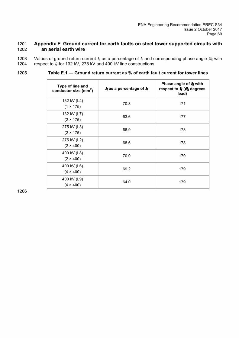
ENA Engineering Recommendation EREC S34 Issue 2 October 2017
Page 69
Appendix E Ground current for earth faults on steel tower supported circuits with 1201 an aerial earth wire 1202
Values of ground return current IE as a percentage of IF and corresponding phase angle ØE with 1203 respect to IF for 132 kV, 275 kV and 400 kV line constructions 1204
Table E.1 — Ground return current as % of earth fault current for tower lines 1205
Type of line and conductor size (mm2) IEas a percentage of IF
Phase angle of IE with respect to IF (ØE degrees
lead)
132 kV (L4) (1 × 175)
70.8 171
132 kV (L7) (2 × 175)
63.6 177
275 kV (L3) (2 × 175)
66.9 178
275 kV (L2) (2 × 400)
68.6 178
400 kV (L8) (2 × 400)
70.0 179
400 kV (L6) (4 × 400)
69.2 179
400 kV (L9) (4 × 400)
64.0 179
1206

ENA Engineering Recommendation EREC S34 Issue 2 October 2017 Page 70
Appendix F Typical values of resistance of long horizontal electrode 1207
1208
1209
Figure F.1 — Typical values of resistance of long horizontal electrode 1210 (taken from BS EN 50522) 1211
1212
30
20
15 12
10
6
4
2
1.5
1.2
1
0.8
0.6
0.5
0.4 0.35
0.3 0 0.2 0.4 0.6 0.8 1 1.2 1.4 1.6 1.8 2
Length (km)
R E
H (
Ω)

ENA Engineering Recommendation EREC S34 Issue 2 October 2017
Page 71
Appendix G Chain impedance of standard 132kV earthed tower lines 1213
Table G.1 gives chain impedances for a 132 kV L4 type construction with three towers/km and a 1214 “horse” earth wire (approx 70 mm2 aluminium ACSR, to BS 215-2:1970). 1215
Longitudinal impedance of earth wire is 0.443 + j 0.757 Ω/km (calculated using Carson-Clem 1216 formula [5]). 1217
The values assume more than 20 towers in series. 1218
Table G.1 — Chain impedance for 132 kV tower lines 1219
Footing resistance
(Ω)
Chain impedance ZCH (Ω) (complex notation)
Chain impedance ZCH (Ω) (angular notation)
1 0.543+j0.414 0.683Ð37.35
2 0.737+j0.52 0.902Ð35.21
3 0.886+j0.603 1.072Ð34.24
4 1.012+j0.674 1.215Ð33.7
5 1.122+j0.736 1.342Ð33.26
6 1.222+j0.793 1.457Ð32.96
7 1.314+j0.845 1.562Ð32.73
8 1.4+j0.893 1.661Ð32.55
9 1.48+j0.939 1.753Ð32.39
10 1.556+j0.982 1.841Ð32.26
15 1.89+j1.172 2.224Ð31.82
20 2.17+j1.333 2.547Ð31.55
25 2.42+j1.474 2.832Ð31.37
40 3.039+j1.83 3.547Ð31.05
1220
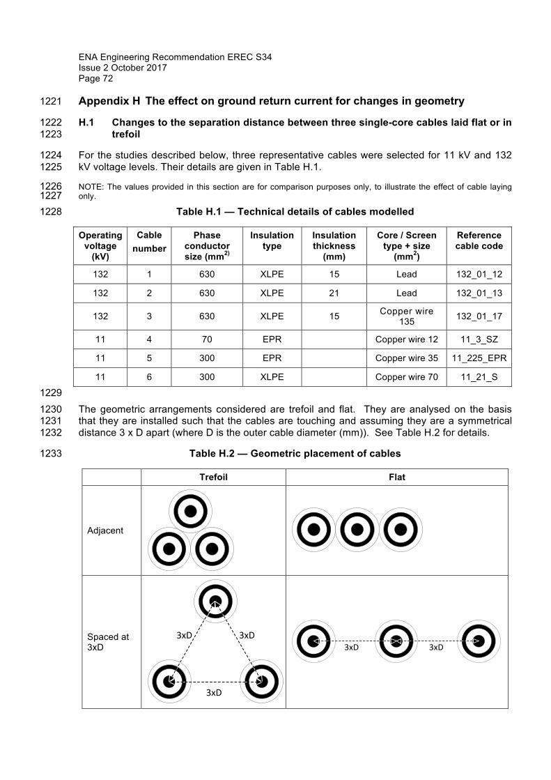
ENA Engineering Recommendation EREC S34 Issue 2 October 2017 Page 72
Appendix H The effect on ground return current for changes in geometry 1221
H.1 Changes to the separation distance between three single-core cables laid flat or in 1222 trefoil 1223
For the studies described below, three representative cables were selected for 11 kV and 132 1224 kV voltage levels. Their details are given in Table H.1. 1225
NOTE: The values provided in this section are for comparison purposes only, to illustrate the effect of cable laying 1226 only. 1227
Table H.1 — Technical details of cables modelled 1228
Operating voltage
(kV)
Cable number
Phase conductor size (mm2)
Insulation type
Insulation thickness
(mm)
Core / Screen type + size
(mm2)
Reference cable code
132 1 630 XLPE 15 Lead 132_01_12
132 2 630 XLPE 21 Lead 132_01_13
132 3 630 XLPE 15 Copper wire 135 132_01_17
11 4 70 EPR Copper wire 12 11_3_SZ
11 5 300 EPR Copper wire 35 11_225_EPR
11 6 300 XLPE Copper wire 70 11_21_S
1229 The geometric arrangements considered are trefoil and flat. They are analysed on the basis 1230 that they are installed such that the cables are touching and assuming they are a symmetrical 1231 distance 3 x D apart (where D is the outer cable diameter (mm)). See Table H.2 for details. 1232
Table H.2 — Geometric placement of cables 1233
Trefoil Flat
Adjacent
Spaced at 3xD
3xD
3xD
3xD3xD 3xD

ENA Engineering Recommendation EREC S34 Issue 2 October 2017
Page 73
IF
IEG
The 132kV cables were selected to show the difference that the sheath/screen configuration 1234 makes for the same size phase conductor. One standard cable contains a tubular conductor 1235 made of aluminium foil in addition to its stranded copper conductor. The cross-sectional view for 1236 this cable (trefoil format) is shown in Figure H.1. 1237
1238
Figure H.1 — Cross-sectional view for cable 3 1239
The circuit used to simulate the different cable arrangements and determine the effect on the 1240 earth return current is shown in Figure H.2. R1 and R2 are assumed nominal values of 0.5Ω. 1241
1242
Figure H.2 — Circuit used for analysis purposes 1243
Using the circuit described, studies were carried out for each of the cables of Table H.1 and the 1244 ground return current calculated for a set range of cable lengths. For each cable, four sets of 1245 studies were carried out, i.e. one for each physical arrangement of the individual cables shown 1246 in Table H.2. 1247
The results are shown in Figure H.3 and Figure H.4, with the ground return current 𝐼% shown as 1248 a percentage of the total earth fault current𝐼3. 1249
1
6
1
6 Z line - 1
Phase
representation of supply netw
ork
R 1 R 2 IE
IF

ENA Engineering Recommendation EREC S34 Issue 2 October 2017 Page 74
Cable 1: 630 mm2 with 15 mm XLPE, lead sheathed
1250
Cable 2: 630 mm2 with 21mm XLPE, lead sheathed
1251
Cable 3: 630 mm2 with 15 mm XLPE and composite screen/sheath (135 mm2 Cu and 45 mm2 Al)
Figure H.3 — Ground return current (IE) as a percentage of (IF) against circuit length for 1252
different 132 kV cable installation arrangements 1253
6789101112131415
0 2 4 6 8 10 12
I E/IF(%
)
Cable Length (km)
6789101112131415
0 2 4 6 8 10 12
I E/IF(%
)
Cable Length (km)
0
1
2
3
4
5
6
7
0 2 4 6 8 10 12
I E/IF(%
)
Cable Length (km)FLAT(3xD) TREFOIL(3xD) FLAT(Adjacent) TREFOIL(Adjacent)

ENA Engineering Recommendation EREC S34 Issue 2 October 2017
Page 75
Cable 4: (70 mm2 with 12 mm2 Cu screen)
1254
Cable 5: (300 mm2 with 35 mm2 Cu screen) 1255
Cable 6: (300 mm2 with 70 mm2 Cu screen)
Figure H.4 — Ground return current (IE) as a percentage of (IF) against circuit length for 1256
different 11 kV cable installation arrangements 1257
263034384246505458
0 2 4 6 8 10 12
I E/IF(%
)
Cable Length (km)
101214161820222426
0 2 4 6 8 10 12
I E/IF(%
)
Cable Length (km)
2
4
6
8
10
12
14
16
0 2 4 6 8 10 12
I E/IF(%
)
Cable Length (km)FLAT(3xD) TREFOIL(3xD) FLAT(Adjacent) TREFOIL(Adjacent)

ENA Engineering Recommendation EREC S34 Issue 2 October 2017 Page 76
The results show that earth return current increases when the distance between adjacent 1258 cables is increased. 1259
H.2 Conclusions 1260
From Figure H.3 and Figure H.4, the following can be deduced. 1261
Touching trefoil is the most effective arrangement in terms of minimising the ground return 1262 current. This is due to the more symmetrical arrangement and its impact on maximising mutual 1263 coupling effects. The ground return current increases in all cases in the following order: 1264
• touching trefoil. 1265
• touching flat. 1266 • 3 x D trefoil. 1267
• 3 x D flat. 1268 The difference between trefoil and flat arrangements can be disregarded for most studies. 1269
Other factors which influence the ground return current are: 1270
• The circuit length. 1271
• The electrical conductivity of the sheath/screen. This is illustrated when comparing the 1272 132 kV composite screen (copper and aluminium) against a similar cable with a higher 1273 impedance lead screen (cables 3 and 1). A similar effect can be seen between cables 5 1274 and 6. In the cables studied, the ground return current is approximately doubled for the 1275 cables with the higher impedance sheaths. The same effect is apparent with the 11 kV 1276 cables and cable 4 with its relatively small screen of 12 mm2/cable shows the importance of 1277 considering the screen size because the ground return current can reach almost 54% IF for 1278 this cable. 1279

ENA Engineering Recommendation EREC S34 Issue 2 October 2017
Page 77
Appendix I Transfer potential to distributed LV systems 1280
I.1 Background 1281
This issue relates to the transfer of voltage from HV systems to LV systems, when the LV 1282 system consists of multiple electrodes, as described in Section 5.4. 1283
I.2 Examples 1284
a) Equal LV electrode earth resistances 1285 It is useful to consider a worked example where assumed typical values have been used and 1286 the transfer voltage has been calculated. Figure I.1 shows the circuit together with the 1287 calculated parameters. 1288
1289
Figure I.1 — Example 1: Two electrodes of equal resistance1290
From Figure I.1, the surface potential experienced by electrodes A and B effectively act as 1291 voltage sources. Because electrodes A and B are connected together via an above ground 1292 conductor (assumed to have negligible resistance compared to the earth resistances) the 1293 potential difference of 100 V across the total series resistance of 20 Ω causes a current of 5A to 1294 circulate through the electrodes. This creates a voltage drop of 50 V across the earth resistance 1295 of A which is negative with respect to the local surface potential. This reduces the local 1296 electrode potential (by 50 V with respect to the local soil potential). Conversely at electrode B 1297 there is a 50 V drop across the earth resistance which increases the electrode potential by 50 V 1298 with respect to the local soil potential. The transfer potential on the combined LV electrode 1299 system is 150 V. 1300
This explains the changes in surface potential contours around combined LV electrodes. 1301
5 A
50 V 50V
LV Electrode A
VT= 150 V
VB= 100 V VA = 200 V
RB = 10 Ω RA= 10 Ω
LV Electrode B

ENA Engineering Recommendation EREC S34 Issue 2 October 2017 Page 78
b) Unequal LV electrode earth resistances 1302 Figure I.2 shows a similar example but where Electrode B has an earth resistance 5 times lower 1303 than Electrode A. 1304
1305
Figure I.2 — Example 2: Two electrodes of unequal resistance 1306
It can be seen that the potential on the combined LV electrode is much lower than the average 1307 value of 150 V. Because electrode B has a much lower resistance it has a smaller potential drop 1308 across it and so the combined electrode potential is closer to the potential on electrode B. 1309
c) More than two LV Electrodes 1310 A similar calculation process can be applied to combinations of more than two LV electrodes. 1311 The formula below gives the combined electrode potential for three electrodes, A, B & C. 1312
𝑉7 =𝑉C 𝑅D𝑅+ +𝑉D 𝑅C𝑅+ + 𝑉+ 𝑅C𝑅D
𝑅D𝑅+ + 𝑅C𝑅+ + 𝑅C𝑅D1313
The formula below allows a similar calculation to be made for four combined LV electrodes, A, B, 1314 C & D. 1315
𝑉7 =𝑉C 𝑅D𝑅+𝑅 +𝑉D 𝑅C𝑅+𝑅 + 𝑉+ 𝑅C𝑅D𝑅 + 𝑉 𝑅C𝑅D𝑅+
𝑅D𝑅+𝑅 + 𝑅C𝑅+𝑅 + 𝑅C𝑅D𝑅 + 𝑅C𝑅D𝑅+1316
Further formulae for more than four combined LV electrodes can easily be produced by 1317 continuing this pattern and would be best implemented via a computer programme subroutine 1318 loop. 1319
I.3 Discussion 1320
This method has been found to provide a conservative estimate of transfer potential to LV 1321 earthing systems when the HV earth resistance is reasonably accurate, ideally determined by 1322 measurement. If calculated, conservative results are obtained if the formula for the earth 1323 resistance of a hemispherical electrode is used. 1324
The above method may also be applied to a horizontal electrode which may be represented as 1325 a series of equally distributed vertical rods along its route. The coarsest representation is to 1326 model the horizontal electrode as two short vertical rods, the first at the point on the electrode 1327 nearest the HV electrode and the second at the furthest point. This method provides a 1328
8.3 A 8.3 A
16.7 V
LV Electrode A A
VT = 116.7 V
VB = 100 V VA = 200 V
RB= 2 Ω RA = 10 Ω
LV Electrode B

ENA Engineering Recommendation EREC S34 Issue 2 October 2017
Page 79
conservative estimate of the transfer potential to the LV electrode. The greater number of rods 1329 used to model the horizontal electrode, the more accurate the calculated transfer potential 1330 becomes. 1331
The method described above has been found to be reasonably accurate (and conservative) for 1332 soils with uniform resistivity and those where there is a lower resistivity deeper layer. Care 1333 should be taken when applying to soils where there is a high resistivity deeper layer, e.g. 1334 underlying rock, as transfer potentials may be underestimated and additional safety factors may 1335 need to be applied. 1336
Where there is a distributed HV electrode system, e.g. where there are extended HV cables 1337 with bare sheaths in contact with the soil, the accuracy of this approach will depend on the 1338 location of the LV electrodes relative to the HV electrode. The approach may be valid if the LV 1339 electrodes are in the opposite direction to the HV electrode otherwise the transfer potential will 1340 need to be calculated by more detailed methods. 1341
For detailed analysis of complex HV or LV electrode shapes and highly non-uniform soil 1342 resistivity structures, the use of computer simulation software will be required. 1343
I.4 Application to real systems 1344
The fact that the transfer potential is governed by the distance to the ‘centre of gravity’ of the LV 1345 electrode system from the HV electrode can help with the LV electrode design to minimise 1346 transfer potential. From this perspective, the best method is to install dominant parts of the LV 1347 electrode system as far as practicable from the HV electrode, i.e. towards the extremities of the 1348 LV system. 1349
I.5 Worked example: Pole-mounted 11 kV/LV substation 1350
A typical pole-mounted 11 kV substation arrangement is shown in Figure I.3. The HV and LV 1351 earthing systems are separated; in this example the transformer LV neutral/earth electrode is 1352 located 9 m away from the transformer HV earth electrode. A service cable provides an LV 1353 supply to a dwelling located 50 m away from the HV earth electrode and there is a LV PME 1354 earth electrode at the property. 1355
The HV earth electrode is assumed to be a 3.6 m earth rod of 16 mm diameter and the soil 1356 resistivity is assumed to be 75 Ωm. 1357
Using Formula R1, the HV electrode earth resistance is calculated to be 21.5 Ω. An earth fault 1358 current of 200 A is assumed to flow and is assumed to be disconnected in 1 s. The calculated 1359 EPR on the HV electrode is 4300 V. 1360
The surface potential 9 m away from the HV electrode can be calculated using Formula P6.2 as 1361 259V and would be experienced by LV earth electrode 1. In the absence of any additional LV 1362 earth electrodes, this voltage would be propagated through the LV neutral/earth conductor and 1363 may be experienced as a touch voltage by the dwelling occupants. This potential exceeds the 1364 permissible touch voltage for 1 s of 233 V and so would not be acceptable. 1365
Figure I.3 shows a second LV electrode (LV earth electrode 2) located at the dwelling that is 50 1366 m away from the HV electrode. Use of Formula P6.2 gives a calculated surface potential of 48 V 1367 that would be experienced by LV earth electrode 2. 1368

ENA Engineering Recommendation EREC S34 Issue 2 October 2017 Page 80
1369
1370
Figure I.3 — Example of pole-mounted 11 kV substation arrangement and LV supply to a 1371 dwelling 1372
Because LV earth electrodes 1 and 2 are connected via the LV neutral/earth conductor, and 1373 assuming they each have a similar earth resistance, the transfer potential on the LV earthing 1374 system (both electrodes and the interconnecting conductor) will be the average of the surface 1375 potential calculated at each LV electrode location, i.e. 154 V which is below the permissible 1376 touch voltage. 1377
If the resistance of LV earth electrode 2 was half that of LV earth electrode 1 the average 1378 potential will be weighted more towards the potential at LV earth electrode 2. From the formula 1379 in section 5.4.2, the combined potential on the LV earthing system would be (259 x1 + 48x2)/3 = 1380 118 V. 1381
This rather straightforward example illustrates how the electrode arrangement can be designed 1382 to significantly reduce the transfer potential. 1383
N/E L
N/E
HV EARTH ELECTRODE
LV EARTH ELECTRODE 1
LV EARTH ELECTRODE 2
9 m 41 m
L1 L2 L3

ENA Engineering Recommendation EREC S34 Issue 2 October 2017
Page 81
Bibliography 1384
Standards publications 1385
For dated references, only the edition cited applies. For undated references, the latest edition of 1386 the referenced document (including any amendments) applies. 1387
IEC 60287-3-1:2017, Electric cables – Calculation of the current rating – Part 3-1: Operating 1388 conditions – Site reference conditions 1389
IEC 60949:1988, Calculation of thermally permissible short-circuit currents, taking into account 1390 non-adiabatic heating effects 1391
PD IEC/TS 60479-1:2005+A1:2016, Effects of current on human beings and livestock. General 1392 aspects 1393
BS 215-2: 1970, Specification for aluminium conductors and aluminium conductors, steel-1394 reinforced for overhead power transmission. Aluminium conductors, steel-reinforced 1395
BS 7430:2011+A1:2015, Code of practice for protective earthing of electrical installations 1396
ENA EREC S36-1, Identification and Recording of Hot Sites - Joint Electricity / British Telecom 1397 Procedure 1398
IEEE 80, Guide for Safety in AC Substation Grounding 1399
Other publications 1400
[1] [M. Davies, T. Charlton, D. Baudin] New design methods to achieve greater safety in low 1401 voltage systems during a high voltage earth fault, CIRED Conference, Frankfurt, June 2011 1402
[2] [HSE] Reducing Risk Protecting People (R2P2) 1403
[3] [Sunde, E.D] Earth conduction effects in transmission systems, Dover Publications, 1967, 1404 pp75-79 1405
[4] [Schwarz S. J.] Analytical expression for resistance of grounding systems, AIEE 1406 Transactions on Power Apparatus and Systems, vol. 73, no. 13, part III-B, pp. 1011–1016, Aug. 1407 1954. 1408
[5] [Clem, J. E.], “Reactance of transmission lines with ground return,” AIEE Transactions on 1409 Power Apparatus and Systems, vol. PAS-50, pp. 901–918, Sept. 1931. 1410
Further reading 1411
SI 2002 no.2665, The Electricity Safety, Quality and Continuity Regulations 2002 (as amended) 1412
SI 2012 no. 381, The Electricity Safety, Quality and Continuity (Northern Ireland) Regulations 1413 2012 (as amended) 1414
ENA ETR 128, Risk assessment for BT operators working in a ROEP zone 1415
ENA ETR 129, ROEP risk assessment for third parties using equipment connected to BT lines 1416
1417