engineering optimization (an introduction with metaheuristic applications) || classic optimization...

CHAPTER 5

CLASSIC OPTIMIZATION METHODS II

The optimization methods we introduced in the last chapter are all well-established. In this chapter, we will continue to introduce more widely used, but relatively modern methods.

5.1 BFGS METHOD

The widely used BFGS method is an abbreviation of the Broydon-Fletcher-Goldfarb-Shanno method, and it is a quasi-Newton method for solving unconstrained nonlinear optimization. It is based on the basic idea of replacing the full Hessian matrix H by an approximate matrix B in terms of an iterative updating formula with rank-one matrices as its increment. Briefly speaking, a rank-one matrix is a matrix which can be written as r = ab where a and b are vectors, which has at most one non-zero eigenvalue and this eigenvalue can be calculated by b a.

To minimize a function f{x) with no constraint, the search direction sk at each iteration is determined by

Bksk = -Vf(xk), (5.1)

Engineering Optimization: An Introduction with Metaheuristic Applications. 85 By Xin-She Yang Copyright © 2010 John Wiley & Sons, Inc.

86 CHAPTER 5. CLASSIC OPTIMIZATION METHODS II

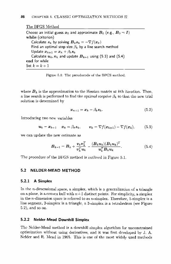
The BFGS Method Choose an initial guess 2:0 and approximate Bo (e.g., Bo = I) whi le (criterion)

Calculate Sk by solving BkSk = -Vf{xk) Find an optimal step size ßk by a line search method Update xk+i = Xk + ßkSk Calculate Uk,Vk and update Bk+\ using (5.3) and (5.4)

end for while Set k = k + 1

Figure 5.1: The pseudocode of the BFGS method.

where Bk is the approximation to the Hessian matrix at fcth iteration. Then, a line search is performed to find the optimal stepsize ßk so that the new trial solution is determined by

Xn+\ =Xk+ßkSk- (5.2)

Introducing two new variables

uk = Xk+i - Xk = ßkSk, vk = Vf{xk+i) - Vf(xk), (5.3)

we can update the new estimate as

R - R ■ V*Vk (BkUk)(BkUk)T

■öfc+i - Bk + — ψ— . (5.4) vj.Uk ul

kBkuk The procedure of the BFGS method is outlined in Figure 5.1.

5.2 NELDER-MEAD METHOD

5.2.1 A Simplex

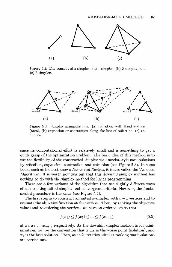
In the n-dimensional space, a simplex, which is a generalization of a triangle on a plane, is a convex hull with n + 1 distinct points. For simplicity, a simplex in the n-dimension space is referred to as n-simplex. Therefore, 1-simplex is a line segment, 2-simplex is a triangle, a 3-simplex is a tetrahedron (see Figure 5.2), and so on.

5.2.2 Nelder-Mead Downhill Simplex

The Nelder-Mead method is a downhill simplex algorithm for unconstrained optimization without using derivatives, and it was first developed by J. A. Neider and R. Mead in 1965. This is one of the most widely used methods

5.2 NELDER-MEAD METHOD 87

(a) (b) (c)

Figure 5.2: The concept of a simplex: (a) 1-simplex, (b) 2-simplex, and (c) 3-simplex.

'-ra+l Xn+1 > ^ Xn+1 * ^)

(a) (b) (c)

Figure 5.3: Simplex manipulations: (a) reflection with fixed volume (area), (b) expansion or contraction along the line of reflection, (c) reduction.

since its computat ional effort is relatively small and is something to get a quick grasp of the optimization problem. The basic idea of this method is to use the flexibility of the constructed simplex via amoeba-style manipulat ions by reflection, expansion, contraction and reduction (see Figure 5.3). In some books such as the best known Numerical Recipes, it is also called the 'Amoeba Algorithm'. It is worth pointing out tha t this downhill simplex method has nothing to do with the simplex method for linear programming.

There are a few variants of the algorithm tha t use slightly different ways of constructing initial simplex and convergence criteria. However, the fundamental procedure is the same (see Figure 5.4).

The first s tep is to construct an initial n-simplex with n + 1 vertices and to evaluate the objective function at the vertices. Then, by ranking the objective values and re-ordering the vertices, we have an ordered set so tha t

f(xi) < / (a*) < .- < f(xn+i), (5.5)

at X\,X2, ...,Xn+i, respectively. As the downhill simplex method is for minimization, we use the convention tha t xn+i is the worse point (solution), and x\ is the best solution. Then, at each iteration, similar ranking manipulat ions are carried out.


Then, we have to calculate the centroid x of simplex excluding the worst vertex xn+i

1 ™ x = - y ^ Χχ. (5.6)

n *—'

Using the centroid as the basis point, we try to find the reflection of the worse point xn+i by

xr = x + a(x — χη+ι), {θί > 0), (5.7)

though the typical value of a — 1 is often used. Whether the new trial solution is accepted or not and how to update the

new vertex, depends on the objective function at xr. There are three possibilities:

• If f{x\) < f(xr) < f(xn), then replace the worst vertex xn+i by xr, t ha t IS Xn+i ^ - Xr·

• If f(xr) < f(xi) which means the objective improves, we then seek a more bold move to see if we can improve the objective even further by moving/expanding the vertex further along the line of reflection to a new trial solution

xe = xr + β(χτ - x), (5.8)

where β = 2. Now we have to test if f{xe) improves even better. If f(xe) < f(xr), we accept it and update xn+i <— xe', otherwise, we can use the result of the reflection. That is xn+i <— xr.

• If there is no improvement or f(xr) > f(xn), we have to reduce the size of the simplex whiling maintaining the best sides. This is contraction

Xc = Xn+l +^f(x-Xn+l), (5.9)

where 0 < 7 < 1, though 7 = 1/2 is usually used. If f(xc) < f(xn+i) is true, we then update xn+\ <— xc.

If all the above steps fail, we should reduce the size of the simplex towards the best vertex x\. This is the reduction step

Xi = X\ + S(xi — xi), (i = 2,3, ...,n+ 1). (5.10)

Then, we go to the first step of the iteration process and start over again.

5.3 TRUST-REGION METHOD

The fundamental ideas of the trust-region have developed over many years with many seminal papers by a dozen of pioneers. A good history review of the trust-region methods can be found in the book by Conn, Gould and Toint (2000). Briefly speaking, the first important work was due to Levenberg

5.3 TRUST-REGION METHOD 89

Nelder-Mead (Downhill Simplex) Method

Initialize a simplex with n + 1 vertices in n dimension. while (stop criterion is not true) (1) Re-order the points such that f(xi) < f(x2) < ··· < f(xn+i)

with xi being the best and xn+i being the worse (highest value) (2) Find the centroid x using x = Σ7=ι χί/η excluding xn+\. (3) Generate a trial point via the reflection of the worse vertex

xr = x + a(x — xn+i) where a > 0 (typically a = 1) (a) if f(xi) < f(xr) < f(xn), xn+i <- xr\ end (b) if f(xr) < f(Xl),

Expand in the direction of reflection xe = xT + ß(xr — x) if f(xe) < f(xr), xn+i <— xe; else xn+1 <- xr; end

end (c) if f(xr) > f(xn), Contract by xc = xn+i + η(χ - χη+ι);

if f(xc) < f(xn+1), xn+1 <- xc; else Reduction by Xi= x\+8{xi — x\), (i = 2, ...,n+ 1); end

end end

Figure 5.4: Pseudocode of Nelder-Mead's downhill simplex method.

in 1944, which proposed the usage of addition of a multiple of the identity matrix to the Hessian matrix as a damping measure to stabilize the solution procedure for nonlinear least-squares problems. Later, Marquardt in 1963 independently pointed out the link between such damping in the Hessian and the reduction of the step size in a restricted region. Slightly later in 1966, Goldfelt, Quandt and Trotter essentially set the stage for trust-region methods by introducing an explicit updating formula for the maximum step size. Then, in 1970, Powell proved the global convergence for the trust-region method, though it is believed that the term 'trust region' was coined by Dennis in 1978, as earlier literature used various terminologies such as region of validity, confidence region, and restricted step method.

In the trust-region algorithm, a fundamental step is to approximate the nonlinear objective function by using truncated Taylor expansions, often the quadratic form

0fc(aj) « f(xk) + Vf(xk)Tu + -uTHku, (5.11)

in a so-called trust region Q,k defined by

ilk = {xe^\\T{x-xk)\\<^k}, (5.12)

where Ak is the trust-region radius. Here Hk is the local Hessian matrix. Γ is a diagonal scaling matrix that is related to the scalings of the optimization


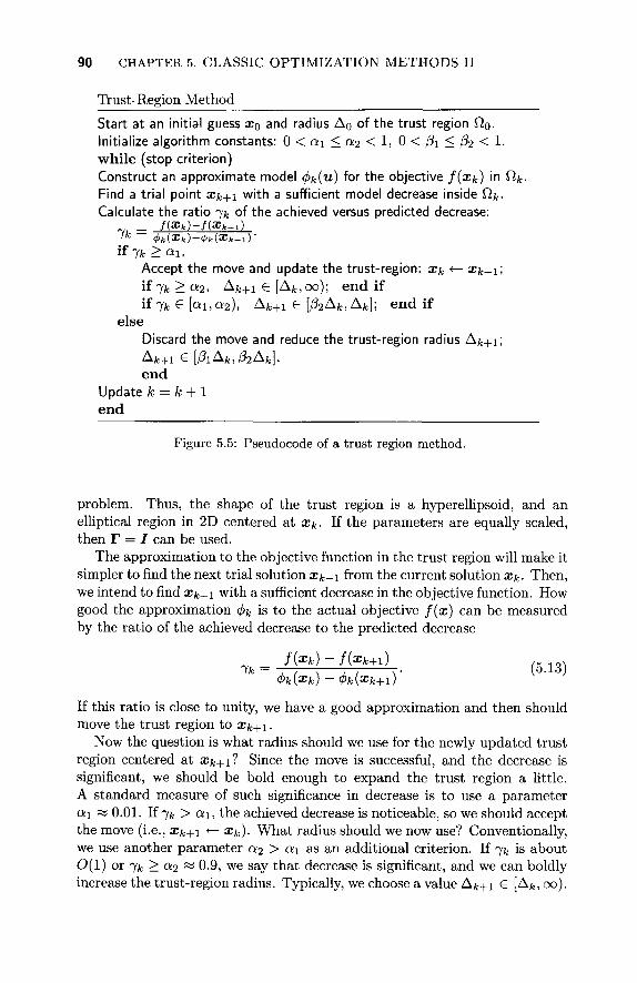
Trust-Region Method Start at an initial guess x0 and radius Δ 0 of the trust region Ωο· Initialize algorithm constants: 0 < a\ < a2 < 1, 0 < β\ < β2 < 1. wh i le (stop criterion) Construct an approximate model 4>k{u) for the objective f(xk) in ^k-Find a trial point Xk+i with a sufficient model decrease inside Ω^. Calculate the ratio jk of the achieved versus predicted decrease:

_ f(Xk)-f(Xk+i)

if 7fc > QI, Accept the move and update the trust-region: xk «— xk+i\ if Ik > a-2, Ak+i e [Δ*;,οο); end if if 7k e [αι,α2), Ak+1 G [ß2Ak,Ak]; end if

else Discard the move and reduce the trust-region radius Δ ^ + ι ; Afc+i e [ß1Ak,ß2Ak]. end

Update k = k + 1 end

Figure 5.5: Pseudocode of a trust region method.

problem. Thus, the shape of the trust region is a hyperellipsoid, and an elliptical region in 2D centered at xk. If the parameters are equally scaled, then T = I can be used.

The approximation to the objective function in the trust region will make it simpler to find the next trial solution xk+i from the current solution xk. Then, we intend to find xk+\ with a sufficient decrease in the objective function. How good the approximation φ\ί is to the actual objective f{x) can be measured by the ratio of the achieved decrease to the predicted decrease

7fc = / ( * * ) - / ( g f c + i ) , ( 5 1 3 ) 0fc(a;fc) -<t>k{xk+1)

If this ratio is close to unity, we have a good approximation and then should move the trust region to xk+\.

Now the question is what radius should we use for the newly updated trust region centered at xk+\l Since the move is successful, and the decrease is significant, we should be bold enough to expand the trust region a little. A standard measure of such significance in decrease is to use a parameter αι « 0.01. If 7fc > a\, the achieved decrease is noticeable, so we should accept the move (i.e., xk+\ <— xk). What radius should we now use? Conventionally, we use another parameter a2 > ot\ as an additional criterion. If ^k is about 0(1) or 7fe > Q2 « 0.9, we say that decrease is significant, and we can boldly increase the trust-region radius. Typically, we choose a value Δ^ + 1 G [Afc,oo).

5.4 SEQUENTIAL QUADRATIC PROGRAMMING 91

The actual choice may depend on the problem, though typically Δ^+ι « 2Δ^. If the decrease is noticeable but not so significant, that is αχ < jk < a2, we should shrink the trust region so that Δ^+ι £ [ß2Ak,Ak] or

ß2Ak < Ak+1 < Ak, (0 < ß2 < 1). (5.14)

Obviously, if the decrease is too small or *yk < ati, we should abandon the move as the approximation is not good enough over this larger region. We should seek a better approximation on a smaller region by reducing the trust-region radius

Ak+ie[ß1Ak,ß2Ak}, (5.15)

where 0 < ß\ < ß2 < 1, and typically ß\ = ß2 = 1/2, which means half the original size is used first.

To summarize, the typical values of the parameters are:

α ι = 0 . 0 1 , a 2 = 0 . 9 , β1=β2 = ±. (5.16)

5.4 SEQUENTIAL QUADRATIC PROGRAMMING

5.4.1 Quadratic Programming

A special type of nonlinear programming is quadratic programming whose objective function is a quadratic form

f(x) =-xTQx + bTx + c, (5.17)

where b and c are constant vectors. Q is a symmetric square matrix. The constraints can be incorporated using Lagrange multipliers and KKT formulation.

5.4.2 Sequential Quadratic Programming

Sequential (or successive) quadratic programming (SQP) represents one of the state-of-art and most popular methods for nonlinear constrained optimization. It is also one of the robust methods. For a general nonlinear optimization problem

minimize f(x), (5.18)

subject to hi(x) = 0 , (i = Ι,. , . ,ρ), (5.19)

&■(»)< 0, (j = l,...,q). (5.20)

The fundamental idea of sequential quadratic programming is to approximate the computationally extensive full Hessian matrix using a quasi-Newton updating method. Subsequently, this generates a subproblem of quadratic


programming (called QP subproblem) at each iteration, and the solution to this subproblem can be used to determine the search direction and next trial solution.

Using the Taylor expansions, the above problem can be approximated, at each iteration, as the following problem

minimize -sT\72L{xk)s + Vf(xk)Ts + f{xk), (5.21)

subject to Vhi(xk)Ts + hi(xk) — 0, (i = l,...,p), (5.22)

Vgjixkfs + gjixk) < 0, (j = l,...,q), (5.23)

where the Lagrange function, also called merit function, is defined by

v q L(x) = f(x) + ^2Xihi(x) + Y^ßj9j(x)

i = l j = l

= f{x) + \Th(x) + ßTg{x), (5.24)

where λ = (λι, . . . , λ ρ ) τ is the vector of Lagrange multipliers, and μ = (μι, . . . ,μ 9 ) τ is the vector of KKT multipliers. Here we have used the notation h = (hi{x),...,hp(x))T and g = (gi(x), ...,gq(x))T.

To approximate the Hessian V2L(xk) by a positive definite symmetric matrix iffc, the standard Broydon-Fletcher-Goldfarbo-Shanno (BFGS) approximation of the Hessian can be used, and we have

rr - u i VkV% HkukulHl H-k+i— jHfcH ψ ψτζ , (5.25)

vj.Uk u^HkUk where

uk = Xk+i - xk, (5.26) and

vk = VL(xk+1) - VL(xfc). (5.27)

The QP subproblem is solved to obtain the search direction

Xk+\ =xk + ask, (5.28)

using a line search method by minimizing a penalty function, also commonly called merit function,

p q

Φ(χ) = f(x) + ρ[Υ^\1Η(χ)\ +^2m&x{0,gj(x)}\, (5.29)

where p is the penalty parameter. It is worth pointing out that any SQP method requires a good choice of Hk

as the approximate Hessian of the Lagrangian L. Obviously, if Hk is exactly

EXERCISES 93

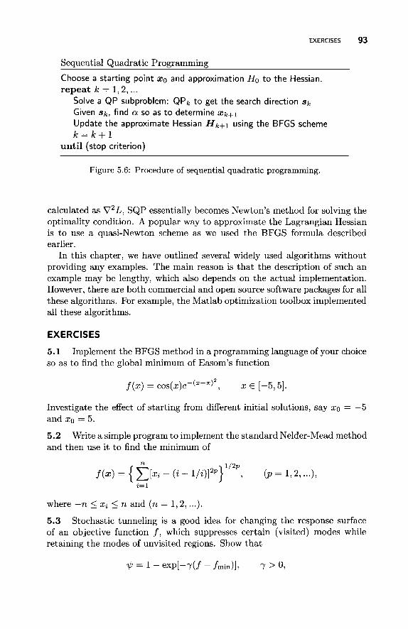
Sequential Quadratic Programming

Choose a starting point x0 and approximation H0 to the Hessian. repeat k — 1,2,...

Solve a QP subproblem: QPfc to get the search direction Sk Given Sk, find a so as to determine Xk+i Update the approximate Hessian Hk+i using the BFGS scheme k = k+l

until (stop criterion)

Figure 5.6: Procedure of sequential quadratic programming.

calculated as V2L, SQP essentially becomes Newton's method for solving the optimality condition. A popular way to approximate the Lagrangian Hessian is to use a quasi-Newton scheme as we used the BFGS formula described earlier.

In this chapter, we have outlined several widely used algorithms without providing any examples. The main reason is that the description of such an example may be lengthy, which also depends on the actual implementation. However, there are both commercial and open source software packages for all these algorithms. For example, the Matlab optimization toolbox implemented all these algorithms.

EXERCISES

5.1 Implement the BFGS method in a programming language of your choice so as to find the global minimum of Easom's function

f(x) = cos(x)e-{x-*)2, x <= [-5, 5].

Investigate the effect of starting from different initial solutions, say XQ = —5 and xo = 5.

5.2 Write a simple program to implement the standard Nelder-Mead method and then use it to find the minimum of

f(x) = { f > - (i - l/i)]2p}1/2P, (p = 1,2,...), i=\

where — n < Xi < n and (n = 1,2,...).

5.3 Stochastic tunneling is a good idea for changing the response surface of an objective function / , which suppresses certain (visited) modes while retaining the modes of unvisited regions. Show that

V>= 1 - e x p [ - 7 ( / - / m i n ) ] , 7 > 0 ,


preserves tha t the location of the global minimum. Here / m i n is the current minimum found so far during iterations, and 7 > 0 is a scaling factor which can be set 7 = 0 ( 1 / / ) .

REFERENCES

1. C. G. Broyden, "The convergence of a class of double-rank minimization algorithms", IMA J. Applied Math., 6, 76-90 (1970).

2. A. R. Conn, N. I. M. Gould, P. L. Toint, Trust-region methods, SIAM & MPS, 2000.

3. J. E. Dennis, "A brief introduction to quasi-Newton methods", in: Numerical Analysis: Proceedings of Symposia in Applied Mathematics (Eds G. H. Golub and J. Öliger, pp. 19-52 (1978).

4. A. V. Fiacco and G. P. McCormick, Nonlinear Porgramming: Sequential Un-constrained Minimization Techniques, John Wiley & Sons, 1969.

5. R. Fletcher, "A new approach to variable metric algorithms", Computer Jour-nal, 13 317-322 (1970).

6. D. Goldfarb, "A family of variable metric update derived by variational means", Mathematics of Computation, 24, 23-26 (1970).

7. S. M. Goldeldt, R. E. Quandt, and H. F. Trotter, "Maximization by quadratic hill-climbing", Econometrica, 34, 541-551, (1996).

8. N. Karmarkar, "A new polynomial-time algorithm for linear programming", Combinatorica, 4 (4), 373-395 (1984).

9. K. Levenberg, "A method for the solution of certain problems in least squares", Quart. J. Applied Math., 2, 164-168, (1944).

10. D. Marquardt, "An algorithm for least-squares estimation of nonlinear parameters", SIAM J. Applied Math., 11, 431-441 (1963).

11. J. A. Neider and R. Mead, "A simplex method for function optimization", Com-puter Journal, 7, 308-313 (1965).

12. M. J. D. Powell, "A new algorithm for unconstrained optimization", in: Non-linear Programming (Eds J. B. Rosen, O. L. Mangasarian, and K. Ritter), pp. 31-65 (1970).

13. D. F. Shanno, "Conditioning of quasi-Newton methods for function minimization", Mathematics of Computation, 25, 647-656 (1970).

engineering optimization (an introduction with metaheuristic applications) || classic optimization...

Documents