engineering optimization (an introduction with metaheuristic applications) || mathematical...

CHAPTER 3

MATHEMATICAL FOUNDATIONS

As this book is mainly about the introduction of engineering optimization and metaheuristic algorithms, we will assume that the readers have some basic knowledge of basic calculus and vectors. In this chapter, we will briefly review some relevant concepts that are frequently used in optimization.

3.1 UPPER AND LOWER BOUNDS

For a given non-empty set 5 £ S of real numbers, we now introduce some important concepts such as the supremum and infimum. A number U is called an upper bound for <S if x < U for all x € <S. An upper bound ß is said to be the least (or smallest) upper bound for S, or the supremum, if ß < U for any upper bound U. This is often written as

ß = supx Ξ supS = sup(<S). (3.1) xes

All such notations are widely used in the literature of mathematical analysis. On the other hand, a number L is called a lower bound for <S if x > L for

all x in S (that is Vx € S). A lower bound a is referred to as the greatest (or

Engineering Optimization: An Introduction with Metaheuristic Applications. 29 By Xin-She Yang Copyright © 2010 John Wiley & Sons, Inc.

30 CHAPTER 3. MATHEMATICAL FOUNDATIONS

largest) lower bound if a > L for any lower bound L, which is written as

a = super = inf <S = inf(<S). (3-2)

In general, both the supremum ß and the infimum a, if they exist, may or may not belong to S.

For example, any numbers greater than 5, say, 7.2 and 500 are an upper bound for the interval — 2 < x < 5 or [—2,5]. However, its smallest upper bound (or sup) is 5. Similarly, numbers such as -10 and —105 are lower bound of the interval, but —2 is the greatest lower bound (or inf). In addition, the interval S = [15, oo) has an infimum of 15 but it has no upper bound. That is to say, its supremum does not exist, or sup<S —► oo.

There is an important completeness axiom which says that if a non-empty set <S € 5ft of real numbers is bounded above, then it has a supremum. Similarly, if a non-empty set of real numbers is bounded below, then it has an infimum.

Both suprema and infima have the following properties:

inf(Q) = - s u p ( - Q ) , (3.3)

sup (p + q)= sup(P) + sup(Q), (3.4) peV,q€Q

sup(f(x)+g(x)) < snpf(x) + supg(x). (3.5)

Since the suprema or infima may not exist in the unbounded cases, it is necessary to extend the real numbers 5ft or

—oo < r < oo, (3.6)

to the affinely extended real numbers 5ft

5ft = 5ftU{±oo}. (3.7)

If we further define the sup(0) = —oo, for any sets of the affinely extended real numbers, the suprema and infima always exist if we let sup 5ft = oo and inf 5R = —oo.

Furthermore, the maximum for S is the largest value of all elements s S S, and often written as max(<S) or max<S, while the minimum, min(5) or min<S, is the smallest value among all s € S. For the same interval [—2,5], the maximum of this interval is 5 which is equal to its supremum, while its minimum 5 is also equal to its infimum. Though the supremum and infimum are not necessarily part of the set iS; however, the maximum and minimum (if they exist) always belong to the set.

However, the concepts of supremum (or infimum) and maximum (or minimum) are not the same, and maximum/minimum may not always exist.

3.2 BASIC CALCULUS 31

■ EXAMPLE 3.1

For example, the interval <S = [-2,7) or - 2 < x < 7 has the supremum of sup 5 = 7, but iS has no maximum. If any value a G <S is a maximum, then

a < b = —^ £ S, (3.8)

because b is the midpoint of a and 7. However, 7 is not part of <S. Therefore, the set S does not have a maximum. In addition, the set

sup{x e 5? : x7 < 7Γ} = \/π.

Similarly, the interval (—10,15] does not have a minimum, though its infimum is —10. Furthermore, the open interval (—2,7) has no maximum or minimum; however, its supremum is 7, and infimum is —2.

The maximum or minimum may not exist at all; however, we will assume they will always exist in many applications, especially in the discussion of optimization problems in this chapter. Now the objective becomes how to find the maximum or minimum in various optimization problems.

3.2 BASIC CALCULUS

For a univariate function f(x), its gradient or first derivative at any point P is defined as

ψ = ηχ)=^^ + Α?-^\ (3.9) dx v ' Δχ^ο Ax v ;

on the condition that such a limit exists. If the limit does not exist, we say that the function is not differentiable at this point P. For example, the simple absolute function |:r| is not differentiable at x = 0. Similarly, the differentiation of the gradient is the second derivative

ί δ ? = /"(*)· (3-10) Conventionally, the standard notation ^ is called Leibnitz's notation, while the prime notation is called Lagrange's notation. Newton's dot notation / = df/dt is now exclusively used for time derivative. We will use the prime notation ' and the standard notation df /dx interchangeably for convenience. Higher derivatives can be defined in a similar manner.

For differentiation, there are three important rules: the product rule, quotient rule, and chain rule. For a combined function f(x) = u(x)v(x), we have the product rule

f'{x) = [u{x)v{x)}' = u'{x)v(x) + u{x)v'{x). (3.11)


Similarly, if we replace v(x) by l/v(x) and using (l/v)' = -v'/v2, we have the quotient rule

u )/ = «W< ( 3 1 2 ) V V2

EXAMPLE 3.2

We can now use the above rules to carry out the following differentiation:

[sin(x) exp(x)]' = sin'(a;) exp(x) + sin(x)[exp(x)]'

= cos(x) exp(x) + sin(x) exp(x).

"sin(x)"|' sin'(a;) · x — sin(x) · (x)' xcosx — sin(x)

In case of a function f(x) can be written as a function of a simpler function f[u{x)\, we have the chain rule

(3.13) df(x) df du

dx du dx

■ EXAMPLE 3.3

Let us look at some simple examples.

[sin(x2)]' = cos(x2) · 2x = 2xcos(x2).

{exp[—sin(x2)]}' = exp[—sin(x2)] · [—cos(x2)] · 2x

= —2xcos(x2)exp[—sin(x2)].

[cos(x) exp(—x2)]' = — sin(x) exp(—x2) + cos(x) exp(—x2) · (—2a;)

= — sin(x) exp(—x2) — 2x cos(x) exp(—x2).

For functions with more than one independent variable, we have to use partial derivatives. For a bivariate function / (x , y), the partial derivatives are defined as

Ö^J/) n m f(x + *xty)-f(x,y) OX Ax->0,)/=fixed Δ χ

and dJ^A^f lim f(*,v + *v)-f{x,v) {315)

dy y Ay^O,x=&xed Ay providing that these limits exist. This is essentially equivalent to carrying out the standard differentiation for a univariate function while assuming other

3.2 BASIC CALCULUS 33

variables remaining constant. The total infinitesimal change df of a function due to the infinitesimal changes dx and dy can be written as

Higher partial derivatives can be defined in a similar manner, and we have

dx2 ~ dx^dx'' dy2 ~ dy^dy*' dxdy ~ dx^dy'' ( 3 ' 1 ? )

Since AxAy = AyAx, from the basic definition, we have

d2f d2f dxdy dydx

(3.18)

The differentiation rules still apply for partial derivatives. For multivariate functions with more than two independent variables, par

tial derivatives can be defined similarly.

■ EXAMPLE 3.4

The partial derivatives of f(x, y) = x2 + xy + sin(y2) are

- ^ = 2x + y, -rj-=x + cos(y2) -2y = x + 2y cos(y2),

d2f n d2f d r_ , o _ , 2. dx2 ' dxdy dx

[x + 2ycos{y2)] = l,

d2f d , 9 / . d ,„ . ,

d^l dy2

dydx dy dx dy

2 cos{y2) + 2y[- sin(y2)} · (2j/) = 2 cos(y2) - Ay2 sin(y2).

Q 2 f Q2 r

We can see that ßxßy — dydx ^ true indeed. Integration is basically a reverse process of differentiation, though it is much trickier. For example, from (xn)' = nxn~l, we have

l· ■ndx = —^—xn+1 + C, (3.19)

7 1 + 1

where C is an integration constant. This comes from the fact that the gradient of a function remains the same if a constant is added. In the special case n = — 1 for the integrand xn, this has to change to

/ x~1dx = lnx + C. (3.20)


When carrying out the differentiation of a definite integral with variable limits and the bivariate integrand, care should be taken. For example, we have

d fb{x) ., , . r„, ,db .. .da dx Ja(x)

f(x, y)dy = |/(x, b)— - f(x, a) dx. + Mx)

Ja{x)

df(x,y) dx dy. (3.21)

The Jacobian is an important concept concerning the change of variables and transformation. For a simple integral, the change of variables from x to a new variables u so that x = x(u), we have dx = (dx/du)du, which leads to

fXb fb dx / f{x)dx= f[x(u)]—du. (3.22)

This factor dx/du is in fact the Jacobian. For the change of variables in bivariate cases x = χ(ξ, η) and y = ·μ(ξ, η), we have the Jacobian J defined by

d(x,y) dx αξ dx dt]

dy αξ ay dr)

(3.23)

which is always a scalar or a simple value. The notation d(x, y)/d^, η) is just a useful shorthand commonly used in literature.

■ EXAMPLE 3.5

2

As an example, let us calculate the derivative of / sin(xy)dy with respect to x. We have

d_ dx ί

J X

sin(xy)dy = sin(x ■ x2) ■ (2x) — sin(a: · x) ■ 1 cos(xy) ■ ydy f J X

r2

= [2xsin(a;3) — sin(x2)] + / ycos(xy)dy. J X

To transform from a 2D Cartesian system (x, y) to polar coordinates (r, Θ), we have

x = rcos6, y = rsin9.

Therefore, the Jacobian is

j _ d{x,y) _ dx dr dx d9

dy dr »a de

dx dy dx dy lfr~dl)~~m~dr d(r,0)

cosö ■ rcos0 — (—rsinö) · sin# = r(cos2 Θ + sin2 Θ) = r.

3.3 OPTIMALITY 35

(a) (b)

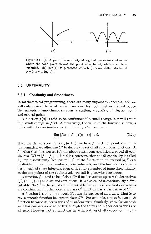
Figure 3.1: (a) A jump discontinuity at XQ, but piecewise continuous where the solid point means the point is included, while a circle is excluded, (b) |sin(a:)| is piecewise smooth (but not differentiable at a: = 0, ±π, ±2π,...).

3.3 OPTIMALITY

3.3.1 Continuity and Smoothness

In mathematical programming, there are many important concepts, and we will only review the most relevant ones in this book. Let us first introduce the concepts of smoothness, singularity, stationary condition, inflection point and critical points.

A function f(x) is said to be continuous if a small change in x will result in a small change in f(x). Alternatively, the value of the function is always finite with the continuity condition for any e > 0 at x — a

h m | / ( a + e) e—»Ό

■ / ( a - e ) l - O . (3.24)

If we use the notation f± for f(a ± e), we have /+ = /_ at point x = a. In mathematics, we often use C° to denote the set of all continuous functions. A function that does not satisfy the above continuous condition is called discontinuous. When |/_)_ — /_ | —» k > 0 is a constant, then the discontinuity is called a jump discontinuity (see Figure 3.1). If the function in an interval [a, b] can be divided into a finite number smaller intervals, and the function is continuous in each of these intervals, even with a finite number of jump discontinuity at the end points of the subintervals, we call it piecewise continuous.

A function / is said to be of class Cn if its derivatives up to ro-th derivatives (/'; /"> ···) / ^ ) all exist and continuous. It is also called n-continuously differ-entiably. So C1 is the set of all differentiable functions whose first derivatives are continuous. In other words, a class C1 function has a derivative of C°.

A function is said to be smooth if it has derivatives of all orders. That is to say, a smooth function belongs to class C°°. For example, exp(:r) is a smooth function because its derivatives of all orders exist. Similarly, x2 is also smooth as it has derivatives of all orders, though the third and higher derivatives are all zero. However, not all functions have derivatives of all orders. So in opti-


,

^ k 1 > 1

(b)

Figure 3.2: (a) \x\ is not differentiable at x = 0, (b) \jx has a singular point at x = 0.

mization, we often define a smooth function that has continuous derivatives up to some desired order over certain domains of interest. For this reason, we can loosely refer Cn functions as n-order smooth, though this is not a rigorous mathematical term. A curve f{x) in an interval [a, b] is called piece-wise smooth if it can be partitioned into a finite number of smaller 'pieces' or intervals, continuity holds cross the joins of the pieces and smoothness holds in each interval. In each interval, the function has a bounded first derivative that is continuous except at a finite number of points at the joints.

A singularity occurs if a function f(x) blows up or diverges or becomes unbounded. For example 1/x is singular at the point x = 0. We also call this singularity as a singular point (see Figure 3.2). In addition, as in each subdomain (—oo, 0) and (0, oo), |a;| is differentiable, and mathematically we call it piecewise differentiable.

3.3.2 Stationary Points

A stationary point of f(x) is a point x at which the stationary condition holds

f{x) = 0. (3.25)

We know that the first derivative is the gradient or the rate of change of the function. When the rate of change f'(x) is zero, we call it stationary. Consequently, such points are called stationary points. A smooth function can only achieve its maxima or minima at stationary points (and/or end points of an interval), so the stationary condition is a necessary condition for maxima or minima. However, being stationary is not sufficient to be maximal or minimal. In this further condition is needed. That is, if f"(x) > 0, the function f(x) achieves a local minimum at the stationary point. If f"(x) < 0, the stationary point corresponds to a local maximum.

3.3 OPTIMALITY 37

\J f">0

f"<0

Λ Figure 3.3: The sign of the second derivative at a stationary point, (a) f"(x) > 0, (b) f"(x) = 0, and (c) f"(x) < 0.

■ EXAMPLE 3.6

For a simple function f(x) = x2, the stationary condition f'(x) = 2x — 0 leads to x = 0 which is a stationary point. Since f"(x) = 2 > 0, / (0) = 0 is a local minimum. In fact, it is the only minimum in the whole domain (—00,00), and thus it is also the global minimum.

For f(x) = xe~x in the domain [0,00), its stationary condition becomes

f'(x) = e~x - xe~x = (1 - x)e~x = 0.

Since exp(—x) > 0, we have x = 1 as the stationary point. In addition, from f"(x) = (x - 2)e~x, we know that / " ( l ) = - e _ 1 < 0. So / m a x = e _ 1 at x = 1 reaches the maximum.

In the special case of f"(x) = 0, we have to use other methods such as the sign changes on both sides. The condition f"(x) = 0 determines a point of inflection, however, f'(x) is not necessarily zero. For example, f(x) = x3, the point x — 0 is an point of inflection, not an extremum (see Figure 3.3).

A point of a real function f(x) is called a critical point if its first derivative is zero or if it is not differentiable (see Figure 3.2). For example, |a;| at x = 0 is not differentiable, and thus it is a critical point. So a stationary point is a critical point, but a critical point may not be stationary. That is, critical points consists of stationary points and points at which the function is not differentiable (including singular points). In addition, a maximum or minimum can only occur at a critical point. For example, from Figure 3.2, we know that the global minimum of f(x) = \x\ is at x — 0, but this point is not stationary. However, x = 0 is a critical point as \x\ is not differentiable.

The stationary point of f(x) = sin(a;) is simply determined by

/ ' ( z ) = cos(a;) = 0,


Figure 3.4: Sine function sin(z) and its stationary points (marked with — and points of inflection (marked with o).

which leads t o i = ±π /2 , ±3π/2, . . . which are marked with ' - ' in Figure 3.4. The points of inflection are determined by

f"{x) = - sin(x) = 0.

That is x = 0, ±π, ±2π,... which are marked with o in the same figure.

3.3.3 Optimality Criteria

Now we can introduce more related concepts: feasible solutions, the strong local maximum and weak local maximum.

A point x that satisfies all the constraints is called a feasible point and thus is a feasible solution to the problem. The set of all feasible points is called the feasible region. A point cc* is called a strong local maximum of the nonlinearly constrained optimization problem if f(x) is defined in a δ-neigbourhood Ν(χ*,δ) and satisfies f(x*) > f(u) for Vtt € Ν(χ*,δ) where δ > 0 and u φ χ*. If a:* is not a strong local maximum, the inclusion of equality in the condition f(x*) > f(u) for V« G -/V(cc*, δ) defines the point x* as a weak local maximum (see Figure 3.5). The local minima can be defined in the similar manner when > and > are replaced by < and <, respectively.

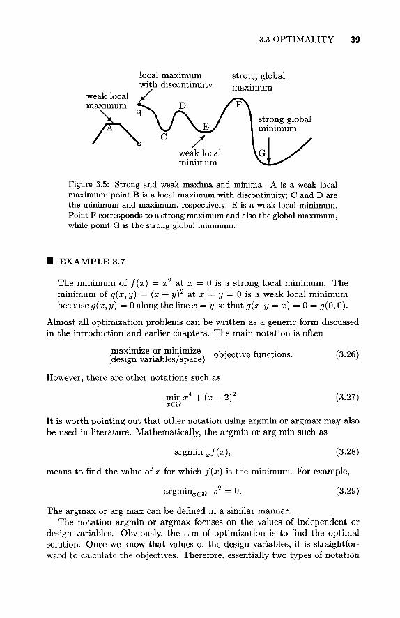
Figure 3.5 shows various local maxima and minima. Segment A is a weak local maximum, while point B is a local maximum with a jump discontinuity. C and D are the local minimum and maximum, respectively. Region E has a weak local minimum because there are many (well, infinite) different values of x which will lead to the same value of f(x*)- Point F is the global maximum which is also a strong maximum. Finally, G is the strong global minimum. However, at point B, there exists a discontinuity, and f'{x) is not defined unless we are only concerned with the special case of approaching from the right. We will not deal with this type of minima or maxima in detail. In our present discussion, we will assume that both f(x) and f'(x) are always continuous or f(x) is everywhere twice-continuously differentiable. In a more general case, we will assume that all objective functions belong to class C°.

3.3 OPTIMALITY 39

local maximum with discontinuity

strong global maximum

weak local maximum

strong global minimum

weak local minimum

Figure 3.5: Strong and weak maxima and minima. A is a weak local maximum; point B is a local maximum with discontinuity; C and D are the minimum and maximum, respectively. E is a weak local minimum. Point F corresponds to a strong maximum and also the global maximum, while point G is the strong global minimum.

■ EXAMPLE 3.7

The minimum of f(x) = x2 at x = 0 is a strong local minimum. The minimum of g(x, y) = (x — y)2 at x = y = 0 is a weak local minimum because g(x, y) = 0 along the line x = y so that g(x, y = x) = 0 = <?(0,0).

Almost all optimization problems can be written as a generic form discussed in the introduction and earlier chapters. The main notation is often

iiuuuuiizK wi miuimize objective functions.

(design variables/space) J

However, there are other notations such as min:r4 + ( a ; -2 ) 2 .

(3.26)

(3.27)

It is worth pointing out that other notation using argmin or argmax may also be used in literature. Mathematically, the argmin or arg min such as

argmin xf(x), (3.28)

means to find the value of x for which f(x) is the minimum. For example,

argminxe5R x2 = 0. (3.29)

The argmax or arg max can be defined in a similar manner. The notation argmin or argmax focuses on the values of independent or

design variables. Obviously, the aim of optimization is to find the optimal solution. Once we know that values of the design variables, it is straightforward to calculate the objectives. Therefore, essentially two types of notation


are the same. Conventionally, the optimization notation using 'min' or 'max' is just a shorthand, and it emphasize the fact that we intend to minimize or maximize certain objectives or targets.

In general, the maximum or minimum of a function can only occur at the following places:

• A stationary point determined by f'(x) = 0;

• A critical point when the function is not differentiable;

• At the boundaries.

3.4 VECTOR AND MATRIX NORMS

For a vector with n components (or simply an n-vector)

υ = (vi v2 ... vn) =

\vnJ its p-norm or £p-norm is denoted by | |Ü|L and defined as

n -. i

ΙΗΡ = ( Σ Μ Ρ ) Ρ' <3·31) » = 1

where p is a positive integer. From this definition, it is straightforward to show that the p-norm satisfies the following conditions: ||u|| > 0 for all v, and ||t?|| = 0 if and only if v = 0. This is the non-negativeness condition. In addition, for any real number a, we have the scaling condition: ||α«|| = α||ι;||.

The three most common norms are one-, two- and infinity-norms (or l\, £%, ioo) when p = 1,2, and oo, respectively. For p = 1, the one-norm is just the simple sum of the absolute value of each component \vi\, while the £2-norm ||«||2 for p = 2 is the standard Euclidean norm because ||v||2 is the length of the vector v

V2 (3.30)

\\v\\2 = V^T:v=\Jv21+vi + ...+vl (3.32)

where the notation u ■ v is the inner product of two vectors u and v. The inner product of two vectors is defined as

n

U- V =<U,V >= UTV = 2_\UiVi- (3.33) 8 = 1

Therefore, the Euclidean norm or ^2-norm of v is the square root of its inner product. That is

= Vv¥v = (v21 + ... + v2

n)1^. (3.34)

3.4 VECTOR AND MATRIX NORMS 41

The norms and inner product satisfy the following Cauchy-Schwartz inequality

\uTv\ < \\u\\2 H | 2 . (3.35)

The £i-norm is in fact the sum-absolute value and is given by

IMIi = l^il + M + ... + k | . (3.36)

For the special case p = oo, the ^Όο-norm is also called the Chebyshev norm. We denote «max as the maximum absolute value of all the components Vi, or

IMIoo = B m H = max|ui| =max( | i ; i | , | ? ;2 | , . . . ,k | ) . (3.37)

i=l i=l

= l i m « a x ) £ ( £ | - ^ n i = t , m a x l i m ^ l - ^ - n i . (3.38) l=\ 1 = 1

Since \vi/vmaK\ < 1 and for all terms |vi/vmaX| < 1, we have

| ^ i / W m a x | P ->· 0 , f o r p -»■ OO.

Thus, the only non-zero term in the sum is the one with \vi/vmax\ = 1, which means that

lim V K A w | p = 1. (3.39) p—KX> z—'

i=l

Therefore, we finally have

IMIoo = t ;max = max|vi|. (3.40)

For the uniqueness and consistency of norms, it is necessary for the norms to satisfy the triangle inequality

||u + t > | | < M + IM|. (3.41)

It is straightforward to check that this is true for p = 1,2, and oo from their definitions. The equality occurs when u = v. It remains as an exercise to verify this inequality for any p > 0.

■ EXAMPLE 3.8

For two 4-dimensional vectors

u = ( 5 2 3 - 2 ) T , « = ( - 2 0 1 2) T ,

then the p-norms of u are

lltilN =151+ 121+ 131+ 1-21 = 12,


u y/52 + 22 + 32 + ( -2)2 = v/42,

and ||u||00 = max(5,2,3,-2) = 5.

Similarly, H«^ = 5, ||«||2 = 3 and H « ^ = 2. We know that

u-\- v

/ 5 + ( - 2 ) \ 2 + 0 3 + 1

V-2 + 2 /

/ 3 \ 2 4

and its corresponding norms are ||u + w||j = 9, ||u + «||2 ||u + ii||00 = 4. It is straightforward to check that

||« + ü | | 1 = 9 < 1 2 + 5 = | H | 1 + ||«||1,

II« + t>||2 = Vw < V42 + 3 - ||u||2 + ||«||2,

29 and

and ||u + «|| 4 < 5 + 4 = ||it||

Matrices are the extension of vectors, so we can define the corresponding norms. For an m x n matrix A = [Oy], a simple way to extend the norms is to use the fact that Au is a vector for any vector ||u|| = 1. So the p-norm is defined as

m n

ΜΙΙΡ = ( Σ Σ Ι ^ Π 1 / Ρ - (3·42) i = l j=l

Alternatively, we can consider that all the elements or entries α̂ - form a vector. A popular norm, called Frobenius form (also called the Hilbert-Schmidt norm), is defined as

m n

ι ^ = (ΣΣ4) 1/2

(3.43) i= l j=\

In fact, Frobenius norm is a 2-norm. Other popular norms are based on the absolute column sum or row sum.

For example,

1 < 7 < η Α—' 1<J l=L

which is the maximum of absolute column sum, while

(3.44)

K i < m *—^ (3.45)

3.5 EIGENVALUES AND DEFINITENESS 43

is the maximum of the absolute row sum. The max norm is defined as

II^ILax = m a x { M } · (3-46)

From the definitions of these norms, we know that they satisfy the non-negativeness condition ||A|| > 0, the scaling condition ||aA|| = |a|||.A||, and the triangle inequality ||A + B | | < ||A|| + | |B| | .

■ EXAMPLE 3.9

For the matrix A =

\\Α\\ν =

, we know that

\2 = y/22 + 32 + 42 + ( -5) 2 = >/54,

121 + 131 l^lloo = m a x

|4| + and \\A\\max = 5.

3.5 EIGENVALUES AND DEFINITENESS

3.5.1 Eigenvalues

The eigenvalues λ of an n x n square matrix A are determined by

Au = Xu, (3.47)

or (A - XI)u = 0.

Any non-trivial solution requires that

det \A - XI\ = 0,

(3.48)

(3.49)

which is often referred to as the characteristic equation. We can also write it as

o n — λ αΐ2 ■■· ciin 0-21 0-11 — X ■■■ 0,2η

ο, (3.50)

O-nl αη2 ■■■ αηη ~ X

which again can be written as a characteristic polynomial

λη + α , , - ιλ"- 1 + ... + α0 = (λ - Ai)fcl...(A - ΧΡΡ = 0, (3.51)


where Aj are the eigenvalues that could be complex numbers. kp is the multiplicity of the eigenvalue \p, and ki + k2 + ... + kp = n. For each eigenvalue λ, there is a corresponding eigenvector u whose direction can be determined uniquely. However, the length of the eigenvector is not unique because any non-zero multiple of u will also satisfy equation (3.47), and thus can be considered as an eigenvector. For this reason, it is usually necessary to apply an additional condition by setting the length as unity, and subsequently the eigenvector becomes a unit eigenvector.

In general, a real n x n matrix A has n eigenvalues Xi(i = 1,2, ...,n); however, these eigenvalues are not necessarily distinct. If the real matrix is symmetric, that is to say A = A, then the matrix has n distinct eigenvectors, and all the eigenvalues are real numbers. The eigenvalues of an inverse A" are the reciprocals of the eigenvalues of A.

Eigenvalues have the interesting connections with the matrix,

tr(A) = ̂ 2aü = λι+λ2 + ... + Xn.

In addition, we also have

det(A) = Y[Xt.

(3.52)

(3.53)

For a symmetric square matrix, the two eigenvectors for two distinct eigenvalues Xi and Xj are orthogonal ujUj — 0.

■ EXAMPLE 3.10

The eigenvalues of the square matrix

'4 9 A = 2 - 3 Γ

can be obtained by solving

4 - λ 9 2 - 3 - λ 0.

We have (4 - A)(-3 - λ) - 18 = (A - 6)(A + 5) = 0.

Thus, the eigenvalues are A = 6 and A = —5. Let v = (v\ v2)T be the eigenvector, we have for A = 6

\A-\I\

which means that

-2vx + 9v2 = 0, 2vx - 9v2 = 0.

- 2 9 \ (νχ 2 -9 I U 0,


These two equations are virtually the same (not linearly independent), so the solution is

9 V! = r , .

Any vector parallel to v is also an eigenvector. In order to get a unique eigenvector, we have to impose an extra requirement, that is, the length of the vector is unity. We now have

or

which gives V2 = ±2/v/85, and vi = ±9/\/85· As these two vectors are in opposite directions, we can choose either of the two directions. So the eigenvector for the eigenvalue λ = 6 is

Similarly, the corresponding eigenvector for the eigenvalue λ = —5 is „ = ( - Ϊ / 2 / 2 V^/1)T.

Furthermore, we know the trace of A is t r (A)= 4 + (—3) = 1, while its determinant is det A = 4 x (—3) — 2 x 9 = —30. Prom its eigenvalues 6 and —5, we have indeed

2

tr(A) = l = 5^Ai = 6 + (-5), i = l

and 2

detA = J J A , = 6X (-5) = -30. i = l

We know that the inverse of A is

3 - 9 \ _ A / 1 0 3/10 λ 4 x ( - 3 ) - 2 x 9 ^ - 2 4 ; ^1/15 - 4 / 3 0 /

The eigenvalues of A~ are

A = 1/6 , -1 /5 ,

which are exactly the reciprocals of the eigenvalues λ = 6 and —5 of the original matrix A. That is A = 1/λ.


3.5.2 Definiteness

A square symmetric matrix A (i.e., AT = A) is said to be positive definite if all its eigenvalues are strictly positive (A, > 0 where i = 1,2, ...,n). By multiplying (3.47) by uT, we have

uT Au = uT\u = XuTu, (3.54)

which leads to uTAu

This means that uTAu > 0, if λ > 0.

In fact, for any vector v, the following relationship holds

vTAv > 0. (3.57)

For v can be a unit vector; thus all the diagonal elements of A should be strictly positive as well. If the equal sign is included in the definition, we have semi-definiteness. That is, A is called positive semidefinite if uTAu > 0, and negative semidefinite if uTAu < 0 for all u.

If all the eigenvalues are non-negative or Aj > 0, then the matrix is called positive semi-definite. If all the eigenvalues are non-positive or A; < 0, then the matrix is called negative semi-definite. In general, an indefinite matrix can have both positive and negative eigenvalues. Furthermore, the inverse of a positive definite matrix is also positive definite. For a linear system Au = f, if A is positive definite, the system can be solved more efficiently by matrix decomposition methods.

■ EXAMPLE 3.11

In order to determine the definiteness of a 2 x 2 symmetric matrix A

we first have to determine its eigenvalues. From \A — XI\ = 0, we have

^(α~βχ

aß_x) = (*-x?-f = o,

or A = a ± ß.

Their corresponding eigenvectors are

(3.55)

(3.56)


Eigenvectors associated with distinct eigenvalues of a symmetric square matrix are orthogonal. Indeed, they are orthogonal since we have

( 1 l ^ \ 1 1 1 - 1

The matrix A will be positive definite if

α±β>0,

which means a > 0 and a > max(+/3, —/?). The inverse

A~l 1 ( a -0 a2 - ß2 \-ß a

will also be positive definite. For example,

A=[ I " A B iW 9 - 2 3 / ' V 9 10

are positive definite, while

D 2 3 3 2

is indefinite.

For a symmetric matrix, it may be easier to test its definiteness using determinants of principal minor matrices, rather than calculating the eigenvalues. The ith. principal minor A^1' of an n x n square matrix A = [ay] is formed by the first i rows and i columns of A. That is

AW = («.„), A < a > = ( ; " ; i 2 Y A^=[a21 a22 a23), ..., (3.58) \a2i a22J \ I v 7 \a3i a32 a33/

whose determinants can be used to verify the definiteness. If all the determinants of its principal minors A^\...,A^ are strictly positive, then A is positive definite. If all the determinants are all nonnegative, then A is positive semidefinite. On the other hand, if the determinants alternate in signs with det(A^) < 0 (or < 0), then A is negative (semi)definite.

■ EXAMPLE 3.12

For example, for a symmetric real matrix

'a ß A — 'β ΊΓ


we have its principal minors

For A to be positive definite, it requires that

det(A(1)) = a > 0, det(A(2)) = a 7 - β2 > 0.

For example, if / 802 -400\

~ V-400 200 ) ' we have a = 802, /3 = -400 and 7 = 200. Since 802 > 0 and a-y - β2 = 400 > 0. So it is positive definite. We will use this result later in this chapter.

3.6 LINEAR AND AFFINE FUNCTIONS

3.6.1 Linear Functions

Generally speaking, a function is a mapping from the independent variables or inputs to a dependent variable or variables/outputs. For example, f(x, y) = x2 + y2 + xy is a function which depends on two independent variables. This function maps the domain SR2 (for —00 < x < 00 and —00 < y < 00) to / on the real axis as its range. So we use the notation / : Si2 —> 5R to denote this. In general, a function f(x,y,z,...) will map n independent variables to m dependent variables, and we use the notation / : 3ϊη —► 5Rm to mean that the domain of the function is a subset of W1 while its range is a subset of 5Rm. The domain of a function is sometimes denoted by dom(/) or dom / .

The inputs or independent variables can often be written as a vector. For simplicity, we often use a vector x = (x,y,z, ...)T for multiple variables. Therefore, f{x) is often used to mean f(x,y,z,...) or f(xi,X2, ■■■,Xn)·

A function C(x) is called linear if it satisfies

C(x + y) = C(x)+C(y), C(ax) = aC(x), (3.59)

for any vectors x and y, and any scalar agSR.

■ EXAMPLE 3.13

To see if f(x) = /(ιτι,α^) = 2xi + 3x2 is linear, we use

/ ( z i +2/1,^2+2/2) =2(xi +2/1) +3(2:2+2/2) = 2xi +2yi + 3x2 + 3y2

= [2xi + 3x2] + [2yi + 3y2] = f{xi, x2) + f{yi,yi).

3.6 LINEAR AND AFFINE FUNCTIONS 49

In addition, for any scalar a, we have

f(ax\,ax2) = 2ax\ + 3ax2 = α[2χχ + 3x2] = af{x\,x2).

Therefore, this function is indeed linear. This function can also be written as a vector form

f{x) = (2 3) Q = ax = aTu,

where a — (2 3)T and x = [x\ x2)T.

3.6.2 Affine Functions

A function F is called affine if there exists a linear function C : ϊϊ™ —► 5Rm

and a vector constant c such that

F = C{x) + c. (3.60)

In general, an affine function is a linear function with a translation, which can be written as a matrix form

F = Ax + c, (3.61)

where A is an m x n matrix, and c is a column vector in 3?".

■ EXAMPLE 3.14

The function 5x + 5

-2x + 3y + 2

is affine because it can be written as

*=(Λ ?)(;)♦(; Indeed, it is a linear function.

3.6.3 Quadratic Form

Quadratic forms are widely used in optimization, especially in convex optimization and engineering optimization. Loosely speaking, a quadratic form is homogenous polynomial of degree 2 of n variables. For example, 3x2 + 10xy + 7y2 is a binary quadratic form, while x2 + 2xy + y2 — y is not.


For a real nxn symmetric matrix A and an n-vector u, their combination

Q = uTAu, (3.62)

is called a quadratic form. Since A — [α^], we have

n n n n

Q = u Au = VJ 2_] Uidijiij = 2_. / . lijUiUj i = l j = l i = l j = l

n n 2 — 1

= ^2 aHui + 2 5 3 Σ / aijUiUj. (3.63) i = l i=2 j = l

■ EXAMPLE 3.15

(1 2 \ T

I and it = (ui «2) , we have

uTAu=(Ul u2)(^ f)(fy

( u\ + 2u2 \ = 3iii + 10«iii2 + 7u2.

2ui + 5u2J

In fact, for a binary quadratic form Q{x, y) = ax2 + bxy + cy2, we have

(x y)(^ ^(^=(α + β)χ2 + (α + 2β + Ί)χυ + (β + Ί)ν2.

If this is equivalent to Q(x, y), it requires that α + β = α, α + 2/3 + 7 = 6, β + Ί = €,

which leads to a + c = b. This means that not all arbitrary quadratic functions Q(x,y) are quadratic form.

If A is real symmetric, its eigenvalues Xi are real and its eigenvectors Vi are orthogonal. Therefore, we can write u using eigenvector basis and we have

n

u = Yjaivi. (3.64)

In addition, A becomes diagonal in this basis. That is

A=\ ·.. . (3.65) K

3.7 GRADIENT AND HESSIAN MATRICES 51

Subsequently, we have n n

Au = ^2 aiAvi = X ] k&iVi, (3.66)

which means that n n n

uTAu = ^2 Σ ^ictjaivjvi = ^ λ*α?> (3.67) j = l i = l i = l

where we have used the fact that vfvi = 1.

3.7 GRADIENT AND HESSIAN MATRICES

3.7.1 Gradient

The gradient vector of a multivariate function f{x) is defined as a column vector

G ( * ) = V / ( * ) E E ( £ £ , & . ■■■■&)Γ . (3.68)

where x = (xi,X2,...,xn)T is a vector. As the gradient V / (x ) of a linear function f(x) is always a constant vector k, then any linear function can be written as

f(x) = kTx + b, (3.69)

where b is a vector constant.

3.7.2 Hessian

The second derivatives of a generic function f(x) form a n n x n matrix, called Hessian matrix, given by

H(x) = S72f{x)

/ 9V d2f \ I lh% "· dxidx„ \

\ 92f ±L· I \dxndxi ' ' ' dx-n '

(3.70)

£)2 f Q2 f

which is symmetric due to the fact that dx.gx. = QX.QX. ■ When the Hessian matrix H{x) = A is a constant matrix (the values of its entries are independent of x), the function f(x) is called a quadratic function, and can subsequently be written as the following generic form

f(x) = ]-xTAx + kTx + b. (3.71)

The use of the factor 1/2 in the expression is to avoid the appearance of a factor 2 everywhere in the derivatives, and this choice is purely for convenience.


EXAMPLE 3.16

The gradient of f(x, y,z) = xy -y exp(-z) + z cos(a;) is simply

G = (y — z sin x x — e

The Hessian matrix is / ePf d2f a2f \

ye

H

dx2 dxdy dxdz

— 2-1 dx dy2

a2f dzdx dzdy dz2

I-

V-si sin a;

cos x

z cos x 1 — sin x\

1 0 e~z

-ye ZJ

3.7.3 Function approximations

In many optimization problems, we have to use some form of estimations to approximate the objective function, and this is often based on the Taylor expansion

f(x) = f(x0)+f'(x0)(x-xo)+ /"(so) 2!

f(n) {x-x0y+...+ J—r(x-x0)n+..., (3.72) n!

where xo is a known point around which the approximation is made. This uni-variate form can be extended to functions of multiple variables using vectors, and we have

f{x) = f(x0) + Vf(x0)T(x - xo) + i ( x - x 0 ) T ( V 2 / ) ( * - xo) + ···, (3-73)

where we can see that the second term involving the gradient V / and the third term involving the Hessian matrix V 2 / . Here we have used a short-hand notation V / T to mean (V/(a;o))T, and this notation is very commonly used in optimization. As f(xo) is known and V / is small near an optimal point, the third term is a quadratic form which dominates the whole expansions.

3.7.4 Optimality of multivariate functions

Similar to the univariate case, the optima of a multivarate function can only occur at three places: a stationary point where the gradient vector is zero, a non-differentiable point, and the boundary. For both non-differentiable point and boundary, we have to deal with them separately, often depending on each individual case.

For the case of stationary points, the maximum or minimum of a multivariate function f(x) = f(xi, ...,xn) requires

G = Vf(x) = 0. (3.74)

3.8 CONVEXITY 53

That is df ^ - = 0 , (i = l ,2, . . . ,n) , (3.75)

which leads to a stationary point x*. Whether the point x* is maximum or minimum is determined by the denniteness of its Hessian matrix. It is a local minimum if i / (x*) is positive definite, and a local maximum if JJ(x*) is negative definite. This extension is similar to the case for univariate functions. However, if H(x*) is indefinite, it may be a saddle point. For example, f(x, y) = xy has a saddle point at (0,0).

■ EXAMPLE 3.17

For the banana function f(x,y) = (x — l ) 2 + 100(y - x2)2, its gradient and Hessian can be written as

G - v / - ( v 20%-*») J - 0 '

„ _ (2 + 1200a;2 - 400?/ -400tt\ V -400u 200 J'

From G = 0, we have

2{x - 1) - 400*(iy - x2) = 0, 200{y - x2) = 0.

This means that ** = 1 and y* = 1. The Hessian matrix at this point becomes

^ ί 1 · 1 ) - ^-400 200 J '

We know from an earlier example (see Example 3.12), it is positive definite. Therefore, the point (1,1) is a minimum.

3.8 CONVEXITY

3.8.1 Convex Set

Knowing the properties of a function can be useful for finding the maximum or minimum of the function. In fact, in mathematical optimization, nonlinear problems are often classified according to the convexity of the defining function(s). Geometrically speaking, an object is convex if for any two points within the object, every point on the straight line segment joining them is also within the object. Examples are a solid ball, a cube or a pyramid. Obviously, a hollow object is not convex. Four examples are given in Figure 3.6.


(a) (b)

Figure 3.6: Convexity: (a) non-convex, and (b) convex.

Figure 3.7: Convexity: (a) affine set x = 0x1 + (1 - 8 ) ~ 2 where 0 E 8, k (b) convex hull x = 0izi with I!=, 0i = 1 and 0i > 0, and (c)

convex cone x = 01x1 + 02x2 with 01 2 0 and 02 2 0.

A set is called an affine set if the set contains the line through any two distinct points XI and 2 2 in the set S as shown in Figure 3.7. That is, the whole line as a linear combination

is contained in S . All the affine functions form an affine set. For example, all the solutions to a linear system Au = b form an affine set {ulAu = b) .

Mathematically speaking, a set S E an in a real vector space is called a convex set if

Thus, an affine set is always convex, but a convex set is not necessarily affine. A convex hull, also called convex envelope, is a set S,,,,,, formed by the

convex combination

where Oi 2 0 are non-negative for all i = 1,2, ..., k. It can be considered as the minimal set containing all the points.

3.8 CONVEXITY 55

o μ_^_ψ_£β_^ χ Figure 3.8: Convexity of a function f(x). Chord AB lies above the curve segment joining A and B. For any point P, we have La = aL, Lß = ßL and L = \XB — XA\-

On the other hand, a convex cone is a set containing all the conic combinations of the points in the form

χ = θιΧι+θ2χ2, ( 0 > Ο , 0 2 > ) , (3-79)

for any two points x\,x2 in the set. A componentwise inequality for vectors and matrices is defined

u ^ v <̂ => Ui < Vi i = 1,2,..., n. (3.80)

It is a short-hand notation for n inequalities for all n components of the vectors u and v. Here <=$ means 'if and only if. It is worth pointing out in some literature the notation u < v is used to mean the same thing, though ^ provides a specific reminder to mean a componentwise inequality. If there is no confusion caused, we can use either. If the inequality is strict, we have

u -< v <^> Ui < Vi Vi = l, . . . ,n. (3.81)

Using this notation, we can now define hyperplanes and halfspaces. A hyper-plane is a set satisfying {χ |Αχ = 6} with a non-zero normal vector A φ 0, while a halfspace is a set formed by {cc|A:r < b} with A φ 0. It is straightforward to verify that a hyperplane is affine and convex, while a halfspace is convex.

3.8.2 Convex Functions

A function f(x) defined on a convex set Ω is called convex if and only if it satisfies

f{ax + ßy) < af(x) + ßf(y), Vi, y E Ω, (3.82)


and a>0, ß>0, a + ß=l. (3.83)

Geometrically speaking, the chord AB lies above the curve segment APB joining A and B (see Figure 3.8). For example, for any point P between A and B, we have xp — ax A + ßxß with

La xB - xp ^ n a = — = > 0,

L XB-XA

ß = l £ = xp^XA>0i ( 3 . 8 4 )

L XB-XA

which indeed gives a + β = 1. In addition, we know that

, a XA(XB~XP) . XB(XP-XA) (I ae\

ax A + βχΒ = — H = xP. (3.85) xB - XA XB— XA

The value of the function f(xp) at P should be less than or equal to the weighted combination af(xA) + ßf{xe) (or the value at point Q). That is

f[xP) = f{axA + ßxB) < af(xA) + ßf{xB). (3.86)

■ EXAMPLE 3.18

For example, the convexity of f(x) = x2 — 1 requires

(ax + ßyf - 1 < a(x2 - 1) + ß(y2 - 1), Vz, y e 3?,

where a, ß > 0 and a + ß = 1. This is equivalent to

ax2 + ßy2 - {ax + ßy)2 > 0,

where we have used a + ß = 1. We now have

ax2 + ßy2 - a2x2 - 2aßxy - ß2y2

= α(1 - a)(x - y)2 = αβ(χ - y)2 > 0,

which is always true because a, β > 0 and (x — y)2 > 0. Therefore, f(x) = x2 — 1 is convex for Vx € 5R.

A function f(x) on Ω is concave if and only if g(x) = —f(x) is convex. An interesting property of a convex function / is that the vanishing of the gradient df/dx\Xm = 0 guarantees that the point x* is the global minimum of / . Similarly, for a concave function, any local maximum is also the global maximum. If a function is not convex or concave, then it is much more difficult to find its global minima or maxima.

The test of convexity using the above definition is tedious. A more quick and efficient way is to use the definiteness of the Hessian matrix. A function

3.8 CONVEXITY 57

is convex if its Hessian matrix is positive semidefinite for every point in the domain. Conversely, a function becomes concave if its Hessian is negative semidefinite for every point in its domain. This is a very powerful method, and let us revisit the above example f{x) = x2 — 1. We know its second derivative or Hessian is simply f"(x) = 2, which is always positive for every point in the domain Sft. We can quickly draw the conclusion that f(x) = x2 — 1 is convex in the domain.

■ EXAMPLE 3.19

To see if f(x,y) = x2 + 2y2 is convex, let us calculate its Hessian first, and we have

which is obviously positive definite because it is a diagonal matrix and its eigenvalues 2 and 4 are both positive. Therefore, f(x, y) = x2 + 2y2

is convex on the whole domain (x, y) = 3ϊ2.

Examples of convex functions define on 5ft are ax + β for α,β € 5R, exp[aa;] for Q g S , and |a;|a for a > 1. Examples of concave functions are ax + β for a, β e 3ϊ, xa for x > 0 and 0 < p < 1, and logo; for x > 0. It is worth pointing out that a linear function is both convex and concave.

For any convex function f(x), we know

f(6x + (1 - θ)ν) < 0/(x) + (1 - 9)f(y), (3.87)

which can be extended to the probabilistic case when x is a random variable. Now we have the well-known Jensen's inequality

f(E[w)) < E[f(w)}, (3.88)

where E[w] is the expectation of the random variables w. There are some important mathematical operations that still preserve the

convexity such as non-negative weighted sum, composition using affine functions, and maximization or minimization. For example, if / is convex, then ßf is also convex for ß > 0. The non-negative sum af\ + ßfc is convex if / i , ji are convex and α,β > 0.

The composition using an affine function also holds. For example, f(Ax + b) is convex if / is convex. In addition, if fi, f2, ■■·, fn are convex, then max{/i , /2 , ·..,/„} is also convex. Similarly, the piecewise-linear function max™=1(J4ia; + bi) is also convex.

If both / and g are convex, then ip(x) = f(g(x)) can also be convex under certain non-decreasing conditions. For example, exp[/(:r)] is convex if f(x) is convex. This can be extended to the vector composition, and most interestingly, the log-sum-exp function

n / ( * ) = l o g m e n (3.89)

fe=l


is convex. For the applications discussed later in this book, two important examples

are quadratic functions and least-squares functions. If A is positive definite, then the quadratic function

f{x) = ]-uTAu + bTu + c, (3.90)

is convex. In addition, the least-squares minimization

/(a:) = | | A u - 6 | | ! , (3.91)

is convex for any A. This is because V / = 2AT(Au—b) and V2/(a;) = 2ATA is positive definite for any A.

EXERCISES

3.1 Find the stationary points and inflection points of cos(:r).

3.2 Find the stationary and inflection points of f(x) = exp(—x2).

3.3 Find the global maximum of f(x) = sinc(:r) = sin(a;)/:r.

3.4 Find the maximum of f(x) = exp[—xx] in (0,oo).

3.5 Find the minima of f(x) = x2 + kcos2(x) with k > 0. How many minima? Will the number of minima depend on fc?

3.6 Find the minimum of f(x) = 2 cos(:r) + x2 + y2?

3.7 Find the optima of f(x) = 1/(1 + | tanzj) in π < x < π. What is the potential difficulty?

3.8 Find if the following matrices are positive definite ?

3.9 Find if the following functions are convex or concave or neither? a) x2+exp(y); b) l-x2-y2; c) xy; d) x2/y for y > 0.

EXERCISES 59

REFERENCES

1. S. P. Boyd and L. Vandenberghe, Convex Optimization, Cambridge University Press, 2004.

2. D. B. Bridges, Computability, Springer, New York, 1994.

3. P. E. Gill, W. Murray, M. H. Wright, Practical Optimization, Academic Press, 1981.

4. A. Jeffrey, Advanced Engineering Mathematics, Academic Press, 2002.

5. X. S. Yang, Introduction to Computational Mathematics, World Scientific, 2008.

engineering optimization (an introduction with metaheuristic applications) || mathematical...

Documents