engine instrumentation and data analysis for ignition
TRANSCRIPT

Graduate Theses, Dissertations, and Problem Reports
1998
Engine instrumentation and data analysis for ignition system Engine instrumentation and data analysis for ignition system
testing testing
William Joseph Chambers West Virginia University
Follow this and additional works at: https://researchrepository.wvu.edu/etd
Recommended Citation Recommended Citation Chambers, William Joseph, "Engine instrumentation and data analysis for ignition system testing" (1998). Graduate Theses, Dissertations, and Problem Reports. 909. https://researchrepository.wvu.edu/etd/909
This Thesis is protected by copyright and/or related rights. It has been brought to you by the The Research Repository @ WVU with permission from the rights-holder(s). You are free to use this Thesis in any way that is permitted by the copyright and related rights legislation that applies to your use. For other uses you must obtain permission from the rights-holder(s) directly, unless additional rights are indicated by a Creative Commons license in the record and/ or on the work itself. This Thesis has been accepted for inclusion in WVU Graduate Theses, Dissertations, and Problem Reports collection by an authorized administrator of The Research Repository @ WVU. For more information, please contact [email protected].

Engine Instrumentation and Data Analysis forIgnition System Testing
William Joseph Chambers
Thesis submitted to the faculty of the College of Engineering andMineral Resources at West Virginia University in partial fulfillment of
the requirements for the degree of
Master of Sciencein
Mechanical Engineering
Gregory J. Thompson, Ph.D. ChairNigel N. Clark, Ph.D.
James E. Smith, Ph.D.
December 3, 1998Morgantown, West Virginia
Keywords: Instrumentation, Internal Combustion Engine, Ignition,Data Acquisition

ii
Engine Instrumentation and Data Analysis forIgnition System Testing
William Joseph Chambers
Abstract
The charge ignition system is used to ignite the fuel-air mixture in the combustion
chamber of a spark ignited internal combustion engine and is the subject of many
ongoing research projects. As a means to quantify the performance of an ignition system,
a 16 horsepower Briggs and Stratton V-twin engine has been instrumented and the
necessary data analysis software developed. This test engine was used to monitor the
performance of three different ignition sources. When the performance of these ignition
sources was analyzed using the test engine, the differences in performance of the systems
was evident in the calculated values for the engine’s exhaust temperature, specific fuel
consumption, indicated mean effective pressure, and fuel conversion efficiency. The test
engine also provided pressure versus volume traces, which provide a visual
representation of the poor combustion caused by inadequate ignition sources.

iii
Acknowledgments
I would like to thank my advisors, Dr. Greg Thompson and Dr. James Smith, for
their guidance, technical advice, and support during my research. I would also like to
thank Dr. Nigel Clark both for sharing his technical expertise and for taking time from his
schedule to join my committee. Additional thanks are extended to Joanna Davis-Swing,
Robert Craven, Andy Pertl, Tim Bryan, Josh Hak, John Halterman, John Ruth, and the
rest of the CIRA staff, who provided crucial support to my research efforts.
I would also like to thank Andrew Traxel and Briggs & Stratton Corporation for
the donation of the Vanguard engine, which was the foundation for my test engine.

iv
Table of Contents
Abstract........................................................................................................................... ii
Acknowledgments.......................................................................................................... iii
Table of Contents ........................................................................................................... iv
List of Figures ............................................................................................................... vii
List of Tables .................................................................................................................. x
Nomenclature................................................................................................................. xi
Chapter 1 - Introduction .................................................................................................. 1
Chapter 2 – Engine Monitoring Techniques..................................................................... 8
2.1 Mechanical Indicator .............................................................................................8
2.2 Balanced Pressure Indicator...................................................................................9
2.3 Electronic Indicating Systems..............................................................................12
2.3.1 Motion Transducers ......................................................................................13
2.3.2 Pressure Transducers.....................................................................................14
2.3.3 Readout and Recording Devices....................................................................15
2.4 Temperature Measurement ..................................................................................16
2.4.1 RTDs ............................................................................................................16
2.4.2 Thermistors...................................................................................................17
2.4.3 Thermocouples .............................................................................................17
Chapter 3 – Hardware ................................................................................................... 19

v
3.1 Engine .................................................................................................................19
3.2 Pressure Transducers ...........................................................................................20
3.2.1 PCB Model 112B11......................................................................................21
3.2.2 Omega Model PX 126-015D-V.....................................................................23
3.3 Optical Shaft Encoder..........................................................................................24
3.4 Thermocouples ....................................................................................................27
3.5 Fuel Flow Monitoring System..............................................................................28
3.6 Data Acquisition System......................................................................................29
Chapter 4 – Software..................................................................................................... 32
4.1 Data Collection Software.....................................................................................32
4.1.1 The Intra-cylinder Data VI............................................................................33
4.1.2 The Extra-cylinder Data VI...........................................................................35
4.2 Data Analysis Software .......................................................................................37
Chapter 5 – System Accuracy Verification .................................................................... 44
Chapter 6 – Error Analysis ............................................................................................ 49
Chapter 7 – Analysis of Initial Test Results ................................................................... 52
7.1 Test Results for Champion Model RC12YC with a 0 .03” Gap ............................53
7.2 Test Results for Champion Model RC12YC with a 0 .008” Gap ..........................56
7.3 Test Results for Champion Model J19LM with a 0 .03” Gap ...............................59
Chapter 8 – Conclusions and Recommendations............................................................ 62
List of References.......................................................................................................... 63

vi
Appendix A - Intra-Cylinder Engine Data Excel Macro............................................... 66
Appendix B - Extra-Cylinder Engine Data Excel Macro .............................................. 67
Appendix C - Engine.m............................................................................................... 69
Appendix D - Output of Engine.m for the Champion Model RC12YC Sparkplugwith the Recommended Gap of .03”................................................................... 89
Appendix E - Output of Engine.m for the Champion Model RC12YC Sparkplugwith a Gap of .008”............................................................................................ 96
Appendix F - Output of Engine.m for the Champion Model J19LM Sparkplugwith a .03” Gap................................................................................................ 103
Approval of Examining Committee ............................................................................. 110

vii
List of Figures
Figure 1 – The plasma igniter (left) and a conventional spark plug (right). .....................3
Figure 2 - The key components of a mechanical indicator [5]. ........................................8
Figure 3 – The cylinder head pick-up unit of a balanced pressure indicator [7]. ............11
Figure 4 – Layout of a balanced pressure indicator system [7]. .....................................12
Figure 5 – Cross-section of a piezoelectric pressure transducer [10]. ............................15
Figure 6 - The complete test engine hardware system. ..................................................19
Figure 7 - The Briggs & Stratton Vanguard Engine [15]...............................................20
Figure 8 - Housing Design of a PCB Model 112B11 Pressure Transducer [17].............21
Figure 9 - Cylinder head transducer placement. ............................................................22
Figure 10 - The complete PCB pressure transducer system. ..........................................23
Figure 11 - The Omega model PX 126-015-V pressure transducer................................24
Figure 12 - The Accu-Coder model 755A incremental shaft encoder [20].....................25
Figure 13 - The rigid pointer used to determine top dead center of the engine...............26
Figure 14 - The Omega model KQSS-18E-12 thermocouple and Omega modelMCJ-K ice point device. .......................................................................................27
Figure 15 - The fuel flow measuring system. ................................................................29
Figure 16 - The National Instruments model DAQcard-A1-16E-4 data acquisitioncard. .....................................................................................................................30
Figure 17 - Wiring diagram for the data acquisition system. .........................................31
Figure 18 - The instrument diagram for the intra-cylinder data VI. ...............................33
Figure 19 - The control panel for the intra-cylinder data VI. .........................................34
Figure 20 - The instrument diagram for the extra-cylinder data VI................................36
Figure 21 - The control panel for the extra-cylinder data VI. ........................................37
Figure 22 - A pressure versus volume plot produced by Engine.m. ...............................43

viii
Figure 23 - The test engine coupled to the General Electric DC CradledDynamometer. ......................................................................................................45
Figure 24 - A log-log plot of pressure versus volume for the motored enginecycle. ....................................................................................................................47
Figure 25 - Piezoelectric pressure transducer signal and its five point movingaverage. ................................................................................................................48
Figure 26 - The Champion model RC12YC (top) and model J19LM (bottom) thatwere used for initial testing. ..................................................................................53
Figure 27 - A P-V diagram for the cylinder using the Champion model RC12YCwith a gap of 0.03” displaying proper combustion.................................................54
Figure 28 - A P-V diagram for the cylinder using the Champion model RC12YCwith a gap of 0.008" displaying delayed combustion. ............................................57
Figure 29 - A P-V diagram for the cylinder using the Champion model RC12YCwith a gap of 0.008" displaying a misfire. .............................................................58
Figure 30 - A P-V diagram for the cylinder using the Champion model J19LMwith a gap of 0.03" displaying delayed and incomplete combustion. .....................60
Figure D 1 – Pressure versus volume diagram for cycle one using the Championmodel RC12YC sparkplug with the recommended gap of 0.03”............................93
Figure D 2 - Pressure versus volume diagram for cycle two using the Championmodel RC12YC sparkplug with the recommended gap of 0.03”............................93
Figure D 3 - Pressure versus volume diagram for cycle three using the Championmodel RC12YC sparkplug with the recommended gap of 0.03”............................94
Figure D 4 - Pressure versus volume diagram for cycle four using the Championmodel RC12YC sparkplug with the recommended gap of 0.03”............................94
Figure D 5 - Pressure versus volume diagram for cycle five using the Championmodel RC12YC sparkplug with the recommended gap of 0.03”............................95
Figure E 1 - Pressure versus volume diagram for cycle one using the Championmodel RC12YC sparkplug with a gap of 0.008”..................................................100
Figure E 2 - Pressure versus volume diagram for cycle two using the Championmodel RC12YC sparkplug with a gap of 0.008”..................................................100
Figure E 3 - Pressure versus volume diagram for cycle three using the Championmodel RC12YC sparkplug with a gap of 0.008”..................................................101

ix
Figure E 4 - Pressure versus volume diagram for cycle four using the Championmodel RC12YC sparkplug with a gap of 0.008”..................................................101
Figure E 5 - Pressure versus volume diagram for cycle five using the Championmodel RC12YC sparkplug with a gap of 0.008”..................................................102
Figure F 1 - Pressure versus volume diagram for cycle one using the Championmodel J19LM sparkplug with a 0.03” gap...........................................................107
Figure F 2 - Pressure versus volume diagram for cycle two using the Championmodel J19LM sparkplug with a 0.03” gap...........................................................107
Figure F 3 - Pressure versus volume diagram for cycle three using the Championmodel J19LM sparkplug with a 0.03” gap...........................................................108
Figure F 4 - Pressure versus volume diagram for cycle four using the Championmodel J19LM sparkplug with a 0.03” gap...........................................................108
Figure F 5 - Pressure versus volume diagram for cycle five using the Championmodel J19LM sparkplug with a 0.03” gap...........................................................109
x
List of Tables
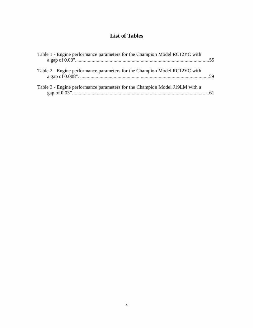
Table 1 - Engine performance parameters for the Champion Model RC12YC witha gap of 0.03". ......................................................................................................55
Table 2 - Engine performance parameters for the Champion Model RC12YC witha gap of 0.008". ....................................................................................................59
Table 3 - Engine performance parameters for the Champion Model J19LM with agap of 0.03”..........................................................................................................61

xi
Nomenclature
Abbreviations and Symbols
AC Alternating Currentb BoreBDC Bottom Dead CenterDC Direct CurrentEa Absolute Errorimep Indicated Mean Effective Pressureisfc Indicated Specific Fuel Consumptionl Connecting Rod LengthLED Light Emitting DiodeMf Fuel Mass Flow RateN Angular Speednf Fuel Conversion EfficiencyNPT National Pipe ThreadnR Crank Revolutions per Power Strokep PowerP PressurePc Cylinder Pressurepsi Pounds Per Square InchP-V Pressure versus VolumeQLHV Lower Heating Valuer Crank LengthRPM Revolutions Per MinuteT TemperatureTDC Top Dead Centerv VoltageV VolumeVcv Clearance VolumeVd Volume DisplacedVI Virtual Instrumentvz Zeroing Voltagew Workx Cylinder Travel

xii
Greek Symbols
∂ Differentialπ Piθ Crank Angle∆ Error
Subscripts
b Brakef Frictioni Indicatedim Intake Manifold
Notation
∫ Integral Absolute Value

1
Chapter 1 - Introduction
Since the development of the first commercially successful steam engine in 1769
by James Watt, engineers and scientists have studied the intra-cylinder phenomena of
reciprocating engines to better understand their principles of operation in order to develop
new methods of optimizing the performance of these versatile power sources [1]. This
research has led to great improvements in the field of internal combustion engines.
For instance, the quality of fuel used to power internal combustion engines has
improved tremendously. Once, it was difficult to predict how a certain batch of fuel
would perform in an engine due to inconsistencies caused by the imprecise production
techniques used to manufacture the fuel. By monitoring the intra-cylinder phenomena
that occurred when different fuels were used, knowledge was gained and discoveries
were made in areas such as the importance of octane rating in fuels. Today, fuels are
produced following strict guidelines so that their performance is predictable and reliable.
Another area that has seen great improvement is the charge induction system.
The most basic system used to mix air and fuel into a combustible mixture and deliver
that mixture to the cylinder is the carburetor. Most carburetors rely on the venturi effect
caused by air being drawn through a restricted passage to draw a measured amount of
fuel into the flow. Analysis of the effects of different carburetor settings and designs on
intra-cylinder phenomena resulted in the carburetor evolving into a complex electronic
device, which is still in use on modern engines. In addition, the development and
perfection of modern electronic fuel injection systems was brought about when the study
of combustion fueled the desire to more precisely control the charge mixture.

2
The charge ignition system ignites the fuel-air mixture in the combustion chamber
of spark ignition engines and is the subject of many ongoing internal combustion engine
research projects. The goal of this system is to ignite the mixture so that it undergoes
complete combustion, which maximizes the energy released by the fuel and minimizes
the production of harmful pollutants. This ignition is normally accomplished by means
of a direct current (DC) system consisting of an ignition coil, which stores a charge that is
then directed to the proper engine cylinder by means of either a rotating distributor or an
electronic ignition system. At the cylinder head, the charge is applied to a spark plug; as
the charge arcs across the gap between the sparkplug electrodes, the mixture is ignited.
This system works well, as long as the mixture surrounding the spark plug gap
contains the proper ratio of air to fuel necessary for successful combustion. One way of
achieving greater efficiency in an engine while decreasing harmful emissions is to burn a
leaner mixture, that is, to use less fuel with the same amount of air for combustion.
However, when this is attempted with a conventional ignition system the result is often
misfires and incomplete combustion. The point where misfires or incomplete combustion
occurs is termed the lean limit, which is approximately equivalent to an air to fuel ratio of
18 for conventional spark ignition engines operating on gasoline [2]. This incomplete
combustion is partially due to the construction of the spark plug. As the flame front
propagates from the point of ignition, the combustible mixture directly behind the arm of
the spark plug electrode is often shielded and therefore may not burn completely.
As a solution to these problems, the Center for Industrial Research Applications at
West Virginia University has proposed a high-energy plasma system to ignite the
mixture. The system consists of a quarter-wave coaxial cavity resonator operating at

3
radio frequencies [3]; an example prototype is shown in Figure 1. This device is capable
of producing a flame volume that is much larger than a conventional DC spark and has
unobstructed contact with the combustible mixture in the cylinder. It is theorized that
this plasma igniter will allow the use of an air-to-fuel mixture that is much leaner than
what is necessary for the use of conventional sparkplugs, therefore allowing the engine to
operate much more efficiently [4].
Figure 1 – The plasma igniter (left) and a conventional spark plug (right).
The plasma ignition system is still in the preliminary design phase, and to
determine if these theories are accurate it is necessary to have a means of quantifying the
performance of an engine into which an ignition system such as the plasma ignition
system can be installed. One method of quantifying the performance of a reciprocating
engine is to calculate the fuel conversion efficiency. This value is a measure of how
effectively an engine converts the chemical energy stored in the supplied fuel to
mechanical energy. To calculate the fuel conversion efficiency, it is necessary to know
the work done by the working fluid in the cylinder. To determine this work value, a plot
of pressure with respect to volume for an individual engine cycle must be produced. This
procedure has been accomplished by using a variety of devices known as indicators. The

4
information provided by these indicators is useful because the engine extracts work from
the working fluid by using the increasing pressure in the cylinder to force the piston
down the bore in an attempt to maintain equilibrium with the crank case pressure.
This relates to the thermodynamic definition of work, which is
∫ ⋅= dVPwi , (1)
where P is the pressure of the working fluid and V is the volume that is occupied by this
fluid. Thus, it can be inferred that the work transferred from the working fluid to the
piston for one engine cycle is equal to the area enclosed by the trace of pressure verses
volume, supplied by the indicator [2]. This value is known as indicated work and can be
used to quantify an engine’s performance.
It should be noted that unless otherwise stated when discussing indicated
quantities in this text, the work is assumed to be the gross work. This definition of work
represents only the work done during the compression and expansion strokes and ignores
any pumping work. This choice was made due to the fact that the research at hand is
primarily concerned with the performance of the engine during the compression and
expansion strokes. In addition, it is possible to perform tests using a dynamometer to
determine values for the brake and frictional work which when summed should
approximate the gross indicated work, thereby allowing the validation of the techniques
used to determine indicated work [2].
Knowing the work, it is possible to determine the indicated power for the given
cylinder. This power is given by

5
R
ii n
Nwp
⋅= , (2)
where N is the angular speed of the engine and nR is the number of crank revolutions for
each power stroke per cylinder [2].
Once the indicated power has been determined, it is possible to calculate the
indicated specific fuel consumption given by
i
f
p
Misfc = , (3)
where Mf is the mass of fuel supplied to the engine per unit time and pi is the indicated
power produced by the engine [2]. The determination of indicated power is discussed
above, and the fuel mass consumed per unit time can be determined by using a scale to
measure the amount of time required to use a given mass of fuel under the current engine
operating conditions.
The fuel conversion efficiency, defined as
)/()/(
3600
kgMJQHkWgisfcn
LHVf ⋅⋅
= , (4)
can now be calculated. The QLHV is the lower heating value of the fuel used in the
engine. For gasoline, the value is approximately 44 MJ/kg [2].
Another value that can be used to quantify the performance of an internal
combustion engine is the indicated mean effective pressure, defined as

6
NV
npimep
d
Ri
⋅⋅= , (5)
where Vd is the volume displaced by the cylinder. The imep is equal to the constant
pressure that, if applied to the cylinder for the entire power stroke, would yield work
equal to the work of the actual cycle [2].
In addition to the many useful calculations that can result from a plot of the
cylinder pressure history with respect to volume, a great deal can be inferred by simple
inspection of these plots. Intra-cylinder phenomena that can be diagnosed in this manner
include knock and poor or nonexistent combustion.
It can be seen that quantifying the performance of an internal combustion engine
relies on the ability to accurately acquire data for the pressure verses volume trace. This
task became increasingly difficult with the development of the first commercially
successful internal combustion engine by Lenoir in 1860 and the modern multi-cylinder
engines into which it evolved [1]. Modern engines typically operate at speeds that are
one hundred times the operating speed of the early internal combustion engines. In
addition, the energy crisis and pollution control laws made necessary the development of
increasingly more efficient engines. Therefore, the technology used to measure and
monitor the engines operating conditions was forced to evolve with the engines.
It is the goal of this work to develop an inexpensive test engine that can be used in
the preliminary testing phases of ignition systems. This system should allow the analysis
of the combustion process, as well as support the determination of values that can be used
to quantify engine performance under the given operating conditions. The work
presented here includes the selection of the engine to be used, the determination and

7
implementation of the instrumentation techniques necessary to meet the goals of this
research, and the analysis of data collected when using different ignition systems in the
test engine.

8
Chapter 2 – Engine Monitoring Techniques
One of the most effective means of quantifying the performance of a given engine
is to develop a plot of cylinder pressure verses volume. By integrating this curve,
indicated power can be determined. Over the years various means have been devised to
produce this plot. A few of the more popular methods are discussed in this chapter.
2.1 Mechanical Indicator
The earliest attempts to monitor the working fluids in the cylinder resulted in the
development of a mechanical indicator in 1796 by John Southern, an assistant to Watt
[1]. The mechanical indicator was attached directly to the head of the engine and could
accurately produce P-V diagrams of the engine cycles for large-displacement, low-speed
engines. Figure 2 depicts the key components of a mechanical indicator [5].
Figure 2 - The key components of a mechanical indicator [5].
The mechanical indicator functioned by measuring the cylinder pressure with an
indicator piston that was loaded by a spring at one end and exposed to the cylinder
pressure at the other via a small passage leading to the combustion chamber. Thus, the
DRUM
WEIGHT
CYLINDER
INDICATORPISTON

9
indicator cylinder displacement was directly proportional to the cylinder pressure. The
cylinder movement was transferred to a pen via a kinematic system. The pen recorded
the pressure data on a drum that rotated at a rate equal to the rate of the volume change in
the cylinder [6]. This task was accomplished by driving the drum with a kinematic
linkage powered by a cyclic engine component, usually the piston or crankshaft [7].
Although the mechanical indicator was considered to be a highly accurate method
of producing pressure verses volume diagrams when properly calibrated for a given low
speed engine, its shortcomings became evident as the operating speeds of internal
combustion engines increased. The increased engine speed inhibited the ability of
mechanical indicators to accurately follow the rapid changes in cylinder pressure and
volume due to inertia and friction of the indicator piston, linkage, and drum. In addition,
the volume of the passage between the clearance volume and the indicator piston was
found to affect the performance of the engine by altering its compression ratio. The same
passage could also be the source of inaccurate data caused by pressure waves resonating
in the passage. Many of the inertia and friction problems were solved by replacing
certain rigid components of the mechanical indicator with an optical system and
recording the data on light sensitive paper, but there was still concern in the engineering
community about the accuracy of mechanical indicators. Therefore, the National Bureau
of Standards developed the balanced pressure indicator [6].
2.2 Balanced Pressure Indicator
The balanced pressure indicator consists of a diaphragm connected to a set of
electrical contacts and a piston-operated recording electrode centered on a rotating drum.
The diaphragm is exposed to engine cylinder pressure on one side and to a set reference

10
pressure on the other. The reference pressure source is normally either a mechanical
pump or some form of compressed gas, usually nitrogen. On the reference pressure side
of the diaphragm, the electrical contacts are mounted in such a way that when the engine
cylinder pressure reaches the reference pressure, the diaphragm moves, and the circuit is
closed. Then when the cylinder pressure drops back below the reference pressure, the
circuit is opened. Closing the electrical circuit results in the generation of a spark that
arcs from the marker point, which is positioned by the action of the reference pressure on
a spring-loaded piston through a piece of paper to a conductive drum. This drum is
driven by the crankshaft so that it is known at exactly what crank angle the pressure
reaches the reference pressure. By slowly varying the reference pressure over the entire
span of engine cylinder pressure, it is possible to produce a complete pressure verses
crank angle diagram [7]. Then if the geometric characteristics of the engine are known,
a pressure verses volume diagram can be produced. The cylinder head unit of a typical
balanced pressure indicator is shown in Figure 3 [7].
Due to the nature of operation of this device, the diagram produced by the
balanced pressure indicator contains an average of data points from many engine cycles.
The cycle-to-cycle variation inherent to spark ignition internal combustion engines
appears as a widening of the pressure data curve produced by a balanced pressure
indicator [7].

11
Figure 3 – The cylinder head pick-up unit of a balanced pressure indicator [7].
This type of indicator is thought to be very accurate and was used to develop
much of the current information concerning intra-cylinder combustion phenomena. A
typical balanced pressure indicator is constructed as depicted in Figure 4 [7].
In addition to its high level of accuracy, the balanced pressure indicator has
several other advantages. It is not susceptible to electrical interference and temperature
effects, and by design it allows the averaging of data from machines with short-term
cycle-to-cycle variations [7].
However, the balanced pressure transducer is not without its disadvantages. It
records pressure with respect to crank angle, therefore necessitating a conversion to
pressure with respect to volume for work calculations. In addition, the amount of time
required to vary the reference pressure across the range of cylinder pressures to obtain a
complete set of data and then compile it is many times greater than the time required to
obtain similar results with other available methods. Probably the greatest single
BALANCEPRESSURE
CONNECTION
ELECTRICALCONNECTION
DIAPHRAMCONTACT

12
drawback of the balanced pressure transducer is its inability to measure and record the
intra-cylinder data for a single engine cycle [7]. This data is very important to the study
of phenomena such as engine knock. Therefore, many researchers began experimenting
with new technology brought about by the availability of economical microprocessors,
and the result was the development of high-speed electronic indicating systems.
Figure 4 – Layout of a balanced pressure indicator system [7].
2.3 Electronic Indicating Systems
Electronic indicating systems have been developed to instantaneously acquire and
record cylinder pressure data at multiple points during a single engine cycle, thus
allowing researchers the ability to accurately map the cycle and study the combustion
phenomena based on this single cycle. Electronic indicators have been designed using a
wide variety of hardware, but they all share the same general components, namely a
PRESSUREPUMP
CYLINDER HEADPICK-UP UNIT
(SEE FIGURE 2)
COUPLED TOCRANKSHAFT
DRUM
MARKINGPOINT
POWERSUPPLY
SPRINGPISTON

13
power supply, a motion transducer, a pressure transducer, and a readout or recording
device.
2.3.1 Motion Transducers
One of the greatest obstacles that had to be overcome during the development of
electronic indicator systems was the problem of acquiring accurate data concerning the
piston position and synchronizing that data with the cylinder pressure data. Several
schemes for accomplishing this task have been devised. One early method involved the
mounting of a number of AC generators to the crankshaft and using their output to
generate engine position data [8]. Another technique, which was employed by Caterpillar
Tractor Company researchers, involved using a photocell to measure the intensity of light
shining through a slot that was partially blocked by a cam driven by the crankshaft [9].
These methods were functional but lacked the precision necessary for accurate
combustion analysis. The development of the optical shaft encoder provided researchers
the required accuracy.
Optical shaft encoders consist of an LED source, a photocell, and a slotted disk.
The disk separates the light source from the photocell and is driven by the crankshaft.
The unit produces a square wave every time a slot passes by the photocell. Therefore, the
number of slots in the disk determines the resolution of the encoder. Encoders are
currently commercially available in resolutions up to 60,000 counts per revolution. In
addition, most commercial optical encoders are available with a reference signal that
occurs once per revolution. The system can be set up so that the reference signal occurs
precisely when the engine is at top dead center (TDC). By monitoring the number of

14
counts occurring since TDC, the crank angle and corresponding piston position can be
determined.
2.3.2 Pressure Transducers
An electronic pressure transducer produces an electrical signal proportional to the
pressure the sensor is exposed to. Many different types of electronic pressure transducers
have been developed, each operating on a different scientific principle. The most popular
of these designs have been the strain gage type and the piezoelectric type.
The strain gage type is constructed by mounting a thin metal diaphragm across a
hollow tube. Strain gages are then mounted to measure the deformation as the pressure
differential across the diaphragm changes. These transducers can be very accurate;
however, the frequency response of this type of transducer is generally too slow for many
internal combustion engine applications.
Since it is small, lightweight, and has a high frequency response, the piezoelectric
charge mode pressure transducer, as shown in Figure 5 [10], is the sensor of choice for
most researchers. It is made up of a housing containing a quartz element surrounding an
electrode. As the pressure applied to the unit changes, the piezoelectric properties of the
quartz produce a static charge that is linearly proportional to the change in pressure. This
charge can then be amplified and recorded to obtain an accurate record of the changes in
the pressure applied to the unit.
The main shortcoming of the piezoelectric charge mode pressure transducer is
that it measures the changes in pressure rather than measuring the absolute pressure.
Consequently, an accurate baseline for the pressure data must be determined. The
simplest method to accomplish this is to assume that the pressure at the completion of the

15
intake stroke is equal to the average intake manifold pressure, which can be measured
with a transducer or manometer [11]. Care must also be taken when mounting this type
of transducer since it can be adversely affected by rapid changes in temperature, which
could be caused by hot combustion gasses coming into contact with the sensor. In
addition, these transducers are susceptible to temperature response errors caused by small
changes in the transducer temperature. Care must be taken to minimize these errors in
experimental work.
Figure 5 – Cross-section of a piezoelectric pressure transducer [10].
2.3.3 Readout and Recording Devices
Early researchers utilized oscilloscopes and oscillographs as readout and
recording devices. However, due to the availability of economical high-speed
microcomputers these methods are virtually obsolete. A variety of manufacturers
produce data acquisition boards that interface with personal computers, allowing the
researcher to monitor a number of analog signals at millions of samples per second.
ELECTRICALCONNECTION
QUARTZELEMENT
ELECTRODE
HOUSING

16
Various computer software packages can then be used to compile and analyze the stored
experimental data.
2.4 Temperature Measurement
Often, it is necessary to monitor certain operating temperatures of an engine. The
most important of these are the intake air and the exhaust gas temperatures. The
measurement of the intake air temperature is important because it allows any
performance quantifying values that are determined for the engine to be corrected for
standard ambient conditions. The temperature of the exhaust gas can be used as a tool to
determine engine combustion efficiency. For instance, if engine combustion efficiency
increases, then there should be more energy released in the cylinder, which will cause the
exhaust temperature to rise due to more energy being lost in the form of heat. There are a
number of devices available that can accurately measure such temperatures, the most
common of which are the resistance temperature detector, thermistor, and thermocouple.
2.4.1 RTDs
Resistance temperature detectors, or RTDs, were first developed in 1821 by
Humphrey Davy [12]. They operate on the principle that certain metals display a highly
predictable change in resistivity as their temperature changes. Therefore, by properly
monitoring the resistance of a thin wire, it is possible to determine accurately the
temperature of that wire. The most common materials for this application are platinum
and nickel, with platinum being the more accurate as well as the more expensive.
While RTDs are capable of measuring temperatures with a great deal of precision,
and have response times of less than one tenth of a second, they are limited to maximum

17
temperatures of around 593 °C. For this reason, they are not the devices of choice for
many internal combustion engine applications [12].
2.4.2 Thermistors
A thermistor is another temperature measuring device that operates on the
principle of temperature dependant resistance. However, unlike the wire elements used
in RTDs, the element used in a thermistor is made of a semi-conductor material. They
are by far the most accurate of the temperature measuring devices; however, they are
extremely fragile and are limited by response times of several seconds and maximum
temperatures of around 100 °C. It is for these reasons that thermistors have limited
usefulness in the field of internal combustion engine monitoring [12].
2.4.3 Thermocouples
The thermocouple is by far the most versatile of the temperature measuring
devices. It operates on the thermoelectric principle discovered by Thomas Seebeck in
1821 [12]. Seebeck observed that when two wires made of dissimilar metals are joined at
both ends and one end is heated, there is a continuous current that flows in the
thermoelectric circuit. If the circuit is broken at the center, the voltage difference
between the wires is a function of the junction temperature and the composition of the
two metals. Therefore, by measuring this voltage the temperature at the junction can be
determined.
However, this voltage cannot simply be measured with a voltmeter because doing
so creates a second thermoelectric circuit, thus corrupting the data. To correct for this
phenomenon, is necessary to control the temperature of the junction between the
voltmeter and the thermocouple. This can be done by placing the junction in an ice bath,

18
thereby holding its temperature at 0 °C, or more practically by utilizing an electronic ice
point compensator. This device uses a battery to create a voltage that mimics placing the
reference junction in an ice bath, and therefore greatly simplifies the use of
thermocouples.
The relationship between thermocouple voltage output and junction temperature
is nonlinear, but it can be accurately modeled by a higher order polynomial function.
This somewhat complicates the use of thermocouples as temperature monitoring devices,
but these polynomial equations are readily available for the thermocouples and are easily
programmed into personal computers for data acquisition applications. Depending on the
type of metals used, thermocouples are available that can measure temperatures up to
1815 °C with an error of less than 2 °C. This, along with the fact that they are extremely
rugged and inexpensive, makes thermocouples the logical choice for most internal
combustion engine temperature measurement applications [12].
19
Chapter 3 – Hardware
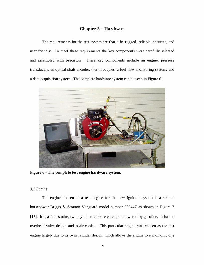
The requirements for the test system are that it be rugged, reliable, accurate, and
user friendly. To meet these requirements the key components were carefully selected
and assembled with precision. These key components include an engine, pressure
transducers, an optical shaft encoder, thermocouples, a fuel flow monitoring system, and
a data acquisition system. The complete hardware system can be seen in Figure 6.
Figure 6 - The complete test engine hardware system.
3.1 Engine
The engine chosen as a test engine for the new ignition system is a sixteen
horsepower Briggs & Stratton Vanguard model number 303447 as shown in Figure 7
[15]. It is a four-stroke, twin cylinder, carbureted engine powered by gasoline. It has an
overhead valve design and is air-cooled. This particular engine was chosen as the test
engine largely due to its twin cylinder design, which allows the engine to run on only one

20
cylinder. This feature is useful for the initial testing phases of ignition system. The
engine was donated to the Center for Industrial Research Applications by Briggs &
Stratton Corporation.
Figure 7 - The Briggs & Stratton Vanguard Engine [15].
The engine specifications state that it has a total displacement of 29.3 in3 and is
capable of producing a maximum torque of 24.3 ft-lbs at an engine speed of 2400-RPM
[16]. The major modifications to the engine include the removal of the manual start
mechanism to facilitate the mounting an optical encoder to the crankshaft and the tapping
of the cylinder head to accept a pressure transducer. In addition, the exhaust manifold is
tapped to mount a thermocouple and both a thermocouple and pressure transducer are
mounted in the intake manifold.
3.2 Pressure Transducers
Two pressure transducers are utilized in the completed test engine. The first
transducer is a PCB model 112B11. It is mounted directly into the cylinder head and is
used to monitor the cylinder pressure throughout the engine cycle. The second is an
Omega model PX 126-015-V. It is mounted in the intake manifold and is used to acquire

21
the baseline necessary to establish the absolute values for the pressure curve produced by
the cylinder head transducer.
3.2.1 PCB Model 112B11
The Model 112B11 pressure transducer is manufactured by PCB Piezotronics. It
is a piezoelectric charge mode transducer; it contains a quartz crystal that produces a
static charge when the pressure applied to its surface changes. This particular transducer
was chosen for its small size, as can be seen in Figure 8, as well as for its accuracy and
quick response time [17].
Figure 8 - Housing Design of a PCB Model 112B11 Pressure Transducer [17].
The manufacturer’s specifications state that this transducer weighs only .2 ounces,
has a resolution of .01 psi, and has a rise time of 3 microseconds [18]. These accuracy
and response time values are more than adequate for monitoring the high cylinder
pressures in this relatively low speed engine.
To mount the transducer in the test engine, a mounting hole and orifice were
drilled and tapped in accordance with the suggested mounting procedure as described in
the Operator’s Manual supplied by the manufacturer [18]. The orifice enters the
combustion chamber through the outboard surface of the cylinder head in the position
indicated in Figure 9. This position was chosen because it allowed easy access for

22
transducer maintenance and allowed for the modifications to be made in the area of the
head with the most material, thus preserving the structural integrity of the cylinder head.
⊕
Figure 9 - Cylinder head transducer placement.
For the initial development of the test engine, only one cylinder was instrumented.
However, the instrumentation of the other cylinder could easily be accomplished using
the same techniques discussed in this work.
Since this type of transducer produces a high impedance charge, several
additional pieces of equipment are necessary to transform the signal into a low
impedance voltage that can be monitored by a data acquisition system. Those pieces of
equipment are an in-line charge amplifier and a line power supply/signal conditioner.
The complete PCB system is shown in Figure 10.
⊕ = Transducer Position

23
Figure 10 - The complete PCB pressure transducer system.
3.2.2 Omega Model PX 126-015D-V
As stated previously, when using a piezoelectric charge mode transducer it is
necessary to determine an accurate baseline to establish the absolute values for the points
on the pressure trace. It has been suggested that one accurate method of doing this is to
set the pressure at BDC on the intake stroke equal to the average intake manifold pressure
[11]. Therefore, in order to determine the average manifold pressure in the test engine,
an Omega model PX 126-015-V pressure transducer, such as the one shown in Figure 11,
is connected to the intake manifold by means of a length of PVC tubing and a 1/4 inch
NPT barbed tubing fitting.
This transducer operates on the principle of piezoresistivity, which means that the
resistivity of the sensing element changes proportionally with the changes in the pressure
that is applied to it. The heart of the transducer is a 0.1 inch square silicon chip.
Embedded in this chip is a sensing diaphragm and piezoresistors. As the pressure
changes, the diaphragm flexes causing the resistance values to change. The
piezoresistors are connected to a four-active-member Wheatstone bridge allowing the
In-Line Charge Amplifier
Low Noise CablePower Supply/Signal Conditioner
Pressure Transducer

24
transducer to measure differential pressures between 0 and 15 psi with a maximum error
of 0.5 psi and a response time of one millisecond [19].
Figure 11 - The Omega model PX 126-015-V pressure transducer.
3.3 Optical Shaft Encoder
As mentioned previously, one of the major problems in the development of an
electrical indicator system is developing a method of acquiring accurate data concerning
the piston position and synchronizing that data with the cylinder pressure data. To
accomplish this, the manual start mechanism was removed from the engine, and a custom
flywheel retainer bolt was used to replace the original factory bolt. This custom bolt
incorporated a 1/2” extension shaft, which allowed an Accu-Coder size 15 model 755A
hollow shaft flexible mount incremental encoder, such as the one shown in Figure 12, to
be directly coupled to the crankshaft [20].

25
Figure 12 - The Accu-Coder model 755A incremental shaft encoder [20].
The Accu-Coder model 755A operates by means of a slotted disk that rotates
between a photocell and an LED. This particular encoder has 1000 slots in the disk.
When one of these slots passes in front of the photocell, light from the LED is allowed to
pass through to the photocell, thus triggering a pulse output. The pulse activates an NPN
pull up resistor circuit that is connected to an external 5-volt source. The result is a
square wave that displays 1000 pulses per revolution, allowing the shaft angle to be
determined to within 0.36 degrees. In addition, there is a second channel and a reference
channel that operate on the same principle as the first. The output of the second channel
lags the output of the first signal by a phase difference of ninety degrees and can be used
to determine the direction of rotation for certain applications; it was not used for this
work. The reference channel displays only one pulse per revolution [20].
The encoder was installed so that the occurrence of the reference signal
corresponds to the piston being at top dead center in the cylinder. This was accomplished
by first positioning the engine crank so that the piston was at exactly top dead center.
This position was determined by mounting a dial indicator in such a way that its shaft
went through the spark plug mounting hole and made contact with the piston. The engine
was then turned until it was roughly estimated to be at top dead center; this position is

26
approximate due to the small amount of piston travel that corresponds to considerable
crank shaft rotation when the piston nears top dead center. The position was marked on
the flywheel using a custom built rigid pointer that was installed on the engine as shown
in Figure 13.
Figure 13 - The rigid pointer used to determine top dead center of the engine.
The exact top dead center of the engine was then determined using the procedure
described in the ASME test codes for the measurement of indicated power [7]. First, the
engine was turned clockwise to a position that was approximately twenty degrees before
top dead center. Using the pointer, this position was marked on the flywheel and the dial
indicator was zeroed. Next, the engine was turned clockwise until the dial indicator
passed top dead center and passed the zero reading. The engine was then turned counter
clockwise until the dial indicator returned to the zero reading. This position was also
marked using the pointer. Bisecting the angle between these two marks allowed an
accurate mark indicating top dead center to be produced. This mark was lined up with
the pointer, and the encoder was rotated until the reference signal point was reached. The

27
encoder was then firmly coupled to the crankshaft by tightening the two set-screws on the
encoder collar.
With the encoder synchronized with top dead center, it is possible to use the
reference pulse to trigger the data acquisition system to begin taking data at top dead
center. In addition, the 1000 counts per revolution square wave produced by the encoder
can be used as an external clock to time the data acquisition, which allows the engine
pressure data to be precisely synchronized with the cylinder volume data.
3.4 Thermocouples
Two thermocouples are utilized in the instrumentation of the test engine. They
are both Omega model KQSS-18E-12 quick disconnect thermocouples. These
thermocouples are type K, which means that they are capable of measuring temperatures
from –200 °C to 1250 °C with a maximum error of 0.75% of the measured temperature
value [12]. This type of thermocouple was chosen because the temperatures to be
measured were predicted to fall into this range. Coupled to each thermocouple is an
Omega model MCJ-K miniature electronic ice point device. As discussed earlier, this
device provides a voltage that is equivalent to placing the reference junction of the
thermocouple into an ice bath. The entire temperature measurement system can be seen
in Figure 14.
Figure 14 - The Omega model KQSS-18E-12 thermocouple and Omega model MCJ-K ice point device.

28
The first thermocouple is mounted in the intake manifold, thereby allowing it to
monitor the intake air temperature. It was mounted by drilling and tapping the manifold
to accept a 1/4” NPT x 1/8” compression fitting. In order to allow the thermocouple to
pass completely through the fitting to reach the center of the manifold, it was necessary to
enlarge the center of the fitting using a 1/8” drill bit. The second thermocouple is
mounted in the exhaust manifold, allowing it to monitor the exhaust gas temperature. It
was mounted by welding a similar 1/4” NPT x 1/8” compression fitting to the exhaust
manifold. Once again, it was necessary to enlarge the center of the fitting to accept the
1/8” thermocouple.
3.5 Fuel Flow Monitoring System
In order to calculate the indicated specific fuel consumption, it is necessary to
determine accurately the mass of fuel that is consumed by the engine per unit time under
the given operating conditions. To accomplish this, the engine is supplied with fuel from
a 1000-ml beaker. The beaker rests on an Ainsworth model 400 digital scale that is
calibrated in grams. This allows the mass of fuel used by the engine over a given length
of time to be measured, so the mass fuel consumption per unit time can be calculated.
One of the most important features of the fuel monitoring system is the fuel line support
stand. This stand is a tripod structure that straddles the scale supporting the fuel line so
that it does not rest on the beaker, which would cause an error in the fuel mass
measurements. The entire fuel flow monitoring system can be seen in Figure 15.

29
Figure 15 - The fuel flow measuring system.
3.6 Data Acquisition System
In order to collect data from the array of transducers used to monitor the operation
of the test engine, it was necessary to utilize an electronic data acquisition system. This
system is capable of monitoring the output of every transducer simultaneously at an
acquisition rate that is great enough to allow the collection of data at maximum engine
speed. The heart of this system is a National Instruments model DAQCard-A1-16E data
acquisition card such as the one shown in Figure 16.

30
Figure 16 - The National Instruments model DAQcard-A1-16E-4 data acquisitioncard.
This card is placed into the PCMCIA drive of the 200 MHz Kapok Computer
Company model 7200 notebook computer that is used to acquire and compile the engine
data. It is then connected by a shielded cable to a terminal block. The various
transducers are then connected to this terminal block, allowing the transducers to
interface and communicate with the computer. A wiring diagram that displays the
necessary terminal block connections is shown in Figure 17. The DAQcard-A1-16E-4 is
capable of monitoring 16 single ended or 8 differential analog input channels with 12-bit
resolution. Gains are available from .5 to 100 and are channel independent. It is capable
of sampling at rates up to 500,000 samples per second for single channel sampling and
250,000 samples per second for multi-channel scanning. It also allows both analog and
digital triggering of the data acquisition, which is necessary for the test engine application
[21].

31
Figure 17 - Wiring diagram for the data acquisition system.
Reference
Channel A
Common Ground
+
_
+
+
+
_
_
_

32
Chapter 4 – Software
The numerous transducers and engine monitoring systems that are used to
quantify the engine’s performance supply a tremendous amount of information to the
DAQ-A1-16E-4 card in the form of analog signals. In order to collect and compile this
information, a number of software packages are utilized. The collection and storage of
raw data is controlled by Labview [22] while the data is compiled into a more user
friendly format and analyzed using Microsoft Excel [23] and Matlab [24].
4.1 Data Collection Software
Labview, the program that controls the data acquisition card, is a software
package that automates laboratory instrumentation and data acquisition. With Labview
and the proper data acquisition card, a researcher controls on the PC what was once a
laboratory full of electronic equipment. With Labview, it is possible to create customized
virtual instruments or VIs. For the test engine development it was necessary to develop
two separate virtual instruments. The first virtual instrument is used for acquiring and
storing the intra-cylinder data such as the cylinder pressure and shaft position (volume),
while the second monitors the parameters external to the cylinder, those being intake
temperature, intake pressure, and exhaust temperature.
Labview virtual instruments consist of two windows. The first is the instrument
diagram, which is a schematic representation of the instrument showing the individual
components, how they are virtually connected, and how they interact with one another.
The second screen is the instrument control panel. Through this screen, variables are
input to the instrument, the instrument is operated, and the resulting output is displayed.

33
4.1.1 The Intra-cylinder Data VI
The intra-cylinder data virtual instrument for this test engine application was
created to allow digital triggering of the data acquisition. Digital triggering was
necessary to allow the optical shaft encoder reference signal to trigger the start of data
acquisition, thus beginning data acquisition at top dead center. In addition, the VI
employs an external counter clock. This feature allows the signal from the optical
encoder to be used to trigger the acquisition of each data point. Therefore, the exact
piston position at the time of data acquisition is known.
This virtual instrument also allows the acquired data to be saved to a user
specified file in a comma delimited format, allowing the data to be transferred to a
spreadsheet program for analysis. The instrument diagram for this VI can be seen in
Figure 18.
Figure 18 - The instrument diagram for the intra-cylinder data VI.

34
The control panel for the VI is shown in Figure 19. It displays windows for
entering the trigger type, device number, channels, number of scans to acquire, pretrigger
scans, input limits, trigger edge, and time limit.
Figure 19 - The control panel for the intra-cylinder data VI.
The trigger type window allows two choices, the first is Start or Stop Trigger and
the second is Start and Stop Trigger. The Start or Stop Trigger choice allows the digital
trigger signal to either stop or start the data acquisition depending on the value entered
into the pretrigger scans window. If the pretrigger scans value is zero, then the external
signal will trigger the start of data acquisition, and acquisition will terminate when the
desired amount of data is collected. If the pretrigger scans value is greater than zero, then
the software starts the data acquisition and waits for the stop trigger. The program then
stores the amount of data that corresponds to the pretrigger scans value and records the

35
remainder of the data after the trigger. This setting is useful if the researcher is interested
in acquiring data both before and after the trigger signal. If the trigger type window is set
to Start and Stop Trigger, then the pretrigger scans value must be greater than zero. The
data acquisition is started by the first trigger signal, and then when the second trigger
signal occurs, the program stores the amount of data that corresponds to the pretrigger
scans value and records the remainder of the data after the trigger.
The device number determines which data acquisition card is to be activated by
the instrument to take the data, while the channels window informs the instrument of
which channels on that card are to be monitored. The number of scans to acquire
determines the amount of data to be collected before data acquisition is terminated. The
input limits window allows the user to set values for the extreme limits of the input
signals for each channel. These values are then used by the software to automatically set
gain values for maximum accuracy. The trigger edge window can be set to trigger on
either the rising edge of the input signal, the falling edge of the input signal, or when
there is no change in the input signal. The time limit window allows the user to set a
limit as to how long the instrument will wait for a trigger signal. This feature provides a
means to terminate the instrument run if a hardware problem should occur. In addition to
these input windows, a graphical display is provided to exhibit the acquired data traces.
4.1.2 The Extra-cylinder Data VI
The extra-cylinder data virtual instrument for the test engine was created to allow
a number of input signals to be monitored using the PC clock as a timing signal. This
gives the user a real-time reference with which to determine engine speed. In addition,
signals that do not need to be synchronized with piston position, such as intake and

36
exhaust parameters, are monitored using this VI to allow for maximum acquisition speed
when monitoring the engine with the intra-cylinder data VI. The instrument diagram for
this VI can be seen in Figure 20.
Figure 20 - The instrument diagram for the extra-cylinder data VI.
The control panel for the extra-cylinder data VI is shown in Figure 21. It displays
windows for entering device number, channels, number of scans to acquire, scan rate, and
input limits. Just as with the intra-cylinder VI, the device number determines which data
acquisition card is to be activated by the instrument to take the data, while the channels
window informs the instrument of which channels on that card are to be monitored. The
number of scans to acquire determines the amount of data to be collected before data
acquisition is terminated. The scan rate window allows the user to set the speed at which
data will be acquired in scans per second. This value is restricted by the capability of the

37
card. Its value cannot be greater than the maximum speed of the card divided by the
number of channels to be monitored. In the case of this system, the maximum value is
62,500 scans per second. The input limits window allows the user to set values for the
extreme limits of the input signals for each channel. These values are then used by the
software to set gain values for maximum accuracy. Again, in addition to these input
windows, a graphical display is provided to exhibit the acquired data traces.
Figure 21 - The control panel for the extra-cylinder data VI.
4.2 Data Analysis Software
After data has been secured from the engine transducers by Labview, it is
transferred to an Excel spreadsheet. While Labview does have the capability of
performing the data analysis, the decision was made to perform these tasks in Excel and

38
Matlab for the ease of data manipulation that they provide. Once the data is transferred, a
set of custom macros that were created using Excel’s macro recording feature are applied
to the data files.
The first macro can be found in Appendix A and is used to compile the engine
pressure and position data. It first applies a five point moving average to the data set.
This reduces the amount of noise that is found in the data signal. Next, the macro
repositions the information into the first 8000 rows of the spreadsheet. This is necessary
to allow the next step of the macro, which is saving the file to the Matlab directory in a
“filename.wk1” format. This format allows the file to be opened by Matlab.
The second macro can be found in Appendix B and is used to compile the engine
speed, exhaust, and intake data. It first determines average values for the intake
temperature, intake pressure, and exhaust temperature. Next, it places this data along
with the engine speed data into the first 8000 rows of the spreadsheet and saves the file in
“filename.wk1” format in the Matlab directory so that it can be opened by Matlab.
Once the engine data has been processed through the spreadsheet macros, the
Matlab program Engine.m as shown in Appendix C is executed. This program first asks
the user to input the fuel consumption of the engine in grams per minute under the current
operating conditions. This information is obtained by using the digital scale to monitor
fuel flow during testing. Next, the program opens both of the data files and arranges the
data points into the proper arrays. The speed of the engine is then calculated using the
reference signal from the Accu-Coder model 755A optical encoder that is recorded by the
extra-cylinder data VI. This calculation is carried out by first using a counter routine to
step through the data file and mark the sample numbers where the reference signal

39
occurs. These values should correspond to top dead center of the engine. Then, since it
is known that the data was recorded at 62,500 samples per second, the revolutions per
minute can be calculated by using:
12
6062500
TDCTDCRPM
−⋅= , (6)
where TDC1 is the data point number where the first reference signal occurred, and
TDC2 is the data point number where the second reference number occurred. This
procedure is carried out for the entire data set, and an average value for the speed of the
engine is calculated.
Next, the program uses the other data recorded by the extra-cylinder data VI to
determine the intake manifold air pressure, the intake manifold air temperature, and the
exhaust manifold air temperature.
To calculate intake manifold air pressure, the absolute value of the signal from the
Omega model PX 126-015-V pressure transducer is determined. This is necessary
because the transducer is measuring vacuum pressure; therefore, its output signal is
negative. The Omega model PX 126-015-V is designed to have linear output over a
range of 0 to 15 psi differential pressure, and it is designed to have a full scale output that
is equal to 10 milli-volts for every volt of supply power [19]. Since the transducer is
powered by an automotive battery measuring 12.3 VDC, the intake manifold pressure in
pounds per square inch can be calculated by substituting the value of the transducer
output into the equation:
123.
157.14 1⋅−= v
pim , (7)

40
where v1 is the absolute value of the signal from the transducer in volts.
To determine the intake and exhaust manifold temperatures, the program first
retrieves the output of the respective Omega model KQSS-18E-12 thermocouple and
Omega model MCJ-K ice point device systems. Then, since the output of the
thermocouple system does not vary linearly with temperature, the polynomial equation:
,)1333708.6()133869.1(
)1218452.1()1083506.4(9.860963914
682.22103404248.67233109.24152226584602.0
82
72
62
52
42
32
222
vEvE
vEvEv
vvvT
⋅+−⋅++
⋅+−⋅++⋅−
⋅+⋅+⋅+=
(8)
where T is the temperature in degrees Celsius and v2 is the output of the thermocouple
system in volts, must be used to calculate the temperatures [12].
The next stage of the program is concerned with beginning the analysis at top
dead center (TDC) on the intake stroke. To determine this point, the program looks at the
pressure data for the first two TDC points. It then picks the one with the lowest pressure
and marks it as TDC1. The remaining TDC points are then located and labeled by adding
1000 to the previous TDC value. This technique works because the encoder pulses that
trigger the acquisition of each data point have a resolution of 1000 pulses per revolution.
Once the TDC values have been labeled, the program proceeds to convert the
pressure data into units of pressure and shift these pressure curves so that the pressure at
the completion of the intake stroke is equal to the average manifold air pressure [11]. To
accomplish this, first five data points are at the end of the intake stroke by adding
496…500 to the respective intake TDC values. The output of the PCB Model 112B11
pressure transducer for these data points is then averaged to obtain a “zeroing” value.
That is a value that when subtracted from the entire pressure curve will shift that curve so

41
that the end of the intake stroke lies on the x-axis. Using the average of five data points
for this “zeroing” value protects the true pressure trace from being corrupted by noise in
the signal. Once the pressure trace is “zeroed,” then the intake manifold air pressure can
be added to the curve, causing it to shift an amount that creates an accurate trace of
absolute cylinder pressure when the appropriate conversion factors are applied to the
data. These conversion factors are specific to the individual transducer calibration. The
final equation for cylinder pressure in pounds per square inch that is applied to the entire
pressure data array for the individual engine cycles appears as:
imz
c Pvv
P +⋅−=08216.1
1000)( 3, (9)
where v3 is the output of the pressure transducer in volts, vz is the zeroing value in volts,
and Pim is the intake manifold pressure in pounds per square inch [18].
The next stage of the program creates an array of crank angles from 0 to 4π
radians in increments of 2π/1000 for each engine cycle. Each crank angle value then
corresponds to a pressure data point since the pressure data acquisition was triggered by
the optical encoder every 2π/1000 radians. Once the crank angle arrays have been
created, then if the physical parameters of the engine are known they can be transformed
into cylinder volume arrays. This is done by applying the equations:
)sin(cos 222 θθ ⋅−+⋅= rlrx (10)
and

42
)(4
2
xrlb
VV cv −+⋅⋅+= π , (11)
where x is the distance of the piston from TDC in inches, r is the distance from the center
of the crank pin to the center of the main pin in inches, θ is the crank angle in radians, l is
the length of the connecting rod in inches, V is the cylinder volume in cubic inches, Vcv is
the clearance volume in cubic inches, and b is the bore of the cylinder in inches [2]. The
physical dimensions of the engine components, with the exception of clearance volume,
were obtained by contacting Briggs & Stratton Corporation customer service. From
Heywood [2] it was determined that a typical compression ratio for an engine of this type
and size is 7, so the clearance volume was assumed to be 2.45 cubic inches, which
provides this compression ratio. This assumption will be proved valid later in this work.
The pressure and volume arrays for each cycle are then divided into separate
arrays for the intake, compression, expansion, and exhaust strokes. From Equation 1, it is
known that the integral, or area under the plot of pressure versus volume, can be used to
determine indicated horsepower. This area is calculated by using the TRAPZ function in
Matlab. This function utilizes trapezoidal numerical integration to determine the area
under each curve. The program then calculates the gross indicated work for the cylinder
by subtracting the area under the compression stroke from the area under the expansion
stroke. This results in the total area enclosed by the power loop, which is equal to the
gross indicated power. The program also calculates the net indicated power, which is the
area enclosed by the pumping loop subtracted from the gross indicated power. Since this
work is primarily concerned with gross engine parameters, this quantity is not currently

43
utilized by the program; however, its availability allows the program to be easily
modified to analyze net engine parameters.
With the gross indicated work for each cycle calculated, the program then
calculates the gross indicated power for each cycle using Equation 2. This allows the
program to apply Equations 3, 4, and 5 to calculate the indicated specific fuel
consumption, fuel conversion efficiency, and indicated mean effective pressure for each
cycle. The program then displays the calculated values to the user, and through a
graphical user interface, allows the user to request a pressure verses volume plot, such as
the one shown in Figure 22, for any of the cycles.
Figure 22 - A pressure versus volume plot produced by Engine.m.

44
Chapter 5 – System Accuracy Verification
To provide a degree of confidence in the results obtained from this research, it is
necessary to determine and quantify possible sources of inaccuracy in the acquired data.
Two such sources of inaccuracy are the phasing of volume data with the pressure data
and the assumed value for the clearance volume. A test to determine the accuracy of
these parameters has been defined by Randolph [11]. It involves plotting the pressure
versus volume history that is created as the engine is motored on a log-log scale. If the
resulting graph shows the lines corresponding to the compression and expansion stroke
crossing, then the pressure and volume data is not phased properly. If this graph shows
curvature of the compression and expansion lines, it can be concluded that the value for
the clearance volume of the cylinder is incorrect. A plot with a correct value for the
clearance volume displays linear compression and expansion curves.
To acquire the necessary data, the engine was coupled to a General Electric model
5T20GA5 DC cradled dynamometer as seen in Figure 23. This dynamometer allowed
the engine to be motored at its normal operating speed.
Unfortunately, due to the condition of the available dynamometer, it was only
possible to motor the engine, and little else. Had it been possible to load the engine and
measure the corresponding torque, an additional test for accuracy would be to first arrive
at an estimate for the power necessary to perform the pumping work as well as overcome
the internal friction of the engine. This value is called the friction power, which could be
determined by measuring the power input from the dynamometer to the engine during
motoring. Next, the engine could be loaded, data taken, and the corresponding brake

45
power measured by the dynamometer. The resulting values should correspond with the
equation:
fbi ppp += , 12
where pi is the indicated power given by running Engine.m, pb is the brake power
measured by the dynamometer, and pf is the friction power measured while motoring the
engine, which will include the power necessary to overcome mechanical friction as well
as the pumping power [2]. The fact that the test engine was designed to be completely
mobile will allow this test to be performed should a suitable dynamometer become
available.
Figure 23 - The test engine coupled to the General Electric DC CradledDynamometer.

46
The pressure and volume data sets resulting from the motoring test were plotted,
and it was noticed that the compression and expansion curves did indeed cross near the
center of the strokes. An attempt was made to correct this error by shifting the volume
data one point. This improved the situation but did not alleviate it. When the volume
data was shifted one additional point, the curves no longer crossed as can be seen in
Figure 24. The data analysis program was then modified to perform the shift to correct
for this error. Thus it can be concluded that the phasing of the pressure and volume data
is accurate to within one volume unit. Since a sample is triggered 1000 time per
revolution, the resulting phase shift is equal to 360/1000 degrees. This error is of great
concern when computing mean effective pressures. However, previous research has
shown that this is accurate enough for this type of research [25]. In addition, it can be
seen that the curves corresponding to compression and expansion in Figure 24 are indeed
linear, which validates the assumption of a 2.45 cubic inch clearance volume.

47
Figure 24 - A log-log plot of pressure versus volume for the motored engine cycle.
Another possible source of inaccuracy is the five point moving average that is
applied by the intra-cylinder data macro to the output data from the piezoelectric pressure
transducer. This routine is meant to smooth the noise in the data. This noise in inherent
to piezoelectric pressure transducers, especially at low cylinder pressures. It is believed
that this phenomenon may be due to the turbulent flow of working fluid near the sensor
[25]. Figure 25 shows a small section of the piezoelectric pressure transducer output
signal along with the results of the five point moving average. From this plot, it is clear
that the moving average curve shows a significant improvement over the original curve.
It was found that the maximum difference between the actual output and the moving
average at peak pressure was on the order of 1%. This possible error was found to be
Compression
Expansion
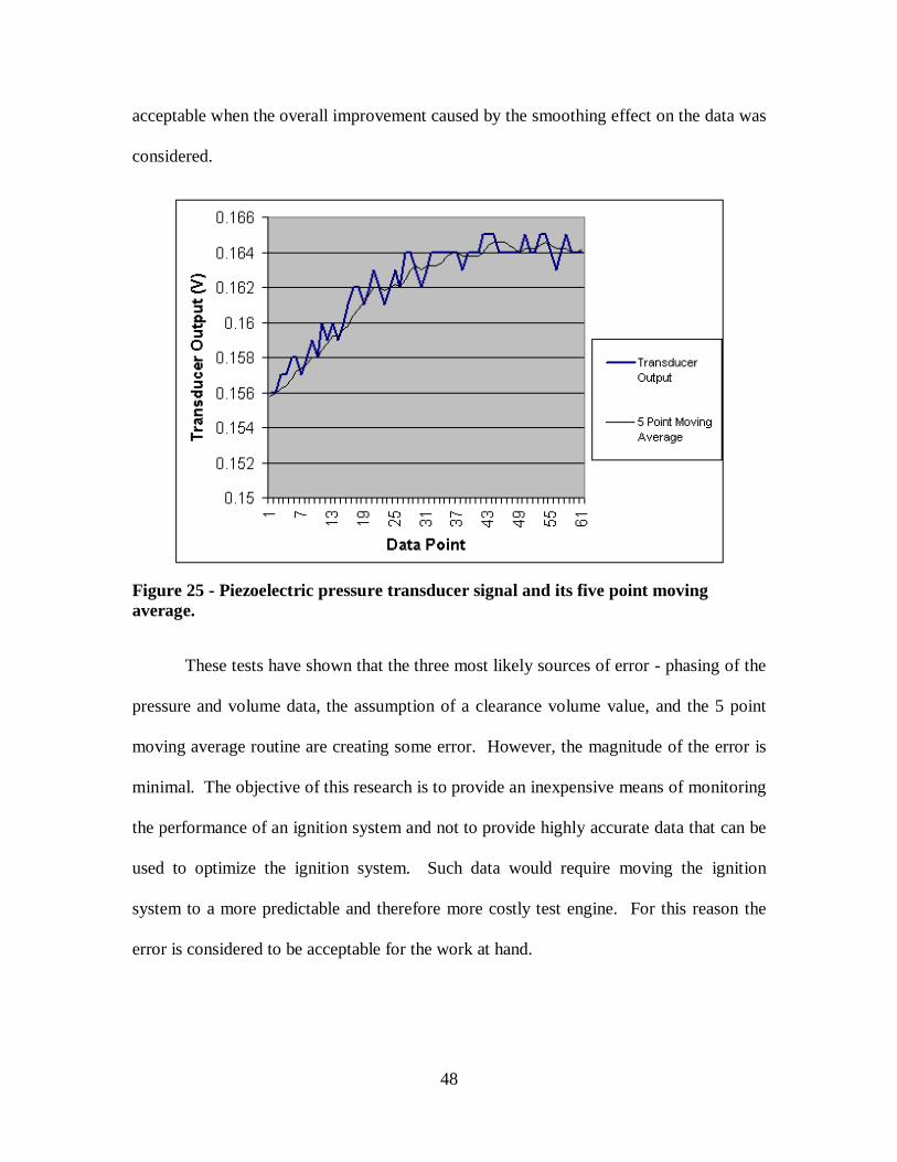
48
acceptable when the overall improvement caused by the smoothing effect on the data was
considered.
Figure 25 - Piezoelectric pressure transducer signal and its five point movingaverage.
These tests have shown that the three most likely sources of error - phasing of the
pressure and volume data, the assumption of a clearance volume value, and the 5 point
moving average routine are creating some error. However, the magnitude of the error is
minimal. The objective of this research is to provide an inexpensive means of monitoring
the performance of an ignition system and not to provide highly accurate data that can be
used to optimize the ignition system. Such data would require moving the ignition
system to a more predictable and therefore more costly test engine. For this reason the
error is considered to be acceptable for the work at hand.

49
Chapter 6 – Error Analysis
The test engine system is made up of several different transducers and acquisition
systems. The information supplied by these systems is used to determine the engine
performance quantifying parameters. Since it is desirable to know the accuracy of these
parameters, an error analysis was conducted for the system. Each component in the
system has an inherent inaccuracy associated with it. If these inaccuracies are known,
one can calculate the error in any value that is calculated using data supplied by these
components by using the equation:
n
na u
fu
u
fu
u
fuE
∂∂⋅∆++
∂∂⋅∆+
∂∂⋅∆= L
22
11 , (13)
where Ea is the absolute error, ∆un is the error in the measured quantity un, and f is the
function of the measured values, u1, u2, … un, to be calculated [26].
Equation 13 was first applied to Equations 10 and 11. These equations govern the
calculation of cylinder volume. For the error calculations, all length measurements are
considered to be accurate to within 0.01”, and the bore is considered to be accurate to
within 0.005”. These estimations were derived from information found in the operator’s
manual for the engine [16]. The other parameter used in Equations 10 and 11 is crank
angle. This measurement is made by the Accu-Coder Model 755A. As discussed earlier,
this instrument is accurate to within 0.36 degrees [20]. It should be noted that all data
collected by the data acquisition system is subject to a small error due to the 12 bit
system. This error is on the order of 0.02% and is considered negligible when compared
to the other sources of error. When the calculations were carried out for Equations 10

50
and 11, it was determined that the absolute errors in cylinder displacement and volume
are approximately 0.8% and 2.3%, respectively.
Knowing this, the error in indicated work was calculated by applying Equation 13
to Equation 1. Equation 1 involves the measured values of cylinder pressure and change
in volume. The cylinder pressure measurements were made by the PCB Model 112B11
pressure transducer. The manufacturer’s specifications for this device state that it has a
maximum error of ± 0.07 kPa [18]. However, the readings from the piezoelectric
transducer were baselined by using data collected from the Omega Model PX 126-015D-
V, which has an error of ± 3.5 kPa [19]. The error in cylinder volume has been
determined to be approximately 2.3%. By applying Equation 13, it was determined that
the absolute error in indicated work is approximately 3.1%.
The remainder of the performance quantifying parameters are derived from the
work; therefore, it can be concluded that any errors in their values are of similar
magnitude to the work error.
Another measured parameter that has the potential to be a substantial source of
error is the mass flow rate of the fuel. The error contained in this reading is largely due
to human error and is therefore difficult to quantify. These values are determined by
reading from a digital scale the fuel consumed in three minutes as shown on a stopwatch.
If care is taken when making these readings, it is felt that the error can be kept below a
value of ± 2 grams, or approximately 5%.
As stated in Chapter 5, the objective of this research is to provide an inexpensive
means of monitoring the performance of an ignition system and not to provide highly
accurate data that can be used to optimize the ignition system. Such data would require

51
moving the ignition system to a more predictable and therefore more costly test engine.
For this reason these errors are considered to be acceptable for the work at hand.
52
Chapter 7 – Analysis of Initial Test Results
To prove the reliability of the test engine, three different ignition sources were
tested. These ignition sources were three conventional sparkplugs. The first two plugs
were Champion model RC12YC as seen in Figure 26, which is the sparkplug
recommended by Briggs & Stratton Corp. for use in the Vanguard engine. The gap on
the first sparkplug was set to the manufacturer’s specification of 0.03”. For the second
model RC12YC sparkplug, the gap was set to 0.008”. The third sparkplug tested was a
Champion model J19LM as seen in Figure 26 with the gap set to 0.03”. This sparkplug
has the same thread size as the model RC12YC, but it is only long enough to extend half
way through the head, thereby not allowing it to protrude into the combustion chamber.
In addition, the heat range of this plug differs from that of the manufacturer’s
recommended plug. The model J19LM is a “colder” plug than the model RC12YC. This
means that the operating temperature of the electrode will be less than the temperature of
the “hotter” model RC12YC plug. The result of this cooler temperature will be that the
fuel in contact with the electrode may not be completely vaporized, resulting in a fouled
plug and poor combustion.

53
Figure 26 - The Champion model RC12YC (top) and model J19LM (bottom) thatwere used for initial testing.
With the engine coupled to the dynamometer, which provided an estimated one
horsepower load, data was taken with the engine running on each of the three different
sparkplugs at approximately 2700 RPM, which is in the center of the engine’s normal
operating range. The data was then processed through the Excel macros and Engine.m.
7.1 Test Results for Champion Model RC12YC with a 0 .03” Gap
The first sparkplug tested was the manufacturer recommended Champion model
RC12YC with the gap set to the recommended 0.03”. The complete results from this test
can be found in Appendix D. From the results of this test, an estimate of the expected
performance of the test engine was developed. The plot of pressure versus volume for
the cylinder when this plug was used, as shown in Figure 27, displays characteristics
typical to a properly operating internal combustion engine.

54
Figure 27 - A P-V diagram for the cylinder using the Champion model RC12YCwith a gap of 0.03” displaying proper combustion.
This shape is characterized by the smooth club shaped curve that is formed by the
compression and expansion strokes, shown in green. In addition to the pressure versus
volume diagram, the performance parameters for the engine were also calculated and are
displayed in Table 1.
Smooth Club Shape
Proper Combustion

55
Table 1 - Engine performance parameters for the Champion Model RC12YC with agap of 0.03".
PARAMETER VALUE UNIT
Average Engine Speed 2790 RPM
Fuel Consumption 15.05 g/min
Average Exhaust Temperature 806.7 Celsius
Average Gross Indicated Power 0.79 kW
Average Gross Indicated Specific FuelConsumption
573.96 g/kW*h
Average Gross Indicated Mean EffectivePressure
142.1 kPa
Average Gross Fuel ConversionEfficiency
14.4 %
In an effort to determine if these calculated values were reasonable, research was
conducted to find typical values for the parameters. From Heywood [2], it was
discovered that typical exhaust gas temperatures for spark ignition engines are
approximately 650 °C. The experimentally determined value of 806.7 °C seems to be
reasonably close to the expected value but is a bit high. The exact reason for this
deviation is uncertain. The readings were reproduced multiple times using a multitude of
different hardware. As discussed in Taylor [27], the accurate measurement of exhaust
gas temperature is nearly impossible; normally the temperatures obtained have only
comparative significance. Since the work here is only concerned with comparing the
temperatures in an effort to judge the performance of an ignition system, and not with
using the temperatures to calculate engine parameters, the inaccuracy is inconsequential.
In addition to typical exhaust temperatures, Heywood [2] also supplies typical best values
56
for brake specific fuel consumption and brake mean effective pressure. They are 350
g/kW*h and 900 kPa, respectively. These parameters are determined using brake power
and are representative of the most efficient engine performance. However, the work here
is concerned with indicated parameters and not brake parameters, and due to the low
loads on the engine during testing, the engine was not operating near peak efficiency.
Therefore, the only comparison that can be made is to check that the experimental results
are on the same order of magnitude as values taken from Heywood [2], which they are.
As previously stated, due to low loads during testing, the engine was not
operating near peak efficiency, which is evident in the calculated value for average gross
fuel conversion efficiency of 14.4%. According to Heywood [2], this value can reach up
to 96% in lean burning spark ignition engines.
7.2 Test Results for Champion Model RC12YC with a 0 .008” Gap
The next sparkplug to be tested was the Champion Model RC12YC with the gap
set to 0.008”. This is substantially less than the gap of 0.03”, which is recommended by
the manufacturer. The gap was reduced in an attempt to impair the performance of the
plug and thus create poor combustion. The pressure versus volume curve shown in
Figure 28 shows signs of this poor combustion. The shape formed by the compression
and expansion strokes is no longer that of a smooth club. Instead, it shows signs of
delayed combustion. Delayed combustion occurs when the flame front does not
propagate quickly after ignition, and hence the piston has already begun to move down
the bore when combustion occurs. This is characterized by the dramatic pressure
increase late in the expansion stroke resulting in the shape displayed in Figure 28.

57
Figure 28 - A P-V diagram for the cylinder using the Champion model RC12YCwith a gap of 0.008" displaying delayed combustion.
In addition to the poor combustion discussed above, the second test plug produced
an even greater ignition problem known as misfire. Misfire occurs when a fresh charge is
drawn into the engine and compressed but fails to ignite and is discharged from the
cylinder during the exhaust stroke. This results in loss of power and wasted fuel. The
characteristic P-V diagram of a misfire caused by the second test plug can be seen in
Figure 29.
Delayed Combustion

58
Figure 29 - A P-V diagram for the cylinder using the Champion model RC12YCwith a gap of 0.008" displaying a misfire.
When the performance parameters for the engine were calculated using the data
collected from the test engine while the second test plug was used, the results supported
the theories formulated from the P-V diagram analysis. These performance parameters
are displayed in Table 2.
Misfire

59
Table 2 - Engine performance parameters for the Champion Model RC12YC with agap of 0.008".
PARAMETER VALUE UNIT
Average Engine Speed 2607 RPM
Fuel Consumption 19.6 g/min
Average Exhaust Temperature 680.6 Celsius
Average Gross Indicated Power 0.66 kW
Average Gross Indicated Specific FuelConsumption
885.99 g/kW*h
Average Gross Indicated Mean EffectivePressure
127.25 kPa
Average Gross Fuel ConversionEfficiency
9.2 %
These values show that for approximately the same engine speed and load, the
fuel consumption increased while the power produced decreased. This is a result of the
misfire cycles together with poor combustion. The presence of misfire is also evident in
the average exhaust temperature, which dropped significantly from the value shown in
the previous test. This drop was due to the discharge of cool unburned mixture after each
misfire cycle.
7.3 Test Results for Champion Model J19LM with a 0 .03” Gap
The final test plug was the Champion model J19LM with a gap setting of 0.03”.
This plug has the same thread size as the model RC12YC, but it is not long enough to
extend into the combustion chamber. This increased the clearance volume of the cylinder
slightly. However, the difference was insignificant when compared to the total clearance
volume and the effects due to this change were deemed negligible. When the data

60
collected while the engine was run using this ignition source was compiled, it was clear
that this design also resulted in poor combustion. The plot of pressure versus volume for
this data set, shown in Figure 30, displays signs of both delayed and incomplete
combustion. This is characterized by the gradual pressure increase late in the expansion
cycle. The pressure waves that can be seen on the expansion stroke in Figure 30 are most
likely due to resonation in the cavity that is created by the plug not extending fully into
the combustion chamber.
Figure 30 - A P-V diagram for the cylinder using the Champion model J19LM witha gap of 0.03" displaying delayed and incomplete combustion.
The engine operation parameters that were calculated by Engine.m for this
ignition source, displayed in Table 3, support the theories stated above. The values show
that for approximately the same engine speed and loading, the power output shows a
significant decrease from the values calculated for the first two plugs. And this decrease
Pressure Waves

61
occurs with out any evidence of misfire. This shows that the overall combustion
resulting from an ignition source of this design is very poor. In addition, the fuel
consumption remains approximately equal to that of the first test, which results in the
very poor value for fuel conversion efficiency.
Table 3 - Engine performance parameters for the Champion Model J19LM with agap of 0.03”.
PARAMETER VALUE UNIT
Average Engine Speed 2663 RPM
Fuel Consumption 15.4 g/min
Average Exhaust Temperature 851.1 Celsius
Average Gross Indicated Power 0.48 kW
Average Gross Indicated Specific FuelConsumption
1109 g/kW*h
Average Gross Indicated Mean EffectivePressure
91 kPa
Average Gross Fuel ConversionEfficiency
8.6 %
The test results discussed in this chapter show that the test engine is capable of
quantifying the performance of an ignition system. The Champion model RC12YC with
a gap setting of 0.03” clearly outperforms the Champion model J19LM with the same gap
setting and the Champion model RC12YC with a gap setting of 0.008”.

62
Chapter 8 – Conclusions and Recommendations
The goal of this work was to develop a test engine onto which an ignition system
could be installed and subsequently tested. This system was to allow the analysis of the
combustion process, as well as support the determination of values that could be used to
quantify the engine performance under the given operating conditions.
This test engine has been developed, and its abilities and accuracy tested. The
hardware portion of this system utilizes a 16 horsepower Briggs & Stratton Vanguard
engine along with multiple pressure, position, and temperature transducers. The signals
from these transducers are collected and compiled using a variety of software packages
including Labview, Excel, and Matlab. It is felt that this engine is capable of accurately
meeting the requirements set forth by the goals of this research.
The location of a dynamometer that is suitable for loading the test engine is
encouraged. It is felt that cycle-to-cycle variations will decrease dramatically with
increased engine load, and this will undoubtedly increase the reliability of the
information supplied by the test system.

63
List of References
1. Cummins, Lyle C. Internal Fire, Warrendale, PA, Society of AutomotiveEngineers, Inc., 1989.
2. Heywood, John B. Internal Combustion Engine Fundamentals, New York, NY,McGraw-Hill Book Company, 1988.
3. Smith, James E. (Morgantown, WV); Craven, Robert M. (Morgantown, WV);VanVoorhies, Kurt L. (Morgantown, WV); Bonazza, Thomas J. (Fairmont, WV);U.S. patent number 5,361,737, November 8, 1994.
4. Stiles, Richard; Thompson, Gregory J. Smith, James E. “Investigation of a RadioFrequency Plasma Igniter for Possible Internal Combustion Engine Use,” Societyof Automotive Engineers Technical Paper No. 970071, International Congressand Exposition, Detroit, MI, February 24 – 27, 1997.
5. Amann, Charles A. “Classical Combustion Diagnostics for Engine Research,”Society of Automotive Engineers Technical Paper No. 850395, InternationalCongress and Exposition, Detroit, MI, February 25 – March 1, 1985.
6. Amann, Charles A. “Cylinder-Pressure Measurement and Its Use in EngineResearch,” Society of Automotive Engineers Technical Paper No. 852067,International Fuels and Lubricants Meeting and Exposition, Tulsa, OK,October 21 – 24, 1985.
7. The American Society of Mechanical Engineers, Measurement of IndicatedPower, New York, NY, The American Society of Mechanical Engineers, 1970.
8. Alyea, John W. “The Development and Evaluation of an Electronic IndicatedHorsepower Meter,” Society of Automotive Engineers Technical Paper No.690181, International Automotive Engineering Congress, Detroit, MI,January 13 – 17, 1969.
9. Brown, William L. “The Caterpillar imep Meter and Engine Friction,” Society ofAutomotive Engineers Technical Paper No. 730150, International AutomotiveEngineering Congress, Detroit, MI, January 8 – 12, 1973.
10. Schafer, H.J. Krull, O. and Maege, B. “Thermal Stress on a PiezoelectricPressure Transducer in the Combustion Chamber of an SI-Engine,” Society ofAutomotive Engineers Technical Paper No. 850375, International Congress andExposition, Detroit, MI, February 25 – March 1, 1985.

64
11. Randolph, Andrew L. “Methods of Processing Cylinder-Pressure TransducerSignals to Maximize Data Accuracy,” Society of Automotive Engineers TechnicalPaper No. 900170, International Congress and Exposition, Detroit, MI,February 26 – March 2, 1990.
12. Omega Engineering, Inc. The Temperature Handbook, Stamford, CT, 1995.
13. Department of Mechanical and Aerospace Engineering, West Virginia University,Morgantown, WV, http://www.cemr.wvu.edu/~englab/, December 1, 1998.
14. Superflow Corporation, Colorado Springs, CO, http://www.superflow.com,December 1, 1998.
15. Briggs & Stratton Corporation, Milwaukee, WI, http://www.briggsracing.com,December 1, 1998.
16. Briggs & Stratton Corporation. Operator/Owner Manual Model Series 290400,294400, 303400 & 350400, Milwaukee, WI, 1997.
17. PCB Piezotronics, Inc., Depew, NY, http://www.pcb.com,December 1, 1998.
18. PCB Piezotronics, Inc. Pressure Transducer Model 112B11 Operator’s Manual,Depew, NY, 1994.
19. Omega Engineering, Inc. The Pressure Strain and Force Handbook, Stamford,CT, 1990.
20. Encoder Products Company, Sandpoint, Idaho, http://www.encoderprod.com,December 1, 1998.
21. National Instruments, Instrumentation Catalogue, Austin, TX, 1998.
22. Labview, Vers. 5.0 (Windows 95), National Instruments, 1998.
23. Excel 97, Vers. 97 (Windows 95), Microsoft, 1996.
24. Matlab, Vers. 4.2c. (Windows 95), The Math Works Inc., 1994.
25. Traver, Michael L. “An Analysis of In-Cylinder Pressure Histories in a Bi-FuelEngine,” Masters Thesis, West Virginia University, Morgantown, WV, 1994.
26. Doebelin, Ernest O. Measurement Systems Application and Design, New York,NY, McGraw-Hill Publishing Company, 1990.

65
27. Taylor, Charles F. The Internal Combustion Engine in Theory and Practice,Cambridge, MA, The MIT Press, 1985.

66
Appendix A - Intra-Cylinder Engine Data Excel Macro
Sub engine()’’ engine Macro’ Macro recorded 9/3/98 by chambers’’ Keyboard Shortcut: Ctrl+e’ Application.Run "ATPVBAEN.XLA!Moveavg",ActiveSheet.Range("$A$1:$A$12000") _ , ActiveSheet.Range("$B:$B"), 5, False, False, False Range("B1001:B9000").Select Selection.Cut Range("D1").Select ActiveSheet.Paste Range("B9001:B12000").Select Selection.Cut Range("E1").Select ActiveSheet.Paste ChDir "C:\MATLAB42\bin" ActiveWorkbook.SaveAs FileName:="C:\MATLAB42\bin\eng.wk1",FileFormat:=xlWK1 _ , Password:="", CreateBackup:=FalseEnd Sub

67
Appendix B - Extra-Cylinder Engine Data Excel Macro
Sub engine2()’’ engine2 Macro’ Macro recorded 9/9/98 by chambers’’ Keyboard Shortcut: Ctrl+s’
Range("B62002").Select ActiveCell.FormulaR1C1 = "=AVERAGE(R[-62001]C:R[-2]C)" Range("C62002").Select ActiveCell.FormulaR1C1 = "=AVERAGE(R[-62001]C:R[-2]C)" Range("D62002").Select ActiveCell.FormulaR1C1 = "=AVERAGE(R[-62001]C:R[-2]C)" Range("B62002").Select Selection.Copy Range("A62002").Select Selection.PasteSpecial Paste:=xlValues, Operation:=xlNone, SkipBlanks:= _ False, Transpose:=False Range("C62002").Select Application.CutCopyMode = False Selection.Copy Range("A62003").Select Selection.PasteSpecial Paste:=xlValues, Operation:=xlNone, SkipBlanks:= _ False, Transpose:=False Range("D62002").Select Application.CutCopyMode = False Selection.Copy Range("A62004").Select Selection.PasteSpecial Paste:=xlValues, Operation:=xlNone, SkipBlanks:= _ False, Transpose:=False Columns("B:B").Select Application.CutCopyMode = False Selection.ClearContents Columns("C:C").Select Selection.ClearContents Columns("D:D").Select Selection.ClearContents Range("A8001:A15997").Select Selection.Cut Range("B1").Select

68
ActiveSheet.Paste Range("A62002:A62004").Select Selection.Copy Range("B7998").Select Selection.PasteSpecial Paste:=xlValues, Operation:=xlNone, SkipBlanks:= _ False, Transpose:=False Application.CutCopyMode = False ChDir "C:\MATLAB42\BIN" ActiveWorkbook.SaveAs FileName:="C:\MATLAB42\BIN\eng2.wk1", FileFormat:=_ xlWK1, Password:="", CreateBackup:=FalseEnd Sub

69
Appendix C - Engine.m
To be run on a Matlab platform.
% William J. Chambers% 5-8-98
% This is a program to create P-V diagrams and analyze the combustion efficiencyfor a four-stroke engine.
% *NOTE before running, open the intra-cylinder data file in Excel and hit Ctrl-e.% Then open the extra-cylinder data file in Excel and hit Ctrl-s.
clearclc
f = input(’What is the fuel consumption of the engine in grams per minute under thecurrent operating conditions? ’);fuel = f/2;
% INPUTS FROM SPREADSHEET FILES
rng1 = [0 0 5 8000];
data = wk1read(’eng’, 0, 0, rng1);
rng2 = [0 0 2 8000];
data2 = wk1read(’eng2’, 0, 0, rng2);
% To calculate the speed of the engine.%----------------------------------------------------------------------------
pulses(1:8000,1) = data2(1:8000,1);
pulses(8001:15997,1) = data2(1:7997,2);
counter1 = 1;

70
while pulses(counter1,1) < 1, counter1 = counter1 + 1;end pulse1 = counter1;
counter1 = counter1 + 100;
while pulses(counter1,1) < 1, counter1 = counter1 + 1;end pulse2 = counter1;
counter1 = counter1 + 100;
while pulses(counter1,1) < 1, counter1 = counter1 + 1;end pulse3 = counter1;
counter1 = counter1 + 100;
while pulses(counter1,1) < 1, counter1 = counter1 + 1;end pulse4 = counter1;
counter1 = counter1 + 100;
while pulses(counter1,1) < 1, counter1 = counter1 + 1;end pulse5 = counter1;
counter1 = counter1 + 100;
while pulses(counter1,1) < 1, counter1 = counter1 + 1;end pulse6 = counter1;
counter1 = counter1 + 100;
while pulses(counter1,1) < 1, counter1 = counter1 + 1;end pulse7 = counter1;
counter1 = counter1 + 100;
while pulses(counter1,1) < 1, counter1 = counter1 + 1;end pulse8 = counter1;

71
counter1 = counter1 + 100;
while pulses(counter1,1) < 1, counter1 = counter1 + 1;end pulse9 = counter1;
counter1 = counter1 + 100;
while pulses(counter1,1) < 1, counter1 = counter1 + 1;end pulse10 = counter1;
rpm1 = 62500*60/(pulse2-pulse1);rpm2 = 62500*60/(pulse3-pulse2);rpm3 = 62500*60/(pulse4-pulse3);rpm4 = 62500*60/(pulse5-pulse4);rpm5 = 62500*60/(pulse6-pulse5);rpm6 = 62500*60/(pulse7-pulse6);rpm7 = 62500*60/(pulse8-pulse7);rpm8 = 62500*60/(pulse9-pulse8);rpm9 = 62500*60/(pulse10-pulse9);
avgrpm = (rpm1+rpm2+rpm3+rpm4+rpm5+rpm6+rpm7+rpm8+rpm9)/9;
% The program will now determine the inlet pressure, inlet temperature, and exhausttemperature.
%---------------------------------------------------------------------------------------------------
ipress = abs(data2(7998,2));inletp = 14.7-(ipress*15/.123);
itemp = data2(7999,2);inlet =.226584602+24152.109*itemp+67233.4248*itemp^2+2210340.682*itemp^3-860963914.9*itemp^4+48350600000*itemp^5-1184520000000*itemp^6+13869000000000*itemp^7-63370800000000*itemp^8;

72
etemp = data2(8000,2);exhaust =.226584602+24152.109*etemp+67233.4248*etemp^2+2210340.682*etemp^3-860963914.9*etemp^4+48350600000*etemp^5-1184520000000*etemp^6+13869000000000*etemp^7-63370800000000*etemp^8;
% Forming the pressure matrix%----------------------------------------------------------------------------
p(1:8000,1) = data(1:8000,4);
p(8001:11000,1) = data(1:3000,5);
% To start the analysis at TDC on the intake stroke%----------------------------------------------------------------------------
if p(1,1) < p(1000,1) TDC1 = 1;
elseTDC1 = 1000;
end
TDC2 = TDC1 + 1000;TDC3 = TDC2 + 1000;TDC4 = TDC3 + 1000;TDC5 = TDC4 + 1000;TDC6 = TDC5 + 1000;TDC7 = TDC6 + 1000;TDC8 = TDC7 + 1000;TDC9 = TDC8 + 1000;TDC10 = TDC9 + 1000;TDC11 = TDC10 + 999;

73
% Now, the program will form the P-V diagrams to be plotted.%--------------------------------------------------------------------------------------------------
% To convert the pressure data to pressure units%---------------------------------------------------------------------------
constantp1 = TDC1+250;constantp2 = constantp1 + 1;constantp3 = constantp2 + 1;constantp4 = constantp3 + 1;constantp5 = constantp4 + 1;
zeroingp1 = (p(constantp1) + p(constantp2) + p(constantp3) + p(constantp4) +p(constantp5))/5;pressure1 = ((((p(TDC1:TDC3,1))-zeroingp1)*1000)/1.08216)+inletp;
constantp6 = TDC3+250;constantp7 = constantp6 + 1;constantp8 = constantp7 + 1;constantp9 = constantp8 + 1;constantp10 = constantp9 + 1;
zeroingp2 = (p(constantp6) + p(constantp7) + p(constantp8) + p(constantp9) +p(constantp10))/5;pressure2 = ((((p(TDC3:TDC5,1))-zeroingp2)*1000)/1.08216)+inletp;
constantp11 = TDC5+250;constantp12 = constantp11 + 1;constantp13 = constantp12 + 1;constantp14 = constantp13 + 1;constantp15 = constantp14 + 1;
zeroingp3 = (p(constantp11) + p(constantp12) + p(constantp13) + p(constantp14) +p(constantp15))/5;pressure3 = ((((p(TDC5:TDC7,1))-zeroingp3)*1000)/1.08216)+inletp;

74
constantp16 = TDC7+250;constantp17 = constantp16 + 1;constantp18 = constantp17 + 1;constantp19 = constantp18 + 1;constantp20 = constantp19 + 1;
zeroingp4 = (p(constantp16) + p(constantp17) + p(constantp18) + p(constantp19) +p(constantp20))/5;pressure4 = ((((p(TDC7:TDC9,1))-zeroingp4)*1000)/1.08216)+inletp;
constantp21 = TDC9+250;constantp22 = constantp21 + 1;constantp23 = constantp22 + 1;constantp24 = constantp23 + 1;constantp25 = constantp24 + 1;
zeroingp5 = (p(constantp21) + p(constantp22) + p(constantp23) + p(constantp24) +p(constantp25))/5;pressure5 = ((((p(TDC9:TDC11,1))-zeroingp5)*1000)/1.08216)+inletp;
% To convert the position data to volume units%----------------------------------------------------------------------------
% First we must form theta arrays from 0 to 4 pi radians in increments of2 pi/1000.
% To form the theta array for the first cycle.%----------------------------------------------------------------------------
array = [1:2000];
Theta1 = array’ * 2*pi/1000;
% To form the theta array for the second cycle.%----------------------------------------------------------------------------
Theta2 = array’ * 2*pi/1000;

75
% To form the theta array for the third cycle.%----------------------------------------------------------------------------
Theta3 = array’ * 2*pi/1000;
% To form the theta array for the fourth cycle.%----------------------------------------------------------------------------
Theta4 = array’ * 2*pi/1000;
% To form the theta array for the fifth cycle.%----------------------------------------------------------------------------
Theta5 = array’ * 2*pi/1000;
% The theta values must now be converted to volume units.%----------------------------------------------------------------------------
% Specifying the physical parameters of the test engine:
r = 1.3;l = 4.13;b = 2.68;clearanceV = 2.45;
% For the first cycle%----------------------------------
% From Heywood:
s = sin(Theta1);s2 = s.^2;

76
x = r * cos(Theta1) + sqrt(l^2 - (r^2 * s2));
volume1 = clearanceV + pi * (b/2)^2 * (l + r - x);
% For the second cycle%----------------------------------
s = sin(Theta2);s2 = s.^2;
x = r * cos(Theta2) + sqrt(l^2 - (r^2 * s2));
volume2 = clearanceV + pi * (b/2)^2 * (l + r - x);
% For the third cycle%----------------------------------
s = sin(Theta3);s2 = s.^2;
x = r * cos(Theta3) + sqrt(l^2 - (r^2 * s2));
volume3 = clearanceV + pi * (b/2)^2 * (l + r - x);
% For the fourth cycle%----------------------------------
s = sin(Theta4);s2 = s.^2;
x = r * cos(Theta4) + sqrt(l^2 - (r^2 * s2));
volume4 = clearanceV + pi * (b/2)^2 * (l + r - x);
% For the fifth cycle%----------------------------------
s = sin(Theta5);

77
s2 = s.^2;
x = r * cos(Theta5) + sqrt(l^2 - (r^2 * s2));
volume5 = clearanceV + pi * (b/2)^2 * (l + r - x);
% To create the arrays for the first cycle’s P-V diagram%-----------------------------------------------------------------------------
PRESSURE1a = pressure1(1:500,1);PRESSURE1b = pressure1(500:1000,1);PRESSURE1c = pressure1(1000:1500,1);
PRESSURE1d = pressure1(1500:2000,1);
VOLUME1a = volume1(1:500,1);VOLUME1b = volume1(500:1000,1);VOLUME1c = volume1(1000:1500,1);VOLUME1d = volume1(1500:2000,1);
% To create the arrays for the second cycle’s P-V diagram%-----------------------------------------------------------------------------
PRESSURE2a = pressure2(1:500,1);PRESSURE2b = pressure2(500:1000,1);PRESSURE2c = pressure2(1000:1500,1);PRESSURE2d = pressure2(1500:2000,1);
VOLUME2a = volume2(1:500,1);VOLUME2b = volume2(500:1000,1);VOLUME2c = volume2(1000:1500,1);VOLUME2d = volume2(1500:2000,1);
% To create the arrays for the third cycle’s P-V diagram%-----------------------------------------------------------------------------

78
PRESSURE3a = pressure3(1:500,1);PRESSURE3b = pressure3(500:1000,1);PRESSURE3c = pressure3(1000:1500,1);PRESSURE3d = pressure3(1500:2000,1);
VOLUME3a = volume3(1:500,1);VOLUME3b = volume3(500:1000,1);VOLUME3c = volume3(1000:1500,1);VOLUME3d = volume3(1500:2000,1);
% To create the arrays for the fourth cycle’s P-V diagram%-----------------------------------------------------------------------------
PRESSURE4a = pressure4(1:500,1);PRESSURE4b = pressure4(500:1000,1);PRESSURE4c = pressure4(1000:1500,1);PRESSURE4d = pressure4(1500:2000,1);
VOLUME4a = volume4(1:500,1);VOLUME4b = volume4(500:1000,1);VOLUME4c = volume4(1000:1500,1);VOLUME4d = volume4(1500:2000,1);
% To create the arrays for the fifth cycle’s P-V diagram%-----------------------------------------------------------------------------
PRESSURE5a = pressure5(1:500,1);PRESSURE5b = pressure5(500:1000,1);PRESSURE5c = pressure5(1000:1500,1);PRESSURE5d = pressure5(1500:2000,1);
VOLUME5a = volume5(1:500,1);VOLUME5b = volume5(500:1000,1);VOLUME5c = volume5(1000:1500,1);VOLUME5d = volume5(1500:2000,1);
% The program will now calculate the gross and net indicated work, and grosspower per cycle.
%--------------------------------------------------------------------------

79
% For cycle 1%---------------------------------------
A1a = abs(TRAPZ(PRESSURE1a,VOLUME1a));A1b = abs(TRAPZ(PRESSURE1b,VOLUME1b));A1c = abs(TRAPZ(PRESSURE1c,VOLUME1c));A1d = abs(TRAPZ(PRESSURE1d,VOLUME1d));
C1giw = (A1c - A1b);
C1niw = (A1c - A1b) - (A1d - A1a);
hp1 = avgrpm*C1giw/60/12/2/550;
p1metric = hp1*.7457;
% For cycle 2%---------------------------------------
A2a = abs(TRAPZ(PRESSURE2a,VOLUME2a));A2b = abs(TRAPZ(PRESSURE2b,VOLUME2b));A2c = abs(TRAPZ(PRESSURE2c,VOLUME2c));A2d = abs(TRAPZ(PRESSURE2d,VOLUME2d));
C2giw = (A2c - A2b);
C2niw = (A2c - A2b) - (A2d - A2a);
hp2 = avgrpm*C2giw/60/12/2/550;
p2metric = hp2*.7457;
% For cycle 3%---------------------------------------
A3a = abs(TRAPZ(PRESSURE3a,VOLUME3a));A3b = abs(TRAPZ(PRESSURE3b,VOLUME3b));A3c = abs(TRAPZ(PRESSURE3c,VOLUME3c));A3d = abs(TRAPZ(PRESSURE3d,VOLUME3d));
C3giw = (A3c - A3b);
C3niw = (A3c - A3b) - (A3d - A3a);

80
hp3 = avgrpm*C3giw/60/12/2/550;
p3metric = hp3*.7457;
% For cycle 4%---------------------------------------
A4a = abs(TRAPZ(PRESSURE4a,VOLUME4a));A4b = abs(TRAPZ(PRESSURE4b,VOLUME4b));A4c = abs(TRAPZ(PRESSURE4c,VOLUME4c));A4d = abs(TRAPZ(PRESSURE4d,VOLUME4d));
C4giw = (A4c - A4b);
C4niw = (A4c - A4b) - (A4d - A4a);
hp4 = avgrpm*C4giw/60/12/2/550;
p4metric = hp4*.7457;
% For cycle 5%---------------------------------------
A5a = abs(TRAPZ(PRESSURE5a,VOLUME5a));A5b = abs(TRAPZ(PRESSURE5b,VOLUME5b));A5c = abs(TRAPZ(PRESSURE5c,VOLUME5c));A5d = abs(TRAPZ(PRESSURE5d,VOLUME5d));
C5giw = (A5c - A5b);
C5niw = (A5c - A5b) - (A5d - A5a);
hp5 = avgrpm*C5giw/60/12/2/550;
p5metric = hp5*.7457;
avghp = (hp1+hp2+hp3+hp4+hp5)/5;
avgpmetric = avghp*.7457;

81
% The program will now calculate the gross isfc.%-------------------------------------------------------------------
C1isfc = fuel*60/p1metric;C2isfc = fuel*60/p2metric;C3isfc = fuel*60/p3metric;C4isfc = fuel*60/p4metric;C5isfc = fuel*60/p5metric;
avgisfc = fuel*60/avgpmetric;
% The program will now calculate the gross imep.%-------------------------------------------------------------------
C1imep = hp1*2*396000/14.65/avgrpm*6.895;C2imep = hp2*2*396000/14.65/avgrpm*6.895;C3imep = hp3*2*396000/14.65/avgrpm*6.895;C4imep = hp4*2*396000/14.65/avgrpm*6.895;C5imep = hp5*2*396000/14.65/avgrpm*6.895;
avgimep = (C1imep+C2imep+C3imep+C4imep+C5imep)/5;
% The program will now calculate the average fuel conversion efficiency.%-------------------------------------------------------------------
flow = fuel*60;
C1fce = 3600/(flow*44/p1metric)*100;C2fce = 3600/(flow*44/p2metric)*100;C3fce = 3600/(flow*44/p3metric)*100;C4fce = 3600/(flow*44/p4metric)*100;C5fce = 3600/(flow*44/p5metric)*100;
avgfce = 3600/(flow*44/avgpmetric)*100;
% The program will now display the calculated values.%-------------------------------------------------------------------space = ’ ’;

82
disp(space)disp(space)disp(space)disp(space)disp(space)disp(space)disp(space)disp(space)disp(space)disp(space)disp(space)disp(space)disp(space)disp(space)stat = ’ The average speed of the engine in RPM is:’;disp(stat)disp(space)disp(avgrpm)disp(space)stat1 = ’ The average exhaust temperature of the engine in degrees Celsius is:’;disp(space)disp(stat1)disp(space)disp(exhaust)disp(space)disp(space)
stat2 = ’ The gross indicated power of the cylinder in (kW) for each cycle is asfollows.’;disp(stat2)disp(space)
stat3 = ’Cycle One:’;disp(stat3)disp(space)disp(p1metric)disp(space)
stat4 = ’Cycle Two:’;disp(stat4)disp(space)disp(p2metric)disp(space)
stat5 = ’Cycle Three:’;disp(stat5)

83
disp(space)disp(p3metric)disp(space)
stat6 = ’Cycle Four:’;disp(stat6)disp(space)disp(p4metric)disp(space)
stat7 = ’Cycle Five:’;disp(stat7)disp(space)disp(p5metric)disp(space)
stat8 = ’ The average gross indicated power of the cylinder in (kW) is:’;disp(stat8)disp(space)disp(avgpmetric)
disp(space)disp(space)disp(space)stat9 = ’ The gross indicated specific fuel consumption of the cylinder in (g/kW*h)for each cycle is as follows.’;disp(stat9)disp(space)
stat10 = ’Cycle One:’;disp(stat10)disp(space)disp(C1isfc)disp(space)
stat11 = ’Cycle Two:’;disp(stat11)disp(space)disp(C2isfc)disp(space)
stat12 = ’Cycle Three:’;disp(stat12)disp(space)disp(C3isfc)

84
disp(space)
stat13 = ’Cycle Four:’;disp(stat13)disp(space)disp(C4isfc)disp(space)
stat14 = ’Cycle Five:’;disp(stat14)disp(space)disp(C5isfc)disp(space)
stat15 = ’ The average gross indicated specific fuel consumption of the cylinder in(g/kW*h) is:’;disp(stat15)disp(space)disp(avgisfc)
disp(space)disp(space)disp(space)stat16 = ’ The gross indicated mean effective pressure of the cylinder in (kPa) foreach cycle is as follows.’;disp(stat16)disp(space)
stat17 = ’Cycle One:’;disp(stat17)disp(space)disp(C1imep)disp(space)
stat18 = ’Cycle Two:’;disp(stat18)disp(space)disp(C2imep)disp(space)
stat19 = ’Cycle Three:’;disp(stat19)disp(space)disp(C3imep)disp(space)

85
stat20 = ’Cycle Four:’;disp(stat20)disp(space)disp(C4imep)disp(space)
stat21 = ’Cycle Five:’;disp(stat21)disp(space)disp(C5imep)disp(space)
stat22 = ’ The average gross indicated mean effective pressure of the cylinder in(kPa) is:’;disp(stat22)disp(space)disp(avgimep)disp(space)disp(space)disp(space)
stat23 = ’ The percent fuel conversion efficiency of the cylinder for each cycle is asfollows.’;disp(stat23)disp(space)
stat24 = ’Cycle One:’;disp(stat24)disp(space)disp(C1fce)disp(space)
stat25 = ’Cycle Two:’;disp(stat25)disp(space)disp(C2fce)disp(space)
stat26 = ’Cycle Three:’;disp(stat26)disp(space)disp(C3fce)disp(space)
stat27 = ’Cycle Four:’;disp(stat27)

86
disp(space)disp(C4fce)disp(space)
stat28 = ’Cycle Five:’;disp(stat28)disp(space)disp(C5fce)disp(space)
stat29 = ’ The average percent gross fuel conversion efficiency for the cylinder is:’;disp(stat29)disp(space)disp(avgfce)
% To create the first cycle’s PV Diagram:%-------------------------------------------------------------------
d = MENU(’Would you like to see a P-V diagram for the first cycle?’,’YES’,’NO’);
if d == 1,plot(VOLUME1a/16.12,PRESSURE1a/inletp,’r-’);axis([0 1.1 0 35])axis(axis)title(’P-V Diagram for Cycle 1’)xlabel(’Cylinder Volume / Maximum Volume’)ylabel(’Cylinder Pressure / Intake Pressure’)hold onplot(VOLUME1b/16.12,PRESSURE1b/inletp,’g-’);plot(VOLUME1c/16.12,PRESSURE1c/inletp,’g-’);plot(VOLUME1d/16.12,PRESSURE1d/inletp,’r-’);hold off
end
% To create the second cycle’s P-V Diagram:%-------------------------------------------------------------------
d2 = MENU(’Would you like to see a P-V diagram for the second cycle?’,’YES’,’NO’);
if d2 == 1,plot(VOLUME2a/16.12,PRESSURE2a/inletp,’r-’);axis([0 1.1 0 35])axis(axis)

87
title(’P-V Diagram for Cycle 2’)xlabel(’Cylinder Volume / Maximum Volume’)ylabel(’Cylinder Pressure / Intake Pressure’)hold onplot(VOLUME2b/16.12,PRESSURE2b/inletp,’g-’);plot(VOLUME2c/16.12,PRESSURE2c/inletp,’g-’);plot(VOLUME2d/16.12,PRESSURE2d/inletp,’r-’);hold off
end
% To create the third cycle’s P-V Diagram:%-------------------------------------------------------------------
d3 = MENU(’Would you like to see a P-V diagram for the third cycle?’,’YES’,’NO’);
if d3 == 1,plot(VOLUME3a/16.12,PRESSURE3a/inletp,’r-’);axis([0 1.1 0 35])axis(axis)title(’P-V Diagram for Cycle 3’)xlabel(’Cylinder Volume / Maximum Volume’)ylabel(’Cylinder Pressure / Intake Pressure’)hold onplot(VOLUME3b/16.12,PRESSURE3b/inletp,’g-’);plot(VOLUME3c/16.12,PRESSURE3c/inletp,’g-’);plot(VOLUME3d/16.12,PRESSURE3d/inletp,’r-’);hold off
end
% To create the fourth cycle’s P-V Diagram:%-------------------------------------------------------------------
d4 = MENU(’Would you like to see a P-V diagram for the fourth cycle?’,’YES’,’NO’);
if d4 == 1,plot(VOLUME4a/16.12,PRESSURE4a/inletp,’r-’);axis([0 1.1 0 35])axis(axis)title(’P-V Diagram for Cycle 4’)xlabel(’Cylinder Volume / Maximum Volume)’)ylabel(’Cylinder Pressure / Intake Pressure’)hold on

88
plot(VOLUME4b/16.12,PRESSURE4b/inletp,’g-’);plot(VOLUME4c/16.12,PRESSURE4c/inletp,’g-’);plot(VOLUME4d/16.12,PRESSURE4d/inletp,’r-’);hold off
end
% To create the fifth cycle’s P-V Diagram:%-------------------------------------------------------------------
d5 = MENU(’Would you like to see a P-V diagram for the fifth cycle?’,’YES’,’NO’);
if d5 == 1,plot(VOLUME5a/16.12,PRESSURE5a/inletp,’r-’);axis([0 1.1 0 35])axis(axis)title(’P-V Diagram for Cycle 5’)xlabel(’Cylinder Volume / Maximum Volume’)ylabel(’Cylinder Pressure / Intake Pressure’)hold onplot(VOLUME5b/16.12,PRESSURE5b/inletp,’g-’);plot(VOLUME5c/16.12,PRESSURE5c/inletp,’g-’);plot(VOLUME5d/16.12,PRESSURE5d/inletp,’r-’);hold off
end
89
Appendix D - Output of Engine.m for the Champion Model RC12YCSparkplug with the Recommended Gap of .03”
What is the fuel consumption of the engine in grams per minute under the current
operating conditions? 15.05
The average speed of the engine in RPM is:
2.7904e+003
The average exhaust temperature of the engine in degrees Celsius is:
806.7166
The gross indicated power of the cylinder in (kW) for each cycle is as follows.
Cycle One:
0.7234
Cycle Two:
0.8198
Cycle Three:

90
0.7287
Cycle Four:
0.7681
Cycle Five:
0.9261
The average gross indicated power of the cylinder in (kW) is:
0.7932
The gross indicated specific fuel consumption of the cylinder in (g/kW*h) for each cycle
is as follows.
Cycle One:
624.1563
Cycle Two:
550.7438
Cycle Three:
619.6110
Cycle Four:
587.7845
Cycle Five:

91
487.5233
The average gross indicated specific fuel consumption of the cylinder in (g/kW*h) is:
573.9638
The gross indicated mean effective pressure of the cylinder in (kPa) for each cycle is as
follows.
Cycle One:
129.5848
Cycle Two:
146.8581
Cycle Three:
130.5354
Cycle Four:
137.6034
Cycle Five:
165.9022
The average gross indicated mean effective pressure of the cylinder in (kPa) is:

92
142.0968
The percent gross fuel conversion efficiency of the cylinder for each cycle is as follows.
Cycle One:
13.1086
Cycle Two:
14.8559
Cycle Three:
13.2048
Cycle Four:
13.9198
Cycle Five:
16.7824
The average percent gross fuel conversion efficiency for the cylinder is:
14.3743

93
Figure D 1 – Pressure versus volume diagram for cycle one using the Championmodel RC12YC sparkplug with the recommended gap of 0.03”
Figure D 2 - Pressure versus volume diagram for cycle two using the Championmodel RC12YC sparkplug with the recommended gap of 0.03”

94
Figure D 3 - Pressure versus volume diagram for cycle three using the Championmodel RC12YC sparkplug with the recommended gap of 0.03”
Figure D 4 - Pressure versus volume diagram for cycle four using the Championmodel RC12YC sparkplug with the recommended gap of 0.03”

95
Figure D 5 - Pressure versus volume diagram for cycle five using the Championmodel RC12YC sparkplug with the recommended gap of 0.03”

96
Appendix E - Output of Engine.m for the Champion Model RC12YCSparkplug with a Gap of .008”
What is the fuel consumption of the engine in grams per minute under the current
operating conditions? 19.6
The average speed of the engine in RPM is:
2.6070e+003
The average exhaust temperature of the engine in degrees Celsius is:
680.5703
The gross indicated power of the cylinder in (kW) for each cycle is as follows.
Cycle One:
1.1011
Cycle Two:
1.2186
Cycle Three:

97
1.1338
Cycle Four:
-0.0974
Cycle Five:
-0.0378
The average gross indicated power of the cylinder in (kW) is:
0.6637
The gross indicated specific fuel consumption of the cylinder in (g/kW*h) for each cycle
is as follows.
Cycle One:
534.0048
Cycle Two:
482.5266
Cycle Three:
518.6245
Cycle Four:
-6.0369e+003
Cycle Five:
98
-1.5576e+004
The average gross indicated specific fuel consumption of the cylinder in (g/kW*h) is:
885.9916
The gross indicated mean effective pressure of the cylinder in (kPa) for each cycle is as
follows.
Cycle One:
211.1287
Cycle Two:
233.6528
Cycle Three:
217.3899
Cycle Four:
-18.6757
Cycle Five:
-7.2384
The average gross indicated mean effective pressure of the cylinder in (kPa) is:

99
127.2515
The percent fuel conversion efficiency of the cylinder for each cycle is as follows.
Cycle One:
15.3216
Cycle Two:
16.9562
Cycle Three:
15.7760
Cycle Four:
-1.3553
Cycle Five:
-0.5253
The average percent gross fuel conversion efficiency for the cylinder is:
9.2346

100
Figure E 1 - Pressure versus volume diagram for cycle one using the Championmodel RC12YC sparkplug with a gap of 0.008”
Figure E 2 - Pressure versus volume diagram for cycle two using the Championmodel RC12YC sparkplug with a gap of 0.008”

101
Figure E 3 - Pressure versus volume diagram for cycle three using the Championmodel RC12YC sparkplug with a gap of 0.008”
Figure E 4 - Pressure versus volume diagram for cycle four using the Championmodel RC12YC sparkplug with a gap of 0.008”

102
Figure E 5 - Pressure versus volume diagram for cycle five using the Championmodel RC12YC sparkplug with a gap of 0.008”

103
Appendix F - Output of Engine.m for the Champion Model J19LMSparkplug with a .03” Gap.
What is the fuel consumption of the engine in grams per minute under the current
operating conditions? 15.4
The average speed of the engine in RPM is:
2.6627e+003
The average exhaust temperature of the engine in degrees Celsius is:
851.1185
The gross indicated power of the cylinder in (kW) for each cycle is as follows.
Cycle One:
0.5258
Cycle Two:
0.6227
Cycle Three:

104
0.5756
Cycle Four:
0.2127
Cycle Five:
0.4872
The average gross indicated power of the cylinder in (kW) is:
0.4848
The gross indicated specific fuel consumption of the cylinder in (g/kW*h) for each cycle
is as follows.
Cycle One:
878.7269
Cycle Two:
741.9529
Cycle Three:
802.5948
Cycle Four:
2.1720e+003
Cycle Five:

105
948.3324
The average gross indicated specific fuel consumption of the cylinder in (g/kW*h) is:
1.1087e+003
The gross indicated mean effective pressure of the cylinder in (kPa) for each cycle is as
follows.
Cycle One:
98.7006
Cycle Two:
116.8954
Cycle Three:
108.0631
Cycle Four:
39.9314
Cycle Five:
91.4562
The average gross indicated mean effective pressure of the cylinder in (kPa) is:
106
91.0094
The percent fuel conversion efficiency of the cylinder for each cycle is as follows.
Cycle One:
9.3110
Cycle Two:
11.0274
Cycle Three:
10.1942
Cycle Four:
3.7670
Cycle Five:
8.6276
The average percent gross fuel conversion efficiency for the cylinder is:
8.5854

107
Figure F 1 - Pressure versus volume diagram for cycle one using the Championmodel J19LM sparkplug with a 0.03” gap.
Figure F 2 - Pressure versus volume diagram for cycle two using the Championmodel J19LM sparkplug with a 0.03” gap.

108
Figure F 3 - Pressure versus volume diagram for cycle three using the Championmodel J19LM sparkplug with a 0.03” gap.
Figure F 4 - Pressure versus volume diagram for cycle four using the Championmodel J19LM sparkplug with a 0.03” gap.

109
Figure F 5 - Pressure versus volume diagram for cycle five using the Championmodel J19LM sparkplug with a 0.03” gap.

110
Approval of Examining Committee
____________________________________Nigel N. Clark, Ph.D.
____________________________________James E. Smith, Ph.D.
_____________ ____________________________________Date Gregory J. Thompson, Ph.D., Chairman