enes witwit university of heidelberg may 10, 2017 · enes witwit university of heidelberg may 10,...
TRANSCRIPT

Deep Learning Speech Recognition
Enes WitwitUniversity of Heidelberg
May 10, 2017

Contents
1 Introduction
2 Architecture
3 Preprocessing
4 Decoding
5 Concluding Remarks

1 Introduction
2 Architecture
3 Preprocessing
4 Decoding
5 Concluding Remarks

Introduction
Automatic Speech Recognition (ASR)
Definition Automatic transformation of spoken language byhumans into the corresponding word sequence.
1 / 59
Introduction
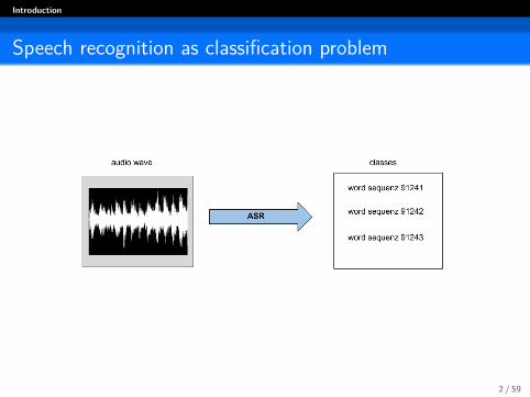
Speech recognition as classification problem
Figure: ASR as classification problem
2 / 59

Introduction
ASR Applications
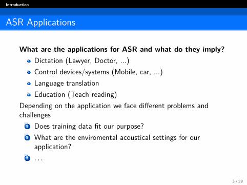
What are the applications for ASR and what do they imply?Dictation (Lawyer, Doctor, ...)Control devices/systems (Mobile, car, ...)Language translationEducation (Teach reading)
Depending on the application we face different problems andchallenges
1 Does training data fit our purpose?2 What are the enviromental acoustical settings for our
application?3 . . .
3 / 59
Introduction
ASR Applications
What are the applications for ASR and what do they imply?Dictation (Lawyer, Doctor, ...)Control devices/systems (Mobile, car, ...)Language translationEducation (Teach reading)
Depending on the application we face different problems andchallenges
1 Does training data fit our purpose?2 What are the enviromental acoustical settings for our
application?3 . . .
3 / 59

Introduction
ASR Advantages
SpeedKeyboard 200-1000 characters per minuteSpeech 1000-4000 characters per minute
No need of using hands or eyesCommunication with systems/devices naturallyPortable
4 / 59

Introduction
ASR Disadvantages
Locational requirementsNot usable in locations where silence is requiredNot usable in loudy enviroments
Error rate still to high
5 / 59

Introduction
Difficulties
Variability
6 / 59
Introduction
Difficulties
Variability
6 / 59

Introduction
Difficulties
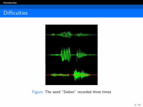
Size Number of word types in vocabularySpeaker speaker-independency, adaptation tospeaker characteristics and accentAcoustic environment Noise, competing speakers,channel conditions (microphone, phone line, roomacoustics)Style Planned monologue or spontaneousconversation.Continuous or isolated speech.
7 / 59
Introduction
Difficulties
Figure: The word ”Sieben” recorded three times
8 / 59
Introduction
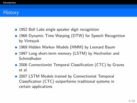
History
1952 Bell Labs single speaker digit recognition1968 Dynamic Time Warping (DTW) for Speech Recognitionby Vintsyuk1969 Hidden Markov Models (HMM) by Leonard Baum1997 Long short-term memory (LSTM) by Hochreiter andSchmidhuber2006 Connectionist Temporal Classification (CTC) by Graveset al.2007 LSTM Models trained by Connectionist TemporalClassification (CTC) outperforms traditional systems incertain applications
9 / 59
1 Introduction
2 Architecture
3 Preprocessing
4 Decoding
5 Concluding Remarks

Architecture
Standard ASR Pipeline
Figure: ASR Pipeline
10 / 59

1 Introduction
2 Architecture
3 Preprocessing
4 Decoding
5 Concluding Remarks

Preprocessing
Why do we need signal processing?
Need a form of signal we can work with easilyExtract relevant informationFilter unnecessary information
Speaker-dependent informationAcoustical enviromentMicrofon
Reduction of data size
11 / 59

Preprocessing
Spectogram
Figure: Deep Learning School 2016 (Talk: Adam Cotes, Baidu)
12 / 59

Preprocessing
Spectogram
Figure: Deep Learning School 2016 (Talk: Adam Cotes, Baidu)
13 / 59

Preprocessing
Mel Frequency Cepstral Coefficients(MFCC)
14 / 59

Preprocessing
Make signal processing intelligent again
Using audio wave as raw input for model trainingSainath et al., Interspeech 2015
15 / 59

1 Introduction
2 Architecture
3 Preprocessing
4 Decoding
5 Concluding Remarks
DecodingAcoustic Model
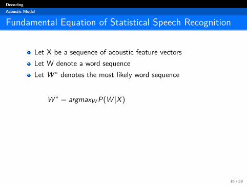
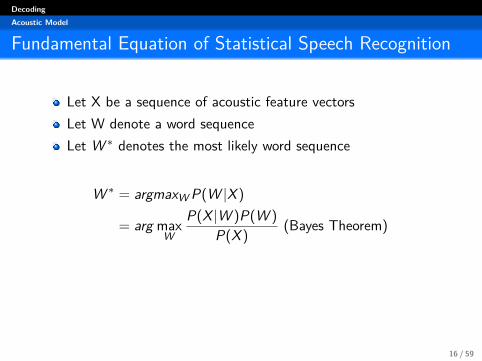
Fundamental Equation of Statistical Speech Recognition
Let X be a sequence of acoustic feature vectorsLet W denote a word sequenceLet W ∗ denotes the most likely word sequence
W ∗ = argmaxW P(W |X )
= arg maxW
P(X |W )P(W )P(X ) (Bayes Theorem)
= arg maxW
P(X |W )︸ ︷︷ ︸Acoustic model
P(W )︸ ︷︷ ︸Language Model
16 / 59
DecodingAcoustic Model
Fundamental Equation of Statistical Speech Recognition
Let X be a sequence of acoustic feature vectorsLet W denote a word sequenceLet W ∗ denotes the most likely word sequence
W ∗ = argmaxW P(W |X )
= arg maxW
P(X |W )P(W )P(X ) (Bayes Theorem)
= arg maxW
P(X |W )︸ ︷︷ ︸Acoustic model
P(W )︸ ︷︷ ︸Language Model
16 / 59

DecodingAcoustic Model
Approach
There are two approaches for developing an acoustic model1 Hidden Markov Model2 Neural Networks
17 / 59

DecodingAcoustic Model
Stochastic process
Definition (Markov chain of order n)
P(Xt+1 = st+1|Xt = st , . . . ,X0 = s0)= P(Xt+1 = st+1|Xt = st , . . . ,Xt−n+1 = st−n+1)
18 / 59

DecodingAcoustic Model
Hidden Markov Model (HMM)Suppose you cannot observe the states .
Figure: A Tutorial on Hidden Markov Models by Rabiner
19 / 59
DecodingAcoustic Model
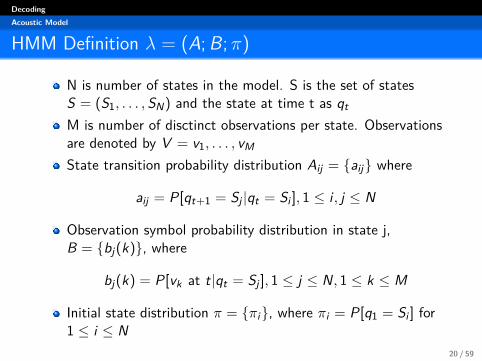
HMM Definition λ = (A; B; π)
N is number of states in the model. S is the set of statesS = (S1, . . . ,SN) and the state at time t as qt
M is number of disctinct observations per state. Observationsare denoted by V = v1, . . . , vM
State transition probability distribution Aij = {aij} where
aij = P[qt+1 = Sj |qt = Si ], 1 ≤ i , j ≤ N
Observation symbol probability distribution in state j,B = {bj(k)}, where
bj(k) = P[vk at t|qt = Sj ], 1 ≤ j ≤ N, 1 ≤ k ≤ M
Initial state distribution π = {πi}, where πi = P[q1 = Si ] for1 ≤ i ≤ N
20 / 59

DecodingAcoustic Model
HMM Assumptions
Figure: Probabilistic finite state automaton (Renals and Bell, ASRLecture, Edinburgh)
1 Observation independence An acoustic observation x isconditionally independent of all other observations given thestate that generated it
2 Markov process A state is conditionally independent of allother states given the previous state
21 / 59

DecodingAcoustic Model
Output Distribution
Figure: Probabilistic finite state automaton (Renals and Bell, ASRLecture, Edinburgh)
bj(x) = p(x |sj) = N (x ;µj ,Σj) (Single multivariate Gaussian)bj(x) = p(x |sj) =
∑Mm=1 cjmN (x ;µjm,Σjm) (M-component
Gaussian Mixture Model)
22 / 59

DecodingAcoustic Model
The three HMM Challenges
1 Evaluation Given a HMM λ, an Output O → What is theprobabilty that O is an Output of the HMM λ: P(O|λ)?Forward or Backward Algorithm
2 Decoding Given a HMM λ, an Output O. Find a sequence ofStates S = sj1, . . . , sjT for which holds S = argmaxSP(S,O|λ)Viterbi Algorithm
3 Training Given a HMM λ and a set of Training Data O. Findbetter Parameters λ′ such that P(O|λ) < P(O|λ′)Baum Welch Algorithm
23 / 59

DecodingAcoustic Model
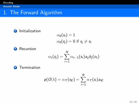
1. The Forward Algorithm
Goal Estimate P(O|λ)We need to sum over all possible state sequencess1, s2, . . . , sT that could result in the observation sequence ORather than enumerating each sequence, compute theprobabilities recursively (exploit the Markov Assumption)Forward Probability αt(sj):the probability of observing theobservation sequence o1, . . . , ot and being in state sj at time t:
at(sj) = p(x1, . . . , xt , S(t) = sj |λ)
24 / 59
DecodingAcoustic Model
1. The Forward Algorithm
1 Initializationα0(sl ) = 1α0(sj) = 0 if sj 6= sl
2 Recursion
αt(sj) =N∑
i=1αt−1(si )aijbj(ot)
3 Termination
p(O|λ) = αT (sE ) =N∑
i=1αT (si )aiE
25 / 59

DecodingAcoustic Model
Forward Recursion
26 / 59

DecodingAcoustic Model
1. The Backward Algorithm
1 InitializationβT (i) = 1 , 1 ≤ i ≤ |S|
2 Recursion
βt(i) =|S|∑j=1
βj(ot+1)aijβt+1(j) , 1 ≤ i ≤ |S| , 1 ≤ t < T
3 Termination
p(O|λ) =|S|∑j=1
πjbj(o1)β1(j)
27 / 59

DecodingAcoustic Model
Viterbi approximation
Instead of summing over all possible state sequences wechange the summation to a maximation in the recursion
Vt(sj) = maxiVt−1(si )aijbj(xt)
This change in the recursion gives us now the most probablepathWe need to keep track of the states that make up this path bykeeping a sequence of backpointers to enable a Viterbibacktrace: the backpointer for each state at each timeindicates the previous state on the most probable path
28 / 59

DecodingAcoustic Model
Viterbi approximation
29 / 59

DecodingAcoustic Model
Viterbi approximation
30 / 59

DecodingAcoustic Model
2.Decoding: The Viterbi Algorithm
1 InitializationV0(sl ) = 1V0(sj) = 0 if sj 6= sl
bt0(sj) = 02 Recursion
Vt(sj) = Nmaxi=1
Vt−1(si )aijbj(ot)
btt(sj) = arg Nmaxi=1
Vt−1(si )aijbj(ot)
3 Termination
P∗ = VT (sE ) = Nmaxi=1
VT (si )aiE
s∗T = btT (qE ) = arg Nmaxi=1
VT (si )aiE
31 / 59

DecodingAcoustic Model
Viterbi Backtrace
32 / 59

DecodingAcoustic Model
3.Training:Baum-Welch Algorithm
1 Forwad procedureLet αi (t) = P(Y1 = y1, ...,Yt = yt ,Xt = i |θ), the probabilityof seeing the y1, y2, ..., yt and being in state i at time t.
2 Backward procedureLet βi (t) = P(Yt+1 = yt+1, ...,YT = yT |Xt = i , θ) that is theprobability of the ending partial sequence yt+1, ..., yT givenstarting state i at time t.
3 Update
γi (t) = P(Xt = i |Y , θ) = αi (t)βi (t)∑Nj=1 αj(t)βj(t)
ξij(t) = P(Xt = i ,Xt+1 = j |Y , θ) = αi (t)aijβj(t + 1)bj(yt+1)∑Ni=1
∑Nj=1 αi (t)aijβj(t + 1)bj(yt+1)
33 / 59

DecodingAcoustic Model
3.Training:Baum-Welch Algorithm
Update parameters
π∗i = γi (1)
a∗ij =∑T−1
t=1 ξij(t)∑T−1t=1 γi (t)
b∗i (vk) =∑T
t=1 1yt=vkγi (t)∑Tt=1 γi (t)
34 / 59

DecodingAcoustic Model
Neural networks for acoustic models
Goal create a neural network (DNN/RNN) from which we canextract transcription y. Train with labeled pairs (x , y∗).
Figure: Deep Learning School 2016 (Adam Cotes, Baidu)
35 / 59

DecodingAcoustic Model
Recurrent Neural Network (RNN)
Figure: http://colah.github.io/posts/2015-09-NN-Types-FP/
36 / 59

DecodingAcoustic Model
Recurrent Neural Network (RNN)
Figure: http://colah.github.io/posts/2015-09-NN-Types-FP/
Forward propagation
hi = σ(Whhhi−1 + Whxxi + bh)yi = Wyhhi
37 / 59

DecodingAcoustic Model
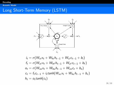
Long Short-Term Memory (LSTM)
Figure: Long Short-term Memory Cell from Graves et al. 2013
38 / 59
DecodingAcoustic Model
Long Short-Term Memory (LSTM)
it = σ(Wxixt + Whiht−1 + Wcict−1 + bi )ft = σ(Wxf xt + Whf ht−1 + Wcf ct−1 + bf )ot = σ(Wxoxt + Whoht−1 + Wcoct + bo)ct = ftct−1 + ittanh(Wxcxt + Whcht−1 + bc)ht = ottanh(ct)
39 / 59

DecodingAcoustic Model
Bidirectional RNN (BRNN)
Figure: http://colah.github.io/posts/2015-09-NN-Types-FP/
40 / 59

DecodingAcoustic Model
Train acoustic model
Main issue length(x) 6= length(y)Solution
Connectionist Temporal Classification [Graves et al., 2006]Attention, Sequence to Sequence
41 / 59

DecodingAcoustic Model
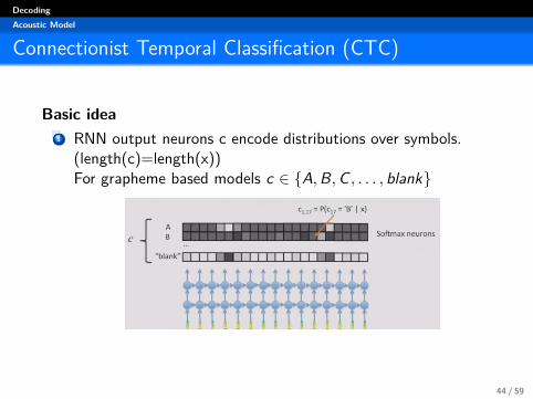
Connectionist Temporal Classification (CTC)
Basic idea1 RNN output neurons c encode distributions over symbols.
(length(c)=length(x))For phoneme based modelsc ∈ {AA,AE ,AX , . . . ,ER1, blank}For grapheme based models c ∈ {A,B,C , . . . , blank}
2 Define mapping β(c)→ y3 Maximize likelihood of y∗ under this model
42 / 59

DecodingAcoustic Model
Connectionist Temporal Classification (CTC)
Basic idea1 RNN output neurons c encode distributions over symbols.
(length(c)=length(x))For grapheme based models c ∈ {A,B,C , . . . , blank}
43 / 59
DecodingAcoustic Model
Connectionist Temporal Classification (CTC)
Basic idea1 RNN output neurons c encode distributions over symbols.
(length(c)=length(x))For grapheme based models c ∈ {A,B,C , . . . , blank}
44 / 59

DecodingAcoustic Model
Connectionist Temporal Classification (CTC)
Basic idea1 RNN output neurons c encode distributions over symbols.
(length(c)=length(x))For grapheme based models c ∈ {A,B,C , . . . , blank}
2 Output softmax neurons defines distribution over wholecharacter sequences c assuming independency:
P(c|x) =N∏
i=1P(ci |x)
P(c = HH E L LO |x) = P(c1 = H|x)P(c2 = H|x) . . .P(c15 = blank|x)
How do we get our independency?→ Forbid connections from the output layer to other output layersor to other hidden layers
45 / 59

DecodingAcoustic Model
Connectionist Temporal Classification (CTC)
Basic idea2 Define function β(c) = y
What it does:squeeze out duplicatesremoves blanks
y = β(c) = β(HH E L LO ) = ”HELLO”
46 / 59

DecodingAcoustic Model
Connectionist Temporal Classification (CTC)
Our function gives us a distribution for all possibletranscriptions y
47 / 59

DecodingAcoustic Model
Connectionist Temporal Classification (CTC)
3 Update network parameters θ to maximize likelihood ofcorrect label y∗:
θ∗ = arg maxθ
∑i
logP(y∗(i)|x (i))
= arg maxθ
∑i
log∑
c:β(c)=y∗(i)
P(c|x (i)) (Thanks CTC)
48 / 59

DecodingAcoustic Model
Connectionist Temporal Classification (CTC)
3 Update network parameters θ to maximize likelihood ofcorrect label y∗:
θ∗ = arg maxθ
∑i
logP(y∗(i)|x (i))
= arg maxθ
∑i
log∑
c:β(c)=y∗(i)
P(c|x (i)) (Thanks CTC)
48 / 59

DecodingAcoustic Model
Decoding
How do we find most likely transcription
ymax = maxy
P(y |x)
Best Path Decoding (not the most likely)
β(arg maxc
P(c|x))
49 / 59

DecodingAcoustic Model
Decoding
How do we find most likely transcription
ymax = maxy
P(y |x)
Best Path Decoding (not the most likely)
β(arg maxc
P(c|x))
49 / 59
1 Introduction
2 Architecture
3 Preprocessing
4 Decoding
5 Concluding Remarks
DecodingLanguage Model
Language Model
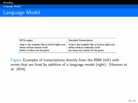
Figure: Examples of transcriptions directly from the RNN (left) witherrors that are fixed by addition of a language model (right). (Hannun etal. 2014)
50 / 59
DecodingLanguage Model
Standard approach: N-gram Model
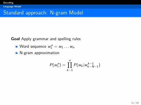
Goal Apply grammar and spelling rules
Word sequence wn1 = w1 . . .wn
N-gram approximation
P(wn1 ) =
n∏k−1
P(wk |wk−1k−N−1)
51 / 59

DecodingLanguage Model
Decoding with LM
Given a LM Hannun et. al optimizes:
arg maxw
P(w |x)P(w)α[length(w)]β
α is tunable parameter to govern weight of LMβ penalty term for long words
52 / 59

DecodingLanguage Model
Decoding with LM
Given a LM Hannun et. al optimizes:
arg maxw
P(w |x)P(w)α[length(w)]β
α is tunable parameter to govern weight of LM
β penalty term for long words
52 / 59

DecodingLanguage Model
Decoding with LM
Given a LM Hannun et. al optimizes:
arg maxw
P(w |x)P(w)α[length(w)]β
α is tunable parameter to govern weight of LMβ penalty term for long words
52 / 59

DecodingLanguage Model
Decoding with LM’s
Basic strategy Beam search to maximize
arg maxw
P(w |x)P(w)α[length(w)]β
Start with set of candidate transcript prefixes A = {}.For t = 1, . . . ,TFor each candidate in A consider
1 Add blank; dont change prefix; update probability using AM;2 Add space to prefix; update probability using LM3 Add a character to prefix; update probability using AM; Add
new candidates with updated probabilities Anew
A:=K most probable prefixes in Anew
53 / 59
DecodingLanguage Model
Neural Network Language Model
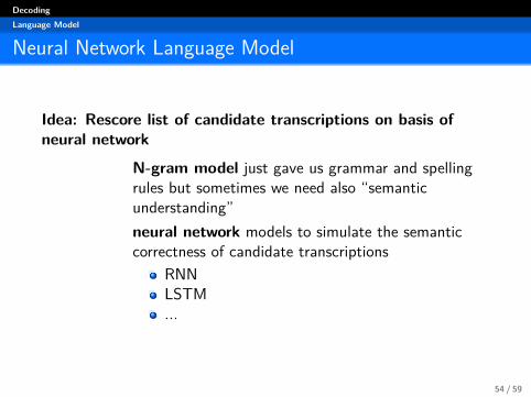
Idea: Rescore list of candidate transcriptions on basis ofneural network
N-gram model just gave us grammar and spellingrules but sometimes we need also “semanticunderstanding”neural network models to simulate the semanticcorrectness of candidate transcriptions
RNNLSTM...
54 / 59

1 Introduction
2 Architecture
3 Preprocessing
4 Decoding
5 Concluding Remarks

Concluding Remarks
End to end Speech Recognition with neon
Figure: https://www.nervanasys.com/end-end-speech-recognition-neon/55 / 59

Concluding Remarks
State of the art (IBM, March 2017)
Acoustic model score fusion of three models: one LSTMwith multiple feature inputs, a second LSTM trained withspeaker-adversarial multi-task learning and a third residual net(ResNet) with 25 convolutional layers and time-dilatedconvolutionsLanguage model word and character LSTMs andconvolutional WaveNet-style language models.
56 / 59
Concluding Remarks
Summary
Historically used approach for ASR: Dynamic Time Warpinglater statistical modelsStandard ASR Pipeline: 1.Signal Processing 2. AcousticModel 3.Language ModelSignal processing: MFCCAcoustic model two approaches: HMM and Neural Networks
GMM for HMM DistributionThree problems of HMM: Evaluation(Forward/BackwardAlgorithm), Decoding(Viterbi), Training (Baum-WelchAlgorithm)Neural networks approach: RNN, LSTM, BRNNNeural networks training: CTC
Language Model: N-gram model
57 / 59
Concluding Remarks
Future
End-to-end systems: Go deeper in the whole pipelineImage Processing: Lip reading?Train better: Batch normalization (Ioffe and Szegedy, 2015)and moreScale: More data, better data, more computational power, ...
58 / 59

Concluding Remarks
Bibliography
Connectionist Temporal Classification: Labelling UnsegmentedSequence Data with Recurrent Neural Networks (Graves etal,. 2006)Deep Speech: Scaling up end-to-end speech recognition(Hannun et al., 2014)Towards End-to-End Speech Recognition with RecurrentNeural Networks (Graves and Jaitly, 2014)Generating Sequences With Recurrent Neural Networks(Graves, 2014)Speech Recognition with Deep Recurrent Neural Networks(Graves, Mohamed and Hinton, 2013)Bidirectional Recurrent Neural Networks (Schuster andPaliwal, 1997)A Tutorial on Hidden Markov Models and SelectedApplications in Speech Recognition (Rabiner et al., 1989)
59 / 59

Concluding Remarks
Bibliography
English Conversational Telephone Speech Recognition byHumans and Machines (Saon et al.,2017)Deep Neural Networks for Acoustic Modeling in SpeechRecognition (Hinton et al.,2012)
60 / 59