energy consistent framework for continuously evolving

Available online at www.sciencedirect.com

ScienceDirect

Comput. Methods Appl. Mech. Engrg. 324 (2017) 54–73www.elsevier.com/locate/cma

Energy consistent framework for continuously evolving3D crack propagation

Łukasz Kaczmarczyk, Zahur Ullah, Chris J. Pearce∗

School of Engineering, University of Glasgow, Glasgow, G12 8QQ, UK

Received 30 September 2016; received in revised form 28 April 2017; accepted 1 June 2017Available online 15 June 2017

Highlights

• A new formulation for 3D brittle fracture in elastic solids within the context of configurational mechanics.• Continuous resolution of evolving crack path exploiting the crack front equilibrium equation.• Monolithic solution strategy for solving both material displacements (i.e. crack extension) and spatial displacements.• Problem-specific mesh smoothing with surface constraints.

Abstract

This paper presents an enhanced theoretical formulation and associated computational framework for brittle fracture in elasticsolids within the context of configurational mechanics, building on the authors’ previous paper, Kaczmarczyk et al. (2014). Thelocal form of the first law of thermodynamics provides an equilibrium condition for the crack front, expressed in terms of theconfigurational forces. Applying the principle of maximal energy dissipation, it is shown that the direction of the crack propagationis given by the direction of the configurational forces. In combination with a fracture criterion, these are utilised to determine theposition of the continuously evolving crack front. This exploitation of the crack front equilibrium condition leads to a completelynew, implicit, crack propagation formulation. A monolithic solution strategy is adopted, solving simultaneously for both thematerial displacements (i.e. crack extension) and the spatial displacements. The resulting crack path is resolved as a discretedisplacement discontinuity, where the material displacements of the nodes on the crack front change continuously, without theneed for mesh splitting or the use of enrichment techniques. In order to trace the dissipative loading path, an arc-length procedureis adopted that controls the incremental crack area growth. In order to maintain mesh quality, smoothing of the mesh is undertakenas a continuous process, together with face flipping, node merging and edge splitting where necessary. Hierarchical basis functionsof arbitrary polynomial order are adopted to increase the order of approximation without the need to change the finite element

∗ Corresponding author.E-mail addresses: [email protected] (Ł. Kaczmarczyk), [email protected] (Z. Ullah),

[email protected] (C.J. Pearce).

http://dx.doi.org/10.1016/j.cma.2017.06.0010045-7825/ c⃝ 2017 The Authors. Published by Elsevier B.V. This is an open access article under the CC BY license (http://creativecommons.org/licenses/by/4.0/).

http://crossmark.crossref.org/dialog/?doi=10.1016/j.cma.2017.06.001&domain=pdf

http://www.elsevier.com/locate/cma

http://dx.doi.org/10.1016/j.cma.2017.06.001

http://www.elsevier.com/locate/cma

mailto:[email protected]



http://dx.doi.org/10.1016/j.cma.2017.06.001

http://creativecommons.org/licenses/by/4.0/


Ł. Kaczmarczyk et al. / Comput. Methods Appl. Mech. Engrg. 324 (2017) 54–73 55

mesh. Performance of the formulation is demonstrated by means of three representative numerical simulations, demonstrating bothaccuracy and robustness.c⃝ 2017 The Authors. Published by Elsevier B.V. This is an open access article under the CC BY license (http://creativecommons.

org/licenses/by/4.0/).

Keywords: Brittle fracture; Configurational forces; Crack tracking; Mesh smoothing

1. Introduction

The serious consequences of cracks in materials and structures mean that the computational modelling of crackpropagation continues to be a critical area of research, and a major challenge. This paper presents a finite elementbased computational framework for modelling brittle crack propagation in elastic solids, based on the concept ofconfigurational mechanics. The focus of this paper is on both the mathematical formulation and the computationalframework to model and continuously resolve propagating cracks in a robust and computationally tractable manner.This paper is concerned with quasi-static problems where the influence of inertia is ignored. A sequel to this paperwill demonstrate the extension of this work to dynamic fracture.

Within the context of the finite element method, the modelling of crack propagation was traditionally undertakenin a smeared sense, whereby the problem is solved within a continuum setting, without the need for approximationof discontinuities or changing mesh connectivity. However, as strains localise, numerical difficulties arise, andregularisation is required. In contrast, discrete approaches are able to directly approximate the macroscopic crackgeometry and describe cracks in a more natural and straightforward manner in terms of displacement jumps andtractions. One of the first methods to simulate discrete crack propagation, without predefining the crack surfaces, wasthe embedded discontinuity method [1,2]. Since the enhancement in this method was local, it was computationallyefficient, but the piecewise nature of the resulting crack surface led to numerical difficulties. Partition of Unitymethods, such as the extended finite element method, represented a significant advancement to overcome this,see [3,4].

Tracking the crack path, irrespective of the methodology for resolving the resulting crack surface, is also asignificant challenge. Jager et al. [5] reviewed different discrete crack tracking algorithms for quasi-brittle fractureand undertook a systematic comparison, motivated by the challenge of undertaking crack propagation in three-dimensions. They demonstrated the difficulty in predicting and representing crack surfaces of arbitrary shape andwhich are continuous across element boundaries, and identified a global tracking algorithm by Oliver [6] as the mostalgorithmically robust, yet simple and easily implemented into existing finite element software. The criterion for crackpropagation was the classical principal stress-based Rankine criterion. However, in this paper, the need for a cracktracking methodology is obsolete, since the crack front is simply advanced by an amount and in a direction based onlyon physical laws.

The variational formulation for fracture by Francfort and Marigo [7] represented a watershed in the formulationand numerical analysis of crack evolution, recasting and generalising the engineering approach to fracture proposedby Griffith into a continuum mechanics framework as an energy minimisation problem. This removed some of theconstraints of Griffith’s original approach, for example any assumption as to the actual geometry of the crack pathor its restriction to stable crack propagation. Numerous developments have emerged from this seminal work, manyfocusing on the regularisation of the complex energy functional to make it more suitable for a numerical modelling.Most notably, the popular phase-field methods for fracture [8] have emerged where cracks are represented by a smoothdamage variable leading to a phase-field approximation of the variational formulation for brittle fracture [9,10].Although the crack surface is not represented by a discrete discontinuity, phase-field methods can be implementedin a straightforward manner using coupled multi-field finite element solvers.

This paper is focused on the concept of configurational mechanics that dates back to the original work of Eshelbyand his study of forces acting on material defects [11,12]. The concept of configurational (or material) forces isnow a well established method to evaluate defects in a material providing a unified framework for the analysis ofmaterial imperfections and has been adopted by, amongst others, Maugin [13,14]. Steinmann [15,16] developed acomputational strategy for the assessment of fractured bodies. Gurtin and Podio-Guidugli [17] derived the equationsthat govern the motion of the crack front, applied to dynamic problems in two dimensions, establishing a link between



56 Ł. Kaczmarczyk et al. / Comput. Methods Appl. Mech. Engrg. 324 (2017) 54–73

Griffith’s fracture criterion and configurational forces in two dimensions. Miehe et al. [18,19] and Kaczmarczyket al. [20] build on this work to establish a finite element methodology for crack propagation.

To formulate the crack propagation problem within the framework of configurational mechanics, two relatedkinematic descriptions are defined in the spatial and material settings. In the former, the classical conservation lawof linear momentum balance is described, where Newtonian forces are work conjugate to changes in the spatialposition, at fixed material position (i.e. no crack propagation). In the material setting, which represents a dual to thespatial setting, an equivalent conservation law is described, where configurational forces are conjugate to changesin material position but with no spatial motion. This decomposition of the behaviour is proven to be a simple butpowerful methodology for describing crack propagation. The authors’ previous paper [20] described the mathematicalformulation for crack propagation and a methodology for resolving the evolving crack path within the context ofthe finite element method, and represented an advancement of the work of Miehe et al. [18,19]. The current paperutilises the same underpinning mathematical formulation but introducing new computational strategies to continuouslyresolve the evolving crack path.

This paper brings together several key developments, establishing a new methodology for simulating 3D brittlecrack propagation, representing a significant improvement on the authors’ previous work [20]. Griffith’s fracturecriterion is expressed correctly in terms of configurational forces. An expression for equilibrium of the crack front isestablished, balancing the configurational forces on the crack front with the resistance of the material. This is exploitedso that the crack front can advance continuously, moving nodes on the crack front to the physically correct positionwithout recourse to any kind of crack tracking algorithm. There is no need for mesh splitting, or changes to meshconnectivity in order to resolve the crack front advancement, as with other approaches, e.g. [18–20]. To maintainmesh quality, a mesh smoothing strategy, with surface constraints, is presented as a continuous process as part of aproblem-tailored Arbitrary Lagrangian Eulerian formulation. This is supplemented by face flipping, node mergingand edge splitting where necessary. Post-processing of the stresses is not required to determine if the crack shouldpropagate and the crack front shape is calculated based purely on the physical equations. The spatial and materialdisplacement fields are both discretised using the same finite element mesh, although we adopt different levels ofapproximation for the two fields. The resulting discretised weak form of the two conservation equations represents aset of coupled, nonlinear, algebraic equations that is solved in a monolithic manner using a Newton–Raphson scheme.In addition, an arc-length method is adopted to trace the dissipative load path for brittle fracture propagation, usingcrack area rather than displacements as a control. Three numerical examples are presented that demonstrate the abilityof the formulation to accurately and robustly predict crack paths without bias from the original mesh.

2. Body and crack kinematics

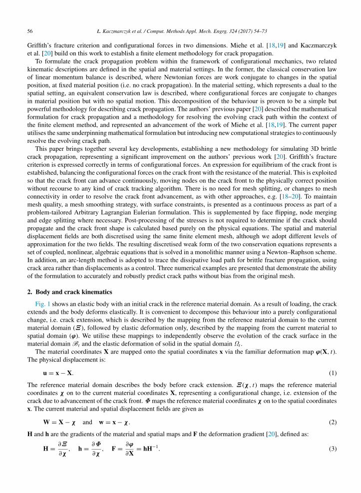
Fig. 1 shows an elastic body with an initial crack in the reference material domain. As a result of loading, the crackextends and the body deforms elastically. It is convenient to decompose this behaviour into a purely configurationalchange, i.e. crack extension, which is described by the mapping from the reference material domain to the currentmaterial domain (Ξ ), followed by elastic deformation only, described by the mapping from the current material tospatial domain (ϕ). We utilise these mappings to independently observe the evolution of the crack surface in thematerial domain Bt and the elastic deformation of solid in the spatial domain Ωt .

The material coordinates X are mapped onto the spatial coordinates x via the familiar deformation map ϕ(X, t).The physical displacement is:

u = x − X. (1)

The reference material domain describes the body before crack extension. Ξ (χ , t) maps the reference materialcoordinates χ on to the current material coordinates X, representing a configurational change, i.e. extension of thecrack due to advancement of the crack front. Φ maps the reference material coordinates χ on to the spatial coordinatesx. The current material and spatial displacement fields are given as

W = X − χ and w = x − χ . (2)

H and h are the gradients of the material and spatial maps and F the deformation gradient [20], defined as:

H =∂Ξ

∂χ, h =

∂Φ

∂χ, F =

∂ϕ

∂X= hH−1. (3)


Fig. 1. Decomposition of crack propagation in elastically deforming body.

Fig. 2. Crack construction. In 2D (left) and in more detail in 3D (right).

Given that the physical material cannot penetrate itself or reverse the movement of material coordinates, we have:

det(F) =det(h)det(H)

> 0. (4)

In addition, the time derivative of the physical displacement u and the deformation gradient F (material timederivative) are given as [20]:

u = w − FW F = ∇Xx = ∇Xu = ∇Xw − F∇XW. (5)

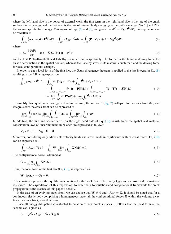
The crack surface, comprising two crack faces, is denoted as Γ and the crack front is denoted as ∂Γ , see Fig. 2.In [20], a kinematic relationship between the change in the crack surface area AΓ and the crack front velocity W wasderived that is given as:

AΓ =

∫∂Γ

A∂Γ · WdL (6)

where A∂Γ is a dimensionless kinematic state variable that defines the current orientation of the crack front. In derivingthis expression, it was recognised that any change in the crack surface area AΓ in the current material space can onlyoccur due to motion of the crack front.

3. Dissipation of energy due to creation of new crack surfaces

The first law of thermodynamics can be expressed as:∫∂Bt

u · tdS = γ AΓ +ddt

∫Bt

Ψ (F)dV (7)


where the left hand side is the power of external work, the first term on the right hand side is the rate of the cracksurface internal energy and the last term is the rate of internal body energy. γ is the surface energy [Nm−1] and Ψ isthe volume specific free energy. Making use of Eqs. (5) and (6), and given that dV = ∇X · WdV , this expression canbe rewritten as∫

∂Bt

w · t − W · FTt

dS =

∫∂Γ

γ A∂Γ · WdL +

∫Bt

P : ∇Xw + Σ : ∇XWdV (8)

where

P :=∂Ψ (F)

∂Fand Σ := Ψ (F)1 − FTP (9)

are the first Piola–Kirchhoff and Eshelby stress tensors, respectively. The former is the familiar driving force forelastic deformation in the spatial domain, whereas the Eshelby stress is its material counterpart and the driving forcefor local configurational changes.

In order to get a local form of the first law, the Gauss divergence theorem is applied to the last integral in Eq. (8)resulting in the following expression∫

∂Γ

γ A∂Γ · WdL =

∫Bt

w · ∇X · PdV +

∫Bt

W · ∇X · Σ dV

+

∫∂Bt ∪Γ+∪Γ−

w · t − PNdS +

∫∂Bt ∪Γ+∪Γ−

W · FTt + ΣNdS

− lim|C|→0

∫C

w · PNdS + lim|C|→0

∫C

W · ΣNdS.

(10)

To simplify this equation, we recognise that, in the limit, the surface C (Fig. 2) collapses to the crack front ∂Γ , andintegrals over the crack front can be expressed as

lim|C|→0

∫C

(·)dS := lim|C|→0

∫Lt

∫Ln

(·)dS =

∫∂Γ

lim|Ln|→0

∫Ln

(·)dS. (11)

In addition, the first and second terms on the right hand side of Eq. (10) vanish since the spatial and materialconservation laws of linear momentum balance are expressed as follows:

∇X · P = 0, ∇X · Σ = 0. (12)

Moreover, considering only admissible velocity fields and stress fields in equilibrium with external forces, Eq. (10)can be expressed as:∫

∂Γ

γ A∂Γ · W dL −

∫∂Γ

W · lim|Ln|→0

∫Ln

ΣN dS = 0. (13)

The configurational force is defined as

G = lim|Ln|→0

∫Ln

ΣN dL . (14)

Thus, the local form of the first law (Eq. (10)) is expressed as:

W · (γ A∂Γ − G) = 0. (15)

This equation represents the equilibrium condition for the crack front. The term γ A∂Γ can be considered the materialresistance. The exploitation of this expression, to describe a formulation and computational framework for crackpropagation, is the essence of this paper’s novelty.

In the case of an evolving crack front, we can deduce that W = 0 and γ A∂Γ = G. It should be noted that for acontinuous elastic body comprising a homogeneous material, the configurational forces G within the volume, awayfrom the crack front, should be zero.

Since all energy dissipation is restricted to creation of new crack surfaces, it follows that the local form of thesecond law is given as

D := γ W · A∂Γ = W · G ≥ 0 (16)


where D is the dissipation of energy per unit length of the crack front. This inequality restricts evolution of the crackto positive crack area growth at each point of the crack front. Although the first law defines if the crack front is inequilibrium and the second law places restrictions on the direction of crack evolution, it does not determine how A∂Γ

or W evolves. A crack growth criterion is presented in the next section.

4. Evolution of the crack front

A straightforward criterion for crack growth, equivalent to Griffith’s criterion, is proposed:

φ(G) = G · A∂Γ − gc/2 ≤ 0 (17)

where gc = 2γ is a material parameter specifying the critical threshold of energy release per unit area of the cracksurface Γ , also known as the Griffith energy. For a point on the crack front to satisfy the crack growth criterion, eitherφ < 0 and W = 0, or φ = 0, W = 0 and γ A∂Γ = G.

To determine evolution of a point on the crack front, we adopt the principle of maximum dissipation, that statesthat, for all possible configurational forces G∗ satisfying the crack growth criterion φ(G∗) = 0, the dissipation Dattains its maximum for the actual configurational force G. Therefore, we have

Dmax = (G − G∗) · W ≥ 0. (18)

This can be interpreted as an unconstrained minimisation problem, for which the Lagrangian function is:

L (G∗, κ) = −G∗· W + κφ(G∗) (19)

with κ the Lagrange multiplier. The Kuhn–Tucker conditions become∂L

∂G∗= −W + κA∂Γ = 0, κ ≥ 0, φ(G∗

∂Γ ) ≤ 0, and κφ(G∗) = 0. (20)

Thus, for a point on the evolving crack front, the crack front orientation is colinear to the configurational force(Eq. (15)), i.e. γ A∂Γ = G, and the crack extension is given as W = κA∂Γ . κ has the dimension of length andrepresents the kinematic state variable for a point on the crack front, which can be identified as:

AΓ ≡

∫∂Γ

κ dL ≥ 0. (21)

5. Spatial and material discretisation

Finite element approximation is applied for displacements in both the current material and physical space

Xh= Φ(χ )X, xh

= Φ(χ )xWh

= Φ(χ ) ˙W, wh= Φ(χ ) ˙w

(22)

where superscript h indicates approximation and (·) indicates nodal values. Three-dimensional domains are discretisedwith tetrahedral finite elements. In the spatial domain, hierarchical basis functions of arbitrary polynomial orderare applied, following the work of Ainsworth and Coyle [21]. This enables the use of elements with variable, non-uniform orders of approximation, with conformity enforced across element boundaries. In the material domain, linearapproximation is adopted, as this is sufficient for describing the crack front.

The discretised gradients of deformation are expressed as

Hh= BX(χ )X, hh

= Bx(χ )x, Fh= hh(Hh)−1

= Bx(X).x. (23)

The residual force vector in the discretised spatial domain is expressed in the classical way as:

rhs := τ fh

ext,s − fhint,s (24)

where τ is the unknown scalar load factor and fhext,s and fh

int,s are the vectors of external and internal forces, respectively,and defined as follows

fhext,s := A

TRI

∫TRI

ΦTthτ dS, fh

int,s = ATET

∫TET

(Bx)TPhdV (25)

where ATET and ATRI indicate the standard FE assembly for tetrahedral elements and triangular faces, respectively.


The discretised version of Eq. (15) establishes the material counterpart to Eq. (24), expressed as

rhm := fh

res − Gh. (26)

The nodal configurational forces, Gh, are the driving force for crack front evolution and, for the purposes ofestablishing equilibrium of the crack front, are calculated only for nodes on the crack front as

Gh:= A

TET

∫TET

(Bx)TΣ hdV . (27)

fhres is the vector of nodal material resistance forces, given as:

fhres :=

12

(Ah

Γ

)Tgc (28)

where gc is a vector of size equal to the number of nodes in the mesh, with zero for all components except thoseassociated with nodes on the crack front, where the value is gc. The matrix Ah

Γ , defined in [20], has dimensionsof length and describes the current orientation of the crack surface. Each row of matrix fh

res can be interpreted ascontaining the components of a node’s material velocity W which lead to a change of crack area. Since the cracksurface area can only change due to material displacements of the nodes of the crack front, Ah

Γ has relatively fewnon-zero rows, equal to the number of nodes on the crack front. The nodal forces of material resistance fh

res havedimensions of force and are work conjugate to the material displacement W on the crack front.

5.1. Arc-length control

The global equilibrium solution for the spatial and material displacements is obtained as a fully coupled problemusing the Newton–Raphson method, converging when the norms of the residuals are less than a given tolerance. Totrace the nonlinear response resulting from the dissipative behaviour, an arc-length technique is adopted. The systemof equations for conservation of the material and spatial momentum is supplemented by a load control equation thatimposes a constraint that controls the crack area increment during each load step. This load control equation takes theform:

rτ =

∑I

(AhΓ Xn)I −

∑I

(AhΓ Xi+1

n+1)I − ∆AΓ = 0, for I ∈ I : NI is crack front node (29)

where ∆AΓ is the prescribed increment of the crack area, i + 1 is the current iteration of load step n + 1.

6. Resolution of the propagating crack and mesh quality control

In the previous work of the authors [20], the crack front equilibrium equation (15) was established but not fullyexploited. This is addressed in this paper, establishing an implicit, continuous crack front evolution formulation.Previously, a discrete face-splitting methodology was adopted, whereby the mesh was changed to create the new cracksurfaces and crack front. The new crack front was generated by identifying element faces ahead of the current crackfront, aligning them to the direction of the configurational forces and finally splitting these faces if the crack criterionwas violated, creating a displacement discontinuity. This process was continued until equilibrium was achieved. Theapproach in the current paper is quite different, whereby the crack front advances in an implicit, continuous manner,to establish equilibrium of the crack. Mesh nodes are subsequently moved (the mesh is not split or the connectivitychanged) in order to resolve the new crack geometry.

However, in the process of moving the mesh nodes to resolve the advancing crack front, the mesh can becomedistorted, potentially creating poor quality elements, leading to numerical errors. To mitigate this effect we adoptseveral strategies:

1. Edge splitting is applied to elements behind the crack front that have become too elongated. This action willresult in the creation of new elements. It is enforced if, for a given node, there exists an adjacent edge with alength greater than 1.5 times the average edge length of all adjacent edges to the node.

2. Node merging is applied to elements ahead of the crack front that have become too contracted. This action willresult in the removal of elements. It is enforced if, for a given node, there exists an adjacent edge with a lengthless than 1/3 of the length of the longest edge adjacent to the node.


3. Face flipping is applied to elements in the vicinity of the crack front to ensure that a 3D Delaunay triangulationexists, with optimal internal angles. This is described in more detail in Section 6.1.

These procedures are utilised, if necessary, at the beginning of each load step, before the Newton–Raphsoniterations begin, when the solution is already out of equilibrium. Furthermore, in the case when new nodes are added,variables are transferred to the new mesh based upon approximation of the variables using the old mesh.

Fig. 3 demonstrates how the crack front evolves using the example of a three-point bending of a beam with aninitial corner notch. Only the projection of the FE mesh onto the crack surface is shown. Crack surface A shows anequilibrium solution, with the configurational forces identified. Crack surface B shows a subsequent configuration,where the crack front has advanced to a new equilibrium position, the nodes have moved to accommodate the crackgeometry but there has been no changes to the mesh connectivity. Crack surface C represents a further equilibriumconfiguration. The crack front has continued to advance but, to maintain mesh quality, the mesh behind the crack fronthas evolved, with new elements being created using the edge splitting procedure as required.

6.1. Face flipping

At the beginning of each load step, when the solution is out of equilibrium, a patch of elements around thecrack front is checked to ensure that it represents a 3D Delaunay triangulation. Fig. 4 demonstrates the idea in 2D.Considering the two elements on the left, edge i − k is prohibited because it lies in the interior of the circle thatintersects the nodes of element i − j − k (and element i − k − l). Flipping edge i − k will address this problem,redefining the two adjacent elements, without affecting the rest of the mesh. Thus, edge i − k is removed and replacedby edge j − l, and two new adjacent elements are formed that represent a Delaunay triangulation.

6.2. Mesh quality control

In addition to the mesh adjustments described above, a global mesh quality control procedure is also adopted in thespirit of an Arbitrary Lagrangian Eulerian (ALE) method. During the global Newton–Raphson procedure, constraintsare imposed on the shape of elements to ensure good mesh quality, but without influencing the physical response.Consequently, mesh smoothing is a continuous process in the current material domain, i.e. the domain in which thetopology evolution occurs.

The authors have proposed a volume–length measure of element quality [20,22]. This measure does not directlydetermine dihedral angles; however, it has been shown to be very effective at eliminating poor angles, thus improvingstiffness matrix conditioning and reducing interpolation errors [23,24]. As the volume–length measure is a smoothfunction of node positions, and its gradient is straightforward and computationally inexpensive to calculate, it is idealfor the problem at hand. The volume–length quality measure is defined as

q(Hh) := 6√

2V0

l3rms,0

det(Hh)dl3

rms(Hh)= q0b(Hh), b(Hh) :=

det(Hh)dl3

rms(Hh)(30)

where q0, V0 and lrms,0 are the element quality, element volume and root mean square of the element’s edge lengthsrespectively, in the reference configuration. Hh is the material deformation gradient, b is a measure of element qualitychange, relative to the reference configuration, and dlrms = lrms/ lrms,0 is the stretch of lrms,0. Element quality q0 isnormalised so that an equilateral element has quality q0 = 1 and a degenerate element (zero volume) has q0 = 0.Furthermore, b = 1 corresponds to no change and b = 0 is a change leading to a degenerate element. An elementedge length in the current material configuration is expressed as

l j (Hh) :=

√∆χT

j (Hh)THh∆χ j (31)

where ∆χ j is the distance vector of edge j in the reference configuration. Thus lrms is calculated as

lrms :=

√16

6∑j=1

l2j = lrms,0 dlrms. (32)


Fig. 3. Crack front advancement demonstrated with three-point bending of beam with initial corner notch. The lower images are snapshots of thepropagating crack front, with the arrows representing the nodal configurational forces. The projection of the mesh on the crack faces is also shown,including new elements (shown in blue). The dotted lines indicate the position of the crack front in the previous snapshots. (For interpretation ofthe references to colour in this figure legend, the reader is referred to the web version of this article.)

Fig. 4. Edge flipping in 2D to achieve Delaunay triangulation (blue dotted lines indicate circle that intersects nodes of corresponding element).

To control the quality of elements, an admissible deformation Hh is enforced such that

b(Hh) > γ for γ ∈ (0, 1). (33)

In practice, 0.1 < γ < 0.5 gives good results. This constraint on b is enforced by applying a volume–length log-barrierfunction [25] defined, for the entire mesh, as

B :=

Nel∑e=0

b2

2(1 − γ )− ln(b − γ ) (34)

where B is the barrier function for the change in element quality in the current material configuration and Nel is thenumber of elements. It can be seen that the log-barrier function rapidly increases as the quality of an element reduces,


and tends to infinity when the quality approaches the barrier γ , thus achieving the objective of penalising the worstquality elements.

In order to build a solution scheme that incorporates a stabilising force that controls element quality, a pseudo‘stress’ at the element level is defined as a counterpart to the first Piola–Kirchhoff stress as follows

Q :=∂B∂Hh = det(Hh)

l3lrms,0

l3lrms

(b

1 − γ+

1b − γ

)Q, (35)

where matrix Q is defined as follows

Q := (Hh)−T−

12

1l2lrms

6∑j=1

∆X j (∆χ j )T. (36)

It is worth noting that Q should be a zero matrix for a purely volumetric change or rigid body movement of a tetrahedralelement.

It is now possible to compute a vector of nodal pseudo ‘forces’ associated with Q as

fhq = A

TET

∫TET

BTXQ dV . (37)

6.3. Shape preserving constraints

The continuous adaption of the mesh must be constrained to preserve the surface of the domain being analysed,including the crack surface. Nodes on the surface can only be allowed to slide along the surface and not deviate fromit. In this work we start from the observation that a body’s shape can be globally characterised as a constant:

VA

= C (38)

where V is the volume of the body and A is its surface area. This can be expressed in integral form as∫B0

dV = C∫

∂B0

dS (39)

noting that13

∫B0

∇ · Xs dV = C∫

∂B0

dS (40)

where Xs are the coordinates on the surface S in the current material domain. Applying Gauss theorem we obtain∫∂B0

Xs ·N

∥N∥dS = 3C

∫∂B0

dS (41)

where N is the outer normal to the surface. The local form of this equation is given asN

∥N∥· Xs − 3C = 0 X ∈ ∂B0 (42)

where 3C is a constant given for the reference geometry. If the above constraint is satisfied, the body shape and volumeare conserved locally. An equivalent form this constraint equation is

N∥N∥

· (Xs − χ s) = 0 X ∈ ∂B0 (43)

where χ s are the original positions of the surface.To enforce the mesh quality control described in the preceding section, subject to the surface constraints described

in this section, the method of Lagrange multipliers is used, with the following functional,

L(X, λ) =

∫B0

Hh: Q dV + λ

T∫

∂B0

ΦTλ N · ΦX dξdη (Xs − χ s) (44)

where Hh and Q are functions of material positions, X and are current mesh nodal positions defined in the previoussections. ξ and η are parametrisation of surface ∂B0. Φλ and ΦX are the shape functions for Lagrange multipliers and


material coordinates respectively. Φλ are piecewise continuous functions with order of approximation equal to that ofthe material coordinates.

Calculating the stationary values of the Lagrangian results in the first(L(X, λ),X = 0

)and second

(L(X, λ),λ = 0

)Euler equations. The first is given as∫

∂B0

ΦTλ N · ΦX dξdη (Xs − χ s,0) = 0. (45)

Taking a truncated Taylor series expansion after the linear term of this nonlinear equation results in∫∂B0

ΦTλ

NΦX +

(Xs − χ s

)·

(Spin

[∂Xs

∂ξ

]· Bη − Spin

[∂Xs

∂η

]· Bξ

)dξdη δXs

=

∫∂B0

ΦTλ N · (Xs − χ s) dξdη

(46)

where the differential operators are defined as

BξδXs = Spin[∂δXs

∂ξ

]and BηδXs = Spin

[∂δXs

∂η

]. (47)

Linearising the second Euler equation leads to∫∂B0

ΦTX · NΦλdΓ · δλ

+

∫∂B0

λ (Xs − χ) ·

(Spin

[∂X∂ξ

]· Bη − Spin

[∂X∂η

]· Bξ

)dξdη δX

=

∫∂B0

λΦTX · Ndξdη.

(48)

These surface constraint equations are applied for each surface patch independently, i.e. where two surfaces meet, twoindependent sets of equations with Lagrange multipliers are applied. Moreover, these geometry preserving constraintsare not applied to the crack front, since configurational forces drive the material displacement of those nodes.

7. Linearised system of equations and implementation

A standard linearisation procedure is applied to the residuals rhm, rh

s , fhq & rτ . For the moment, the surface constraints

defined in Section 6.3 are excluded. The global equilibrium solution is obtained using the Newton–Raphson method,solving for the iterative changes in spatial displacements, current material displacements and the load factor as a fullycoupled problem. Since the material residual is non-zero only for nodes on the crack front, it is convenient, for thepurposes of presentation, to decompose the material nodal positions into those at the crack front Xf, those associatedwith surfaces Xs (crack surface and body surfaces) and the rest of the mesh Xb, i.e. X = Xf ∪ Xb ∪ Xs. The resultinglinear system of equations for iteration i and load step n + 1 is given as:⎡⎢⎢⎢⎢⎢⎢⎢⎣

∂xrhs ∂τ rh

s ∂Xfrh

s ∂Xbrh

s ∂Xsrhs

0 0 ∂Xfrτ 0 0

∂xrhm 0 ∂Xf

rhm 0 0

∂xfhq b 0 ∂Xf

fhq b ∂Xb

fhq b ∂Xs f

hq b

∂xfhq s 0 ∂Xf

fhq s ∂Xb

fhq s ∂Xs f

hq s

⎤⎥⎥⎥⎥⎥⎥⎥⎦

⎧⎪⎪⎪⎪⎪⎪⎪⎨⎪⎪⎪⎪⎪⎪⎪⎩

δxi+1

δτ i+1

δXi+1f

δXi+1b

δXi+1s

⎫⎪⎪⎪⎪⎪⎪⎪⎬⎪⎪⎪⎪⎪⎪⎪⎭= −

⎡⎢⎢⎢⎢⎢⎢⎣

rhs

rτ

rhm

fhq b

fhq s

⎤⎥⎥⎥⎥⎥⎥⎦ (49)

where Xi+1= Xi

+ δXi+1, xi+1= xi

+ δxi+1 and τ i+1= τ i

+ δτ i+1. The vectors fhq b and fh

q s are the components offhq associated with Xb and Xs respectively. This can be simplified for presentation purposes as:[

Kaa KasKsa Kss

] δqi+1

a

δXi+1s

= −

[fha

fhq s

](50)

where qa is the vector of all unknowns excluding the nodal coordinates of the surfaces, Xs, fha the corresponding terms

on the right hand side of Eq. (49).


In order to preserve the surfaces of the body during the analysis, it is necessary to impose the constraints describedin Section 6.3 on the coordinates of the surface nodes, Xs. Thus, the above system of equations is augmented asfollows:⎡⎣Kaa Kas 0

Ksa Kss + B CT

0 C + A 0

⎤⎦⎧⎪⎪⎨⎪⎪⎩

δqi+1a

δXi+1s

δλi+1

⎫⎪⎪⎬⎪⎪⎭ = −

⎡⎢⎢⎣fha

fhq s + CTλ

C(Xs − χ s)

⎤⎥⎥⎦ (51)

where

C = ATRI

∫TRI

ΦTλ N · ΦXdξdη, (52)

B = ATRI

∫TRI

λΦTX

(Spin

[∂X∂ξ

]· Bη − Spin

[∂X∂η

]· Bξ

)dξdη (53)

and

A = ATRI

∫TRI

ΦTλ

(Xs − χ s

)·

(Spin

[∂X∂ξ

]· Bη − Spin

[∂X∂η

]· Bξ

)dξdη. (54)

When solving this nonlinear system of equations, convergence is quadratic and typically requires 3–4 iterationsper load step to achieve convergence. We adopt a Total ALE approach; at the beginning of each new load step thecurrent material mesh becomes the new reference mesh. Discretisation is undertaken using 3D tetrahedral elementswith hierarchical basis functions of arbitrary polynomial order [21] in the spatial domain. A linear approximation isadopted in the material domain.

The solution strategy presented in this paper is implemented for parallel shared memory computers, utilising open-source libraries. MOAB, a mesh-oriented database [26], is used to store mesh data, including input and output opera-tions and information about mesh topology. PETSc (Portable, Extensible Toolkit for Scientific Computation [27]) isused for parallel matrix and vector operations, the solution of linear system of equations and other algebraic operations.MOAB and PETSc are integrated in MoFEM [28], which is an open source code for finite element analysis, developedand maintained by our group.

8. Numerical examples

Three numerical examples of crack propagation in brittle materials are presented. Two examples consider thefracture of unirradiated nuclear graphite. The third example considers the fracture of PMMA.

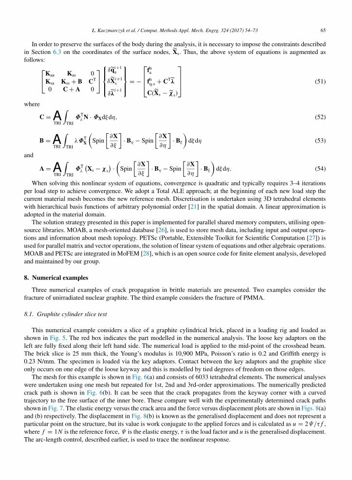
8.1. Graphite cylinder slice test

This numerical example considers a slice of a graphite cylindrical brick, placed in a loading rig and loaded asshown in Fig. 5. The red box indicates the part modelled in the numerical analysis. The loose key adaptors on theleft are fully fixed along their left hand side. The numerical load is applied to the mid-point of the crosshead beam.The brick slice is 25 mm thick, the Young’s modulus is 10,900 MPa, Poisson’s ratio is 0.2 and Griffith energy is0.23 N/mm. The specimen is loaded via the key adaptors. Contact between the key adaptors and the graphite sliceonly occurs on one edge of the loose keyway and this is modelled by tied degrees of freedom on those edges.

The mesh for this example is shown in Fig. 6(a) and consists of 6033 tetrahedral elements. The numerical analyseswere undertaken using one mesh but repeated for 1st, 2nd and 3rd-order approximations. The numerically predictedcrack path is shown in Fig. 6(b). It can be seen that the crack propagates from the keyway corner with a curvedtrajectory to the free surface of the inner bore. These compare well with the experimentally determined crack pathsshown in Fig. 7. The elastic energy versus the crack area and the force versus displacement plots are shown in Figs. 8(a)and (b) respectively. The displacement in Fig. 8(b) is known as the generalised displacement and does not represent aparticular point on the structure, but its value is work conjugate to the applied forces and is calculated as u = 2Ψ/τ f ,where f = 1N is the reference force, Ψ is the elastic energy, τ is the load factor and u is the generalised displacement.The arc-length control, described earlier, is used to trace the nonlinear response.


Fig. 5. Experimental loading frame for graphite cylinder slice test. All dimensions in mm.

Fig. 6. Geometry and crack path for graphite cylinder slice test.

Snapshots of the brick slice at three points S1, S2 and S3, shown in Fig. 8 are shown in Fig. 9(a), (b) and (c)respectively. It should be noted that Fig. 8 demonstrates that, as compared to the fluctuating results for 1st-orderanalysis, the results for 2nd and 3rd-order analyses are very smooth. The fluctuation in the results for the 1st orderanalysis is due to shear locking.

8.2. Mixed mode I–III loading in three-point bending test

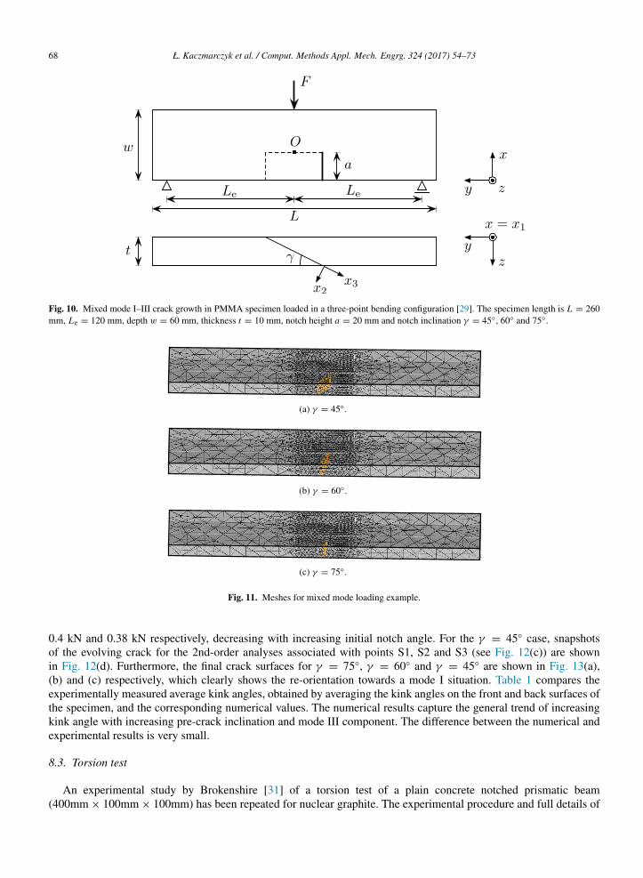
The second example assesses the ability of the proposed approach to simulate the mixed mode I–III experimentsof [29] on PMMA pre-notched beams loaded in a three-point-bending configuration. This problem was also simulatedby Pandolfi and Ortiz [30] (although they did not model the entire specimen, instead restricting calculations to thecentral section of the specimen, applying equivalent static boundary conditions representative of three-point bending).The specimens are 260 mm long, 60 mm deep, and 10 mm thick, pre-cracked at 45, 60, and 75 to the front face,


Fig. 7. Experimentally determined crack paths for graphite cylinder slice test.

(a) Elastic energy versus crack area. (b) Force versus displacement.

Fig. 8. Energy versus crack area and load versus displacement plots for graphite cylinder slice test.

(a) Snapshot at S1. (b) Snapshot at S2. (c) Snapshot at S3.

Fig. 9. Snapshots for points S1, S2 and S3 shown in Fig. 8 for graphite cylinder slice test.

Fig. 10. Consistent with [29], Young’s modulus E = 2800 MPa, Poisson’s ratio ν = 0.38, and Griffith energy0.352 N/mm are used. The inclination of the notch results in an initial mixed mode I–III loading of the crack front.The experiments demonstrated that for homogeneous and linear-elastic isotropic materials the growing crack, loadedin mixed I–III modes, reorientates towards a pure mode I situation. The meshes are shown in Fig. 11 and consist of8696, 7824 and 8705 tetrahedral elements for 45, 60, and 75 initial notch angles respectively.

All three cases are solved for 1st, 2nd and 3rd-order of approximation. Elastic energy versus crack area plots areshown in Fig. 12(a). Consistent with the previous example, the response for all three cases fluctuates for the 1st-orderanalysis but is smooth for the 2nd and 3rd-order analyses. Fig. 12(b) compares the load–displacement response forγ = 60, for different orders of approximation. Fig. 12(c) compares the load–displacement response for 2nd-orderapproximations, for all three initial notch angles. The ultimate load for γ = 45, γ = 60 and γ = 75 is 0.46 kN,


Fig. 10. Mixed mode I–III crack growth in PMMA specimen loaded in a three-point bending configuration [29]. The specimen length is L = 260mm, Le = 120 mm, depth w = 60 mm, thickness t = 10 mm, notch height a = 20 mm and notch inclination γ = 45, 60 and 75.

(a) γ = 45.

(b) γ = 60.

(c) γ = 75.

Fig. 11. Meshes for mixed mode loading example.

0.4 kN and 0.38 kN respectively, decreasing with increasing initial notch angle. For the γ = 45 case, snapshotsof the evolving crack for the 2nd-order analyses associated with points S1, S2 and S3 (see Fig. 12(c)) are shownin Fig. 12(d). Furthermore, the final crack surfaces for γ = 75, γ = 60 and γ = 45 are shown in Fig. 13(a),(b) and (c) respectively, which clearly shows the re-orientation towards a mode I situation. Table 1 compares theexperimentally measured average kink angles, obtained by averaging the kink angles on the front and back surfaces ofthe specimen, and the corresponding numerical values. The numerical results capture the general trend of increasingkink angle with increasing pre-crack inclination and mode III component. The difference between the numerical andexperimental results is very small.

8.3. Torsion test

An experimental study by Brokenshire [31] of a torsion test of a plain concrete notched prismatic beam(400mm × 100mm × 100mm) has been repeated for nuclear graphite. The experimental procedure and full details of


(a) (b) For γ = 60.

(c) For 2nd order analyses. (d) For γ = 45.

Fig. 12. Elastic energy versus crack area and force versus displacement plots for 1st-, 2nd- and 3rd-order of approximation and various initial crackinclinations for mixed mode loading example.

(a) λ = 75.

(b) λ = 60.

(c) λ = 45.

Fig. 13. Final crack surfaces for various pre-crack inclinations for mixed mode loading example.


Table 1Comparison of experimental [29] and numerical initial kink angle fordifferent notch inclinations.

γ Experiment [29] Numerical Error %

45 61.9 56.02 9.4960 38.4 37.46 2.4575 21.1 20.87 1.09

(a) Geometry with dimensions. (b) Mesh.

Fig. 14. Geometry and mesh for torsion test.

(a) Elastic energy versus crack area. (b) Force versus displacement.

Fig. 15. (a) Elastic energy versus crack area and (b) load versus displacement plots for torsion test.

the boundary conditions and dimensions for the original study are described in Jefferson et al. [32] and illustrated inFig. 14(a). The notch is placed at an oblique angle across the beam and extends to half the depth. The beam is placedin a steel loading frame, supported at three corners and loaded at the fourth corner. The material properties used forthis example are the same as those used in the graphite cylinder slice test example.

The beam and steel frame are discretised using tetrahedral elements and are shown in Fig. 14(b). The mesh consistsof 11890 elements and the problem is solved with 1st, 2nd and 3rd-order approximation. Fig. 15(a) and (b) shows theelastic energy-crack area and load–displacement response for the three numerical tests respectively. Good numericalconvergence is observed with increasing order of approximation and the arc-length control method is able to trackthe dissipative loading path. The ultimate load for 1st, 2nd and 3rd-order approximation is 0.326 kN, 0.294 kNand 0.291 kN respectively. The snapshots of evolving crack at points S1, S2 and S3 (see Fig. 15(b)), are shown inFig. 16(a), (b) and (c) respectively. The front and top views of the simulated crack surface are also shown in Fig. 17(a)and (b) respectively, which clearly shows the complicated crack path. It is worth noting that the same problem wasdiscussed in our previous paper [20] but the material was concrete rather than graphite. In this previous case the crack


(a) Snapshot at S1. (b) Snapshot at S2. (c) Snapshot at S3.

Fig. 16. Snapshots for points S1, S2 and S3 shown in Fig. 15 for torsion test.

(a) Front view.

(b) Top view.

Fig. 17. The simulated crack surface viewed from front and top for torsion test.

path showed excellent agreement with experiments but over predicted the experimental ultimate load by approximately2.5 times. This was a consequence of assuming linear elastic fracture mechanics for a problem where the size of thefracture process zone is significant compared to the size of the problem. This is not an issue in the current situationbecause graphite’s microstructure is significantly smaller than for concrete and the assumption of linear elastic fracturemechanics is valid.


9. Conclusions

A novel formulation for brittle fracture in elastic solids within the context of configurational mechanics has beenpresented that incorporate several advancements on the authors’ previous work. The local form of the first law ofthermodynamics provides a condition for equilibrium of the crack front and the direction of crack propagation isgiven by the configurational forces on the crack front, maximising the local dissipation. These are exploited such thatthe advancing crack front is continuously resolved by moving the nodes of the finite element mesh, without the needfor face splitting or the use of enrichment techniques.

A monolithic solution strategy has been described that simultaneously solves for both the material displacements(i.e. crack extension) and the spatial displacements. In order to trace the dissipative loading path, an arc-lengthprocedure has been developed that controls the incremental crack area growth. In order to maintain mesh quality,smoothing of the mesh is undertaken as a continuous process, together with face flipping, node merging and edgesplitting where necessary. Hierarchical basis functions of arbitrary polynomial order are adopted to increase the orderof approximation without the need to change the finite element mesh.

Three numerical examples have been presented to demonstrate both the accuracy and robustness of the formulation.Convergence studies have been undertaken in all cases. All three problems demonstrate the ability to simulateexperimental crack paths.

Acknowledgements

This work was supported by EDF Energy Nuclear Generation Ltd (grant no. 4840360333) and The Royal Academyof Engineering (grant no. RCSRF1516\2\18). The views expressed in this paper are those of the authors and notnecessarily those of EDF Energy Nuclear Generation Ltd. Analyses were undertaken using the EPSRC fundedARCHIE-WeSt High Performance Computer (www.archie-west.ac.uk, EPSRC grant no. EP/K000586/1).

References

[1] J. Oliver, Modelling strong discontinuities in solid mechanics via strain softening constitutive equations. 1. fundamentals, Internat. J. Numer.Methods Engrg. 39(21) (1996) 3575–3600.

[2] J. Oliver, Modelling strong discontinuities in solid mechanics via strain softening constitutive equations. 2: Numerical simulation, Internat. J.Numer. Methods Engrg. 39(21) (1996) 3601–3623.

[3] J. Dolbow, N. Moës, T. Belytschko, Discontinuous enrichment in finite elements with a partition of unity method, Finite Elem. Anal. Des.36(3–4) (2000) 235–260.

[4] J. Dolbow, N. Moës, T. Belytschko, A finite element method for crack growth without remeshing, Internat. J. Numer. Methods Engrg. 46(1)(1999) 131–150.

[5] P. Jäger, P. Steinmann, E. Kuhl, Modeling three-dimensional crack propagation - a comparison of crack path tracking strategies, Internat. J.Numer. Methods Engrg. 76(9) (2008) 1328–1352.

[6] J. Oliver, A. Huespe, E. Samaniego, E. Chaves, Continuum approach to the numerical simulation of material failure in concrete, Int. J. Numer.Anal. Methods Geomech. 28(7–8) (2004) 609–632.

[7] G. Francfort, J. Marigo, Revisiting brittle fracture as an energy minimisation problem, J. Mech. Phys. Solids 46(8) (1998) 1319–1342.[8] B. Bourdin, G. Francfort, J. Marigo, Numerical experiments in revisited brittle fracture, J. Mech. Phys. Solids 48(4) (2000) 797–826.[9] C. Miehe, F. Welschinger, M. Hofacker, Thermodynamically consistent phase-field models of fracture: Variational principles and multi-field

FE implementations, Internat. J. Numer. Methods Engrg. 83(10) (2010) 1273–1311.[10] C. Kuhn, R. Müller, A continuum phase field model for fracture, Eng. Fract. Mech. 77(18) (2010) 3625–3634.[11] J. Eshelby, The force on an elastic singularity, Phil. Trans. R. Soc. A 224(877) (1951) 87–112.[12] J. Eshelby, Energy relations and the energy-momentum tensor in continuum mechanics, in: M.F. Kanninen, et al. (Eds.), Inelastic Behavior

of Solids (1970) 77–115.[13] G.A. Maugin, Material Inhomogeneities in Elasticity, Vol. 3, CRC Press, 1993.[14] G.A. Maugin, Configurational Forces: Thermomechanics, Physics, Mathematics, and Numerics, CRC Press, 2016.[15] P. Steinmann, Application of material forces to hyperelastic fracture mechanics. I. Continuum mechanical setting, Int. J. Solids Struct.

37(48–50) (2000) 7371–7391.[16] P. Steinmann, D. Ackermann, F. Barth, Application of material forces to hyperelastic fracture mechanics. II. Computational setting, Int. J.

Solids Struct. 38(32–33) (2001) 5509–5526.[17] M. Gurtin, P. Podio-Guidugli, Configurational forces and the basic laws for crack propagation, J. Mech. Phys. Solids 44(6) (1996) 905–927.[18] C. Miehe, E. Gürses, M. Birkle, A computational framework of configurational-force-driven brittle fracture propagation based on incremental

energy minimization, Int. J. Fract. 145(4) (2007) 245–259.[19] E. Gürses, C. Miehe, A computational framework of three-dimensional configurational-force-driven brittle crack propagation, Comput.

Methods Appl. Mech. Engrg. 198(15–16) (2009) 1413–1428.

http://www.archie-west.ac.uk





















http://refhub.elsevier.com/S0045-7825(16)31265-8/sb1












































[20] Ł. Kaczmarczyk, M.M. Nezhad, C. Pearce, Three-dimensional brittle fracture: configurational-force-driven crack propagation, Int. J. Numer.Methods Eng. 97(7) (2014) 531–550.

[21] M. Ainsworth, J. Coyle, Hierarchic finite element bases on unstructured tetrahedral meshes, Internat. J. Numer. Methods Engrg. 58(14) (2003)2103–2130.

[22] A. Kelly, Ł. Kaczmarczyk, C. Pearce, Mesh improvement methodology for 3D volumes with non-planar surfaces, Eng. Comput. 30(2) (2014)201–210.

[23] J. Shewchuk, What is a Good Linear Finite Element? - Interpolation, Conditioning, Anisotropy, and Quality Measures, Tech. Rep., In Proc.of the 11th International Meshing Roundtable, 2002.

[24] B. Klingner, Tetrahedral Mesh Improvement, (Ph.D. thesis), University of California at Berkeley, 2008.[25] M. Scherer, R. Denzer, P. Steinmann, On a solution strategy for energy-based mesh optimization in finite hyperelastostatics, Comput. Methods

Appl. Mech. Engrg. 197(6–8) (2008) 609–622.[26] T. Tautges, R. Meyers, K. Merkley, C. Stimpson, C. Ernst, MOAB: A Mesh-Oriented Database, Sandia Report, Sandia National Laboratories,

2004.[27] S. Balay, J. Brown, K. Buschelman, W. Gropp, D. Kaushik, M. Knepley, L. McInnes, B. Smith, H. Zhang, Portable, Extensible Toolkit for

Scientific Computation, 2012 http://www.mcs.anl.gov/petsc.[28] Ł. Kaczmarczyk, Z. Ullah, K. Lewandowski, X.-Y. Zhou, C. Pearce, MoFEM-v0.5.42 [Computer Software], University of Glasgow, 2017,

https://doi.org/10.5281/zenodo.438712.[29] V. Lazarus, F.-G. Buchholz, M. Fulland, J. Wiebesiek, Comparison of predictions by mode II or mode III criteria on crack front twisting in

three or four point bending experiments, Int. J. Fract. 153(2) (2008) 141–151.[30] A. Pandolfi, M. Ortiz, An eigenerosion approach to brittle fracture, Int. J. Numer. Methods Eng. 92(8) (2012) 694–714.[31] D. Brokenshire, A Study of Torsion Fracture Tests, Cardiff University, UK, 1996.[32] A. Jefferson, B. Barr, T. Bennett, S. Hee, Three dimensional finite element simulation of fracture test using craft concrete model, Comput.

Conc. 1(3) (2004) 261–284.




















http://www.mcs.anl.gov/petsc




























https://doi.org/10.5281/zenodo.438712













































energy consistent framework for continuously evolving

Documents