energy and greenhouse gas emissions for the seq water strategy · energy and greenhouse gas...
TRANSCRIPT

Energy and Greenhouse Gas Emissions for the SEQ Water Strategy
Hall, M1, West, J1, Lane, J2, de Haas, D3, and Sherman, B1
September 2009
Urban Water Security Research AllianceTechnical Report No. 14

Urban Water Security Research Alliance Technical Report ISSN 1836-5566 (Online) Urban Water Security Research Alliance Technical Report ISSN 1836-5558 (Print) The Urban Water Security Research Alliance (UWSRA) is a $50 million partnership over five years between the Queensland Government, CSIRO’s Water for a Healthy Country Flagship, Griffith University and The University of Queensland. The Alliance has been formed to address South-East Queensland's emerging urban water issues with a focus on water security and recycling. The program will bring new research capacity to South-East Queensland tailored to tackling existing and anticipated future issues to inform the implementation of the Water Strategy. For more information about the:
UWSRA - visit http://www.urbanwateralliance.org.au/ Queensland Government - visit http://www.qld.gov.au/ Water for a Healthy Country Flagship - visit www.csiro.au/org/HealthyCountry.html The University of Queensland - visit http://www.uq.edu.au/ Griffith University - visit http://www.griffith.edu.au/
Enquiries should be addressed to: The Urban Water Security Research Alliance PO Box 15087 CITY EAST QLD 4002 Ph: 07-3247 3005; Fax: 07-3405 3556 Email: [email protected]
Authors: 1 – CSIRO; 2 – Queensland Department of Environment and Resource Management; 3 – GHD Hall, M., West, J., Lane, J., de Haas, D. and Sherman, B., (2009). Energy and Greenhouse Gas Emissions for the SEQ Water Strategy. Urban Water Security Research Alliance Technical Report No. 14.
Copyright
© 2009 CSIRO. To the extent permitted by law, all rights are reserved and no part of this publication covered by copyright may be reproduced or copied in any form or by any means except with the written permission of CSIRO.
Disclaimer
The partners in the UWSRA advise that the information contained in this publication comprises general statements based on scientific research and does not warrant or represent the accuracy, currency and completeness of any information or material in this publication. The reader is advised and needs to be aware that such information may be incomplete or unable to be used in any specific situation. No action shall be made in reliance on that information without seeking prior expert professional, scientific and technical advice. To the extent permitted by law, UWSRA (including its Partner’s employees and consultants) excludes all liability to any person for any consequences, including but not limited to all losses, damages, costs, expenses and any other compensation, arising directly or indirectly from using this publication (in part or in whole) and any information or material contained in it. Cover Photograph:
© 2009 CSIRO

Energy and Greenhouse Gas Emissions for the SEQ Water Strategy Page i
ACKNOWLEDGEMENTS
This research was undertaken as part of the South East Queensland Urban Water Security Research Alliance, a scientific collaboration between the Queensland Government, CSIRO, The University of Queensland and Griffith University. Particular thanks go to Steve Kenway for data collection and initial leadership of the project. Many thanks also to Alan Grinham and Seqwater for use of reservoir methane data, the Project Reference Panel for focusing the project direction as well as Shiroma Maheepala, Don Begbie and Sharon Wakem for their support of the project.

Energy and Greenhouse Gas Emissions for the SEQ Water Strategy Page ii
FOREWORD
Water is fundamental to our quality of life, to economic growth and to the environment. With its booming economy and growing population, Australia's South-East Queensland (SEQ) region faces increasing pressure on its water resources. These pressures are compounded by the impact of climate variability and accelerating climate change.
The Urban Water Security Research Alliance, through targeted, multidisciplinary research initiatives, has been formed to address the region’s emerging urban water issues.
As the largest regionally focused urban water research program in Australia, the Alliance is focused on water security and recycling, but will align research where appropriate with other water research programs such as those of other SEQ water agencies, CSIRO’s Water for a Healthy Country National Research Flagship, Water Quality Research Australia, e-Water CRC and the Water Services Association of Australia (WSAA).
The Alliance is a partnership between the Queensland Government, CSIRO’s Water for a Healthy Country National Research Flagship, The University of Queensland and Griffith University. It brings new research capacity to SEQ, tailored to tackling existing and anticipated future risks, assumptions and uncertainties facing water supply strategy. It is a $50 million partnership over five years.
Alliance research is examining fundamental issues necessary to deliver the region's water needs, including:
ensuring the reliability and safety of recycled water systems.
advising on infrastructure and technology for the recycling of wastewater and stormwater.
building scientific knowledge into the management of health and safety risks in the water supply system.
increasing community confidence in the future of water supply.
This report is part of a series summarising the output from the Urban Water Security Research Alliance. All reports and additional information about the Alliance can be found at http://www.urbanwateralliance.org.au/about.html. Chris Davis Chair, Urban Water Security Research Alliance
Energy and Greenhouse Gas Emissions for the SEQ Water Strategy Page iii
CONTENTS
Acknowledgements ................................................................................................................. i
Foreword ................................................................................................................................. ii
Contents ................................................................................................................................. iii
Executive Summary................................................................................................................ 1
1. Introduction.................................................................................................................... 3
2. Aim.................................................................................................................................. 3
3. Methodology .................................................................................................................. 4
4. System Boundary and Sources of Greenhouse Gas Emissions .............................. 5 4.1. Uncertainty Estimates......................................................................................................... 6
4.2. Energy Use for Centralised Water Systems ....................................................................... 8 4.2.1. Existing WTPs .................................................................................................................. 8 4.2.2. Water Sources to 2056................................................................................................... 10
4.3. Energy Use for Rainwater Tanks...................................................................................... 12
4.4. Diffuse Emissions from Urban Water Reservoirs ............................................................. 13
4.5. Energy Use for Centralised Wastewater Systems............................................................ 20
4.6. Energy Use for On-Site Wastewater Systems.................................................................. 24
4.7. Diffuse Emissions from Centralised Wastewater Systems............................................... 25
4.8. Diffuse Emission from On-Site Wastewater Systems....................................................... 26
5. Energy and Greenhouse Gas Emissions for the Draft SEQ Water Strategy.......... 27 5.1. Energy............................................................................................................................... 27
5.1.1. Calibration to the Draft SEQ Water Strategy .................................................................. 27 5.1.2. Energy for Water and Wastewater.................................................................................. 28
5.2. Greenhouse Gas Emissions ............................................................................................. 31 5.2.1. Greenhouse Gas Emissions for Water and Wastewater ................................................ 31 5.2.2. Breakdown of Greenhouse Gas Emissions for Water Supply ........................................ 31 5.2.3. Breakdown of Greenhouse Gas Emissions for Wastewater ........................................... 32
5.3. Sensitivity of Energy and Greenhouse Gas Emissions to Reduced Demand.................. 33
6. Conclusions .................................................................................................................35
7. References ...................................................................................................................36
Appendix 1. Data Derivation for GIS Layer of WTPs .........................................................38
Appendix 2. Details of Data Sources for Energy Intensity of Mains Water Supply........39
Appendix 3. Breakdown of Pumping and Treatment Energy for Water Supply .............42
Appendix 4. Derivation of Data in GIS Layer of WTPs, and Attribution of Sewage Treatment and Pumping Energy at Sub-Regional Scale .........................................44
Appendix 5. Notes on STP Scale, Technology, and Observed Energy Intensities ........45
Appendix 6. Technical Background for Greenhouse Gas Emissions from Reservoirs....................................................................................................................46
Appendix 7. Centralised Wastewater Diffuse Greenhouse Gas Emissions....................60
Appendix 8. On-site Wastewater Diffuse GHG Emissions................................................64

Energy and Greenhouse Gas Emissions for the SEQ Water Strategy Page iv
LIST OF FIGURES
Figure 1: Simplified data collection process (ISO, 2006b). ............................................................................... 4 Figure 2: Summary of sources of greenhouse gas emissions considered for operation of water and
wastewater services. ......................................................................................................................... 5 Figure 3: Water treatment plants and mains distribution pipe network for SEQ. .............................................. 9 Figure 4: Above-ground rainwater tank installation with mains water top-up and rainwater supplied to
appliances in the household (MPMSAA, 2008). .............................................................................. 13 Figure 5: Conceptual model of CO2 (top) and CH4 (bottom) cycles in reservoirs (figure from Sherman
et al. 2001). ..................................................................................................................................... 15 Figure 6: Methane emissions from Wivenhoe Dam. Figure courtesy A. Grinham, University of
Queensland. .................................................................................................................................... 16 Figure 7: Reservoir methane emissions as a function of catchment area. ..................................................... 17 Figure 8: Estimated methane emissions from reservoirs in South-East Queensland. Green bars
denote medium emissions estimated using the emission level (80 mg CH4 m-2 d-1) from Borumba dam. Orange bars denote emissions computed using catchment area-specific emission regression from Figure 7. ................................................................................................. 18
Figure 9: Total estimated annual methane flux (expressed as CO2-e) from SEQ reservoirs for low, medium and high areal emission rates and using the catchment area-specific regression to determine the emission rate. ........................................................................................................... 18
Figure 10: Change in reservoir GHG emissions over time. Data courtesy L. Gagnon, pers. comm. 2001. ...... 20 Figure 11: Wastewater treatment plants in SEQ with rated capacity greater than 500 EP. .............................. 21 Figure 12: Gross plant power (flow-specific) including lift pumps and UV vs ADWF. ....................................... 23 Figure 13: Corrected plant power (flow-specific), excluding lift pumps, vs. current ADWF............................... 23 Figure 14: Corrected plant power (flow-specific), excluding lift pumps. ............................................................ 24 Figure 15: Comparison of energy for grid water to the draft SEQ Water Strategy (figure 6.13 from QWC
2008). .............................................................................................................................................. 28 Figure 16: Energy for water and wastewater. Uncertainties are shown with dashed lines and using the
same colour as the mode. ............................................................................................................... 28 Figure 17: Energy for centralised and decentralised water. Uncertainties are shown with dashed lines
and using the same colour as the mode.......................................................................................... 29 Figure 18: Comparison of energy use for centralised water pumping and treatment. Uncertainties are
shown with dashed lines and using the same colour as the mode. ................................................. 30 Figure 19: Energy for centralised and decentralised wastewater. Uncertainties are shown with dashed
lines and using the same colour as the mode. ................................................................................ 30 Figure 20: Greenhouse gas emissions for water and wastewater. Uncertainties are shown with dashed
lines and using the same colour as the mode. ................................................................................ 31 Figure 21: Breakdown of water supply greenhouse gas emissions. Uncertainties are shown with
dashed lines and using the same colour as the mode..................................................................... 32 Figure 22: Breakdown of wastewater greenhouse gas emissions. Uncertainties are shown with dashed
lines and using the same colour as the mode. ................................................................................ 33 Figure 23: Sensitivity of centralised water energy use to changes in demand. Uncertainties are shown
with dashed lines and using the same colour as the mode. ............................................................ 34
LIST OF TABLES
Table 1: Data accuracy rating and corresponding intervals used in the GHG Protocol uncertainty tool.......... 6 Table 2: Summary of uncertainty estimates. ................................................................................................... 7 Table 3: Energy intensities for different processes at four major WTPs in SEQ............................................ 10 Table 4: Energy intensity of water supply tasks by source. ........................................................................... 11 Table 5: Measured methane emissions from Australian reservoirs. .............................................................. 16 Table 6: Methane emission estimates for SEQ reservoirs. ALL CAPS denotes reservoir data sourced
from ICOLD. All other data sourced from utility web sites. .............................................................. 19 Table 7: Sewage treatment and pumping energy intensities for reticulated urban demand. ......................... 22 Table 8: Decentralised wastewater system energy intensities. ..................................................................... 24

Energy and Greenhouse Gas Emissions for the SEQ Water Strategy Page 1
EXECUTIVE SUMMARY
The sustainability challenge for water and wastewater services in South-East Queensland (SEQ) is framed by water shortages, a rapidly growing population, stressed aquatic ecosystems and uncertain climate change. In turn, measures to provide water and wastewater services have implications for energy and greenhouse gas emissions.
The study aimed to inform long-term planning strategies, such as the SEQ Water Strategy, of the largest contributors to and long-term trends for operational energy use and greenhouse gas emissions for urban water and wastewater services. In particular, the relative contribution to greenhouse gas emissions was sought for:
centralised water and wastewater services; decentralised (on-site) water and wastewater systems; and diffuse emissions from wastewater treatment and handling and urban water reservoirs. Energy for pumping is much greater than treatment energy for centralised water services in SEQ. Pumping currently accounts for approximately 80% of energy use for centralised water services. However, this relationship will change if desalination plants (with high treatment energy use) are operated above minimum levels.
Energy savings from successful water demand management are constrained by the need to operate desalination plants due to plant design and SEQ System Operating Plan requirements. As a result, a 25% reduction in water demand only reduces water system energy use by about 10% for the two decades following demand reduction. Greater energy savings are not achieved because desalinated water is supplied even when low-energy water supplies are available.
Greenhouse gas emissions from energy use for water and wastewater services in SEQ will rise faster than growth in population – more than doubling over the next 50 years. New sources of water supply such as desalination, recycled water and rainwater tanks currently have greater energy intensity than traditional sources.
Diffuse greenhouse gas emissions are potentially much greater than emissions from energy use for the sector – although the data currently has a very high level of uncertainty. The main sources of diffuse emissions include reservoirs as well as wastewater treatment and handling.
The 800,000 new rainwater tanks that are planned to be installed in SEQ over the next 50 years may use as much energy as the current centralised water supply if installed and operated at the upper ranges of current energy use. There is a large range in efficiency and appropriate guidance for tank set up could significantly reduce this impact.
A handful of large water and wastewater plants account for the bulk of treatment capacity. For wastewater treatment plants there was a weak correlation between plant size and energy efficiency.
Assuming the scenario of the SEQ Water Strategy (and prioritising low-energy water supplies subject to operating constraints), Figures 1ES and 2ES provide an overview of greenhouse gas emissions for water and wastewater services over the next 50 years.
Future directions for research and potential mitigation should focus on sources of energy use and greenhouse gas emissions that make a large contribution to system results and have high levels of uncertainty. These include diffuse greenhouse gas emissions from reservoirs and wastewater systems and energy use from rainwater tanks. In addition, the scope of the research should be expanded beyond energy use and greenhouse gas emissions to other key environmental issues for the water sector such as aquatic ecosystem impacts. Consideration of economic and social considerations would also allow an evaluation of sustainability and comparison of options.
In this context, the information presented in this report expands energy use and greenhouse gas emissions considerations for the SEQ urban water sector. It provides valuable information to help understand the sustainability challenge of water and wastewater services in SEQ over the coming decades.

Energy and Greenhouse Gas Emissions for the SEQ Water Strategy Page 2
0
200000
400000
600000
800000
1000000
1200000
1400000
1600000
1800000
2000000
2008
2011
2014
2017
2020
2023
2026
2029
2032
2035
2038
2041
2044
2047
2050
2053
2056
YEAR
GR
EE
NH
OU
SE
GA
S E
MIS
SIO
NS
(to
nn
e C
O2-
e)
RAINWATER TANKS RESERVOIR METHANE CENTRALISED WATER
Figure 1ES: Greenhouse gas emissions for water services. Uncertainties were estimated following IPCC Good Practice Guidelines (IPCC, 2000) and are shown by dashed lines colour-coded to modes.
0
100000
200000
300000
400000
500000
600000
2008
2010
2012
2014
2016
2018
2020
2022
2024
2026
2028
2030
2032
2034
2036
2038
2040
2042
2044
2046
2048
2050
2052
2054
2056
YEAR
GR
EE
NH
OU
SE
GA
S E
MIS
SIO
NS
(to
nn
e C
O2-
e)
ON-SITE WASTEWATER ENERGYON-SITE WASTERWATER METHANECENTRALISED WASTEWATER ENERGYCENTRALISED WASTEWATER DIFFUSE EMISSIONS
Figure 2ES: Greenhouse gas emissions for wastewater services. Uncertainties were estimated following IPCC Good Practice Guidelines (IPCC, 2000) and are shown by dashed lines colour-coded to modes.

Energy and Greenhouse Gas Emissions for the SEQ Water Strategy Page 3
1. INTRODUCTION
The sustainability challenge for water and wastewater services in South-East Queensland (SEQ) is framed by water shortages, a rapidly growing population, stressed aquatic ecosystems and uncertain climate change. In turn, measures to provide water and wastewater services in this context have implications for energy and greenhouse gas emissions.
In 2006 the SEQ region was home to 2.8 million people and the population is predicted to grow to 5.3 million by 2056 following a medium population projection (QWC, 2008). In 2006 major water storages were less than 20% full (QWC, 2009a) and water restrictions were enforced in one of the worst droughts for the region for over 100 years. Climate change predictions for rainfall and runoff for SEQ are uncertain and availability of water resources could increase or decrease (Jones and Preston, 2006). Precipitation is not directly influenced by greenhouse gases and regional precipitation can be sensitive to circulation and other processes (CSIRO, 2007). As a result, predictions are provided as probabilities and the best estimate for SEQ is an annual decrease in precipitation of 2% to 5% with high uncertainty (CSIRO, 2007). However, such decreases are much smaller than those observed over the previous decades in many parts of Australia, including SEQ (CSIRO, 2007, QWC, 2008).
In this context, the Queensland Government developed the Draft South-East Queensland Water Strategy (Water Strategy) (QWC, 2008). The Water Strategy presents the government’s approach for managing water services over the next 50 years. The two main concepts underlying the strategy are the Level of Service (LOS) and a set of trigger conditions to allow new infrastructure to be constructed before the available water supply becomes critical. The LOS includes how customers can use water as well as the type and frequency of restrictions to be expected over a period of time, i.e. it includes cultural expectations, such as water use for gardens, which in turn relates to the low density land use in SEQ where most households have a yard and garden. As well as mains water, rainwater tanks are forecast to be 7% of the water supply by 2056 – approximately 800,000 households may install a rainwater tank due to new building regulations (QWC, 2008). The Water Strategy identifies a number of new supplies, including climate resilient water supplies such as desalination, each with energy and greenhouse implications.
The scope of this study was expanded beyond the SEQ Water Strategy to include wastewater services, decentralised systems and diffuse greenhouse gas emissions. The study approach drew upon guidance from the Project Reference Panel to identify the main contributions, important variables and uncertainties. Draft results were presented to the Queensland Water Commission (QWC) in September 2008 during the review of the Draft SEQ Water Strategy. The QWC provided feedback for data and assumptions which were included in the calculations presented in this report.
2. AIM
The study aimed to inform long-term planning strategies, such as the SEQ Water Strategy, of the largest contributors to and long-term trends for operational energy use and greenhouse gas emissions for urban water and wastewater services. In particular, the relative contribution to greenhouse gas emissions was sought for:
centralised water and wastewater services; decentralised water and wastewater systems; and diffuse emissions from wastewater treatment and handling and urban water reservoirs.
The report also provides data to set targets for improved performance, identify opportunities for mitigation and address potential liabilities from new greenhouse gas regulation.

Energy and Greenhouse Gas Emissions for the SEQ Water Strategy Page 4
3. METHODOLOGY
Life Cycle Assessment methodology was applied to define the system and to collect relevant data (ISO, 2006a, ISO, 2006b). However, it must be noted that the scope was limited to only one impact area, namely greenhouse gases, as well as only one phase of the life cycle, namely operation. Consequently, the application of the methodology does not provide a comprehensive analysis of the environmental impact of the system. In addition, any comparison of options needs to include social and economic performance to capture the function of the systems as well as the range of sustainability issues.
The following figure illustrates the process for collecting data – and importantly the relationship of the goal and scope of the study to the data collection and system boundary. The process is iterative and complements the direction recommended by the Project Reference Panel of identifying large contributors before undertaking detailed analysis of a particular component. Uncertainty estimates compliment the iterative approach and are described in more detail in the following section along with the system boundary.
Figure 1: Simplified data collection process (ISO, 2006b).

Energy and Greenhouse Gas Emissions for the SEQ Water Strategy Page 5
4. SYSTEM BOUNDARY AND SOURCES OF GREENHOUSE GAS EMISSIONS
The system boundary identifies which activities or processes are considered in the study and supports the project aim (ISO 2006a, p12; ISO 2006b, p8). The study was restricted to energy use and greenhouse gas emissions during operation of SEQ water and wastewater services.
Greenhouse gas emissions were considered for energy use for treatment and pumping for centralised and decentralised water and wastewater systems. Diffuse emissions were considered for the wastewater systems as well as for urban water reservoirs. Figure 2 provides a summary of the greenhouse gas sources considered. The figure also conveys the interaction between different components in the system and the notion that greenhouse gas emissions are just one measure for the system. Other flows and measures could also be considered and layered upon the same system. Each source of greenhouse gas emissions and its calculation for SEQ water and wastewater services is detailed below.
(WTP- Water Treatment Plant, STP – Sewerage Treatment Plant, CH4 – methane, N2O – nitrous oxide)
Figure 2: Summary of sources of greenhouse gas emissions considered for operation of water and wastewater services.
Energy related CO2
emissions
Diffuse CH4 and N2O
emissions
WTP- eg Desalination
Diffuse CH4 emissions
Diffuse CH4 and N2O
emissions
Biosolids
Diffuse CH4 emissions
Decentralised systems

Energy and Greenhouse Gas Emissions for the SEQ Water Strategy Page 6
4.1. Uncertainty Estimates This section discusses the methodology adopted for the uncertainty estimates. As noted in the IPCC Good Practice Guidance and Uncertainty Management in National Greenhouse Gas Inventories:
Uncertainty estimates are an essential element of a complete emissions inventory. Uncertainty information is not intended to dispute the validity of the inventory estimates, but to help prioritise efforts to improve the accuracy of inventories in the future and guide decisions on methodological choice. (IPCC, 2000)
The two main statistical concepts for uncertainty analysis are the probability density function and the confidence interval. The uncertainties presented in this project were based upon expert judgement with a high and low range and a most likely value. In this case the IPCC recommends:
a triangular probability density function using the most likely values as the mode and assuming that the upper and lower limiting values each exclude 2.5% of the population. The distribution need not be symmetrical. (IPCC, 2000)
Estimates were made for upper and lower bounds to create a large range to capture likely values for each data set noting that experts systematically underestimate uncertainty (IPCC, 2000). Expert judgement was used because of the need for interpretation of data sets that were often small or highly skewed. A formal method of expert elicitation was not applied. However, the rationale, data sets and references for each estimate is provided in the following sections of the report.
Uncertainties were combined using addition and applying the following rule (IPCC, 2000):
Where:
Utotal is the percentage uncertainty in the sum of the quantities (half the 95% confidence interval divided by the total (i.e. mean) and expressed as a percentage); and xi and Ui are the uncertain quantities and the percentage uncertainties associated with them, respectively.
Although ranges were based upon available data and literature, a description of uncertainty is also provided using the following table from the GHG Protocol guidance on uncertainty assessment in GHG inventories and calculating statistical parameter uncertainty (GHGProtocol, 2001).
Table 1: Data accuracy rating and corresponding intervals used in the GHG Protocol uncertainty tool.
Data accuracy Interval as percent of mean value
High ± 5%
Good ± 15%
Fair ± 30%
Poor ± More than 30 %
(GHGProtocol, 2001) Table 2 provides a summary of the uncertainty ranges and the data sources used. The data for each source of energy and greenhouse gas emissions is discussed in detail below.
The uncertainty estimates do not address the ‘system drivers’ which determine the trajectory of performance over the next 50 years. The assumed scenario, which underpins the results presented, was based upon the trends and management actions outlined in the draft SEQ Water Strategy. This includes projections of population, water demand per capita, types of water use, level of service, type of infrastructure to be built and demand management programs to be implemented and their outcomes. The uncertainty for the scenario was not explored in any detail although one example of a change to the demand profile was considered.

Energy and Greenhouse Gas Emissions for the SEQ Water Strategy Page 7
Finally, the uncertainty described in this section is different to the range of bulk water supply energy presented in Figure 6.13 of the SEQ Water Strategy (QWC, 2008). In particular, the upper range of projected energy in the Water Strategy was based upon the energy required to operate the water grid at full supply capacity. This upper range is decoupled from the demand projection and indicates the maximum energy use possible if all available supply was used at any point in time. As a result, this upper energy use relates more to potential energy use of the supply system than to any demand scenario in the strategy. Similarly, the minimum energy for a lower demand profile in Figure 6.13 of the Water Strategy was based on using all available supplies at a proportion of the total demand to the total available supply. In contrast, this project assumed that the minimum energy curve for supply should be calculated by using the lowest energy supply source first. The only condition applied was minimum operating conditions for operating desalination and Potable Recycle Water (PRW). However, modifying the supply source also affects water pumping energy and this was reported separately.
In summary, the results presented in this report are the minimum energy for the SEQ Water Strategy. The sensitivity of the results to changes in demand and substituting higher-energy intensity water supplies is considered in the results.
Table 2: Summary of uncertainty estimates.
Interval from mode
Data accuracy*
Summary of data sources
Energy for centralised water
±15% Good SEQ utility surveys (Kenway et al., 2008) and reports for SEQ grid energy performance (Jacob and Whiteoak, 2008)
Energy for rainwater tanks
± 50% Poor Monitoring of a few SEQ sites (Beal et al., 2008 , Lane and Gardner, 2009) and a number of others across Australia (Retamal et al., 2009)
Energy for wastewater
±15% Good Data collected for 35 SEQ WWTPs (De Haas et al., 2009)
Energy for decentralised wastewater
± 50% Poor SEQ review of systems installed and general performance of systems (Beal et al., 2003)
GHG emissions from reservoirs
+1,000% - 50%
Poor Very limited SEQ data available and worst performing reservoir extrapolated for upper uncertainty based on catchment and reservoir characteristics. Data provided by Alan Grinham UQ pers. comm. 2009. Calculated uncertainties of a similar order of magnitude as estimated for emissions factors by (IPCC, 2006)
GHG emissions from centralised wastewater treatment N2O
+300% - 50%
Poor SEQ plant data collection by UQ and emission factors and assumptions outlined in (De Haas et al., 2009) and largely based upon literature review from (Foley and Lant, 2007). Literature review by UKWIR was also considered (Andrews et al., 2008).
GHG emissions from centralised wastewater treatment CH4
±50%
Poor SEQ plant data collection by UQ and emission factors and assumptions outlined in (De Haas et al., 2009) and largely based upon literature review from (Foley and Lant, 2007). Literature review by UKWIR was also considered (Andrews et al., 2008).
GHG emissions from biosolids N2O
+ 300% - 50%
Poor SEQ plant data collection by UQ and emission factors and assumptions outlined in (De Haas et al., 2009) and largely based upon literature review from (Foley and Lant, 2007). Literature review by UKWIR was also considered (Andrews et al., 2008)
GHG emissions from biosolids CH4
± 50%
Poor SEQ plant data collection by UQ and emission factors and assumptions outlined in (De Haas et al., 2009) and largely based upon literature review from (Foley and Lant, 2007). Literature review by UKWIR also considered for uncertainty UKWIR (Andrews et al., 2008).
GHG emissions from on-site wastewater CH4
± 50%
Poor SEQ review of systems installed and general performance of systems (Beal et al., 2003) and ‘Chapter 6 -Wastewater Treatment and Discharge’ of the ‘2006 IPCC Guidelines for National Greenhouse Gas Inventories’ (IPCC, 2006).
* (GHGProtocol, 2001)

Energy and Greenhouse Gas Emissions for the SEQ Water Strategy Page 8
4.2. Energy Use for Centralised Water Systems To model the energy requirements for future water supply throughout SEQ, it was necessary to integrate the new sources of water supply either being commissioned, under construction, or planned, with the data on existing Water Treatment Plants (WTP). Projected regional water demand was then mapped to specific supply sources. This ensured that specific treatment and pumping energy intensities, which vary considerably between regions, were appropriately allocated to individual regional demand volumes.
4.2.1. Existing WTPs
The locations of 49 WTPs located in SEQ are shown in Figure 3. The plants shown have been in operation before early 2008 and there has been some decommissioning and recommissioning activity. The figure illustrates data for production capacities for SEQ WTPs and further detail is provided in Appendix 1.

Energy and Greenhouse Gas Emissions for the SEQ Water Strategy Page 9
Figure 3: Water treatment plants and mains distribution pipe network for SEQ.

Energy and Greenhouse Gas Emissions for the SEQ Water Strategy Page 10
For two of the most important WTPs (Mt Crosby East and North Pine), it was possible to separate the data on energy intensities provided in surveys of SEQ water utilities (Kenway et al., 2008) into treatment processes water pumping as shown in Table 3. Data for two Gold Coast WTPs are also listed. These four plants account for over 75% of the current treatment capacity in SEQ.
Table 3: Energy intensities for different processes at four major WTPs in SEQ.
A salient feature of Table 3 is that the pumping energy for any significant lift outweighs the energy required for water treatment processes in larger conventional plants. This remains the case even at the highest pumping efficiencies. On these figures, even the most power-intensive treatment listed (North Pine, which uses 0.11 MWh/ML), only equates to the energy required for a lift of less than 40m. For the other three large-scale conventional plants, the treatment energy is less than the energy required for a lift of around 20m. Note that this dominance of transfer pumping energy over treatment energy is not the case for the more energy-intensive treatment technologies such as desalination.
4.2.2. Water Sources to 2056
The water sources for SEQ up to 2056 were based on the draft SEQ Water Strategy (QWC, 2008). Table 4 lists the water sources allocated an active role in water supply in SEQ by 2056 in this study, along with an aggregated energy intensity (generally equal to treatment plus pumping) for each source and the corresponding scope of the supply task considered. The scope of most supply tasks includes transport of raw water (usually from a dam), treatment, and supply in the local region. However, there are a few sources that also add a major inter-regional transfer component such as the Wivenhoe to Toowoomba Pipeline, or deal only with the inter-regional transfer such as North Coast to Brisbane. The water sources often map directly to a single major supply facility such as Tugun, but in some cases are composites such as the Nerang River System, which reflects combined supply from the Molendinar and Mudgeeraba WTPs.
Detail on the processes and data sources used to determine the aggregated energy intensities in Table 4 are given in Appendix 2. Importantly, in late 2008 the report, ‘Energy Intensity of the Draft SEQ Water Strategy’ (Jacob and Whiteoak, 2008) was made available. The treatment energy intensity values reported there for Purified Recycled Water and Desalination were adopted, replacing earlier calculations in this study which were derived from a variety of sources. Much of the data on treatment energy intensities for the subset of conventional WTPs dealt with in (Jacob and Whiteoak, 2008), as well as data on pumping energy were also adopted.
WTP Treatment Process
(MWh/ML)
Treatment Pumping (MWh/ML)
Total Treatment (MWh/ML)
Other Pumping (Raw, Bulk, and
Retail) (MWh/ML)
North Pine Dam 0.11 0.16 0.27 0.05
Mt Crosby East Bank 0.04 0.39 0.44 0.05
Mudgeeraba N/A N/A 0.03 0.19
Molendinar N/A N/A 0.05 0.19

Energy and Greenhouse Gas Emissions for the SEQ Water Strategy Page 11
Table 4: Energy intensity of water supply tasks by source.
Water Source Supply Task Treatment + Pumping Energy (MWh/ML)
Borumba Dam Raw water source to local tap 0.84
Lake MacDonald Raw water source to local tap 0.39
Maroochy System (Cooloolabin & Wappa) Raw water source to local tap 0.4
Baroon Pocket Dam Raw water source to local tap 0.46
Caboolture Weir Raw water source to local tap 0.39
Ewen Maddock Dam Raw water source to local tap 0.48
Kawana Desalination Plant (1a) Raw water source to local tap 4.28
Kawana Desalination Plant (1b) Raw water source to local tap 4.28
North Coast PRW AWTP treatment to local tap 1.94
Noosa Purified Recycled Water AWTP treatment to local tap 2.02
Caboolture PRW AWTP treatment to local tap 1.69
Bribie Island GW (stage 1) Raw water source to local tap 1.18
Bribie Island GW (stage 2) Raw water source to local tap 1.18
Landsborough GW Raw water source to local tap 1.18
Traveston Crossing Dam Stage 1 Raw water source to local tap 0.84
Borumba Dam Stage 3 Raw water source to local tap 0.84
Mary System (Fully Developed) Raw water source to local tap 1.18
Raised Wappa Raw water source to local tap 0.4
Zillman's Crossing Dam Raw water source to local tap 0.39
North Coast <--> Brisbane Clear water transfer only, to Brisbane 1.27
Cressbrook, Cooby & Perseverance Dams Raw water source to local tap 1.48
Toowoomba GW - Basalts Raw water source to local tap 1.18
Toowoomba PRW AWTP treatment to local tap 2.22
Wivenhoe <--> Toowoomba Pipeline Raw water source to Toowoomba tap 3.11
Moogerah Dam Raw water source to local tap 0.39
Nerang River System Raw water source to local tap 0.24
Maroon Dam Raw water source to local tap 0.39
Leslie Harrison Dam Raw water source to local tap 0.4
Hinze Dam Stage 3 Raw water source to local tap 0.24
Logan System Fully Developed Raw water source to local tap 0.78
Nth Stradbroke Island GW (Stage 1) Raw water source to local tap 1.18
Nth Stradbroke Island GW (stage 2) Raw water source to local tap 1.18
Hinze Dam 3 with PRW AWTP treatment to local tap 1.78
Redlands PRW AWTP treatment to local tap 1.78
SEQ Desal Plant (Tugun) Raw water source to local tap 4.3
Tugun 2 Raw water source to local tap 4.3
Brisbane <--> Gold Coast Clear water transfer only, to Brisbane 1.11
Brisbane River System Raw water source to local tap 0.49
Lake Kurwongbah Raw water source to local tap 0.32
North Pine Dam Raw water source to local tap 0.32
Enoggera Dam Raw water source to local tap 0.39
Mt Crosby Weir Raising Raw water source to local tap 0.49
Raise Wivenhoe Dam (Use Flood storage) Raw water source to local tap 0.49
Somerset Raw water source to local tap 0.49
WCWR Scheme Stage 1 AWTP treatment, to Brisbane tap 2.45
WCWR Scheme Stage 2 AWTP treatment, to Brisbane tap 2.45
North Pine PRW Scheme AWTP treatment, to Brisbane tap 1.69
Brisbane Aquifers Raw water source to local tap 0.43
Energy and Greenhouse Gas Emissions for the SEQ Water Strategy Page 12
A detailed breakdown of the overall energy intensities into separate components for Raw Water Transfer Pumping, Potable Water Transfer Pumping, Pre-WTP Treatment, Raw, Bulk, and Retail Pumping, and WTP treatment is given in Appendix 3.
Uncertainty
There is a large range in conventional water treatment process energy. However, the treatment energy is a relatively small component of the energy for water supply. Pumping energy is the largest component and was calculated in many instances from pipe diameter, pumping distance and head and assumed pump efficiency. As a rough approximation of uncertainty, a range of ±15% was adopted for water supply energy to capture different pump and treatment energy efficiencies.
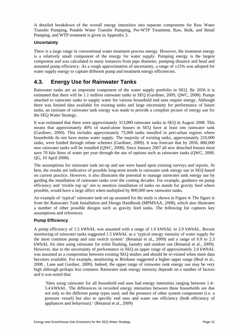
4.3. Energy Use for Rainwater Tanks Rainwater tanks are an important component of the water supply portfolio in SEQ. By 2056 it is estimated that there will be 1.1 million rainwater tanks in SEQ (Gardiner, 2009, QWC, 2008). Pumps attached to rainwater tanks to supply water for various household end uses require energy. Although there was limited data available for existing tanks and large uncertainty for performance of future tanks, an estimate of rainwater tank energy was made to provide a complete picture of energy use for the SEQ Water Strategy.
It was estimated that there were approximately 313,000 rainwater tanks in SEQ in August 2008. This means that approximately 40% of stand-alone houses in SEQ have at least one rainwater tank (Gardiner, 2009). This includes approximately 75,000 tanks installed in peri-urban regions where households do not have mains water supply. The majority of existing tanks, approximately 210,000 tanks, were funded through rebate schemes (Gardiner, 2009). It was forecast that by 2056, 800,000 new rainwater tanks will be installed (QWC, 2008). Since January 2007 all new detached houses must save 70 kilo litres of water per year through the use of options such as rainwater tanks (QWC, 2008, QG, 10 April 2008).
The assumptions for rainwater tank set-up and use were based upon existing surveys and reports. At best, the results are indicative of possible long-term trends in rainwater tank energy use in SEQ based on current practice. However, it also illustrates the potential to manage rainwater tank energy use by guiding the installation of rainwater tanks over the coming decades. For example, guidance on pump efficiency and ‘trickle top up’ not to mention installation of tanks on stands for gravity feed where possible, would have a large affect when multiplied by 800,000 new rainwater tanks.
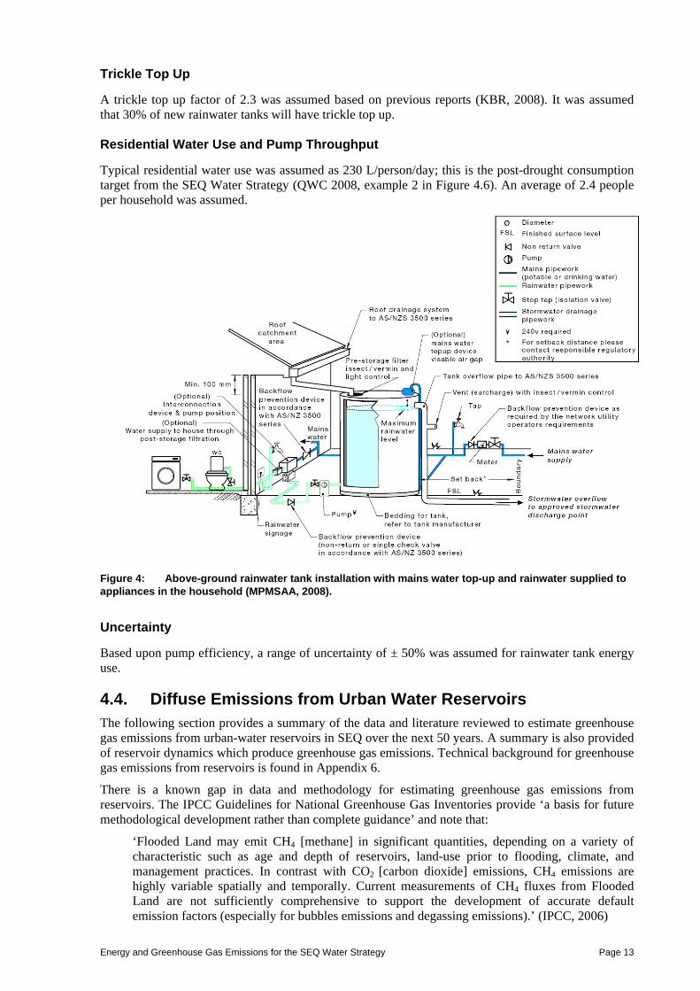
An example of ‘typical’ rainwater tank set up assumed for the study is shown in Figure 4. The figure is from the Rainwater Tank Installation and Design Handbook (MPMSAA, 2008), which also illustrates a number of other possible designs such as gravity feed tanks. The following list captures key assumptions and references.
Pump Efficiency
A pump efficiency of 1.5 kWh/kL was assumed with a range of 1.0 kWh/kL to 2.0 kWh/kL. Recent monitoring of rainwater tanks suggested 1.5 kWh/kL as a ‘typical energy intensity of water supply for the most common pump and rain switch system’ (Retamal et al., 2009) and a range of 0.9 to 2.3 kWh/kL for sites using rainwater for toilet flushing, laundry and outdoor use (Retamal et al., 2009). However, due to the uncertainty of performance in SEQ an upper range of approximately 2.0 kWh/kL was assumed as a compromise between existing SEQ studies and should be re-visited when more data becomes available. For example, monitoring in Brisbane suggested a higher upper range (Beal et al., 2008 , Lane and Gardner, 2009). Indeed, the upper range of rainwater tank energy use may be very high although perhaps less common. Rainwater tank energy intensity depends on a number of factors and it was noted that:
‘Sites using rainwater for all household end uses had energy intensities ranging between 1.4–3.4 kWh/kL. The differences in recorded energy intensities between these households are due not only to the different pump types used, and the presence of other system components (i.e. a pressure vessel) but also to specific end uses and water use efficiency (both efficiency of appliances and behaviour).’ (Retamal et al., 2009)
Energy and Greenhouse Gas Emissions for the SEQ Water Strategy Page 13
Trickle Top Up
A trickle top up factor of 2.3 was assumed based on previous reports (KBR, 2008). It was assumed that 30% of new rainwater tanks will have trickle top up. Residential Water Use and Pump Throughput
Typical residential water use was assumed as 230 L/person/day; this is the post-drought consumption target from the SEQ Water Strategy (QWC 2008, example 2 in Figure 4.6). An average of 2.4 people per household was assumed.
Figure 4: Above-ground rainwater tank installation with mains water top-up and rainwater supplied to appliances in the household (MPMSAA, 2008).
Uncertainty
Based upon pump efficiency, a range of uncertainty of ± 50% was assumed for rainwater tank energy use.
4.4. Diffuse Emissions from Urban Water Reservoirs The following section provides a summary of the data and literature reviewed to estimate greenhouse gas emissions from urban-water reservoirs in SEQ over the next 50 years. A summary is also provided of reservoir dynamics which produce greenhouse gas emissions. Technical background for greenhouse gas emissions from reservoirs is found in Appendix 6.
There is a known gap in data and methodology for estimating greenhouse gas emissions from reservoirs. The IPCC Guidelines for National Greenhouse Gas Inventories provide ‘a basis for future methodological development rather than complete guidance’ and note that:
‘Flooded Land may emit CH4 [methane] in significant quantities, depending on a variety of characteristic such as age and depth of reservoirs, land-use prior to flooding, climate, and management practices. In contrast with CO2 [carbon dioxide] emissions, CH4 emissions are highly variable spatially and temporally. Current measurements of CH4 fluxes from Flooded Land are not sufficiently comprehensive to support the development of accurate default emission factors (especially for bubbles emissions and degassing emissions).’ (IPCC, 2006)

Energy and Greenhouse Gas Emissions for the SEQ Water Strategy Page 14
Existing estimates for greenhouse gas emissions from SEQ reservoirs include the Environmental Impact Statement (EIS) for Traveston Crossing Reservoir (SKM, 2007). The EIS used the Australian Greenhouse Office National Carbon Accounting Toolbox (SKM 2007, pp10–25) and it was assumed that the main greenhouse gas was carbon dioxide. It was also assumed that the only source of carbon was the inundated land. Other inputs of carbon to the reservoir were not considered over the life of the reservoir which is a reasonable assumption for net greenhouse gas emissions if methane is not an important greenhouse gas emission from the reservoir.
‘Following construction the Project would result in a change in land use from primarily animal production and grazing to inundation. The carbon stocks associated with open grassland were estimated at 451 010 tonnes CO2 which could be released at a rate of around 5,000 tonnes CO2 per year over a number of years following inundation.’ (SKM 2007, pp10–32)
The methodology and assumptions used for estimating the greenhouse gas emissions from Traveston Crossing in the EIS are questionable and the following discussion addresses reservoir dynamics, conditions of SEQ reservoirs and existing data as the basis of a new estimate. Estimates of the mode and upper and lower ranges are also developed to capture the uncertainty due to methodology and data limitations.
Reservoirs add to the net greenhouse gas emissions in two ways. Firstly, there is a one-time breakdown of soil and plant carbon as a result of inundation when a storage fills. Secondly, reservoirs promote anaerobic conversion of organic carbon to CH4 rather than CO2 both in the water column and in the sediments. It was assumed the organic carbon would have become CO2 emission if released in a natural river channel or in the ocean in the following estimates for greenhouse gas emissions from SEQ reservoirs. As a result only the net carbon dioxide equivalent from the release of methane was considered because it is directly attributable to the conditions created by the reservoir.
Most Australian reservoirs more than 6 or 7 m deep are persistently thermally stratified during spring-autumn due to absorption of solar radiation in the water column which causes the surface waters to warm more than the deep waters. This stratification suppresses vertical transport in the water column to the extent that the interior of most reservoirs are quiescent with effective vertical diffusivities, Kz, only 10–100 times greater than molecular levels (Sherman et al. 2000). Stratification causes depletion of dissolved oxygen in deeper waters (the hypolimnion) due to respiratory demands and CO2 accumulates. When dissolved oxygen is effectively exhausted (a common occurrence) then CH4 may accumulate as well, as illustrated in Figure 5.

Energy and Greenhouse Gas Emissions for the SEQ Water Strategy Page 15
�����
��������
�� �������������
����������������������������������������
���������������������
��!"������#������
�
�
� ���������
���������������������$���
������
��������
�
��
����������� ����������
#����������������������������������
�����������������������
���������������������$���
�� �������������
�����
������
Figure 5: Conceptual model of CO2 (top) and CH4 (bottom) cycles in reservoirs (figure from Sherman et al. 2001).
Approximation of reservoir methane drew upon available, SEQ, Australian and international data. However, there was limited data available and most reservoir GHG emission studies have been conducted in North America, Europe and Brazil, with the most detailed studies relating to boreal and tropical systems. A paucity of information regarding temperate climate storages was highlighted by the World Commission on Dams (WCD 2000) and this situation has changed little since the WCD report was released. The Asia-Pacific region, which has over 60% of the world’s large dams, has virtually no studies of emissions. The only data available includes recent measurements undertaken in Tasmania and in some of the Snowy Hydro reservoirs plus a few data points from Dartmouth and Chaffey Dams as reported by Sherman et al. (2001) and recent measurements undertaken by Grinham (pers. comm. 2009) at three storages in SEQ. Figure 6 shows high spatial (and possibly temporal) variability in emissions from Wivenhoe Dam. The existing reservoir methane emission data for Australian storages is given in Table 5. Insufficient measurements have been made to accurately assess seasonal variability in emissions within a reservoir.

Energy and Greenhouse Gas Emissions for the SEQ Water Strategy Page 16
Figure 6: Methane emissions from Wivenhoe Dam. Figure courtesy A. Grinham, University of Queensland.
Table 5: Measured methane emissions from Australian reservoirs.
CH4 mg m2 d-1
Notes Location
low med high Wivenhoe
(n > 8) 24 40 73 Chamber data from A. Grinham, University of
Queensland.
Borumba (n = 1)
80 Chamber data from A. Grinham, University of Queensland.
Little Nerang (n = 3)
1,000 Chamber data from A. Grinham, University of Queensland.
Chaffey Dam (n = 2)
38 220 1,760 Profile data, flux-gradient from Sherman et al. (2001)
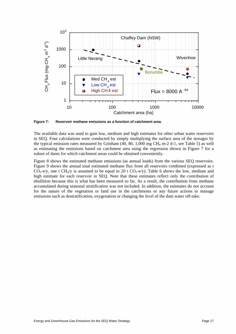
Small dams may also be relatively large greenhouse gas contributors suggesting the need to consider all urban water reservoirs and not just a few of the very largest reservoirs. Figure 7 shows a possible relationship between the catchment area and methane.
Energy and Greenhouse Gas Emissions for the SEQ Water Strategy Page 17
1
10
100
1000
104
10 100 1000 10000
Med CH4 est
Low CH4 est
High CH4 estCH
4 Flu
x (m
g-C
H4 m
-2 d
-1)
Catchment area (ha)
Little Nerang
Chaffey Dam (NSW)
Borumba
Wivenhoe
Flux = 8000 A-.64
Figure 7: Reservoir methane emissions as a function of catchment area.
The available data was used to gain low, medium and high estimates for other urban water reservoirs in SEQ. Four calculations were conducted by simply multiplying the surface area of the storages by the typical emission rates measured by Grinham (40, 80, 1,000 mg CH4 m-2 d-1, see Table 5) as well as estimating the emissions based on catchment area using the regression shown in Figure 7 for a subset of dams for which catchment areas could be obtained conveniently.
Figure 8 shows the estimated methane emissions (as annual loads) from the various SEQ reservoirs. Figure 9 shows the annual total estimated methane flux from all reservoirs combined (expressed as t CO2-e/y, one t CH4/y is assumed to be equal to 20 t CO2-e/y). Table 6 shows the low, medium and high estimate for each reservoir in SEQ. Note that these estimates reflect only the contribution of ebullition because this is what has been measured so far. As a result, the contribution from methane accumulated during seasonal stratification was not included. In addition, the estimates do not account for the nature of the vegetation or land use in the catchments or any future actions to manage emissions such as destratification, oxygenation or changing the level of the dam water off-take.

Energy and Greenhouse Gas Emissions for the SEQ Water Strategy Page 18
1
10
100
1000
104
EN
OG
GE
RA
GO
LD C
RE
EK
LAK
E M
AN
CH
ES
TE
R
EW
EN
MA
DD
OC
K
BA
RO
ON
PO
CK
ET
Hin
ze D
am
Litt
le N
eran
g D
am
CO
OLO
OLA
BIN
WA
PP
A
SIX
MIL
E
LES
LIE
HA
RR
ISO
N
SID
ELI
NG
CR
EE
K
Som
erse
t
Nor
th P
ine
Dam
Wiv
enho
e
Tra
vest
on C
ross
ing
Wya
ralo
ng
CO
OB
Y C
RE
EK
PE
RS
EV
ER
AN
CE
CR
ES
SB
RO
OK
Ma
roo
n D
am
MO
OG
ER
AH
BIL
L G
UN
N
AT
KIN
SO
N
CLA
RE
ND
ON
BO
RU
MB
A
CH
4 em
issi
on (
tonn
es-C
H4 y
-1)
Figure 8: Estimated methane emissions from reservoirs in South-East Queensland. Green bars denote medium emissions estimated using the emission level (80 mg CH4 m
-2 d-1) from Borumba dam. Orange bars denote emissions computed using catchment area-specific emission regression from Figure 7.
0
500000
1000000
1500000
2000000
2500000
low medium high area-specific Totalnon-reservoir
t - C
O2-
e / y
Figure 9: Total estimated annual methane flux (expressed as CO2-e) from SEQ reservoirs for low, medium and high areal emission rates and using the catchment area-specific regression to determine the emission rate.
Energy and Greenhouse Gas Emissions for the SEQ Water Strategy Page 19
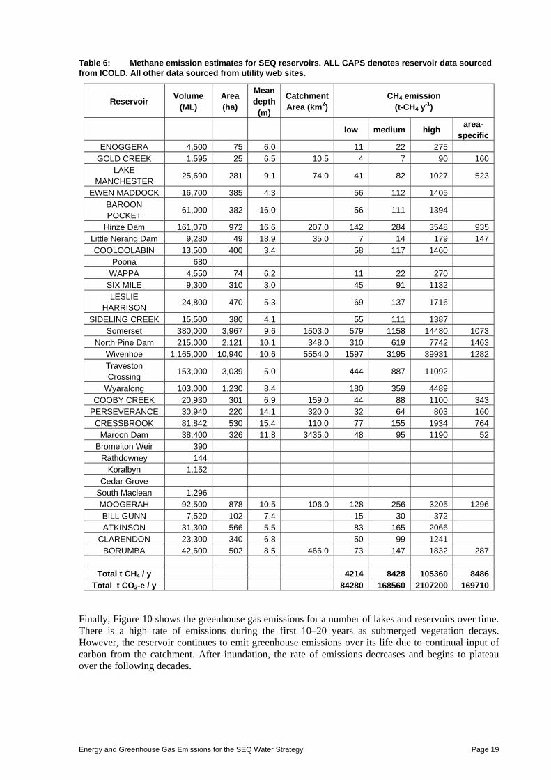
Table 6: Methane emission estimates for SEQ reservoirs. ALL CAPS denotes reservoir data sourced from ICOLD. All other data sourced from utility web sites.
Reservoir Volume
(ML) Area (ha)
Mean depth
(m)
Catchment Area (km2)
CH4 emission (t-CH4 y
-1)
low medium high area-
specific ENOGGERA 4,500 75 6.0 11 22 275
GOLD CREEK 1,595 25 6.5 10.5 4 7 90 160 LAKE
MANCHESTER 25,690 281 9.1 74.0 41 82 1027 523
EWEN MADDOCK 16,700 385 4.3 56 112 1405 BAROON POCKET
61,000 382 16.0 56 111 1394
Hinze Dam 161,070 972 16.6 207.0 142 284 3548 935 Little Nerang Dam 9,280 49 18.9 35.0 7 14 179 147 COOLOOLABIN 13,500 400 3.4 58 117 1460
Poona 680 WAPPA 4,550 74 6.2 11 22 270
SIX MILE 9,300 310 3.0 45 91 1132 LESLIE
HARRISON 24,800 470 5.3 69 137 1716
SIDELING CREEK 15,500 380 4.1 55 111 1387 Somerset 380,000 3,967 9.6 1503.0 579 1158 14480 1073
North Pine Dam 215,000 2,121 10.1 348.0 310 619 7742 1463 Wivenhoe 1,165,000 10,940 10.6 5554.0 1597 3195 39931 1282 Traveston Crossing
153,000 3,039 5.0 444 887 11092
Wyaralong 103,000 1,230 8.4 180 359 4489 COOBY CREEK 20,930 301 6.9 159.0 44 88 1100 343
PERSEVERANCE 30,940 220 14.1 320.0 32 64 803 160 CRESSBROOK 81,842 530 15.4 110.0 77 155 1934 764
Maroon Dam 38,400 326 11.8 3435.0 48 95 1190 52 Bromelton Weir 390
Rathdowney 144 Koralbyn 1,152
Cedar Grove South Maclean 1,296 MOOGERAH 92,500 878 10.5 106.0 128 256 3205 1296 BILL GUNN 7,520 102 7.4 15 30 372 ATKINSON 31,300 566 5.5 83 165 2066
CLARENDON 23,300 340 6.8 50 99 1241 BORUMBA 42,600 502 8.5 466.0 73 147 1832 287
Total t CH4 / y 4214 8428 105360 8486
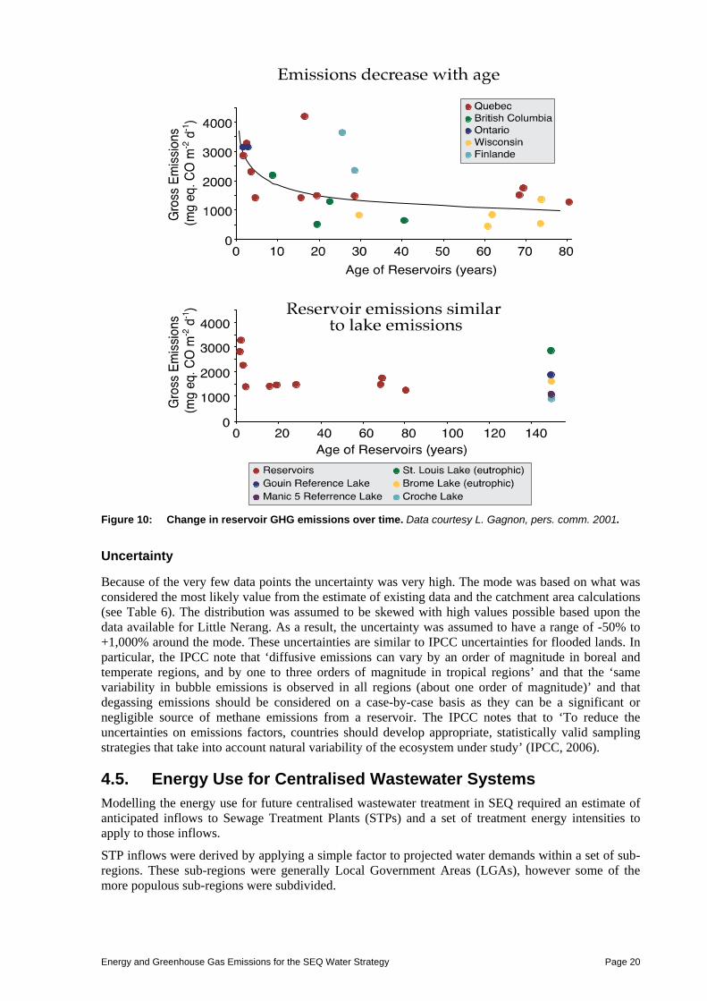
Total t CO2-e / y 84280 168560 2107200 169710 Finally, Figure 10 shows the greenhouse gas emissions for a number of lakes and reservoirs over time. There is a high rate of emissions during the first 10–20 years as submerged vegetation decays. However, the reservoir continues to emit greenhouse emissions over its life due to continual input of carbon from the catchment. After inundation, the rate of emissions decreases and begins to plateau over the following decades.
Energy and Greenhouse Gas Emissions for the SEQ Water Strategy Page 20
Figure 10: Change in reservoir GHG emissions over time. Data courtesy L. Gagnon, pers. comm. 2001.
Uncertainty
Because of the very few data points the uncertainty was very high. The mode was based on what was considered the most likely value from the estimate of existing data and the catchment area calculations (see Table 6). The distribution was assumed to be skewed with high values possible based upon the data available for Little Nerang. As a result, the uncertainty was assumed to have a range of -50% to +1,000% around the mode. These uncertainties are similar to IPCC uncertainties for flooded lands. In particular, the IPCC note that ‘diffusive emissions can vary by an order of magnitude in boreal and temperate regions, and by one to three orders of magnitude in tropical regions’ and that the ‘same variability in bubble emissions is observed in all regions (about one order of magnitude)’ and that degassing emissions should be considered on a case-by-case basis as they can be a significant or negligible source of methane emissions from a reservoir. The IPCC notes that to ‘To reduce the uncertainties on emissions factors, countries should develop appropriate, statistically valid sampling strategies that take into account natural variability of the ecosystem under study’ (IPCC, 2006).
4.5. Energy Use for Centralised Wastewater Systems Modelling the energy use for future centralised wastewater treatment in SEQ required an estimate of anticipated inflows to Sewage Treatment Plants (STPs) and a set of treatment energy intensities to apply to those inflows.
STP inflows were derived by applying a simple factor to projected water demands within a set of sub-regions. These sub-regions were generally Local Government Areas (LGAs), however some of the more populous sub-regions were subdivided.
Energy and Greenhouse Gas Emissions for the SEQ Water Strategy Page 21
Energy intensities were derived at the LGA level directly from data for existing STPs in SEQ. No attempt was made to adjust energy intensities up or down to reflect a view on how process energy efficiencies would evolve over time.
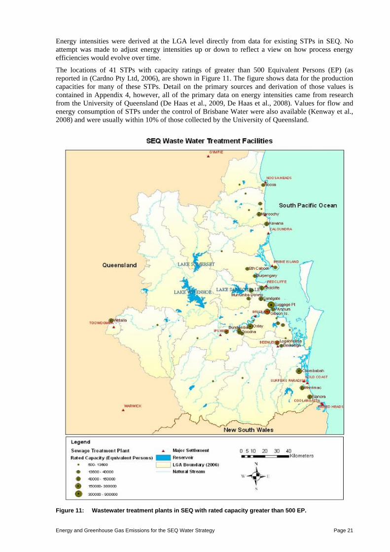
The locations of 41 STPs with capacity ratings of greater than 500 Equivalent Persons (EP) (as reported in (Cardno Pty Ltd, 2006), are shown in Figure 11. The figure shows data for the production capacities for many of these STPs. Detail on the primary sources and derivation of those values is contained in Appendix 4, however, all of the primary data on energy intensities came from research from the University of Queensland (De Haas et al., 2009, De Haas et al., 2008). Values for flow and energy consumption of STPs under the control of Brisbane Water were also available (Kenway et al., 2008) and were usually within 10% of those collected by the University of Queensland.
Figure 11: Wastewater treatment plants in SEQ with rated capacity greater than 500 EP.

Energy and Greenhouse Gas Emissions for the SEQ Water Strategy Page 22
Table 7 summarises the sewage treatment and pumping energy intensities. A flow-weighted average of energy intensity was assumed where one or more STPs currently exist in a LGA and data on STP inflows and energy use were available. Otherwise, the default value used for a sub-region was the arithmetic mean of all STPs of ‘biological treatment type 1’ (see Appendix 4) for all SEQ. Data on the sewage pumping energy was available for Brisbane and the Gold Coast (Kenway et al., 2008). Elsewhere, the arithmetic average of sewage pumping energy from those two surveys was used.
Table 7: Sewage treatment and pumping energy intensities for reticulated urban demand.
The following figures (courtesy of David de Haas, University of Queensland) explore the relationship between STP capacity and energy intensity. Economies of energy use appear to be achieved with increasing size (Figures 12 and 13). However, the spread is quite large and the size of the plant is not necessarily an indicator of low-energy intensity. For example, the most energy efficient plant appears to be of moderate size and there are a number of moderate size plants that perform as well, if not better than the largest plants. Energy for lift pumps was considered and appears to be only a relatively small contributor for gross treatment plant energy. A regression was used to understand the correlation and to develop confidence intervals which were used for estimating uncertainty in the results. A range of ± 15% was used as the range of uncertainty in the results for centralised wastewater energy.
Finally, Figure 14 illustrates plants with anaerobic digesters and power generation from biogas in comparison to other STPs. The three plants with anaerobic digesters have energy intensities higher than the mean STP energy intensity while the three anaerobic plants with cogeneration perform both above and below the mean for all STPs reported. Refer to the Appendix 5 for additional detail on treatment energy intensities and STP technology/characteristics.
Sub-Regions Data for STP(s) at LGA
level used?
STP Treatment Energy Intensity
(MWh/ML)
Sewage Pumping Energy
(MWh/ML) Cooloola No 0.71 0.20 Noosa Yes 0.69 0.20 Maroochy Yes 0.76 0.20 Caloundra No 0.71 0.20 Caboolture Yes 0.76 0.20 Redcliffe No 0.71 0.20 Toowoomba No 0.71 0.20 Boonah No 0.71 0.20 Gold Coast - North Yes 0.70 0.27 Gold Coast - South Yes 0.70 0.27 Logan No 0.71 0.20 Beaudesert No 0.71 0.20 Redland Yes 0.82 0.20 Brisbane - East Yes 0.57 0.13 Brisbane - North Yes 0.57 0.13 Brisbane - West Yes 0.57 0.13 Pine No 0.71 0.20 Esk No 0.71 0.20 Gatton No 0.71 0.20 Kilcoy No 0.71 0.20 Ipswich No 0.71 0.20 Laidley No 0.71 0.20

Energy and Greenhouse Gas Emissions for the SEQ Water Strategy Page 23
Figure 12: Gross plant power (flow-specific) including lift pumps and UV vs ADWF.
Figure 13: Corrected plant power (flow-specific), excluding lift pumps, vs. current ADWF.

Energy and Greenhouse Gas Emissions for the SEQ Water Strategy Page 24
Figure 14: Corrected plant power (flow-specific), excluding lift pumps.
Uncertainty
A range of uncertainty of ± 15% was adopted for STP energy.
4.6. Energy Use for On-Site Wastewater Systems The aim was to provide an estimate of energy use for existing as well as forecast household-scale wastewater treatment.
The number of existing on-site or decentralised wastewater systems was estimated from a review of on-site wastewater in SEQ (Beal et al., 2003). In 2003 there were approximately 127,000 decentralised wastewater systems in SEQ, with 80% of these systems being septic tanks and the remainder were aerobic systems. The number of on-site systems is projected to grow over the 10 year period from 2003–2013 to 177,000 systems and aerobic systems coupled to a septic tank favoured over just the installation of a septic tank. In the long term, the Regional Plan (QG, 2008) suggests limited growth in rural residential areas and it was assumed that there would be 204,000 on-site systems by 2056.
The energy use for decentralised systems depends upon the type of system and aerated systems generally have much higher energy use than septic tanks. Table 8 shows the assumed energy intensities for various decentralised wastewater systems.
Table 8: Decentralised wastewater system energy intensities.
Type of decentralised system Energy intensity
(kWh/kL)
Non-split septic 0
Split septic 0.22
AWTS 2.22
Sand filter 0.53

Energy and Greenhouse Gas Emissions for the SEQ Water Strategy Page 25
Uncertainty
There was very little data available to estimate uncertainty so it was assumed that the performance of small-scale decentralised wastewater systems would be sensitive to the same issues affecting rainwater tanks. An uncertainty range of ±50% was assumed.
Finally, there is considerable uncertainty with the estimate of the number and type of on-site wastewater systems in the future. The uncertainty for the scenario was not considered in this report.
4.7. Diffuse Emissions from Centralised Wastewater Systems This section quantifies the range of likely greenhouse gas emissions from diffuse sources from wastewater treatment and handling. Sources of diffuse nitrous oxide emissions considered were biosolids and the denitrification process in sewage treatment plants (STPs). Sources of diffuse methane emissions considered were biosolids and emissions from the sewerage system due to dissolved methane. All methane emissions from the anaerobic digestion process at the STP were assumed to be captured. A high and low range was developed to reflect the range of uncertainty.
The following estimates drew heavily upon the expertise and publications of the University of Queensland for diffuse methane and nitrous oxide emissions from wastewater systems, in particular the work of (Foley and Lant, 2007, Foley et al., 2008). It also drew upon the detailed data collection for SEQ wastewater plants which applied the University of Queensland methodology for diffuse wastewater emissions (De Haas et al., 2009, De Haas et al., 2008).
Methane (CH4) and nitrous oxide (N2O) emissions are potent greenhouse gases and small quantities can have a large affect on greenhouse gas emissions from a system. Both species are released from wastewater systems as ‘fugitive’ or diffuse emissions. Such emissions have generally received less attention in the past, perhaps due to lack of information rather than their contribution to greenhouse gas emissions in wastewater systems. Diffuse emissions may occur at a number of points within a system which may also complicate greenhouse gas reporting which follows organisational boundaries. The following results avoid organisational constraints by reporting for the system as a whole.
Methane is produced in wastewater systems by anaerobic metabolism of organic material by microorganisms. This largely occurs in treatment plant reactors which offer the potential to capture methane released to the gas phase. However, a fraction of the dissolved methane may remain in the effluent, especially for ‘weak’ domestic wastewater flows, which may be released downstream in processes such as lagoons (Foley and Lant, 2007).
Nitrous oxide is produced in sewage treatment plants with biological nutrient removal (BNR) processes. Nitrous oxide is a by-product or intermediary when converting organic nitrogen and ammonium into nitrogen gas and is likely to be released to the atmosphere due to mass transfer and process constraints (Foley and Lant, 2007).
The disposal of biosolids can also produce methane and nitrous oxide emissions. For mass transfer and process details for both diffuse emissions refer to (Foley and Lant, 2007). The appendices contain an extract from work published by the University of Queensland (De Haas et al., 2009) which provides further details of plants considered, emission factors and other assumptions.
Uncertainty
The uncertainty for emission factors for diffuse wastewater emissions is very large. In general, the emission factors are based upon literature from various countries. The conditions considered in the studies are often quite different (such as hot and cold climates) and processes are not equally documented. In some cases, such as methane emissions from raw wastewater, the IPCC does not provide any formal guidance.
Nitrous oxide emissions In general the uncertainty for nitrous oxide emissions is large. The IPCC emission factor for nitrogen to nitrous oxide for wastewater treatment has an uncertainty range of 50% to 200% and is based upon a single reference. The IPCC assumes 1% of nitrogen is converted to nitrous oxide emissions but this also includes emissions outside of the treatment works. The UK Water Industry Research (UKWIR)

Energy and Greenhouse Gas Emissions for the SEQ Water Strategy Page 26
assumes an uncertainty of 30% to 300% based upon a review of ten sources (Andrews et al., 2008) and assumes 0.003 kgN2O-N/kgN (0.002* N load on secondary treatment*44/28 – Equation 2). In a review of 11 sources, (Foley and Lant, 2007) estimate a range of 0.00029 to 0.03 kgN2O-N/kgN influent for wastewater treatment with the median being 0.01 kgN2O-N/kgN influent. The assumed emission factor for nitrous oxide emissions from treatment was 0.01 kg N2O-N/kgN influent with an uncertainty range of -50% to +300%.
There is also large uncertainty for nitrous oxide emissions from biosolids. The emission factor recommended by (Foley and Lant, 2007) was 0.011 kgN2O-N/kgN applied (which was the median value of the 11 references reviewed). This was similar to the IPCC value of 0.01 kgN2O-N/kgN for applying ‘mineral fertilisers, organic amendments and crop residues’ for managed soils with an uncertainty range of 0.003 to 0.03 kgN2O-N/kgN (IPCC, 2006). The UKWIR assumes an emission factor of 0.006 kgN2O-N/kgN (assuming 0.043 kgN/kg dry sludge and an emission factor of 0.26 kgN2O-N/tonne dry sludge) (Andrews et al., 2008). A detailed field study in SEQ indicated that nitrous oxide emissions could be significant and be affected by factors such as application rates and wetness of the soil which in turn was affected by polymers in the biosolids dewatering processes.
‘Laboratory studies showed that gaseous N losses were significant (up to 40% of organic N in a 100 day incubation period) and although NH3 volatilisation was detected, by far the dominant loss pathway being denitrification of N2/N2O. Results showed that losses were greatest in wet soil conditions and exacerbated by the presence of the polymers used in biosolids dewatering processes. Field and laboratory/glasshouse experiments showed that these gaseous losses could be greatly reduced by reducing the biosolids application rates or by continuous rapid uptake of mineral N by plants (e.g. in cut and remove forage cropping).’ (Barry and Bell, 2006)
In summary, an emission factor of 0.011 kgN2O-N/kg sludge N which is the same as assumed by (Foley et al., 2008) with an uncertainty range of -50% to +300% was adopted for nitrous oxide emissions from biosolids.
Nitrous oxide emissions from effluent disposed to receiving waters can also be complicated by the accounting rules for greenhouse gas emissions. The UKWIR tool does not consider nitrous oxide emissions from wastewater effluent because it argues that the N load would have entered the receiving waters regardless of the sewage treatment plant (Andrews et al., 2008). However, in this study these emissions are included because the aim is to provide a measure of the total greenhouse emissions independent of who is responsible for them. An uncertainty range of -50% to +300% was also adopted for this source of nitrous oxide emissions.
Methane
Uncertainty in the emission factors for methane was also very large. For primary and secondary treatment (anaerobic lagoons, high-rate anaerobic reactors and facultative lagoons) the uncertainty in emission factors is approximately 50% based upon literature reviewed by (Foley and Lant, 2007).
However, for other emission factors for diffuse methane emissions the literature provides a large range of values. For terrestrial receiving environments including landfill, agricultural and stockpiling of biosolids there was a large range in reported values and in some cases no literature at all (Foley and Lant, 2007). The UKWIR assumed a sludge to landfill uncertainty of ±60% based largely on information from personal communication for application in a cold climate (Andrews et al., 2008). Consequently, an uncertainty range of ±50% was assumed. However, this assumption should be reviewed when more data becomes available.
A ± 50% uncertainty was also applied to the methane emissions from the sewer due to the lack of data.
4.8. Diffuse Emission from On-Site Wastewater Systems ‘Chapter 6 – Wastewater Treatment and Discharge’ of the ‘2006 IPCC Guidelines for National Greenhouse Gas Inventories’ (referred to as the IPCC Guidelines in this section) was used to develop an estimate of methane emissions from on-site anaerobic systems. The IPCC Guidelines note that direct nitrous oxide emissions only need to be estimated for countries that have ‘predominantly advanced centralized wastewater treatment plants with nitrification and denitrification steps’. (IPCC, 2006). This assumption appears reasonable given that on-site systems do not have denitrification

Energy and Greenhouse Gas Emissions for the SEQ Water Strategy Page 27
processes, the default emission factor for sludge is zero and there is currently insufficient information to demonstrate emissions from discharge by irrigation (Foley and Lant, 2007). An initial estimate of nitrous oxide emissions from biosolids showed it to be only a couple of percent of the on-site methane emissions and was not considered further. Carbon dioxide emissions from wastewater were not included following the IPCC Guideline approach that they are of biogenic origin and should not be included in total emissions (IPCC 2006). These assumptions may need to be revisited in the future.
Details of the on-site wastewater methane calculation are given in Appendix 8.
Uncertainty
Uncertainty of ± 50% was assumed for methane emissions. This uncertainty is the same as assumed for centralised wastewater methane emissions and is similar to uncertainties reported in Table 6.7 of the IPCC Guidelines for the parameters in the above calculations (IPCC 2006; see also Appendix 8). For example, the maximum CH4 producing capacity (Bo) has an uncertainty of ± 30%, the fraction treated anaerobically (MCF) has an uncertainty up to ± 50% and the BOD (biochemical oxygen demand) has an uncertainty of ± 30%.
Finally, there is considerable uncertainty with the estimate of the number and type of on-site wastewater systems in the future. The uncertainty for the scenario is not considered in this report. Refer to section 4.6 Energy Use for On-Site Wastewater Systems for details of decentralised wastewater system numbers.
5. ENERGY AND GREENHOUSE GAS EMISSIONS FOR THE DRAFT SEQ WATER STRATEGY
5.1. Energy
5.1.1. Calibration to the Draft SEQ Water Strategy
The minimum energy for supply calculated for this project was similar to results in the draft SEQ Water Strategy. This was not surprising given the project assumed the same demand-supply balance as the Strategy. However, there were a number of different assumptions for the operating regime. To create a minimum energy curve it was assumed that the lowest energy source of water would be used first. It was also assumed that high-energy sources such as desalination plants would not be turned off but operated at minimum turn down levels. The latter assumption was made to follow anticipated operating regimes for desalination plants once commissioned. Further reductions in the minimum energy reported below could be achieved, for example, if desalination plants are turned off completely when not required. The SEQ Water Strategy assumes that all available supplies are used at a proportion of overall system demand to overall system capacity. As a result, the SEQ Water Strategy uses desalinisation plants before other lower energy supplies are used to full capacity. In addition, the proportion of water from sources such as desalination may not be technically possible if used at levels below the minimum turn-down. Figure 15 illustrates the project results for minimum energy use from the SEQWS, shown in orange, superimposed over Figure 6.13 from the Draft SEQ Water Strategy (QWC 2008). Although the overall trend is increasing energy use over time, the minimum energy curve has small steps down in energy use when a low-energy supply source becomes available and is substituted for higher-energy sources.

Energy and Greenhouse Gas Emissions for the SEQ Water Strategy Page 28
Figure 15: Comparison of energy for grid water to the draft SEQ Water Strategy (figure 6.13 from QWC 2008).
5.1.2. Energy for Water and Wastewater
Figure 16 illustrates that the total energy for water and wastewater will increase many times over in the next 50 years. Energy for water supply approximately triples over the next 50 years and increases at a faster rate than wastewater energy due to the use of energy-intensive supplies such as desalination. The initial jump in energy use for the system is due to the commencement of operation of the SEQ Desalination Plant (Tugun). In contrast, energy to treat a unit of wastewater will not increase significantly and the total wastewater energy follows the increase in flow due to increased population. The water and wastewater curves include centralised and decentralised systems and the combined uncertainty is shown by the dotted lines.
0
200000
400000
600000
800000
1000000
1200000
1400000
1600000
2008
2011
2014
2017
2020
2023
2026
2029
2032
2035
2038
2041
2044
2047
2050
2053
2056
YEAR
EN
ER
GY
(M
Wh
)
WATER WASTEWATER
Figure 16: Energy for water and wastewater. Uncertainties are shown with dashed lines and using the same colour as the mode.
Minimum energy required for bulk water
supply calculated in this project
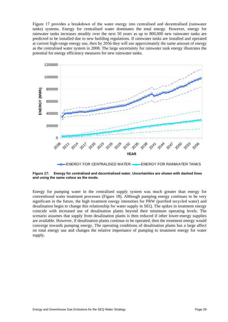
Energy and Greenhouse Gas Emissions for the SEQ Water Strategy Page 29
Figure 17 provides a breakdown of the water energy into centralised and decentralised (rainwater tanks) systems. Energy for centralised water dominates the total energy. However, energy for rainwater tanks increases steadily over the next 50 years as up to 800,000 new rainwater tanks are predicted to be installed due to new building regulations. If rainwater tanks are installed and operated at current high-range energy use, then by 2056 they will use approximately the same amount of energy as the centralised water system in 2008. The large uncertainty for rainwater tank energy illustrates the potential for energy efficiency measures for new rainwater tanks.
0
200000
400000
600000
800000
1000000
1200000
2008
2011
2014
2017
2020
2023
2026
2029
2032
2035
2038
2041
2044
2047
2050
2053
2056
YEAR
EN
ER
GY
(M
Wh
)
ENERGY FOR CENTRALISED WATER ENERGY FOR RAINWATER TANKS
Figure 17: Energy for centralised and decentralised water. Uncertainties are shown with dashed lines and using the same colour as the mode.
Energy for pumping water in the centralised supply system was much greater than energy for conventional water treatment processes (Figure 18). Although pumping energy continues to be very significant in the future, the high treatment energy intensities for PRW (purified recycled water) and desalination begin to change this relationship for water supply in SEQ. The spikes in treatment energy coincide with increased use of desalination plants beyond their minimum operating levels. The scenario assumes that supply from desalination plants is then reduced if other lower-energy supplies are available. However, if desalination plants continue to be operated, then the treatment energy would converge towards pumping energy. The operating conditions of desalination plants has a large affect on total energy use and changes the relative importance of pumping to treatment energy for water supply.

Energy and Greenhouse Gas Emissions for the SEQ Water Strategy Page 30
0
100000
200000
300000
400000
500000
600000
700000
800000
2008
2011
2014
2017
2020
2023
2026
2029
2032
2035
2038
2041
2044
2047
2050
2053
2056
YEAR
EN
ER
GY
(M
Wh
)
PUMPING ENERGY TREATMENT ENERGY
Figure 18: Comparison of energy use for centralised water pumping and treatment. Uncertainties are shown with dashed lines and using the same colour as the mode.
Centralised wastewater energy use is much greater than for decentralised (on-site) wastewater systems (Figure 19). Decentralised wastewater systems represent about a sixth of the total wastewater energy by 2056. It is estimated that the rate of SEQ-wide energy use for decentralised systems will decrease after about a decade. However, even if the number of decentralised systems were doubled from the assumed scenario shown below, decentralised wastewater systems would still consume much less energy than the centralised system.
0
100000
200000
300000
400000
500000
600000
2008
2011
2014
2017
2020
2023
2026
2029
2032
2035
2038
2041
2044
2047
2050
2053
2056
YEAR
EN
ER
GY
(M
Wh
)
ENERGY FOR CENTRALISED WASTEWATER ENERGY FOR ON-SITE WASTEWATER
Figure 19: Energy for centralised and decentralised wastewater. Uncertainties are shown with dashed lines and using the same colour as the mode.

Energy and Greenhouse Gas Emissions for the SEQ Water Strategy Page 31
5.2. Greenhouse Gas Emissions This section presents results of greenhouse gas (GHG) emissions for the SEQ urban water and wastewater systems. It builds upon the data presented for energy by calculating the greenhouse gas emissions for energy supply as well as adding emissions from diffuse sources.
5.2.1. Greenhouse Gas Emissions for Water and Wastewater
Figure 20 compares the greenhouse gas emissions for water and wastewater systems. The large range reflects the large uncertainties for diffuse emissions. Water emissions have a very large upper range due to uncertainties with methane emissions from reservoirs. Wastewater systems also have a very large upper range for diffuse nitrous oxide and methane emissions. The overlap of the upper ranges of the uncertainties illustrate that it is possible that either water or wastewater could be the dominant source of greenhouse gas emissions despite their modes. This illustrates that such high uncertainty needs to be addressed before further analysis can be undertaken. The general upward trend reflects an increase in population although this too is relatively small compared to the uncertainty from diffuse emissions.
0
500000
1000000
1500000
2000000
2500000
3000000
3500000
2008
2011
2014
2017
2020
2023
2026
2029
2032
2035
2038
2041
2044
2047
2050
2053
2056
YEAR
GR
EE
NH
OU
SE
GA
S E
MIS
SIO
NS
(to
nn
e C
O2-
e)
WATER WASTEWATER
Figure 20: Greenhouse gas emissions for water and wastewater. Uncertainties are shown with dashed lines and using the same colour as the mode.
5.2.2. Breakdown of Greenhouse Gas Emissions for Water Supply
Figure 21 disaggregates the total greenhouse gas emissions presented for the water supply in Figure 20. The mode for reservoir methane is relatively low and over time is smaller than centralised water and rainwater tank greenhouse gas emissions. However, the uncertainty for the upper range of reservoir methane emission is high and this dominates the combined uncertainty for the water greenhouse gas emissions.
Rainwater tank uncertainty is also large and follows the uncertainty outlined for rainwater tank energy use (see Figure 17).

Energy and Greenhouse Gas Emissions for the SEQ Water Strategy Page 32
0
200000
400000
600000
800000
1000000
1200000
1400000
1600000
1800000
2000000
2008
2011
2014
2017
2020
2023
2026
2029
2032
2035
2038
2041
2044
2047
2050
2053
2056
YEAR
GR
EE
NH
OU
SE
GA
S E
MIS
SIO
NS
(to
nn
e C
O2-
e)
RAINWATER TANKS RESERVOIR METHANE CENTRALISED WATER
Figure 21: Breakdown of water supply greenhouse gas emissions. Uncertainties are shown with dashed lines and using the same colour as the mode.
5.2.3. Breakdown of Greenhouse Gas Emissions for Wastewater
The mode for greenhouse gas emissions for centralised wastewater energy use is much greater than for diffuse emissions (Figure 22). However, there is large uncertainty for diffuse emissions and the high range estimate is greater than both the mode and upper range estimate for greenhouse gas emissions from wastewater energy use. On-site wastewater GHG emissions are much less than centralised wastewater emissions. The modes for greenhouse gas emissions from on-site energy and diffuse emissions are very similar as are the uncertainty ranges.
Energy and Greenhouse Gas Emissions for the SEQ Water Strategy Page 33
0
100000
200000
300000
400000
500000
600000
2008
2010
2012
2014
2016
2018
2020
2022
2024
2026
2028
2030
2032
2034
2036
2038
2040
2042
2044
2046
2048
2050
2052
2054
2056
YEAR
GR
EE
NH
OU
SE
GA
S E
MIS
SIO
NS
(to
nn
e C
O2-
e)
ON-SITE WASTEWATER ENERGYON-SITE WASTERWATER METHANECENTRALISED WASTEWATER ENERGYCENTRALISED WASTEWATER DIFFUSE EMISSIONS
Figure 22: Breakdown of wastewater greenhouse gas emissions. Uncertainties are shown with dashed lines and using the same colour as the mode.
5.3. Sensitivity of Energy and Greenhouse Gas Emissions to Reduced Demand
The aim of this section was to explore the sensitivity of centralised water energy use to changes in demand. This analysis reveals aspects of system performance as well as limitations of the current approach and areas for further research.
It was assumed that per capita residential demand was reduced from 230 litres per person per day (L/p/d), used in the SEQ Water Strategy, to 170 L/p/d. This is approximately a 25% reduction in demand and has significant ‘level of service’ and demand management implications. The realism of such a reduction is not considered in this section. The water balance was recalculated to maintain the conditions of demand not greater than supply and a drought supply requirement below 180,000 ML/annum (QWC 2008, p141). The Draft SEQ Water Strategy notes for a 230 L/p/d demand that:
‘In a drought scenario and without additional supply capacity beyond the committed projects, it is expected that the drought supply requirement will exceed 180,000 ML/a for the first time between 2034 and 2044. From this time, the need for additional climate resilient supplies would be expected to drive the selection of infrastructure required to meet the needs in normal conditions and at the same time to ensure that the Drought Response Plan is practical to implement’. (QWC 2008, p141)
Reducing demand below 230 L/p/d has the effect of delaying when the drought supply requirement will exceed 180,000 ML/a assuming the supply capacity of the committed projects. As a result, a number of ‘climate resilient’ supplies were not required to meet the 170 L/p/d demand after 2040 and up to 2056.

Energy and Greenhouse Gas Emissions for the SEQ Water Strategy Page 34
There are a number of limitations to the following results. The calculations were performed on an annual time step and day-to-day dynamics within the system were not captured. For example, a reduced demand could reduce the volume of inter-basin transfers within each year. Such dynamics were not well captured in the annual time step. In addition, short-term increases in the operation of desalination plants during the year are not well captured. Such a situation is possible if there is large variation and mismatch of demand and supply within the year. This could be improved by integrating energy data with a water balance model that better reflects the operation of the SEQ water grid.
Figure 23 illustrates that energy use for centralised water does not decrease by much more than 10% for the next 20 years despite a 25% reduction in demand. As a result, the difference between the two scenarios is within the ± 15% uncertainty range for the data for a number of decades. The relatively small reduction in energy use was due to the operating condition that high-energy desalination plants cannot be switched off completely during periods of excess water supply capacity. Rule 6.3 of the South East Queensland System Operating Plan (QWC, 2009b) states that the Goldcoast Desalination Plant will supply water at a rate of at least one-third of the production capacity of the plant. This corresponds to the minimum operating capacity of the Goldcoast Desalination Plant before it is turned off completely (Crisp, G. GHD Global Business Leader – Desalination, pers. comm. 10 January 2010). Similarly, other desalination plants were assumed to operate at their minimum turn down, such as the Sunshine Coast plant minimum turn down of 16%. The PRW plants were assumed to operate at the rate of sewage generation. Consequently, once high-energy supplies are introduced, both the relatively low demand and higher demand profiles use a proportion of the high-energy sources regardless of the availability of alternatives. This was reflected in the two demand scenarios which begin to diverge at approximately 2030 when other low-energy water supplies are no longer available and high-energy supplies need to be operated above minimum levels.
In summary, the sensitivity of centralised water energy use to reductions in demand is reduced by minimum levels of operation for high-energy water sources such as desalination. Further research is required to understand system dynamics within each year.
0
200000
400000
600000
800000
1000000
1200000
2008
2011
2014
2017
2020
2023
2026
2029
2032
2035
2038
2041
2044
2047
2050
2053
2056
YEAR
EN
ER
GY
(M
Wh
)
ENERGY FOR CENTRALISED WATER (170 l/p/d DEMAND)
ENERGY FOR CENTRALISED WATER (230 l/p/d DEMAND)
Figure 23: Sensitivity of centralised water energy use to changes in demand. Uncertainties are shown with dashed lines and using the same colour as the mode.
Energy and Greenhouse Gas Emissions for the SEQ Water Strategy Page 35
6. CONCLUSIONS
The research estimates energy use and greenhouse gas emissions for the SEQ Water Strategy. It provides the basis for setting targets as well as identifying areas for mitigation. The report considered centralised water and wastewater services, decentralised water and wastewater systems and diffuse greenhouse gas emissions.
The following list provides a summary of key results:
Energy for pumping is much greater than treatment energy for centralised water services in SEQ. Pumping currently accounts for approximately 80% of energy use for centralised water services. However, this relationship will change if desalination plants (with high treatment energy use) are operated above minimum levels.
Greenhouse gas emissions will rise faster than growth in population and will more than double for water and wastewater services in SEQ over the next 50 years. New sources of water supply such as desalination, recycled water and rainwater tanks currently have greater energy intensity than traditional sources.
The ability to turn down or turn off high-energy water supplies such as desalination is important to achieve energy savings from reduced water demand. This has important implications for plant design and System Operating Plans (SOP). For example, the current SOP requires the Goldcoast Desalination Plant be operated at a rate of at least one third of its capacity – which corresponds to the lowest level of operation of the plant before it is switched off completely. Under this operating regime, if water demand is reduced by 25%, equivalent to reducing residential demand from the permanent water conservation ‘Target 230’ litres per person per day (l/p/d) to the high restriction ‘Target 170’ l/p/d, then energy use for the system is only reduced by about 10% for the following two decades. Greater energy savings are not achieved because desalinated water is supplied even when low-energy water supplies are available.
Diffuse greenhouse gas emissions are potentially much greater than emissions from energy use for the sector; although the data currently has a very high level of uncertainty. The main sources of diffuse emissions include reservoirs as well as wastewater treatment and handling.
The 800,000 new rainwater tanks that are planned to be installed in SEQ over the next 50 years may use as much energy as the current centralised water supply if installed and operated at the upper ranges of current energy use. There is a large range in efficiency and appropriate guidance for tank set up could significantly reduce this impact.
A handful of large water and wastewater plants account for the bulk of treatment capacity in SEQ. For wastewater treatment plants, there was a weak correlation between plant size and energy efficiency.
Future directions for research and potential mitigation should focus on sources of energy use and greenhouse gas emissions that make a large contribution to system results and have high levels of uncertainty. These include diffuse greenhouse gas emissions from reservoirs and wastewater systems and energy use from rainwater tanks. In addition, the scope of the research should be expanded beyond energy use and greenhouse gas emissions to other key environmental issues for the water sector such as aquatic ecosystem impacts. Consideration of economic and social considerations would also allow an evaluation of sustainability and comparison of options.
In this context, the information presented in this report expands energy use and greenhouse gas emissions considerations for the SEQ urban water sector. It provides valuable information to help understand the sustainability challenge of water and wastewater services in SEQ over the coming decades.

Energy and Greenhouse Gas Emissions for the SEQ Water Strategy Page 36
7. REFERENCES
ANDREWS, J., HOBSON, J., HUNT, D. & SHEPHERD, D. (2008) Carbon Accounting in the UK Water Industry: Methodology for Estimating Operational Emissions, Report Ref. No. 08/CL/01/5. UK WIR.
AUSTRALIAN WATER ASSOCIATION (2005) Status of water in South East Queensland for the Courier Mail. Australian Water Association.
BARRY, G. & BELL, M. (2006) Sustainable Biosolids Recycling in South east Queensland. Qld Govt Natural Resources and Water.
BEAL, C. D., GARDNER, T., CHRISTIANSEN, C. & BEAVERS, P. (2003) A review of on-site wastewater management practices / knowledge in SEQ local governments. . IN DEPARTMENT OF NATURAL RESOURCES AND MINES, B., QLD. (Ed.
BEAL, C. D., HOOD, B., GARDNER, T., CHRISTIANSEN, C. & LANE, J. (2008 ) Energy and water metabolism of a sustainable subdivision in South East Qld: the little toe of the urban ecological footprint? . Proceedings of Enviro 08, 5-7 May 2008. Melbourne, Australia.
CARDNO PTY LTD (2006) Review of Use of Stormwater and Recycled Water As Alternative Water Resources - Draft Report. Brisbane, SEQ Regional Water Supply Strategy.
CSIRO (2007) Climate Change in Australia. CSIRO. CSIRO & BRISBANE WATER (2008) Brisbane Water - CSIRO Energy Water Project.xls. CSIRO and
Brisbane Water. CSIRO & GOLD COAST WATER (2008) Gold Coast Water - CSIRO Energy Water Project.xls. CSIRO
and Gold Coast Water. DE HAAS, D. (2008) SEQ_WWTPs inventory v2 2.xls. IN WEST, J. (Ed., Griffith University. DE HAAS, D., FOLEY, J. & LANT, P. (2009) Energy and greenhouse footprints of wastewater treatment
plants in south-east Queensland. Ozwater’09. Melbourne. DE HAAS, D. W., FOLEY, J. & BARR, K. (2008) Greenhouse gas inventories from WWTPs - the trade-
off with nutrient removal. . WEF Sustainability 2008 Conference. National Harbor, Maryland, USA. FOLEY, J. & LANT, P. (2007) Fugitive Greenhouse Gas Emissions from Wastewater Systems, WSAA
Literature Review No.01. Water Services Association Australia (WSAA). FOLEY, J., LANT, P. & DONLON, P. (2008) FUGITIVE GREENHOUSE GAS EMISSIONS FROM
WASTEWATER SYSTEMS. Water, March 2008, 18-23. GARDINER, A. (2009) Domestic rainwater tanks: usage and maintenance patterns in south east
Queensland. Water, Volume 36 151-156. GHGPROTOCOL (2001) GHG Protocol Corporate Standard, GHG Protocol guidance on uncertainty
assessment in GHG inventories and calculating statistical parameter uncertainty. GREGG, M. (2007) BW Energy 0405 CSIRO Request.xls. Brisbane Water. IPCC (2000) Good Practice Guidance and Uncertainty Management in National Greenhouse Gas
Inventories. IPCC (2006) Guidelines for National Greenhouse Gas Inventories. ISO (2006a) ISO 14040 Environmental Management - Life Cycle Assessment - Principles and Framework.
Switzerland, ISO. ISO (2006b) ISO 14044 Environmental Management - Life Cycle Assessment - Requirements and
Guidelines. Switzerland, ISO. JACOB, P. & WHITEOAK, K. (2008) Energy Intensity of the Draft SEQ Water Strategy. Marsden Jacob
Associates for Queensland Water Commission. JONES, R. N. & PRESTON, B. L. (2006) Climate Change Impacts, Risks and the Benefits of Mitigation:
A report to the Energy Futures Forum. CSIRO. KBR (2008) South East Queensland Regional Water Supply Strategy - Energy Consumption Discussion
Paper. Kellogg Brown and Root for the Queensland Water Commission. KENWAY, S. J., PRIESTLEY, A., COOK, S., SEO, S., INMAN, M., GREGORY, A. & HALL, M. (2008)
Energy use in the provision and consumption of urban water in Australia and New Zealand. CSIRO: Water for a Healthy Country National Research Flagship for the Water Services Association of Australia.
LANE, J. & GARDNER, T. (2009) A life-cycle comparison of decentralised and centralised water cycle approaches. Ozwater'09. Melbourne, Australia.
MPMSAA (2008) Rainwater Tank Design and Installation Handbook. National Water Commission, Australian Government.

Energy and Greenhouse Gas Emissions for the SEQ Water Strategy Page 37
QDNRW (2007a) MWH_STPs_Labelled#2_point_11_06. Queensland Department of Natural Resources and Water.
QDNRW (2007b) waterTreatmentPlants_wcrwp Queensland Department of Natural Resources and Water. QG (10 April 2008) Queensland Development Code MP 4.2 Water Savings Targets. Queensland
Government, Australia. QG (2008) Draft SEQ Regional Plan 2009-2031. IN PLANNING, D. O. I. A. (Ed., Queensland
Government. QWC (2008) South East Queensland Water Strategy - Draft March 2008. QWC (2009a) Queensland Water Commission, Accessed 6 February 2009,
http://www.qwc.qld.gov.au/Water+use+measurement. QWC (2009b) South East Queensland System Operating Plan, Release 2.2, 21 September 2009.
Queensland Water Commission. RETAMAL, M. L., GLASSMIRE, J., ABEYSURIYA, K. R., TURNER, A. J. & WHITE, S. (2009) The
Water-Energy Nexus: Investigation into the energy implications of household rainwater systems. Prepared for CSIRO by the Institute for Sustainable Futures, Sydney.
SKM (2007) Traveston Crossing Dam Environmental Impact Statement. IN LTD, Q. W. I. P. (Ed. WSAA (1999) Affordable Water Supply & Sewerage for small communities Report No WSAA 125. Water
Services Association of Australia.
Energy and Greenhouse Gas Emissions for the SEQ Water Strategy Page 38
APPENDIX 1. DATA DERIVATION FOR GIS LAYER OF WTPS
Detailed location data for the water treatment plants (WTPs) was obtained from the Queensland Department of Natural Resources and Water (QDNRW, 2007b), along with data on the type of plant and nominal capacities. Data on the notional peak capacity of 37 of these was also available from (Australian Water Association, 2005). As these figures appeared to include more recent data, they were substituted as defaults where available. Data on capacities and estimates of the treatment energy intensity for a subset of 11 WTPs was also given in (Jacob and Whiteoak, 2008). The capacities from that report were accepted here for all of that subset, whilst the energy intensities were used for seven of the 11. Furthermore, an arithmetic average of the energy intensities for the 11 WTPs dealt with in (Jacob and Whiteoak, 2008) was used as the default energy intensity for all WTPs where more specific data was not available.
Detailed data for energy use and water supplied for a 12-month period was available for four key WTPs (Mt Crosby East, North Pine, Mudgeeraba and Molendinar), which jointly account for over 75% of the treatment capacity in SEQ. The data was gathered in two surveys, one for Gold Coast Water’s operations (CSIRO and Gold Coast Water, 2008) another for Brisbane Water’s operations (CSIRO and Brisbane Water, 2008). This data was used in conjunction with information provided in (Gregg, 2007), on the proportion of energy used in specific plants for pumping operations, to resolve the total energy intensity of WTPs into separate components for pure water treatment activities and for pumping activities which had been aggregated into the water treatment figures. According to (Gregg, 2007), approximately 90% of the energy used for treatment at Mt Crosby is attributable to the pumping required for one lift of approximately 120m. This figure appears reasonable when checked against the formula:
Power (W) = (Head (m) x Flow (Ls-1) x Gravity (ms-2)) / Pump Efficiency
Using 2006/2007 figures of 139,007 ML treated, and 90% of the 60516 MWh used (54464 MWh), the implied pump efficiency is approximately 83%, which is reasonable for large pumps through big pipes.
For the North Pine WTP, energy used in treatment was split 60% for pumping and 40% for pure treatment processes.
Information on any similar split for the Gold Coast plants was not available; however, as the total energy for treatment recorded in the surveys is comparable to the net of pumping figure for Mt Crosby, it seems unlikely that a significant pumping component has been aggregated with the treatment energy for these WTPs.

Energy and Greenhouse Gas Emissions for the SEQ Water Strategy Page 39
APPENDIX 2. DETAILS OF DATA SOURCES FOR ENERGY INTENSITY OF MAINS WATER SUPPLY
Region Water source Supply task Treatment
+ Pumping Energy
Comments
(MWh/ML)
Borumba Dam Raw water source to local tap
0.84 Energy intensities for Borumba Dam were taken to be equal to those determined for Traveston Crossing Dam stage 1, (see Traveston Crossing Dam stage 1, below). This assumes that there is no piping/pumping energy necessary for transfers from above Traveston. Note that there is a drop of around 50m between Borumba and Traveston, which might have implications for hydro electric offsets.
Lake MacDonald Raw water source to local tap
0.39 Specific data wasn't available for Lake McDonald, so "WTP Treatment" energy intensity was determined as outlined in (1), with "Raw, Bulk, and Retail Pumping" energy intensity determined as outlined in (2).
Maroochy System (Cooloolabin & Wappa)
Raw water source to local tap
0.40 MJA figure for treatment at Image Flat WTP used for "WTP Treatment", with "Raw, Bulk, and Retail Pumping" energy intensity determined as outlined in (2).
Baroon Pocket Dam Raw water source to local tap
0.46 MJA figure for treatment at Landershute WTP used for "WTP Treatment", with "Raw, Bulk, and Retail Pumping" energy intensity determined as outlined in (2).
North Coast
Caboolture Weir Raw water source to local tap
0.39 "WTP Treatment" energy intensity was determined as outlined in (1), with "Raw, Bulk, and Retail Pumping" energy intensity determined as outlined in (2).
Ewen Maddock Dam Raw water source to local tap
0.48 MJA figure for treatment at Ewen Maddock WTP used for "WTP Treatment", with "Raw, Bulk, and Retail Pumping" energy intensity determined as outlined in (2).
Kawana Desalination Plant (1a)
Raw water source to local tap
4.28 The energy intensity for the SWRO process was derived as for Tugun (see below). "Raw, Bulk, and Retail Pumping" energy intensity determined as outlined in (2).
Kawana Desalination Plant (1b)
Raw water source to local tap
4.28 As above
North Coast PRW AWTP treatment to local tap
1.94 Pre-WTP Treatment Energy is for PRW process, and uses MJA value for Bundamba AWTP. Pumping PRW water to dam ("Raw Water Transfer Pumping") uses the MJA Sunshine Coast to Traveston Dam Stage 1 figure. "WTP Treatment" energy intensity was determined as outlined in (1), with "Raw, Bulk, and Retail Pumping" energy intensity determined as outlined in (2).
Noosa Purified Recycled Water
AWTP treatment to local tap
2.02 "Pre-WTP Treatment" energy intensity from the MJA value for Bundamba AWTP. "Raw Water Transfer Pumping" uses the MJA value for transfer from the Sunshine Coast to Traveston Dam Stage 1. MJA's energy intensity figure specific to Noosa WTP was used for "WTP Treatment", with "Raw, Bulk, and Retail Pumping" energy intensity determined as outlined in (2).
Caboolture PRW AWTP treatment to local tap
1.69 "Pre-WTP Treatment" energy intensity from the MJA value for Bundamba AWTP. Raw Water Transfer Pumping" uses MJA Moreton to North Pine figure. For WTP treatment and post-WTP treatment pumping energy, survey data provided by Brisbane Water, specific to North Pine Dam operations, was applied in preference to MJA data.
Bribie Island GW (stage 1)
Raw water source to local tap
1.18 Directly transferring figures in KBR report for North Stradbroke Island Groundwater option (Groundwater Augmentation including Distribution energy), to Bribie Island Schemes.
Bribie Island GW (stage 2)
Raw water source to local tap
1.18 As for Bribie Island GW (stage 1)
Landsborough GW Raw water source to local tap
1.18 Directly transferring KBR figure for North Stradbroke as for Bribie Is. (See Above). Note that if this water is actually destined for North Pine Dam via Northern Pipeline Interconnector, an additional pumping component would be required. The starting elevation of source not known, so calculation of additional energy not undertaken here, however subsequent maximum elevation of the section of the Traveston->North Pine pipeline between Landsborough (ABS location) and North Pine appears to be around 110m, with a transfer distance of around 55km.
Traveston Crossing Dam Stage 1
Raw water source to local tap
0.84 MJA figures for raw water and clear water pumping have been combined for "Raw, Bulk, and Retail Pumping", with the MJA Traveston WTP figure used directly in "WTP Treatment". Note that the total of MJA's values is less than 60% of figure calculated previously, which was derived from data in the KBR report, and an inspection of GIS data of the terrain, which indicated a much higher pumping component.
Borumba Dam Stage 3
Raw water source to local tap
0.84 T Taken as equal to the Traveston Crossing figures outlined above, as there is no piping/pumping necessary above Traveston. It is also noteworthy that there is a drop of around 50m between Borumba and Traveston, which may have implications for hydro electric offsets.
Mary System (Fully Developed)
Raw water source to local tap
1.18 The MJA figure for WTP treatment for Traveston Dam Stage 1 is applied. "Raw, Bulk, and Retail Pumping" figure is derived from the ISF report's figures for Traveston Dam stages 2 & 3.
Raised Wappa Raw water source to local tap
0.40 MJA figure for treatment at Image Flat WTP used for "WTP Treatment", with "Raw, Bulk, and Retail Pumping" energy intensity determined as outlined in (2).

Energy and Greenhouse Gas Emissions for the SEQ Water Strategy Page 40
Zillman's Crossing Dam
Raw water source to local tap
0.39 "WTP Treatment" energy intensity was determined as outlined in (1), with "Raw, Bulk, and Retail Pumping" energy intensity determined as outlined in (2).
North Coast --> Brisbane
Clear water transfer only, to Brisbane
1.27 This combines energy used for the Northern Regional Water Pipeline (NRWP) and the Northern Pipeline Interconnector (NPI) pumping energy. The MJA report notes that this is an average figure for combined gravity and pumped supply of 70,000 ML/a. If the pipeline is operated below 32,120 ML/a, no pumping energy is required, whilst 3.2 MWh/ML is required for each unit above that limit.
Cressbrook, Cooby & Perseverance Dams
Raw water source to local tap
1.48 " "Raw, Bulk, and Retail Pumping" energy is assumed to be dominated by the major lifts of raw water from Cooby (231m lift, 20km length), Perseverance (264m lift, 35km length), and Cressbrook (457m lift, 40km length) dams. The lift figures were sourced from http://www.usc.edu.au/NR/rdonlyres/24D5012C-F91A-4C47-8459-CE8005B284E9/0/Dianne_Thorley_WW.pdf. The value used here is derived as arithmetic average of pumping energy calculated using an excel spreadsheet calculator, set up for each of the three dams, assuming 450mm pipe diameter and flow velocity of approx. 1m/s. "WTP Treatment" energy intensity was determined as outlined in (1).
Toowoomba
Toowoomba GW - Basalts
Raw water source to local tap
1.18 Direct transfer of KBR figure for North Stradbroke Island Groundwater option (Groundwater Augmentation including Distribution energy), to Toowoomba GW - Basalts.
Toowoomba PRW AWTP treatment to local tap
2.22 "Pre-WTP Treatment" energy intensity from the MJA value for Bundamba AWTP. Transfer of PRW water to (Perseverance?) dam assumed to use no energy, as should be largely gravity. "WTP Treatment" energy intensity was determined as outlined in (1). "Raw, Bulk, and Retail Pumping" is dominated by the lift of raw water from Perseverance back to Toowoomba, calculated assuming 264m lift, 35km distance. 450mm pipe diameter, and 1m/s flow velocity.
Wivenhoe - Toowoomba Pipeline
Raw water source to Toowoomba tap
3.11 Comparing the path of the Wivenhoe-Cressbrook pipeline outlined at http://www.toowoombapipeline.com.au/index.php?id=128, to the Australian 9 second DEM, indicates a highest point on the path of around 280m, with Cressbrook lake itself around 250m. Lift from Wivenhoe at 67m is taken as approximately 200m. The transfer distance and anticipated flow rates given at http://www.toowoombapipeline.com.au/index.php?id=128 are 38km and 14,200 - 18,000 ML/a respectively, through a 675mm pipe. The pumping energy calculator spreadsheet indicates an energy intensity @ 16,000ML/a of 1.06MWh/ML. Cressbrook to Toowoomba requires a further lift of 457m (from http://www.usc.edu.au/NR/rdonlyres/24D5012C-F91A-4C47-8459-CE8005B284E9/0/Dianne_Thorley_WW.pdf), and transfer of approx 40km. This stage requires a further 2.00 MWh/ML. The first lift and transfer is included as "Raw Water Transfer Energy", the second (from Cressbrook) as "Raw, Bulk, and Retail Pumping" category. "WTP Treatment" energy intensity was determined as outlined in (1).
Boonah Moogerah Dam Raw water source to local tap
0.39 "WTP Treatment" energy intensity was determined as outlined in (1), with "Raw, Bulk, and Retail Pumping" energy intensity determined as outlined in (2).
Nerang River System Raw water source to local tap
0.24 Both "WTP Treatment" and "Raw, Bulk, and Retail Pumping" values were derived from survey data supplied by Gold Coast Water for 2006/07. The values here are flow-weighted averages combining Molendinar and Mudgeeraba WTPs.
Maroon Dam Raw water source to local tap
0.39 "WTP Treatment" energy intensity was determined as outlined in (1), with "Raw, Bulk, and Retail Pumping" energy intensity determined as outlined in (2).
Leslie Harrison Dam Raw water source to local tap
0.40 MJA figure for treatment at Capalaba WTP used for "WTP Treatment", with "Raw, Bulk, and Retail Pumping" energy intensity determined as outlined in (2).
Hinze Dam Stage 3 Raw water source to local tap
0.24 As for Nerang River System
Beaudesert,
Logan & Gold Coast
Logan System Fully Developed
Raw water source to local tap
0.78 MJA figure for treatment at Cedar Grove Weir WTP used for "WTP Treatment", with "Raw, Bulk, and Retail Pumping" derived from MJA's transport energy figures for Cedar Grove Weir stages 1 & 2, weir->WTP->SRWP inclusive. No transport along SRWP has been included. No alternative destination to SRWP has been considered.
Nth Stradbroke Island GW (Stage 1)
Raw water source to local tap
1.18 From KBR report, for Groundwater Augmentation including Distribution. No subdivision of total energy into components available from that source.
Nth Stradbroke Island GW (stage 2)
Raw water source to local tap
1.18 As for Nth Stradbroke Island GW (Stage 1)
Hinze Dam 3 with PRW
AWTP treatment to local tap
1.78 "Pre-WTP Treatment" energy intensity from the MJA value for Bundamba AWTP. "Raw Water Transfer Pumping" is from MJA's figure for Gold Coast -> Hinze Dam. "WTP treatment" and "Raw, Bulk, and Retail Pumping" were both derived as for the Nerang River System, above.
Redlands PRW AWTP treatment to local tap
1.78 As for Hinze Dam 3 with PRW
SEQ Desal Plant (Tugun)
Raw water source to local tap
4.30 Figure of 3.94 MWh/ML for SWRO treatment alone derived from subtracting the 0.36 MWh/ML attributed to the Tugun Potable Water P.S. (in Attachment A.5 to the MJA report) from the MJA figure of 4.3 MWh/ML for the desalination plant, which implicitly contains delivery as far as the Tarrant Drive P.S. The 3.94 MWh/ML should still account for all seawater/brine pumping and disposal. Note that there have been a wide range of different energy intensity figures for SWRO encountered during research for this spreadsheet. See previous versions (pre Oct 08) of this sheet to see earlier values and the considerations / debate over accuracy of different figures, especially regarding rapid progress in lowering energy intensities of SWRO technologies.
Tugun 2 Raw water source to local tap
4.30 As for SEQ Desal Plant (Tugun)

Energy and Greenhouse Gas Emissions for the SEQ Water Strategy Page 41
Brisbane --> Gold Coast
Clear water transfer only, to Brisbane
1.11 "Potable Water Transfer Pumping" is the total of the MJA's individual figures for Molendinar (0.34), Coomera (0.28), and Cambers Flat (0.49) pumping stations. Note that this appears to be for GC->Brisbane direction rather than vice-versa.
Brisbane River System
Raw water source to local tap
0.49 The Brisbane River System is taken as effectively being Mt Crosby. Values for "WTP Treatment" and "Raw, Bulk, and Retail Pumping" are derived from survey data provided by Brisbane Water for 2006/07, with subsequent re-allocation of 90% of the energy attributed to "treatment" to pumping instead, on advice from Michael Gregg. This is largely used in the lift from the WTP to the Camerons Hill clear water reservoir. The BW survey data was used in preference to MJA data as the survey covered a longer period, 12 months as opposed to 3 months.
Lake Kurwongbah Raw water source to local tap
0.32 Derived as for North Pine Dam below.
North Pine Dam Raw water source to local tap
0.32 Taken from Survey Data for Brisbane Water for 2006/07, with 60% of the energy attributed to "treatment" then re-allocated to "Raw, Bulk, and Retail Pumping", on advice from Michael Gregg. The BW survey data was used in preference to MJA data as the survey covered a longer period, 12 months as opposed to 3 months.
Enoggera Dam Raw water source to local tap
0.39 "WTP Treatment" energy intensity was determined as outlined in (1), with "Raw, Bulk, and Retail Pumping" energy intensity determined as outlined in (2).
Mt Crosby Weir Raising
Raw water source to local tap
0.49 Derived as for Brisbane River system
Brisbane Raise Wivenhoe Dam (Use Flood storage)
Raw water source to local tap
0.49 Derived as for Brisbane River system
Somerset Raw water source to local tap
0.49 Derived as for Brisbane River system
WCWR Scheme Stage 1
AWTP treatment to local tap
2.45 Energy intensities for "Pre-WTP Treatment" and "Raw Water Transfer Pumping" are the flow-weighted averages of the three AWTPs and three possible destinations given in the MJA report. As PRW schemes are effectively producing raw water raw water, further WTP treatment and pumping energy for delivery to end users, equivalent to that for Brisbane River system, is added in the "WTP Treatment" and "Raw, Bulk, and Retail Pumping" categories. Note that this extra WTP and pumping component would not be required for water delivered to Swanbank stations, but no differentiation has been made here.
WCWR Scheme Stage 2
AWTP treatment to local tap
2.45 As for WCWR Scheme Stage 1
Pine Rivers Water Harvest
Raw water source to local tap
N/A
North Pine PRW Scheme
AWTP treatment to local tap
1.69 "Pre-WTP Treatment" energy intensity from the MJA value for Bundamba AWTP. Energy to pump PRW water to North Pine dam uses MJA figure (in attachment A.1) for PRW pumping from Moreton to North Pine. For "WTP treatment" and"Raw, Bulk, and Retail Pumping", values determined from BW survey data were used (as outlined for North Pine Dam, above).
Brisbane Aquifers Raw water source to local tap
0.43 Directly from KBR Report, components not differentiated
(1) The default value for the energy intensity of ‘WTP treatment’ is 0.051 MWh/ML. This is the flow-weighted
average of energy intensities for a set of 12 WTPs in SEQ, determined in the MJA report. (2) The default value for the energy intensity of ‘Raw, Bulk, and Retail Pumping’ is 0.34 MWh/ML. This is the flow-
weighted average for the distribution of bulk water in SEQ determined in the MJA report.
Energy and Greenhouse Gas Emissions for the SEQ Water Strategy Page 42
APPENDIX 3. BREAKDOWN OF PUMPING AND TREATMENT ENERGY FOR WATER SUPPLY
Region Water source Long Distance Transfers
Pre-WTP Treatment (Includes
RO component
of PRW)
Final Raw Water Reservoir -> WTP ->
Tap
Total Energy
Intensity For
Source.
Supply to Raw Water
Transfer Pumping
Potable Water
Transfer Pumping
Pre-WTP Treatment
Raw, Bulk, and
Retail Pumping
WTP treatment
(MWh/ML) (MWh/ML) (MWh/ML) (MWh/ML) (MWh/ML) (MWh/ML)
Borumba Dam Raw water source to local tap
0.66 0.18 0.84
Lake MacDonald Raw water source to local tap
0.34 0.05 0.39
Maroochy System (Cooloolabin & Wappa)
Raw water source to local tap
0.34 0.06 0.4
North Baroon Pocket Dam Raw water source to local tap
0.34 0.12 0.46
Coast Caboolture Weir Raw water source to local tap
0.34 0.05 0.39
Ewen Maddock Dam
Raw water source to local tap
0.34 0.14 0.48
Kawana Desalination Plant (1a)
Raw water source to local tap
0.34 3.94 4.28
Kawana Desalination Plant (1b)
Raw water source to local tap
0.34 3.94 4.28
North Coast PRW AWTP treatment to local tap
0.65 0.9 0.34 0.05 1.94
Noosa Purified Recycled Water
AWTP treatment to local tap
0.65 0.9 0.34 0.13 2.02
Caboolture PRW AWTP treatment to local tap
0.47 0.9 0.21 0.11 1.69
Bribie Island GW (stage 1)
Raw water source to local tap
1.18
Bribie Island GW (stage 2)
Raw water source to local tap
1.18
Landsborough GW Raw water source to local tap
1.18
Traveston Crossing Dam Stage 1
Raw water source to local tap
0.66 0.18 0.84
Borumba Dam Stage 3
Raw water source to local tap
0.66 0.18 0.84
Mary System (Fully Developed)
Raw water source to local tap
1 0.18 1.18
Raised Wappa Raw water source to local tap
0.34 0.06 0.4
Zillman's Crossing Dam
Raw water source to local tap
0.34 0.05 0.39
North Coast --> Brisbane
Clear water transfer only, to Brisbane
1.27 0 1.27
Cressbrook, Cooby & Perseverance Dams
Raw water source to local tap
1.43 0.05 1.48
Toowoomba Toowoomba GW - Basalts
Raw water source to local tap
1.18
Toowoomba PRW AWTP treatment to local tap
0 0.9 1.27 0.05 2.22
Wivenhoe - Toowoomba Pipeline
Raw water source to Toowoomba tap
1.06 2 0.05 3.11
Boonah Moogerah Dam Raw water source to local tap
0.34 0.05 0.39
Nerang River System
Raw water source to local tap
0.19 0.04 0.24
Maroon Dam Raw water source to local tap
0.34 0.05 0.39
Beaudesert, Logan &
Gold Coast
Leslie Harrison Dam
Raw water source to local tap
0.34 0.06 0.4

Energy and Greenhouse Gas Emissions for the SEQ Water Strategy Page 43
Hinze Dam Stage 3 Raw water source to local tap
0.19 0.04 0.24
Logan System Fully Developed
Raw water source to local tap
0.67 0.11 0.78
Nth Stradbroke Island GW (Stage 1)
Raw water source to local tap
1.18
Nth Stradbroke Island GW (stage 2)
Raw water source to local tap
1.18
Hinze Dam 3 with PRW
AWTP treatment to local tap
0.64 0.9 0.19 0.04 1.78
Redlands PRW AWTP treatment to local tap
0.64 0.9 0.19 0.04 1.78
SEQ Desal Plant (Tugun)
Raw water source to local tap
0.36 3.94 4.3
Tugun 2 Raw water source to local tap
0.36 3.94 4.3
Brisbane --> Gold Coast
Clear water transfer only, to Brisbane
1.11 0 1.11
Brisbane River System
Raw water source to local tap
0.44 0.04 0.49
Lake Kurwongbah Raw water source to local tap
0.21 0.11 0.32
North Pine Dam Raw water source to local tap
0.21 0.11 0.32
Enoggera Dam Raw water source to local tap
0.34 0.05 0.39
Brisbane Mt Crosby Weir Raising
Raw water source to local tap
0.44 0.04 0.49
Raise Wivenhoe Dam (Use Flood storage)
Raw water source to local tap
0.44 0.04 0.49
Somerset Raw water source to local tap
0.44 0.04 0.49
WCWR Scheme Stage 1
AWTP treatment to local tap
0.92 1.04 0.44 0.04 2.45
WCWR Scheme Stage 2
AWTP treatment to local tap
0.92 1.04 0.44 0.04 2.45
Pine Rivers Water Harvest
Raw water source to local tap
North Pine PRW Scheme
AWTP treatment to local tap
0.47 0.9 0.21 0.11 1.69
Brisbane Aquifers Raw water source to local tap
0.43

Energy and Greenhouse Gas Emissions for the SEQ Water Strategy Page 44
APPENDIX 4. DERIVATION OF DATA IN GIS LAYER OF WTPS, AND ATTRIBUTION OF SEWAGE TREATMENT AND PUMPING ENERGY AT SUB-REGIONAL SCALE
Initial sewage treatment plant (STP) location data was derived from (QDNRW, 2007a), which gave positions for 75 STPs for SEQ, extending out as far west as the Crows Nest local government area (LGA). Of those, 66 could be linked to a record (Cardno Pty Ltd, 2006). A number of those plants had been decommissioned, and a number of others were very small. The locations of 41 STPs which were both fully within the study area, and had capacity ratings of greater 500 Equivalent Persons (EP), as reported by (Cardno Pty Ltd, 2006), were retained. The reduced subset of 41 used here accounts for over 98% of the total flow to STPs listed by (Cardno Pty Ltd, 2006) and still operational. Further adjustments included moving two STPs (Bundamba and Kawana) which had erroneous coordinates in the initial data set.
Energy intensity data for STPs was sourced primarily from the version of (De Haas et al., 2009) current at September 2008, which had data for 26 of the subset of 41 STPs, covering over 85% of the total average dry weather flow to STPs in SEQ. That source includes a three-category classification of STPs according to the type of biological treatment, has coverage of aspects of biosolids, biogas production, nutrient loads, chemicals used in treatment processes, greenhouse gas emission estimates, and includes a range of energy use estimates for different components of the treatment process. Figures for average energy intensity for wastewater treatment, for individual LGAs, were derived from the data for individual STPs given under ‘Treatment plant gross specific power (excl. lift pump stations)’ in (De Haas et al., 2009).
For modelling the energy requirements for sewage treatment across SEQ, individual STP energy intensity data were used to estimate energy intensities for a series of sub-regions within SEQ. Where one or more STPs currently exist in an LGA, and data on STP inflows and energy use were available, a flow-weighted average of energy intensity was calculated directly for that LGA, and applied to relevant sub-regions. Otherwise, the default value used was the arithmetic average of all STPs of ‘biological treatment type 1’ as defined in (de Haas, 2008), i.e. those having ‘Extended aeration activated sludge (no primary treatment), including plants with separate aerobic digestion’. This type was taken as representative of those most commonly used in SEQ. The other biological treatment types defined were:
Type 2: Primary treatment + Secondary activated sludge + Anaerobic digestion (Primary sludge only).
Type 3: Primary treatment + Secondary activated sludge + Anaerobic digestion (Primary sludge + Waste Activated Sludge).
Detail on the sewage pumping energy was available for Brisbane (CSIRO and Brisbane Water, 2008) and the Gold Coast (CSIRO and Gold Coast Water, 2008). Elsewhere, the arithmetic average of sewage pumping energy from those two surveys was used.

Energy and Greenhouse Gas Emissions for the SEQ Water Strategy Page 45
APPENDIX 5. NOTES ON STP SCALE, TECHNOLOGY, AND OBSERVED ENERGY INTENSITIES
The STPs studied appear to show economies of energy use can be achieved with increasing size; however, a number of smaller plants operated at comparable energy intensities to the large plants). Some estimates for energy used in the aeration process are contained in (De Haas et al., 2009, de Haas, 2008), and where plants approach the higher levels of efficiency, it appears that the aeration process becomes the most significant single component of power consumption, e.g. at Luggage Point it accounts for approximately 70% of total plant power consumption.
Whilst the diffuse/bubble aeration method is nominally more efficient than surface aeration, it may not be worth trying to separate the two methods on energy grounds. This is due in large part to the multiple functions performed by the aeration mechanism in surface aeration plants, and also due to the decreased efficiency gains of diffuse aeration in warm moist environments, as typically apply in SEQ (De Haas et al., 2009, de Haas, 2008).
Energy intensities reported by (de Haas, 2008) range from a low of 0.45 MWh/ML at Luggage Point (> 45GL/a), to 2.75 MWh/ML at Nudgee Beach (< 30ML/a). Both of these plants use diffuse aeration. The biological treatment category for both is different, with Luggage Point in type 3 (Primary treatment + Secondary activated sludge + Anaerobic digestion Primary sludge + Waste Activated Sludge), and Nudgee Beach in type 1 (Extended aeration activated sludge (no primary treatment), including plants with separate aerobic digestion). However, the energy intensity for plants of the same classification as Nudgee Beach in this scheme have energy intensities ranging down to 0.54 MWh/ML (South Caboolture STP), whilst those having the same classification as Luggage Point range as high as 1.48 MWh/ML (Nambour STP). It thus seems unlikely that this classification scheme can be used to infer much about the energy requirements of different STPs.
There are also values available for flow and energy consumption for STPs under the control of Brisbane Water (CSIRO and Brisbane Water, 2008). These have not been included in the GIS database at this time. The energy intensities derived by using data from the latest survey data are generally within 10% of those from (De Haas et al., 2009, de Haas, 2008), with the exceptions of Wynnum and Nudgee.
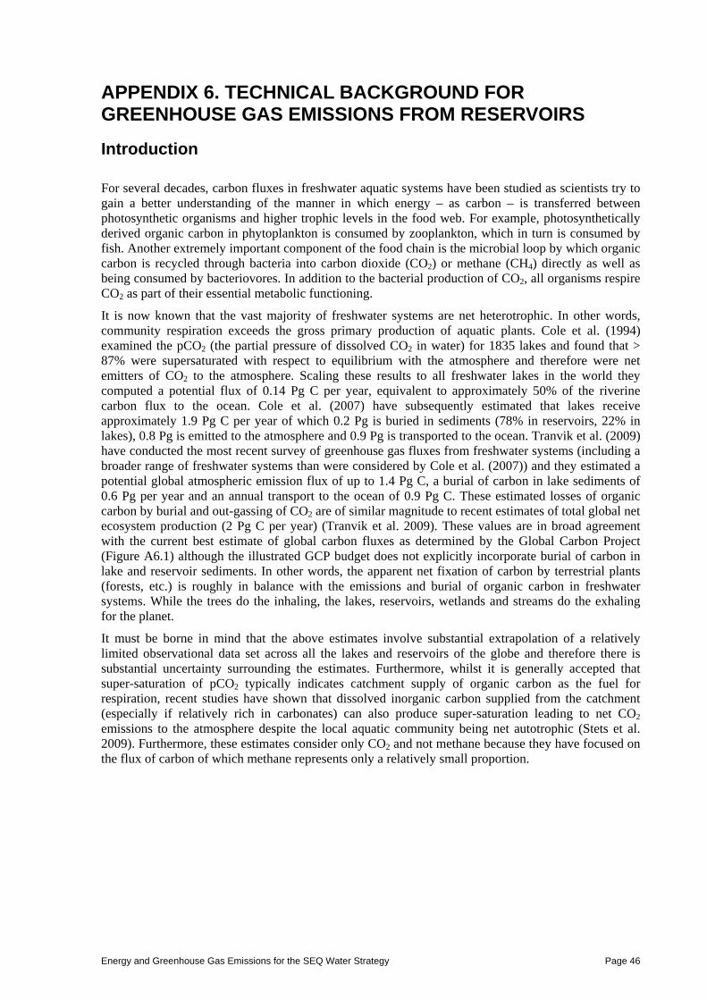
Energy and Greenhouse Gas Emissions for the SEQ Water Strategy Page 46
APPENDIX 6. TECHNICAL BACKGROUND FOR GREENHOUSE GAS EMISSIONS FROM RESERVOIRS
Introduction
For several decades, carbon fluxes in freshwater aquatic systems have been studied as scientists try to gain a better understanding of the manner in which energy – as carbon – is transferred between photosynthetic organisms and higher trophic levels in the food web. For example, photosynthetically derived organic carbon in phytoplankton is consumed by zooplankton, which in turn is consumed by fish. Another extremely important component of the food chain is the microbial loop by which organic carbon is recycled through bacteria into carbon dioxide (CO2) or methane (CH4) directly as well as being consumed by bacteriovores. In addition to the bacterial production of CO2, all organisms respire CO2 as part of their essential metabolic functioning.
It is now known that the vast majority of freshwater systems are net heterotrophic. In other words, community respiration exceeds the gross primary production of aquatic plants. Cole et al. (1994) examined the pCO2 (the partial pressure of dissolved CO2 in water) for 1835 lakes and found that > 87% were supersaturated with respect to equilibrium with the atmosphere and therefore were net emitters of CO2 to the atmosphere. Scaling these results to all freshwater lakes in the world they computed a potential flux of 0.14 Pg C per year, equivalent to approximately 50% of the riverine carbon flux to the ocean. Cole et al. (2007) have subsequently estimated that lakes receive approximately 1.9 Pg C per year of which 0.2 Pg is buried in sediments (78% in reservoirs, 22% in lakes), 0.8 Pg is emitted to the atmosphere and 0.9 Pg is transported to the ocean. Tranvik et al. (2009) have conducted the most recent survey of greenhouse gas fluxes from freshwater systems (including a broader range of freshwater systems than were considered by Cole et al. (2007)) and they estimated a potential global atmospheric emission flux of up to 1.4 Pg C, a burial of carbon in lake sediments of 0.6 Pg per year and an annual transport to the ocean of 0.9 Pg C. These estimated losses of organic carbon by burial and out-gassing of CO2 are of similar magnitude to recent estimates of total global net ecosystem production (2 Pg C per year) (Tranvik et al. 2009). These values are in broad agreement with the current best estimate of global carbon fluxes as determined by the Global Carbon Project (Figure A6.1) although the illustrated GCP budget does not explicitly incorporate burial of carbon in lake and reservoir sediments. In other words, the apparent net fixation of carbon by terrestrial plants (forests, etc.) is roughly in balance with the emissions and burial of organic carbon in freshwater systems. While the trees do the inhaling, the lakes, reservoirs, wetlands and streams do the exhaling for the planet.
It must be borne in mind that the above estimates involve substantial extrapolation of a relatively limited observational data set across all the lakes and reservoirs of the globe and therefore there is substantial uncertainty surrounding the estimates. Furthermore, whilst it is generally accepted that super-saturation of pCO2 typically indicates catchment supply of organic carbon as the fuel for respiration, recent studies have shown that dissolved inorganic carbon supplied from the catchment (especially if relatively rich in carbonates) can also produce super-saturation leading to net CO2 emissions to the atmosphere despite the local aquatic community being net autotrophic (Stets et al. 2009). Furthermore, these estimates consider only CO2 and not methane because they have focused on the flux of carbon of which methane represents only a relatively small proportion.

Energy and Greenhouse Gas Emissions for the SEQ Water Strategy Page 47
Figure A6.1: Global carbon budget as of March 2009. Figure courtesy Pep Canadel, Global Carbon Project.
Gross Versus Net Emissions – Anthropogenic Influence on Global Warming Potential
Although the gross GHG emissions from freshwater systems are clearly quite significant in comparison with terrestrial net ecosystem production and the anthropogenic change in the land-based carbon sink/source, an assessment of the anthropogenic perturbation to global warming in aquatic systems must consider the net change in GHG emissions rather than the gross emissions. If CO2 is fixed by plants, transported as dissolved organic carbon (DOC) and particulate organic carbon (POC) into aquatic systems and respired back to the atmosphere as CO2 , then there has been little, if any, consequential net change in the global warming potential due to freshwater emissions from natural lakes or constructed reservoirs. Permanent burial of organic carbon (OC) in sediments – either in lakes and reservoirs or in the ocean – could be considered long-term storage of carbon. However, burial of carbon in reservoir sediments only represents a net carbon sink from a GHG emissions perspective if the sedimenting material would not have been buried in the ocean in any event, i.e. if some proportion of the particulate carbon can reasonably be expected to be consumed and respired within the ocean.
The important additional contributions to global warming due to the presence of reservoirs arise from two factors: a one-time breakdown of soil and plant carbon as a result of inundation when a storage fills; and emission of methane rather than CO2 because conditions in reservoirs often promote anaerobic conversion of OC to CH4 rather than CO2 both in the water column and in the sediments. We are assuming that reservoir methane emissions would have occurred instead as CO2 had they been allowed to occur in a natural river channel or in the ocean.
If the presence of a reservoir results in the remineralisation as methane rather than carbon dioxide of 10% of the organic carbon load arriving from the catchment and generated internally then the global warming potential (GWP) of the emissions is increased by a factor of 2.9 assuming the remaining OC load is re-mineralised as CO2. This occurs because the global warming potential of methane is 20 times greater than that of carbon dioxide. Even if the presence of the reservoir results in the permanent burial of the remaining 90% of the OC the GWP is still doubled relative to the case of complete conversion to CO2.

Energy and Greenhouse Gas Emissions for the SEQ Water Strategy Page 48
The remainder of this review assumes that CO2 emissions from a storage (apart from those following the initial inundation) would have occurred in any event, i.e. further downstream in the river or in the ocean, had there been no reservoir to increase the time available for decomposition of organic matter and therefore CO2 emissions do not represent a substantial increase in GWP attributable to the reservoir's presence. To further simplify the analysis that follows, any burial of carbon in reservoir sediments is assumed to not represent a supplemental carbon sink but rather a relocation of an existing sink from the ocean to the reservoir.
Sources of Dissolved Carbon Dissolved inorganic and organic carbon (DIC, DOC) enters waterways through a variety of paths. Important sources of DIC in freshwater include exchange of CO2 with the atmosphere and inflow of groundwater, especially from carbonate-rich geological formations (Stets et al. 2009). Dissolved organic carbon can be supplied as exudates from primary producers, leachates of particulate organic matter, and by-products of the microbial decomposition of organic matter. It can also be supplied directly in rain (Willey et al. 2000) with continental rain having a higher concentration (~60–160 µM) compared to marine rain (~ 23 µM). A recent study of northern hemisphere systems has linked increases in stream DOC to decreases in sulphate and chloride in atmospheric fallout resulting from reductions in industrial air pollution (Monteith et al. 2007).
It seems intuitive that there should be a relationship between the land use, vegetation, climate and geology of a catchment and the concentration of DOC in waters exported from the catchment. However, it appears unlikely that a simple model relating DOC to an aggregate estimate of leaf litter will provide satisfactory accuracy as a basis for estimating GHG emissions from receiving waters.
A number of studies have been conducted that examine the leaching of carbon and nutrients from vegetation found in Australian catchments (Baldwin 1999; Howitt et al. 2008; Howitt et al. 2007; Nelson et al. 1993; Nelson et al. 1990; O'Connell et al. 2000; Qiu et al. 2005; Wallace et al. 2008; Zander et al. 2007). More than 100 DOC compounds have been observed in leachates from a floodplain river in NSW (Zander et al. 2007) and the amount of DOC per unit mass of vegetation varies significantly with the type of vegetation (Wallace et al. 2008).
Transport of DOC depends strongly on soil conditions. Nelson et al. (1993) monitored DOC in runoff from two adjacent South Australian catchments with similar climate, vegetation and land use. Concentrations of DOC differed ten-fold between these catchments (3.8 to 32 mg L-1). DOC was observed to adsorb preferentially on Cretaceous soils which have a higher clay content and specific surface area as compared to sandier Tertiary soils. Adsorption of DOC onto the clay soils did not discriminate between types of DOC. Furthermore, DOC exported from catchments does not necessarily correlate with the amount of carbon stored in the soil (Nelson et al. 1990) because more adsorptive soils (higher clay content) can have higher a soil carbon content.
Vink et al. (2007) monitored DOC fluxes from paired catchments to examine how modified land use impacted both concentration and export of DOC. Both catchments were originally native forest that was cleared over 100 years ago and used for pasture. In 1988–9 one of the catchments was converted to a pine plantation. The forested catchment had higher soil carbon (7.4%) compared to the pasture (4.8%). Although the flow-weighted mean DOC concentration was similar for both catchments (14.5 mg L-1 unimproved pasture, 15.4 mg L-1 pine forest) the pasture had much greater DOC export because the runoff yield was 3 to 5 times greater for the pasture than for the forest.
The origin of organic matter and DOC changes from terrestrial sources in headwater streams to autochthonous production in lowland areas. Vink et al. (2005) observed that the dominant supply of organic carbon in the Murrumbidgee upstream of Gundagai was supplied by terrestrial sources whereas at Darlington Pt in the much flatter reaches of the Hay Plain (~6 days travel downstream) organic carbon was supplied internally by phytoplankton growth. pCO2 decreased steadily along the river implying a decrease in CO2 flux from the river, presumably to the atmosphere as measurements of community respiration suggested loss of carbon was due to community respiration and out-gassing to the atmosphere across the air-water interface.
Once in the plains where supply of terrestrial OC is small due to limited exchange with floodplains (river regulation) and little groundwater input, the reduction in pCO2, maintenance of fairly steady

Energy and Greenhouse Gas Emissions for the SEQ Water Strategy Page 49
DOC and increasing chl (and by inference POC) requires a replacement of terrestrial OC with autochthonous OC. The decrease in pCO2 can be driven by sedimentary losses of phytoplankton through the sequestration of DIC by the algae prior to sedimentation.
Olley (2002) investigated the forms of carbon found in water, soil, leaf litter and grasses in the Murrumbidgee catchment. At the upstream end of the river, fine suspended particulate organic matter (FSPOM) was dominated by soil organic matter and C3-riparian vegetation. Further downstream the FSPOM became progressively more dominated by in-channel algal production. During flood conditions, including recession, FSPOM C was dominated by soil organic C.
The empirical evidence gathered to date suggests that a predictive model of GHG emissions from proposed reservoir developments should consider vegetation types and soil conditions in the catchment upstream of the reservoir as well as the location of the reservoir along the river (between headwaters and the ocean) in order to provide the most accurate estimate of DOC flux.
A Conceptual Model of Reservoir GHG Emissions
A basic conceptual model of the important sources, sinks and fluxes of greenhouse gases is shown in Figure A6.2. Nitrous oxide (N2O) is not considered here because its contribution from reservoirs to global warming is very small compared to carbon dioxide and methane. Much of the following description of the major GHGs is taken directly from Sherman et al. (2001).
Most Australian reservoirs more than 6 or 7 m deep are persistently thermally stratified during spring-autumn – absorption of solar radiation in the water column causes the surface waters to warm more than the deep waters. This stratification suppresses vertical transport in the water column to the extent that the interior of most reservoirs are quiescent with effective vertical diffusivities, Kz, only 10–100 times greater than molecular levels (Sherman et al. 2000). A consequence of this stratification is that dissolved oxygen becomes depleted in deeper waters (the hypolimnion) due to respiratory demands and CO2 accumulates. When dissolved oxygen is effectively exhausted (a common occurrence) then CH4 may accumulate as well (Figure A6.2).
CO2 CO2 is produced by oxidation of organic matter by bacteria, both in the water column and (predominantly) the sediments. Respiration by larger organisms is a minor source. The organic carbon is contained in living and dead phytoplankton and macrophytes (autochthonous carbon) produced within the dam, or dissolved and particulate organic material brought in by streamflow and groundwater percolation (allochthonous carbon).
Oxygen is the principal oxidant but different consortia of organic matter-consuming bacteria utilise nitrate, manganese oxides, iron oxides, and sulphate sequentially. Once all are used up, fermentation processes set in converting any remaining reactive organic matter to a mixture of CO2 and CH4. CO2 can be removed from the water by photosynthesis, by pelagic or benthic phytoplankton. Part of the organic carbon produced in situ, or entering the dam, will be buried in the sediments.
The concentration of CO2 increases with depth in the water column in the presence of stable density stratification. Density stratification is virtually always due to thermal stratification.
CH4
CH4 is produced exclusively by bacterial fermentation processes in anoxic parts of the water column and (predominantly) sediments in stratified water bodies. It is removed by methanotrophic bacteria inhabiting a narrow oxygenated zone immediately above the oxycline in stratified systems. On a molecule-for-molecule basis, CH4 has a much greater GWP than CO2, with estimates from the Intergovernmental Panel on Climate Change (IPCC) varying from 12.7 to 22.9 times the CO2 equivalent. The current value of methane for greenhouse analyses, considering a time horizon of 100 years, is accepted as 20 times the CO2 equivalent.
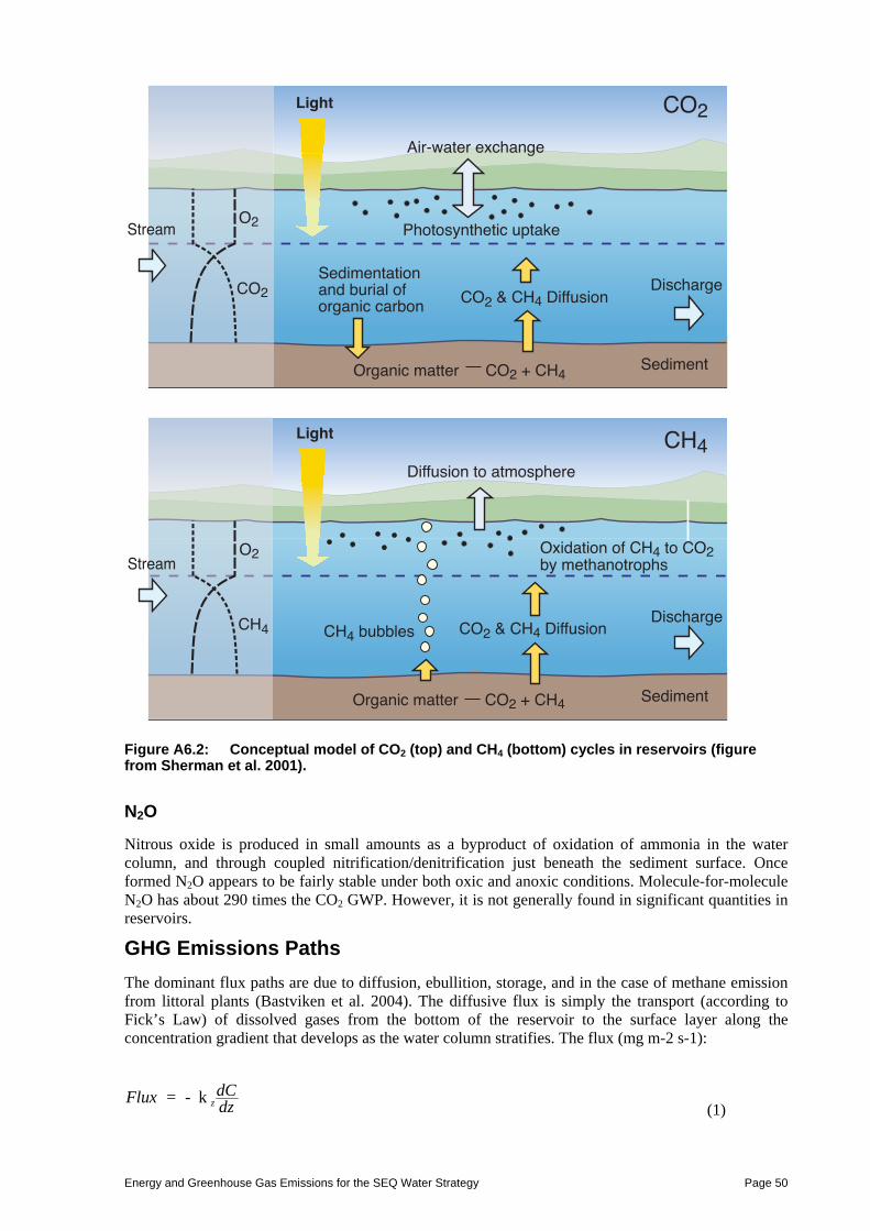
Energy and Greenhouse Gas Emissions for the SEQ Water Strategy Page 50
�����
��������
�� �������������
����������������������������������������
���������������������
��!"������#������
�
�
� ���������
���������������������$���
������
��������
�
��
����������� ����������
#����������������������������������
�����������������������
���������������������$���
�� �������������
�����
������
Figure A6.2: Conceptual model of CO2 (top) and CH4 (bottom) cycles in reservoirs (figure from Sherman et al. 2001).
N2O
Nitrous oxide is produced in small amounts as a byproduct of oxidation of ammonia in the water column, and through coupled nitrification/denitrification just beneath the sediment surface. Once formed N2O appears to be fairly stable under both oxic and anoxic conditions. Molecule-for-molecule N2O has about 290 times the CO2 GWP. However, it is not generally found in significant quantities in reservoirs.
GHG Emissions Paths
The dominant flux paths are due to diffusion, ebullition, storage, and in the case of methane emission from littoral plants (Bastviken et al. 2004). The diffusive flux is simply the transport (according to Fick’s Law) of dissolved gases from the bottom of the reservoir to the surface layer along the concentration gradient that develops as the water column stratifies. The flux (mg m-2 s-1):
Flux = - k zdCdz (1)

Energy and Greenhouse Gas Emissions for the SEQ Water Strategy Page 51
Where C is the concentration of the dissolved gas (mg m-3) z is the vertical distance (m) z is the diffusivity (m2 s-1).
Once in the surface layer, the dissolved gases will exchange with the atmosphere depending on whether the surface layer is over-saturated (flux to the atmosphere) or under-saturated (flux into the water) with respect to the concentration in the atmosphere.
Fluxair - water = k Cs - C (2)
The flux across the air-water interface, Fluxair-water, is a function of the concentration difference across the interface typically assumed as the difference between saturation Cs (equilibrium with the atmosphere) and actual concentration, C, of the dissolved gas and a wind speed-dependent gas transfer velocity1, k. There are many field and laboratory studies of gas transfer that consistently show a slow increase in the gas transfer velocity with wind speeds below 3–4 m s-1 and a much faster increase in gas transfer velocity for winds > ~4 m s-1. Estimates of GHG fluxes based on pCO2 measured in water must all include an assumption regarding the value of the gas transfer velocity.
The ebullitive flux is the flux of a gas that occurs as bubbles passing up through the water column and entering the atmosphere directly.
The storage flux refers to the fate of accumulated dissolved gases following complete mixing of the water column (which typically occurs as a result of autumnal cooling in most reservoirs). The storage flux is in addition to the flux associated with deep water discharges from dams. Many Australian dams have been constructed with only deep water outlets (Sherman 2001). When water is withdrawn directly from the hypolimnion, the high concentrations of GHGs present at depth will be rapidly out-gassed once the discharge is exposed to the atmosphere.
Finally, some forms of littoral vegetation are known to directly mediate methane emissions through the plant itself. These emissions are likely to become quantitatively more significant as the surface area of a lake decreases because the area containing vegetation occupies a greater percentage of the total water surface area. Bastviken et al. (2004) cite literature values of plant emissions in the range of 8–262 mg C m-2 d-1. In reservoirs such emissions are generally not important because of the small amount of littoral vegetation (due to erosion of top soil resulting from changing water levels) and the relatively large areas of open water.
Reservoir GHG Emission Measurement Techniques
Different methods are required to directly measure and/or calculate GHG emissions associated with the three main flux paths in reservoirs: diffusive, ebullitive and storage. Tremblay et al. (2005) provide a thorough review of the main measurement approaches.
Measurement of dissolved gas concentrations in the water column has traditionally required careful sample collection in the field followed by subsequent sample analysis using gas chromatography (GC). GC remains the gold standard for such measurements; however, a promising new approach is currently under development and testing. This new approach allows in situ measurement of dissolved gas concentration by using a pump to circulate water from the depth of interest through an equilibrator or membrane exchange module (Abril et al. 2006; Bastien et al. 2008; Frankignoulle et al. 2001). These systems allow the diffusion of the dissolved gas from the water side to come to equilibrium with the gas side. The gas side is then passed through a conventional gas analyser. Preliminary results using this technology are quite promising.
1 The gas transfer velocity is also referred to in the literature as a mass transfer coefficient and as a piston velocity.

Energy and Greenhouse Gas Emissions for the SEQ Water Strategy Page 52
Gas analysers have been used to measure CO2, CH4, and N2O where samples of gas are collected directly (rather than being dissolved in water). Non-dispersive infrared (NDIR) gas analysers have been used by Hydro Québec to measure CO2 with an accuracy of 0.2–0.5 ppm and Fourier transformed infrared (FTIR) analysers have been used to measure N2O, CH4 and CO2 concurrently with accuracies of < 20 ppm (CO2) and < 1 ppm for CH4 and N2O. A significant operational concern with the use of NDIR and FTIR gas analysers in the field is that it is essential to avoid moisture contamination of the gas entering the detectors. This requires the introduction of desiccants upstream of the instrument and careful avoidance of splashing on the boat.
Recently, a new type of gas analyser has become available that uses ‘cavity ringdown spectroscopy’ to measure CO2, CH4 and water vapour concurrently. This technology is not sensitive to water vapour contamination as it includes direct measurement of water vapour. It also provides extremely high precision (0.2 ppm CO2, 0.001 ppm CH4).
Diffusive Flux
The diffusive flux is often estimated using measurements of pCO2 in the surface layer and applying equation (2). This involves making some (possibly heroic) assumptions regarding the gas transfer velocity (i.e. if wind data are not available).
Ebullitive Flux
A commonly employed approach by Hydro Québec and other investigators is direct measurement using floating chambers deployed on the surface of the water. Chamber measurements include both diffusive and ebullitive fluxes. These chambers provide a gas tight seal with the water and employ a recirculating gas line through which the head space gas is circulated through a gas analyser. About 10–30 minutes is required for a flux measurement.
Chambers may also be deployed submerged below the water surface in which case they measure just the ebullitive flux.
Storage
The mass of a dissolved gas present in a reservoir, MC, is easily computed by measuring the vertical concentration profile of a gas in the water column, C(z) and then integrating over the depth of the reservoir, H,
M C = C z A z dz0
H
(3) During the stratified period, methane accumulates in the hypolimnion. Despite a strong diffusive flux along the concentration gradient, there is seldom any appreciable methane detected in the surface layer of lakes and reservoirs because methanotrophic bacteria, typically located at the boundary between oxic and hypoxic waters, oxidise the methane before it can enter the surface layer (Schubert et al. 2006). This explains why diffusive fluxes of methane are negligible compared to the ebullitive flux which cannot be effectively consumed by methanotrophs.
The storage flux can be computed by differencing the mass of methane in the water column just prior to and just after seasonal overturn of the water column. This calculation assumes that the difference in mass of methane is entirely out-gassed whereas it might be the case that some fraction of the stored methane is oxidised by bacteria during the period of overturn.
It is not known what impact the overturning process exerts on the ability of methanotrophs to consume methane. During overturn, the surface-mixed layer deepens progressively over the course of 1–3 weeks (typically). As the mixed layer deepens it entrains fluid from the top of the thermocline (and chemocline). This process will disperse the bacteria throughout the surface layer, prevent their

Energy and Greenhouse Gas Emissions for the SEQ Water Strategy Page 53
accumulation at the top of the chemocline, and weaken the methane concentration gradient adjacent to their cell walls. All of these factors are expected to radically diminish the capacity of the methanotrophic community to oxidise the methane being entrained into the surface layer. This would make an excellent PhD thesis topic.
The storage flux has not received much attention apart from Huttunen et al.’s (2003) measurement of CH4 accumulated during winter in an ice-covered lake and subsequently released during the spring thaw. They used chambers to measure emission and estimated that this loss of winter-stored methane could contribute 22–48% of the total methane emission from the lake.
Another measurement approaching an estimate of storage flux was made by Sherman et al. (2001) in Chaffey Dam who computed the loss of methane that occurred over a seven-day period during which a bubble plume destratifier was operated. In physical terms, this process differs from seasonal overturn because it carries deep water to the surface over a relatively small area as opposed to a uniform deepening of the surface layer across the entire reservoir.
Reservoir GHG Emissions
Virtually all reservoir GHG emission studies have been conducted in North America, Europe and Brazil and by far the most detailed studies relate to boreal and tropical systems. A paucity of information regarding temperate climate storages was highlighted by the World Commission on Dams (WCD 2000) and this situation has changed little since the WCD report was released. The Asia-Pacific region, which has over 60% of the world’s large dams, has virtually no studies of emissions apart from recent measurements undertaken in Tasmania and in some of the Snowy Hydro reservoirs plus a few data points from Dartmouth and Chaffey Dams as reported by Sherman et al. (2001) and recent measurements undertaken by Grinham (pers. comm. 2009) at three storages in SEQ. GHG Emissions Following Inundation
When a reservoir is first inundated following construction there will be a period of elevated emissions which decreases asymptotically over ~10 years to a quasi-steady value which continues indefinitely into the future and reflects the supply of allochthonous carbon (both DIC and DOC) from the catchment (Tremblay et al. 2005). Direct measurements of emissions following inundation have been conducted mainly in boreal forested catchments of Canada and Scandinavia and in tropical storages in Brazil. Rosa et al.(1997a) measured emissions from two Brazilian reservoirs and found that herbaceous plants decomposed 50% within 2 weeks and 70–90% in 4 months. Because woody matter (twigs, branches, stems) decays more slowly than leaf material, the authors recommend an average decomposition rate of 40% over 4 months. They warn, however, that the actual decomposition rates for inundated biomass are highly variable and decrease under anaerobic conditions. Methane emissions from inundated marshes, flatlands and lakes in these storages ranged from 11–189 mg CH4 m
-2 d-1.

Energy and Greenhouse Gas Emissions for the SEQ Water Strategy Page 54
Figure A6.3: Change in reservoir GHG emissions over time. Data courtesy L. Gagnon, pers. comm. 2001.
Measured emissions for a number of Hydro Québec reservoirs are compared to emissions from natural lakes in Figure A6.3. These data show the decrease over time to a quasi-steady value after ~10 years and they also show that the quasi-steady emissions fall within the range observed in natural lakes in similar climatic conditions. The implication here is that after the period of initial release of inundated carbon, a reservoir emits GHGs in a similar way to natural lakes, i.e. the same underlying processes are occurring in both constructed and natural water bodies. Emissions from these boreal systems occur overwhelmingly as CO2. Methane Emissions from Aquatic Systems
Bastviken et al. (2004) reported methane emissions made in 73 mostly small (< 100 ha) lakes in the northern hemisphere and found that the ebullitive (bubble) flux was 50% of the total flux, the diffusive and storage flux (through water column overturn and release through turbines) ranged from 0–50% with the storage flux becoming relatively more important in lakes with anoxic zones. Ebullition was observed in 60–80% of water columns < 2 m deep; a water column depth of 0.5–1 m had the highest occurrence of ebullition. The diffusive flux was observed to depend on latitutude with higher fluxes observed in warmer climes. Considering all the lakes reported by Bastviken et al. (2004) the mean and median daily methane emission rates were 26 and 6.8 mg-C m-2 d-1, of which 70% was ebullition flux, 12% diffusion flux and 19% storage flux. Kelly and Chynoweth (1981) found that methane fluxes from surficial sediments in several lakes was linearly related to the supply of organic matter and that the organic matter was converted to methane at close to the maximum theoretical value of ~40%. They observed also an (expected) exponential temperature dependence of methane release on their sediment core incubations with a Q10 of 2.4 ± 1.1. When comparing sediment CH4 fluxes as a function of hypolimnion temperature from different lakes, a 10°C increase in temperature corresponded to a 10-fold increase in CH4 flux and they suggest that

Energy and Greenhouse Gas Emissions for the SEQ Water Strategy Page 55
the role of temperature impacts both the flux of organic matter through water column stratification as well as the microbial reaction that converts the organic matter flux into methane. Huttunen et al. (2002) used static chambers to measure CH4 emissions from two Finnish hydropower reservoirs and observed fluxes ranging from -0.4–244 mg m-2 d-1 with mean fluxes of 12.4 and 33.3 mg m-2 d-1 in Lokka Reservoir during 1994 and 1995, respectively and a flux of 3.5 mg m-2 d-1 in Porttipahta in 1995. Bubble gas composition varied between reservoirs and contained 70–80% methane in Lokka but < 35% methane in Porttipahta. In another study, Huttunen et al. (2001a) examined the impact of artificial oxygenation on the global warming potential of CH4, CO2 and N2O release during ice-out in two pairs of small ice-covered lakes. Introduction of oxygen was found to suppress methane production dramatically (a 50–100 fold reduction in GWP) whereas there was negligible impact on CO2 emissions. The global warming contribution of nitrous oxide emissions was << 1% in natural lakes and < 4% in oxygenated lakes. In tropical climates, reservoir methane emission is much higher than is observed in the colder boreal regions. Galy-Lacaux et al. (1999) also measured the spatial variability of the ebullitive flux and found much higher emissions in shallow regions. They also found emissions dropped substantially between the first and fourth year following inundation of the reservoir (Table A6.1).
Table A6.1: Methane ebullition flux in Petit Saut Reservoir as a function of water column depth during the first year (1994) and fourth year (1997) following inundation (data from Galy-Lacaux et al. 1999).
Ebullition of CH4 mg m-2 d-1 (std dev) Depth range (m)
1994 1997
0–3 1400 (650, n = 10) 164 (55, n = 50)
4–6 770 (300, n = 10) 66 (10, n = 36)
7–9 240 (90, n = 5) 55 (1, n = 32)
> 10 0 (n = 10) 0 (n = 16)
Temporal Changes in GHG Emissions
Several authors have reported pronounced temporal variability in methane emissions on both seasonal and diurnal time scales. Abril et al. (2006) made continuous measurements of pCO2 and pCH4 in surface waters and found that pCH4 varied from < 50 to > 400 µatm over as little as 8 hours and that this variability corresponded to wind mixing events that were believed to have entrained methane-rich water from below the surface-mixed layer. Rosa et al. (1997b) reported roughly a three-fold variation in fluxes depending on the duration of the measurement and the time of day. Large seasonal variability in ebullition is frequently observed (e.g. Huttunen et al. 2001b) as methane production rates respond to seasonal changes in hypolimnetic temperature (Kelly and Chynoweth 1981). Australian Reservoir GHG Emissions
The first report of GHG emissions from an Australian reservoir was by Sherman et al. (2001) who estimated emissions from a single profile at Dartmouth Dam and from a longer data set at Chaffey Dam. Based on a single profile (the only measurement available) they found the surface layer pCO2 was ~8 times greater than saturation and estimated the diffusive flux as 21–168 mg CO2 m
-2 d-1. At depth (below 80 m) the concentration of CO2 was approximately 7 times greater and because only deep water can be released the turbine flux was estimated to be 530 mg CO2 m
-2 d-1. Dartmouth Dam had negligibly small methane concentrations throughout the water column. At Chaffey Dam, Sherman et al. (2001) computed a storage flux (actually a loss due to operation of a bubble-plume destratifier over 3 days) loss of methane of 43 tonnes over one week. This equates to an annual daily flux of ~24 mg CH4 m-2 d-1. The methane concentration gradient was estimated to produce a flux from the hypolimnion to the base of the surface layer of 220–1760 mg CH4 m
-2 d-1, all of which was assumed to be oxidised by methanotrophic bacteria as there was no appreciable
Energy and Greenhouse Gas Emissions for the SEQ Water Strategy Page 56
concentration measured in the surface layer. Over 18 months of record, the surface layer of Chaffey Dam was always supersaturated with CO2 compared to atmospheric equilibrium with concentrations varying from ~2 to 12 mg CO2 L
-1. Measurements made by Hydro Québec in a range of reservoirs operated by Hydro Tasmania and Snowy Hydro showed these storages to be relatively low emitters compared to other storages in the world (Tremblay, pers. comm. 2008). This low emission probably reflects the relatively pristine, nutrient poor nature of the catchments and the relatively cold climates (no specific flux values are currently available.) Grinham (pers. comm. 2008, 2009) has provided data regarding methane fluxes measured using chambers at Wivenhoe, Little Nerang and Borumba Dams. Figure A6.4 shows high spatial (and possibly temporal) variability in emissions from Wivenhoe Dam. The existing reservoir methane emission data is shown for Australian storages in Table A6.2 and for reservoirs and lakes in boreal and tropical climates in Table A6.3. Insufficient measurements have been made to accurately assess seasonal variability in emissions within a reservoir.
Figure A6.4: Methane emissions from Wivenhoe Dam. Figure courtesy A. Grinham, University of Queensland.

Energy and Greenhouse Gas Emissions for the SEQ Water Strategy Page 57
Table A6.2: Measured methane emissions from Australian reservoirs.
CH4 mg m2 d-1 Notes Location
low med high Wivenhoe (n > 8) 24 40 73 chamber data from Grinham
Borumba (n = 1) 80 chamber data from Grinham
Little Nerang (n = 3) 1,000 chamber data from Grinham
Chaffey Dam (n = 2) 38 220 1760 profile data, flux-gradient from Sherman et al. (2001)
Table A6.3: Methane fluxes from reservoirs and lakes in boreal and tropical climates.
CH4 mg m2 d-1 Notes Location
mean median low high 73 mostly small (< 100 ha) northern hemisphere lakes
26 6.8 0.03 162 Bastviken et al. (2004)
2 pairs of shallow ice-covered Finnish lakes. One pair oxygenated, one pair natural
241 3.3 (oxy) as CO2-e
(Huttunen et al. 2001b)
Lokka Reservoir 9.3 (1994) 25 (1995)
16 (1994) 12 (1995)
-0.4 -6.5
48 244
(Huttunen et al. 2002)
Porttipahta 2.6 3 -0.5 7.6 (Huttunen et al. 2002)
Petit Saut 260 (Galy-Lacaux et al. 1999) Tucurui 67 ± 45 (Lima and Novo 1999)

Energy and Greenhouse Gas Emissions for the SEQ Water Strategy Page 58
Reservoir Methane References ABRIL, G., S. RICHARD and F. GUÉRIN. 2006. In situ measurements of dissolved gases (CO2 and CH4)
in a wide range of concentrations in a tropical reservoir using an equilibrator. Science of the Total Environment 354: 246–51.
BALDWIN, D.S. 1999. Dissolved organic matter and phosphorus leached from fresh and 'terrestrially' aged river red gum leaves: implications for assessing river-floodplain interactions. Freshwater Biology 41: 675–85.
BASTIEN, J., J.-L. FRÉCHETTE and R. H. HESSLEIN. 2008. Continuous Greenhouse Gas Monitoring System – Operating Manual. Manitoba Hydro Department of Fisheries and Oceans Canada, Hydro-Québec.
BASTVIKEN, D., J. COLE, M. PACE and L. TRANVIK. 2004. Methane emissions from lakes: Dependence of lake characteristics, two regional assessments, and a global estimate. Global Biogeochemical Cycles 18: GB4009.
COLE, J. J., N. F. CARACO, G. W. KLING and T. K. KRATZ. 1994. Carbon dioxide supersaturation in the surface waters of lakes. Science 265: 1568–70.
COLE, J. J. and others. 2007. Plumbing the global carbon cycle: Integrating inland waters into the terrestrial carbon budget. Ecosystems 10: 171–84.
FLANAGAN, K. M., E. MCCAULEY and F. WRONA. 2006. Freshwater food webs control carbon dioxide saturation through sedimentation. Global Change Biology 12: 644–651.
FRANKIGNOULLE, M., A. BORGES and R. BIONDO. 2001. A new design of equilibrator to monitor carbon dioxide in highly dynamic and turbid environments. Water Research 35: 1344–47.
GALY-LACAUX, C., R. DELMAS, G. KOUADIO, S. RICHARD and P. GOSSE. 1999. Long-Term Greenhouse Gas Emissions From Hydroelectric Reservoirs in Tropical Forest Regions. Global Biogeochem. Cycles 13(2): 503–517.
HOWITT, J. A., D. S. BALDWIN, G. N. REES and B. T. HART. 2008. Photodegradation, interaction with iron oxides and bioavailability of dissolved organic matter from forested floodplain sources. Marine and Freshwater Research 59: 780–91.
HOWITT, J. A., D. S. BALDWIN, G. N. REES and J. L. WILLIAMS. 2007. Modelling blackwater: Predicting water quality during flooding of lowland river forests. Ecological Modelling 203: 229–42.
HUTTUNEN, J. T., J. ALM, E. SAARIJÄRVI, K. MATTI LAPPALAINEN, J. SILVOLA and P. J. MARTIKAINEN. 2003. Contribution of winter to the annual CH4 emission from a eutrophied boreal lake. Chemosphere 50: 247–50.
HUTTUNEN, J. T., T. HAMMAR, J. ALM, J. SILVOLA and P. J. MARTIKAINEN. 2001a. Greenhouse Gases in Non-Oxygenated and Artificially Oxygenated Eutrophied Lakes during Winter Stratification. Journal of Environmental Quality 30: 387–94.
HUTTUNEN, J. T., K. M. LAPPALAINEN, E. SAARIJÄRVI, T. VÄISÄNEN and P. J. MARTIKAINEN. 2001b. A novel sediment gas sampler and a subsurface gas collector used for measurement of the ebullition of methane and carbon dioxide from a eutrophied lake. The Science of the Total Environment 266: 153–58.
HUTTUNEN, J. T. and others. 2002. Fluxes of CH4, CO2, and N2O in hydroelectric reservoirs Lokka and Porttipahta in the northern boreal zone in Finland. Global Biogeochem. Cycles 16(1): 1003.
KELLY, C. A. and D. P. CHYNOWETH. 1981. The Contributions of Temperature and of the Input of Organic-matter in Controlling Rates of Sediment Methanogenesis. Limnology and Oceanography 26: 891–97.
LIMA, I. B. T. and E. M. M. L. NOVO. 1999. Carbon flows in the Tucuruí reservoir. p. 78–84. In Rosa, L. P., AND M. A. dos Santos [eds.] Dams and Climate Change. COPPE.
MONTEITH, D. T. and others. 2007. Dissolved organic carbon trends resulting from changes in atmospheric deposition chemistry. Nature 450: 537–41.
NELSON, P. N., J. A. BALDOCK and J. M. OADES. 1993. Concentration and Composition of Dissolved Organic-carbon in Streams in Relation to Catchment Soil Properties. Biogeochemistry 19: 27–50.
NELSON, P. N., E. COTSARIS, J. M. OADES and D. B. BURSILL. 1990. Influence of Soil Clay Content on Dissolved Organic-matter in Stream Waters. Australian Journal of Marine and Freshwater Research 41: 761–74.
O'CONNELL, M., D. S. BALDWIN, A. I. ROBERTSON and G. REES. 2000. Release and bioavailability of dissolved organic matter from floodplain litter: influence of origin and oxygen levels. Freshwater Biology 45: 333–42.
OLLEY, J. M. 2002. Organic carbon supply to a large lowland river and implications for aquatic ecosystems. p. 27–33. In Dyer, F. J., M. C. Thoms, AND J. M. Olley [eds.] The Structure, Function

Energy and Greenhouse Gas Emissions for the SEQ Water Strategy Page 59
and Management Implications of Fluvial Sedimentary Systems. Proceedings of an International Symposium Held at Alice Springs, Australia. IAHS.
QIU, S., A. J. MCCOMB, R. W. BELL and J. A. DAVIS. 2005. Estimating production of gilvin from catchment leaf litter during seasonal rains. Marine and Freshwater Research 56: 843–49.
ROSA, L. P., S. DOS, MARCO AURÉLIO, J. G. TUNDISI and B. M. SIKAR. 1997a. Measurements of greenhouse gas emissions in Samuel, Tucuruí and Balbina dams - Brazil. p. 41–55. In Rosa, L. P., AND M. A. dos Santos [eds.] Hydropower Plants and Greenhouse Gas Emissions. COPPE.
ROSA, L. P., B. M. SIKAR, E. M. SIKAR and S. DOS, MARCO AURÉLIO. 1997b. A model for CH4 and CO2 emission mean life in reservoir based on data from an Amazonian hydroplant. p. 102–11. In Rosa, L. P., AND M. A. dos Santos [eds.] Hydropower Plants and Greenhouse Gas Emissions. COPPE.
SCHUBERT, C. J. and others. 2006. Aerobic and anaerobic methanotrophs in the Black Sea water column. Environmental Microbiology 8: 1844–56.
SHERMAN, B. S. 2001. Scoping options for mitigating cold water discharges from dams. p. 12–28. In Phillips, B. [ed.] Thermal pollution of the Murray-Darling Basin waterways: Workshop held at Lake Hume 18-19 June 2001: Statement and recommendations plus supporting papers. Inland Rivers Network, World Wide Fund for Nature Australia.
SHERMAN, B. S., P. FORD, A. MITCHELL and G. HANCOCK. 2001. Greenhouse gas emissions from reservoirs - is Australian hydropower environmentally friendly? p. 1–10. In Grimston, J. [ed.] Proc. NZSOLD/ANCOLD 2001 Conference on Dams: Dams – Development, Sustainability and Performance. ANCOLD.
SHERMAN, B. S., J. WHITTINGTON and R. L. OLIVER. 2000. The impact of artificial destratification on water quality in Chaffey Reservoir. Arch. Hydrobiol. Spec. Issues Advanc. Limnol. Limnology and Lake Management 2000+ 55: 15–29.
STETS, E. G., R. G. STRIEGL, G. R. AIKEN, D. O. ROSENBERRY and T. C. WINTER. 2009. Hydrologic support of carbon dioxide flux revealed by whole-lake carbon budgets. Journal of Geophysical Research-biogeosciences 114: G01008.
TRANVIK, L. J. and others. 2009. Lakes and Impoundments as Regulators of Carbon Cycling and Climate. Limnol. Oceanogr. submitted:
TREMBLAY, A., L. VARFALVY, G. ROEHM and M. GARNEAU. 2005. Greenhouse Gas Emissions - Fluxes and Processes. Springer.
VINK, S., P. W. FORD, M. BORMANS, C. KELLY and C. TURLEY. 2007. Contrasting nutrient exports from a forested and an agricultural catchment in south-eastern Australia. Kluwer Academic Publishers.
VINK, S., M. BORMANS, P. W. FORD and N. J. GRIGG. 2005. Quantifying ecosystem metabolism in the middle reaches of Murrumbidgee River during irrigation flow releases. Mar. Freshwater Res. 56: 227–41.
WALLACE, T. A., G. G. GANF and J. D. BROOKES. 2008. A comparison of phosphorus and DOC leachates from different types of leaf litter in an urban environment. Freshwater Biology 53: 1902–13.
WCD, S. 2000. Dams and Global Climate Change, Thematic Review II.2 prepared as an input to the World Commission on Dams. World Commission on Dams.
WILLEY, J. D., R. J. KIEBER, M. S. EYMAN, J. AVERY and G. BROOKS. 2000. Rainwater Dissolved Organic Carbon: Concentrations and Global Flux. Global Biogeochemical Cycles 14(1): 139–148.
ZANDER, A., A. G. BISHOP, P. D. PRENZLER and D. S. RYDER. 2007. Allochthonous DOC in floodplain rivers: Identifying sources using solid phase microextraction with gas chromatography. Aquatic Sciences 69: 472–83.

Energy and Greenhouse Gas Emissions for the SEQ Water Strategy Page 60
APPENDIX 7. CENTRALISED WASTEWATER DIFFUSE GREENHOUSE GAS EMISSIONS
The following tables are reproduced from work published by d(De Haas et al., 2009) and describe the data used in this report. Table A7.1 provides the assumptions for emission factors and greenhouse gas calculations. Table A7.2 provides a description of the wastewater treatment by plant types in SEQ. Note that ten plants account for about three-quarters of average dry weather flow (ADWF) in the sample of 35 plants in SEQ. The sample itself captures most plants in SEQ, excluding only four plants. Table A7.3 provides a breakdown of GHG emissions by plant type and shows the emissions from diffuse nitrous oxide and methane emissions as well as emissions from other sources such as energy. Diffuse nitrous oxide and methane emissions were approximately one-third of emissions for most plant types except plant Type 1+ Cogen where they are approximately two-thirds. However, there is very large uncertainty associated with the emission factors for diffuse nitrous oxide and methane emissions. Table A7.1: Emission factors and assumptions for greenhouse gas emissions for SEQ wastewater treatment plants (De Haas et al., 2009).
(continued over page)

Energy and Greenhouse Gas Emissions for the SEQ Water Strategy Page 61

Energy and Greenhouse Gas Emissions for the SEQ Water Strategy Page 62
Table A7.2: Wastewater treatment plant size and type in SEQ survey (De Haas et al., 2009).

Energy and Greenhouse Gas Emissions for the SEQ Water Strategy Page 63
Table A7.3: Greenhouse gas results for four typical plant types in SEQ (De Haas et al., 2009).

Energy and Greenhouse Gas Emissions for the SEQ Water Strategy Page 64
APPENDIX 8. ON-SITE WASTEWATER DIFFUSE GHG EMISSIONS
The following Tier 1 estimate applies default values for the emission factor and activity parameters from ‘Chapter 6 – Wastewater Treatment and Discharge’ of the ‘2006 IPCC Guidelines for National Greenhouse Gas Inventories’ (referred to as the IPCC Guidelines in this section). This method is considered ‘good practice’ for countries with limited data. Sludge removal and recovery of methane are assumed to be the default zero values (IPCC 2006, p6.9). As a result, Equation 6.1 from the IPCC Guidelines was reduced to:
CH4 emissions = EFseptic tank * TOWseptic
Where: CH4 emission is the kg CH4/yr EFseptic tank is the septic tank emission factor TOWseptic is the total organics in the wastewater entering the septic tank, kg BOD/yr
The emission factor (EF) for septic tanks was developed using Equation 6.2 from the IPCC Guidelines:
EFseptic = Bo • MCF
Where: EFseptic is the septic tank emission factor, kg CH4/kg BOD Bo is the maximum CH4 producing capacity, kg CH4/kg BOD MCF is the methane correction factor (fraction)
A default Bo of 0.6 kg CH4/kg BOD or 0.25 kg CH4/kg COD was assumed based upon Table 6.2 (of the IPCC Guidelines) ‘Default Maximum CH4 Producing Capacity (Bo) For Domestic Wastewater’. An MCF of 0.5 was assumed for septic tanks following Table 6.3 (of the IPCC Guidelines) which notes that ‘half of BOD settles in anaerobic tank’. This gives an EF of 0.3 kg CH4/kg BOD or 0.12 kg CH4/kg COD. Note that these values were based upon expert judgement of the lead authors of the IPCC Guidelines. The Total Organics in the Wastewater (TOW) was estimated using equation 6.3 of the IPCC Guidelines. The equation was simplified as there was no industrial discharge to increase the BOD loading.
TOWseptic tank = P * BOD * 0.001 *365 Where:
TOWseptic tank is the total organics in the septic tank wastewater kg BOD/yr P is the population each year BOD is the country-specific BOD, g/person/day
The BOD was assumed to be 65 g/person/day based upon the Water Services of Australia publication ‘Affordable Water Supply and Sewerage for small communities’ which gave an estimate of 60–70 g BOD per person per day. (WSAA, 1999). This value is within the range of a number of regions reported in Table 6.4 of the IPCC Guidelines such as ‘Canada, Europe, Russia, Oceania’ as well as the USA. However, the range of values for the USA is large (50–120 g/person/day) and there are a number of other countries with lower BOD values. Population was estimated from the number of tanks and assumed 2.4 people per household. Only on-site systems with anaerobic processes were considered. The estimate of on-site anaerobic systems was based upon a review of on-site systems in SEQ (Beal et al., 2003). As noted in 4.6 Energy Use for On-Site Wastewater Systems it was estimated that in 2003 there were 127,000 on-site wastewater systems in SEQ. Substituting these values into equation 6.3 gives a TOW of 7 200,000 kg BOD/year in 2003 (127,000 tanks* 2.4 people/tank * 65 g BOD/person/day * 0.001 g/kg * 365 days/year). Substituting this TOW into equation 6.1 gives 2 200,000 kg CH4/year (7 200,000 *0.3). This is equal to 54,000 tonnes CO2-e/year in 2003 and similar calculations can be performed for 2013 and 2056 to provide a long-term approximation of on-site methane emissions.

Urban Water Security Research Alliance
www.urbanwateralliance.org.au