energetically consistent boundary conditions for electromechanical

International Journal of Solids and Structures 41 (2004) 6291–6315

www.elsevier.com/locate/ijsolstr

Energetically consistent boundary conditionsfor electromechanical fracture

Chad M. Landis *

Department of Mechanical Engineering and Materials Science, MS 321, Rice University, P.O. Box 1892, Houston, TX 77251-1892, USA

Received 9 December 2003; received in revised form 25 May 2004

Available online 2 July 2004

Abstract

Energetically consistent crack face boundary conditions are formulated for cracks in electromechanical materials.

The model assumes that the energy of the solid can be computed from standard infinitesimal deformation theory and

that the opening of the crack faces creates a capacitive gap that can store electrical energy. The general derivation of

the crack face boundary conditions is carried out for non-linear but reversible constitutive behavior of both the solid

material and the space filling the gap. It is shown that a simple augmentation of the J-integral can be used to

determine the energy release rate for crack advance with these boundary conditions. The energetically consistent

boundary conditions are then applied to the Griffith crack problem in a polar linear piezoelectric solid and used to

demonstrate that the energy release rate computed near the crack tip is equivalent to the total energy release rate for

the solid-gap system as computed from global energy changes. A non-linear constitutive law is postulated for the crack

gap as a model for electrical discharge and the effects of the breakdown field on the energy release rate are ascer-

tained.

� 2004 Elsevier Ltd. All rights reserved.

Keywords: Piezoelectricity; Polarized material; Electrical discharge; Griffith crack; Boundary conditions; Energy release rates

1. Introduction

A significant body of work has appeared in the last few decades on the fracture mechanics of linear

piezoelectric materials. Thorough reviews of the literature can be found in McMeeking (1999), Zhang et al.

(2001) and Chen and Lu (2002). A point of contention among differing modeling approaches is the crack

face boundary condition for the so-called ‘‘insulating’’ crack problem. Herein, three approaches have re-

ceived considerable attention, (1) the impermeable crack model, (2) the permeable or ‘‘closed’’ crack model,

* Corresponding author. Tel.: +1-713-348-3609; fax: +1-713-348-5423.

E-mail address: [email protected] (C.M. Landis).

0020-7683/$ - see front matter � 2004 Elsevier Ltd. All rights reserved.

doi:10.1016/j.ijsolstr.2004.05.062

mail to: [email protected]

6292 C.M. Landis / International Journal of Solids and Structures 41 (2004) 6291–6315

and (3) the ‘‘exact’’ boundary conditions. When a cracked body is subjected to certain combinations of

mechanical and electrical loads the crack faces will open and usually some type of fluid (usually air) will fill

the void. Since the dielectric permittivity of air is much smaller than that of most piezoelectric ceramics of

technological interest, the impermeable crack model approximates the permittivity of the gap as zero. Thisimplies that the crack gap does not support any electric displacement, and continuity of electric dis-

placement at the crack surfaces implies that the normal component of electric displacement on the crack

surfaces must vanish. In contrast, the permeable crack model assumes that the crack does not perturb the

electrical fields directly and that both the electric potential and the normal component of electric dis-

placement are continuous across the crack faces. In this sense, the crack is treated as if it remains closed in

its undeformed configuration. Finally, the ‘‘exact’’ electrical boundary conditions originally proposed by

Hao and Shen (1994) attempt to account for the fact that the permittivity of the crack gap is in fact finite

and the crack can in fact be open. Hence, the electric field in the gap is approximated as the potential dropdivided by the crack opening displacement and the electric displacement in the gap is just this electric field

multiplied by the dielectric permittivity of the gap material. Each of the model types described assumes that

the crack faces are traction free.

Simply by considering the discussion of these three models for the boundary conditions it is clear that

the ‘‘exact’’ electrical boundary conditions are the most physically realistic. However, recently

McMeeking (2004) investigated the energy release rates for a Griffith crack using this type of crack face

boundary condition and found that there exists a discrepancy between the energy release rate as com-

puted from energy changes of the entire system, i.e. the total energy release rate, and the crack tip energyrelease rate. Here it is worthwhile to discuss why such a discrepancy between the total and crack tip

energy release rates is problematic for the system under consideration. First, all parts of the system are

assumed to be conservative, i.e. there is no dissipation except for energy flux through the crack tip.

Second, the crack tip is assumed to be able to sustain a singularity in the electromechanical fields and no

model is used to represent the material separation process ahead of the crack. This is in contrast to

growing cracks in dissipative materials or models for material separation like the Dugdale–Barenblatt

model, wherein distinct far field or applied energy release rates (not equivalent to the total energy release

rate) and local crack tip energy release rates are commonly identified. In an entirely conservative systemthe crack tip energy release rate can be computed either from a crack closure integral or from the J -integral with a small contour near the crack tip. Such a calculation yields the amount of energy

‘‘flowing’’ into the crack tip for an infinitesimal amount of crack advance. Next, the total energy release

rate for a conservative system is calculated by assembling the stored energy of all parts of the material

system, including any parts of the crack gap that can store energy, and the potential energy of the

loading system and then differentiating this energy with respect to crack length (care must be taken in the

interpretation of this result when there are two crack tips). Note again that the definition of the total

energy release rate used here for conservative systems is not the same as the far field or applied energyrelease rate that is used when dissipation is modeled directly during crack growth. Therefore, since all

sources of energy are accounted for when computing the total energy release rate, including the energy

entering the crack gap, and since there are no other dissipative sinks for energy to flow to aside from the

crack tip, the total energy release rate must be equal to the energy release rate computed at the crack tip

within a physically consistent model for the system. Hence, a discrepancy between the total and crack tip

energy release rates in a conservative system is unsettling and casts doubt on the validity of the ‘‘exact’’

electrical boundary conditions.

In this work energetically consistent boundary conditions will be derived with an electrical componentthat is identical to the ‘‘exact’’ electrical boundary condition plus an additional closing traction. The model

Griffith crack system will be used to demonstrate that these boundary conditions make the electrical en-

thalpy of the piezoelectric solid/crack void system stationary and that the total energy release rate is in fact

equivalent to the crack tip energy release rate.

C.M. Landis / International Journal of Solids and Structures 41 (2004) 6291–6315 6293

2. Theoretical foundations

Consider the electromechanically active solid depicted in Fig. 1. The equations governing a small

deformation, quasi-static, isothermal boundary value problem for the solid are as follows. Mechanicalequilibrium governs the stress distributions as

Fig. 1.

the dir

tractio

rji;j þ bi ¼ 0 and rji ¼ rij in V ð2:1Þ

ðrþji � r�

ji Þnj ¼ ti on S ð2:2Þ

Here rij represents the Cartesian components of the Cauchy stress tensor, bi the components of the body

force per unit volume, ti the components of the surface traction, and ni the components of the unit normal

to the surface pointing from the + side to the ) side as illustrated in Fig. 1. In all cases summation isassumed from 1 to 3 over repeated indices, and the notation ; j represents partial differentiation with respect

to xj, i.e. ;j � o=oxj. Note that Eq. (2.1) neglects any electrical ‘‘Maxwell stress’’ terms that could potentially

give rise to a body force due to electrical effects.

Next, the components of the infinitesimal strain tensor eij are related to the components of the material

displacement ui as

eij ¼1

2ðui;j þ uj;iÞ ð2:3Þ

Under quasi-static conditions, the electrical field variables are governed by Gauss’ law and Maxwell’s law

that states that the electrical field must be irrotational.

Di;i ¼ q in V ð2:4Þ

ðDþi � D�

i Þni ¼ �x on S ð2:5Þ

Ei ¼ �/;i ð2:6Þ

An electromechanically active solid of volume V bounded by the surface S. The ‘‘+’’ and ‘‘)’’ sides of the surface are related to

ection of the unit normal to the surface n as shown. The applied electromechanical loadings include specified mechanical surface

ns t and body forces b, and electrical surface free charge densities x and body free charge densities q.


Here, Di are the components of the electric displacement, q is a body charge per unit volume, x is a surface

charge per unit area, Ei are the components of the electric field, and / is the electric potential.

To complete the set of equations the constitutive law for the material is required. In this work only

conservative materials will be considered. Hence, an electrical enthalpy density h, Li and Ting (1957), canbe defined such that

h ¼ ~u� EiDi ð2:7Þ

where ~u is the internal energy density of the material. For conservative materials

d~u ¼ rijdeij þ EidDi ð2:8Þ

Then, Eq. (2.8) implies that

dh ¼ rijdeij � DidEi ð2:9Þ

Ultimately, the stresses and electric displacements can be derived from h as

rij ¼ohoeij

ð2:10Þ

and

Di ¼ � ohoEi

ð2:11Þ

Eqs. (2.1)–(2.11) represent the strong form of the governing equations for the electromechanical fields. The

weak form of the equations states that the solution to the boundary value problem renders the functional

Xðu;/Þ stationary, Suo et al. (1992), i.e.

dX ¼ 0 ð2:12Þ

where

Xðu;/Þ ¼ZVhdV �

ZVbiui dV þ

ZVq/dV �

ZSt

tiui dS þZSx

x/dS ð2:13Þ

Here the total surface S consists of a region where tractions are applied St, displacements are prescribed Su,free charges are applied Sx, and electric potential is prescribed S/, with Su \ St ¼ 0, S/ \ Sx ¼ 0 and

Su [ St ¼ S/ [ Sx ¼ S. When carrying out the operations in Eq. (2.12) the variations of the applied body

forces in V , applied free charge density in V , applied tractions on St, and applied free surface charge density

on Sx are zero. Also, the variational strains and electric fields required to evaluate dh must be compatible

with dui and d/ according to Eqs. (2.3) and (2.6). Finally, dui must be zero on Su and d/must be zero on S/.In the following section a model for the cracked solid and crack gap system will be described, then (2.12)

and (2.13) will be applied to derive energetically consistent boundary conditions for the crack faces.

3. Energetically consistent boundary conditions

When modeling cracks in electromechanically active materials with small deformation kinematics, a

dilemma arises when attempting to specify the boundary conditions on the crack faces. If a crack is

modeled as an ideal slit, then in the undeformed configuration of the body the crack faces are closed and the

crack should not be able to perturb the electrical fields. These considerations lead to the electrically per-meable boundary conditions which assume that the crack is traction free but the jumps in both the electric

potential and normal component of electric displacement across the crack are zero, Parton (1976). On the


other hand, under conditions when crack propagation is likely to occur, it is clear that the crack will

actually be open and hence the medium within the crack gap will be able to support electric field and electric

displacement. An approximate model for this situation results from the realization that the permittivity of

free space or air is usually much lower than most solids of interest. As such, this discrepancy in permittivityis taken to the extreme and it is assumed that the permittivity of the crack gap is zero and hence the normal

component of the electric displacement on the crack faces must be zero, Deeg (1980), Pak (1992),

Sosa (1992), Suo et al. (1992) and many others. Lastly, another approximate model proposed by Hao and

Shen (1994) treats the crack gap as a finite permittivity gap such that the electrical boundary conditions on

the crack faces satisfy,

Dc ¼ j0Ec ¼ �j0

D/Dun

ð3:1Þ

Here Dc is the normal component of electric displacement supported by the crack gap, Ec is the electric field

in the crack gap, j0 is the linear dielectric permittivity of the gap and this is usually identified with the

permittivity of free space 8:854� 10�12 C/Vm. Then the electric field in the gap is computed fromthe solution for the solid and is given by the drop in electric potential �D/ across the crack divided by the

crack opening displacement Dun, where the subscript n represents the component of displacement normal to

the crack. Note that it is assumed that any electric field components within the gap parallel to the crack can

be neglected in comparison to the electric field normal to the crack. These electrical boundary conditions

along with traction free mechanical boundary conditions have been investigated by numerous authors

including Hao and Shen (1994), Sosa and Khutoryansky (1996), McMeeking (1999), Xu and Rajapakse

(2001), Gruebner et al. (2003), and McMeeking (2004) among others. Recently, McMeeking (2004) has

shown that this combination of electrical and mechanical boundary conditions leads to a discrepancybetween the total and crack tip energy release rates for a Griffith crack configuration. The boundary

conditions proposed here will repair this discrepancy.

In order to determine the consistent boundary conditions for a crack gap that is able to support electrical

fields the following procedure is performed. First, the variation of the total electrical enthalpy of a com-

bined cracked solid and crack gap system is derived. Then, a second system is proposed with the crack gap

removed, and in its place tractions and surface charge densities are applied to the crack surfaces. In order

for these two systems to be equivalent, the variations of the total electrical enthalpy of these systems must

be identical for arbitrary variations of the crack face displacement and electric potential. Applying theseidentities will allow for the identification of effective tractions and surface charge densities that are applied

by the crack gap medium to the cracked body.

Consider a cracked body subjected to some set of applied electrical and mechanical loads. The crack

need not be straight or planar and can be represented as the surface Sc contained within the solid. The total

electrical enthalpy of the solid-crack system can then be written as

Xðu;/Þ ¼ZVhdV þ

ZSc

hcDun dS �ZVbiui dV þ

ZVq/dV �

ZSt

tiui dS þZSx

x/dS ð3:2Þ

Here the second term on the right hand side has been included to account for the electrical enthalpy of the

crack gap that has an electrical enthalpy density of hc. Note that it is assumed that the separation of

the crack surfaces is small such that the volume of the crack gap is given by Vc ¼ DunSc. In essence, the

evaluation of this second term is carried out in the deformed configuration of the body while the remaining

terms are evaluated in the undeformed configuration. Herein lies a fundamental inconsistency with this

model that can only be properly removed with a more general large deformation analysis. However, the

assumptions associated with Eq. (3.2) are entirely consistent with the boundary conditions proposed in (3.1)that appear extensively in the literature.


It is assumed that the electrical enthalpy density of the crack gap hc only depends on the electric field in

the crack gap, i.e. hc ¼ hcðEcÞ. It will also be assumed that the crack gap is isotropic such that the electric

displacement in the crack gap is aligned with the electric field in the gap. Such assumptions are consistent

with free space or an unpressurized fluid filling the gap. Then the electric displacement within the crack gapis given as

Dc ¼ � dhcdEc

ð3:3Þ

Again, it is important to note that both Ec and Dc are assumed to be normal to the crack plane at any given

point on the crack surface. Next consider the variation of the total electrical enthalpy.

dX ¼ZV

ohoeij

deij

�þ ohoEi

dEi

�dV þ

ZSc

DundhcdEc

dEc

�þ hcdDun

�dS �

ZVbidui dV þ

ZVqd/dV

�ZSt

tidui dS þZSx

xd/dS ð3:4Þ

Using the fact that

Ec ¼ � D/Dun

ð3:5Þ

dEc can be shown to be

dEc ¼ � 1

DundD/þ D/

ðDunÞ2dDun ð3:6Þ

Then, by applying (3.3) and (3.5) the second term of Eq. (3.4) can be written as
ZSc
DundhcdEc

dEc

�þ hcdDun

�dS ¼

ZSc

½DcdD/þ ðhc þ DcEcÞdDun�dS ð3:7Þ

Recall that this term represents the variation of the contribution to the total electrical enthalpy from

the crack. This term consists of an electrical contribution associated with the electric field acting through the

crack gap plus a mechanical contribution arising from the fact that the stored electrical energy within thecrack gap increases as the volume of the gap increases. Hence, there is an increase in energy of the system

associated with increasing crack opening displacement, and the work conjugate force for this configurational

change is equivalent to the internal energy density of the crack gap, i.e. hc þ EcDc ¼ ~uc. For reasons that willbecome clear, this work conjugate force will be renamed rc or the effective stress within the crack gap. Such

stresses that occur due to displacements and electrical effects are common in more general studies on large

deformation behavior of electrically active materials and are referred to as Maxwell stresses.

Next, apply the facts that Dun ¼ �uþi nþi � u�i n

�i where nþi and n�i are the unit normal along the top and

bottom crack faces respectively pointing out from the solid material as illustrated in Fig. 2, and nþi ¼ �n�i .Then, expanding Sc into top Sþ

c and bottom S�c surfaces, Eq. (3.4) can be rewritten as

dX ¼ZVðrijdeij � DidEiÞdV þ

ZSþc

Dcd/þ dS þ

ZS�c

ð�DcÞd/� dS �ZSþc

ðrcnþi Þduþi dS

�ZS�c

ðrcn�i Þdu�i dS �ZVbidui dV þ

ZVqd/dV �

ZSt

tidui dS þZSx

xd/dS ð3:8Þ

Eq. (3.8) represents the variation of the total electric enthalpy for a cracked solid/crack gap system. Nextconsider the total electrical enthalpy X of only the cracked solid, but now with surface tractions tþi and t�iand surface charge densities xþ and x� applied to the crack surfaces Sþ

c and S�c respectively. The purpose is

Fig. 2. Conventions for top and bottom crack surfaces Sþc and S�

c , the crack opening displacement Dun, the potential drop

D/ ¼ /þ � /�, and the electric field within the crack gap Ec. Also shown is the polar coordinate system attached to the crack tip which

will be used for the definition of the intensity factors KI and KD for crack problems in linear piezoelectric solids.


to determine these tractions and charges such that the field solutions in the cracked solid in this secondsystem are identical to those in the first. The total electrical enthalpy of the cracked solid with these crack

face tractions and charges is

Xðu;/Þ ¼ZVhdV þ

ZSþc

xþ/þ dS þZS�c

x�/� dS �ZSþc

tþi uþi dS �

ZS�c

t�i u�i dS �

ZVbiui dV

þZVq/dV �

ZSt

tiui dS þZSx

x/dS ð3:9Þ

Then, the variation of the total electrical enthalpy for this system is

dX ¼ZVðrijdeij � DidEiÞdV þ

ZSþc

xþd/þ dS þZS�c

x�d/� dS �ZSþc

tþi duþi dS �

ZS�c

t�i du�i dS

�ZVbidui dV þ

ZVqd/dV �

ZSt

tidui dS þZSx

xd/dS ð3:10Þ

The strategy is now to choose the crack face surface tractions and charges, such that the displacement and

electrical potential fields that satisfy dX ¼ 0 and dX ¼ 0 are identical for both systems. This is accomplishedby setting dX ¼ dX for arbitrary variations of the displacement and electrical potential fields. Hence, from

Eqs. (3.8) and (3.10) the boundary conditions for the crack surfaces are obtained. Specifically, the results

for the energetically consistent crack face boundary conditions for a crack gap with an electrical enthalpy

density given by hcðEcÞ with Ec given by Eq. (3.5) are

xþ ¼ �Dinþi ¼ Dc ¼ � dhcdEc

on Sþc ð3:11Þ

x� ¼ �Din�i ¼ �Dc ¼dhcdEc

on S�c ð3:12Þ

tþi ¼ rjinþj ¼ rcnþi ¼ ðhc þ EcDcÞnþi on Sþc ð3:13Þ

t�i ¼ rjin�j ¼ rcn�i ¼ ðhc þ EcDcÞn�i on S�c ð3:14Þ

Eqs. (3.11)–(3.14) represent the primary result for this section of the paper. It is very important to note thatthese boundary conditions depend on the solution for the fields in the solid in a non-linear fashion due to

the definition of the electric field in the crack given by Eq. (3.5). In the following, more specific forms for


these boundary conditions will be given for the special cases of perfect linear dielectric crack gap behavior

and an idealized model for electrical discharge within the crack gap.

3.1. The linear dielectric crack gap

Consider a crack gap with linear dielectric behavior described by Eq. (3.1) that has been studied by

numerous authors. Specifically, the electric field versus electric displacement behavior of the gap is assumed

to be

Dc ¼ j0Ec ð3:15Þ

Here j0 is the dielectric constant of the material filling the crack gap and in most situations is identified as

the dielectric permittivity of free space. Then, the electrical enthalpy density of the crack gap for this case is

hc ¼ � 1

2j0E2

c ð3:16Þ

Finally, the crack boundary conditions can be stated as

Dþn ¼ D�

n ¼ �j0

/þ � /�

uþn � u�non Sþ

c and S�c ð3:17Þ

and

rþnn ¼ r�

nn ¼1

2j0

/þ � /�

uþn � u�n

� �2

on Sþc and S�

c ð3:18Þ

Here a convention is defined on the crack faces such that the subscript n represents the component normal

to the crack surfaces with the positive direction associated with the lower crack face normal. Specifically,

Dþn ¼ Dþ

i n�i , D

�n ¼ D�

i n�i , u

þn ¼ uþi n

�i , u

�n ¼ u�i n

�i , r

þnn ¼ rþ

ji n�j n

�i and r�

nn ¼ r�ji n

�j n

�i (no summation over n).

Note that for the standard crack configuration with the crack lying along the x1-axis and perpendicular to

the x2-axis, the subscript n in Eqs. (3.17) and (3.18) can be replaced by a numeral 2. Also note that the

electric displacements and stresses denoted in these equations are those quantities in the solid at the crack

surface. Finally, Eq. (3.17) is the so-called ‘‘exact’’ boundary condition that has received considerable studyin the literature. However, aside from the work of Landis and McMeeking (2000), the non-zero traction

component of these boundary conditions has yet to be recognized or studied.

3.2. The non-linear electrically discharging crack gap

For materials that have dielectric constants much higher than that of the gap, the electric fields in the

crack gap can be magnified considerably over those in the solid. Under such circumstances it is likely thatthe gap material will break down electrically by the mechanism of corona discharges. Here, a very simple

phenomenological model is proposed for such electrical discharge. It will be assumed that the crack gap will

behave in a linear dielectric fashion up to some critical electric field level for discharge Ed. At this point the

electric displacement in the gap will be Dc ¼ j0Ed. It will be assumed that the crack gap cannot support

electric fields larger than Ed, but that charge can be transferred between the crack faces such that the

effective electric displacement of the crack gap can increase without bound. In effect, at the critical level of

the electric field the gap becomes conducting. However, in this work we are interested in quasi-static

behavior and hence the conductance of the gap is not the issue, but the amount of charge transferred duringthe discharge is. This model for discharge in the crack gap is analogous to the critical electric field model for

electrical breakdown in solids used by Zhang and Gao (2004).


For this simple model for discharge, the electric displacement in the crack gap takes on the mathematical

form,

Dc ¼ j0Ec if jDcj6 j0Ed ð3:19Þ

Dc ¼ sgnðxdÞj0Ed þ xd and Ec ¼ sgnðxdÞEd if jDcjP j0Ed ð3:20Þ

Here xd represents the amount of charge per unit area transferred between the crack faces. Such a transfer

of charge is an irreversible process, but for the purposes of this work will be modeled as reversible. The

reversible and irreversible cases are indistinguishable from one another as long as no electrical unloading of

the crack gap occurs. Then, the electrical enthalpy density of the crack gap can be given as

hc ¼ � 1

2j0E2

c if jDcj6 j0Ed ð3:21Þ

hc ¼ � 1

2j0E2

d if jDcjP j0Ed ð3:22Þ

Then if jDcj6 j0Ed the boundary conditions along the crack faces can be given as

Dþn ¼ D�

n ¼ �j0

/þ � /�

uþn � u�non Sþ


and

rþnn ¼ r�

nn ¼1

2j0

/þ � /�

uþn � u�n

� �2

on Sþc and S�

c ð3:24Þ

If jDcjP j0Ed the boundary conditions are

�/þ � /�

uþn � u�n¼ sgnðDcÞEd on Sþ


Dþn ¼ D�

n ¼ j0sgnðDcÞEd þ xd on Sþc and S�

c ð3:26Þ

and

rþnn ¼ r�

nn ¼ EdjDcj �1

2j0E2

d ¼ Edjxdj þ1

2j0E2

d on Sþc and S�

c ð3:27Þ

These boundary conditions will be used to analyze a Griffith crack in a linear piezoelectric solid in Section 5

of this paper.

4. Evaluation of the crack tip energy release rate Gtip using the J-integral

Consider a straight through-thickness crack in a solid parallel to the x1 direction as drawn in Fig. 3. The

J -integral JC for a contour C beginning on the bottom crack face, traveling around the crack tip and ending

on the top crack face is defined as

JC ¼ZCðhn1 � rjinjui;1 þ DiniE1ÞdC ð4:1Þ

Here ni are the components of the unit vector normal to the contour C and pointing to the right. It should

be noted that there exist three other forms of the J -integral for electromechanical fracture, however the

Fig. 3. The contours used for analyzing the relationship between the J -integral and the energy release rate. The crack is parallel to the

x1 direction and the outer contour C intersects the top and bottom crack faces at the same x1 position xC1 .


form of Eq. (4.1) is the most useful for finite element computations and will be the only one treated here.Note that JC is equal to zero for a closed contour in a regular region of material containing no cracks or

other singularities. Furthermore, JC yields the amount of energy entering the contour per unit of virtual

advance of the contour and crack in the x1 direction. For situations where the constitutive behavior of thesolid is reversible and the region between the crack faces cannot remove energy from the system, the energy

entering into the contour must be balanced by the energy flowing out through the crack tip. Therefore,

under such conditions, JC is equal to the crack tip energy release rate Gtip and is independent of the path C.These path-independent conditions arise when the crack faces are traction free and the normal component

of electric displacement vanishes. However, for the crack model described in Section 3 the region betweenthe crack faces can store energy and hence the energy entering the contour C is balanced by the

energy flowing out through both the crack tip and the crack faces. Under these conditions JC is not equal to

Gtip and JC is not path-independent. However, a simple relationship between JC and Gtip can still be

obtained.

Consider the closed contour illustrated in Fig. 3. The contour Ctip will be shrunken onto the crack tip

such that Jtip ¼ Gtip. For the following derivation it will be required that the outer contour intersects the top

and bottom crack faces at the same x1 position and this position will be called xC1 . Then, the facts that theJ -integral is zero around the closed contour and the closed contour must traverse Ctip in the clockwisedirection imply that

JC þ J1 þ J2 � Jtip ¼ 0: ð4:2Þ

Eq. (4.2) can be expanded into

Gtip ¼ JC þZ 0

xC1

ðrþ2iu

þi;1 þ Dþ

2 /þ;1Þdx1 þ

Z xC1

0

ðr�2iu

�i;1 þ D�

2 /�;1Þdx1 ð4:3Þ

Next applying the boundary conditions given by Eqs. (3.11)–(3.14), using Du2 ¼ uþ2 � u�2 and

D/ ¼ /þ � /�, and interchanging the limits of integration of the second term yields

Gtip ¼ JC þZ 0

x1

½ðhc þ EcDcÞDu2;1 þ DcD/;1�dx1 ð4:4Þ


The integrand of the second term of Eq. (4.4) can be manipulated as follows

ðhc þ EcDcÞDu2;1 þ DcD/;1 ¼ ½ðhc þ EcDcÞDu2 þ DcD/�;1 � ðhc;1 þ Ec;1Dc þ EcDc;1ÞDu2 � Dc;1D/

¼ hc

�� D/Du2

Dc

�Du2 þ DcD/

�;1

� hc;1

�þ Ec;1Dc �

D/Du2

Dc;1

�Du2 � Dc;1D/

¼ ðhcDu2Þ;1 � ðhc;1 þ Ec;1DcÞDu2 ¼ ðhcDu2Þ;1 �dhcdEc

Ec;1

�þ Ec;1Dc

�Du2

¼ ðhcDu2Þ;1 � ð�DcEc;1 þ Ec;1DcÞDu2 ¼ ðhcDu2Þ;1 ð4:5Þ

Finally, the fact that the jumps in displacement and electric potential are zero at the crack tip and assuming

that the electrical enthalpy density at the tip is finite allows for the final result

Gtip ¼ JC � hcðxC1 ÞDu2ðxC1 Þ ð4:6Þ
Hence, a full integral along the crack faces is not required to determine Gtip. The crack tip energy release
rate Gtip can be obtained by computing a single J -contour integration and then subtracting the electrical

enthalpy density of the crack gap times the crack opening displacement evaluated at the intersection of the

J -contour with the crack surfaces. It is important to note that JC is dependent on the path C and is not the

total energy release rate, and in general cannot be interpreted as the applied energy release rate either.

5. The Griffith crack in a poled linear piezoelectric solid

In this section the energetically consistent boundary conditions described in Section 3 will be applied to

the Griffith crack in a poled linear piezoelectric solid. For simplicity the material will be poled perpen-

dicular to the crack and only Mode I and D loadings will be applied to the sample. The extension to include

Mode II and III loadings is straightforward, but only acts to complicate the governing equations. First, the

solution for the fundamental Griffith crack problem with uniform charge and traction acting on the crack

surfaces will be reviewed and important features of the solution will be outlined. Then, this solution will beapplied to analyze the Griffith crack problem with applied loading in the far field and with the crack gap

able to store energy. It will be shown again that the boundary conditions derived in Section 3 prevail and

that the total energy release rate computed from energy variations of the entire system is equivalent to the

crack tip energy release rate with these boundary conditions. Finally, specific cases will be solved and

compared to ascertain the effects of the energetically consistent boundary conditions and especially the

effects of electrical discharge within the crack.

5.1. The fundamental Griffith crack solution

Here the solution for a Griffith crack of length 2a in a non-polar linear piezoelectric solid loaded by a

uniform opening traction r� and a uniform charge distribution D� on the crack faces as shown in Fig. 4 will

be outlined. Note that here the crack gap does not support any stress, electric field or electric displacement.

This solution has appeared in the literature many times and the details of its derivation will not be repeated

here. Instead, only the features of the solution that will be required for the subsequent analyses will be

given.

First the constitutive behavior of the solid material is given as

rij ¼ cEijklekl � ekijEk ð5:1Þ

Fig. 4. A schematic of the Griffith crack problem with electromechanical loading applied only to the crack faces. Features of the

solution for this problem in a linear piezoelectric solid with no energy stored in the crack gap are given in Eqs. (5.4)–(5.13). The

intensity factors for this problem, KI and KD, are also listed.


Di ¼ eiklekl þ jeijEj þ P r

i ð5:2Þ

Here cEijkl, ekij and jeij are the Cartesian components of the elastic stiffness at constant electric field, pie-

zoelectricity, and dielectric permittivity at constant strain tensors. The components of the remanent

polarization are given as P ri . For the problem depicted in Fig. 4 the remanent polarization is zero, P r

i ¼ 0,

however the remanent polarization will be non-zero in later sections and analyses. Note that for ferro-

electric materials, remanent polarization is usually accompanied by remanent strain. However, Eqs. (5.1)and (5.2) remain valid for such a material with homogeneous remanent strain and remanent polarization

as long as the initial remanent strain state is taken as the reference datum for strains. A similar choice of

reference for the electric displacements is not valid and the remanent polarization must be included in

(5.2).

For the boundary value problem illustrated in Fig. 4, the stresses and electric displacements in the solid

must go to zero in the far field and must satisfy the following conditions on the crack faces.

r22 ¼ �r�; r12 ¼ 0; and D2 ¼ �D� on x2 ¼ 0; jx1j < a ð5:3Þ

From the solution to this boundary value problem we will be interested in the crack opening displacement,

the electric potential drop across the crack, the total electrical enthalpy of the solid and the loading system,

the stress and electric displacement intensity factors and the crack tip energy release rate.

First, define the intensity factors KI and KD such that very close to the crack tip r22 ! KI=ffiffiffiffiffiffiffi2pr

pand

D2 ! KD=ffiffiffiffiffiffiffi2pr

p. Then the values for KI and KD can be obtained from the solution by analyzing the fol-

lowing limits,

KI ¼ limr!0

½r22ðr; h ¼ 0Þffiffiffiffiffiffiffi2pr

p� ¼ r� ffiffiffiffiffiffi

pap

ð5:4Þ

KD ¼ limr!0

½D2ðr; h ¼ 0Þffiffiffiffiffiffiffi2pr

p� ¼ D� ffiffiffiffiffiffi

pap

ð5:5Þ

Here r and h represent a polar coordinate system centered on a crack tip as shown in Fig. 2. Then the cracktip energy release rate for one of the crack tips can be given in terms of the intensity factors as


Gtip ¼ H11K2I þ 2H12KIKD þ H22K2

D ð5:6Þ

Here H11, H12 and H22 are components of the Irwin matrix, and these quantities depend only on the material

properties of the solid. Examples for the values of H11, H12 and H22 are given in Appendix A. Next, the crack

opening displacement and electric potential drop across the crack are given as

Du2ðx1Þ ¼ uþ2 � u�2 ¼ 4ðH11r� þ H12D�Þ

ffiffiffiffiffiffiffiffiffiffiffiffiffiffia2 � x21

qð5:7Þ

D/ðx1Þ ¼ /þ � /� ¼ 4ðH12r� þ H22D�Þ

ffiffiffiffiffiffiffiffiffiffiffiffiffiffia2 � x21

qð5:8Þ

Lastly, the electrical enthalpy of the solid Xsolid and that of the loading system Xloads can be given as

Xsolid ¼p16

ðg11Du20 þ 2g12Du0D/0 þ g22D/20Þ ð5:9Þ

Xloads ¼ � p2ar�Du0 �

p2aD�D/0 ð5:10Þ

Here g11, g12 and g22 are the components of the inverse of the Irwin matrix and Du0 and D/0 are the crack

opening displacement and electric potential drop across the crack at x1 ¼ 0, i.e.

g11 g12g12 g22

� �¼ H11 H12

H12 H22

� ��1

ð5:11Þ

Du0 ¼ Du2ðx1 ¼ 0Þ ¼ 4aðH11r� þ H12D�Þ ð5:12Þ

D/0 ¼ D/ðx1 ¼ 0Þ ¼ 4aðH12r� þ H22D�Þ ð5:13Þ

In the following subsection the results from this problem will be applied to the solution for a Griffith crack

in a polar linear piezoelectric solid with a crack gap that is able to support electric fields.

5.2. The energetically consistent solution to the Griffith crack problem

Consider the problem illustrated in Fig. 5a. The material contains a homogeneous remanent polarization

in the x2 direction of magnitude P r. It is important to note that practically all of the results on linear

piezoelectric fracture appearing in the literature implicitly assume that either the material is non-polar or

that material separation at the crack tip occurs in a very particular way. For example, if the material is

poled perpendicular to the crack tip as illustrated in Fig. 5a, it is assumed that an excess of positively

charged ions will separate onto the top crack face and the same excess of negative charge will separate onto

the bottom crack face. Such a separation of charges can be interpreted as a surface charge density of

magnitude xs, where the subscript ‘‘s’’ denotes ‘‘separation’’ or ‘‘segregation’’. Most researchers havetacitly assumed that xs is exactly equal to the remanent polarization P r. Here, xs is identified as the excess

surface charge density due to material separation and will be allowed to take on arbitrary values. Next, the

specified applied loads in the far field consist of a uniaxial tensile stress and an electric displacement in the

x2 direction of magnitudes r and D. Note that the applied electric displacement D can be considered as

consisting of two parts, i.e. D ¼ DDþ P r. Here DD represents the excess applied electric displacement over

the remanent polarization and is a result of the linear piezoelectric response of the material. Finally, the

crack gap is characterized by an electrical enthalpy density hc.Fig. 5b–d illustrate that this problem can be decomposed into three separate problems. Specifically, a

uniformly poled material with no crack under no applied loads, plus a non-polar material with no crack

subjected to uniform applied loads r and DD, plus a non-polar material with a crack subjected to the

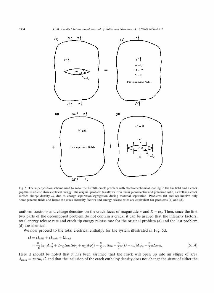
Fig. 5. The superposition scheme used to solve the Griffith crack problem with electromechanical loading in the far field and a crack

gap that is able to store electrical energy. The original problem (a) allows for a linear piezoelectric and polarized solid, as well as a crack

surface charge density xs due to charge separation/segregation during material separation. Problems (b) and (c) involve only

homogeneous fields and hence the crack intensity factors and energy release rates are equivalent for problems (a) and (d).


uniform tractions and charge densities on the crack faces of magnitude r and D� xs. Then, since the first

two parts of the decomposed problem do not contain a crack, it can be argued that the intensity factors,total energy release rate and crack tip energy release rate for the original problem (a) and the last problem

(d) are identical.

We now proceed to the total electrical enthalpy for the system illustrated in Fig. 5d.

X ¼ Xsolid þ Xloads þ Xcrack

¼ p16

ðg11Du20 þ 2g12Du0D/0 þ g22D/20Þ �

p2arDu0 �

p2aðD� xsÞD/0 þ

p2aDu0hc ð5:14Þ

Here it should be noted that it has been assumed that the crack will open up into an ellipse of areaAcrack ¼ paDu0=2 and that the inclusion of the crack enthalpy density does not change the shape of either the


crack opening displacement or electric potential drop distributions. Note, however, that the inclusion of the

crack enthalpy density can change the sizes of these distributions.

It is now assumed, in a fashion consistent with Eq. (2.12), that the solution to this problem causes the

total electrical enthalpy to be stationary. Eq. (5.14) has expanded the electrical enthalpy into a function oftwo unknown scalar variables Du0 and D/0. Therefore, the following equations must be satisfied for the

solution

oXoDu0

¼ p8ðg11Du0 þ g12D/0Þ �

p2arþ p

2arc ¼ 0 ð5:15Þ

oXoD/0

¼ p8ðg12Du0 þ g22D/0Þ �

p2aðD� xsÞ þ

p2aDc ¼ 0 ð5:16Þ

Along with the definition rc ¼ hc þ EcDc, the following relationships have been used to derive the simplified

forms of Eqs. (5.15) and (5.16).

ohcoDu0

¼ dhcdEc

oEc

oDu0¼ �Dc

o

oDu0

�� D/0

Du0

�¼ �Dc

D/0

Du20¼ EcDc

1

Du0ð5:17Þ

ohcoD/0

¼ dhcdEc

oEc

oD/0

¼ �Dc

o

oD/0

�� D/0

Du0

�¼ Dc

1

Du0ð5:18Þ

In general, both rc and Dc are non-linear functions of Du0 and D/0 and hence Eqs. (5.15) and (5.16)

represent a set of non-linear equations governing Du0 and D/0. Explicit solutions to these equations will be

detailed later in this subsection. However, (5.15) and (5.16) can be readily manipulated to demonstrate

some features of the solution.

First, by inverting the first terms of Eqs. (5.15) and (5.16), the crack opening displacement and electric

potential drop across the crack can be shown to be

Du0 ¼ 4a½H11ðr� rcÞ þ H12ðD� xs � DcÞ� ð5:19Þ

D/0 ¼ 4a½H12ðr� rcÞ þ H22ðD� xs � DcÞ� ð5:20Þ

Note that this solution can be interpreted as the solution in the solid material with r� ¼ r� rc and

D� ¼ D� xs � Dc. Hence, the intensity factors and the crack tip energy release rate are given as

KI ¼ ðr� rcÞffiffiffiffiffiffipa

pð5:21Þ

KD ¼ ðD� xs � DcÞffiffiffiffiffiffipa

pð5:22Þ

Gtip ¼ pa½H11ðr� rcÞ2 þ 2H12ðr� rcÞðD� xs � DcÞ þ H22ðD� xs � DcÞ2� ð5:23Þ

Note that the intensity factors KI and KD depend on the features of the energetically consistent boundary

conditions rc and Dc. Furthermore, the levels of rc and Dc are dependent on KI and KD as will be detailed

later in this section. A more detailed discussion of this coupling that arises from the energetically consistent

boundary conditions and its effects on the asymptotic crack tip fields in linear piezoelectric solids is included

in Appendix B.

Returning to the Griffith crack problem, by adding Eq. (5.15) multiplied by Du0 with Eq. (5.16) mul-

tiplied by D/0, it can be shown that

g11Du20 þ 2g12Du0D/0 þ g22D/

20 ¼ 4aðr� rcÞDu0 þ 4aðD� xs � DcÞD/0 ð5:24Þ


Then, implementing Eqs. (5.19), (5.20) and (5.24), the equation for the total electrical enthalpy can be

manipulated as

X ¼ p16

ðg11Du20 þ 2g12Du0D/0 þ g22D/20Þ �

p2arDu0 �


p2aDu0hc

¼ p4a½ðr� rcÞDu0 þ 4aðD� xs � DcÞD/0� �

p2arDu0 �

p2aðD� xsÞD/0

þ p2aDu0 hc

�þ EcDc þ Dc

D/0

Du0

�

¼ p4a½ðr� rcÞDu0 þ 4aðD� xs � DcÞD/0� �

p2arDu0 �


p2arcDu0 þ

p2aDcD/0

¼ � p4a½ðr� rcÞDu0 þ ðD� xs � DcÞD/0�

¼ �pa2½H11ðr� rcÞ2 þ 2H12ðr� rcÞðD� xs � DcÞ þ H22ðD� xs � DcÞ2� ð5:25Þ

Now, recognizing that the total energy release rate per unit of crack advance for one of the crack tips is

given by the opposite of the derivative of the electrical enthalpy with respect to the total crack length 2a,Gtotal can be shown to be

Gtotal ¼ � oXoð2aÞ ¼ pa½H11ðr� rcÞ2 þ 2H12ðr� rcÞðD� xs � DcÞ þ H22ðD� xs � DcÞ2� ð5:26Þ

Therefore, it has now been shown that the total energy release rate is equal to the crack tip energy release

rate for this system with any arbitrary form of the electrical enthalpy density for the crack medium. For the

remainder of this paper both Gtip and Gtotal will simply be referred to as the energy release rate G whenapplying the energetically consistent boundary conditions. Also, note that this solution procedure applies

the weak form of the governing equations and that the crack face boundary conditions derived in Section 3

were not applied directly. However, if the strong form of the equations had been applied with the crack

boundary conditions of Section 3, the solution that would have been obtained would be identical to that

outlined above. We now proceed to a few specific examples.

First, Eqs. (5.15) and (5.16) will be solved for the case where the electrical enthalpy density of the crack

medium is given by that described in Section 3.2. Specifically, the solution to Eqs. (5.15) and (5.16) can be

obtained by the following procedure. If the electric field supported by the crack gap is less than the dis-charge field Ed, then the crack opening displacement is governed by the following cubic equation,

g11Du0a

g22Du0a

�� 4j0

�2

� g12Du0a

g12Du0a

�� 4ðD� xsÞ

�g22

Du0a

�� 4j0

�

þ 2j0 g12Du0a

�� 4ðD� xsÞ

�2� 4r g22

Du0a

�� 4j0

�2

¼ 0 ifD/0

Du0

��6Ed ð5:27Þ

After obtaining the relevant solution to Eq. (5.27), the potential drop across the crack is given by

D/0 ¼ j20Du0

4ðD� xsÞa� g12Du04j0a� g22Du0

ifD/0

Du0

��6Ed ð5:28Þ

Fig. 6 is a contour plot of the solutions for the energy release rate (total or crack tip) predicted using the

energetically consistent boundary conditions assuming no electrical discharge for wide ranges of applied

stress r and effective electric displacement D� xs. The material properties of the linear piezoelectric

material are characteristic of PZT-5H and are listed in Appendix A. The results of Fig. 6 are valid for either

polar or non-polar materials. However, for polar materials D ¼ DDþ P r. It is common to present resultslike those shown in Fig. 6 with the abscissa as electric field instead of D� xs. However, such a presentation

landis

Rectangle

landis

Text Box

_

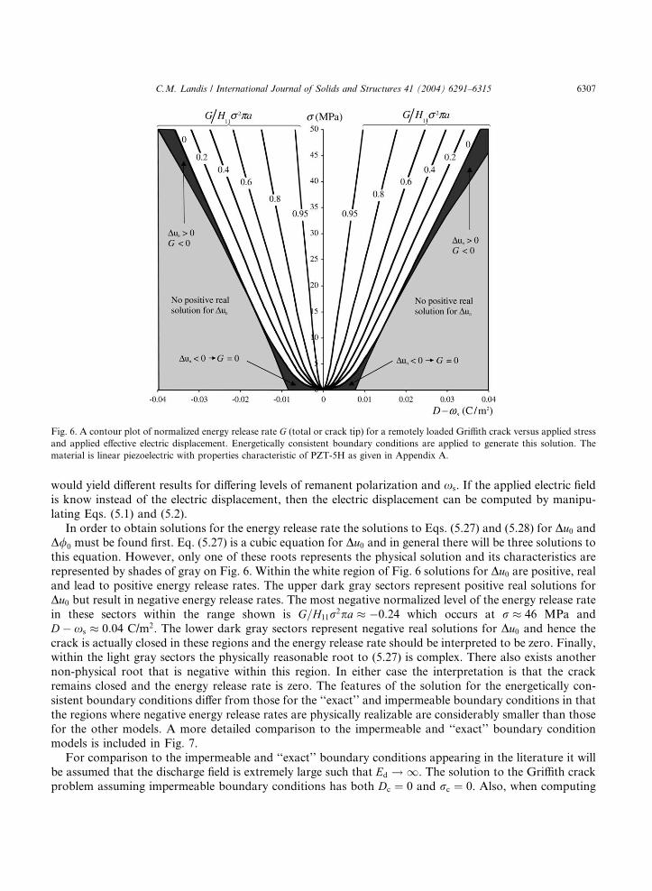
Fig. 6. A contour plot of normalized energy release rate G (total or crack tip) for a remotely loaded Griffith crack versus applied stress

and applied effective electric displacement. Energetically consistent boundary conditions are applied to generate this solution. The

material is linear piezoelectric with properties characteristic of PZT-5H as given in Appendix A.


would yield different results for differing levels of remanent polarization and xs. If the applied electric field

is know instead of the electric displacement, then the electric displacement can be computed by manipu-

lating Eqs. (5.1) and (5.2).

In order to obtain solutions for the energy release rate the solutions to Eqs. (5.27) and (5.28) for Du0 andD/0 must be found first. Eq. (5.27) is a cubic equation for Du0 and in general there will be three solutions to

this equation. However, only one of these roots represents the physical solution and its characteristics are

represented by shades of gray on Fig. 6. Within the white region of Fig. 6 solutions for Du0 are positive, realand lead to positive energy release rates. The upper dark gray sectors represent positive real solutions for

Du0 but result in negative energy release rates. The most negative normalized level of the energy release rate

in these sectors within the range shown is G=H11r2pa � �0:24 which occurs at r � 46 MPa and

D� xs � 0:04 C/m2. The lower dark gray sectors represent negative real solutions for Du0 and hence the

crack is actually closed in these regions and the energy release rate should be interpreted to be zero. Finally,within the light gray sectors the physically reasonable root to (5.27) is complex. There also exists another

non-physical root that is negative within this region. In either case the interpretation is that the crack

remains closed and the energy release rate is zero. The features of the solution for the energetically con-

sistent boundary conditions differ from those for the ‘‘exact’’ and impermeable boundary conditions in that

the regions where negative energy release rates are physically realizable are considerably smaller than those

for the other models. A more detailed comparison to the impermeable and ‘‘exact’’ boundary condition

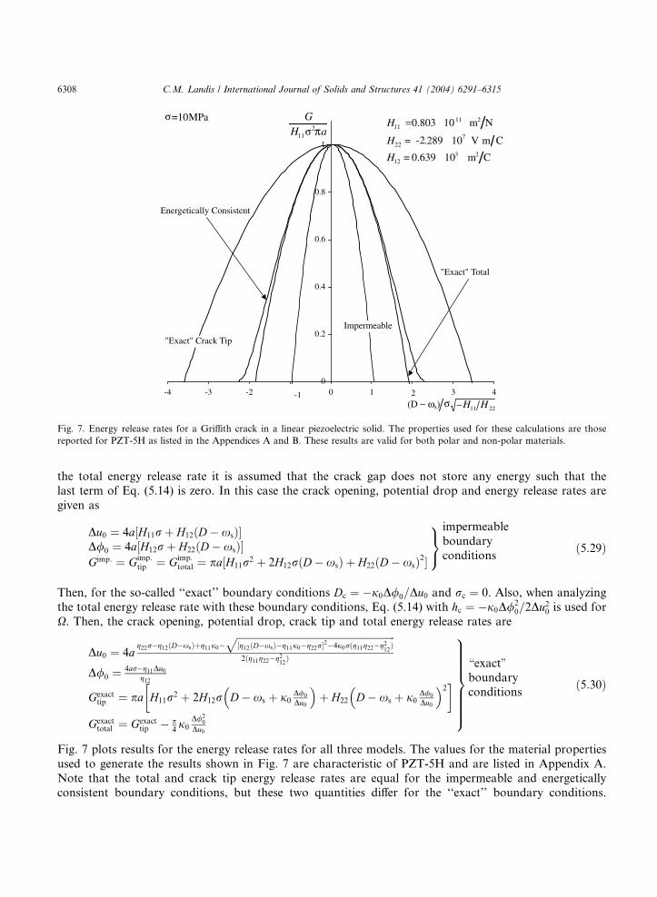
models is included in Fig. 7.

For comparison to the impermeable and ‘‘exact’’ boundary conditions appearing in the literature it willbe assumed that the discharge field is extremely large such that Ed ! 1. The solution to the Griffith crack

problem assuming impermeable boundary conditions has both Dc ¼ 0 and rc ¼ 0. Also, when computing

0

0.2

0.4

0.6

0.8

1

-4 -3 -2 -1 0 1 2 3 4

"Exact" Crack Tip

Energetically Consistent

"Exact" Total

Impermeable

H11 =0.803 1011 m2 N

H22 = -2.289 107 V m C

H12 = 0.639 103 m2 C

=10 MPa

s H11 H 22

GH11

2πa

σ

σσ

(D − ω ) −

Fig. 7. Energy release rates for a Griffith crack in a linear piezoelectric solid. The properties used for these calculations are those

reported for PZT-5H as listed in the Appendices A and B. These results are valid for both polar and non-polar materials.


the total energy release rate it is assumed that the crack gap does not store any energy such that the

last term of Eq. (5.14) is zero. In this case the crack opening, potential drop and energy release rates are

given as

Du0 ¼ 4a½H11rþ H12ðD� xsÞ�D/0 ¼ 4a½H12rþ H22ðD� xsÞ�Gimp: ¼ Gimp:

tip ¼ Gimp:total ¼ pa½H11r2 þ 2H12rðD� xsÞ þ H22ðD� xsÞ2�

9=;

impermeable

boundary

conditionsð5:29Þ

Then, for the so-called ‘‘exact’’ boundary conditions Dc ¼ �j0D/0=Du0 and rc ¼ 0. Also, when analyzing

the total energy release rate with these boundary conditions, Eq. (5.14) with hc ¼ �j0D/20=2Du

20 is used for

X. Then, the crack opening, potential drop, crack tip and total energy release rates are

Du0 ¼ 4ag22r�g12ðD�xsÞþg11j0�

ffiffiffiffiffiffiffiffiffiffiffiffiffiffiffiffiffiffiffiffiffiffiffiffiffiffiffiffiffiffiffiffiffiffiffiffiffiffiffiffiffiffiffiffiffiffiffiffiffiffiffiffiffiffiffiffiffiffiffiffiffiffiffi½g12ðD�xsÞ�g11j0�g22r�2�4j0rðg11g22�g2

12Þ

p2ðg11g22�g2

12Þ

D/0 ¼ 4ar�g11Du0g12

Gexacttip ¼ pa H11r2 þ 2H12r D� xs þ j0

D/0

Du0

� �þ H22 D� xs þ j0

D/0

Du0

� �2� �

Gexacttotal ¼ Gexact

tip � p4j0

D/20

Du0

9>>>>>>>=>>>>>>>;

\exact"boundary

conditionsð5:30Þ

Fig. 7 plots results for the energy release rates for all three models. The values for the material properties

used to generate the results shown in Fig. 7 are characteristic of PZT-5H and are listed in Appendix A.

Note that the total and crack tip energy release rates are equal for the impermeable and energeticallyconsistent boundary conditions, but these two quantities differ for the ‘‘exact’’ boundary conditions.


Furthermore, note that the crack tip energy release rates are computed from Eq. (5.6), whereas the total

energy release rates are computed from Gtotal ¼ �oX=oð2aÞ. As for Fig. 6, the results of Fig. 7 are valid for

either polar or non-polar materials.

Fig. 7 illustrates a number of interesting features of this problem. First, for the modest applied stresslevel of 10-MPa the difference between the crack tip energy release rate and the total energy release rate for

the ‘‘exact’’ boundary conditions that are so prevalent in the literature is significant over a wide range of

D� xs. Furthermore, the simple fact that these two quantities differ, regardless of the magnitude of the

difference, is unappealing from a theoretical perspective. It is also interesting to note that both the ‘‘exact’’

and energetically consistent boundary conditions yield energy release rates significantly higher than the

energy release rate for the impermeable boundary conditions. This feature arises because the existence of

cracks in the presence of electric fields tends to be a high-energy state and hence electric fields tend to retard

crack growth and the energy released during crack growth. This retardation process is maximized for theimpermeable boundary conditions, but reduced for the ‘‘exact’’ and energetically consistent boundary

conditions where electric fields can permeate through the crack gap. Finally, the energy release rate for the

energetically consistent boundary conditions is higher than the total energy release rate for the ‘‘exact’’

boundary conditions. This result may seem counterintuitive since in addition to allowing for electric fields

within the crack gap, the energetically consistent boundary conditions also include a closing traction on the

crack faces. One would expect that the closing traction should further reduce the energy release rate.

However, recall that the energetically consistent boundary conditions cause the electrical enthalpy to be

stationary, and this is equivalent to minimizing the potential energy P of the system. Recall that for thespecific case of the Griffith crack problem Gtotal ¼ �oX=oð2aÞ ¼ �oP=oð2aÞ ¼ �P=a. Therefore, the

solution that minimizes P will maximize the total energy release rate.

One final observation from the solutions presented in Fig. 7 is that the electric field in the crack gap is

much larger than the level of electric field applied to the solid. This feature of the solution, along with

experimental observations of discharge in crack gaps, is the motivation to study the effects of electrical

discharge on the energy release rate for this system. In order to determine if (5.27) and (5.28) yield the valid

solution, the condition that the electric field in the crack gap is less than the discharge field, jD/0=Du0j6Ed,

must be verified. If the solution to (5.27) and (5.28) yields jD/0=Du0j > Ed then the solutions for the crackopening displacement, potential drop, and level of discharge are given as

Du0 ¼ 4ar� ðD� xsÞsgnðxdÞEd þ j0E2

d=2

g11 � 2g12sgnðxdÞEd þ g22E2d

if jxdj > 0 ð5:31Þ

D/0 ¼ �sgnðxdÞEdDu0 ¼ �4asgnðxdÞEd

r� ðD� xsÞsgnðxdÞEd þ j0E2d=2


if jxdj > 0 ð5:32Þ

xd ¼ D� xs � j0sgnðxdÞEd � ðg12 � g22sgnðxdÞEdÞr� ðD� xsÞsgnðxdÞEd þ j0E2

d=2


if jxdj > 0

ð5:33Þ

Eq. (5.33) can be used to check the consistency for the choice of sgnðxdÞ. If neither sgnðxdÞ ¼ 1 nor

sgnðxdÞ ¼ �1 is consistent with Eq. (5.33) then this most likely implies the electric field in the gap is less

than the critical discharge field and Eqs. (5.27) and (5.28) should be used for the solution. However, a

second scenario can arise if the magnitude of the discharge field is greater than either the positive ornegative critical levels defined by

Ecrit�d ¼ �H12 �

ffiffiffiffiffiffiffiffiffiffiffiffiffiffiffiffiffiffiffiffiffiffiffiffiffiffiffiH 2

12 � H11H22

pH11

�� ð5:34Þ


If the discharge field is greater than the appropriate critical level then consistent solutions for the crack

opening and electric displacement within the crack cannot be obtained when the electric field within the

crack reaches the discharge level. The most likely physical interpretation is that the system is unstable when

the electric field within the crack attains the discharge level. For the remainder of this section it will beassumed that the discharge field is less than both of the critical levels from (5.34).

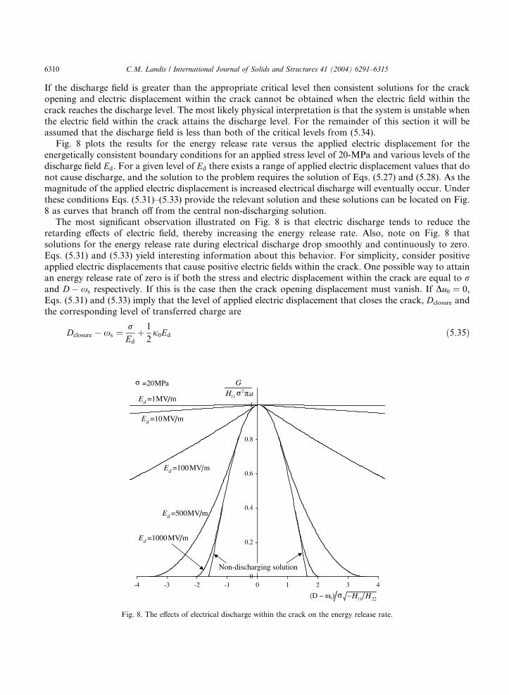
Fig. 8 plots the results for the energy release rate versus the applied electric displacement for the

energetically consistent boundary conditions for an applied stress level of 20-MPa and various levels of the

discharge field Ed. For a given level of Ed there exists a range of applied electric displacement values that do

not cause discharge, and the solution to the problem requires the solution of Eqs. (5.27) and (5.28). As the

magnitude of the applied electric displacement is increased electrical discharge will eventually occur. Under

these conditions Eqs. (5.31)–(5.33) provide the relevant solution and these solutions can be located on Fig.

8 as curves that branch off from the central non-discharging solution.The most significant observation illustrated on Fig. 8 is that electric discharge tends to reduce the

retarding effects of electric field, thereby increasing the energy release rate. Also, note on Fig. 8 that

solutions for the energy release rate during electrical discharge drop smoothly and continuously to zero.

Eqs. (5.31) and (5.33) yield interesting information about this behavior. For simplicity, consider positive

applied electric displacements that cause positive electric fields within the crack. One possible way to attain

an energy release rate of zero is if both the stress and electric displacement within the crack are equal to rand D� xs respectively. If this is the case then the crack opening displacement must vanish. If Du0 ¼ 0,

Eqs. (5.31) and (5.33) imply that the level of applied electric displacement that closes the crack, Dclosure andthe corresponding level of transferred charge are

Dclosure � xs ¼rEd

þ 1

2j0Ed ð5:35Þ

0

0.2

0.4

0.6

0.8

1

-4 -3 -2 -1 0 1 2 3 4

=20 MPa

Ed =1MV m

Ed =10MV m

Ed =100MV m

Ed =500MV m

Ed =1000MV m

Non-discharging solution

GH11

2πa

s H11 H 22σ

σσ

(D − ω ) −

Fig. 8. The effects of electrical discharge within the crack on the energy release rate.


xd ¼ Dclosure � xs � j0Ed ¼rEd

� 1

2j0Ed ð5:36Þ

Then, it is readily shown that

Dc ¼ xd þ j0Ed ¼rEd

þ 1

2j0Ed ¼ Dclosure � xs ð5:37Þ

and

rc ¼ DcEd �1

2j0E2

d ¼ rþ 1

2j0E2

d �1

2j0E2

d ¼ r ð5:38Þ

Therefore, if the crack is closed then the stress and electric displacement within the gap are equal to the

associated applied levels. Finally, applying Eq. (5.23) or (5.26) it can be shown that G ¼ 0 under these

conditions. Hence, the level of effective electric displacement where the energy release rate is zero corre-

sponds to the point where the crack is closed. Levels of effective electric displacement higher than the

closure level given in Eq. (5.35) only act to close the crack further. Therefore, since the crack cannotphysically be closed beyond Du0 ¼ 0, this electrical discharging crack model cannot lead to negative energy

release rates if the discharge field is less than the critical values given in Eq. (5.34).

6. Discussion

This work has been motivated primarily by McMeeking’s observation, McMeeking (2004), that the so-called ‘‘exact’’ electrical boundary conditions that are prevalent in the literature give rise to a discrepancy

between the total and crack tip energy release rates in a cracked piezoelectric body. Such a discrepancy is

objectionable from a theoretical perspective. To address this problem, energetically consistent electro-

mechanical boundary conditions for cracks were derived in Section 3. These boundary conditions were

derived based on the following assumptions. (1) The energy of the cracked body can be computed using its

undeformed configuration. (2) When the crack opens electric fields can permeate the crack medium and

electrical energy can be stored within the crack. (3) The energy stored within the crack medium can be

computed from the deformed configuration of the cracked body. (4) Electric field components within thecrack medium parallel to the crack faces are negligible compared to the electric field normal to the crack.

Evidently, assumptions (1) and (3) are in contradiction with one another since the analysis of energies is

mixed between deformed and undeformed configurations. However, these assumptions are consistent with

those used for the ‘‘exact’’ boundary conditions. Furthermore, a proper resolution to this inconsistency

would require a full non-linear, large deformation kinematics analysis of the problem. Instead, in this work,

assumptions (1)–(4) are taken as a starting point and the energetically consistent crack boundary conditions

are derived by equating the weak statements of two boundary value problems; one which models the

volume of the crack gap explicitly and one that models the crack gap through the surface tractions andcharges that it applies to the cracked solid.

The primary results of this paper are the energetically consistent boundary conditions given by Eqs.

(3.11)–(3.14). These boundary conditions imply that cracks in electromechanical materials not only sustain

electric field and electric displacement, but also apply mechanical traction to the surrounding material. This

feature of mechanical forces arising due to electrical effects is common in finite deformation analyses of

electromechanical materials and is usually termed a Maxwell stress. With these energetically consistent

boundary conditions, Section 4 was used to demonstrate that a small modification to the J -integral could be

used to compute the energy release rate for crack advance in a non-linear but reversible electromechanicalsolid. The results of Sections 3 and 4 will be especially useful for the analysis of cracked piezoelectric bodies

with the finite element method. McMeeking (1999) and Gruebner et al. (2003) have already implemented


the finite element method with the ‘‘exact’’ boundary conditions. Similar computations can readily be

performed with the new energetically consistent boundary conditions and the modified J -integral of Section4 can be used to determine the energy release rate within these types of calculations. Finally, in Section 5,

the specific example of a Griffith crack in a poled linear piezoelectric solid was used to demonstrate that theenergetically consistent boundary conditions do in fact resolve the discrepancy between the crack tip and

total energy release rates. Furthermore, the effects of electrical discharge on the energy release rate was

ascertained and shown to reduce the retarding effects of electric fields on crack growth.

Acknowledgement

The author would like to acknowledge support for this work from the National Science Foundationthrough grant number CMS-0238522.

Appendix A

The treatment of the Griffith crack problem outlined in Section 5 assumes that the components of theIrwin matrix for the material are known. Irwin matrices are given in this appendix for PZT-5H as reported

by McMeeking (2004) and for materials with a special form of simplified piezoelectric properties as given by

Landis (2004).

For PZT-5H, McMeeking (2004) reports the following piezoelectric coefficients for a material that is

poled and transversely isotropic about the x3-axis.

cE1111 ¼ 126 GPa; cE1122 ¼ 55 GPa; cE1133 ¼ 53 GPa; cE3333 ¼ 117 GPa; cE2323 ¼ 35:3 GPa

e311 ¼ �6:5 C=m2; e333 ¼ 23:3 C=m2; e113 ¼ 17 C=m2

je11 ¼ 15:1� 10�9 C=Vm; je

33 ¼ 13� 10�9 C=Vm

Then, the Irwin matrix for PZT-5H poled in the x2 direction under plane strain conditions is

H11 H12

H12 H22

� �¼ 0:803� 10�11 m2=N 0:639� 10�3 m2=C

0:639� 10�3 m2=C �2:289� 107 Vm=C

� �ðA:1Þ

Of course, this result for the Irwin matrix is applicable only to PZT-5H, and in order to obtain results for a

different material the associated Irwin matrix needs to be determined. This can be accomplished by fol-

lowing the procedure described by McMeeking (2004) among others. On the other hand, if the material

properties can be reasonably approximated with the following description due to Landis (2004) then the

Irwin matrix can be obtained in closed form.

Specifically, if the elastic compliance and dielectric permittivity tensors can be assumed to be isotropic

and the piezoelectric d coefficients satisfy transversely isotropic symmetries and d113 ¼ ðd333 � d311Þ=2, thenthe non-zero strain and electric displacement components due to electromechanical loading in the 1–3 plane

for a material poled in the x3 direction are given as

e11 ¼1

Er11 �

mEr22 �

mEr33 þ d311E3 ðA:2Þ

e22 ¼ � mEr11 þ

1

Er22 �

mEr33 þ d311E3 ðA:3Þ


e33 ¼ � mEr11 �

mEr22 þ

1

Er33 þ d333E3 ðA:4Þ

e13 ¼1þ mE

r13 þd333 � d311

2E1 ðA:5Þ

D1 ¼ ðd333 � d311Þr13 þ jE1 ðA:6Þ

D3 ¼ d311r11 þ d311r22 þ d333r33 þ jE3 þ P r3 ðA:7Þ

Here E and m are the isotropic Young’s modulus and Poisson’s ratio at constant electric field, j is the

isotropic dielectric permittivity at constant stress, and d333 and d333 are piezoelectric coefficients. Then, the

Irwin matrix for such a material poled in the x2 direction in plane strain is

ðA:8Þ

where d33 ¼ d333, d31 ¼ d311, d15 ¼ d333 � d311,

DD ¼ keð1� mÞ þ 2ðae � 1Þð1þ mÞ; DE ¼ keaeð1� mÞ þ 2ðae � 1Þð1þ mÞ;

ke ¼2Ed2

31

jð1� mÞ and ae ¼

ffiffiffiffiffiffiffiffiffiffiffiffi1

1� ke

s:

For plane stress the Irwin matrix for this material is

ðA:9Þ

where kr ¼Ed2

31

j and ar ¼ffiffiffiffiffiffiffi1

1�kr

q.

Appendix B

In this appendix the effects of the energetically consistent boundary conditions on the first two terms of

the asymptotic expansion for the solutions near crack tips in linear piezoelectric solids are outlined. It is

expected that the non-singular T terms will have an effect on the sizes and shapes of switching zones near

crack tips in non-linear ferroelectric materials. As in Section 5 simplicity is sought by considering onlymixed Modes I and D loading. The inclusion of Modes II and III would require additional singular Kterms, but the non-singular T terms would remain unchanged. Under mixed Mode I and Mode D the

Cartesian components of the stresses and electric displacements near a crack tip in a linear piezoelectric

solid can be expanded into the forms

rijðr; hÞ ¼KIffiffiffiffiffiffiffi2pr

p ~rIijðhÞ þ

KDffiffiffiffiffiffiffi2pr

p ~rDijðhÞ þ T r

ij þ Oðffiffir

pÞ ðB:1Þ

Diðr; hÞ ¼KIffiffiffiffiffiffiffi2pr

p ~DIi ðhÞ þ

KDffiffiffiffiffiffiffi2pr

p ~DDi ðhÞ þ TD

i þ Oðffiffir

pÞ ðB:2Þ


Here r and h are polar coordinates as illustrated in Fig. 2, and ~rIijðhÞ ¼ ~rI

jiðhÞ, ~rDijðhÞ ¼ ~rD

jiðhÞ, ~DIi ðhÞ and

~DDi ðhÞ are dimensionless functions of h that satisfy the following boundary conditions,

~rI22ðh ¼ 0Þ ¼ ~DD

2 ðh ¼ 0Þ ¼ 1 ðB:3Þ

~rD22ðh ¼ 0Þ ¼ ~rI

12ðh ¼ 0Þ ¼ ~rD12ðh ¼ 0Þ ¼ ~rI

23ðh ¼ 0Þ ¼ ~rD23ðh ¼ 0Þ ¼ ~DI

2ðh ¼ 0Þ ¼ 0 ðB:4Þ

~rI22ðh ¼ �pÞ ¼ ~rI

12ðh ¼ �pÞ ¼ ~rI23ðh ¼ �pÞ ¼ ~DD

2 ðh ¼ �pÞ ¼ 0 ðB:5Þ

~rD22ðh ¼ �pÞ ¼ ~rD

12ðh ¼ �pÞ ¼ ~rD23ðh ¼ �pÞ ¼ ~DI

2ðh ¼ �pÞ ¼ 0 ðB:6Þ

Notice that the boundary conditions represented by Eqs. (B.5) and (B.6) are the same as those associated

with the impermeable crack model. Hence, the impermeable crack boundary conditions are valid for the

singular K terms, and standard methods can be applied to determine the dimensionless stress and electric

displacement functions, e.g. Suo et al. (1992).

The direct effects of the energetically consistent boundary conditions first arise in the non-singular Tterms. Near the crack tip the jumps in displacement and electric potential across the crack are given as

Du2 ¼ u2ðr; h ¼ pÞ � u2ðr; h ¼ �pÞ ¼ 4

ffiffiffiffiffi2rp

rðH11KI þ H12KDÞ þ Oðr3=2Þ ðB:7Þ

D/ ¼ /ðr; h ¼ pÞ � /ðr; h ¼ �pÞ ¼ 4

ffiffiffiffiffi2rp

rH12KIð þ H22KDÞ þ Oðr3=2Þ ðB:8Þ

where the H terms are the components of the Irwin matrix as given in Appendix A. Then the electric field in

the crack gap is given as

Ec ¼ � D/Du2

¼ �H11KI þ H12KD

H12KI þ H22KD

þ OðrÞ ðB:9Þ

which is independent of r to leading order near the crack tip. This implies that the electric displacement and

the stress acting through the crack gap are constant to leading order near the crack tip as well and are givenby

Dc ¼ � dhcdEc

and rc ¼ hc þ EcDc ðB:10Þ

Then, in order to satisfy the energetically consistent boundary conditions, the T terms must satisfy the

conditions

T r22 ¼ rc; TD

2 ¼ Dc; and T r12 ¼ T r

21 ¼ T r23 ¼ T r

32 ¼ 0 ðB:11Þ

The remaining terms T r11, T

r33, T

r13 ¼ T r

31, TD1 and TD

3 take on values as determined from the geometry of the

cracked body and the applied electromechanical loading.

Finally, it is important to note that there is a coupling between the singular K terms and the non-singular

T terms when applying the energetically consistent boundary conditions. Specifically, the dependence of T r22

and T D2 on KI and KD is demonstrated by Eqs. (B.9)–(B.11), whereas KI and KD depend on T r

22 and TD2 (i.e. rc

and Dc) through the details of the boundary value problem as illustrated for the Griffith crack problem in

Eqs. (5.21) and (5.22).


References

Chen, Y.-H., Lu, T.J., 2002. Cracks and fracture in piezoelectrics. Adv. Appl. Mech. 39, 121–215.

Deeg, W.F., 1980. The analysis of dislocation, crack and inclusion problems in piezoelectric solids. Ph.D. Thesis, Stanford University.

Gruebner, O., Kamlah, M., Munz, D., 2003. Finite element analysis of cracks in piezoelectrics taking into account the permittivity of

the crack medium. Eng. Fract. Mech. 70, 1399–1413.

Hao, T.-H., Shen, Z.-Y., 1994. A new electric boundary condition of electric fracture mechanics and its application. Eng. Fract. Mech.

47, 793–802.

Landis, C.M., 2004. In-plane complex potentials for a special class of materials with degenerate material properties. Int. J. Solids

Struct. 41, 695–715.

Landis, C.M., McMeeking, R.M., 2000. Modeling of fracture in ferroelectric ceramics. Proc. SPIE 3992, 176–184.

Li, J.C.M., Ting, T.W., 1957. Thermodynamics for elastic solids in the electrostatic field. I. General formulation. J. Chem. Phys.

27, 693–700.

McMeeking, R.M., 1999. Crack tip energy release rate for a piezoelectric compact tension specimen. Eng. Fract. Mech. 64, 217–244.

McMeeking, R.M., 2004. The energy release rate for a Griffith crack in a piezoelectric material. Eng. Fract. Mech. 71, 1149–1163.

Pak, Y.E., 1992. Linear electro-elastic fracture mechanics of piezoelectric materials. Int. J. Fract. 54, 79–100.

Parton, V.Z., 1976. Fracture mechanics of piezoelectric materials. Acta Astronautica 3, 671–683.

Sosa, H., 1992. On the fracture mechanics of piezoelectric solids. Int. J. Solids Struct. 29, 2613–2622.

Sosa, H., Khutoryansky, N., 1996. New developments concerning piezoelectric materials with defects. Int. J. Solids Struct. 33, 3399–

3414.

Suo, Z., Kuo, C.M., Barnett, D.M., Willis, J.R., 1992. Fracture mechanics for piezoelectric ceramics. J. Mech. Phys. Solids 40, 739–

765.

Xu, X.L., Rajapakse, R.K.N.D., 2001. On a plane crack in piezoelectric solids. Int. J. Solids Struct. 38, 7643–7658.

Zhang, T.Y., Gao, C.F., 2004. Fracture behaviors of piezoelectric materials. Theor. Appl. Fract. Mech. 41, 339–379.

Zhang, T.-Y., Zhao, M., Tong, P., 2001. Fracture of piezoelectric ceramics. Adv. Appl. Mech. 38, 147–289.

Corrigendum

Energetically consistent boundary conditionsfor electromechanical fracture [International Journal of

Solids and Structures 41 (2004) 6291–6315]

Chad M. Landis *

Mechanical Engineering and Materials Science, P.O. Box 1892, Houston, TX 77251 1892, United States

Received 9 August 2004Available online 27 October 2004

The author regrets a transcription error in a quantity used for the numerical results presented in Figs. 6–8. Eq. (A.1) of Appendix A reports that the Irwin matrix for PZT-5H poled in the x2 direction under planestrain conditions is

H 11 H 12

H 12 H 22

� �¼ 0:803� 10�11m2=N 0:639� 10�3m2=C

0:639� 10�3m2=C �2:289� 107 Vm=C

" #ðIncorrect for PZT� 5HÞ ðA:1Þ

where the material properties (if poled in the x3 direction) used to derive this matrix are

cE1111 ¼ 126GPa; cE1122 ¼ 55GPa; cE1133 ¼ 53GPa; cE3333 ¼ 117GPa; cE2323 ¼ 35:3GPa

e311 ¼ �6:5C=m2; e333 ¼ 23:3C=m2; e113 ¼ 17C=m2

je11 ¼ 15:1� 10�9 C=Vm; je

33 ¼ 13� 10�9 C=Vm

The error occurs in the H12 term, which should be 6.39 · 10�3 instead of 0.639 · 10�3. Hence the correctIrwin matrix for PZT-5H is

H 11 H 12

H 12 H 22

� �¼ 0:803� 10�11m2=N 6:39� 10�3m2=C

6:39� 10�3m2=C �2:289� 107 Vm=C

" #ðCorrect for PZT� 5HÞ ðA:1Þ

The corrected numerical results presented in Figs. 6–8 are as follows. Note that the qualitative discussion ofeach of these figures is unaffected by this error.

Note that a publishing error occurred in the original Fig. 7. Minus signs are missing on the exponents inthe H11 and H12 terms appearing on the figure inset, and an ‘‘·’’ does not appear prior to the 10�s.

0020-7683/$ - see front matter � 2004 Elsevier Ltd. All rights reserved.doi:10.1016/j.ijsolstr.2004.09.017

DOI of original article 10.1016/j.ijsolstr.2004.05.062.* Tel.: +1 713 3483 609; fax: +1 713 3485 423.E-mail address: [email protected]

International Journal of Solids and Structures 42 (2005) 2461–2463

www.elsevier.com/locate/ijsolstr

Fig. 6. A contour plot of normalized energy release rate G (total or crack tip) for a remotely loaded Griffith crack versus applied stressand applied effective electric displacement. Energetically consistent boundary conditions with no discharge allowed are applied togenerate this solution. The material is linear piezoelectric with properties characteristic of PZT-5H and the Irwin matrix as correctedabove.

Fig. 7. Energy release rates for a Griffith crack in a linear piezoelectric solid with no discharge in the crack allowed. The propertiesused for these calculations are those reported for PZT-5H and the Irwin matrix as corrected above. These results are valid for bothpolar and non-polar materials.

2462 Corrigendum / International Journal of Solids and Structures 42 (2005) 2461–2463

Finally, the results presented in the original manuscript are in fact valid for a material with the Irwinmatrix as first reported. However, such an Irwin matrix does not result from the material properties forPZT-5H as reported in the manuscript and above. One set of material properties that does yield this orig-inal Irwin matrix to within 0.2% for each term is

cE1111 ¼ cE3333 ¼ 152:1GPa; cE1122 ¼ cE1133 ¼ 65:19GPa; cE2323 ¼ 43:46 GPa

e311 ¼ �1:428C=m2; e333 ¼ 2:855C=m2; e113 ¼ 2:142C=m2

je11 ¼ 21:75� 10�9 C=Vm; je

33 ¼ 21:79� 10�9 C=Vm

Hence, the originally reported results are valid for such a piezoelectric material.The author sincerely apologizes for any confusion or difficulties this error may have caused.

Fig. 8. The effects of electrical discharge within the crack on the energy release rate. Results are reported only for the energeticallyconsistent boundary conditions. The properties used for these calculations are those reported for PZT-5H and the Irwin matrix ascorrected above.

Corrigendum / International Journal of Solids and Structures 42 (2005) 2461–2463 2463

energetically consistent boundary conditions for electromechanical

Documents