1

Preliminary and Incomplete

Endowments, Investments and the Development of Human Capital

Anna Aizer* Brown University and NBER

Flavio Cunha

University of Pennsylvania and NBER

March 2011

We study how initial levels of human capital, parental investments and fertility interact to produce human capital in childhood. We being with an exploration the mechanics of the production function; specifically, whether initial human capital and investments are complements in the production of later human capital. We exploit an exogenous source of investment, the launch of Head Start in 1966, with family fixed effects for identification. We find strong evidence of complementarity: the impact of preschool attendance on IQ fades by age 7 for all but the most highly developed infants, for whom the positive effects persist. Since this generates incentives for parents to invest in children with higher endowments as measured by health at birth, we follow this with an examination of whether they do. Finally, we ask whether and how parental resources and fertility interact with the investment decision to produce human capital in childhood. We find that parents with fewer resources are more likely to have more children and invest in a reinforcing manner. This is consistent with other existing empirical evidence, but not typical models of parental investment. We develop an extension of existing models that incorporates the concept of sibling altruism that can explain the empirical pattern of greater reinforcement and higher fertility among poor families.

* We thank Angela Fertig and conference participants at UCSB and the AEA annual meeting, UCSD, Brown, OSU and the NBER Children’s meeting for helpful comments. Funding was generously provided by NSF grant # NSF- SES 0752755.

2

I. Introduction

Growing evidence points to the important role that conditions in early childhood play in

determining adult human capital and earnings. Measures of human capital at ages 6-8, for

example, can explain 12 (20) percent of the variation in adult educational attainment (wages)

(McLeod and Kaiser, 2004; Currie and Thomas, 1999). Child human capital is, in turn, largely

determined by parents through initial endowments and investments in children. To better

understand the development or production of human capital in early childhood, one must first

understand the nature of parental investments, including their productivity, their interaction with

initial levels of human capital and fertility and their allocation across children. To this end we

estimate the production of human capital in early childhood.

We begin with an empirical analysis of the mechanics of the production function in

childhood. Specifically, we estimate whether the two primary inputs, initial human capital and

investments, are complements or substitutes in the production of later human capital. The

theoretical foundation of this analysis derives from the model of Becker and Tomes (1986) and

modified by Cunha and Heckman (2007) in which early childhood is considered a critical period

for the production of human capital (cognitive skills in particular) and investments are more

productive for children with higher initial endowments. Though the theoretical models often

assume complementarity, there is little supporting empirical work. This is largely due to lack of

data on human capital at different stages of childhood and exogenous sources of investment

which are needed for identification. In contrast, we have multiple measures of human capital

from birth to age 7 and a plausibly exogenous source of investment for identification. Our data

consists of a low income sample of siblings that spans the launch of Head Start in 1965/6 and we

exploit this exogenous increase in preschool availability to identify the impact of preschool

3

enrollment on child IQ and cognitive achievement as well as any complementarities with initial

levels of human capital in a family fixed effect framework. We find that preschool enrollment

has a positive and significant impact on 4 year IQ for all, but that the impact is largest for those

with higher stocks of "early human capital" as measured at eight months of age. By 7 years, the

effect of preschool on IQ and achievement has faded for all but the highly developed infants for

whom the impact persists.

Our finding that investments are more productive for children with higher initial levels of

human capital has important implications for parental investment decisions as it generates an

incentive to invest more in children with higher initial levels of human capital. Thus, we follow

with an analysis of parental investment decisions in early life and, specifically, how initial levels

of human capital (endowments) of a child and his siblings affect parental investment decisions.

We introduce two innovations to this analysis. First, we generate a measure of endowment that

addresses issues of endogeneity and measurement error that plague traditional measures of

endowment based on health at birth. Second, we introduce a new measure of parental

investment that is a measure of the quality of the interaction of the mother and child as rated by a

psychologist at 8 months of age. We find evidence that parents do prefer equality among their

children as evidenced by compensatory investment decisions, but that conditional on this, parents

will invest more in children with higher initial endowments.

Finally, we explore how parental resources and fertility interact with endowments and

investments to produce human capital in childhood. We find that poor families are more likely to

have higher fertility and also invest in a reinforcing manner. This is consistent with existing

empirical evidence showing patterns of compensating investments in rich countries (Black,

Devereaux and Salvanes, forthcoming) and reinforcing investments in poor countries

4

(Rozenzweig and Zhang, 2010). However, these findings are inconsistent with models of

parental investments developed by Becker and Tomes (1986) which stipulate that parents care

about equality of consumption among their adult children and that parents with greater resources

are more likely to invest in a reinforcing manner because they can offset inequality of human

capital through compensating bequests. According to the existing models, parents with fewer

resources who care about equality among their children are more likely to invest in a

compensating manner, which is contrary to existing empirical findings. We develop an

alternative model of parental investments that maintains many of the features of the previous

model (complementarity of initial human capital and investments in the production of later

human capital, parental preference for equality of consumption among siblings) but that

incorporates the concept of altruism among siblings. This model allows for parents with fewer

resources to invest in a reinforcing manner because they can also invest in sibling altruism

whereby adult offspring with greater human capital will make transfers to their siblings with

lower levels of human capital, thereby equating sibling consumption. We present evidence on

sibling altruism based on the PSID that is consistent with this: adult offspring of parents with

fewer resources (as measured during childhood) are more likely to transfer income to their

siblings than the offspring of parents with more resources.

Our results have important implications for our understanding of the human capital

production function and the interaction between initial levels of human capital, investments,

fertility and parental resources. In addition, by providing new estimates of the impact of Head

Start on multiple measures of cognitive ability and achievement that is based on a strong

identification strategy that exploits exogenous variation in Head Start availability within family,

our results also contribute to the growing literature on the impact of Head Start and other high

5

quality preschool interventions (Currie and Thomas, 1995; Garces, Currie and Thomas, 2002;

Ludwig and Miller, 2007.) The rest of the paper is organized in three parts. In the first, we

establish that preschool investments and early human capital are complements in the production

of late human capital (section II). This is followed by an examination of how initial levels of

human capital affect parental investments (section III). Finally, we consider heterogeneity in the

investment response and examine how parental resources and fertility interact with parental

investments and endowments in the human capital production process (section IV). In the last

section, we conclude (section V).

II. Are Investments and Early Human Capital Complements in the Production of Later

Human Capital ?

A. Background

The theory underlying the first part of our empirical analysis derives from a model originally

developed by Becker (1981) that incorporates the insights of Cunha and Heckman (2007). In the

model of Becker (1981) parents want to maximize each child’s total wealth and are also

concerned with equity. Parents can maximize total wealth of their children through investments

in human capital and/or transfers. Parents will choose to invest in the human capital of the more

highly endowed because such investments are more productive (eg, are they complements in

production). This is referred to as “reinforcing investments” and is an important assumption of

the model. Parents will provide transfers to the least-endowed, if able, to equalize wealth across

siblings.

Heckman (2007) and Cunha and Heckman (2007) extend the model significantly,

incorporating many insights from recent research in child development. They introduce two

6

important concepts that influence our work. The first is the idea of “critical periods” which is the

idea that certain periods of childhood are more effective in producing human capital than others.

For example, evidence suggests that IQ can be manipulated at early ages, but that it is largely

stable by age 10, implying that investments before age 10 can affect IQ, but not investments

made after age 10 (O’Connor et al, 2000; Hopkins and Brecht, 1975). This insight underscores

the selection of our measures of child human capital (IQ at ages 4 and 7, cognitive achievement

at age 7). The second concept is the notion of “dynamic complementarity”: human capital in

one period raises the productivity of investment in a future period.

There is very little empirical work on this topic. Cunha, Heckman, and Schennach (2010),

who use the CNLSY/79 data, find estimates for the elasticity of substitution between early stocks

of human capital and investments that range between XXX and XXX. Heckman et al (2010)

using quantile regression techniques, find that the Perry Preschool Program had the largest

effects on cognitive achievement among those at the top of the distribution. While they do not

have measures of initial human capital, Heckman et al (2010) argue that the stronger effects at

the top of the distribution are consistent with complementarity of initial human capital and

investments.1

The present study differs from previous work in that we exploit a plausibly exogenous

measure of investment – preschool enrollment as affected by the creation of Head Start, a fully

subsidized preschool program established in 1965-66 for low-income children. Simply by virtue

of being born after 1962, some of the children in our sample had access to a fully subsidized

preschool program, while their siblings, by virtue of being born prior to 1962, did not.

Moreover, we have multiple measures of human capital taken for each child, including an

1 This assumes child rank within the distribution of test scores is preserved with the intervention.

7

assessment of mental development at 8 months of age, four year IQ and seven year IQ and

achievement scores.

B. Data

The National Collaborative Perinatal Project (NCPP) contains comprehensive information

on maternal and paternal characteristics, prenatal conditions, birth outcomes and follow-up

information through age seven for a cohort of roughly 59,000 births between 1959 and 1965 (of

which 17,000 are siblings) in 12 sites (located in 11 central cities) throughout the US. Mothers

were recruited for participation in the NCPP primarily through public clinics associated with

academic medical centers. As such, they are characterized by greater poverty and less education

than the general population at the time. Sample characteristics are presented in Appendix Table

1. Follow-up information on the children was collected at ages eight months, one year, four

years and seven years and includes the results of extensive physical, pathological, psychological,

and neurological examinations.

At birth, the measures of human capital available in the data include birth weight, head

circumference, body length, weeks of gestation, and whether the doctor confirms or suspects a

neurological abnormality in the neonate.

At age 8 months, two measures of human capital are taken: the Mental and Motor Bayle

Scores of development. The 8 month measure of mental development is our preferred measure

of early human capital. To generate this score, the examiner presents a series of test materials to

the child and observes the child's responses and behaviors and evaluates individuals along three

scales (mental, motor and behavior). The mental scale which evaluates several types of abilities:

sensory/perceptual acuities, discriminations, and response; acquisition of object constancy;

8

memory learning and problem solving; vocalization and beginning of verbal communication;

basis of abstract thinking; habituation; mental mapping; complex language; and mathematical

concept formation (see Appendix II for the individual items).2 In our sample, the mental Bayley

score varies from 0 to 99, with an average of 79 and a standard deviation of 6. Within families,

the average difference is 4 (two thirds of the cross sectional standard deviation). See Figures 1A

and 2A for the cross and within family differences in the 8 month Bayley measures (standardized

mean zero, standard deviation one).

Later measures of a child cognitive human capital are collected at ages 4 (IQ) and 7 (IQ,

reading and math achievement). There is considerable variation in these measures both across

and within families. For example, the average 4 year IQ is 99 and 7 year IQ is 96 with standard

deviations of 17 and 15, respectively. Within family, the average differences are 11 and 12

points, respectively. See Figures 1B and 2B for the cross and within family distributions of 4

year IQ in these data (standardized mean zero, standard deviation one).

To support our use of the 8 month Bayley as a measure of early human capital, we compare

its ability to predict future cognitive ability/achievement with that of birth weight which has been

used as a measure of early human capital previously (eg, Datar et al, 2010; Hsin, 2009). We find

that the 8 month Bayley score is more predictive of nearly every measure of human capital at

later ages than is birth weight, with 2 exceptions. In both OLS and family fixed effect settings,

the 8month Bayley is either similar to or more predictive of any cognitive delay at age one,

2 The 8 month Bayley Motor Development scale assesses muscle control (control of the body) and large and fine motor coordination.

9

speech delay at age three, IQ at age 4 and 7 and math (but not reading) achievement at age 7

(Appendix Table 2).

C. Empirical Strategy

The first hypothesis that we test is that early human capital and investments are

complements in the production of late human capital. Let h2 denote the child’s "late human

capital". Let h1 represent denote the child’s "early human capital". The term I2 represents

parental investment in the production of h2. We estimate models of the following form:

h2ij = γ1h1ijI2ij + γ 2I2ij + γ 3h1ij + γ 4Xij + uj + vij (1)

Where late human capital of child i in family j (h2ij ) is measured as IQ at age 4, and IQ,

reading and math achievement at age 7; investment (I2ij ) is preschool enrollment at age 4, and

child early human capital (h1ij ) is measured as the 8 month mental Bayley test score. The main

effects of investment and early human capital are included, as is the interaction term (h1ijI2ij )

which captures the presence, if any, of complementarities in early human capital and investments

in the production of late human capital. Also included are uj, a family-specific fixed effect, and

Xij, a vector of characteristics that varies across siblings and includes child gender, birth order,

maternal age at birth, income at birth and marital status at time of birth. The inclusion of the

family fixed effect allows us to control for any unobserved differences across families that might

be correlated with both children’s early human capital and investment (eg, in our data, more

educated mothers are more likely to enroll their children in preschool).

Obtaining consistent estimates of γ1 is not straightforward. Investment is likely endogenous

and may, for example, be correlated with parental characteristics as well as child-specific

characteristics that the parents observe about their children, but the researcher does not. We

10

argue that variation in our measure of investment (preschool enrollment at age 4) is likely

exogenous as it appears to be driven by the launch of Head Start as an 8 week summer program

in 1965 which was then expanded in 1966 to a part day 9 month program.3 In our sample,

preschool enrollment increases significantly and discontinuously among 4 year olds in 1966 and

continues to increase slightly each year through 1970, the end of our study period (Figure 3).

The sudden increase in preschool enrollment observed (from 7 to 12.5 percentage points, an

increase of 73 percent, between 1965 and 1966) combined with the fact that our sample is a low

income urban sample, suggests that the arguably exogenous launch of Head Start in 1965/1966 is

largely responsible for this growth in preschool enrollment.4

Since our sample includes siblings born to the same family before and after 1962 (4 years

before the introduction of Head Start in 1966), within a given family, some children had no

access to Head Start at age 4, while others, by virtue of being born after 1962, did. This, we

argue, provides the exogenous variation in investment that we need for identification. To control

for the fact that access to Head Start increases with birth order, we control for birth order and its

interaction with preschool enrollment in the regression as well.

D. Results

Evidence of the Exogeneity of Preschool Enrollment

Before presenting the results of estimating equation (1), we present two pieces of evidence

to support our contention that preschool enrollment is exogenous in this sample. First, we link

3 In 1960, there were 3.97 million 4 year olds (the primary age of those served by Head Start) and in 1966 Head Start served 733,000 children. 4 Moreover, evidence presented by Ludwig and Miller (2009) shows that Head Start was launched in 1966 but continued to expand in the years after (owing largely to continual recruitment of providers in the early years) which would explain why the trend in preschool enrollment observed in our data jumps discontinuously in 1966 but then continues to increase in the years immediately after.

11

preschool enrollment in our sample with local (county) levels of Head Start funding in 1968

(Table 1).5 We find that Head Start spending per poor person in the county of residence in 1968

does not predict preschool enrollment in our sample in 1963, 64 or 65, but that it does predict

preschool enrollment in 1966 – 1970 (Panel A, Table 1), though many of the estimates are

imprecise.6 However, the results are larger and more precise for less educated mothers (those

most likely to be eligible for Head Start): when we restrict our sample to mothers with no more

than a high school degree (90% of our sample) the estimated relationship between local Head

Start spending and preschool enrollment increases and become significant (Panel B, Table 1).

Finally, we include maternal fixed effects in a regression of preschool enrollment on a variable

that is the interaction between local Head Start spending (in 1968) and an indicator equal to one

in all years after Head Start was established.7 We continue to find a strong relationship between

local Head Start spending and the probability of preschool enrollment within family (Panel C,

Table 1).

A second piece of evidence of the exogeneity of preschool enrollment is that preschool

attendance is uncorrelated with early human capital, both across and within families in our

sample. In the cross section (top panel of Table 2) and within family (bottom panel of Table 2),

there is no significant relationship between preschool attendance and any of the above measures

of early human capital (birth weight, gestation, 8 month Bayley Score, child social/emotional

5 These data on Head Start spending at the county level in 1968 were generously provided by Jens Ludwig and Doug Miller. For the earliest years of the program they found that only county funding levels for 1968 and 1972 were credible, which is why we use only the 1968 data (1972 is beyond our time frame). While Ludwig and Miller calculate per capita Head Start funding for their analysis, because our sample is a low income sample, we calculate spending per poor person in the county. 6 Head Start funding in 1968 for these 11 cities ranges from $4 to $29 per poor person and preschool enrollment in 1968 ranges from 6 to 15 percentage points among mothers with no more than a high school degree in our sample. 7 In other words, this is equal to zero in all years prior to 1966 and equal to local head start spending in all years after 1966. The main term of local Head Start spending in 1968 is subsumed by the maternal fixed effect.

12

development), consistent with exogenous preschool enrollment resulting from the creation of

Head Start.8

Preschool Attendance and Human Capital at 4 Years

Estimates of equation 1 including maternal fixed effect shows that 1) preschool enrollment

is highly productive of 4 year IQ (γ 2>0) and that 2) preschool enrollment and early human

capital are indeed complements in the production of 4 year IQ (γ 1>0). Specifically, a child who

attends preschool has an IQ at age 4 that is 16 percent of a standard deviation higher than a

sibling within the same family who did not go to preschool (Table 3). If that child also had a

high level of early human capital, then the effect of preschool attendance on 4 year IQ would be

even larger. For example, evaluated at the average within family difference in 8 month Bayley

scores, a sibling with a higher Bayley score who attended preschool would have a 4 year IQ that

was 33 percent of a standard deviation higher than his siblings with lower early human capital.

Since birth order is also correlated with preschool enrollment, we also include an interaction

between birth order and early human capital in these regressions which has no effect on 4 year

IQ and which allows us to rule out the possibility that the interaction term preschool*early

human capital does not reflect a preschool*birth order effect.

Preschool Enrollment and Human Capital at 7 Years (IQ and Achievement)

The estimated impact of preschool on human capital fades by age 7, but heterogeneously so.

For 7 year IQ and math achievement scores, the main effects of preschool enrollment and early

human capital decline considerably, but not their interaction, which remains large (Table 3).

8 Maternal characteristics (education in particular) are, however, correlated with preschool enrollment in the cross section, necessitating the need to include a maternal fixed effect.

13

Thus, for those with higher early human capital, the impact of preschool lasts significantly longer

than for others.

To explore other potential sources of heterogeneity in the effect of preschool on 7 year IQ,

we interact preschool with birth weight, birth order, and gender and find no significant effects

(Table 3B). In results not presented here, we also find that the effect of preschool does not vary

with maternal characteristics (education, age or income). We do, however, find significant effect

for another measure of early human capital: advanced emotional and social development at 8

months of age which is both positively related to 7 year IQ and interacts positively and

significantly with preschool enrollment in the production of 7 year IQ (Table 3B). When we

include both terns and their interaction with preschool (8 month Bayley*preschool and Advanced

emotional development*preschool) the former is unchanged with the latter effect declines

slightly and is no longer significant. However, it should be noted that only 203 children are

classified as advanced in these data. Moreover, the 8 month Bayley and emotional development

are highly correlated, which is consistent with existing psychological research which has

established that cognitive and emotional development in infancy/early childhood are related.

Some psychologists argue that emotional development is a function of cognitive development

and others that relationship is more mutual (Lazarus, 1984).

We conclude that the estimated complementarity between investments and human capital is

empirically meaningful and has important implications because it provides incentives for parents

to invest in a reinforcing manner (ie, to invest in children with higher initial levels of human

capital) since the returns are higher. Such an investment strategy would exacerbate initial

differences in human capital among siblings. However, if parents have a preference for equality

among offspring, (as posited by existing theoretical models), then this would suggest that parents

14

face a tradeoff in their investment decisions: compensating investments to achieve equality vs.

reinforcing to increase their returns. In the next section, we explore how parental investment

decisions interact with both the child’s initial endowment and the initial endowments of his

siblings.

III. Do Parental Investments Compensate or Reinforce Initial Endowments?

A. Background Literature

There is some evidence with respect to the question of whether parents invest in a

compensatory or reinforcing manner, though it is still limited by both lack of data on initial

endowments and few measures of parental investments that vary within household and do not

reflect decisions made by the child. Existing work that does not have measures of initial

endowments include Hanushek (1992) who finds that having a sibling with higher measured

achievement is positively correlated with own achievement (which he argues is inconsistent with

reinforcing investment). Two papers (Ashenfelter and Rouse, 1998 and Behrman, Rosenzweig

and Taubman, 1994) base their identification on differences in education and earnings of

identical twins relative to fraternal twins, arguing that (unobserved) endowments of identical

twins are more similar. They present evidence in favor of reinforcing investment based on the

fact that differences in earnings and schooling are greater for fraternal twins who have more

dissimilar endowments. Rozensweig and Wolpin (1988) also find evidence in favor of

reinforcing investments in the production of health capital. In particular, they find that children

with better health endowment are more likely to be breastfed. Work based in developing

countries such as Pitt et al (1990) relies upon a residual in a human capital production function as

a proxy for initial endowment and finds that the more highly endowed receive more investment

15

in the form of nutrition. More recent work (Datar et al, 2009; Hsin, 2009) use birth weight as a

measure of initial endowment to estimate how endowments affect parental investment (as

measured by breast feeding, nursery school enrollment and maternal time). Datar et al (2009)

find evidence of reinforcing investments and Hsin (2009) uncovers significant heterogeneity in

investment patterns: less educated mothers invest in a reinforcing manner while more educated

mothers invest in a compensatory manner, a point to which we return later.

There are two main innovations of our analysis of whether parental investments compensate

or reinforce initial endowments. First, we develop an alternative measure of parental investment

that captures the quality of the mother-child interaction as evaluated by a psychologist. This

builds on other work in economics that has focused less on parental time and more on the quality

of time as measured by parenting skills (Paxson and Schady, 2007). Second, we address the

possibility that traditional measures of endowment (ie, birth weight) are both measured with

error and potentially endogenous as they might already reflect prenatal investments. We discuss

each in turn.

B. A New Measure of Investment: Quality of Parenting

In this subsection we first describe our measure of parental investment. Because it differs from

more traditional measures of investment (eg, time), we follow with arguments to support and

justify our measure.

Construction of the Measure of Parental Investment from the NCPP Data

Our specific measure of investment is derived from a psychologist’s rating the interaction

between mother and child at 8 months of age along the following 6 dimensions: maternal

expression of affection (negative to extravagant), handling of the child (rough to very gentle),

16

management of the child (no facilitation to over directing), responsiveness to the needs of the

child (unresponsive to absorbed), her focus during the child’s examination (self to child), and her

own evaluation of the child (critical to effusive). A final, 7th dimension is the child’s appearance

(unkempt to overdressed). To develop a measure of parenting, we use factor analysis (principal

factors, unrotated) for the 6 measures (Table 5). Greater detail on the method is provided in the

Appendix. We compute the relative importance of each of the measures in the construction of

the factor which depends on the share of true variance to total variance. The higher this share, the

higher its weight in the construction of the factor. We find that responsiveness and affection

towards the child are the most important, while appearance and handling are the least important

(Figure 4).

For the single measure of investment generated in this fashion and which varies from -7.3 to

7.3 in the sibling subsample (with a higher value indicating greater investment), 65% of the

sample receive the same score (.059) corresponding to average or normal values for all 8

measures, but there is still some variance. Figure 5 displays the distribution of this measure of

investment in the cross section in the first graph and within family differences in this measure of

investment in the second graph. Within family, for exactly half the sample, there is no difference

in parenting across siblings. But for those families that exhibit different parenting across

siblings, the differences can be quite large. This is consistent with existing work which has

shown that in one to two thirds of families, parents “differentiate in terms of closeness, support

and comfort” beginning in early childhood (Suitor et al, 2008, page 334). Throughout the text

and tables, we refer to this measure of investment as quality of parenting.

Justification

17

We argue that the above measure of investment may be preferable to more traditional

measures such as parental time, nutrition or education for three main reasons. The first relates to

measurement issues and the ability to detect meaningful variation within family. Time, for

example, is difficult to measure and most variation in parental time between siblings within a

household is driven by birth order and/or maternal work, both of which likely exert independent

effects on child outcomes (Price, 2009). In contrast, evidence suggests that between one third

and two thirds of parents exhibit preferential treatment towards one sibling and that this does not

vary systematically with birth order (Suitor et al, 2008). Variation in nutrition exists and has

been measured in developing countries, but in the US, there is less evidence of nutritional

variation within household due in part to insufficient data.

A second argument for using “parenting” as a measure of investment comes from extensive

research in developmental psychology and neurobiology showing that the quality of maternal-

child attachments in the first years of life is an important determinant of a child’s development,

including cognitive development. The theoretical foundation of this research derives from

“attachment theory.” Attachment theory stipulates that a strong bond between child and primary

care giver serves to provide a secure base from which an infant can explore the world. More

specifically, having a secure base enables the infant to “engage in a variety of adult-supervised

learning experiences [including] exploratory interactions with objects and social partners that

lead to eventual mastery of these domains” (Seifer and Schiller, 1995). Key to the establishment

of this “secure base,” is a high degree of maternal sensitively and responsiveness to infant

signals.

Much work has been done testing the main implications of attachment theory. In a review

of the empirical research on the relationship between early maternal-infant attachment and later

18

child outcomes, Ranson and Urichuk (2008) conclude that the evidence strongly supports a

relationship between maternal-infant attachment in infancy with later cognitive outcomes. 9 For

example, maternal-infant attachment has been shown to be positively correlated with IQ and

reading ability at age 6 as well as cognitive achievement and GPA in adolescence. 10

More recently, neurobiologists have posited that strong attachment in infancy fosters brain

growth and development, providing a biological basis for widely accepted psychological theory

of “attachment” (Schore, 2001). The empirical research in neurobiology has been summarized in

the Institute of Medicine’s From Neurons to Neighborhoods: The Science of Early Childhood

Development (2000) and generally supports a strong role for early attachment in the

neurobiology of brain development.

A third and final justification of our use of parenting as a measure of parental investment is

our finding that it is correlated with two other more traditional measures of investment – parental

time and the Home Observation for Measurement of the Environment (HOME) score, collected

by the PSID Child Development Supplement (CDS).11 The CDS contains data on up to two

children in the same household who are between the ages of 0 and 12 and includes a measure of

parental warmth, which we argue approximates our measure of parental interaction, as well as

the HOME score, and a time diary for each child.

The CDS Parental Warmth scale is based on interviewer observations as to whether the

parent shows verbal, physical, and emotional affection towards the child and whether the parent

interacts by joking, playing, participating in activities with child or showing interest in the child's

9 The research also supports a strong relationship between attachment and social-emotional and mental health outcomes. 10 Paxson and Schady (2006) represent the first attempt in the economics literature to positively link the quality of parenting with cognitive development in a sample of low income families in Ecuador. 11 Among the many items that constitute the HOME score are the number of books available to the child, how often the child goes to museums, how often the child goes to the theater, and how often the mother read to or with the child.

19

activities. We argue that this measure of warmth is sufficiently similar to our measure of

parenting and that by showing its positive correlation with the two other more traditional

measures of parental investment, HOME score and time, both across and within families

(Appendix Table 3), we provide further justification of our use of high quality parenting as a

measure of parental investment.12

C. Measures of Endowment that address Potential Endogeneity and Measurement Error

We construct an alternative measure of endowment to address both potential endogeneity and

measurement error associated with more commonly used measures of endowment such as birth

weight. Potential endogeneity arises from the fact that typical measures of initial human capital

such as birth weight or prematurity might not reflect pure endowment, but might also reflect

prenatal investments. If so, the concern would be that any correlation between initial human

capital and post-natal investments might simply reflect serial correlation in investments. In other

words, post natal investments might be correlated with initial human capital because initial

human capital reflects prenatal investments and prenatal and postnatal investments are

correlated. To address this concern, we construct a measure of human capital at birth that we

argue is plausibly net of maternal investments during the prenatal period. To do so, we consider

a production function for human capital at birth that includes the following inputs: the initial

endowment of the child, maternal prenatal investments (nutrition and smoking) a family-specific

term (to capture, for example, genetics) and an idiosyncratic child specific error term. Because

we have measures of maternal prenatal investments that differ for children within the same

family, we can estimate the above production function and calculate the residual which consists 12 The Appendix contains a description of how we construct the PSID sample and measure parental investments (warmth, time and HOME score).

20

only of the child’s endowment and an idiosyncratic child specific error term.

More formally, let yi,j,k denote the birth outcome k (birth weight, head circumference, body length and gestation) of child i born in family j. Let ci,j denote the number of cigarettes that mother j smoked while pregnant with child i. Let wi,j denote the weight of mother j when she became pregnant with child i and gi,j denote the weight gain while pregnant with child i. Let ηj

denote the maternal fixed-effect. The term εi,j denotes the endowment of child i. Let νi,j,k denote

the idiosyncratic component of birth outcome k. Assume that:

yi,j,k =β0,k +β1,kci,j +β2,kwi,j + β3,kgi,j + δkηj + αkεi,j + νi,j,k (2)

Our goal is to obtain an estimate of εi,j, the child endowment. A simple fixed-effect procedure

allows us to obtain β0,k, β1,k, β2,k,and β3,k. The estimated coefficients for each of the four

measures of conditions at birth in the data are presented in Table 5. Once we know these components, we can predict the residual term ui,j,k for each birth outcome k.

ui,j,k =αk εi,j +νi,j,k. (3)

We argue that each predicted residual term approximates the endowment of the child net of

maternal prenatal investments. Though we only have data on two types of investments in

newborn health, (nutrition and smoking), they are the two most important maternal inputs in the

newborn health production function.

21

However, we extend this further to address potential measurement error in a measure of

endowment that is based on a single measure of health at birth. To do so we take advantage of

the fact that we have multiple measures of health at birth to estimate εi,j for all children i. This is

possible if we can identify the factor loadings δk and αk.

Assumption 1: Var (ε i,j)=1 for all i, j. The factor loading α1 > 0.

Assumption 2: Within a family j, the endowments of children are identically, but not

necessarily independently distributed. In particular, we denote by ρ the covariance between εi,j

and εi’,j for all i,i’.

Assumption 3: The components εi,j,and νi,j,k are two-by-two independent.

Under these assumptions, we recover the endowment by factor analyzing the residuals ui,j,k.

Table 5 presents the estimates of the newborn health production function and Table 6 shows the

estimated factor loadings αk and the variance of the uniquenesses νi,j,k.

D. Econometric Specification

We now turn to the estimation of how endowments, as measured above, affect post-natal

investments in children. To derive the econometric specification, we first discuss the forces that

affect investments in the first child, then derive the specification for higher birth-order children.

Consider the parent j that has a utility function that depends on her own consumption (cj)

and the human capital of children [(hj,i)i=1N]. Assume that the utility function is increasing and

concave in both. The budget constraint states that parental resources yj can be allocated between

consumption cj and investments [(xj,i)i=1N ]. The parent faces the production function of human

capital hj,i= f (ej,i , xj,i) which is increasing and concave in all its arguments. We assume that the

production function is twice differentiable with non-negative cross-partial derivaties (i.e.,

22

((∂²f)/(∂ej,i ∂xj,i))≥0). The parent chooses consumption and investments to maximize the utility

function subject to (1) the budget constraint; (2) the production function of human capital; (3) the

realized (and observed by the parent) endowments of each child.

The investment decision for the first child, whose endowment is e j,1 is as discussed in

Becker and Tomes (1986). The complementarity between endowments and investments implies

that the higher the endowment of the first child i, ej,i, the higher the investment in the first child,

xj,i . This is the substitution effect that makes investments an increasing function of endowments.

On the other hand, ceteris paribus, the higher the endowment of the first child, the higher the

human capital of the first child, which translates into a lower marginal utility of an extra dollar

that is spent on investments in human capital, because of the concavity of the parent’s utility

function. This is the income effect and it makes investments a decreasing function of

endowments. The total effect of endowments on investments is the summation of the substitution

and income effects and it is positive if the substitution effect is stronger and negative otherwise.

If we assume that the decision rule is linear, then our specification for the investment-

endowment relationship for the first child is:

xj,1 =αej,1 +ηj+ɛj,1 (4)

where α captures the total effect of the endowment on investments. The term ηj is the parent

fixed effect.13

However, if the parental utility function depends not only on the level of human capital of

children, but also on inequality across children, then the endowment of the first child affects not

only how much to invest in the first child, but also how much to invest in all the higher birth-

order children. To see why, assume α>0 and consider a parent with two children. Suppose that 13 Because our focus in on the specification of the endowment, we keep implicit the other conditioning variables in the investment equation

23

the endowment of the first child is high and that of the second child is low. If the parent is not

averse to inequality, the parent invests more in the first child than the second child. Thus, the

difference in human capital is even larger than the difference in endowments. In this case,

parental investments reinforce initial differences. If the parent is averse to inequality, the parent

reallocates investments from the first child towards the second child. In this case, parental

investments compensate the second child for the lower endowment. As a result, parental

investments in the second child depend not only on the endowment of second child, but also on

the endowment of the first child, suggesting the following specification:

xj,2 = αej,2 + βej,1 + ηj + ɛj,2 (5)

where, again, α captures the total effect of own endowment on investments and β captures

whether parents are, in fact, engaging in compensating or reinforcing behavior.

The asymmetry between the investment equations for the first and second child arises from

the information set of the parent at the time of the investment decision. That is, when choosing

how much to invest in the first child in the first year of life, the parent does not know the

endowment of future (higher birth-order) children. This asymmetry allows us to separately

identify both α and β in a model that allows for a parent fixed effect, ηj. If the investment

equation for the first child were similar to that of the second child, so that:

xj,1 = αej,1 + βej,2 + ηj + ɛj,1 (6)

then, a parental fixed-effect procedure would only identify the parameter α-β, but not α or β

separately.

24

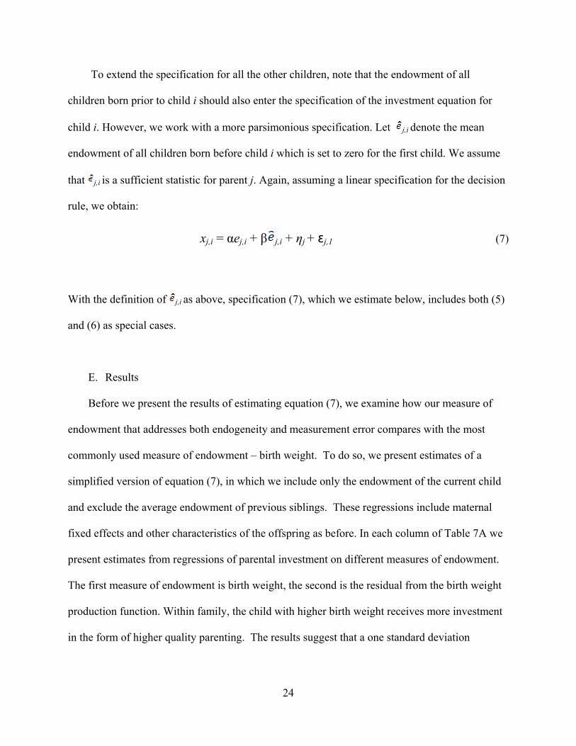
To extend the specification for all the other children, note that the endowment of all

children born prior to child i should also enter the specification of the investment equation for

child i. However, we work with a more parsimonious specification. Let j,i denote the mean

endowment of all children born before child i which is set to zero for the first child. We assume

that j,i is a sufficient statistic for parent j. Again, assuming a linear specification for the decision

rule, we obtain:

xj,i = αej,i + β j,i + ηj + ɛj,1 (7)

With the definition of j,i as above, specification (7), which we estimate below, includes both (5)

and (6) as special cases.

E. Results

Before we present the results of estimating equation (7), we examine how our measure of

endowment that addresses both endogeneity and measurement error compares with the most

commonly used measure of endowment – birth weight. To do so, we present estimates of a

simplified version of equation (7), in which we include only the endowment of the current child

and exclude the average endowment of previous siblings. These regressions include maternal

fixed effects and other characteristics of the offspring as before. In each column of Table 7A we

present estimates from regressions of parental investment on different measures of endowment.

The first measure of endowment is birth weight, the second is the residual from the birth weight

production function. Within family, the child with higher birth weight receives more investment

in the form of higher quality parenting. The results suggest that a one standard deviation

25

difference in birth weight between siblings can explain ten percent of the average difference in

investment between siblings within families.

When we consider that birth weight may be endogenous because it already reflects maternal

prenatal investments and use instead the residual from a birth weight production function which

includes maternal smoking, pre-pregnancy weight and weight gain as regressors (results are

presented in Tables 5 and 6) we find that the relationship still holds, though it is slightly

attenuated. In columns 3-8 we present estimates based on different measures of health at birth

(gestation, body length, head circumference) and their corresponding “residual” measures and

the same pattern emerges. In the last two columns we present estimates for a measure of

endowment based on factor scores of multiple measures of health at birth (birth weight, head

circumference, body length, gestation), and factor scores based on the four residuals from the

newborn health production function. The results based on factor scores of the four measures of

health at birth (column 9) are similar though slightly smaller than the birth weight result in

column 1 and the results based on factor scores of the four residuals is still positive and

significant, but only 40 percent of the original estimate based on birth weight and presented in

column 1.

We estimate equation (7) substituting different measures of endowments and present the

results in Table 7B. We find that the focal child’s endowment relative to the endowment of

siblings born prior to him has a positive impact on investment in that child. In other words, the

lower the focal child’s endowment relative to previously born siblings, the greater the investment

in that child. We interpret this as evidence of compensating investment and consistent with

parental preference for equality among siblings. However, conditional on this, we find that

parents will invest more in children with higher initial endowments, consistent with incentives

26

generated by the greater return to investments in more highly endowed children. We repeat this

for multiple measures of endowment (columns 2-4), as well as the factor scores (column 5) and

find the same pattern.

We follow this with an exploration of whether investment behavior (specifically, how it

responds to endowment) varies with parental resources and fertility. To do so, we estimate the

ability of initial endowment to predict future human capital (7 year IQ) within family, stratified

by parental resources and fertility. We find that within family, the relationship between initial

endowments and later human capital is stronger for families with fewer resources as proxied by

maternal education and family income at birth, (Table 8A). This is true for each of the four

measures of initial endowment that we use (birth weight, residual birth weight, factor scores of

four measures of health at birth, and factor scores based on the residual measures). We interpret

this as evidence of greater reinforcing investments among families with fewer resources. If

investment had been compensating, we would have seen more convergence in human capital at

age 7. We find a similar pattern by fertility, which is not surprising, given that fertility and

income are negatively correlated. Reinforcing investments are more common in larger families,

as measured by multiple measures of endowment (Table 8B).

This heterogeneity is consistent with existing empirical evidence showing patterns of

compensating investments in a rich country such as Norway (Black, Devereaux and Salvanes,

forthcoming) and reinforcing investments in a poor country such as China (Rozenzweig and

Zhang, 2010). It is also consistent with the findings of Hsin (2009) who finds that higher income

parents invest in a compensatory way, while lower income parents invest in a more reinforcing

manner using the PSID. However, these findings are inconsistent with models of parental

investments developed by Becker and Tomes (1986) which stipulate that parents care about

27

equality of consumption among their adult children and that parents with greater resources are

more likely to invest in a reinforcing manner because they can offset inequality of human capital

through compensating bequests. In contrast, parents with fewer resources who care about

equality among their children are more likely to invest in a compensating manner.

In the next section, we develop an alternative model of parental investments that maintains

many of the features of the previous model (complementarity of initial human capital and

investments in the production of later human capital, parental preference for equality of

consumption among siblings) but that incorporates the concept of altruism among siblings. Our

model allows for parents with fewer resources to invest in a reinforcing manner because they can

also invest in sibling altruism whereby adult offspring with greater human capital will make

transfers to their siblings with lower levels of human capital. We follow this with the

presentation of evidence on sibling altruism from the PSID that is consistent with this.

IV. A Model of Quantity-Quality Interaction with Heterogeneous Children

Following Becker and Lewis (1973), we consider a model in which parents choose how

many children to have and how much to invest in each child. Unlike Becker and Lewis, children

are heterogeneous with respect to their endowments. As in Behrman, Pollak, and Taubman

(1982), parents are averse to inequality across children. Heterogeneity, inequality aversion,

parental resources, and a constraint preventing parents from borrowing against future resources

of their children are the features that influence parental choices of quality and quantity of

children. This model is consistent with the following findings in the literature: 1) a negative

estimated income inequality of fertility, 2) a positive income elasticity of quality, 3) reinforcing

28

investments and 4) that investments and child quality may decrease as the number of children

increase.

This model also predicts that investments will become more reinforcing as family size

increases. This is due to the fact that families with less income have more children and are more

likely to be affected by the constraint that they can't borrow against the future income of

children. As a result, parents in poor and large families face an equity-efficiency trade-off. On

the one hand, the production function dictates investments be made in the children with higher

endowment. On the other hand, parental aversion to inequality dictates investments be made in

the children with lower endowment. This existing model predicts that as family size increases,

the latter effect becomes stronger, so according to the model, investments become less

reinforcing as family size increases.

This is in fact not what we find in our data. Nor is it consistent with existing empirical evidence

mentioned previously. As a result, we extend the above model by allowing parents to mould the

preferences of their children. In particular, we focus on the case in which parents spend resources

so that children are altruistic toward each other. We show that altruism breaks the efficiency-

equity trade-off: parents invest in the most promising children, who have much higher quality

than their siblings with lower endowment, but due to altruism among sibling, the high-quality

children transfer resources to siblings with lower quality, enabling equality of consumption

among siblings.

Timing

29

In our model, the parents live for two periods. In the first period, they choose how many

children to have. In the second period, children are born, parents observe the realized

endowment, and choose how much to invest in the quality of their children as well as the amount

of financial wealth to bequeath. Children also live for two periods. In the first period, they reside

with their parents and receive investments in their quality. In the second period, they receive any

financial bequests left by the parents. The children work and are paid according to their quality.

Finally, they choose how to allocate resources across siblings, they consume the resources

allocated to them, and they die.

Fertility

At the moment that parents make fertility choices, they know present value of their resources,

. All of the children are born at the beginning of the second period. From the point of view of

the parent making fertility choices, the endowments of the children are stochastic. We assume

that these endowments are identically distributed, but correlated across children within a family.

Let be the vector of endowments. We denote by the period two

utility of the parent. Let , , denote unobserved components that affect fertility

choices. Let denote the expected lifetime utility of having children:

30

The number of children chosen by the parent is:

Investments in Quality and Financial Bequests

Once children are born, parents observe the realization of the endowment vector and they

choose how much resources to spend on the production of child quality. This requires the

purchase of two types of goods. This first are goods shared among all chidlren in the household,

, and which can be thought as the quality of the housing or the neighborhood where the family

lives. The second good , is child specific and includes, for example, the number of hours a

given child spends with a tutor. The quality of child , , is produced according to function by

combining the child's endowment with common inputs , and specific inputs :

(8)

31

We assume that quality where is increasing, concave, and twice differentiable. We assume that

quality is measured in dollars.

We denote by and the prices of goods and , respectively. The parent chooses how much to

consume, , and how much to bequeath in financial wealth to child , . The interest rate is .

We denote by the cost of raising a child with quality zero, measured in units of parental

consumption. The budget constraint facing the parent is:

(9)

In the classic quantity-quality interaction model, for all so . In our case,

investments differ across children in the same household because each child has a different

endowment. We impose the restriction that parents cannot leave debts to the children, so:

(10)

Parents invest in the quality of their children for two reasons. First, both the quantity and the

quality of children affect the parental utility directly. We follow Behrman, Pollak, and Taubman

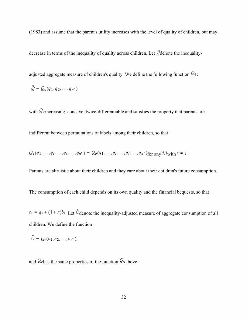
32

(1983) and assume that the parent's utility increases with the level of quality of children, but may

decrease in terms of the inequality of quality across children. Let denote the inequality-

adjusted aggregate measure of children's quality. We define the following function :

with increasing, concave, twice-differentiable and satisfies the property that parents are

indifferent between permutations of labels among their children, so that

for any with

Parents are altruistic about their children and they care about their children's future consumption.

The consumption of each child depends on its own quality and the financial bequests, so that

. Let denote the inequality-adjusted measure of aggregate consumption of all

children. We define the function

and has the same properties of the function above.

33

Let denote the value function of the parent that has state vector . The

problem of the parent is to choose common investments child-specific investments

, and bequests that solves

(11)

subject to (8), (9), and (10).

First-order conditions

We start by analyzing the first-order conditions for families in which siblings are selfish, so that

. In this case, the Euler equation for investment inputs and is:

(12)

The Euler equation shows that the larger the higher the demand for the common good ,

34

because raises the quality of all children in the household, while raises the quality of only

child

We differentiate our analysis for two types of families, "rich" and "poor". We denote "rich" the

families for which the restriction (10) does not bind and "poor" the families for which (10) does

bind. For rich families, it is easy to show that investments in the quality of children satisfy the

following Euler equation:

(13)

It is also possible to show that bequests for any two children in the household, whenever

positive, satisfy the relationship:

so that if , then Note, however, that whether investments reinforce or

compensate endowments depends on how much parents dislike inequality in quality, as

measured by the function , the concavity of the production function , and the degree of

complementarity between and in the production of quality. For rich families, the function ,

that describes how parents discount inequality in consumption, does not play an important role

because rich parents equate consumption of children via bequests.

35

For poor families, both the function and the elasticity of substitution between and

play a role. To see how the latter influences parental investments, consider two families, A and

B, that are equal in terms of parental income and number of children, but their children are

different in the sense that the endowment of children in family , is higher then

the endowment of children in family . For simplicity, we are assuming that

all children in the same family have exactly the same endowment, so there is no heterogeneity

within family. Will investments be higher in family or in family ? On the one hand, the

higher productivity of investments in family A children induces a substitution effect away from

parental consumption and towards higher investments in quality of children in family .

However, because endowments in family are already higher than in family , that means that

higher investments in family would make the quality of children in family much higher than

the quality of children in family . This implies that the consumption of children in family will

be higher than the consumption of children in family . Because families have the same income,

this implies that the parental consumption in family would be lower than the parental

36

consumption in family . The higher marginal utility of parental consumption induces an income

effect that drives resources away from investments in children and towards higher parental

consumption in family . The income effect dominates the substitution effect the lower the

elasticity of substitution between parental consumption and .

To see the role that plays, assume now that there is heterogeneity across children in

terms of their endowments. Suppose that the first child has high endowment and that the last

child has the low endowment. By devoting more resources to the first rather than the last child,

the parents are reinforcing initial differences and making their consumption unequal. Because

there is a trade-off between level and inequality of consumption across children, poor parents

may invest in a compensating manner if their inequality aversion is high.

However, what we observe in the data is the opposite: that reinforcing behavior is greater in

large families and in poor families (Tables 8A and 8B), which, as noted previously, is also

consistent with patterns observed in rich vs poor countries and for rich and poor families in the

US.

Altruism Among Siblings

We now propose an extension that can explain why parental investments become more

reinforcing the larger the family size is. As explained above, poor parents face an equity-

37

efficiency trade-off and this implies that investments in poor and large families should not

become more reinforcing.

If siblings were altruistic towards each other, and if they could act on that altruism, then it

would be possible for parents to invest more in the children with the higher endowments. The

siblings would then transfer resources to the children that have the lowest endowments. This

would then break the equity-efficiency trade-off that parents in poor and large families face.

However, a necessary condition for this to happen is that parents have to care more about

inequality in consumption than inequality in quality, because the former is transferable across

children, while the latter is not.

We consider an extension of the model in which parents can invest in sibling altruism. We

denote by the price of the investment in altruism among siblings, . The budget

constraint becomes:

(14)

We next derive the consumption of children when we allow parents to invest in altruism among

siblings, which we denote by . As before, is the consumption of child . The lifetime

utility of child is:

38

(15)

The larger , the more altruism children have towards siblings. In the case when , then

and each child values her siblings' consumption just as much as her

own consumption. Note that we assume that the children's preferences with respect to

consumption is represented by the natural logarithm utility function. While this logarithm

assumption is clearly restrictive, it will be convenient for our framework.

The fact that children are altruistic towards each other requires us to describe the way children

decide how to allocate consumption. We assume that children choose collectively as in

Chiappori (1988). The collective framework assumes that choices are Pareto optimal. To focus

on the importance of altruism, we assume that the Pareto weight of child is . We

write the objective function of the children as:

(16)

Children pool resources. Let , where The budget constraint facing

children is then Under this framework, it is easy to show that the consumption of

39

child is given by:

(17)

which shows that children's consumption depend not only on their resources, but also on the

pooled resources of their siblings. In the case when altruism is perfect, so that , then there

is perfect sharing: for all When , so that there is no altruism across siblings, then

which means that the consumption of a child depends only on her own resources.

The parental problem is to maximize (11) subject to the budget constraint (14), the production

function of human capital (7), the non-negativity constraints for bequests (10), the consumption

function (), and the constraint that . It is particularly interesting to derive the first-order

conditions for bequests and altruism . Let and denote the Kuhn-Tucker multipliers

associated with the restrictions () and , respectively. Then:

(18)

At the optimal, bequests are such that they equalize the marginal utility of parental consumption

40

to the marginal utility of inequality-adjusted aggregate consumption of children. Note that by

increasing bequests to child by a small amount, the parent not only increases the consumption of

child , but the parent potentially increases the consumption of all the other children as well. This

only occurs, however, if children are altruistic, so that . The first-order condition for

investments in altruism are:

The following proposition states that if parents are rich enough that they make financial transfers

to children, then they don't invest in altruism across children.

Proposition:

Assume that satisfies equal concern, is increasing, and strictly concave. Assume that .

If for all , the .

Proof:

41

Suppose that for all . Then, from the first-order conditions for and we obtain the

following equality:

But if for any :

It then follows that . Using these facts in the summation term in the right-hand side of

the first-order condition for altruism, we obtain:

which implies that

Altruism is a way for poor parents who cannot make financial bequests to break the efficiency-

equity trade-off. Rich families do not face such trade-off because they have resources to invest

optimally in the human capital of their children. Another way to re-state the proposition is that if

42

then . Families that invest in altruism are not rich enough to transfer financial

bequests to children and altruism among siblings allow parents to overcome the equity-efficiency

trade-off.

Empirical Evidence in Favor of Sibling Altruism

The PSID asks individuals in 1988 whether they gave any monetary help to relatives, and if so,

who are the relatives to whom they gave these transfers. Most of the transfers reported by the

PSID respondents are to the respondent's children or respondent's parents. A very small fraction,

2.6% , of respondents inform report they gave some money to siblings. For those who report a

positive transfer to a sibling, the mean value is $670, the median value is U$300, the 10th

percentile is U$100, and the 90th percentile is $1800. We run a tobit regression of log monetary

help against a dummy variable for growing up in a poor family, dummy variables for number of

siblings, natural log of average income from 1985 to 1989, and dummies for race and gender.

We find that among siblings, those who grew up in poor families transferred more money to their

siblings, consistent with the model (Table 9).

V. Conclusion

In this paper we examine the factors influencing the production of human capital during

childhood. Our paper makes a number of important contributions. First, we provide empirical

evidence regarding the mechanics of the production function, namely that the two primary inputs

(initial human capital and investments) are complements in the production of human capital.

While many of the existing models of human capital production assume this complementarity,

43

the empirical evidence, to this point, has been weak. Our finding that the impact of preschool is

greatest for the most highly developed infants, represents a contribution because it is based on a

plausibly exogenous source of variation in investment which is needed for identification: the

launch of Head Start in 1966. It also contributes to the growing literature on the impact of Head

Start and other high quality preschool programs.

Our second contribution is our use of alternative measures of endowments and investments

to estimate whether parents invest in a reinforcing or compensatory manner. Moreover, we

extend this analysis to consider heterogeneity in the investment decision. We find that parents

with fewer resources who, according to existing theory, should be most likely to invest in a

compensatory way because they are unable to make offsetting financial bequests, are in fact

more likely to invest in a reinforcing way. Though this is inconsistent with existing theory, it is

consistent with existing empirical work on this topic. Thus we develop a model of parental

investments, child heterogeneity in endowments and fertility that departs from existing models

with the introduction of the concept of sibling altruism. By allowing poor families to invest in

sibling altruism whereby adult offspring with the highest levels of human capital can transfer

resources to siblings with less human capital, poor families who care about equality of

consumption among their children are not limited to compensatory investments. Rather, with

sibling altruism, poor parents can invest more efficiently by investing in their children with

higher initial human capital, thereby increasing the return on their investments, without

sacrificing equality. This model creates a coherent framework that can explain much of the

emerging empirical literature on the interaction between parental investments and child

endowments.

44

45

References - INCOMPLETE

Ananat, Elisabeth and Daniel Hungerman. The power of the Pill for the Marginal Child: Oral Contraception’s Effects on Fertility, Abortion, and Maternal and Child Characteristics. Unpublished mimeo, Duke University.

Angrist, Joshua, Lavy, Victor and Analia Schlosser, “New Evidence on the Causal Link

Between the Quantity and Quality of Children.” NBER WP # 11838, 2005. Ashenfelter, Orley and Cecilia Rouse. Income, schooling, and ability: Evidence from a new

sample of identical twins. Quarterly Journal of Economics, 113(1):253–284, 1998. Almond, Douglas and Janet Currie. Human Capital Development Before Age Five. NBER

WP # 15827, March 2010. Becker, Gary. 1981. A Treatise on the Family. Cambridge, MA: Harvard University Press. Becker, Gary and Nigel Tomes. Child endowments and the quantity and quality of children.

The Journal of Political Economy, 84(4):S143–S162, August 1986. Becker, Gary and Gregg Lewis. On the Interaction between the Quantity and Quality of

children. Journal of Political Economy. LXXXI: S279-S288, 1973. Behrman, Jere, Pollak, Robert, and Paul Taubman. Parental preferences and provision for

Progeny. Journal of Political Economy, 90(1):52–73, 1982. Behrman, Jere, Rosenzweig, Mark and Paul Taubman. Endowments and the allocation of

schooling in the family and in the marriage market: The twins experiment. Journal of Political Economy, 102(6):1131–1174, 1994.

Black, Sandra, Devereaux, Paul and Kjell Salvanes. The More the Merrier? The Effect of

Family Size and Birth Order on Children’s Education. The Quarterly Journal of Economics, 2005.

Black, Sandra, Devereaux, Paul and Kjell Salvanes. Small Family, Smart Family? Family

Size and the IQ Scores of Young Men, (NBER Working Paper #13336, August 2007), Journal of Human Resources, forthcoming.

Bradley, Robert, Corwyn, Robert, McAdoo, Hariett and Cynthia Garcia Coll. “The Home

Environments of Children in the US Part I: Variations by Age, Ethnicity, and Poverty Status.” Child Development. 72(6):1844, 1867, 2001.

Cunha, Flavio and James Heckman. The technology of skill formation. American Economic

Review, 97(2):31–47, May 2007.

46

Currie, Janet and Duncan Thomas. Does head start make a difference? American Economic Review, 85(3):341–364, 1995.

Currie, Janet and Duncan Thomas. Early test scores, socioeconomic status and future

outcomes. NBER WP# 6943, 1999. Garces, Eliana Duncan Thomas, and Janet Currie. Longer-term effects of head start.

American Economic Review, 92(4):999–1012, September 2002. Hanushedk, Eric. The Trade-Off Between Child Quantity and Quality. Journal of Political

Economy. 84-117, 1992. Heckman, James J. Lessons from The Bell Curve. Journal of Political Economy,

103(5):1091, 1995. Heckman, James, Malofeeva, Lena, Pinto, Rodrigo and Peter Savelyev. Understanding the

Mechanisms Through Which an Influential Early Childhood Program Boosted Adult Outcomes. Mimeo University of Chicago, 2010.

Hopkins, Kenneth D. and Glenn H. Bracht. Ten-Year Stability of Verbal and Nonverbal IQ

Scores. American Educational Research Journal, 12(4):469–477, 1975. Hsin, Amy. Is Biology Destiny? Birth Weight and Differential Parental Treatment.

Unpublished manuscript, Populations Studies Center, University of Michigan, 2009. Lazarus, RS. On the Primacy of Cognition. American Psychologist. 39:124-129, 1984. Ludwig, Jens and Douglas L. Miller. Does head start improve children’s life chances?

evidence from a regression discontinuity design. Quarterly Journal of Economics, 488(1):159–208, February 2007.

McLeod, Jane and Karen Kaiser. Childhood emotional and behavioral problems and

educational attainment. American Sociological Review, 69(5):636–658, 2004. Murnane, Richard J., John B. Willett, and Frank Levy. The Growing Importance of

Cognitive Skills in Wage Determination. Review of Economics and Statistics, 77(2):251–266, 1995.

O’Connor, Thomas G., Michael Rutter, Celia Beckett, Lisa Keaveney, Jana M. Kreppner,

and the English and Romanian Adoptees Study Team. The Effects of Global Severe Privation on Cognitive Competence: Extension and Longitudinal Follow-Up. Child Development,71(2):376–390, 2000.

Paxson, Christina and Norbert Schady “Cognitive Development Among Young Chidlren in

Ecuador: the Roles of Wealth, Health and Parenting.” Journal of Human Resources, XLII(1):49-84, 2007.

47

Pitt, Mark, Rosenzweig, Mark and Nazmul Hassan. Productivity, health, and inequality in the intrahousehold distribution of food in low-income countries. American Economic Review, 80(5):1139–1156, December 1990.

Ranson, Kenna and Liana Urichuk. “The Effect of Parent-Child Attachment Relationships

on Child Biopsychosocial Outcomes: A Review.” Early Child Development and Care. Vol 178(2): 129-152, 2008.

Rosenzweig, Mark and Kenneth Wolpin. Testing the Quantity-Quality Fertility Model: the

Use of Twins as a natural Experiment. Econometrica XLVIII: 227-240, 1980. Rosenzweig, Mark and Junsen Zhang . Do Population Control Policies Induce More Human

Capital Investment? Twins, Birth Weight and China's "One-Child" Policy. Review of Economic Studies. 76(3) :1149-1174, 2009.

Schore, Allan. “Effects of a Secure Attachment Relationship on Right Brain Development,

Affect Regulation and Infant Mental Health.” Infant Mental Health Journal, vol 22(1-2):7-66, 2001.

Suitor, Jill, Sechrist, Jori, Mikuhn, Mari, Pardo, Seth and Karl Pilemer. Within-Family

Differences in Parent-Child Relations Across the Life Course. Current Directions in Psychological Sciences. 17:334-338, 2008.

Panel A: Full Sample1963‐1964 1965 1966 1967 1968 1969 1970

Local HS spending per poor person in 1968 0.000309 0.0006 0.00452 0.00308 0.00361 0.00157 0.00132[0.000982] [0.00113] [0.00180] [0.00177] [0.00224] [0.00185] [0.00175]

Observations 6122 5099 5442 5571 6178 5616 1627R‐squared 0.012 0.021 0.021 0.019 0.017 0.034 0.048Robust standard errors in brackets

Panel B: Limiting to Mothers with no More than a High School Degree1963‐1964 1965 1966 1967 1968 1969 1970

Local HS spending per poor person in 1968 0.000158 0.000692 0.00525 0.00392 0.0044 0.00342 0.00463[0.000754] [0.00102] [0.00176] [0.00162] [0.00187] [0.00162] [0.00169]

Observations 5637 4642 4875 4990 5538 4872 1308R‐squared 0.008 0.013 0.023 0.022 0.016 0.022 0.047

Panel C: Include Mother FEALL <=HS

Local HS Spending (=0 in years prior to 1966) 0.00183 0.00251[0.000978] [0.00101]

ObservationsR‐squared 0.894 0.882Robust standard errors in brackets 12938 11670

OLS regressions in planels A and B include controls for offspring gender, birth order dummies, maternal race, maternal education,materal age, marital status and family income at birthFE Regressions in panel C include controls for gender, birth order, maternal age, marital status, family income at birth and a quadratic in year of birth

Local (county) Head Start spending per poor person in 1968 ranges from $3 to $29

Table 1: Correlation between Local Head Start Spending Per Poor Person 1968 and Preschool Enrollment

Panel A: OLS Regressions (1) (2) (3) (4) (5) (6) (7)Birth Weight ‐ Standardized ‐0.00247 ‐0.00297

[0.00402] [0.00419]Low Birth Weight 0.00111

[0.0107]Weeks of Gestation at Birth ‐0.00094

[0.00112]Premature birth 0.0151

[0.0113]8 Month Mental Bayley ‐ Standardized 0.000834 0.00384 0.00158

[0.00354] [0.00448] [0.00369]8 Month Motor Bayley ‐ Standardized ‐0.00517

[0.00423]Maternal Education at Birth 0.00392 0.00391 0.00386 0.00387 0.00391 0.00391 0.00392

[0.000820] [0.000820] [0.000819] [0.000819] [0.000819] [0.000819] [0.000820]Maternal Age at Birth 0.000277 0.00027 0.000236 0.00026 0.00024 0.000245 0.00027

[0.000762] [0.000762] [0.000762] [0.000762] [0.000761] [0.000762] [0.000762]Family income (real) at pregnancy in $1000 0.000216 0.000212 0.000203 0.000202 0.000211 0.000204 0.000216

[0.000286] [0.000286] [0.000286] [0.000286] [0.000286] [0.000286] [0.000286]Married ‐0.00713 ‐0.00722 ‐0.00859 ‐0.00848 ‐0.00754 ‐0.0073 ‐0.0071

[0.00987] [0.00987] [0.00987] [0.00987] [0.00985] [0.00986] [0.00987]Black 0.0208 0.0208 0.0197 0.0196 0.0202 0.0211 0.0207

[0.0479] [0.0479] [0.0478] [0.0478] [0.0478] [0.0478] [0.0479]White ‐0.102 ‐0.102 ‐0.103 ‐0.103 ‐0.103 ‐0.103 ‐0.102

[0.0472] [0.0472] [0.0472] [0.0472] [0.0472] [0.0472] [0.0472]Hispanic ‐0.0611 ‐0.0614 ‐0.0617 ‐0.0618 ‐0.0616 ‐0.0613 ‐0.0611

[0.0543] [0.0543] [0.0542] [0.0542] [0.0542] [0.0542] [0.0543]Male ‐0.013 ‐0.0134 ‐0.0135 ‐0.0134 ‐0.0134 ‐0.0136 ‐0.0129

[0.00662] [0.00659] [0.00658] [0.00658] [0.00657] [0.00658] [0.00663]First born 0.0373 0.0377 0.0369 0.037 0.0373 0.0391 0.0368

[0.0132] [0.0132] [0.0132] [0.0132] [0.0132] [0.0132] [0.0132]Second Birth 0.0349 0.0352 0.0348 0.035 0.0349 0.0355 0.0347

[0.0112] [0.0112] [0.0112] [0.0112] [0.0112] [0.0112] [0.0112]Third or Fourth Birth 0.0112 0.0114 0.0105 0.0107 0.0112 0.0114 0.0111

[0.00958] [0.00957] [0.00957] [0.00958] [0.00957] [0.00957] [0.00958]

Observations 10156 10156 10132 10132 10167 10160 10156R‐squared 0.047 0.047 0.048 0.048 0.047 0.047 0.047

Panel B: Maternal FE RegressionsBirth Weight ‐ Standardized 0.00039 0.00151

[0.00857] [0.00880]Low Birth Weight ‐0.00928

[0.0191]Weeks of Gestation at Birth ‐0.00209

[0.00190]Premature birth 0.00789

[0.0187]8 Month Motor Bayley ‐ Standardized ‐0.00298

[0.00680]8 Month Mental Bayley ‐ Standardized ‐0.00309 ‐0.00147 ‐0.00327

[0.00569] [0.00679] [0.00584]Observations 10157 10157 10133 10133 10168 10161 10157R‐squared 0.739 0.739 0.739 0.739 0.738 0.738 0.739

Standard errors in bracketsAMC FE and year of birth indicators included in top panelMaternal FE and year of birth indicators included in bottom panel

Table 2 Determinants of Investment Across Families: Dependent Variable= Preschool

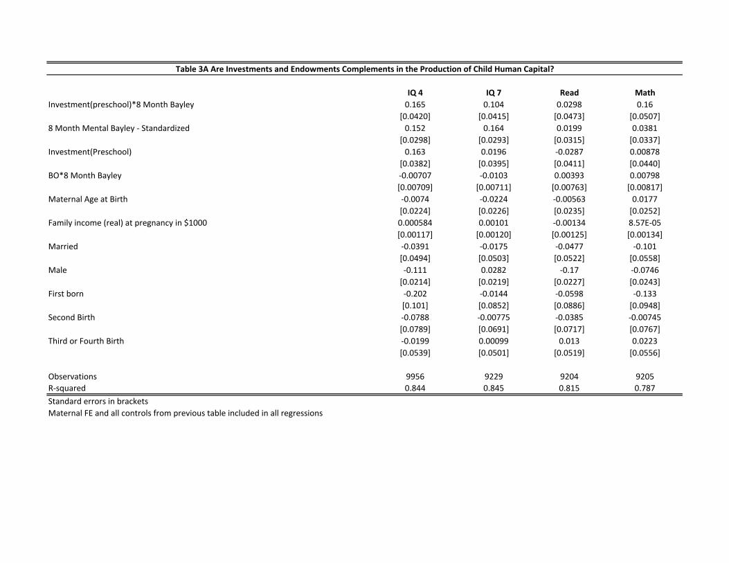
IQ 4 IQ 7 Read MathInvestment(preschool)*8 Month Bayley 0.165 0.104 0.0298 0.16

[0.0420] [0.0415] [0.0473] [0.0507]8 Month Mental Bayley ‐ Standardized 0.152 0.164 0.0199 0.0381

[0.0298] [0.0293] [0.0315] [0.0337]Investment(Preschool) 0.163 0.0196 ‐0.0287 0.00878

[0.0382] [0.0395] [0.0411] [0.0440]BO*8 Month Bayley ‐0.00707 ‐0.0103 0.00393 0.00798

[0.00709] [0.00711] [0.00763] [0.00817]Maternal Age at Birth ‐0.0074 ‐0.0224 ‐0.00563 0.0177

[0.0224] [0.0226] [0.0235] [0.0252]Family income (real) at pregnancy in $1000 0.000584 0.00101 ‐0.00134 8.57E‐05

[0.00117] [0.00120] [0.00125] [0.00134]Married ‐0.0391 ‐0.0175 ‐0.0477 ‐0.101

[0.0494] [0.0503] [0.0522] [0.0558]Male ‐0.111 0.0282 ‐0.17 ‐0.0746

[0.0214] [0.0219] [0.0227] [0.0243]First born ‐0.202 ‐0.0144 ‐0.0598 ‐0.133

[0.101] [0.0852] [0.0886] [0.0948]Second Birth ‐0.0788 ‐0.00775 ‐0.0385 ‐0.00745

[0.0789] [0.0691] [0.0717] [0.0767]Third or Fourth Birth ‐0.0199 0.00099 0.013 0.0223

[0.0539] [0.0501] [0.0519] [0.0556]

Observations 9956 9229 9204 9205R‐squared 0.844 0.845 0.815 0.787

Standard errors in bracketsMaternal FE and all controls from previous table included in all regressions

Table 3A Are Investments and Endowments Complements in the Production of Child Human Capital?

OLS FE OLS FE OLS FE OLS FE OLS FE OLS FE OLS FEPreschool   0.193 0.01 0.197 0.0102 0.221 ‐0.0476 0.182 ‐0.00642 0.19 0.0223 0.00722 ‐0.112 0.0596 ‐0.0265

[0.0257] [0.0393] [0.0256] [0.0391] [0.0492] [0.0770] [0.0353] [0.0498] [0.0251] [0.0388] [0.0925] [0.121] [0.109] [0.152]Preschool*bw ‐0.0331 ‐0.00195 ‐0.0406 ‐0.0361

[0.0303] [0.0455] [0.0315] [0.0476]Preschool*BO ‐0.0107 0.0158 ‐0.0161 0.0174

[0.0132] [0.0192] [0.0128] [0.0189]Preschool*male 0.0217 0.0366 0.0209 0.0465

[0.0502] [0.0681] [0.0496] [0.0683]Preschool*8 Month Bayley 0.0679 0.108 0.0447 0.114

[0.0301] [0.0408] [0.0347] [0.0484]Preschool*advanced social/emotional development 0.65 0.614 0.648 0.403

[0.261] [0.329] [0.265] [0.337]Preschool*normal social/emotional development 0.195 0.127 0.18 ‐0.0392

[0.0960] [0.125] [0.104] [0.142]

Birth Weight ‐ Standardized 0.127 0.146 0.0758 0.113[0.0109] [0.0211] [0.0113] [0.0218]

8 Month Mental Bayley ‐ Standardized 0.186 0.127 0.168 0.121[0.00959] [0.0148] [0.0111] [0.0167]

Advanced Social/Emotional Development 0.491 0.233 0.0926 0.017[0.0758] [0.0997] [0.0781] [0.102]

Normal Social/Emotional Development 0.265 0.0989 0.00523 ‐0.045[0.0324] [0.0446] [0.0353] [0.0476]

Observations 9339 9340 9330 9331 9228 9229 9339 9340 9339 9340 9325 9326 9205 9206R‐squared 0.289 0.839 0.3 0.842 0.289 0.84 0.289 0.839 0.322 0.844 0.298 0.84 0.327 0.848

Standard errors in bracketsRegressions include controls listed previouslyALL OLS regressions include controls for maternal characteristics (education, age, race, family income), offspring characteristics (birth order, gender, year of birth and AMC indicators.)ALL FE regressions include controls for maternal age, family income, birth order, gender and year of birth indicatorsNote: only 208 observations with advanced social/emotional development at 8 months of age.

Table 3B Heterogeneity in Impact of Preschool on 7 Year IQ

Factor analysis/correlation   Number of obs    =    31538   Method: principal factors Retained factors =        3Rotation: (unrotated)     Number of params =       18

   Factor   Eigenvalue   Difference Proportion  Cumulative    Factor1  1.43651 1.298 1.2976 1.2976   Factor2  0.13851 0.10684 0.1251 1.4227   Factor3  0.03167 0.04018 0.0286 1.4513   Factor4  ‐0.00851 0.08304 ‐0.0077 1.4437   Factor5  ‐0.09155 0.08883 ‐0.0827 1.361   Factor6  ‐0.18038 0.03883 ‐0.1629 1.198   Factor7  ‐0.21921 ‐0.198 1 LR test: independent vs. saturated:  chi2(28) = 2.9e+04 Prob>chi2 = 0.0000  

Factor loadings (pattern matrix) and unique variances   

  Variable  Factor1  Factor2   Factor3   Uniqueness  Appearance of Child 0.1751 0.1166 0.1212 0.9411Responsivenes of Mother 0.5889 0.1525 ‐0.0017 0.63Affection 0.6213 ‐0.1497 0.0097 0.5915Focus on child 0.4744 ‐0.2363 0.0007 0.7191Management of Child 0.3324 0.0991 ‐0.0451 0.8776Attention to Child 0.3056 0.096 ‐0.1127 0.8847Handling of Child 0.4941 0.066 0.0463 0.7493

Scoring coefficients (method = regression)    

Variable   Factor1   Factor2  Factor3 Appearance of Child 0.06217 0.10178 0.12009Responsivenes of Mother 0.28604 0.18732 ‐0.00392Affection 0.31456 ‐0.18048 0.01248Focus on child 0.19967 ‐0.24249 ‐0.00068Management of Child 0.12527 0.09371 ‐0.04763Attention to Child 0.11425 0.08734 ‐0.11782Handling of Child 0.20764 0.07053 0.05466

Table 4 Development of Measure of Parental Investment: Factor Analysis

(1) (2) (3) (4)

Standardized Birthweight

Standardized Head Circumference at Birth

Standardized Body Length

Standardized Gestation Length

Number of Cigarretes Smoked ‐0.0114 ‐0.00998 0.0423 0.0612[0.0361] [0.0462] [0.0528] [0.0197]

Pre pregnancy weight 0.0202 0.0192 0.0207 0.00569[0.00130] [0.00168] [0.00192] [0.000712]

Weight gain during pregnancy 0.0292 0.0271 0.0281 0.0084[0.00138] [0.00179] [0.00205] [0.000756]

Maternal Age at Birth ‐0.0695 ‐0.0582 ‐0.0902 ‐0.0361[0.0156] [0.0201] [0.0229] [0.00854]

Family income (real) at pregnancy in $1000 ‐6.39E‐05 0.000528 0.000513 ‐5.67E‐05[0.000798] [0.00103] [0.00117] [0.000437]

Married ‐0.0799 ‐0.0241 ‐0.0617 ‐0.0118[0.0328] [0.0422] [0.0481] [0.0180]

Male 0.176 0.345 0.253 ‐0.0216[0.0150] [0.0193] [0.0221] [0.00821]

First born ‐0.122 ‐0.0158 0.0719 ‐0.00821[0.0535] [0.0686] [0.0785] [0.0293]

Second Birth ‐0.0321 0.0334 0.0612 ‐0.0354[0.0433] [0.0555] [0.0635] [0.0237]

Third or Fourth Birth ‐0.0144 0.025 0.0123 ‐0.0185[0.0313] [0.0402] [0.0459] [0.0172]

Observations 11373 11290 11248 11345R‐squared 0.852 0.82 0.777 0.743

Standard errors in bracketsAlso included as covariates are maternal fixed effects and indicators for year of birth

Table 5: Estimating Endowments

Variable Factor LoadingsVariance of Uniqueness

Fraction of Total Variance 

Explained by the Factor

Standardized Birth Weight 0.899 0.192 0.813Standardized Head Circumference at Birth 0.823 0.323 0.704Standardized Body Length at Birth 0.805 0.352 0.681Standardized Weeks of Gestation 0.466 0.782 0.357

Factor EigenvalueFactor1 2.350Factor2 ‐0.026Factor3 ‐0.050Factor4 ‐0.129

VariableScoring 

CoefficientsStandardized Birth Weight 0.486Standardized Head Circumference at Birth 0.260Standardized Body Length at Birth 0.233Standardized Weeks of Gestation 0.071

Number of Observations 13147

Table 6: Factor Loadings and Variances of Uniqueness

Determining the Number of Factors

Factor Scoring by the Regression Method

(1) (2) (3) (4) (5) (6) (7) (8) (9) (10)Birth Weight ‐ Standardized 0.0618

[0.0191]BW Residual Endowment 0.0592

[0.0219]Gestation ‐ Standardized 0.043

[0.0128]Gestation Residual Endowment 0.0355

[0.0140]Body Length ‐ Standardized 0.0234

[0.0138]Body Length Residual Endowment 0.0268

[0.0152]Head Circumference ‐ Standardized 0.0277

[0.0155]Head Circumference Residual Endowment 0.0272

[0.0172]Factor Scores of BW, gestation, body length, and head circumference 0.05

[0.0174]Factor Scores from residuals of BW, gestation, body length, and head circumferen 0.0203

[0.00791]

Observations 12611 11598 12582 11568 12469 11473 12515 11515 12420 11425R‐squared 0.664 0.676 0.664 0.676 0.668 0.681 0.665 0.678 0.67 0.683

Standard errors in bracketsAlso included are maternal fixed effect, indicators for child birth order, indicators for year of birth, controls for offspring gender, income and marital status at time of birth. 

Impact of within family standard deviation increase in endowment on investment0.043775 0.038233

Table 7A: How Endowments Affect Investments (High Quality Parenting) Within Family

(1) (2) (3) (4) (5)0.0558[0.0251]0.0636[0.0351]

0.0309[0.0244]0.0294[0.0341]

0.0146[0.0248]0.00861[0.0339]

0.052[0.0241]0.066

[0.0334]0.0547[0.0252]0.0625[0.0349]

0.0103 0.00985 0.00839 0.0116 0.00809[0.0265] [0.0264] [0.0267] [0.0268] [0.0267]‐0.00102 ‐0.00104 ‐0.00106 ‐0.000897 ‐0.00104[0.00131] [0.00131] [0.00132] [0.00132] [0.00132]0.0569 0.0502 0.0636 0.0603 0.0511[0.0544] [0.0547] [0.0550] [0.0552] [0.0551]‐0.00536 ‐0.000795 ‐0.00553 ‐0.00753 ‐0.00112[0.0253] [0.0253] [0.0255] [0.0256] [0.0255]0.225 0.242 0.217 0.216 0.208

[0.0955] [0.0958] [0.0966] [0.0966] [0.0968]0.0525 0.0659 0.0464 0.0454 0.0454[0.0781] [0.0783] [0.0789] [0.0790] [0.0791]0.00883 0.0251 0.000704 0.0076 0.0109[0.0570] [0.0571] [0.0576] [0.0577] [0.0577]

Observations 7746 7714 7632 7665 7581R‐squared 0.621 0.621 0.626 0.622 0.627

Standard errors in bracketsMaternal FE and year of birth indicators included

Mean of endowment from head circumference of all previously born children minus endowment of current child 

Endowment from factor scores

Mean of endowment from factor scores of all previously born children minus endowment of current child 

Maternal Age at Birth

Third or Fourth Birth

Table 7B Determinants of Investment (Parenting) Within Families

Family income (real) at pregnancy in $1000

Endowment from birthweight

Mean endowment from birthweight of all previously born children minus endowment of current child 

Endowment from gestation length

Mean of endowment from gestation length of all previously born children minus endowment of current child 

Endowment from body length

Mean of endowment from body length of all previously born children minus endowment of current child 

Endowment from head circumference

Married

Male

First born

Second Birth

Panel A: Endowment Based on Birth Weight < HS >=HS Low Income High IncomeBirth Weight ‐ Standardized 0.159 0.132 0.135 0.0884

[0.0263] [0.0308] [0.0295] [0.0356]

Observations 5794 4609 5680 4744R‐squared 0.806 0.825 0.858 0.858

Panel B: Endowment Based on Residual Birth Weight < HS >=HS Low Income High IncomeBirth Weight Residual Endowment 0.174 0.138 0.15 0.0889

[0.0283] [0.0334] [0.0319] [0.0382]

Observations 5583 4482 5478 4607R‐squared 0.812 0.825 0.863 0.859

Panel C: Endowment Based on Factor Analysis < HS >=HS Low Income High IncomeFactor Scores of BW, gestation, body length, and head circumference 0.135 0.116 0.112 0.0858

[0.0221] [0.0273] [0.0251] [0.0310]

Observations 5707 4541 5589 4680R‐squared 0.81 0.824 0.862 0.858

Panel D: Endowment Based on Factor Analysis of Residuals < HS >=HS Low Income High IncomeFactor Scores from residuals of BW, gestation, body length, and head c 0.0622 0.052 0.0537 0.0351

[0.00991] [0.0124] [0.0114] [0.0139]

Observations 5500 4417 5392 4545R‐squared 0.816 0.824 0.867 0.858

Standard errors in bracketsLow income is defined as < $29,000 and high income as >=$29,000 annual family income. $29,000 is the mean income in this sample. Also included are controls for offspring characteristics and maternal conditions at brith as well as maternal fixed effects. 

7 Year IQ

Table 8A: Impact of Endowment on Future Human Capital, Stratified by Parental Resources

<=4 Births > 4 Births <=4 Births > 4 Births <=4 Births > 4 Births <=4 Births > 4 Births

Birth Weight ‐ Standardized 0.118 0.149[0.0272] [0.0258]

BW Residual Endowment 0.122 0.165[0.0293] [0.0275]

Factor Scores of BW, gestation, body length, and head circumference 0.117 0.124[0.0240] [0.0220]

Factor Scores from residuals of BW, gestation, body length, and head circumferen 0.0507 0.0577[0.0109] [0.00981]

Observations 5167 5798 5034 5622 5103 5708 4971 5535R‐squared 0.826 0.803 0.831 0.806 0.827 0.806 0.831 0.809

Standard errors in brackets

Table 8B: Impact of Endowment on Future Human Capital (7 Year IQ), Stratified by Fertility

(1) (2) (3)Indicator for Poor in Childhood 4.31 4.26 4.12

[‐0.88] [0.92] [0.92]2 Siblings 2.64 2.21 2.05

[0.89 [0.94] [0.93]3 Siblings 2.51 2.2 2.13

[1.01] [1.07] [1.07]4 + siblings 2.31 2.35 1.94

[0.95] [0.99] [0.99]Ln(average income 1985‐1989) 1.63 1.69 1.94

[0.36] [0.40] [0.46]LBW ‐0.38 ‐0.54

[1.38] [1.37]White ‐4.6

[1.89]Black ‐2.98

[1.90]Male ‐0.6

[0.67]Censored Observations 9373 9373 9373

Uncensored Observations 286 286 286

Robust Standard Errors in Brackets

Table 9: Tobit Regression of Log Monetary Transfer to Sibling, PSID

0.2

.4.6

.8D

ensi

ty

−15 −10 −5 0 58 Month Mental Bayley − Standardized

0.2

.4.6

Den

sity

−15 −10 −5 0 54 Year IQ − Standardized

Figure 1A & 1B: Variation in 8 Mo Bayley & IQ 4

®

0.1

.2.3

.4.5

Den

sity

−10 0 10 20Within Family Difference in 8 Month Bayley(Std)

0.1

.2.3

.4.5

Den

sity

−10 0 10 20Within Family Difference in 4 Year IQ(Std)

Figure 2A & 2B: Within Family Difference in 8 Mo Bayley & IQ4

®

0

0.05

0.1

0.15

0.2

0.25

1963 1964 1965 1966 1967 1968 1969 1970

Figure 3: Share in Preschool at Age 4

Full Sample Sibling Subsample

ff

Appropriate Evaluation

Appropriate Management

Appropriate Attention

Appropriate Reaction

Appropriate Handling

Figure 4Share of Total Variance Due to Signal

Versus Share Due to Noise

0% 10% 20% 30% 40% 50% 60% 70% 80% 90% 100%

Appropriate Appearance

Appropriate Response

Appropriate Affection

Appropriate Evaluation

Appropriate Management

Appropriate Attention

Appropriate Reaction

Appropriate Handling

Figure 4Share of Total Variance Due to Signal

Versus Share Due to Noise

Variance due to Signal Variance due to Noise

0.5

11.

52

Den

sity

−10 −5 0 5Investment(Attachment)

0.5

11.

52

Den

sity

−10 −5 0 5Within Family Difference in Maternal Investments

Figure 5A: Variation in Investment, Between & Within Families

®

−1.

5−

1−

.50

.5

2 3 4 5# births in sample

Max Min

Endowments (Bailey)

−.8

−.6

−.4

−.2

0.2

2 3 4 5# births in sample

Max Min

Investment (parenting)

−1.

5−

1−

.50

.5

2 3 4 5# births in sample

Max Min

Quality (IQ 7)

Family size defined by number births in sample

Figure 6: Variation in Endowments, Investmentsand Quality Within Family by Family Size

®

Appendix I: The Measurement Model

Let i denote parental investment, which we assume is a latent variable. Let denote error-

ridden measurements of i that take on discrete values, k = 1, ..., K. The variables take on

discrete values in the set . We impose an ordered choice representation. Let denote

the latent value of and assume that

The variables are observed quantities that affect the measurement of The components

are independent measurement errors. Let denote constants. We observe the

discrete random variable :

Estimating and Predicting the Factor Scores

Our goal is to estimate the density of the factor i conditional on the random vector ,

which we denote by . A simple recursive algorithm can be developed if we

assume that the factor and measurement errors are such that .1 To see why, let

denote the unconditional distribution of the factor . Under the assumption of

normality, the conditional density is the density of a normal random variable with

mean and variance . Such means and variances can be estimated recursively. To see why,

suppose that we observe and let Clearly, . In what follows, let

and . We can update the mean

and variance of the factor:

1 Because the measurements are discrete, it is necessary to normalize the variances so that for all k,

Note that:

where , while f(.) and F(.) represent the density and distribution functions of a

standardized normal random variable. We can proceed in a similar fashion to update the

variance:

Again, note that:

This rationale yields the following recursive rule for updating the means and variances:

One can then estimate the factor score with the quantity , which

is the mean of the factor conditional on all measurements

Relaxing Normality

Although convenient, the normality assumption may be too strict for our dataset. Instead, we

assume that the factor is distributed according to a mixture of J normal distributions. That is, we

assume that where the term is the weight of mixture j. We impose

the condition that . It is easy to extend the recursive rules above for the mean and

variances for each mixture component. It is also necessary to include a recursive rule for the

mixture weights . To derive the rule, note that the probability that conditional on the

mixture element j is

Therefore, we update the weight of the mixture according to the rule:

Results

We estimate a model with two mixtures. We test and reject the normality of the factor. The

estimation of the measurement model allows us to compute the relative importance of each

measure in the construction of the factor. The contribution of each measurement depends on the

share of true variance to total variance. The higher this share, the higher its weight in the

construction of the factor. In Figure 3, we plot as well as . The former

represents the fraction of total variance that is due to the variance of the signal. The latter

represents the share of total variance that is due to the variance of the measurement error.

Measures that have high values of are given high weights in the construction of the

factor. Based on our estimates, we conclude that the measures "Appropriate Response" and

"Appropriate Affection" have the highest weights in the construction of the factor, while

"Appropriate Handling" and "Appropriate Attention" have the lowest weights in the construction

of the factor.

Appendix II – Individual Items Bayley Scale of Mental Development (8 Month)

1. Social smiles

2. Visually recognizes mother

3. Eyes follow pencil

4. Reacts to paper on face

5. Searches with eyes for sound

6. Vocalizes to social stimulus

7. Manipulates ring

8. Vocalizes 2 syllables

9. Regards cube

10. Glances from one object to another

11. Anticipatory adjustment to lifting

12. Reacts to disappearance of face

13. Reaches for ring

14. Plays with rattle

15. Fingers hand in play

16. Follows vanishing ring

17. Aware of strange situation

18. Follows vanishing spoon

19. Eyes follow ball across table

20. Carries ring to mouth

21. Manipulates table edge slightly

22. Inspects own hands

23. Closes on dangling ring

24. Turns head to sound of bell

25. Turns head to sound of rattle

26. Reaches for cube

27. Active table manipulations

28. Regards pellet

29. Approaches mirror image

30. Picks up Cube

31. Exploitive paper play

32. Retains 2 cubes

33. Discriminates strangers

34. Vocalizes attitudes

35. Recovers rattle in crib or playpen

36. Reaches persistently

37. Turns head after dropped object

38. Lifts cup

39. Reaches for second cube

40. Enjoys frolic play

41. Transfers object hand to hand

42. Sustains inspection of ring

43. Plays with string

44. Picks up cube directly and easily

45. Pulls string, secures ring

46. Enjoys sound production

47. Lifts cup by handle

48. Retains 2 cubes

49. Attends to scribbling

50. Looks for dropped object

51. Manipulates Bell: Interest in details

52. Responds playfully to mirror

53. Vocalizes 4 different syllables

54. Pulls string purposively to secure ring

55. Responds to social play

56. Attempts to secure 3 cubes

57. Rings bell imitatively

58. Responds to name

59. Says Da-Da or equivalent

60. Uncovers toy

61. Adjusts to words

62. Fingers holes in peg board

63. Puts cube in cup

64. Looks for contents of box

Std Dev. Within Family

Maternal Characteristics mean  Std Dev mean  Std Dev mean  Std DevMaternal Age 25.68 5.09Maternal Education 11.11 4.59Socio economic Index (Duncan) 50.44 21.25Married 0.86Black 0.42White 0.54Hispanic 0.03First Birth 0.13Second Birth 0.23Third or Fourth Birth 0.35Male 0.50

InvestmentsMaternal Investment ‐0.07 0.83 0.48 0.54 0.9Preschool Attendance 0.13 0.15

Cognitive Measures8 Month Bayley Score 79.32 6.04 3.30 4.6 5.8 0.75 0.934 year IQ  98.77 16.70 7.00 11.9 9.7 0.72 0.587 Year IQ  96.31 14.80 6.10 10.7 8.8 0.7 0.58

Newborn HealthBirth Weight (kg) 3.18 0.57 0.23 0.44 0.49 0.66 0.73Gestation at Birth (weeks) 39.23 3.00 1.70 3.2 5.2Lbw 0.11 0.14Premature 0.10 0.17Head Circumference 33.68 1.59 0.75Body Length  50.02 2.75 1.40Endowment based on Factor Score (of standardized measures of newborn hea 0.00 0.93 0.41Residualized Endowment based on Factor Scores 0.00 0.87 0.87

standardized: distrbution tranformed to normal with mean 0 and standard deviation of 1

Appendix Table 1 Sample Means

Overall Mean Difference Within FamilyRaw Standardized

OLS 8 Month Mental Bayley ‐ Standardized ‐0.157 ‐0.154 ‐0.0461 ‐0.0407 ‐0.0508 ‐0.0474 0.205 0.184 0.191 0.174 0.0851 0.0711 0.141 0.13

[0.00231] [0.00237] [0.00695] [0.00714] [0.00691] [0.00709] [0.00940] [0.00977] [0.00857] [0.00888] [0.00939] [0.00976] [0.00960] [0.00998]Birth Weight ‐ Standardized ‐0.0603 ‐0.0189 ‐0.034 ‐0.0239 ‐0.0263 ‐0.0148 0.135 0.0782 0.12 0.0667 0.0767 0.0555 0.081 0.0421

[0.00309] [0.00273] [0.00751] [0.00770] [0.00753] [0.00769] [0.0105] [0.0107] [0.00979] [0.0100] [0.0102] [0.0106] [0.0105] [0.0109]

Observations 11863 11851 11851 5375 5366 5366 5336 5327 5327 10303 10292 10292 10936 10925 10925 10897 10886 10886 10896 10885 10885R‐squared 0.29 0.042 0.293 0.079 0.074 0.08 0.047 0.04 0.048 0.264 0.242 0.267 0.293 0.271 0.296 0.163 0.161 0.165 0.111 0.099 0.113test of equality of coefficients F (1, 22841)  =  1124  F (1,5351) = 2.1 F (1,5312) = 2.1 F (1,10280) = 42.31 F (1,10915 ) = 51.57 F (1, 10876) =  0.99 F (1, 10875) = 28.07

(p=0.000) (p=0.1476) (p=0.0047) (p=0.0000) (p=0.0000) (p=0.3206) (p=0.0000)Maternal race, education, income, marital status, age, child gender, birth order, AMC and and year of birth also included

Maternal FE8 Month Mental Bayley ‐ Standardized ‐0.148 ‐0.143 ‐0.0284 ‐0.0286 ‐0.0233 ‐0.0183 0.128 0.116 0.14 0.124 0.0422 0.0295 0.0923 0.0779

[0.00389] [0.00398] [0.0121] [0.0124] [0.0121] [0.0124] [0.0138] [0.0142] [0.0124] [0.0127] [0.0138] [0.0142] [0.0152] [0.0156]Birth Weight ‐ Standardized ‐0.0801 ‐0.03 ‐0.00947 ‐0.000858 ‐0.0413 ‐0.0356 0.11 0.0709 0.143 0.1 0.0888 0.0789 0.116 0.0899

[0.00689] [0.00624] [0.0176] [0.0180] [0.0181] [0.0185] [0.0197] [0.0201] [0.0183] [0.0186] [0.0195] [0.0201] [0.0215] [0.0221]

Observations 11864 11852 11852 5376 5367 5367 5337 5328 5328 10304 10293 10293 10937 10926 10926 10898 10887 10887 10897 10886 10886R‐squared 0.735 0.662 0.736 0.761 0.76 0.761 0.75 0.75 0.75 0.839 0.837 0.84 0.837 0.835 0.838 0.801 0.802 0.802 0.757 0.757 0.759test of equality of coefficients F(1,4659) = 196 F (1,1719) = 1.36 F (1,1694) = 0.51 F (1,3875 ) = 2.80 F (1,4223) = 0.98 F (1,4200 ) = 3.29 F (1,4197 ) = 0.12

(p=0.000) (p=0.2437) (p=0.4752) (p=0.0944) (p=0.3219) (p=0.0700) (p=0.7266)Maternal age, marital status, income, child gender, birth order and year of birth also includedStandard errors in brackets

Appendix Table 2: Predictive Abilities of 8 Month Bayley and Birth Weight‐ OLS and FE Results

Any Cognitive delay ‐ 1 year Abnormal Language Reception ‐ 3 year Abnormal Language Expression ‐ 3 Year IQ ‐ 4 year IQ ‐ 7 year Reading ‐ 7 year Math ‐ 7 year

Math ‐ 7 yearAny Cognitive delay ‐ 1 year Abnormal Language Reception ‐ 3 year Abnormal Language Expression ‐ 3 Year IQ ‐ 4 year IQ ‐ 7 year Reading ‐ 7 year

Age Range0.161 0.13 0.119 0.0894 0.092(0.087) (0.060) (0.045) (0.041) (0.036)

0.117 0.111 0.103 0.0654 0.069(0.080) (0.056) (0.041) (0.039) (0.035)

0.0748 0.107 0.0776 0.0766 0.062(0.088) (0.066) (0.053) (0.043) (0.031)

Observations 66 69 67 130 134 131 187 190 188 256 259 258 2663 2690 2703R‐squared 0.292 0.248 0.262 0.127 0.120 0.110 0.143 0.136 0.123 0.117 0.110 0.110 0.136 0.128 0.130

Age Range0.394 0.478 0.402 0.350 0.006(0.257) (0.186) (0.152) (0.121) (0.0391)

0.521 0.469 0.465 0.453 0.0128(0.221) (0.169) (0.145) (0.116) (0.026)

‐0.0155 0.218 0.114 0.032 ‐0.0043(0.204) (0.155) (0.117) (0.089) (0.035)

Observations 72 72 72 140 140 140 200 200 200 274 274 274 3334 3334 3334R‐squared 0.248 0.294 0.201 0.148 0.149 0.099 0.146 0.168 0.102 0.122 0.162 0.079 0.100 0.104 0.097Robust standard errors in parentheses

OLS Fixed Effect

Appendix Table 3  Parental Time, Parental Warmth and the Home Score ‐ Evidence from the PSID

Panel A: Correlation between Parental Time and Parental Warmth ScaleDependent Variable= Standardized Parental Warmth Scale

Dependent Variable= Standardized Parental Warmth ScaleOLS Fixed Effect

One to Eight Months One to Twelve Months One to Sixteen Months One to Twenty Months All Ages

Standardized Parental Quality Time

Standardized Parental Quality Time (Weekday)Standardized Parental Quality Time (Weekend)

Panel B: Correlation between Home Score and Parental Warmth Scale

HOME Cognitive Stimulation SubscoreHOME Emotional Support Subscore 

All regressions include controls for maternal characteristics (age, education, income, cognitive skills as measured by a reading test, and noncognitive skills as measured by the Rosenberg Self‐Esteem Score and the Pearlin Self‐Efficacy Scale) and offspring characteristics (race, gender, birth order, and age in months). In the fixed‐effect specification, we add a polynomial of fourth‐order in age as well as the interaction of age with marital status at birth, race of the child, and gender of the child. 

One to Eight Months One to Twelve Months One to Sixteen Months One to Twenty Months All Ages

Full HOME Score