Encoding Demonstrations and Learning New Trajectories using Canal Surfaces ∗

S. Reza Ahmadzadeh and Sonia ChernovaSchool of Interactive Computing, Georgia Institute of Technology

{reza.ahmadzadeh , chernova}@gatech.edu

AbstractWe propose a novel learning approach based ondifferential geometry to extract and encode impor-tant characteristics of a set of trajectories capturedthrough demonstrations. The proposed approachrepresents the trajectories using a surface in Eu-clidean space. The surface, which is called CanalSurface, is formed as the envelope of a family ofregular implicit surfaces (e.g. spheres) whose cen-ters lie on a space curve. Canal surfaces extractthe essential aspects of the demonstrations and re-trieve a generalized form of the trajectories whilemaintaining the extracted constraints. Given an ini-tial pose in task space, a new trajectory is repro-duced by considering the relative ratio of the ini-tial point with respect to the corresponding cross-section of the obtained canal surface. Our approachproduces a continuous representation of the set ofdemonstrated trajectories which is visually perceiv-able and easily understandable even by non-expertusers. Preliminary experimental results using sim-ulated and real-world data are presented.

1 IntroductionThe main goal of Learning from Demonstration (LfD) ap-proaches is to enable even non-experts to teach new skills torobots interactively through demonstrations. LfD approacheseliminate the need for manual programming of the desiredbehavior to the robot and instead, they use a set of successfulexamples of the behavior to learn a model. The robot thenshould be able to learn and generalize the skill to novel sit-uations autonomously. However, it has been shown that cur-rent robotic platforms are not good at being autonomous andneed human assistance constantly1. Therefore, ignoring thepresence of the human teacher after the demonstration phase,which is a common case, becomes one of the main drawbacksof most LfD approaches. In fact, the existing representationsare so complicated that make it almost impossible for non-experts to diagnose a failure or an undesirable behavior and

∗This work is supported in part by the Office of Naval Researchaward N000141410795.

1For instance, see results from the recent DARPA Robotic Chal-lenge at http://www.theroboticschallenge.org/

find a way to resolve it. A possible solution, however, is toemploy an encoding process that is both powerful enough tolearn and generalize the task robustly and is also readily com-prehensible for non-experts. Such learning approach shouldtake advantage of teacher’s feedback not only for providingnew demonstrations but also for updating and adjusting thelearned model in the loop.

In this paper, we propose a novel LfD approach based onDifferential Geometry that enables robots to acquire noveltrajectory-based skills through demonstrations. This ap-proach, which builds on our previous work [Ahmadzadeh andChernova, 2016], encodes the demonstrated skill as a geo-metric model. The model is composed of a regular curveand a surface in three-dimensional Cartesian space called aCanal Surface. The constructed canal surface represents themain features of the skill and its constraints. Since the en-coded skills using canal surfaces are visually perceivable andeasily understandable, they enable even non-expert users toprovide feedback to improve the quality of the learned skill.Canal surfaces and their parametric formulation are describedin Section 3. The proposed learning approach is explained inSection 4 and preliminary experimental results using artificialand real data gathered from a Jaco2 robotic arm are presentedin Section 5. Then in Section 5.4, the proposed approach iscompared with the Gaussian Mixture Model [Calinon et al.,2007]. Potential extension of the proposed approach and itslimitations are discussed in Section 6.

2 Related WorkDuring the two past decades, several trajectory-based LfD ap-proaches have been developed to encode a demonstrated skilland retrieve a generalized form of the trajectory [Argall etal., 2009]. Many of them use regression-based techniquesto represent the given set of demonstrations using a proba-bilistic representation [Vijayakumar et al., 2005; Grimes etal., 2006]. One of the most well-known works in this cate-gory is by Calinon et al., [2007], which builds a probabilis-tic representation of the demonstrations using Gaussian Mix-ture Model (GMM) and uses Gaussian Mixture Regression(GMR) to retrieve a smooth trajectory. The encoded modelis learned through the Expectation-Maximization (EM) algo-rithm. In GMM/GMR the learning and reproduction phasesare fast and can be used in an online manner, but the repro-duce trajectory is time-dependent. similarly, Gaussian Pro-

cess (GP) Regression was proposed to generalize over a setof demonstrated trajectories [Grimes et al., 2006]. Later localGaussian process regression was employed to extract the con-straints of a demonstrated skill [Schneider and Ertel, 2010].Another approach similar to Gaussian Process called LfD byAveraging Trajectories (LAT), was introduced in [Reiner etal., 2014]. LAT is based on the product of normal distribu-tions estimated from trajectories relative to the objects ob-served during the demonstrations. Each demonstration istransformed with respect to the pose of the objects in thescene. Both LAT and GP cannot extract constraints of thedemonstrated skills.

Ijspreet et al., showed that dynamical systems can alsobe used to encode and reproduce trajectories [Ijspeert et al.,2002; Ijspeert et al., 2013]. Dynamic Movement Primitives(DMPs) represent the demonstrated trajectories as move-ments of a particle subject to a set of damped linear springsystems perturbed by an external force. The shape of themovement is approximated using Gaussian basis functionsand the weights are calculated using locally weighted regres-sion. However, the boundaries and the state-space formed bythe DMP representation are not visually perceivable.

In order to reflect a human’s intention more accurately,Dong and Williams [2012] proposed a representation of con-tinuous actions (i.e. trajectories) by extracting covariancedata which is called probabilistic flow tubes. They utilizedbinary contact information among objects and state of the en-vironment during the demonstrations in order to match all thesequences temporally. The learned flow tube consists of aspine trajectory and a set of covariance data at each corre-sponding time-step. Their representation can be seen as a spe-cial case of our approach in which the cross-section is formedusing the covariance data.

Another similar idea has been proposed in [Majumdar andTedrake, 2016] to address the problem of real-time motionplanning. Firstly, a finite library of open-loop trajectoriesand their corresponding designed controllers are computedoff-line. This library approximates a boundary which can bevisualized as a funnel around the trajectory. A closed-loopsystem, which is guaranteed to remain within the computedfunnel, is then used to generate trajectories in real-time thatcan deal with obstacles in the environments. The computedfunnel illustrates a similar representation to the proposed ap-proach in this paper. However, we do not use controllers andoff-line computation.

3 Canal SurfaceCanal surfaces, which play a fundamental role in descrip-tive geometry, were first introduced by Hilbert et al., [1952].In the context of Computer Aided Graphic Design (CAGD),canal surfaces are used for the construction of smooth blend-ing surfaces, shape reconstruction, and transition surfaces be-tween pipes [Farouki and Sverrisson, 1996; Hartmann, 2003].They are also known as Generalized Cylinders [Shani andBallard, 1984] which can be explained as a representationof an elongated object composed of a spine and a smoothlyvarying cross-section. In robotics, canal surfaces have beenused for path planning [Shanmugavel et al., 2007]. In this

paper, we use canal surfaces to encode a set of trajectoriescaptured through demonstrations, extract their important fea-tures, and retrieve a generalized form of the movement. Thissection provides an overview of the mathematical formulationof canal surfaces.

Envelope of a Pencil of implicit SurfacesLet Φu be the one-parameter pencil2 of regular implicit sur-faces3 with real-valued parameter u [Abbena et al., 2006].Two surfaces corresponding to different values of u intersectin a common curve. As u varies, the generated surface is theenvelope4 of the given pencil of surfaces. In 3D space, theenvelope can be defined using the following equations:

Φu : F (x, y, z, u) = 0, (1)∂F

∂u(x, y, z, u) = 0, (2)

where Φu involves implicit C2−surfaces which are at leasttwice continuously differentiable.

Canal SurfaceA canal surface, Cu, is defined as an envelope of the one-parameter pencil of spheres and can be written as

Cu : f(x;u) := {(c(u), r(u)) ∈ R4|u ∈ R}, (3)where the spheres are centered on a regular curve Γ : x =c(u) ∈ R3 in Cartesian space. The radius of the spheres aregiven by the function r(u) ∈ R, which is a C1-function. Thenon-degeneracy condition is satisfied by assuming r > 0 and|r| < ‖c‖ [Hartmann, 2003]. In Differential Geometry, Γis known as the spine curve or directrix and r(u) is calledthe radii function. For the one-parameter pencil of spheres,Equation 3 can be written as

Cu : f(x;u) := (x− c(u))2 − r(u)2 = 0. (4)

Parametric RepresentationTo form a parametric representation of Equation 4, we use anorthonormal frame called Frenet-Serret or TNB. This frameis suitable for describing the kinematic properties of a particlemoving along a continuous, differentiable curve in R3. TNBis composed of three unit vectors {eT , eN , eB}, where eT isthe unit tangent vector, and eN and eB are the unit normaland unit binormal vectors respectively. For a non-degeneratedirectrix curve Γ : x(s), parameterized by its arc-length pa-rameter s, the TNB frame can be defined using the followingequations:

eT =dx(s)

ds, (5)

eN =deTds

/‖deTds‖, (6)

eB = eT × eN . (7)2A pencil is a family of geometric objects sharing a common

property.3An implicit surface is a surface in Euclidean space that can be

defined by an equation such as F (x(u), y(u), z(u)) = 0 [Abbenaet al., 2006]. For instance, a sphere is an implicit surface.

4A surface tangent to each member of a family of surfaces in 3Dspace is called an envelop.

Figure 1: Four canal surfaces sharing the same directrix with different radii function. (a) a constant circular cross-section, (b) time-varyingcircular cross-section, (c) constant elliptical cross-section, and (d) time-varying elliptical cross-section.

Applying the second condition of envelopes from Equa-tion 3 to the formula of a canal surface defined by Equation 4gives

∂Cs∂s

= 2(x− c(s))eT − 2r(s)dr

ds= 0. (8)

For each value of s, Equation 8 represents a circle orthog-onal to the unit tangent vector of the directrix. Thus the canalsurface can be represented as a set of circlesCs : f(s, v) = c(s)+ (9)

r(s)

(−eT

dr

ds+

√1− (

dr

ds)2 (eB sin(v)− eN cos(v))

),

where v represents a parameter that varies from 0 to 2π alongthe circle. Equation 9 denotes the parametric representationof a canal surface with circular cross-section. In some cases,the cross-section may vary in shape and size when the TNBframe translates along the directrix. For instance, it can startwith a circular shape and then gradually vary to an ellipse.In general, cross-sections can be represented using differ-ent shapes and techniques such as polygons, polynomials,parabolic blending, cone sections, and B-splines[Shani andBallard, 1984]. Such characteristics makes canal surfaces asuitable candidate for modeling complicated constraints oftrajectory-based skills captured through demonstrations. Fig-ure 1 illustrates a few examples of canal surfaces with circularand elliptical cross-sections.

4 Skill Learning using Canal SurfacesIn this section, we explain how canal surfaces can be em-ployed to encode, learn and reproduce new skills fromdemonstrations. We assume that multiple examples of thesame skill are demonstrated. Although any demonstrationtechnique such as teleoperation, and shadowing can be em-ployed, we use kinesthetic teaching. Our approach consistsof two phases: learning and reproduction. In the learningphase, we build a canal surface by calculating the directrixand the radii function from the given demonstrations. In thereproduction phase, we devise a geometric method for gener-ating new trajectories starting from arbitrary initial positions.Note that Algorithm 1 shows a pseudo code of the proposedapproach in its simplest form.

4.1 Learning Phase

Consider n different demonstrations of a task are performedand captured in task-space. For each demonstration the 3DCartesian position of the target (e.g. robot’s end-effector) isrecorded over time as ξ

j= {ξj1, ξ

j2, ξ

j3} ∈ R3×T j

, wherej = 1 . . . n denotes the jth demonstration and T j is the num-ber of data-points that can vary for each trajectory. In orderto gain a frame-by-frame correspondence mapping among therecorded demonstrations and align them temporally, for eachdemonstration firstly a set of piecewise polynomials is ob-tained using cubic spline interpolation. Then a set of tem-porally aligned trajectories is generated by resampling fromthe obtained polynomials. Another advantage of this tech-nique is that when the velocity and acceleration data are un-available, the smoothed first and second derivatives of the ob-tained piecewise polynomials can be used instead. This pro-cess provides us with the set of n resampled demonstrationsξ ∈ R3×N×n each of which consists of N data-points. Analternative widely used solution is employing the DynamicTime Warping method.

Algorithm 1 Skill Learning using Canal Surfaces

1: procedure ENCODING DEMONSTRATIONS2: Input:set of demonstrations ξ ∈ R3×N×n

3: Output:Canal surface Cs, all TNB frames F4: m(s)← mean(ξ)5: r(s)← boundary(ξ)6: Cs,F ← makeCanalSurface(m(s), r(s))

7: procedure REPRODUCING TRAJECTORY8: Input:initial point p0 ∈ R3

9: Output:New trajectory ρ ∈ R3×N

10: η ← ‖p0−c0‖‖g0−c0‖

11: pi ← p0 , ρ← p0

12: for each frameFi do13: pi+1 ← project(pi, η,Fi+1,Fi)14: ρ← pi+1

15: i← i+ 1

Algorithm 2 Generating a canal surface with circular cross-section

1: procedure MAKECANALSURFACE2: Input:directrix m(s) ∈ R3×N , radii r(s) ∈ R1×N

3: Output:Canal surface Cs, all TNB frames F4: v ← 0 : 2π5: for each mi ∈m(s) and ri ∈ r(s) do6: {eiT , eiN , eiB} ← estimateTNBframe(mi)7: F ← {eiT , eiN , eiB}8: Cs ←mi + ri

(eiN cos(2πv) + eiB sin(2πv)

)Estimating the DirectrixIn order to estimate the backbone curve or the directrix, wecan simply calculate the directional mean value for the givenset of demonstrations. Let m ∈ R3×N be the arithmetic meanof ξ. Note that m is the space curve that all the spheres arecentered on to form a canal surface. Line 4 in Algorithm 1calculates the directrix. Alternatively, the directrix can beproduced using GMR [Calinon et al., 2007]. In that case,GMR generates the directrix by sampling from the learnedstatistical model using GMM.

Estimating the RadiiIn this step, we explain methods for calculating the cross-section of the canal surface at each time step. The circum-ference of a cross-section represents the implicit local con-straints of the task imposed by the set of demonstrations. Forinstance, when all the trajectories pass through a very nar-row area, the tutor is emphasizing that the movement in thatspecific area has to be constrained. Thus, the radii functionrepresents both the boundaries of the demonstrated task andthe constraints applied from surrounding objects and the en-vironment.

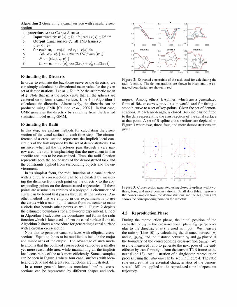
In its simplest form, the radii function of a canal surfacewith a circular cross-section can be calculated by measur-ing the distance from each point on the directrix to the cor-responding points on the demonstrated trajectories. If thesepoints are assumed as vertices of a polygon, a circumscribedcircle can be found that passes through all the vertices. An-other method that we employ in our experiments is to usethe vertex with a maximum distance from the center to makea circle that bounds other points as well. Figure 2 depictsthe estimated boundaries for a real-world experiment. Line 5in Algorithm 1 calculates the boundaries and forms the radiifunction which is later used to form the canal surface (Line 6).Algorithm 2 shows a procedure for generating a canal surfacewith a circular cross-section.

Note that to generate canal surfaces with elliptical cross-sections, Equation 9 has to be modified to include the majorand minor axes of the ellipse. The advantage of such modi-fication is that the obtained cross-section can cover a smalleryet more reasonable area while maintaining all the implicitlocal constraints of the task more efficiently. Some examplescan be seen in Figure 1 where four canal surfaces with iden-tical directrix and different radii functions are illustrated.

In a more general form, as mentioned before, cross-sections can be represented by different shapes and tech-

0 1000 2000

-0.5

0

0.5

1

1.5X

0 1000 2000

0.4

0.6

0.8

1

1.2Y

0 1000 2000

-0.05

0

0.05

0.1Z

0 1000 2000

-0.2

-0.1

0

0.1

0.2

0.3Bound X

0 1000 2000

-0.3

-0.2

-0.1

0

0.1

0.2Bound Y

0 1000 2000

-0.04

-0.02

0

0.02

0.04

0.06Bound Z

Figure 2: Extracted constraints of the task used for calculating theradii function. The demonstrations are shown in black and the ex-tracted boundaries are shown in red.

niques. Among others, B-splines, which are a generalizedform of Bezier curves, provide a powerful tool for fitting asmooth curve to a set of key-points. Given the set of demon-strations, at each arc-length, a closed B-spline can be fittedto the data representing the cross-section of the canal surfaceat that point. A set of B-spline cross-sections are depicted inFigure 3 where two, three, four, and more demonstrations aregiven.

-2 0 2

-2

0

2

-1 -0.5 0 0.5 1

-0.5

0

0.5

1

-1 -0.5 0 0.5 1

-0.5

0

0.5

1

-1 -0.5 0 0.5 1-0.5

0

0.5

1

Figure 3: Cross-section generated using closed B-splines with two,three, four, and more demonstrations. Small dots (blue) representthe points sampled from the demonstrations and the big (blue) dotshows the corresponding point on the directrix.

4.2 Reproduction PhaseDuring the reproduction phase, the initial position of theend-effector p0 in the cross-sectional plane S0 (perpendic-ular to the directrix at c0) is used as input. We measurethe ratio η (Line 10) by calculating the distance between p0and c0 (p0c0) and the distance between c0 and g0 placed atthe boundary of the corresponding cross-section (g0c0). Weuse the measured ratio to generate the next pose of the end-effector by transforming it from the current TNB frame to thenext (Line 13). An illustration of a single-step reproductionprocess using the ratio rule can be seen in Figure 4. The ratiorule ensures that the essential characteristics of the demon-strated skill are applied to the reproduced time-independenttrajectory.

Si Si+1

m(s)

pi

pi+1

eB

i eB

i+1

eN

ieN

i+1

ci

ci+1

gi

T

Figure 4: Reproduction from a random initial pose pi on the ith

cross-section Si. Firstly the ratio of the initial point is calculated asη = pici

gici. Then the point is transferred to the next cross-section,

Si+1 and scaled by gi+1ci+1 such that pi+1 = η.gi+1ci+1.(Tpi),where T is the transformation matrix between two frames.

Dealing with NoiseCalculating Frenet-Serret frames for real data is prone tonoise. The reason is that at some points the derivative vec-tor deT

ds vanishes and the formulae cannot be applied anymore(i.e. eN cannot be calculated). Under such circumstance, apossible solution is to produce the unit normal vector eN asthe cross product of a random vector by the unit tangent vec-tor eT .

5 ExperimentsTo validate the capabilities and interpretability of the pro-posed approach, we performed a set of experiments usingboth artificially made and real demonstrations. The simu-lated experiments show the capabilities of the proposed ap-proach using noiseless data while the real-world experimentshows its feasibility. The real demonstrations were collectedthrough kinesthetic teaching using a 6DOF Jaco2 robotic armfrom Kinova. The data is recorded at a sampling rate of 30Hz.

5.1 Task IConsider four simulated demonstrations as illustrated in Fig-ure 5. The demonstrations imply that the motion can beginand end in a wide task-space but it is constrained in the middleand has to pass through a very narrow area. The obtained di-rectrix and the canal surface with a circular cross-section areestimated using Algorithm 1 and are shown in Figure 5. Al-though the directrix of the four identical trajectories becomesa straight line, the canal surface extracts and preserves theimportant features and constraints of the demonstrated task.Given a new initial pose of the end-effector, the reproducedtrajectory using the ratio rule (explained in Section 4.2) startsand finishes inside the canal surface while satisfying the con-straint of the task in the middle.

5.2 Task IIIn this task, one of the demonstrations from the previous setis removed and the experiment is repeated. The result is de-picted in Figure 6. Although the canal surface calculatedin the previous experiment is still valid for this set as well,a better description of the skill can be represented using acanal surface with an elliptical cross-section. The reproduced

Figure 5: Four demonstrations (solid black), directrix (blue) andthe encoded canal surface (gray) for task I. The projection of thesurface on the X − Y plane shows the boundaries of the obtainedcanal surface. Reproduction of the motion (dotted black) from arandom initial pose (red marker) is depicted.

trajectory generated using the ratio rule (explained in Sec-tion 4.2) is also illustrated in Figure 6. This experiment in-dicates that after removing a demonstration from the set, thecanal surface adapts to the new situation while maintainingthe constraints of the task. And also, the adaptation of themodel and the reproduced trajectory are fairly predictable.Such features make canal surfaces a promising approach forproducing visually understandable models employable evenby non-expert users.

Figure 6: One of the demonstrations is removed from the previ-ous set and the canal surface is re-generated with an elliptical cross-section (task II). The directrix (blue) is inclined towards the demon-stration on top. Reproduction of the motion (dotted black) from arandom initial pose (red marker) is depicted.

5.3 Task IIIIn this experiments, we collected five demonstrations in task-space using the Jaco2 robotic arm through kinesthetic teach-ing. Figure 2 shows the captured demonstrations and the ex-tracted constraints of the task. The obtained canal surface us-ing Algorithm 1 with an elliptical cross-section is illustratedin Figure 7. The reproduced time-independent trajectory is

generated using the ratio rule as explained in Section 4.2.This experiment shows the feasibility of the proposed ap-proach in real-world experiments.

Figure 7: Captured demonstrations (solid black lines) using theJaco2 robotic arm and the corresponding encoded canal surface. Thedirectrix is shown in blue and the reproduction of the motion from arandom initial pose is plotted with dotted black line.

5.4 Comparing with GMM/GMRWe applied GMM/GMR approach as presented in [Calinon etal., 2007] to the set of real demonstrations from Section 5.3.As shown in Figure 8a, a statistical model is trained usingGMM with 4 Gaussian components, and a generalized ver-sion of the dataset with associated constraints is retrievedthrough GMR. We found that 4 Gaussian components effi-ciently encode the skill. As it can be seen in Figure 8b, com-paring the outcome of GMM/GMR with the results from Sec-tion 5.3 reveals that the reproduced trajectory by GMM/GMRis similar to the directrix of the modeled canal surface. Theobtained representation by using our approach is visuallydescriptive and easily understandable even for non-experts.This feature enables end-users to evaluate the given set ofdemonstrations and improve the learned model by providingproper feedback (e.g. verbal, physical). Another advantageis that our approach reproduces time-independent trajecto-ries from any random initial pose inside the canal. However,GMR reproduces time-based trajectories and requires an ad-ditional component to generate trajectories from an arbitraryinitial pose. Several reproduced trajectories by our approachfrom various initial poses are depicted in figure 9.

6 Discussion and Future WorkOne of the advantages of employing geometrical approachessuch as canal surfaces is that the obtained representation isvisually descriptive and easily understandable even for non-expert users. This feature enables end-users to evaluate thegiven set of demonstrations and improve the learned modelby providing proper feedback (e.g. verbal, physical). Un-like many existing LfD approaches in which the human op-erator is only at the beginning of the process, our approachis capable of keeping the user in the loop. For instance, ifby observing the obtained model the end-user realizes thatthe canal needs to be more constrained at some specific area,the model can be updated by removing some of the trajecto-ries and adding new ones. Making such decisions to adjustthe model would be very complicated for non-experts whiledealing with representations such as DMPs and GPs.

500 1000 1500 2000-0.5

0

0.5

1

1.5X

500 1000 1500 20000.4

0.6

0.8

1

1.2Y

500 1000 1500 2000-0.05

0

0.05

0.1Z

500 1000 1500 2000X

-0.5

0

0.5

1

1.5

Y

500 1000 1500 2000X

0.4

0.6

0.8

1

1.2

Z

500 1000 1500 2000Y

-0.05

0

0.05

0.1

Z

(a) Result from GMM/GMR.

0 1000 2000-2

0

2X

CSGMM

0 1000 20000.5

1

1.5Y

CSGMM

0 1000 2000-0.05

0

0.05Z

CSGMM

(b) Directrix vs. GMR reproduction.

Figure 8: Comparing the proposed approach with GMM/GMR.

-0.1

0.2

0Z

0.1

0.4

0.60

Y

0.80.5

X

1

11.2

Figure 9: Demonstrations (black), directrix (blue), GMR repro-duction (orange), and multiple reproductions from arbitrary initialpoints (yellow) using our approach, for task III.

Another merit of our approach is that unlike many existingapproaches the reproduced trajectories are time-independent.This feature enables our approach to reproduce trajectoriesreactively from any point inside the canal surface.

The proposed approach can be adapted to the adjustmentsand constraints applied even during the reproduction phase.Our future work includes activating the robot in compliantcontrol mode to enable the user to interact and refine therobot’s movements during reproduction. The learned modelcan be actively updated based on the physical correctionsfrom the user. The new reproduced trajectories based on theupdated model will reflect the given feedback in the form ofnew constraints on the surface.

Furthermore, although the proposed approach is capableof encoding and reproducing trajectories on its own, it can becombined with other methods such as DMPs and keyframe-based LfD [Akgun et al., 2012]. Integration with DMPscan provide us with a different reproduction method whilekeyframe-based LfD enables the system to take advantage ofsmoother trajectories while retaining their important charac-teristics.

References[Abbena et al., 2006] Elsa Abbena, Simon Salamon, and Al-

fred Gray. Modern differential geometry of curves and sur-faces with Mathematica. CRC press, 2006.

[Ahmadzadeh and Chernova, 2016] Seyed Reza Ah-madzadeh and Sonia Chernova. A geometric approach forencoding demonstrations and learning new trajectories. InRobotics: Science and Systems (RSS 2016), Workshop onPlanning for Human-Robot Interaction: Shared Autonomyand Collaborative Robotics, pages 1–3, Ann Arbor, MI,USA, June 2016. IEEE.

[Akgun et al., 2012] Baris Akgun, Maya Cakmak, KarlJiang, and Andrea L. Thomaz. Keyframe-based learn-ing from demonstration. International Journal of SocialRobotics, 4(4):343–355, 2012.

[Argall et al., 2009] Brenna D. Argall, Sonia Chernova,Manuela Veloso, and Brett Browning. A survey of robotlearning from demonstration. Robotics and autonomoussystems, 57(5):469–483, 2009.

[Calinon et al., 2007] Sylvain Calinon, Florent Guenter, andAude Billard. On learning, representing, and general-izing a task in a humanoid robot. Systems, Man, andCybernetics, Part B: Cybernetics, IEEE Transactions on,37(2):286–298, 2007.

[Dong and Williams, 2012] Shuonan Dong and BrianWilliams. Learning and recognition of hybrid manipula-tion motions in variable environments using probabilisticflow tubes. International Journal of Social Robotics,4(4):357–368, 2012.

[Farouki and Sverrisson, 1996] Rida Amt Farouki and Rag-nar Sverrisson. Approximation of rolling-ball blends forfree-form parametric surfaces. Computer-Aided Design,28(11):871–878, 1996.

[Grimes et al., 2006] David B. Grimes, Rawichote Chalod-horn, and Rajesh PN Rao. Dynamic imitation in a hu-manoid robot through nonparametric probabilistic infer-ence. In Robotics: science and systems, pages 199–206.Cambridge, MA, 2006.

[Hartmann, 2003] E Hartmann. Geometry and algorithmsfor computer aided design. Darmstadt University of Tech-nology, 2003.

[Hilbert and Cohn-Vossen, 1952] David Hilbert and StephanCohn-Vossen. Geometry and the imagination. Chelsea,New York, 1952.

[Ijspeert et al., 2002] Auke J. Ijspeert, Jun Nakanishi, andStefan Schaal. Movement imitation with nonlinear dy-namical systems in humanoid robots. In Robotics and Au-tomation (ICRA), 2002 IEEE International Conference on,volume 2, pages 1398–1403. IEEE, 2002.

[Ijspeert et al., 2013] Auke J. Ijspeert, Jun Nakanishi, HeikoHoffmann, Peter Pastor, and Stefan Schaal. Dynamicalmovement primitives: learning attractor models for motorbehaviors. Neural computation, 25(2):328–373, 2013.

[Majumdar and Tedrake, 2016] Anirudha Majumdar andRuss Tedrake. Funnel libraries for real-time robust feed-back motion planning. arXiv preprint arXiv:1601.04037,2016.

[Reiner et al., 2014] Benjamin Reiner, Wolfgang Ertel,Heiko Posenauer, and Markus Schneider. Lat: A simplelearning from demonstration method. In IntelligentRobots and Systems (IROS), 2014 IEEE/RSJ InternationalConference on, pages 4436–4441. IEEE, 2014.

[Schneider and Ertel, 2010] Markus Schneider and Wolf-gang Ertel. Robot learning by demonstration with localgaussian process regression. In Intelligent Robots and Sys-tems (IROS), 2010 IEEE/RSJ International Conference on,pages 255–260. IEEE, 2010.

[Shani and Ballard, 1984] Uri Shani and Dana H Ballard.Splines as embeddings for generalized cylinders. Com-puter Vision, Graphics, and Image Processing, 27(2):129–156, 1984.

[Shanmugavel et al., 2007] Madhavan Shanmugavel, Anto-nios Tsourdos, Rafał Zbikowski, and Brian A White. 3dpath planning for multiple uavs using pythagorean hodo-graph curves. In AIAA Guidance, Navigation, and Con-trol Conference and Exhibit, Hilton Head, South Carolina,pages 20–23, 2007.

[Vijayakumar et al., 2005] Sethu Vijayakumar, AaronD’souza, and Stefan Schaal. Incremental online learningin high dimensions. Neural computation, 17(12):2602–2634, 2005.