enabling utility-scale electrical energy storage through
TRANSCRIPT

Enabling Utility-Scale Electrical Energy
Storage through Underground
Hydrogen-Natural Gas Co-Storage
by
Dan Peng
A thesis
presented to the University of Waterloo
in fulfillment of the
thesis requirement for the degree of
Master of Applied Science
in
Chemical Engineering
Waterloo, Ontario, Canada, 2013
©Dan Peng 2013

AUTHOR'S DECLARATION
I hereby declare that I am the sole author of this thesis. This is a true copy of the thesis, including any
required final revisions, as accepted by my examiners.
I understand that my thesis may be made electronically available to the public.
ii

Abstract
Energy storage technology is needed for the storage of surplus baseload generation and the storage of
intermittent wind power, because it can increase the flexibility of power grid operations. Underground
storage of hydrogen with natural gas (UHNG) is proposed as a new energy storage technology, to be
considered for utility-scale energy storage applications. UHNG is a composite technology: using
electrolyzers to convert electrical energy to chemical energy in the form of hydrogen. The latter is
then injected along with natural gas into existing gas distribution and storage facilities. The energy
stored as hydrogen is recovered as needed; as hydrogen for industrial and transportation applications,
as electricity to serve power demand, or as hydrogen-enriched natural gas to serve gas demand. The
storage of electrical energy in gaseous form is also termed “Power to Gas”. Such large scale electrical
energy storage is desirable to baseload generators operators, renewable energy-based generator
operators, independent system operators, and natural gas distribution utilities. Due to the low density
of hydrogen, the hydrogen-natural gas mixture thus formed has lower volumetric energy content than
conventional natural gas. But, compared to the combustion of conventional natural gas, to provide the
same amount of energy, the hydrogen-enriched mixture emits less carbon dioxide.
This thesis investigates the dynamic behaviour, financial and environmental performance of UHNG
through scenario-based simulation. A proposed energy hub embodying the UHNG principle, located
in Southwestern Ontario, is modeled in the MATLAB/Simulink environment. Then, the performance
of UHNG for four different scenarios are assessed: injection of hydrogen for long term energy
storage, surplus baseload generation load shifting, wind power integration and supplying large
hydrogen demand. For each scenario, the configuration of the energy hub, its scale of operation and
operating strategy are selected to match the application involved. All four scenarios are compared to
the base case scenario, which simulates the operations of a conventional underground gas storage
facility.
For all scenarios in which hydrogen production and storage is not prioritized, the concentration of
hydrogen in the storage reservoir is shown to remain lower than 7% for the first three years of
operation. The simulation results also suggest that, of the five scenarios, hydrogen injection followed
by recovery of hydrogen-enriched natural gas is the most likely energy recovery pathway in the near
future. For this particular scenario, it was also found that it is not profitable to sell the hydrogen-
iii

enriched natural gas at the same price as regular natural gas. For the range of scenarios evaluated, a
list of benchmark parameters has been established for the UHNG technology. With a roundtrip
efficiency of 39%, rated capacity ranging from 25,000 MWh to 582,000 MWh and rated power from
1 to 100 MW, UHNG is an energy storage technology suitable for large storage capacity, low to
medium power rating storage applications.
iv

Acknowledgements
The research included in this thesis could not have been performed if not for the assistance, patience,
and support of many individuals.
First and foremost, I would like to thank my supervisors, Prof. Ali Elkamel and Prof. Michael Fowler
for mentoring me over the course of this two year journey. Their insights are at the origin of this
project, and they have been great sources of academic and professional inspirations.
My gratitude is also extended to past and present members of my research group: much of my work is
based on the previous ground covered by my colleagues Yaser Maniyali, Faraz Syed and Abduslam
Mohamed Sharif, and I am very thankful of Lisa Tong, Andreas Mertes, Ivan Kantor and Leila
Ahmadi for your good company.
I would like to thank my parents and my friends, whose patient company and encouragement helped
me progress when I most needed it, especially Tianyu for offering to read my manuscript.
Finally, my appreciation is extended to the Natural Sciences and Engineering Research Council of
Canada and to University of Waterloo for their sponsorship throughout this program.
v

Dedication
I dedicate this thesis to my grandfather, Baozhang He, the first chemical engineer in my family. He
had taught me important lessons in perseverance and kindness. May he rest in peace.
vi

Table of Contents
AUTHOR'S DECLARATION ............................................................................................................... ii
Abstract ................................................................................................................................................. iii
Acknowledgements ................................................................................................................................ v
Dedication ............................................................................................................................................. vi
Table of Contents ................................................................................................................................. vii
List of Figures ...................................................................................................................................... xii
List of Tables ..................................................................................................................................... xviii
List of Acronyms ................................................................................................................................. xxi
Chapter 1 Introduction ........................................................................................................................... 1
1.1 Research Motivation ..................................................................................................... 2
1.2 Research Objective and Approach ................................................................................ 7
1.3 Project Scope ................................................................................................................ 9
1.3.1 Physical Model ...................................................................................................... 9
1.3.2 Performance Model ............................................................................................. 10
Chapter 2 Literature Review ............................................................................................................... 12
2.1 Energy Storage ............................................................................................................ 12
2.1.1 Electricity Supply Chain ..................................................................................... 14
2.1.2 Applications of Storage in the Existing Grid ...................................................... 18
2.1.3 Applications of Storage in the Future Grid ......................................................... 23
2.1.4 Conventional Energy Storage Technologies ....................................................... 26
2.2 The Case for Ontario ................................................................................................... 38
2.3 Energy Hub Framework .............................................................................................. 41
2.3.1 Definition ............................................................................................................ 41
2.3.2 Methodology ....................................................................................................... 42
2.3.3 Applications ........................................................................................................ 45
2.4 Key Technologies ....................................................................................................... 46
2.4.1 Electrolysis .......................................................................................................... 48
2.4.2 Underground Gas Storage ................................................................................... 52
2.4.3 Gas Turbines ....................................................................................................... 59
2.4.4 Hydrogen Recovery and Use .............................................................................. 65
vii

2.4.5 Distribution of Hydrogen Enriched Natural Gas ................................................ 69
Chapter 3 Model Overview ................................................................................................................. 73
3.1 Energy Hub Overview ................................................................................................ 73
3.2 Decision Variables ...................................................................................................... 75
3.3 Exogenous Variables .................................................................................................. 78
3.3.1 Power Grid .......................................................................................................... 80
3.3.2 Natural Gas Grid ................................................................................................. 86
3.3.3 Mixture Demand ................................................................................................. 89
3.3.4 Hydrogen Demand .............................................................................................. 91
3.4 Performance indicators ............................................................................................... 95
Chapter 4 Physical Model Development ........................................................................................... 101
4.1 Storage Reservoir ...................................................................................................... 104
4.1.1 Storage Capacity and Inventory ........................................................................ 104
4.1.2 Injectability and Deliverability ......................................................................... 115
4.1.3 Rate of Change for Injectability and Deliverability .......................................... 122
4.2 Wind Turbines .......................................................................................................... 126
4.2.1 Efficiency .......................................................................................................... 126
4.2.2 Rated power ...................................................................................................... 128
4.2.3 Ramp rate .......................................................................................................... 128
4.3 Electrolyzer ............................................................................................................... 130
4.3.1 Efficiency .......................................................................................................... 130
4.3.2 Rated Power ...................................................................................................... 132
4.3.3 Ramp Rate ......................................................................................................... 134
4.4 Gas Turbine ............................................................................................................... 137
4.4.1 Efficiency .......................................................................................................... 137
4.4.2 Rated power ...................................................................................................... 147
4.4.3 Ramp rate .......................................................................................................... 148
4.5 Separator ................................................................................................................... 151
4.5.1 Efficiency .......................................................................................................... 151
4.5.2 Rated power ...................................................................................................... 153
4.5.3 Ramp rate .......................................................................................................... 154
4.6 Compressor ............................................................................................................... 156
viii

4.6.1 Compression Efficiency .................................................................................... 156
4.6.2 Rated Power ...................................................................................................... 158
4.6.3 Ramp Rate ......................................................................................................... 158
Chapter 5 Financial Model Development ........................................................................................... 161
5.1 Annual Sales of Energy Products ............................................................................. 161
5.2 Annual Purchases of Energy Inputs .......................................................................... 165
5.3 Inventoriable Cost of Purchase ................................................................................. 167
5.4 Capital Cost ............................................................................................................... 170
5.4.1 Wind Turbines .................................................................................................. 170
5.4.2 Electrolyzers ..................................................................................................... 170
5.4.3 Separator ........................................................................................................... 171
5.4.4 CCGT ................................................................................................................ 173
5.4.5 Compressors ...................................................................................................... 173
5.5 Operating and Maintenance Cost .............................................................................. 177
Chapter 6 Emission Model Development .......................................................................................... 179
6.1 Net Emissions ........................................................................................................... 179
6.2 Emissions Incurred ................................................................................................... 179
6.2.1 Gas Compression .............................................................................................. 180
6.2.2 Electrolyzer Power Supply................................................................................ 180
6.2.3 On-Site CCGT Generation ................................................................................ 181
6.2.4 HENG Mixture Consumption ........................................................................... 181
6.3 Emissions Mitigated ................................................................................................. 181
6.3.1 Hydrogen from Steam Methane Reforming ...................................................... 181
6.3.2 Gas-Fired CCGT Generation ............................................................................ 182
6.3.3 Natural Gas Consumption ................................................................................. 182
Chapter 7 Scenario Generation .......................................................................................................... 184
7.1 Base Case Scenario: Underground Gas Storage ....................................................... 184
7.1.1 Summary ........................................................................................................... 184
7.1.2 Decision Point Model Logic ............................................................................. 186
7.2 Mid-Term Scenario: Hydrogen Injection .................................................................. 190
7.2.1 Summary ........................................................................................................... 190
7.2.2 Decision Point Modeling Logic ........................................................................ 191
ix
7.3 Long-Term Scenario: Reduction of Surplus Baseload (SGB) Generation ............... 196
7.3.1 Summary ........................................................................................................... 196
7.3.2 Decision Point Modeling Logic ........................................................................ 198
7.4 Long-Term Scenario: Integration of Wind Power .................................................... 201
7.4.1 Summary ........................................................................................................... 202
7.4.2 Decision Point Modeling Logic ........................................................................ 203
7.5 Long-Term Scenario: Meeting Large Hydrogen Demand ........................................ 207
7.5.1 Summary ........................................................................................................... 207
7.5.2 Decision Point Modeling Logic ........................................................................ 209
Chapter 8 Simulation Results ............................................................................................................. 214
8.1 Base Case Scenario: Underground Gas Storage ....................................................... 214
8.2 Mid-Term Scenario: Hydrogen Injection .................................................................. 222
8.3 Long-Term Scenario: Surplus Baseload Generation (SBG) Reduction .................... 231
8.4 Long-Term Scenario: Integration of Wind Power .................................................... 242
8.5 Long-Term Scenario: Meeting Large Hydrogen Demand ........................................ 253
8.6 Energy Storage Benchmark Parameters .................................................................... 264
8.6.1 Roundtrip Efficiency ......................................................................................... 264
8.6.2 Rated Capacity .................................................................................................. 264
8.6.3 Rated Power ...................................................................................................... 266
8.6.4 Self-Discharge rate ............................................................................................ 268
8.6.5 Durability .......................................................................................................... 269
8.6.6 Cost of Storage .................................................................................................. 269
Chapter 9 Results Discussion ............................................................................................................. 271
9.1 Base Case Scenario Validation ................................................................................. 271
9.2 Effect of Decision Variables on Financial Performance Indicators .......................... 274
9.2.1 Financial Performance Baseline ........................................................................ 274
9.2.2 On Hydrogen Injection...................................................................................... 278
9.2.3 On SBG Reduction ........................................................................................... 279
9.2.4 On Wind Power Integration .............................................................................. 280
9.2.5 On Large Hydrogen Demand ............................................................................ 281
9.3 Effect of Decision Variables on Environmental Performance Indicators ................. 284
Chapter 10 Conclusion ....................................................................................................................... 287
x

10.1 Key Decision Variables .......................................................................................... 287
10.2 Physical Constraints ................................................................................................ 288
10.3 Benchmark Parameters ........................................................................................... 290
10.4 Performance Indicators ........................................................................................... 290
10.5 Simulation Scenarios .............................................................................................. 291
10.6 Assessment of Scenarios ......................................................................................... 292
10.7 Recommendations for Future Research .................................................................. 294
References .......................................................................................................................................... 298
xi

List of Figures
Figure 1.1Traditional paradigm for power grid management ................................................................ 2
Figure 1.2 Proposed new paradigm for power grid management with energy storage facilities............ 4
Figure 1.3 Milestones of simulation project ........................................................................................... 8
Figure 1.4 Project scope for the physical model .................................................................................... 9
Figure 1.5 Structure of the performance model .................................................................................... 10
Figure 1.6 Comparison of economic and financial analysis ................................................................. 11
Figure 2.1 Global energy flow for societies [13] .................................................................................. 13
Figure 2.2 Stages in the electricity supply chain .................................................................................. 14
Figure 2.3 Ontario power generation by type for June 30th, 2013 [14] ............................................... 17
Figure 2.4 Conceptual diagram for baseload power generation shifting .............................................. 19
Figure 2.5 Scope of analysis for generation shifting ............................................................................ 20
Figure 2.6 Scope of analysis for grid congestion relief ........................................................................ 21
Figure 2.7 Scope of analysis for end-use energy reliability and cost reduction ................................... 23
Figure 2.8 Hypothetical weekly grid supply scenario with high wind power penetration ................... 25
Figure 2.10 Operational benefits monetizing the value of energy storage [10] ................................... 26
Figure 2.11 Energy storage technologies by power ratings and discharge time [10] .......................... 36
Figure 2.12 Ontario’s installed generation capacity by type [22] ........................................................ 38
Figure 2.13 Total electricity output by fuel type [2] ............................................................................ 39
Figure 2.14 Number of hour per month with negative HOEP [14] ...................................................... 40
Figure 2.15 Generic schematic of an energy hub [24] ......................................................................... 42
Figure 2.16 Storage elements in energy hubs [25] ............................................................................... 44
Figure 2.17 Process diagram of alkaline electrolysis [44] .................................................................... 49
Figure 2.18 Energy demand for water and steam electrolysis [41] ...................................................... 51
Figure 2.19 Type of reservoirs for worldwide UGS [48] ..................................................................... 53
Figure 2.20 Confined and unconfined aquifers (National Ground Water Association, 2007) ............. 55
Figure 2.21 Installed maximum working volumes of Ontario UGS facilities ...................................... 58
Figure 2.22 Block diagram of a gas turbine for power generation [56] ............................................... 59
Figure 2.23 Block diagram for combined cycle gas turbine ................................................................. 61
Figure 2.24 Effect of hydrogen-natural gas mixtures on the Wobbe Index [59] .................................. 63
xii

Figure 2.25 Effect of hydrogen concentration in a CH4-H2 mixture on carbon emissions, relative to
pure CH4 [60] ....................................................................................................................................... 64
Figure 2.26 Two-column four-step Skarstorm cycle [64] .................................................................... 69
Figure 2.27 Energy-transport losses for hydrogen and hydrogen-natural gas mixtures, assuming an
unchanged pressure drop [59] .............................................................................................................. 71
Figure 3.1 Detailed view of the energy hub ......................................................................................... 74
Figure 3.2 Interaction between the power grid and energy hub ........................................................... 80
Figure 3.3 Ontario's power grid and its transmission zones [73] ......................................................... 81
Figure 3.4 Historic HOEP from 2010-2012 ......................................................................................... 82
Figure 3.5 Historic Ontario electricity demand for 2010-2012 ............................................................ 83
Figure 3.6 Correlation between 2010-2012 electricity demand and HOEP for Ontario ...................... 83
Figure 3.7 Relative hourly changes in HOEP and Ontario demand ..................................................... 84
Figure 3.8 Hourly emission factors for power generation in Ontario for 2010-2012 ........................... 85
Figure 3.9 Interaction of the natural gas grid with the energy hub ....................................................... 86
Figure 3.10 Pipeline Infrastructure in Ontario [76] .............................................................................. 87
Figure 3.11 Historic natural gas spot price at Henry Hub for 2010-2012 ............................................ 88
Figure 3.12 Interaction of the mixture need with energy hub .............................................................. 89
Figure 3.13 Ontario monthly natural gas demand for 2010 – 2012 [77] .............................................. 90
Figure 3.14 Interaction of Hydrogen Need with Energy Hub .............................................................. 91
Figure 3.15 Historic retail price of regular gasoline from 1991 to 2012 .............................................. 93
Figure 3.16 Linear dependences of natural gas and coal prices to centralized and distributed SMR and
coal based hydrogen costs [81] ............................................................................................................. 94
Figure 3.17 Scope for financial model ................................................................................................. 98
Figure 3.18 Scope for emission model ................................................................................................. 99
Figure 4.1 Mass balance difference between converters and storage devices .................................... 102
Figure 4.2 Architecture of the energy hub physical model ................................................................ 103
Figure 4.3 Reservoir maximum inventory and mixture compressibility factor for stored gas mixture of
different hydrogen concentrations ...................................................................................................... 112
Figure 4.4 Reservoir cushion gas requirement and mixture compressibility factor for stored gas
mixture of different hydrogen concentrations .................................................................................... 114
Figure 4.5 Maximum working gas volume available and cushion gas requirement for different
hydrogen concentration in stored mixture .......................................................................................... 114
xiii

Figure 4.6 Shut-in wellhead pressure as a function of reservoir pressure .......................................... 116
Figure 4.7 Reservoir flow rate as function of reservoir and wellhead pressure ................................. 121
Figure 4.8 Wellhead pressure as a function of reservoir dispatch order ............................................ 123
Figure 4.9 Model flow diagram for electrolyzers ............................................................................... 124
Figure 4.10 Power curve for V90 2.0MW wind turbine [69] ............................................................. 126
Figure 4.11 Hourly wind speed at Sarnia for 2010-2012 [87] ............................................................ 127
Figure 4.12 Model flow diagram for wind turbines ........................................................................... 129
Figure 4.13 Electrolyzer stack efficiency as a function of current density ........................................ 131
Figure 4.14 Correlation between the hydrogen output based utilization factor and the power
consumption based utilization factor for the electrolyzer .................................................................. 134
Figure 4.15 Model flow diagram for electrolyzers ............................................................................. 136
Figure 4.16 Process flow diagram for the combined-cycle plant ....................................................... 137
Figure 4.17 Temperature profile along the HRSG ............................................................................. 143
Figure 4.18 Gas turbine cycle efficiency as a function of fuel hydrogen concentration and relative fuel
rate ...................................................................................................................................................... 145
Figure 4.19 Relative efficiencies of the gas turbine cycle and of the combine cycle at part-load
conditions [58] .................................................................................................................................... 146
Figure 4.20 Relative combined cycle efficiency as a function of relative gas turbine cycle efficiency
............................................................................................................................................................ 147
Figure 4.21 Model flow diagram for CCGT ...................................................................................... 150
Figure 4.22 Model flow diagram for the separator ............................................................................. 155
Figure 4.23 Heat capacity ratio as a function of hydrogen concentration in compression mixture ... 158
Figure 4.24 Model flow diagram for the compressor ......................................................................... 160
Figure 5.1 Points of sales of energy products from the energy hub ................................................... 163
Figure 5.2 Points of purchases of energy products for the energy hub .............................................. 165
Figure 5.3 Capital cost factor of compressors for different installed capacity[104] .......................... 174
Figure 7.1 Model scope for the base case scenario ............................................................................ 185
Figure 7.2 Reservoir operation decision point (D1) for the base case scenario ................................. 186
Figure 7.3 Natural gas market price and its 26 weeks moving average for years 2010-2012 ............ 187
Figure 7.4 Gas blending decision point (D4) for base case scenario .................................................. 188
Figure 7.5 Mixture dispatch decision block (D5) for the base case scenario ..................................... 189
Figure 7.6 Model scope for hydrogen injection scenario ................................................................... 191
xiv
Figure 7.7 Electrolyzer power supply decision point (D2) for the hydrogen injection scenario ........ 193
Figure 7.8 Ontario power price and its 24 hours moving average for years 2010-2012 .................... 193
Figure 7.9 Hydrogen bypass decision point (D3) for the hydrogen injection scenario ...................... 194
Figure 7.10 Gas blending decision point (D4) for hydrogen injection scenario................................. 195
Figure 7.11 Model scope for the SBG reduction scenario ................................................................. 197
Figure 7.12 Reservoir operation decision point (D1) for the SBG reduction scenario ...................... 198
Figure 7.13 Electricity demand in Ontario and its one-year moving average for 2010-2012 ............ 199
Figure 7.14 Electrolyzer power supply decision block (D2) for the SBG reduction scenario ........... 200
Figure 7.15 Mixture dispatch decision block (D5) for the SBG reduction scenario .......................... 201
Figure 7.16 Model scope for the wind power integration scenario .................................................... 202
Figure 7.17 Reservoir operation decision point (D1) for the wind power integration scenario ......... 204
Figure 7.18 Electrolyzer power supply decision point (D2) for the wind power integration scenario
............................................................................................................................................................ 205
Figure 7.19 Model scope for the large hydrogen demand scenario .................................................... 207
Figure 7.20 Reservoir operation decision point (D1) for the large hydrogen demand scenario ......... 209
Figure 7.21 Hydrogen bypass decision point (D3) for the large hydrogen demand scenario ............ 210
Figure 7.22 Gas blending decision point (D4) for large hydrogen demand scenario ......................... 211
Figure 7.23 Mixture dispatch decision block (D5) for the large hydrogen demand scenario ............ 212
Figure 7.24 Separator recycle decision point (D6) for the large hydrogen demand scenario ............ 213
Figure 8.1 Dispatch to reservoir for the base case scenario ............................................................... 215
Figure 8.2 Injectability/deliverability and actual reservoir flow rates for the base case scenario ...... 215
Figure 8.3 Reservoir conditions for the base case scenario ................................................................ 216
Figure 8.4 Flow rates of injected streams for the base case scenario ................................................. 217
Figure 8.5 Dispatch of the produced mixture for the base case scenario ........................................... 217
Figure 8.6 Value of inventory for the base case scenario ................................................................... 218
Figure 8.7 Dispatch to reservoir for the hydrogen injection scenario ................................................ 222
Figure 8.8 Injectability/deliverability and actual reservoir flow rates for the hydrogen injection
scenario ............................................................................................................................................... 223
Figure 8.9 Reservoir conditions for the hydrogen injection scenario ................................................. 224
Figure 8.10 Power supply to the electrolyzers in the hydrogen injection scenario ............................ 224
Figure 8.11 Electrolyzer utilization for the hydrogen injection scenario ........................................... 225
Figure 8.12 Outcome of electrolytic hydrogen produced for the hydrogen injection scenario .......... 225
xv

Figure 8.13 Flow rates of injected streams for the hydrogen injection scenario ................................ 226
Figure 8.14 Dispatch of the produced mixture for the hydrogen injection scenario .......................... 227
Figure 8.15 Value of inventory for the hydrogen injection scenario .................................................. 227
Figure 8.16 Dispatch to reservoir for the SBG reduction scenario ..................................................... 231
Figure 8.17 Daily average of dispatch to reservoir for the SBG reduction scenario .......................... 232
Figure 8.18 Injectability/deliverability and actual reservoir flow rates for the SBG reduction scenario
............................................................................................................................................................ 232
Figure 8.19 Reservoir conditions for the SBG reduction scenario ..................................................... 233
Figure 8.20 Power supply to the electrolyzers in the SBG reduction scenario .................................. 234
Figure 8.21 Electrolyzer utilization for the SBG reduction scenario ................................................. 234
Figure 8.22 Outcome of electrolytic hydrogen produced for the SBG reduction scenario ................ 235
Figure 8.23 Flow rates of injected streams for the SBG reduction scenario ...................................... 236
Figure 8.24 Dispatch of the produced mixture for the SBG reduction scenario ................................ 237
Figure 8.25 CCGT utilization for the SBG reduction scenario .......................................................... 238
Figure 8.26 Value of inventory for the SBG reduction scenario ........................................................ 238
Figure 8.27 Daily average of dispatch to reservoir for the wind power integration scenario ............ 242
Figure 8.28 Injectability/deliverability and actual reservoir flow rates for the wind power integration
scenario ............................................................................................................................................... 243
Figure 8.29 Reservoir conditions for the wind power integration scenario ....................................... 244
Figure 8.30 Wellhead pressure and reservoir pressure during March 2010 for the wind power
integration scenario ............................................................................................................................ 245
Figure 8.31 Wind turbines utilization for the wind power integration scenario ................................. 246
Figure 8.32 Power supply to the electrolyzers in the wind power integration scenario ..................... 246
Figure 8.33 Electrolyzer utilization for the wind power integration scenario .................................... 247
Figure 8.34 Outcome of electrolytic hydrogen produced for the wind power integration scenario ... 247
Figure 8.35 Flow rates of injected streams for the wind integration scenario .................................... 248
Figure 8.36 CCGT utilization for the wind power integration scenario ............................................. 248
Figure 8.37 Value of inventory for the wind power integration scenario .......................................... 249
Figure 8.38 Daily average of dispatch to reservoir for the large hydrogen demand scenario ............ 253
Figure 8.39 Injectability/deliverability and actual reservoir flow rates for the large hydrogen demand
scenario ............................................................................................................................................... 254
Figure 8.40 Reservoir conditions for the large hydrogen demand scenario ....................................... 255
xvi

Figure 8.41 Power supply to the electrolyzers in the large hydrogen demand scenario ..................... 255
Figure 8.42 Electrolyzer utilization for the large hydrogen demand scenario.................................... 256
Figure 8.43 Power supply to the electrolyzers in the large hydrogen demand scenario ..................... 256
Figure 8.44 Dispatch of the produced mixture for the large hydrogen demand scenario ................... 257
Figure 8.45 Separator utilization for the large hydrogen demand scenario ........................................ 258
Figure 8.46 Hydrogen delivered to customers for the large hydrogen demand scenario ................... 258
Figure 8.47 Hydrogen concentration of mixture delivered for the large hydrogen demand scenario 259
Figure 8.48 Value of inventory for the large hydrogen demand scenario .......................................... 260
Figure 8.49 The Power to Power pathway for the energy hub ........................................................... 264
Figure 8.50 Rated storage capacity of UHNG as a function of the reservoir hydrogen concentration
............................................................................................................................................................ 265
Figure 8.51 Rated power of reservoir for UHNG as a function of the stored/discharged mixture
hydrogen concentration ...................................................................................................................... 266
Figure 9.1 Comparison of simulated and actual 2010-2012 inventory level for UGS facilities ........ 271
Figure 9.2 Correlation of simulated and historical gas storage inventory with respect to A) natural gas
price and B) variation in natural gas demand ..................................................................................... 273
Figure 9.3 Waterfall chart for the expected annual cash flow of the base case scenario ................... 274
Figure 9.4 Seasonal and annual trend in natural gas price and demand for 2010-2012 ..................... 275
Figure 9.5 Comparison of financial performance of all scenarios, all values are displayed relative to
the base case value ............................................................................................................................. 276
Figure 9.6 Comparison of operating profits for all scenarios, all values are displayed relative to the
base case value ................................................................................................................................... 277
Figure 9.7 Shares of purchase by components for all scenarios ......................................................... 278
Figure 9.8 Shares of sales by components for all scenarios ............................................................... 278
Figure 9.9 Forecast surplus baseload generation report for July 2013 from the IESO....................... 280
Figure 9.10 Waterfall chart for the expected annual emission of the base case scenario ................... 284
Figure 9.11 Comparison of environmental performance of all scenarios, all values are displayed
relative to the base case value ............................................................................................................ 285
Figure 10.1 Expanded scope for future models assessing the benefits of energy storage via the energy
hub ...................................................................................................................................................... 297
xvii

List of Tables
Table 2.1 Typical life cycle of electricity and its participants .............................................................. 15
Table 2.2 Summary of existing energy storage technology benchmark parameters [6]-[20]. .............. 37
Table 2.3 Summary of utility-scale energy storage technologies ......................................................... 47
Table 2.4 Total and Average working volume of Ontario UGS facilities by type ............................... 58
Table 2.5 Combustion characteristics for hydrogen and methane ........................................................ 62
Table 2.6 Separation methods and their corresponding properties [62] ............................................... 65
Table 2.7 Boiling points of gas mixture components ........................................................................... 67
Table 3.1 List of system configuration and capacity variables ............................................................ 75
Table 3.2 List of decision point inputs and outputs .............................................................................. 77
Table 3.3 List of exogenous environmental variables .......................................................................... 79
Table 3.4 List of physical performance indicators ............................................................................... 96
Table 3.5 List of energy storage benchmark parameters .................................................................... 100
Table 4.1 Differences in constraints for converters and storage devices ........................................... 102
Table 4.2 Molar Composition of Natural Gas [84] ............................................................................ 106
Table 4.3 Compressibility factor of hydrogen/natural gas mixture as a function of pressure,
composition and temperature ............................................................................................................. 107
Table 4.4 Viscosity of hydrogen/natural gas mixture as a function of pressure, composition and
temperature ......................................................................................................................................... 108
Table 4.5 List of key variables and parameters for the reservoir model ............................................ 125
Table 4.6 List of key variables and parameters for wind turbines model ........................................... 128
Table 4.7 List of key variables and parameters for the electrolyzer model ........................................ 135
Table 4.8 List of key variables and parameters for the CCGT model ................................................ 148
Table 4.9 Summary of hydrogen purification PSA processes [92] ................................................... 152
Table 4.10 PSA Process parameters for various feed concentration [93, 94] .................................... 153
Table 4.11 Range of rated hydrogen output for PSA unit .................................................................. 154
Table 4.12 List of key variables and parameters for the separator model .......................................... 154
Table 4.13 Isentropic efficiencies of reciprocating compressors ....................................................... 157
Table 4.14 List of key variables and parameters for the compressor model ...................................... 159
Table 5.1 List of key variables and parameters for the annual sales model ....................................... 164
Table 5.2 List of key variables and parameters for the annual purchase model ................................. 166
xviii

Table 5.3 List of key variables and parameters for the inventoriable purchase cost model ............... 169
Table 5.4 List of key variables and parameters for the capital cost model ........................................ 175
Table 5.5 List of key variables and parameters for the O&M cost model .......................................... 178
Table 6.1 List of key variables and parameters for the emission model ............................................ 182
Table 7.1 Configuration and capacity of energy hub components for the base case scenario ........... 184
Table 7.2 Summary of decision point logic for the base case scenario .............................................. 185
Table 7.3 Configuration and capacity of energy hub components for the hydrogen injection scenario
............................................................................................................................................................ 190
Table 7.4 Summary of decision point logic for the hydrogen injection scenario ............................... 191
Table 7.5 Configuration and capacity of energy hub components for the SBG reduction scenario... 196
Table 7.6 Summary of decision point logic for the SBG reduction scenario ..................................... 197
Table 7.7 Configuration and capacity of energy hub components for the wind power integration
scenario ............................................................................................................................................... 203
Table 7.8 Summary of decision point logic for the wind power integration scenario ........................ 203
Table 7.9 Configuration and capacity of energy hub components for the large hydrogen demand
scenario ............................................................................................................................................... 208
Table 7.10 Summary of decision point logic for the large hydrogen demand scenario ..................... 208
Table 8.1 Summary of physical performance for the base case scenario ........................................... 219
Table 8.2 Summary of financial performance for the base case scenario .......................................... 220
Table 8.3 Net annual cash flow for the base case scenario ................................................................ 221
Table 8.4 Summary of environmental performance for the base case scenario ................................. 221
Table 8.5 Summary of physical performance for the hydrogen injection scenario ............................ 228
Table 8.6 Summary of financial performance for the hydrogen injection scenario ........................... 229
Table 8.7 Net annual cash flow for the hydrogen injection scenario ................................................. 230
Table 8.8 Summary of environmental performance for the hydrogen injection scenario .................. 230
Table 8.9 Summary of physical performance for the SBG reduction scenario .................................. 239
Table 8.10 Summary of financial performance for the SBG reduction scenario ............................... 240
Table 8.11 Net annual cash flow for the SBG reduction scenario ...................................................... 241
Table 8.12 Summary of environmental performance for the SBG reduction scenario ...................... 241
Table 8.13 Summary of physical performance for the wind power integration scenario ................... 250
Table 8.14 Summary of financial performance for the wind power integration scenario .................. 251
Table 8.15 Net annual cash flow for the wind power integration scenario ........................................ 252
xix

Table 8.16 Summary of environmental performance for the wind integration scenario .................... 252
Table 8.17 Summary of physical performance for the large hydrogen demand scenario .................. 261
Table 8.18 Summary of financial performance for the large hydrogen demand scenario .................. 262
Table 8.19 Net annual cash flow for the large hydrogen demand scenario ........................................ 263
Table 8.20 Summary of environmental performance for the large hydrogen demand scenario ......... 263
Table 8.21Rated power of energy hub components for all scenarios ................................................. 267
Table 8.22 Summary of sources of losses for underground hydrogen storage [108] ......................... 268
Table 8.23 Expected lifetime of UHNG technology components [43, 109] ...................................... 269
Table 8.24 Estimated cost of storage for UHNG based on simulation scenarios ............................... 270
Table 9.1 Comparison of average profit per energy unit recovered for different storage pathways .. 283
Table 10.1 Summary of physical constraints used for component models ........................................ 289
Table 10.2 List of energy storage benchmark parameters for UHNG concept .................................. 290
xx

List of Acronyms
CAES Compressed Air Energy Storage
CCGT Combined Cycle Gas Turbine
EIA Energy Information Agency
FIT Feed-In Tariff
HENG Hydrogen-Enriched Natural Gas
IESO Independent Electricity System Operator
NPV Net Present Value
PtoG Power to Gas
PSA Pressure Swing Adsorption
RE Renewable Energy
SBG Surplus Baseload Generation
SMR Steam-Methane Reforming
UGS Underground Gas Storage
UHNG Underground Hydrogen storage with Natural Gas
xxi

Chapter 1 Introduction
Since its foundation in the late 19th century, the electricity grid has operated along one key directive:
the constant matching of power supply and demand across the grid [1]. More than one hundred years
later, the management of today's power grid, a critical infrastructure for modern society, is
encountering new challenges which have led to the study of energy storage technologies.
Underground storage of hydrogen with natural gas (UHNG) is a novel compound technology which is
proposed to provide utility-scale energy storage capacity. This technology revolves around the use of
electrolyzers to convert electrical energy to chemical energy in the form of hydrogen. Hydrogen is
then injected in to natural gas distribution system and natural gas underground storage facilities, along
with the natural gas. This has technological and economic advantages since this technology makes
use of existing natural facilities. Finally, depending on the particular application, the energy stored as
hydrogen can be recovered in different forms: as hydrogen for industrial and transportation
applications, as electricity to serve power demand, or as hydrogen-enriched natural gas to serve gas
demand. UHNG is of special interest for Southwestern Ontario, where there exists extensive
infrastructure for natural gas storage and distribution. The generation of hydrogen from surplus
power and injection of this hydrogen into the natural gas system is generally termed as ‘Power to
Gas’ (PtoG).
Building on the published concept of “energy hub”, a framework which allows for the study of
integrated energy systems, a modeling and simulation study is proposed to better characterize the
UHNG technology. The objective of this thesis is to contribute to a better understanding of the
technology of underground storage of hydrogen with natural gas. This will be accomplished by
investigating its dynamic behaviour, financial and environmental performance through scenario-based
simulation. Results from this research project may be used to inform further research and investment
decisions by technology developers and relevant policy makers.
In the following introduction, the motivation and objective of this study of UHNG is described, and
the scope of the project is defined. In Chapter 2, literature on the topics of energy storage, energy hub,
1

and key component technologies involved in underground storage of hydrogen with natural gas
(UHNG) is reviewed. Chapter 3 specifies the main input, output and exogenous variables used for
modeling. Model development, which relates the detailed structure of the models constructed for this
project, is presented in Chapter 4 through Chapter 6. In Chapter 7, possible sets of input variables are
combined to form scenarios, which yield the results presented in Chapter 8 after simulation. Finally,
the implications of the results are discussed in Chapter 9; key findings and recommendations are
summarized in Chapter 10.
1.1 Research Motivation
Traditionally, power is generated in centralized locations, and then transmitted through great
distances to reach the end users who use electric power to perform various services – mechanical
work, lighting, refrigeration or heating. In order to manage the flow of energy on the grid, grid
operators dispatched orders to the generators, informing them of the action required to balance supply
with demand. Increasingly, grid operators have also engaged in demand management programs, in
which power end-users agree to modify their energy consumption pattern as needed.
Figure 1.1Traditional paradigm for power grid management
Since the 1970s, many nuclear power plants came online and grew to become the dominant baseload
power supplier in several jurisdictions, of which Ontario is an example. In 2011, nuclear power plants
supplied 57% of all electricity generated in the province [2]. Compared to conventional thermal
2

generators, nuclear generators have limited capability to adjust their power output and require long
lead times to change power output; therefore stable operating conditions are preferred. Sometimes,
Ontario’s electricity production from baseload facilities – mostly nuclear, but also including run-of-
the-river hydro and wind – is greater than the provincial demand unless managed. Consequently,
during such periods, electricity produced in Ontario is sometimes exported at a negative price to
neighbouring jurisdictions, or, the baseload facilities are curtailed. It is possible to reduce the power
output from nuclear power plants by manipulating their condenser steam discharge valves, but it is
not the purpose for which such valves have been designed. Such maneuvers increase the risk of
equipment failure, the costs associated with inspections and repairs, while impacting the temperature
of water discharged by the power plant [3]. The Independent Electricity System Operator (IESO) of
Ontario currently forecasts surplus baseload generation (SBG) for a 10 day period to facilitate
coordination between market participants. In its 18-month outlook for the period 2013-2014, the
IESO forecasts a median weekly SBG of 116 to 4608 MW [4].
Concurrently, collective efforts to decrease global carbon emissions and to embrace sustainable
energy resulted in the growth of renewable energy (RE) generators such as wind and solar among the
supply mix. In Ontario, the Feed-in-Tariff (FIT) program has contracted 4,600 MW of non-hydro
renewable energy projects since its inception in 2009. It is on track to increase RE generation to
10,700 MW by 2015 [5]. The inherent intermittency of renewable energy, specifically for wind and
solar, is another cause of concern for grid operators, because renewable energy generators cannot be
dispatched as conventional thermal generators. It is impossible to increase production when the
weather conditions are unfavourable. And, although curtailment is possible during periods of surplus,
the fixed FIT contracts with RE generators make it economically unfavourable to do so. Such loss in
supply flexibility will be felt more acutely as renewable energy generators gain higher penetration in
the grid.
Utility-scale energy storage is seen as a promising solution to address the emerging problems –
surplus baseload generation and increasing intermittency from the deployment of RE generators –
faced by the electric power supply chain, because, energy storage technologies can facilitate grid
operations by providing energy buffering capacity, a new method to regulate the flow of energy
through the power grid.
3
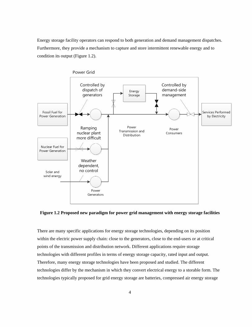
Energy storage facility operators can respond to both generation and demand management dispatches.
Furthermore, they provide a mechanism to capture and store intermittent renewable energy and to
condition its output (Figure 1.2).
Figure 1.2 Proposed new paradigm for power grid management with energy storage facilities
There are many specific applications for energy storage technologies, depending on its position
within the electric power supply chain: close to the generators, close to the end-users or at critical
points of the transmission and distribution network. Different applications require storage
technologies with different profiles in terms of energy storage capacity, rated input and output.
Therefore, many energy storage technologies have been proposed and studied. The different
technologies differ by the mechanism in which they convert electrical energy to a storable form. The
technologies typically proposed for grid energy storage are batteries, compressed air energy storage
4

(CAES), pumped hydro energy storage, advanced capacitors, flywheel energy storage,
superconducting magnetic energy storage, and energy storage through hydrogen [6-11].
Energy storage through the underground storage of hydrogen with natural gas (UHNG) is one of the
new technologies proposed. To store energy using UHNG, electrical energy from the power grid or
other sources is converted to hydrogen via electrolysis. Then, the hydrogen gas is blended with
incoming natural gas to be stored underground; it can also be sent send directly to end users through
the gas distribution system, thus making use of existing natural gas storage and distribution facilities.
If stored, to recover the energy stored, the gas mixture stored underground is retrieved and routed to
one of the three pathways below:
1) Power to Gas: the hydrogen-enriched natural gas is delivered as-is to end-users through the
existing distribution network, performing duties originally performed by natural gas;
2) Power to Power: the gas mixture is sent directly to a combined cycle gas turbine hosted on-site to
generate electricity, which is delivered to the electrical grid or to local demand;
3) Power to Hydrogen: after distribution in the natural gas system or stored with natural gas, the gas
mixture is separated into its components, hydrogen and natural gas, then used-up by distributed
end-users and delivered to end-user via existing pipelines, respectively. Direct production of
hydrogen followed by immediate use, bypassing underground storage, is also a possibility.
Compared to older technologies, pumped hydro storage or battery storage, for example, UHNG is
significantly different, in that:
1) UHNG is a conceptually new composite technology, consisting of technically mature
components;
2) As a composite technology, the performance of UHNG is dependent upon its constituent
technologies, which makes it a more complex physical system than traditional energy storage
technologies;
3) Unlike the more common energy storage technologies, which store and release energy in
reversible pathways, there exist multiple energy recovery pathways for UNHG, in the form of
different energy vectors (i.e.: as hydrogen, electricity and hydrogen enriched natural gas).
5

Thus, UHNG is a potentially innovative technology, which has yet to prove itself. Its use of multiple
energy vectors deviates from conventional forms of energy storage, and its overall performance is
contingent upon the exact configuration of its constituents.
6

1.2 Research Objective and Approach
The objective of this simulation study is chosen after a comprehensive literature review, considering
resources available to complete the study. The overarching objective is to contribute to a better
understanding of the technology of underground storage of hydrogen with natural gas. This is
accomplished by investigating its dynamic behaviour, financial and environmental performance
through scenario-based simulation. This simulation project will also pave the way for future
optimization projects based on the same system. The following milestones have been identified to
ensure the success of the project:
1. Locate the key decision variables in system operations;
2. Locate and specify the physical constraints (energy and material balances, subsidiary
relationships, technology specifications) of the overall technology through physical
modeling;
3. Compile the value of a list of predetermined parameters (round-trip efficiency, rated storage
capacity, rated power input/output, storage time scale, durability and capital costs), for they
are used in conventional benchmarking studies for energy storage technologies;
4. Develop a set of physical, financial and environmental indicators which can be used to
evaluate the performance of the system;
5. Formulate possible simulation scenarios by setting up meaningful sets of key decision
variables;
6. Assess simulation trials for different scenarios using the performance indicators developed,
and make recommendations concerning applications of technology.
The milestones listed above are to be achieved sequentially, for output from the completion of one
milestone becomes the input to the next milestone (Figure 1.3).
7
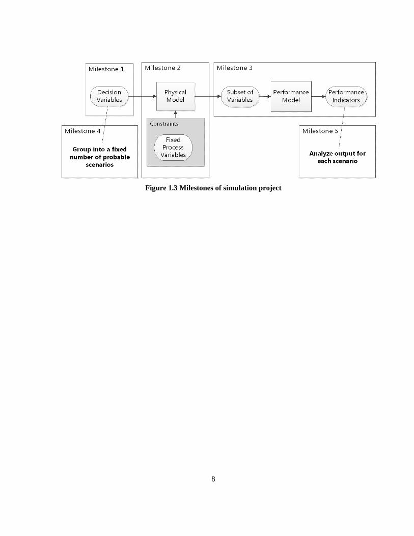
Figure 1.3 Milestones of simulation project
8

1.3 Thesis Scope
The scope of the simulations to be carried out in this is limited by the content of the model: the
components that are represented in the model and their interconnections. In this section, the boundary
of the physical and performance models are outlined.
1.3.1 Physical Model
Figure 1.4 illustrates the interface of the system under consideration, also referred to as the ‘energy
hub’, with its environment. The components of the energy hub and their interactions are modeled
extensively in this project, whereas the environment (power grid, natural gas grid, hydrogen need and
mixture need) are taken to be exogenous parameters. They are described but not modeled
dynamically.
Figure 1.4 Project scope for the physical model
9

1.3.2 Performance Model
The performance model uses some process variables from the physical model and additional model
parameters to evaluate the financial and environmental performance of the energy hub. These two
aspects are evaluated by two separate sub-models: the financial model and the environmental model.
In the end, three types of performance indicators are reported: physical, financial and environmental
(Figure 1.5).
Financially, the performance model evaluates the expected annual cash flow from the operation of the
energy hub, consisting of contribution from the amortized capital cost, fixed and variable operating
and maintenance cost, energy purchases and sales, as well as change in the value of storage inventory
(if applicable). These items are compiled so that the net present value of the energy hub can be
calculated. For simplicity, the performance model assesses the environmental impact of the energy
hub through the accounting of annual carbon dioxide emissions associated with the operation of the
energy hub.
Figure 1.5 Structure of the performance model
The name of the financial model is chosen with care, since there is common confusion between
“economic analysis” and “financial analysis”. The main difference between the two types of analysis
is the scope of analysis, in other words, the boundary of the system under consideration. In an
economic analysis of the energy hub operations, the system to be analyzed would be the energy
10

system of Ontario, in which all provincial suppliers, importers, consumers and exporters of electricity,
natural gas and hydrogen are included. The costs and benefits calculated amount to the total benefits
or costs experienced by the whole province. Meanwhile, a financial analysis is smaller in scope. It
focuses on the costs and benefits for one group of stakeholders – in this project, the operators of the
energy hub – disregarding the benefits and costs experienced by other stakeholders.
The two analysis are complementary: the wider-scoped economic analysis evaluate the overall
benefits of the project to the population involved; whereas the narrower-scoped financial analysis
evaluate whether the incentive of specific stakeholders is adequate for the solvency and longer-term
sustainability of the project. When a project is economically beneficial, but not financially beneficial
to the operators of the project, it is unlikely that the project can be operated sustainably. On the other
hand, if a project is financially beneficial to certain key stakeholders, but costly in the economic
analysis, then the project must be re-examined with care, as it may reveal that some financial benefits
are but transfers between stakeholders.
Scope of Economic Analysis
Scope of Financial Analysis
Stakeholder
Stakeholder
Stakeholder
Stakeholder
Stakeholder
Stakeholder
Figure 1.6 Comparison of economic and financial analysis
11

Chapter 2 Literature Review
This literature review surveys the applications that are commonly attributed to energy storage
technologies and the portfolio of technologies that is currently under research. Then, the features of
the Ontario energy system that are of interest to energy storage are reviewed. Finally, “energy hub”, a
modeling frame work for integrated energy systems is introduced, followed by descriptions of the key
technological components of the UHNG concept.
2.1 Energy Storage
Energy storage is not a specific material or a product. It is a service that is performed to facilitate the
delivery of energy from upstream suppliers to downstream end-users, by providing buffering
capacity. Thus, the suppliers and the end-users do not need to complete their transactions
simultaneously. Overall, the bulk of the energy harvested by human society for specific services
comes from a few primary sources, of which fossil fuels constitute the largest part at 80.9% [12].
Since the primary energy resources typically occur in a location different from that of the energy
demands, we often need to transport them to their final destination, where they are consumed. Except
for cases of continuous transportation through pipelines, the primary energy resources often need to
be stored prior to and after transportation in batches. Then, once distributed to their points of use,
energy resources are also frequently stockpiled, awaiting the time of use.
An energy vector is a form of energy that can be readily transported and stored. Out of all primary
energy sources, only the fossil fuels and biomass can be considered to be energy vectors. Electricity, a
secondary form of energy, is also a transportable energy vector. Since its commercial implementation
in the late 19th century, a wide range of appliances and services has been designed to depend on it.
Thus, as shown in Figure 2.1, a non-negligible portion of fossil fuels and biomass is converted to
electricity.
12

Figure 2.1 Global energy flow for societies [13]
In recent years, electricity is also generated from non-vector primary energy sources such as uranium
(nuclear fission), solar, wind, tidal and geothermal energy. Unlike fossil fuels and biomass, these non-
vector sources cannot be directly used by end-users and are hard to transport. They rely upon
conversion to electricity for transportation and the provision of services, unless distribution of heat is
also feasible.
In a way, electricity is an imperfect energy vector, for, unlike coal or oil, it cannot be readily stored.
The storage of electricity is inherently more complex and less convenient. Typically, electrical energy
cannot be stored directly, requiring conversion to another storable form of energy, the exception
being the case of capacitors. Therefore, historically, the electrical power system was built around one
central tenet: “Electricity must be produced when it is needed and used once it is produced” [1]. The
prevailing operational strategy to maintain electricity supply-demand equilibrium is to reduce demand
through deferrable loads and to adjust supply through dispatchable generators.
13

In the past years, energy storage has attracted increasing academic, industrial and governmental
attention. To understand this new wave of interest, it is necessary to acquire a thorough understanding
of the existing electrical power supply industry, following which the cases of applications of energy
storage could be established.
2.1.1 Electricity Supply Chain
The electric power industry is technically complex. The variety of physical and socio-economic
legacy in which it is grounded led to the development of a variety of forms of ownership, operation
and control. In this section, the various members that participate in the supply chain of electrical
power supply are outlined.
Figure 2.2 Stages in the electricity supply chain
The thick black line in Figure 2.2 represents the flow of electricity. The physical flow is initiated with
energy sourcing, followed by power generation, transportation, supply management (also known as
distribution), metering, consumption, and ends with disposal. Since the consumption of electricity is
relatively clean, generating no waste products, the environment concerns typically associated with
product disposal are not directly applicable. Instead, more attention is paid to the environmental
14

impact of power generation, the stage during which there are significant combustion emissions when
fossil fuels are used.
Market trading is represented by a box by dashed lines, because the market transactions are made
using information about the availability of supply and demand. In Ontario, operators of facilities
connected to the high voltage lines are obligated to participate in the wholesale market: generators,
transmitters, distributors and large loads. Embedded loads, which are not directly connected to the
high voltage lines, are eligible to participate in the wholesale market if their consumption exceeds
250,000 kWh per year. Also, it is possible to participate in market trading without having physical
facilities to generate or consumer electricity: wholesalers, retailers and financial market participants.
The Independent Electricity System Operator (IESO) oversees and coordinates the physical
operations of the system and the financial transactions on the market in real time.
Table 2.1 Typical life cycle of electricity and its participants
Lifecycle Stage Description Participants
Energy Sourcing Harvest energy resource and deliver to the power station
Gas suppliers, uranium suppliers, wind/solar farm operators, hydro-electricity project operators
Power Generation Convert in situ energy supply to electricity, then deliver to transportation infrastructure
Generator operators
Transportation Transmit electricity Transmission network owners
Market Operation Arrange and coordinate energy trading transactions Independent system operators
System Operation Manage the grid to match supply and demand Independent system operators
Market Trading Trade electricity in the competitive market Market participants
Supply Management Sell electricity as a ‘bundled’ product to consumers
Energy retailers, local distributors
Metering Meter the amount of energy consumed and/or traded
Market: all market participants; Residential: local distribution
15

Consumption Consume energy Loads, retail consumers
Disposal and Environmental Impact
Impact predominantly incurred during power generation Generator operators, regulators
As previously mentioned, currently, electricity is produced as it is needed, at all moments. The key
facilitator in the electricity supply chain, who performs the essential coordination between electricity
consumers and suppliers, is the system operator. The system operator has the duties of forecasting the
varying demand for electricity, considering the seasonal and daily factors, and scheduling a large
number of power plants to meet that demand. Based on their economics and dynamic behaviour,
power plants can be divided into three categories:
1. Baseload power plants, which are typically nuclear or coal-fired plants that operate near full
opacity year round; they supply the power that is always needed. In Ontario, baseload power
amounts to about 11,000 MW, supplied mostly by nuclear power generators.
2. Load following power plants, which are intermediate plants used to meet most of the day-to-
day variation in demand. In Ontario, this is supplied by hydro and coal (the latter is to be
phased out by 2014);
3. Peaking power plants, which typically operate only a few hundred hours per year, during the
time of highest demand, often in summer, such as any generation required above 20,000 MW
in Ontario (not visible from figure attached).
16

Figure 2.3 Ontario power generation by type for June 30th, 2013 [14]
In the case that adequate service cannot be provided by the regular generators, additional power
plants under special contracts are brought on-line to restore reliable power supply. The generators on
call to replace normal supply in case of equipment failures or emergencies are known as the operating
reserve. Operating reserve generators are contracted for their ability to supply power on demand; they
receive payment even when actual energy service is not invoked. They can be either spinning or
supplemental; spinning reserves are units that are partially loaded or highly responsive. Generators
which can be restarted without outside source of power (black-start capability), generators which vary
their output automatically, within seconds or minutes, in response to signals sent by the IESO
(regulation service), and generators that are able to adsorb and generate reactive power (reactive
support and voltage control) are known as ancillary services, which are contracted by the system
operator to ensure system reliability for all users of the grid.
Energy storage is considered to be one of the methods that can be used to match supply with demand;
the others include traditional load following, spinning reserve plants and demand-side management.
2
0K5K10K15K
ComponentOTHER TotalGAS TotalWIND TotalCOAL TotalHYDRO TotalNUCLEAR Total
ComponentOTHER TotalGAS TotalWIND TotalCOAL TotalHYDRO TotalNUCLEAR Total
17

Whether energy storage is deployed, depends on its economics compared to other alternatives to
provide grid balancing services.
2.1.2 Applications of Storage in the Existing Grid
It is believed that in historical studies, the economic benefits of energy storage have not been properly
accounted for. This is due to the simplistic assessment method used and the difficulty to quantify the
various values streams generated by energy storage. In this section, the various applications of energy
storage are grouped according to the location of the energy storage facility in the existing electricity
supply chain. The location of the energy storage facility has implications on its ownership and
operating philosophy. The stage of resources extraction is absent, because by then, energy is still in a
pre-electricity form (fossil fuels, uranium, heat, wind, etc.), therefore beyond the scope of electrical
energy storage.
2.1.2.1 Located Near and Operated by Power Generators
For baseload generators, such as nuclear power plants, changes in power output according to
dispatches are possible but undesirable, because plant equilibrium takes a long time to establish or
other operational requirements limit such adjustments. The economics of such plants typically
improve with the higher power plant utilization factor; therefore, they are used to provide more or less
constant power near their generation capacity throughout the year. Occasionally, during off-peak
hours, the output from baseload power plants exceeds the demand on the grid and causes negative
electricity pricing.
Generation shifting for baseload power is the practice of charging an energy storage device using the
low cost baseload power during off-peak hours, saving it for dispatch when market demand is higher.
Here, it is assumed that the storage technology is operated by the baseload power supplier. From this
perspective, an energy storage project will be economically attractive if the decreased O&M costs due
to higher capacity utilization and increased revenue from shifting time of transaction are higher than
the costs of implementation.
18

Figure 2.4 Conceptual diagram for baseload power generation shifting
In additional to the aforementioned benefits, from the system operator’s perspective, generation
shifting may decreases the cost of power that must be produced to meet demand during on-peak
hours, given that lower-cost power from baseload generators are moved to replace some of the output
from load-following and peaking power plants. If the power output provided by energy storage
facilities is large enough, it may even be able to defer the construction of more load-following and
peaking plants. A more comprehensive economic analysis would compare the economic costs and
benefits of the case with and without energy storage, for the scope indicated in Figure 2.5. The price-
setting mechanism within the wholesale electricity market will need to be included in the analysis, if
the power drawn and delivered by the energy storage facility is deemed large enough to influence the
market-clearing price.
19

Figure 2.5 Scope of analysis for generation shifting
2.1.2.2 Located Near Transmission Network and Independently Operated
Currently, the transmission and distribution facilities of a power system are built to serve the peak
demand, so the lines must be expanded at the same rate as the peak demand, regardless of under-
usage during off-peak hours. In Ontario, the high capital costs of the under-used T&D network are
borne by all market participants via the payment of Wholesale Transmission Charges. Given that grid
demands are now met instantaneously with transmitted supply, it has been impossible to justify
transmission networks which are sized below the peak demand.
In this context, energy storage can be used to relief network congestion, decreasing the need for
expansion in transmission capabilities, and allowing the grid to operate with transmission lines which
are sized below peak demand. It achieves this by allowing charging and discharging of power
independent of transmission network congestion.
20

Located downstream of points of grid congestion, the energy storage facility can proceed to charging
when the lines are not congested, then deliver that energy downstream during periods of congestion.
Figure 2.6 is only a much simplified version of the real scope of analysis; a complete analysis for this
type of application must take into account the geographically disaggregated nature of power
transmission lines, power generators and power loads. An energy storage facility would be preferred
if it successfully alleviates grid congestion with costs lower than that of alternatives (expansion and
construction of new power lines).
Figure 2.6 Scope of analysis for grid congestion relief
2.1.2.3 Other Applications for Independently Operated Storage
The restructuring of the electricity wholesale market has also created a market for ancillary services
that energy storage facility operators can participate in. In Ontario, the ancillary services that the
IESO contracts on the procurement market are certified black start facilities1, regulation service2,
1 Certified Black Start Facilities are able to restart their generation facility with no outside source of power. 2 Regulation Service corrects variation sin power system frequency by responding to IESO signals with response times ranging from tens of seconds to a few minutes.
21

reactive support and voltage control service3. Operating reserve contracts, requiring response of
generators within 10 to 30 minutes of activation, are also available.
2.1.2.4 Located Near and Operated by Energy End-Users
Energy end-users can sometimes use energy storage for energy cost reduction. Currently, many
utilities have implemented a power tariff that varies based on the time of use. In this case, energy
storage could be used to shift demand from periods with high prices to those with lower prices. This
is comparable to generation-shifting by power suppliers. There exists the difference that the small
volume power end-user makes charging and discharging decisions based on energy retail price,
whereas power suppliers base their decisions on energy wholesale market price. Some industrial and
commercial customers, which are large volume end-users, pay a demand factor-based tariff which
varies with the time of use and the amount of power used. In other words, they also participate in the
energy wholesale market. Energy storage can help them spread out their peak demand over a longer
period of time, thus reducing the costs of energy.
If the end-users have devices or equipment highly sensitive to voltage or frequency deviation, they
will benefit from energy storage for improved reliability. Energy storage facilities will buffer
imbalances between the local demand and the supply from the grid, keeping frequency and voltage at
the nominal value. Energy storage is equally beneficial to customers who are concerned with power
supply disruption. Near the end of the supply chain, the flow of power tends to be smaller, and the
scope of the cost and benefits study, also smaller.
3 Reactive Support and Voltage Control Service are reimbursement to dispatchable generating facilities which incurred additional costs to provide reactive support/voltage control services.
22

Figure 2.7 Scope of analysis for end-use energy reliability and cost reduction
2.1.3 Applications of Storage in the Future Grid
For intermittent power generators, such as wind turbines and run-of-the-river hydro generators, their
source of energy can at best be forecasted, let alone varying their output at will. From a RE generator
operator’s perspective, the viability of RE projects, is hindered by their lack of control over the time
of power generation once governmental subventions are removed. Power from renewable sources
must be sent to the grid as it is produced, without consideration of market supply and demand.
Energy storage technology could improve RE projects profitability by making their intermittent
power output predictable and dispatchable. Operated by RE project operators (Various commercial
firms in Ontario), energy storage will enable RE generators to compete on an equal basis as
conventional, often fossil-fuel-based dispatchable generators. Depending on the scale of storage, part
or all of the fluctuating power generated could be consolidated and dispatched according to the
instructions of the system operator, as power is needed. This is expected to increase the revenues of
RE project operators.
23

Once the penetration of RE projects has crossed a critical threshold, beyond which significant power
variability control is required. Figure 2.8 shows how, with a high wind penetration (>20%), currently
small fluctuations in power output could be amplified and place even more requirement on
conventional generators used for load following. By 2018, the non-hydro renewable energy
generating capacity is expected to expand to 10,700 [15]. In the year 2012, most of the non-hydro
renewable energy generating capacity in Ontario comes from wind power. It would need to be
increased by seven times, if the Supply Mix Directive of the Ontario Ministry of Energy were to be
followed. A hypothetical scenario in which the wind power levels in Ontario increases by ten-fold is
shown in Figure 2.8.
From a system operator’s point of view, the intermittency and unpredictability in their power output
will become increasingly problematic, as the percentage of renewable energy (RE) generators in a
grid’s supply mix increases. The increasing fluctuations will need to be countered by the installation
of more dispatchable generators (i.e. gas-fired generators). This problem is believed to be significant
once RE penetration exceeds 20% of the total supply mix [16]. For lower penetration, the variability
in wind power output is smoothed by the aggregation of multiple geographically-dispersed sources.
By that time, in order to ensure the reliability of the grid, supply variability from individual power
supplier might be discouraged with penalty charges (which do not exist as of now). They may then
choose to operate an energy storage technology of appropriate scale to release power in a controlled
manner. The system operator could also manage supply variability caused by RE project centrally,
by adopting a larger-scale energy storage technology capable of smoothing the aggregated supply
from multiple RE generators.
On the side of supply, because some of the RE resources are found in remote locations, new
transmission lines and expansion of existing lines are often needed to connect them to the point of
use. The sizing of those new transmission and expansion projects reveals a dilemma: the lines could
be sized to accommodate the peaks in RE production, remaining under-used during off-peak hours.
They could also be sized for the typical flow throughout the day, cutting off the supply of RE power
once the lines have reached full-capacity during peak hours. The first approach has high capital costs,
which are eventually borne by all ratepayers as delivery fees; the second approach result in
24

constrained-on and constrained-off payments which are charged as overheads to the participants of
the real-time wholesale electricity market.
Figure 2.8 Hypothetical weekly grid supply scenario with high wind power penetration
0
5000
10000
15000
20000
25000
Pow
er (M
W)
Ontario DemandWind CurrentWind FutureLoad on Conventional Generators
25

2.1.4 Conventional Energy Storage Technologies
The applications that a given energy storage facility can perform is dependent on the amount of
energy that it can store, its response time and the rate at which the energy can be released or stored.
The Electric Power Research Institute has published their findings on the scale of energy storage
system required for different applications (Figure 2.10). It can be seen that, despite of some small
overlaps in between applications, most applications are not simultaneously compatible. Those
interested in a particular application of energy storage need to select an energy storage technology
that is able to perform within the ranges prescribed by the given application.
Figure 2.9 Operational benefits monetizing the value of energy storage [10]
The following section provides a survey of the different methods of bulk energy storage currently
available or under active development. The technologies typically proposed for grid energy storage
are batteries, compressed air energy storage (CAES), pumped hydro energy storage, advanced
capacitors, flywheel energy storage, superconducting magnetic energy storage, and energy storage
through hydrogen [6-11]. Because energy storage through hydrogen is still at a conceptual stage and
will be the main focus of this project, it is discussed in an independent section following the literature
review.
26

Vehicle-to-grid (V2G), a system in which electric vehicles act as distributed energy storage devices
has also been proposed [11]. However, the deployment of V2G at utility scale requires the
participation of individual consumers, through the purchase and use of plug-in hybrid electric
vehicles (PHEVs). This is subject to many socio-technological impediments[17]. Therefore, the V2G
concept is not addressed as part of this literature review.
When describing each energy storage system, the fundamental principle of its operation, the system
components, and its stage of development are outlined. Then, in order to achieve meaningful
comparison, a fixed set of properties is introduced for each alternative and compared whenever
possible. The selected properties are:
Round trip efficiency, defined here as the percentage of electricity sent for storage which can be
recovered as electricity. The technology with the highest round trip efficiency is more favorable,
because low efficiency, implying that only a fraction of the energy stored can be retrieved, increases
cost of storage per unit of retrievable energy.
Storage capacity and rated power, determined by the energy and power densities of the storage
devices. Together, these two properties determine the field of application of the energy storage
technology. Storage capacity is the maximum amount of energy that a storage device can hold, and
rated power determines at what rate the stored energy could be recovered. For energy storage at
utility-scale, especially when storing off-peak excess power for later use, it is desirable for the energy
storage unit to store several thousand MWh of energy, and release at rated power above several
hundreds of MW [18].
Storage timescale, representing the time period for which energy can be stored using the technology,
taking into account phenomena such as self-discharging. Since load placed on the power grid varies
by time of day and by season, it is desirable for the chosen technology to be able to store energy for
several hours, even up to months, without degradation.
Durability of equipment is represented by the number of charge-discharge cycles that the system can
undergo without refurbishment or replacement. A short lifespan is undesirable, because it increases
the costs of storage in the long term by multiplying the costs of replacement.
27

Cost of storage is a parameter that measures the economic competitiveness of the technology. It
varies depending on the stage of development and the nature of a given technology. The values
presented in this section are costs for the total energy storage system per unit of energy stored,
whenever available. Since this is an exploratory project that simulates a future scenario, the cost is
only given as indicators, not as a criterion. This ensures that options are not discarded purely by costs,
for development following the current research will be able to affect future economics.
Other characteristics of a technology, such as geographic requirement or auxiliary equipment
requirement are noted whenever applicable. They will be used to further refine the choice of a large-
scale energy storage technology.
2.1.4.1 Battery Systems
All battery systems convert electrical energy to chemical energy for storage. When charging, an
electrical potential is applied and the batteries undergo an internal chemical reaction. The discharge of
stored energy occurs when the chemical reaction is reversed. The types of batteries listed below
mainly differ by the material used for the electrodes and the electrolyte, since different chemical
reactions are involved. Note that, since the electrodes in these batteries participate in the chemical
reaction and store the products via solid state reactions, the energy and power densities of the battery
are dependent on the size and geometry of the electrodes [6]. Also, most of them have lifetimes which
are affected by operating conditions such as depth of discharge, operating temperature and fast
charge/discharge cycling ([1]. Since batteries are direct current (DC) systems, a power conversion
unit is required for them to interface with the grid, where energy is generated and transmitted as
alternating current (AC).
2.1.4.1.1 Lead-Acid Batteries
The lead-acid battery is a very mature and established technology. It uses elemental lead as anode and
lead dioxide as cathode; the electrodes are immersed in a dilute sulfuric acid. The round trip
efficiency of a lead-acid system ranges from 70% to 80% [11]. Typical energy density values are
about 30 Wh/kg, and the total stored energy can be discharged in tens of minutes to an hour [8], so 28

the power density is estimated to be around 150 W/kg. Because there is very little self-discharge (2%
of rated capacity per month), lead-acid batteries are appropriate for long term storage. Currently, such
systems are expected to last from 1000 to 2000 charge/discharge cycles at 70 % depth of discharge [9,
19]. Storage cost per installed storage capacity is $425-475/kWh, and relatively little maintenance is
needed [10]. But, because of the maturity of the technology, no significant breakthrough is expected
with respect to system lifetime and costs[9]. Lead-acid batteries are commonly used when low energy
density is acceptable and high abuse tolerance is required, in applications such as automotive starting,
lighting and ignition, and battery-powered uninterruptible power supply. The disposal of a large-scale
lead-acid system causes environmental concern, for it contains a toxic heavy metal.
2.1.4.1.2 Nickel-Cadmium Batteries
A nickel-cadmium battery (Ni-Cd) consists of a cathode made of nickel hydroxide, anode made from
metallic cadmium, with an aqueous potassium hydroxide solution as electrolyte [11]. Energy and
power density ratings for this type of battery are 40-60 Wh/kg and 140-180 W/kg, with a round-trip
efficiency of 60-90%. At 10% of rated capacity per month, the self –discharge rate is higher than that
of lead-acid batteries, but still acceptable for hour-long storage purposes[8]. A Ni-Cd system has
durability estimates of 1000-2500 charge/discharge cycles and 10-20 years, and is more durable than
lead-acid batteries at higher operation temperatures [1, 9], The storage cost per installed capacity is
$1000-2000/kWh, more expensive than that of lead-acid systems. One important disadvantage of the
Ni-Cd battery is the toxicity of cadmium, which will require a complex recycling procedure if
deployed, to minimize negative environmental impacts.
2.1.4.1.3 Sodium Sulfur Batteries
Sodium sulfur batteries (Na-S) has molten sulfur at the cathode and molten sodium at the anode; the
two electrodes are separated by a solid beta alumina ceramic electrolyte, which only allow positive
sodium ion to pass through [7]. The literature reports round-trip efficiency of around 75% [10]. Na-S
batteries have energy density of 120 Wh/kg, and power density of 120 W/kg [11], Since there’s no
noticeable degradation of stored energy through self-discharge, long-term storage using Na-S
batteries is very favourable [19]. At 100% discharge, a Na-S battery can last up to 2500 cycles; its
lifetime is further extended at shallow depth of discharge (40,000 cycles at 20% depth of 29

discharge)[1]. Cost-wise, most recent values for large-scale applications are $520-550/kWh [10].
Both sodium and sulfur are abundant low-cost material, making the battery suitable for mass
production. The battery operates with molten compounds; therefore, the operating temperature, about
300 °C is much higher than the ambient temperature and requires heating in stand-by mode [19]. The
auxiliary heating requirement places a parasitic load on the overall system and reduces its efficiency
[7]. They have been used for load leveling, emergency power supply or UPS.
2.1.4.1.4 Lithium-Ion Batteries
Lithium ion batteries (Li-Ion), known to the public through their wide use to power portable
equipment, laptops, cameras, cell phones and portable tools, are made up of lithiated metal oxide
cathodes and graphitic carbon anodes with layer structure. Lithium salts dissolved in organic
carbonates act as the electrolyte [7]. Very high round-trip efficiency has been reported for Li-Ion
batteries: 87-92% [10]; energy and power densities are 100-200 Wh/kg and 360 W/kg, respectively
[11]. Self-discharge occurs at the rate of 5% of rated power per month [8]. In its lifetime, the Li-Ion
battery is able to complete more than 1500 charge/discharge cycles, 3000 cycles at 80% DOD [19].
The main obstacle to large-scale applications of Li-Ion batteries is its higher cost: $1500-3500/kWh
[9]. Because of its high energy density, Li-Ion batteries are studied for use in plug-in hybrid and
electrical vehicles.
2.1.4.1.5 Flow Batteries
As aforementioned, the electrodes of most batteries participate in storage, tying the energy and power
densities of a system to the electrodes’ size and shape. One exception exists: flow batteries. Flow
batteries consist of two liquid electrolytes in an electrochemical cell with two compartments,
physically separated by an ion-exchange membrane which only selected ions can pass through. In
this case, the system is easily scalable, since the storage capacity is set by the electrolyte tank
capacity, and the rated power, by the electrolyte flow rate and the area of the membrane [11].
There are three types of flow batteries: vanadium redox (VRB), polysulfide bromide (PSB) and zinc
bromide (ZnBR). Of the three, VRB uses compounds of vanadium in both electrolyte tanks,
30

eliminating cross contamination of electrolytes, allowing for easy recycling [7]. It has also shown a
longer lifetime and is more developed than the other two types of flow batteries. Therefore, VRB is
used to represent flow batteries in general in this review of technologies.
Round-trip efficiency of VRB, also called AC to AC efficiency, is about 75% [9]. Energy density per
mass of electrolyte is 25 Wh/kg and power density is 80-150 W/kg [11]. The battery can be fully
discharged without adverse effects, and self-charge is negligible since little electrolyte is lost over
time, encouraging its use for long term storage applications [7]. Lifetime is estimated to be 1000-2500
charge/discharge cycles, or 10 years [9]. Finally, by economy of scale, the storage cost per installed
capacity decreases as the system size increases, $620-740$/kWh are the most recent values derived
from calculations for a 250 MWh demo facility [10].
2.1.4.2 Flywheels
Flywheels convert electrical energy to kinetic energy for storage, in the form of a mass rotating about
an axis. To charge the flywheel, a motor is used to accelerate the flywheel; for retrieval, the flywheel
is slowed down via a decelerating torque to the motor, now reversely used as a generator [8]. The
energy stored is a function of the moment of inertia of the rotor, and the square of its rotational
velocity. Low speed flywheels are typically made of steel and high speed flywheels (>50,000 RPM)
are made from composite materials. Containment vessels are required to deal with potential rotor
failures. Magnetic bearings and vacuum chambers are sometimes used to reduce losses from friction
[6].
The roundtrip efficiency of such systems is high for short periods of storage: 90% [9]. However,
flywheels have very high standing losses. After five hours of storage, the overall efficiency is reduced
to 78%, and 45% after one day [18]. In some instances, up to 20% of stored capacity could be lost per
hour for non-continuous cycling [8]. Therefore, long term storage is not foreseeable with this
technology. As for storage capacity, low speed flywheels have energy density between 5-30 Wh/kg,
while high speed flywheels have ratings higher than 50 Wh/kg [11]. Flywheels have extremely high
power density: 1000 W/kg for low speed flywheels and 5000 W/kg for high speed ones, although the
peak power rating does depend on the power ratings of the power converter and the motor/generator.
31

Within the lifetime of one flywheel, it can support more than 100,000 complete charge/discharge
cycles, operating for 10 years and longer [9].
Costs for flywheel storage are more reasonable when compared to other technologies on a storage
cost per installed power capacity ($/kW) basis, not as cost per installed energy capacity ($/kWh). The
per power value, ~$2000/kW compares well to other storage options, which mostly have values that
range from $1000/kW to $5000/kW. But, the per energy value, $7800-$8800/kWh, is the highest
among all existing options [10]. In other words, flywheels are not strong candidates for bulk energy
storage, but are more suitable for power quality control applications which require high power
delivery over short period of time.
2.1.4.3 Advanced Capacitors
Three types of advanced exist: electrochemical double layer supercapacitors (ECDL),
pseudocapacitors, and hybrid capacitors. Out of the three, ECDL is the most fully developed and will
be the focus of this review. Capacitors store energy by physically separating positive and negative
charges with an insulating dielectric. In supercapacitors, the insulating material is replaced by an
ionic electrolyte, in which conducting electrodes are submerged. When charging, the voltage applied
creates an electric field that enables the ions in electrolyte to migrate towards electrodes of opposite
polarity, forming an electrostatic electrical equilibrium at the surface of electrodes. The capacitance
of supercapacitors is much larger than regular capacitors, because the separation of charge occurs at
much smaller distances, and because electrodes are made of porous carbon with very large surface
area [8].
Since the separation of charge is physical rather than chemical, the effect is easily reversible, leading
to high efficiency such as 95% [11]. For the same reason, the rate of charge and discharge is faster
than that of batteries, operating based on chemical reactions. ECDLs are capable of delivering 4000
W/kg, potentially 100,000 W/kg if electrodes are made of carbon nanotubes. Energy density is close
to 5 Wh/kg, with hope of attaining 69 Wh/kg when carbon nanotube electrodes are used [8].
Supercapacitors have high self-discharge rate: about 14% of nominal energy is lost per month. The
nature of energy storage in supercapacitors implies that degradation is minimal for deep discharge
and over charge. A lifetime of 400,000 cycles at 100% depth of discharge is expected. Because of
32

their low energy density, investments per installed capacity for ECDLs are very high, around
$20,000/kWh [8]. Overall, supercapacitors are more suitable for high peak-power, low-energy
situations.
2.1.4.4 Superconducting Magnetic Energy Storage (SMES)
SMES stores energy in the magnetic field generated by DC current flowing through a
superconducting coil. The operation mode of the superconducting coil is controlled by altering the
voltage across the coil. Positive voltage charges the coil and negative voltage leads to discharge. In
standby mode, there’s no voltage difference across the coil. Because the superconductor needs to be
maintained below its superconducting critical temperature, the SMES system needs a cryogenic
cooling system, in addition to the power conversion/conditioning system and the coil [6].
The charge-discharge cycle of SMES systems can reach instantaneous efficiency of more than 95%
[18]. The storage capacity of a superconducting coil is dependent on its size and temperature, among
other properties. These units can respond to change of mode within a few milliseconds, then provide
very high power output, but only for a very short while [1]. They are able to complete a great number
of charge-discharge cycles at 100% DOD. In between charging and discharging, SMES systems have
a small power loss in the non-superconducting part of the circuit, so a small trickle charge is
necessary to replace the lost power. This is comparable to self-discharge in battery systems.
Large SMES projects might need to be contained underground in order to shield the effect of the
enormous electromagnetic forces that are generated [18]. As with supercapacitors, SMES systems
have competitive storage costs per installed power, but much higher storage costs per installed energy
storage capacity. For example, for a hypothetical 100 MW, 500 kWh SMES project, the costs are
$1970/kW and $394,000/kWh [20].
2.1.4.5 Compressed Air Energy Storage (CAES)
Conventional gas turbines consume up to two-thirds of the fuel used to compress air, before directing
it to the combustor for combustion with fuel [6]. To compress the air needed by gas turbines, CAES
systems use compressors powered by off-peak electricity instead more expensive natural gas.
Compressed air can be stored in vessels, but the pressure that tanks can withstand limits the storage 33

capacity of this technology. Therefore, in for large-scale applications that absorb grid excess power,
the compressed air is stored in underground mines, caverns or aquifers. A complete CAES system
comprises of motors/generators, compressors, expansion turbines, an underground formation for
storage and auxiliary equipment. Before being injected underground, air is cooled and pressurized.
When it is extracted from storage, it must first be preheated in a recuperator before being mixed with
gas to be combusted and expanded in the turbines [8]. There are three types of CAES technologies
based on how heat exchange is managed for compression: isothermally, adiabatically or diabatically
[11]. Isothermal systems allow the temperature to equalize with the surroundings by slow
compression, thus limiting power delivery rate, is more suitable for small-scale projects. Adiabatic
systems store heat released during compression for later use in the recuperator, requiring a heat-
storing device. Diabatic systems use external energy to heat or cool air throughout the process and are
most common.
The round trip efficiency of existing diabatic systems in operation is about 50%, lower than that of
proposed adiabatic systems, 75% [9, 21]. CAES technology is typically used for very large-scale
storage projects, having rather low energy density of between 10-30 Wh/kg [11]. The rate at which
power can be delivered using CAES technology is dependent on the output specifications of the
combustion turbines into which the compressed gas is fed. To recover energy stored, a combustion
turbine power plant fitted with CAES is able to start-up rapidly in 9 to 12 minutes, compared to the
required 20-30 minutes of conventional combustion turbine peaking plants [8]. The energy can be
stored for more than a year, since losses are very small. A CAES project can have lifetime of more
than 20 years, or more than 5000 cycles [9, 11], and the most recent storage costs per installed
capacity is $60-120/kWh [10]. The obvious limitations of CAES technology are the requirement of
an adequate underground storage facility and its dependence on an on-site combustion turbine power
plant for energy recovery.
2.1.4.6 Pumped Hydro
Pumped hydro stores energy by circulating water between two reservoirs with a height difference. To
charge the system, water is pumped from the lower reservoir to the upper reservoir, consuming
power; to discharge, water stored by the upper reservoir is released and flow into the lower one
through a turbine, generating power. The typical components of such a system are: reservoirs with
34

appreciable hydraulic head, connected through a set of reversible pumps/turbines [8]. Both freshwater
and seawater systems exist, with the open sea being the lower reservoir. Sometimes, well-located
abandoned mines can also act as the lower reservoir.
The overall efficiency of pumped hydro operations were 60% in their beginnings in the 1960s,
currently, more recent values of about 80% are reported [7, 9, 11]. The losses mainly come from
evaporation at exposed water surface and from energy conversion at pumps and turbines. The energy
density for pumped water storage is very low (0.3 Wh/kg). Therefore, small-sized projects are rarely
economical. The storage capacity of the technology is dependent on the body of water available and
on the variation in height between the two reservoirs. The response time of a pumped hydro plant is
on the order of seconds, like other conventional hydroelectric plants. Only 10 to 30 seconds is
required for the plant to ramp up to full power from standby mode, and 10 minutes are needed to
switch from complete shutdown to full power mode [1]. The self-discharge of this technology is
negligible, and its lifetime, measured in decades, is from 20 to 50 years [9]. System development
costs for pumped hydro projects are notably high, in the range of $420-430 for 280 to 530 MW
facilities, and $250-270 for 90 to 1400 MW facilities [10].
Pumped hydro is the oldest and largest of all commercially available energy storage technologies. In
2010, more than 99% of the world’s installed energy storage capacity (127,841 MW) consists of
pumped hydro energy storage. However, most of the easily exploitable operating sites have already
been taken. The interest in pumped hydro waned after the 1980s, because of high capital costs and the
difficulty in locating new operating sites [1]. Efforts in this field are now directed toward upgrading
existing projects rather than launching new ones.
35

Figure 2.10 Energy storage technologies by power ratings and discharge time [10]
36

Table 2.2 Summary of existing energy storage technology benchmark parameters [6]-[20].
Technology
Option
Efficiency Energy
Density
Power Density Self-Discharge
Rate
Durability Cost of Storage Geologic
Requirement
AC-to-AC Wh/kg W/kg capacity per day cycles $/kWh installed
Pb-Acid Battery 70-80% 30 150 0.1% 1000-2000 425-475 No
Ni-Cd Battery 60-90% 40-60 140-180 0.3% 1000-2500 1000-2000 No
Na-S Battery 75% 120 120 0.0% 2500 520-550 No
Li-Ion Battery 87-92% 100-200 360 0.2% 1500-3000 1500-3500 No
VRB 75% 25 80-150 0.0% 1000-2500 620-740 No
Flywheels 90% 5-30 OR 501 1000 OR 50001 45.0% 100,000 7800-8800 No
ECDL Capacitors 95% 5 4000 0.5% 400,000 20,000 No
SMES 95% low to moderate very high very low -- 394,000 Sometimes
CAES 50% 10-30 N/A N/A >5000 60-120 Yes
Pumped Hydro 80% 0.3 N/A N/A >10,000 420-430 OR 250-2702 Yes 1 The lower energy/power density values are for low-speed steel flywheels, and the other one, high-speed composite flywheels 2 The lower cost values are for pumped hydro projects with rated power > 900 MW
37

2.2 The Case for Ontario
As of 2012, Ontario has over 34,000 MW of installed generation capacity. The breakdown of
Ontario’s generating capacity is shown by Figure 2.12.
Figure 2.11 Ontario’s installed generation capacity by type [22]
The real percentage of demand met by each type of energy supply differs from their percentage in the
installed generation capacity. Because, the actual amount of generation actually available at any given
time is dependent on outages and the capacity factor of each forms of supply. Power could also be
imported from neighbouring jurisdictions. The actual use of energy by type of supply for the past few
years are shown by Figure 2.13. We observe nuclear power to be the most important source of power
supply at 55%. Some other trends could also be summarized from this figure: coal’s share is
decreasing, gradually replaced by natural gas; also growing is the power generation by wind, albeit a
very small percentage of the total power output.
Nuclear 33.2%
Gas 28.9%
Coal 10.2%
Hydro 23.0%
Wind 4.4%
Other 0.4%
38

Figure 2.12 Total electricity output by fuel type [2]
In October 2012, two units at the Bruce Nuclear Facility with a combined capacity of 1500 MW have
been restarted, achieving commercial operation after being shut down for 17 years. This further
increases the installed capacity of nuclear power, which is conducive to surplus baseload generation
conditions, until the refurbishment of the Darlington units (3800 MW) between 2016 to 2024 and the
retirement of the Pickering nuclear units occur in 2020 ([23]). Meanwhile, aligned with the Supply
Mix Directive issued by the Ministry of Energy of Ontario in February of 2011, non-hydro renewable
power generators (wind, solar and bio-energy) are expected to increase their installed capacity to
10,700 MW in 2018, representing 10-15 % of total Ontario electricity generation [15].
The combined effect of increasing RE generators (mostly wind turbines) and plentiful baseload power
supplied by nuclear power plants has already influenced Ontario’s wholesale electricity market.
Today, the wholesale electricity market is the mechanism through which electricity supply and
demand in the province is balanced in real-time. In addition to the system and market operator (the
IESO in Ontario), market participants come from all stages of the electricity life cycle: generators,
distributors, electricity retailers, etc. Mandated to oversee Ontario’s wholesale electricity market, the
IESO administers a set of rules that govern the transactions of all the market participants, by
authorizing market participants, publishing load forecasts and market information, producing
statements and invoices, and performing financial settlement transactions.
0%
10%
20%
30%
40%
50%
60%
Nuclear Hydro Coal Gas Wind Other
2008
2009
2010
2011
39

One of its most important duties is to set the commodity price for electricity based on market
conditions. Every five minutes, the IESO calculates the market clearing price, taking into
consideration information submitted by all market participants: generation schedules, bids and offers
to generate or purchase energy at different price points. Every hour, the Hourly Ontario Energy Price
(HOEP) is determined by the average of the five-minute prices; it is the price applied to the non-
dispatchable generators and loads; whereas dispatchable generators and loads make transactions at the
five-minute real-time price.
Since 2007, the HOEP have dipped into the negative for increasing number of hours (Figure 2.14), for
during those hours, the supply of electricity generated by the non-dispatchable generators has
surpassed the provincial demand for electricity. Such a market signal has initiated a conversation
about the implementation of energy storage technology in the province.
Figure 2.13 Number of hour per month with negative HOEP [14]
2007
020406080100120140160
40

2.3 Energy Hub Framework
Since 2002, the project “Vision of Future Energy Networks”, undertaken by researchers at the Swiss
Federal Institute of Technology (ETH) Zurich, has produced a series of publications that focus on
general system modeling framework for future energy networks. The development of such modeling
frameworks are motivated by the challenges that the electric power infrastructure faces: aging assets
approaching the end of their lifetime, requiring replacement; growing use of natural gas to supply
combined-cycle turbines for power generation, increasing the coupling between the power and gas
networks, while the supply of fossil fuels remains finite and uncertain; and the integration of small
and distributed energy sources, sometimes involving several energy carriers. It is hoped that, using
the modeling frameworks developed, the optimal system structure and operation strategies for future
energy networks can be determined. The transition paths that bridge today’s system with the future
optimum can then be identified.
Three key concepts have emerged from their work: energy hubs is a modeling frameworks that can be
extended or customized for modeling, analysis and planning of energy system scenarios.
2.3.1 Definition
An energy hub is an integrated system of units which is able to condition, convert and store multiple
energy carriers. As illustrated by Figure 2.15, within an energy hub, there are several units that can
convert or condition incoming energy carriers, so that the local load can be met. In other words,
energy hubs can be viewed as interfaces between energy consumers, energy producers and the
transmission infrastructure; equipped to store or convert in between energy carriers if necessary.
Energy hubs allow connected consumers to access energy in the form that they desire, at the time that
they desire, which may be different from the form or time in which energy supply is delivered to the
hubs.
41

Figure 2.14 Generic schematic of an energy hub [24]
2.3.2 Methodology
There are three types of elements within an energy hub: converting units, conditioning units and
storage units, and they are represented differently mathematically. The section above briefly outlines
the “energy hub” approach developed by the research group at ETH.
The converters and conditioning units in the energy hub are abstracted and simplified to a level
appropriate for analysis. So, it is assumed that they can be characterized by their efficiencies. In the
case of multiple inputs and multiple outputs, the relationship between conversion/conditioning
efficiency, energy input, energy output and different forms of energy carriers is represented by the
coupling matrix C, which balances the input and output power flows [25]:
PL c c c P
c c cL
c c c PL
α αα βα ωα α
αβ ββ ωβ ββ
αω βω ωωω ω
=
PL C
(2.1)
The vector P contains all values of energy inputs to the converters/conditioning units, and the vector
P, all values of load placed on them; the set of energy carriers are denoted by small Greek letters α to
ω. When the two subscript letters differ, the energy transaction taking place is a conversion process;
when they are identical, the energy transaction taking place is a conditioning process, i.e. no change
in energy carrier has occurred.
To account for the splitting of input among several type of converters (e.g. not all of Pα is
transmitted/converted through one type of conversion units; instead, it is distributed to feed different
42

converters that transform energy vector α to several energy vectors), dispatch factors v are introduced
to specify the input flow associated with a particular conversion. For converter κ, for example:
P v Pακ ακ α= (2.2)
The entries of the coupling matrix represent the efficiencies of particular conversion; they can be
constants or functions of the power flow through the unit, with values ranging between 0 to 100%.
Storage devices in energy hubs are conceptualized as an ideal storage equipped with an interface for
energy exchange. Therefore, in addition to being characterized by conversion efficiency, as a
converter, a storage device is also characterized by its energy content: the amount of energy that is in
storage. At the interface, the storage device is modeled as follows:
Q e Qα α α= (2.3)
Where: Qα is the power flow to the storage device, Qα is the power flow that has been converted into
the form of the storage medium, also known as the internal power flow, and eα is the
charging/discharging efficiency, depending on the direction of power flow. Similar to conversion
efficiency, charging and discharging efficiency values can be constants, or function of another
variable.
if 0 (charging/standby)
1 else (discharging)
e Qe
eα α
αα
+
−
≥=
(2.4)
The energy that is in storage is the integral of the power flow over time, with a given initial value. Or,
in other terms, the internal power flow is the time derivative of the stored energy. In this framework,
it is assumed that the flow of power Qα can be approximated to be constant during the time step t∆
( ) ( ) ( )0
0T
E T E Q t dtα α α= + ∫ (2.5)
dE EQ Edt t
α αα α
∆= ≈
∆
(2.6)
The subsequent combination of storage devices with converter elements is dependent on the location
of storage within the energy hub: connected to the input energy carriers, the output energy carriers, or
between the two sets of energy carriers.
43

Figure 2.15 Storage elements in energy hubs [25]
Storage elements connected to the input energy carriers divert power from the input Pα , while storage
elements connected to the output energy carriers divert from converted power Lβ
P P Qα α α= − (2.7)
L L Mβ β β= + (2.8)
In the shaded area in Figure 2.16 Storage elements in energy hubs [25], there are no storage element
connections. Thus, the energy hub elements within can be described using the converter-only model
in equation(2.1). The effect of storage flows can be added to this original equation through the
following manipulation:
( )L + M = C P -Q (2.9)
( )L = C P -Q - M (2.10)
eqL = CP - CQ - M = CP - M (2.11)
The equivalent storage flow vector eqM is related to the approximated internal power flow E
through the storage coupling matrix.
1eq c
M c Q M E Ee eαβ
β αβ α β α βα β
= + = + (2.12)
Re-writing eqM as a function of E requires the use of S , the storage coupling matrix, whose entry is
derived individually according to equation(2.12):
44

eq
eq
eq
S EM s ss s sM E
s s sM E
αα αα βα ωα
αβ ββ ωββ β
αω βω ωωω ω
= eq SM E
(2.13)
After some matrix manipulation steps, the combined converter and storage energy hub energy balance
equation can be written as:
( )
PL = CP - SE = C -S
E
(2.14)
Other than the three types of hub elements described above, there are transmission networks that
connect units within a hub and connect multiple hubs in the overall network. Several level of
abstraction is possible [25]. In order of increasing accuracy and complexity, they are:
1. Neglecting physical losses, describing the networks using conservation laws only;
2. Approximate physical losses by expressing them as functions of the corresponding flow;
3. Calculate physical losses on constitutional laws, connecting current to electric voltage, and
mass flow to hydraulic pressure, etc.
For the UHNG simulation project, only one energy hub is considered (i.e. there are no connections
between multiple energy hubs), and the project is scoped to be a general investigation of system
behaviour that focuses on dynamics between the conversion, conditioning and storage elements.
Therefore the level 1 approximation is assumed to be adequate for such purpose.
2.3.3 Applications
The framework above has been used to derive several sub-models for different applications:
1. Optimal dispatch: optimizing the performance of a given energy hub in terms of cost, losses,
or emissions, using the type of energy carriers used in conversions, their dispatch factors,
and/or energy to storage as decision variables [25-27];
45

2. Optimal power flow: optimizing the performance of a system of interconnected energy hubs,
using the type of energy carriers used in conversions and the dispatch of power among/within
hubs as decision variables [25, 27, 28];
3. Reliability assessment: using failure rate and repair rate matrices that are analogous to the
coupling matrix, the expected reliability of supply and the expected energy not supplied are
derived for a given energy hub [29-31];
4. Distributed control: the optimization problem in “optimal power flow” is decomposed into
several sub-problems, each representing an energy hub, and optimized as separate entities
that exchange information in parallel or sequentially [32, 33];
5. Real options valuation: the Monte Carlo simulation method is used to evaluate the economic
value of an energy hub, through real option analysis. The prices of different input energy
carriers are modeled as distributions, and conversion/storage decisions are modeled as real
options, not obligations [34-36];
6. Long-term portfolio planning: The optimal future generation portfolio is found through the
use of a mean-variance portfolio model. The risks and returns associated with different shares
of generation technology are computed, for a range of scenarios that contain different risk and
cost drivers [37-39].
2.4 Key Technologies
Hydrogen, a storable fluid with very higher energy density (33,000 Wh/kg, based on lower heating
value of hydrogen [40]), is attractive as a novel medium for utility-scale energy storage operations.
As the section on conventional energy storage technologies indicate, among existing technologies,
pumped hydro, CAES and NaS batteries the only cost-effective candidates for energy storage at very
large scale (>>10 MW). These options either involve the physical storage and transport of fluids
(water or air) in special formations, or storage via chemical energy in battery cells. Energy storage
through hydrogen shares some similarities with each of them, but is entirely different when examined
thoroughly (Table 2.3).
46

Table 2.3 Summary of utility-scale energy storage technologies
Technology From electrical energy to… Storage From storable form to…
PHES Potential energy in height difference
Maintaining height difference using special formation
Electrical energy through shaft work powering turbo generators
CAES Pressure differential of gas with respect to atmospheric pressure
Maintaining pressure difference using special formation
Electrical energy through shaft work powering turbo generators
Battery Internal energy in chemical compounds
Storing compound Electrical energy through electrochemical reactions
UHNG* Internal energy in hydrogen Storing hydrogen with natural gas in special formation
Hydrogen-natural gas mixture:
• Electrical energy through combustion as fuel for gas turbines
• Thermal energy through combustion in boilers
Pure hydrogen:
• Electrical energy through fuel cell
• Used as-is, without further conversion, as feedstock for chemical processes
Compared to the conventional technologies, energy storage via hydrogen offers some important
advantages. The energy that can be stored per unit of common fluids (10-30Wh/kg compressed air,
0.3Wh/kg pumped water) is significantly less than the energy that can be stored in the form of
hydrogen (lower heating value: 33,300 Wh/kg). This large difference is rooted in the differences of
energy storage mechanism: electrical energy is converted to gravitational potential energy or energy
associated with the pressure differential between the system and the atmosphere for pumped hydro
and CAES, respectively; but, it is converted to internal energy when hydrogen is used as a storage
medium. In addition, unlike pumped hydro, CAES and battery storage, the recovery of energy stored 47

does not need to take place at the energy storage facility. In addition to on-site energy recovery via
fuel cells or combustion in gas turbines, hydrogen is in itself a valued industrial feedstock and
transportation fuel, which has off-site applications. And, when stored together with natural gas, as
proposed in this project, the downstream distribution of energy embodied in hydrogen can benefit
from the vast distribution infrastructure already in place.
Energy storage through underground storage of hydrogen with natural gas requires a series of steps:
electrolysis, underground gas storage, energy recovery through combined cycle gas turbines, and
delivery of pure hydrogen or distribution of hydrogen-enriched natural gas. The individual
technologies are outlined below and discussed with regard to the role that they play in the overall
technology.
2.4.1 Electrolysis
Because the nature of this project is to tackle the problem of electrical energy storage, only
production methods that produces hydrogen using electrical energy is of interest to this study. There
are three technologies under electrolysis: alkaline electrolyzers, proton exchange membrane (PEM)
electrolyzers and solid oxide electrolysis cells (SOEC) [41]. All three methods are briefly discussed.
2.4.1.1 Alkaline Electrolyzers
Alkaline electrolyzers are named after their use of an aqueous alkaline electrolyte, containing about
30 wt% KOH or NaOH. Electrodes, most commonly a platinum cathode paired with a nickel or
copper anode coated by metal oxides, and a microporous separator complete the picture. At the
cathode, water is decomposed into hydrogen and hydroxide. The hydroxide ion then reaches the
anode, traveling though the electrolyte, and forms oxygen. As shown in Figure 2.17, oxygen and
hydrogen thus produced need to be separated from the electrolyte, then purified and dried, depending
on the purity requirement. Although the liquid electrolyte is not consumed during this process, it
needs to be replenished periodically, because some losses occur during the gas-liquid separation.
Alkaline electrolysis is a mature technology and available at operating pressures up to 25 bar. In
commercial units, a number of electrolytic cells are arranged in a stack. The stack efficiency for units
available on the market from Canadian manufacturer Hydrogenics is about 68% (4.44 kWh per Nm3
48

of hydrogen, based on the LHV), with a lifetime of 60,000 hours [42] . The energy requirement of the
stacks is assumed to represent 90% of the overall energy requirement, based on figures provided by
Ivy [43], the rest being energy consumption of units supporting electrolysis occurring at the stack.
Electrolyte: 𝟒𝑯𝟐𝑶 → 𝟒𝑯+ + 𝟒𝑶𝑯−
Anode: 𝟒𝑶𝑯− → 𝑶𝟐 + 𝟐𝑯𝟐𝑶 + 𝟒𝒆−
Cathode: 𝟒𝑯+ + 𝟒𝒆− → 𝟐𝑯𝟐
Overall: 𝟐𝑯𝟐𝑶 → 𝟐𝑯𝟐 + 𝑶𝟐
Figure 2.16 Process diagram of alkaline electrolysis [44]
2.4.1.2 Proton Exchange Membrane Electrolyzers
Building on the advances in PEM fuel cell technology, PEM electrolyzers use noble-metal catalysts,
typically platinum, and an acidic polymer membrane which not only separates the electrodes, but also
separates hydrogen from oxygen: the protons are able to travel across the membrane to form
hydrogen at the cathode, while oxygen remains at the anode.
Anode: 𝑯𝟐𝑶 → 𝟏𝟐� 𝑶𝟐 + 𝟐𝑯+ + 𝟐𝒆−
Cathode: 𝟐𝑯+ + 𝟐𝒆− → 𝑯𝟐
49

Therefore, no gas separation unit is required, but the humid hydrogen might need drying, depending
on application. Since no liquid electrolyte is present, the design of the PEM electrolyzers is much
simpler and more compact when compared to alkaline electrolyzers, but it is less mature. Higher
operating pressures are possible, potentially up to several hundred bar, and experimental units have
shown stack efficiency of 73% [45].
2.4.1.3 Solid Oxide Electrolysis Cells
SOEC are solid oxide fuel cells run in reverse and require high operating temperature (700 to 1000
°C), it is one of the technologies that fall under the banner of high-temperature electrolysis [44]. Part
of the electrical energy required to split water is replaced by thermal energy: when water is converted
to hydrogen and oxygen, some energy is required to convert the liquid to a gas and to break the
chemical bonds; at higher temperatures, some of that energy is supplied by heat. However, as shown
in Figure 2.18, although increasing the temperature of electrolysis can lower the electrical energy
demand, but the total energy demand, which is the sum of thermal and electrical energy required to
split water, remains constant and can even increase slightly.
50

Figure 2.17 Energy demand for water and steam electrolysis [41]
Therefore, high-temperature electrolysis is only more efficient in a context where the thermal energy
is available for free and readily accessible, in nuclear, geothermal or solar thermal based scenarios
[46]. Efficiency of up to 60% has been achieved by SOEC operating from advanced high temperature
nuclear reactors. At 85-90%, the efficiency based on electrical input alone is much higher [41].
2.4.1.4 Comparison
Currently, within the field of electrolysis, in between alkaline electrolyzers, PEM electrolyzers and
SOEC, alkaline electrolyzers represent the most mature technology. Therefore, alkaline electrolyzers
are chosen as the technology to be modeled for this simulation study. However, PEM electrolyzers
could become a more suitable candidate technology in the mid-to-long-term, because its superior
energy efficiency and compactness make it ideal for large-scale applications. SOEC would only be
51

considered if the electrolyzers are located next to large sources of waste heat or untapped
geothermal/solar heat.
2.4.2 Underground Gas Storage
Once hydrogen is produced from water via electrolysis, the compound needs to be stored for later
retrieval. Before that, the hydrogen produced needs to be compressed to storage pressure. For this
step, reciprocating compressors are chosen, because the low molar weight of hydrogen requires the
use of a volumetric compressor instead of a centrifugal compressor [47].
Current hydrogen storage methods can be categorized base on the phase in which hydrogen is stored.
The first type of storage stores hydrogen as a compressed gas, either above ground or underground;
the second type stores hydrogen as a cryogenic liquid; and the third type, as a solid hydride. The most
appropriate type of storage on the final use of the hydrogen stored: high energy density and
compactness are important for mobile applications, whereas stationary applications value lower
storage costs and storage capacity. For all storage options, safety under normal use and acceptable
risk under extreme conditions are essential for the well-being of communities and workers in
proximity of storage locations. Energy storage at utility scale is a stationary application driven by
scale, and the hydrogen stored will be mostly used in its gaseous form during energy recovery.
Therefore, very large scale underground geologic storage of hydrogen gas is preferred to cryogenic
hydrogen storage and hydride storage.
The successful storage of natural gas underground worldwide is seen as a precedent for the storage of
hydrogen in underground geological formation. The existing storage infrastructure for natural gas
could be leveraged by the co-storage of hydrogen with natural gas, in the form of a mixture. This will
decrease the capital investment required for the development of underground storage facilities. In the
future, if the need for hydrogen strengths, pure hydrogen storage reservoirs could become feasible as
an operation independent of natural gas storage.
Natural gas is stored mainly to manage varying loads and uncertainties in supplies. Unlike the present
power grid, in which flexible generation units, brought online or shut down, are used to deal with
variations in load, the producers of natural gas have difficulty in scheduling production based on
52

demand: there is a very long response time to adjust production, so those adjustments would be costly
and much delayed. Also, the physical storage of natural gas is quite straightforward and does not
require conversion. Thus, large scale natural gas storage facilities became prevalent much earlier than
their equivalents in electricity storage.
The practice of large-scale storage of natural gas is of primordial interest to large-scale storage of
electricity. On one hand, the physical operation of UGS facilities contain insights on best practices
that should be consulted by the future electrical energy storage sector; on the other hand, the financial
transactions based on UGS facilities, providing contracted storage services under provincial
regulations, are important precedents for the financial operations involving energy storage facilities.
According to a survey completed by the International Gas Union, there are more than 600
underground storage facilities operating worldwide[48]. In Canada there are 52 facilities; most of
them are located in Alberta, Ontario and Saskatchewan. The types of underground reservoirs that
have been used are presented in Figure 2.19.
Figure 2.18 Type of reservoirs for worldwide UGS [48]
All types of underground storage reservoirs mentioned above fall into two categories: porous media
storage, including aquifers and depleted gas or oil fields, and cavern storage, including solution-
mined or excavated cavities. For porous media storage, the gas is contained in many naturally
occurring small pores between mineral grains or crystals in sandstones or porous carbonates; for
cavern storage, the gas is contained in a single large cavern located in salt beds or dense rock [49].
Regardless of types, sufficient capacity and containment are basic requirements that need to be met
for all types of underground gas storage reservoirs. In porous media storage, the porous reservoir rock
Type of StorageAbandoned mine
AquiferGas Field
Oil Field
Rock Cavern
Salt Cavern
53

provides the storage capacity, while an overlying confining enclosure, known as the cap rock,
provides containment. In the case of cavern storage, the volume of the chamber is the storage capacity
of the reservoir, and the surrounding impermeable host rocks are the containment agent.
Pressure is another important factor which influences the magnitude of storage and containment.
Most rocks are not absolutely permeable; there exists a threshold pressure beyond which the rock’s
sealing effect will be compromised [49]. Thus, UGS facilities have maximum operating pressures that
need to be respected. Within the operating range, increase in pressure decreases the volume required
to store a given quantity of gas.
2.4.2.1 Porous Media Storage
Depleted gas fields constitute the bulk of UGS facilities, because they have been proved to be able to
contain natural gas over prolonged period of time and a certain amount of cushion gas is already in
place. Also, because of existing production history, the local geology is well-known and there are
often many production/injection wells in place already. To convert a depleted gas field for storage,
the old wells are inspected and upgraded, plugged wells are investigated, and new wells are drilled if
necessary [50]. A gathering/injection pipeline system should also be installed. To increase pipeline
gas pressure to field pressure, a compression station is set up. Compression is sometimes also
required to deliver gas at pipeline pressure after withdrawal.
The original objective of injecting gas into depleted oil fields has been to enhance oil recovery.
Compared to the gas fields, they have similar behaviour, only with additional complexity because of
presence of liquids in the wellbore, possible enrichment of the gas, and condensate formation inside
pipelines. The gas sometimes went into solution in crude oil, complicating the assessment of stored
volume. Depleted oil fields are less preferable if there is no gas present, because the injection of
cushion gas to displace oil, preparing the reservoir will take many years [51]. In addition, the absence
of gas cap might indicate that the cap rock is permeable to gas, since the proven ability to contain oil
is not equivalent to the ability to contain gas.
Aquifers used for storage are water-filled porous sedimentary formations bound above and below by
impermeable layers. They are different from depleted gas fields in that they have not previously
54

contained natural gas, so containment ability and other reservoir characteristics needs to be
established. It is necessary to differentiate near-surface aquifers that provide drinking water from
confined aquifers used for storage (Figure 2.20). In order to access confined aquifers, drilling through
the phreatic aquifer is needed. Therefore, well casings are very important for preventing leakage of
gas into the phreatic aquifer which could contaminate near-surface water.
Figure 2.19 Confined and unconfined aquifers (National Ground Water Association, 2007)
2.4.2.2 Cavern Storage
Using solution mining techniques, salt caverns can be formed by dissolving the rock salt present in
the subsurface. It is a time consuming process that might take from many months to several years.
The porosity and permeability of salt to liquid and gaseous hydrocarbons are near zero, so
containment for those species can be established. Compared to porous media storage, salt cavern
storage has high deliverability, since gas withdrawn does not experience the pressure loss from flow
through pores. Similarly, because the same quantity of gas is stored in one large void space instead of
many microscopic ones, the total volume of the reservoir is smaller. The ease to cycle – switch from
injection to production – and the large working gas/cushion gas ratio makes salt caverns desirable for
55

applications that require frequent cycling and high deliverability/injectability [52]. Although salt have
moderately high tensile strength, and its ability to flow plastically enables the closing of fracture that
could otherwise develop into leaks, the same plasticity causes salt creep: salt moving slowly under
large pressure differences, being squeezed by the surrounding toward the centre of the cavern,
reducing volume [51].
The remaining types of reservoirs, abandoned mines and man-mined rock caverns, are in the extreme
minority. In the past, mines of limestone, salt, and coal have been converted for storage. Failure to
ensure air tightness has led all three storage facilities to be abandoned following gas leakage to the
surface. The only operating UGS facilities of these types are Haje (granite tunnel) in Czech Republic,
Skallen (lined rock cavern) in Sweden and Burggraf-Bernsdorf (abandoned salt mine) in Germany
[48].
2.4.2.3 Safety Hazards of UGS
Existing experience in the operation of UGS facilities is crucial to the underground storage of
hydrogen proposed by this project. By examining the history of accidents and incidents in the storage
of natural gas, possible safety hazards associated with the underground storage of hydrogen can be
identified and controlled through preventive measures.
Different technical and geological parameters determine the suitability of a give UGS facility and its
potential safety hazards. Inaccurate technical evaluations of those parameters could result in
subsequent lateral and vertical gas migration from a UGS facility: the gas released could escape from
the inadequate reservoir confinement – compromised cap rock, faults or leaking wells –and migrate to
the surface or into shallow ground water. The escape of gas has economic, environmental and safety
implications and must be avoided at all costs.
Porous media storage and cavern storage facilities, because of their different storage mechanism,
cannot be directly compared in terms of their safety hazards [53]. The flow of gas out of porous
media is constrained by the permeability of the rock and the pressure gradient driving it.
Consequently, leaks or releases from this type of facilities are typically small volumes at low rates.
Comparatively, the flow of gas out of cavern-type large cavities, deemed more dangerous, is
56

essentially uncontrolled, limited only by the well capacity. Once ignited, the uncontrolled release
could cause dramatic explosions. It should be noted that leak from porous-media-type storage
reservoirs could also lead to explosions, if the escaped gas is undetected and left to accumulate inside
ground-level structures.
In order to detect any unwanted gas leakage, UGS facility operators regularly conduct monitoring
tests. For example, the Stenlille porous-media-type facility located in Denmark, operating since 1989,
monitor reservoir pressure through a series of specifically designed wells to detect major losses of gas.
Minor leaks which could develop over time, possibly undetected by pressure monitoring, require the
regular analysis of subsurface fluids. If abnormal concentration of natural gas is measured in shallow
ground water, isotope analysis and radiocarbon dating could be performed on the fluids to deduce the
origin of the gas [54].
In areas with significant oil and gas exploration history, such as Southwestern Ontario, the integrity of
sealing in abandoned well is a major safety concern. Wells originally drilled in the earlier half of the
20th century might not have been completed according to modern design and construction practices,
increasing their potential for leaking. In the Los Angeles Basin area, where many abandoned wells
exist, the Division of Oil Gas and Geothermal Resources of the California State Government found
that many wells abandoned to the current standards were leaking upon testing [53].This calls for
careful evaluation of all abandoned wells connected to the confined reservoir, prior to and during
UGS operations.
Other than reservoir selection, physical property determination, and safety hazards monitoring, the
design of the storage facility, based on knowledge of the local transmission facilities, various gas
supplies and customer loads, is equally important to the success of the UGS project. Undertaken by
pipeline engineers and planners, the design of a specific storage facility also has to comply with the
economic and operating philosophies of the particular company in question.
2.4.2.4 Comparison
In a 2009 survey completed by International Gas Union, the total working volume of storage facilities
in Ontario is given as 244 Bcf, divided between 27 depleted gas field type storage reservoirs and 5
depleted oil type storage reservoirs [48]. All but one of the 32 UGS facilities store gas in the Guelph
57

formation, inside carbonate and dolomite type reservoirs. The 32 storage facilities have highly varied
working volumes which range from 290 to 26424 MMcf. The distribution of working volume for
Ontario UGS facilities is illustrated by Figure 2.21, and the average working volume for each type is
shown in Table 2.4. Most of the depleted gas field reservoirs fall within the 3000-6000 MMcf range,
a size slightly under the average volume of 7155 MMcf.
Figure 2.20 Installed maximum working volumes of Ontario UGS facilities
Table 2.4 Total and Average working volume of Ontario UGS facilities by type
Facilities Working Volume (MMcf)
Count Sum Average
Gas Field 27 193190 7155
Oil Field 5 50947 10189
Total 32 244137 7629
0024681012
Type of StorageGas Field
Oil Field
Total Installed Working Gas Volumes (MMcf)
58

By comparison, in 2003, 73 solution-mined salt caverns located in the Sarnia and Windsor areas were
in operation for liquefied petroleum product storage [55]. The total storage capacity reached 3.5
million m3 (123.6 MMcf), which is almost 2000 times smaller than the total storage capacity of
depleted hydrocarbon reservoirs (244 Bcf).
Since this project focuses on the use of existing natural gas distribution and storage infrastructure for
the storage of electrolytic hydrogen, porous media storage reservoirs, the types currently used in
Ontario to store natural gas, will be studied in detail and modeled. The use of solution-mined salt
caverns of much smaller scales, common in Western Canada for underground gas storage and in
Ontario for liquid petroleum product storage, are beyond the scope of this project.
2.4.3 Gas Turbines
A gas turbine harnesses the energy contained within a fluid, be it kinetic energy or potential energy in
pressurized air, to generate rotary motion. Windmill is the earliest device of this type. Thus, the
modern version of windmills, the wind turbine, is related to gas turbines through their fundamental
principle. The first direct ancestor to the modern turbine made the use of an axial compressor,
mounted on the same shaft as the turbine, which harvests the energy in the compressed air, after it has
been mixed with fuel and ignited in the intermediate combustor (Figure 2.22). Prior to that, the
compressor operated separately from the turbine.
Figure 2.21 Block diagram of a gas turbine for power generation [56]
Modern gas turbines for power generation use multi-stage axial compressors to compress atmospheric
air to 15-19 times of its original pressure. The compressors have efficiencies of about 87%.
59

Pressurized air is then routed into a combustion chamber, mixed with fuel and ignited. Combustion
chambers can be designed to be separate from the turbine body, or positioned between the compressor
and the turbine. The turbine component of a gas turbine system operates with an efficiency of about
90%. Because the energy to operate the compressor is provided by the turbine itself, the energy
output of the turbine must be greater than the energy consumption of the compressor, for the system
to function. The additional energy is provided by the combustion of fuel which heats the gas flow
entering the turbine. Therefore, the turbine must be capable of operating at very high temperatures.
The improvement in turbine material made the increase in inlet gas temperature possible, from 900 °C
in the 1960's to 1425 °C by 2000, thereby increasing the maximum efficiency of gas turbines [56].
The overall efficiency of small gas turbines (35-45 MW) is about 38%. Larger turbines (>100MW)
have usually shown slightly lower efficiencies.
2.4.3.1 Combined Cycle Gas Turbines
As the exhaust leaves the gas turbine, it is still extremely hot and contains a very important amount of
thermal energy. This is energy from fuel combustion which has not been converted into electricity.
Strategies that capture the heat in gas turbine exhaust gas, otherwise wasted, can offer significant
efficiency improvement to the overall system. Two examples are cogeneration (also known as
Combined Heat and Power), the generation of hot water or steam as forms of heat for industrial
processes or residential use, and combined cycle operations, recovering heat through the installation
of steam boilers and a subsequent steam turbine, generating additional electricity (Figure 2.23).
60

Figure 2.22 Block diagram for combined cycle gas turbine
As any typical steam power plant, the steam cycle of a combined cycle power plant requires other
pieces of equipment: steam turbine condenser and boiler feed pump, most notably, to form a closed
steam loop. The steam boiler which uses gas turbine exhaust gas as the heat source is called a Heat
Recover Steam Generator (HRSG). In some combined-cycle installations, power output of the facility
is further increased through supplementary firing in the HRSG. The current generation of combined
cycle power plants, such as the H-System from GE Power Systems, boasts efficiency of up to 60%
[56]. In those high-performing units, the gas and steam turbines are closely coupled to optimize
performance.
2.4.3.2 Fuel Flexibility
To recover energy that is stored in hydrogen via the UHNG technology, one of the pathways
proposed is to produce electricity from hydrogen, closing the energy storage cycle (Power to Power).
Fuel cells and the use of hydrogen-oxygen semi-closed cycle are seen as future options for converting
hydrogen to electricity, but for the moment, combined cycle power plants are considered to be the
short to mid-term solution for energy recovery due to its maturity and availability.
The typical standard fuel for gas turbine fuel supply systems and combustors is natural gas from
pipelines, whose main component is methane. Compared to methane, hydrogen has a higher burning 61

velocity, a wider flammability range, higher heating value per unit weight but lower per unit volume
(Table 2.5).
Table 2.5 Combustion characteristics for hydrogen and methane
Flammability Limits (in air), T=20°C Laminar Flame Speed Heating Value
Lower (vol %) Upper (vol %) (cm/s) (MJ/kg) (MJ/Nm3)
Hydrogen 4.1 74 306 120 10.8
Methane 5.3 13.9 33.8 50 36
Robust designs and less specialized combustion systems allow stationary gas turbines to handle a
wide range of commercial and process by-product fuels: natural gas, petroleum distillates, gasified
coal or biomass, gas condensates, alcohols, and ash-forming fuels [57]. Among gaseous fuels, the
heating value of the fuel is not the only criterion for comparison. The Wobbe index is used by the gas
supply and transport utilities to indicate the interchangeability of gaseous fuels. It is a measure of
volumetric energy of fuel, being defined as:
𝑊𝑖 =𝑄
�𝜌 𝜌𝐷⁄
Where Wi is the Wobbe index, Q is the heat input based on LHV, ρ and ρD are the density of fuel gas
and the density of air, respectively, both at standard conditions. Gases with the same Wobbe index
can be used in the same combustor, because they produce identical heat load at the same combustion
pressure. For premix combustors, the range of interchangeability is ± 5% [58]. The effect of hydrogen
addition on the Wobbe index of the mixture is shown in Figure 2.24. For the natural gas used in
Ontario, the Wobbe index without hydrogen addition is 47. Therefore, the admissible range of
hydrogen concentration is 0-20% for it has Wobbe index above 44.5, within 95% of the original index.
62
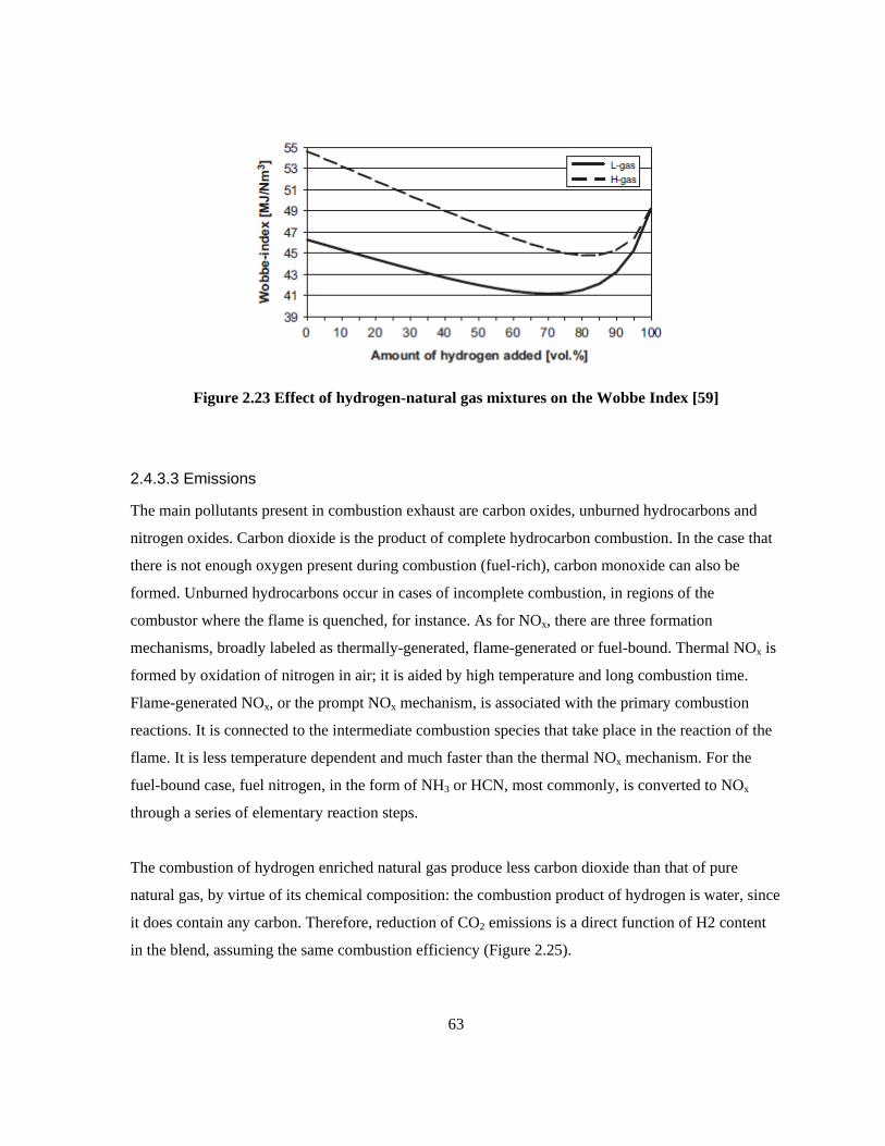
Figure 2.23 Effect of hydrogen-natural gas mixtures on the Wobbe Index [59]
2.4.3.3 Emissions
The main pollutants present in combustion exhaust are carbon oxides, unburned hydrocarbons and
nitrogen oxides. Carbon dioxide is the product of complete hydrocarbon combustion. In the case that
there is not enough oxygen present during combustion (fuel-rich), carbon monoxide can also be
formed. Unburned hydrocarbons occur in cases of incomplete combustion, in regions of the
combustor where the flame is quenched, for instance. As for NOx, there are three formation
mechanisms, broadly labeled as thermally-generated, flame-generated or fuel-bound. Thermal NOx is
formed by oxidation of nitrogen in air; it is aided by high temperature and long combustion time.
Flame-generated NOx, or the prompt NOx mechanism, is associated with the primary combustion
reactions. It is connected to the intermediate combustion species that take place in the reaction of the
flame. It is less temperature dependent and much faster than the thermal NOx mechanism. For the
fuel-bound case, fuel nitrogen, in the form of NH3 or HCN, most commonly, is converted to NOx
through a series of elementary reaction steps.
The combustion of hydrogen enriched natural gas produce less carbon dioxide than that of pure
natural gas, by virtue of its chemical composition: the combustion product of hydrogen is water, since
it does contain any carbon. Therefore, reduction of CO2 emissions is a direct function of H2 content
in the blend, assuming the same combustion efficiency (Figure 2.25).
63

Figure 2.24 Effect of hydrogen concentration in a CH4-H2 mixture on carbon emissions,
relative to pure CH4 [60]
The stoichiometric air/fuel mass ratio required for the complete combustion of hydrogen in air is
about 34:1, much higher than that of natural gas (17.2:1). This means that an air/fuel mass ratio that is
rich to hydrogen combustion is lean for natural gas combustion. Therefore, lean mixtures are possible
when burning hydrogen blended with natural gas, encouraging complete combustion. The high flame
velocity and the small quenching distance of hydrogen – the hydrogen flame is quenched closer to the
combustor than other fuels, increasing the reach of the flame – also encourage complete combustion.
Consequently, the carbon monoxide and unburned hydrocarbon emissions are reduced.
Dry low-emission premix combustors are proposed by manufacturers for natural gas applications.
They can reduce NOx emissions from gas turbines by mixing air to fuel before the combustion, so that
the air-fuel ratio in the primary zone of the turbine is higher than the stoichiometric ratio. For natural
gas with lower heating values -- hydrogen-enriched natural gas or coal syngas used in IGCC plants,
for example -- premixing becomes a questionable practice, because, hydrogen can react when mixed
to air at typical gas turbine conditions (wider flammability limits). Therefore, for fuels with hydrogen
content larger than 10%, premixing is excluded due to the potential of flashback [61]. In addition to
the risk of flashbacks, when pure hydrogen is fired, the higher flame temperature produces more
thermal NOx than the combustion of natural gas, if left untreated.
64

In these cases, fuel dilution by steam or nitrogen is required to bring emission levels within power
industry standards (22-45 ppmvd) by reducing flame temperature. In the case that a combined cycle is
present, steam is chosen as the diluent and extracted from the steam turbine. The combustion of pure
hydrogen, combined with the addition of diluent can impact the operation of a gas turbine in three
ways: the enthalpy drop during turbine expansion will vary, the flow rate of gas at the turbine inlet
will be different, and the heat-transfer coefficient, affecting the cooling of the turbine blades, will
differ.
2.4.4 Hydrogen Recovery and Use
The second of three pathways proposed for energy recovery is to use hydrogen by itself (Power to
Hydrogen), in specific downstream applications such as powering fuel cell vehicles, forklifts and
other vehicle prototypes, supplying needs of the manufacturing, food industries, and meeting
industrial and academic research uses. According to the Commodity Specification for Hydrogen
issued by the Compressed Gas Association, hydrogen used for general industrial applications (Grade
B) need to meet 99.95% overall hydrogen purity, and hydrogen for fuel, hydrogenation and water
chemistry applications (Grade D), 99.99%.
In the case that hydrogen is not produced "just-in-time", at the moment of its delivery, gas separation
technologies are required to produce hydrogen that meets end-user specifications, from the hydrogen-
natural gas mixture stored underground. Due to constraints in other energy recovery pathways
(material compatibility and fuel flexibility), the concentration of hydrogen in the mixture stream is
expected to be controlled to remain under 10%.
The driving force for all gas separation methods is the difference between one or more
physical/chemical properties of the components in a mixture. The properties behind the operating
principle of the most common gas separation technologies have been listed in Table 2.6. A given
method can only succeed, achieving the degree of separation wanted, if the components to be
separated differ in properties significantly.
Table 2.6 Separation methods and their corresponding properties [62]
65
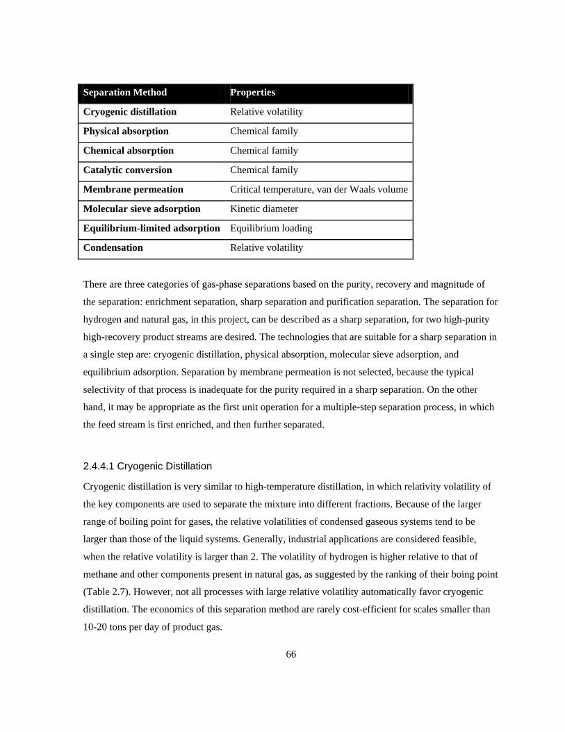
Separation Method Properties
Cryogenic distillation Relative volatility
Physical absorption Chemical family
Chemical absorption Chemical family
Catalytic conversion Chemical family
Membrane permeation Critical temperature, van der Waals volume
Molecular sieve adsorption Kinetic diameter
Equilibrium-limited adsorption Equilibrium loading
Condensation Relative volatility
There are three categories of gas-phase separations based on the purity, recovery and magnitude of
the separation: enrichment separation, sharp separation and purification separation. The separation for
hydrogen and natural gas, in this project, can be described as a sharp separation, for two high-purity
high-recovery product streams are desired. The technologies that are suitable for a sharp separation in
a single step are: cryogenic distillation, physical absorption, molecular sieve adsorption, and
equilibrium adsorption. Separation by membrane permeation is not selected, because the typical
selectivity of that process is inadequate for the purity required in a sharp separation. On the other
hand, it may be appropriate as the first unit operation for a multiple-step separation process, in which
the feed stream is first enriched, and then further separated.
2.4.4.1 Cryogenic Distillation
Cryogenic distillation is very similar to high-temperature distillation, in which relativity volatility of
the key components are used to separate the mixture into different fractions. Because of the larger
range of boiling point for gases, the relative volatilities of condensed gaseous systems tend to be
larger than those of the liquid systems. Generally, industrial applications are considered feasible,
when the relative volatility is larger than 2. The volatility of hydrogen is higher relative to that of
methane and other components present in natural gas, as suggested by the ranking of their boing point
(Table 2.7). However, not all processes with large relative volatility automatically favor cryogenic
distillation. The economics of this separation method are rarely cost-efficient for scales smaller than
10-20 tons per day of product gas.
66

Table 2.7 Boiling points of gas mixture components
Compound K
Butane 272
Propane 231
Carbon Dioxide 216
Ethane 184
Methane 109
Nitrogen 77.2
Hydrogen 20.1
In this approach, the components with higher condensation temperature (same as boiling temperature)
are condensed by Joule-Thompson refrigeration, derived from throttling the condensed liquid
hydrocarbons. Cryogenic distillation works best when the feed pressure is low, hydrogen
concentration in the feed is lower than 40%, and the heavier hydrocarbons are present in higher
concentrations and easily condensed. Hydrogen purity, recovery and pressure of the natural gas
stream are correlated, so not all of them can be optimized at the same time. If the natural gas stream,
produced after separation of hydrogen, has low pressure (0.7 bar), purities achievable is moderate
(90-95%) and the recovery of hydrogen is relatively high (90-95%) [63].
2.4.4.2 Physical Absorption
In absorption processes, the solute molecules are assimilated into a solid or liquid substance. Physical
and chemical absorption differ in the nature of the interaction between the absorbent material and the
solute molecules. The driving force in selective physical absorption is the difference in solubility.
Different gaseous solutes experience solubility in the absorptive liquid, due to different
intermolecular forces at play. Because of the use of a liquid absorbent, the physical absorption
process is sometimes called gas-liquid contacting.
The gas-liquid contacting process can be set up with a mixer and a separator unit. In this process, a
high pressure hydrogen-natural-gas stream is contacted with a liquid in a high pressure mixer unit, in
which the components of natural gas are selectively absorbed in the liquid. Solvents proposed for the 67

absorption of light hydrocarbons include iso-octane, n-octane, 1-octane or methyl cyclohexane. Then,
the gas and liquid phases are separated in a high pressure separator to obtain purified hydrogen
(Hydrogen has remained in the gas phase). The liquid containing dissolved natural gas is flashed at a
low pressure for regeneration, then returned to the mixer. The desorbed gas will still contain some
hydrogen, albeit at a lower concentration. Countercurrent version of this process has been proposed to
provide higher purity (85-95%) and recovery (85-95%) [63].
2.4.4.3 Adsorption
A molecular sieve is a material with holes small and precise enough to block large molecules,
allowing smaller molecules to pass. They select for adsorbent based on its molecular structure and
size. On the other hand, in equilibrium-limited adsorption, the extent of adsorption is determined by
the equilibrium loading of the adsorbent, typically expressed as isotherms. The most prevalent
adsorption process to separate hydrogen from other gases is the Pressure Swing Adsorption (PSA)
technology. In PSA, both driving forces for molecular adsorption and equilibrium-limited adsorption
may be in place, since molecular sieve is often used as adsorbent, and the force of adsorption is
dependent on the equilibrium loading of the adsorbent.
In this technology, the adsorbent attract other gases more strongly than it does hydrogen. So that
hydrogen is left free, while the rest is adsorbed. The adsorption takes place at a high pressure (10-40
bar) until the equilibrium loading is reached. At that point, no more adsorption capacity is available.
Once hydrogen has been removed from the chamber, partial pressure is lowered and the non-
hydrogen gases are desorbed, and the adsorbent, regenerated. After that, pressure is increased back to
adsorption level and the process resumes.
Separation through PSA is completed in batches, cyclically. Therefore, there is usually more than one
adsorption bed, so the overall process can be operated continuously: one unit desorbs while the other
begins absorption. Up to 12 units can be operated in concert. Hydrogen can be recovered at almost the
same pressure as feed pressure, since there is little pressure drop through the unit. Hydrogen purity
achievable is very high (99.99%), and moderate hydrogen recovery is possible (65-90%), depending
on the final pressure of the natural gas stream [63]. PSA systems are insensitive to changing feed
composition and provide constant product purity and recovery, once the exit gas stream pressure is
68

set. As the only separation technology that is able to meet the high purity requirement for fuel-grade
hydrogen, PSA is selected and modeled in this simulation study.
Different compounds have different potential for physical adsorption, conditional to operating
pressure, temperature and the component concentration inside the mixture. For PSA processes, inside
adsorption beds, the total system pressure is varied to control the adsorption equilibrium between the
adsorbed molecules and the adsorbent. Using a cycle of carefully designed operational steps that take
adsorbent regeneration into account, it is possible to use a batch of adsorbent to repeatedly separate a
continuously-fed stream of mixture.
Figure 2.25 Two-column four-step Skarstorm cycle [64]
2.4.5 Distribution of Hydrogen Enriched Natural Gas
The last energy recovery pathway considered for this project is the direct delivery of stored mixture, a
blend of hydrogen with natural gas, to gas end-users, through the existing local distribution pipelines
(Power to Gas). Hydrogen enriched natural gas (HENG) is not entirely new; prior to wide adoption of
69

natural gas as the key gaseous fuel, numerous countries used manufactured gas (or town gas),
consisting of 10 to 50% hydrogen, for lighting, heating and cooking through most of the 19th century
and the first half of 20th century. The distribution of HENG using existing natural gas infrastructure is
suggested by several authors, as an interim measure prior to large-scale pipeline delivery of pure
hydrogen or an opportunity to reduce the carbon emissions associated with natural gas use [59, 65,
66]. A project of special relevance is NaturalHy, a research project funded by the European
Commission’s Sixth Framework Programme, reuniting 39 partners to investigate the impact that the
additional to natural gas may have on the existing system.
Pipelines, compression stations and pressure-reduction stations form the existing natural gas
transportation infrastructure. The pressure drop in the pipeline between different compression stations
drives the flow of natural gas. The relationship between pipeline flow rate and the pressure drop is:
𝑄 = 𝐶𝐷2.5𝑒�𝑝12 − 𝑝22
𝑑𝑍𝑇𝐿𝑓
Where Q is the normal flow rate, Nm3/h; C is a dimensionless proportionality constant = 0.000129; D
is the pipeline inner diameter, mm; e the dimensionless pipeline efficiency, p1 and p2 are inlet and
outlet pressures, kPa; d the relative density compared to air; Z the compressibility factor; T the gas
temperature, K; L the pipeline length, K; f the dimensionless friction factor.
Because hydrogen has lower volumetric heating value compared to natural gas (Table 2.5), if pure
hydrogen is transported in the pipelines instead of natural gas, in order to maintain the same energy
flow, the volumetric flow of hydrogen Q needs to be three times that of natural gas. This increase in
Q is balanced by the decrease in density: hydrogen is approximately 9 times lighter than natural gas
(specific gravity of H2: 0.0696, specific gravity of natural gas: 0.6-0.7), so that the pressure drop
across the same section of pipeline can be maintained constant, despite of the change in gas
transported. Factoring changes in compressibility factor and friction factor, for the same pipeline and
pressure difference, pure hydrogen can transport 98% of the energy carried by lean natural gas under
the same conditions, and 80% of the energy carried by rich natural gas. For mixture of hydrogen with
natural gas at different concentration, the relative energy content is shown in Figure 2.27. It can be
observed that, for hydrogen concentration smaller than 20%, the energy flow carried by the mixture is
within 5% of that of pure natural gas.
70
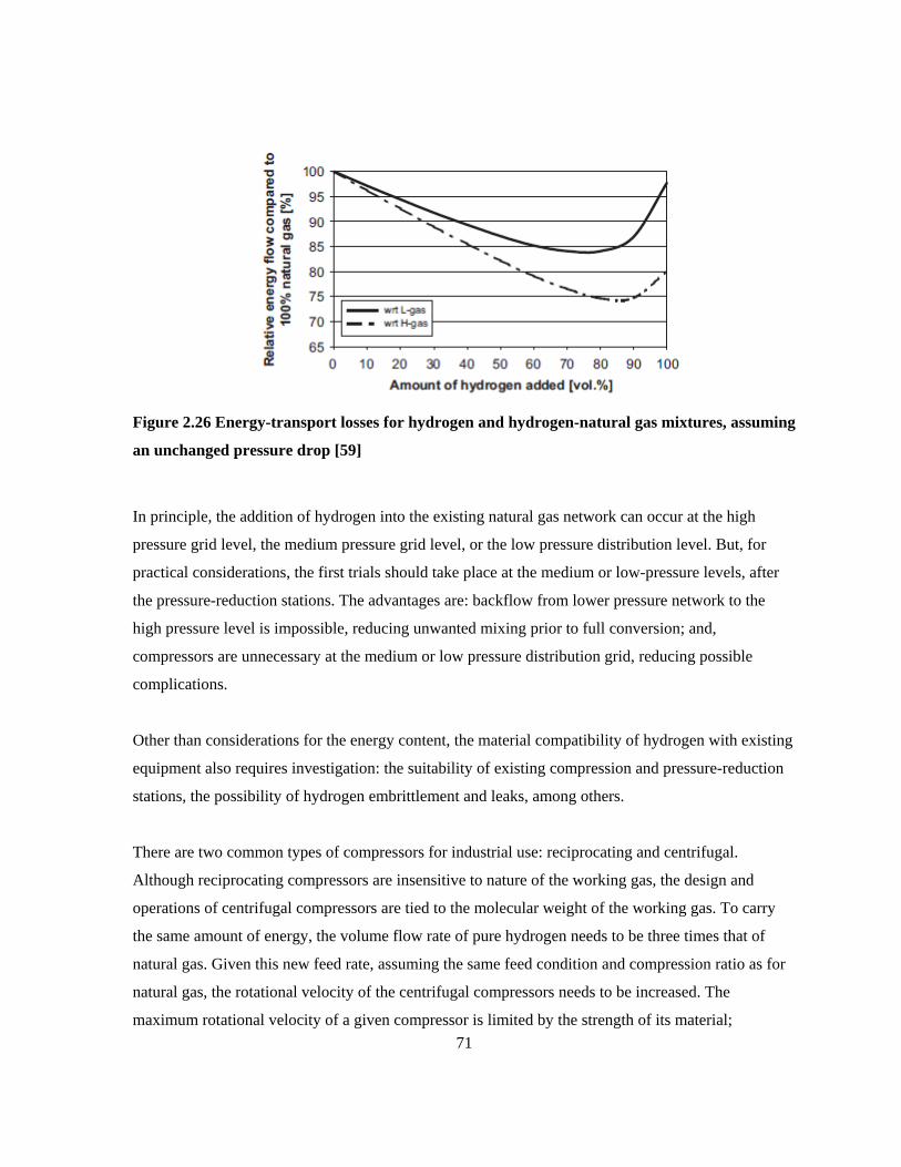
Figure 2.26 Energy-transport losses for hydrogen and hydrogen-natural gas mixtures, assuming
an unchanged pressure drop [59]
In principle, the addition of hydrogen into the existing natural gas network can occur at the high
pressure grid level, the medium pressure grid level, or the low pressure distribution level. But, for
practical considerations, the first trials should take place at the medium or low-pressure levels, after
the pressure-reduction stations. The advantages are: backflow from lower pressure network to the
high pressure level is impossible, reducing unwanted mixing prior to full conversion; and,
compressors are unnecessary at the medium or low pressure distribution grid, reducing possible
complications.
Other than considerations for the energy content, the material compatibility of hydrogen with existing
equipment also requires investigation: the suitability of existing compression and pressure-reduction
stations, the possibility of hydrogen embrittlement and leaks, among others.
There are two common types of compressors for industrial use: reciprocating and centrifugal.
Although reciprocating compressors are insensitive to nature of the working gas, the design and
operations of centrifugal compressors are tied to the molecular weight of the working gas. To carry
the same amount of energy, the volume flow rate of pure hydrogen needs to be three times that of
natural gas. Given this new feed rate, assuming the same feed condition and compression ratio as for
natural gas, the rotational velocity of the centrifugal compressors needs to be increased. The
maximum rotational velocity of a given compressor is limited by the strength of its material; 71

therefore, the compression of pure hydrogen may be unsuitable with centrifugal compressors
currently in use.
Hydrogen embrittlement is the diffusion of hydrogen atoms through various metals (especially steel),
creating pressures within the metal that reduces their ductility and tensile strength, leading up to
hydrogen induced cracking. The risk of damage to pipelines is dependent on its material of
construction and its history: larger fluctuations experienced by the pipeline increase the risk of
hydrogen embrittlement and material fatigue. Results from fracture toughness tests and fatigue tests
performed in the NaturalHy project suggest that up to 50% hydrogen can be accommodated in
pipelines, without significant effect on embrittlement for the pipeline material tested. Other studies
have provided more conservative values, showing that up to 17 % of hydrogen can be accommodated.
Diffusion losses of gas occur through seals, gaskets, valves and fittings. The diffusion loss of
hydrogen will be larger than natural gas, for the same equipment designed to contain natural gas. The
hydrogen molecule has a smaller size and lower viscosity. Since the 1980’s, polyethylene pipelines
have been used by many gas distributors at the low pressure distribution network level. Diffusion of
hydrogen loss through such pipelines is five times more important than that of natural gas. Overall,
the diffusion losses are considered negligible, at approximately 0.0005-0.001% of the totally
transported volume [59].
72

Chapter 3 Model Overview
Prior to the formal development of the physical and the performance models, as indicated by the
research objectives, the key decision variables, equivalent to user-manipulated inputs, and the
performance indicators, equivalent to model outputs from simulation, need to be outlined. The inputs
and outputs are of key interest, since they determine the level of detail of model development. In this
chapter, after a detailed view of the energy hub, the key decision variable and performance indicators
identified are described.
3.1 Energy Hub Overview
The energy hub, first sketched in Figure 1.4, can be further broken down to show its internal
components and interconnections in Figure 3.1. Within the confine of the dashed line, which
represents the physical boundary of the energy hub, the main technological components are labelled:
the wind turbines, the electrolyzers, the storage reservoir, the CCGT plant and the PSA separator. The
compressor units needed are numbered from C1 to C4; they are identical blocks, only the feeds are at
different conditions. Additionally, because this modeling study is not intended for optimization,
additional specifications that define the relationship between two or more variables are required, so
that the model can become fully specified. The colored diamonds (D1 through D6) represent such
decision points.
73

Figure 3.1 Detailed view of the energy hub
74

3.2 Decision Variables
The decision variables are also known as experimental factors or model inputs; they are elements of
the model which can be altered to effect better understanding of the real world system. They are also
known as experimental factors. Three types of decision variables have been identified for the
simulation of the energy hub:
1. Variables that describe the configuration of energy hub components (Ex: with or without
separator, with or without CCGT);
2. Variables that describe the rated capacity of energy hub components (Ex.: the rated
input/output of the electrolyzer, the rated input/output of the separator);
3. Relationships that can determine the value of unspecified variables based on specified ones.
Type 1 and 2 variables have been identified and listed in Table 3.1. Note that the storage reservoir is
always set to be available; otherwise, the energy hub project wouldn’t be physically meaningful.
Also, its storage capacity and rated input/output (known as injectability/deliverability for reservoirs)
are taken to be fixed, for they cannot be freely adjusted as for individual man-made parts.
Table 3.1 List of system configuration and capacity variables
Component Variable Symbol Value Unit Reference
Reservoir (ON) Rated capacity max,sV 7.6 Bcf [67]
Electrolyzers (ON/OFF)
Rated capacity per unit , ,E rated iP 0.29 MW [68]
Number of units EN integer ≥ 0
Wind turbines (ON/OFF)
Rated capacity per unit , ,W rated iP 2 MW [69]
Number of units TN integer ≥ 0
CCGT (ON/OFF) Rated capacity ,CC ratedW 40-800 MW [58]
Separator (ON/OFF)
Rated capacity ,feed ratedV 300-400,000 Nm3/h [70]
75

The last type of decision variables/relationships is necessary because this modeling project is not
based on optimization, which can be set up to determine the optimal values of unspecified variables
automatically. For the model simulation to arrive at results, the system of equations that is the model
needs to be completely specified.
Each of the six decision points, shown in Figure 3.1, represents the logic for one or more of the
relationships required. The pairs of variables that they connect are shown in Table 3.2.
1. At decision points 1, it is necessary to determine whether to inject into the reservoir, produce
from the reservoir, or shut-in the reservoir based on exogenous power and gas market
conditions. The reservoir model then translates the “mode”, also referred to as the reservoir
dispatch order, into injectability or deliverability terms;
2. At decision point 2, it is necessary to determine the utilization level of the electrolyzer and
the mix of power supply used;
3. At decision point 3, it is necessary to determine whether the electrolytic hydrogen produced
is sent to storage, or directly delivered to meet local demand for hydrogen;
4. At decision point 4, it is necessary to determine how much natural gas to blend with the
hydrogen produced;
5. At decision point 5, it is necessary to determine the amount of mixture is withdrawn from
storage, and the amount dispatched to different energy recovery pathways;
6. Finally, at decision point 6, the destination of the natural gas-rich stream from the separator
needs to be decided. For simplicity, it is assumed that it is merged with the mixture
dispatched to the gas distribution network.
Compared to the first two types of decision variables, for which binary values (ON/OFF) or a simple
number suffice, the decision points require inputs which are more complex. In Chapter 7, when
describing inputs for different scenarios, the decision points are illustrated by logic flow diagrams.
76

Table 3.2 List of decision point inputs and outputs
Description Inputs Symbol Unit Outputs Symbol
Unit
D1 Reservoir operation regime
Sets of exogenous environmental variables and their derivatives
Reservoir mode
Mode N/A
H2 produced 2 ,H En kmol/h
D2 Electrolyzer power supply
Sets of exogenous environmental variables and their derivatives
Wind power stored
WtsP MW
Wind power available WP MW Wind power
sold to grid WtGP MW
Rated power of electrolyzers
,E ratedP MW Grid power stored
GtsP MW
Electrolyzers supply
EP MW
D3 Hydrogen bypass
H2 produced 2 ,H En kmol/h H2 stored
2 ,H sn kmol/h
Injectability/deliverability
sn kmol/h H2 bypassed 2 ,H bn kmol/h
H2 demand schedule 2 ,H loadn kmol/h H2 curtailed
2 ,H cn kmol/h
D4 NG/H2 blending
H2 stored 2 ,H sn kmol/h NG stored
,NG inn kmol/h
Injectability/deliverability
sn kmol/h Mixture stored
,mix inn kmol/h
H2 conc. 2 ,H inc mol %
D5 Mixture dispatch
Injectability or deliverability
sn kmol/h Fuel to CCGT
fueln kmol/h
Rated fuel capacity of CCGT
,fuel ratedn
kmol/h Feed to separator
feedn kmol/h
Rated feed capacity of separator
,feed ratedn
kmol/h Mixture delivered
mixn kmol/h
Mixture withdrawn
,mix outn
kmol/h
D6 Separator recycle
Waste stream from separator
,sep mixn kmol/h Mixture delivered
,mix totn
kmol/h
Curtailed separator feed
,feed cn kmol/h H2 conc. in mixture delivered
2 , ,H mix toc
mol %
Mixture delivered mixn kmol/h
H2 concentration in waste 2 , ,H sep mixc
mol %
Reservoir H2 conc. 2 ,H resc mol %
77

3.3 Exogenous Variables
The exogenous variables are variables describing elements which are outside of the scope of this
modeling study. They are presented here, because they are the basis of many operational decisions at
decision points. In the following sections, each of the external components that interact with the
energy hub is discussed in terms of the direction for material flow, the realistic scale of supply and/or
demand, and the information available to energy hub operators for decision making.
The exogenous environmental variables are dependent on the geographic location and the temporal
coverage of the energy hub project. For this simulation study, they are taken to be constants, but they
can be updated with different values to assess the same energy hub project planned for other locations
and/or time periods.
In this study, it is assumed that they interact with the energy hub but are not changed by outputs from
the energy hub. For example, it is assumed that the market price of electricity is not influenced by the
electricity consumed or supplied by the energy hub. Such assumptions may be valid for energy hubs
with relatively limited inputs and outputs; once their scale and number multiply, it will be necessary
to re-evaluate such assumptions.
Also, in this modeling project, external components are usually represented by their aggregated
behaviour – for example: the overall Ontario demand for electricity –, but, in reality, each of them is
made up of many smaller constituents, for example: the power grid is made up of many other power
suppliers and loads. If the previous assumption is found to be invalid, then such aggregated
representation of the external components will need to be revised; the inner details of the power grid
and the natural gas grid will need to be modeled, thus transforming them from exogenous variables
endogenous variables of the modeling efforts.
78

Table 3.3 List of exogenous environmental variables
Component Variable Symbol Value Unit Reference
Power grid Market price of electricity
HOEP Figure 3.4 Historic HOEP from 2010-2012
$/MWh [14]
Ontario demand loadP Figure 3.5 Historic Ontario electricity demand for 2010-2012
MW [14]
FIT price schedule
FIT Weekdays 11am-6pm: 135% of 115
Rest of the week: 90% of 115
$/MWh [71]
Emission factor of power from grid
GEF Figure 3.8 Hourly emission factor for power generation in Ontario for 2010-2012
kg CO2
/MWh [106]
Natural gas grid
Market price of natural gas
NGC Figure 3.11 Historic natural gas spot price at Henry Hub for 2010-2012
$/MMBtu [72]
Mixture demand
Price of mixture
mixC Identical to natural gas market prices
$/MMBtu Estimated in section 3.3.3
Hydrogen demand
Price of hydrogen
2HC 5 $/kg Estimated section 3.3.4
Hydrogen pick-up schedule
2 ,H loadn Weekdays 10am – 5pm: >0
Rest of the week: 0
kmol/h Assumed
79

3.3.1 Power Grid
The power grid is both a source and a sink for electricity. The energy hub, since it has the capability
to generate and consume electricity, has a bidirectional relationship with the power grid (Figure 3.2).
But, for any given hours, it is assumed that the energy is either producing or consuming electricity,
not both simultaneously.
Figure 3.2 Interaction between the power grid and energy hub
In reality, the Ontario power grid is an extended network made up of 30,000 km of high-voltage
transmission lines, spanning all regions of Ontario, connecting power generators with loads. It would
be necessary to capture the geographic disaggregated nature of the power grid, if it were modeled as
an endogenous component of the project, including the location of different generators and loads, the
status of connections between them (congested or not), and the status of generators and loads (Figure
3.3). However, given that the power grid is considered to be exogenous to the scope of the current
project, it is modeled as a single connection to the energy hub, through which electricity can be
procured and delivered.
The power grid interacting with the energy hub can be viewed as a provincial system. For the
volumes of imports and exports are small compared to the overall volumes of intra-province
production and consumption. For the year of 2011, imported electricity fulfilled 3% of the total
Ontario demand, whereas 9% of electricity produced in Ontario was exported (calculated from IESO
market data). Given the scale of the Ontario power grid (34,000 MW installed by end of 2011 and
150.4 TWh generated for the year of 2011), it is assumed that the planned energy hub (1 to 50 MW in
scale) will not have significant influence over the grid-wide power supply and demand. 80

Figure 3.3 Ontario's power grid and its transmission zones [73]
The wholesale market price of electricity (HOEP) is the main tool through which the operations of
many different electricity market participants are coordinated. The historic HOEP for 2010 through
2012 is published as part of the market data archive by the IESO (Figure 3.4).
Other than the market price, the IESO also publishes the actual level of demand in Ontario at an
hourly resolution (Figure 3.5). Upon inspection, it is found that the market price shows some
correlation with the power demand (correlation coefficient r = 0.44, suggesting modest correlation).
Also, comparing the two measures by plotting the relative change with respect to the previous value
in the time series, it is observed that the market price for electricity is much more volatile than the
demand for electricity (Figure 3.7). Therefore, in some scenarios, the HOEP is interpreted as an
indicator of the level of demand and supply within the electricity market, guiding the operations of
the energy hub as it is the only information realistically available in real-time. But, in some other
scenarios which have particular focus on better serving the electricity demand in Ontario, the actual
81

market demand data is used as the indicator, for it is a more accurate measure for hourly demand in
Ontario.
Figure 3.4 Historic HOEP from 2010-2012
Q3 2010
-1000100200300400500
82

Figure 3.5 Historic Ontario electricity demand for 2010-2012
Figure 3.6 Correlation between 2010-2012 electricity demand and HOEP for Ontario
Q3 2010
0K5K10K15K20K25K
83

Because of the existence of the Feed-In Tariff (FIT) program in Ontario, a participating renewable
energy generator is paid a price different than the HOEP. The FIT price is fixed and reviewed
annually; for current wind projects, it is $115/MWh [71]. For technologies which are dispatchable,
the FIT schedule is multiplied to a factor to incentivise production during peak periods. The rate paid
during peak periods (weekdays from 11am to 6pm, inclusively) is 135% of the fixed FIT price, and
the rate paid ruing off-peak periods (rest of the time, including weekends) is 90% of the fixed FIT
price. In this project, it is assumed that wind power generated on-site, given that it can be directed to
storage, is considered to be dispatchable, being paid the time-differentiating FIT schedule instead of
the fixed price.
Figure 3.7 Relative hourly changes in HOEP and Ontario demand
84

Finally, in order to assess the carbon dioxide emissions incurred when the energy hub consumes
electricity purchased from the grid, it is necessary to have access to the emission factor of grid power
in Ontario. Currently, an annual greenhouse gas intensity factor is available for Ontario’s electricity
system in general, but it does not reflect the hourly variation in emission caused by the different types
of generators engaged. For this project, the hourly emission factor for electricity generation in Ontario
is estimated from the hourly total generation, the hourly wind power generated, percentage of energy
by fuel type (annual values), and an approximate merit order (Figure 3.8).
Figure 3.8 Hourly emission factors for power generation in Ontario for 2010-2012
85

3.3.2 Natural Gas Grid
The natural gas that is stored in the underground reservoir, along with hydrogen, is supplied by the
high pressure transmission pipelines of the natural gas grid (Figure 3.9). The mixture withdrawn from
storage is not sent back to the original natural gas grid: it is assumed that the gas exiting the energy
hub, in the form of a natural gas/hydrogen mixture, is distributed directly to local consumers via a
series of dedicated mid-to-low pressure distribution pipelines. These dedicated pipelines might be
assets formerly belonging to the natural gas grid, but they are differentiated from the natural gas grid
in general because of their dedicated content (discussed in Section 3.3.3).
Figure 3.9 Interaction of the natural gas grid with the energy hub
Ontario is the largest market for natural gas in Canada, with a peak demand of 3 Bcf per day.
Compared to the total annual consumption of 756.5 Bcf, the annual marketed production in Ontario is
only 8.32 Bcf [74]. Therefore, Ontario is largely dependent on external producers, mostly form the
Western Canada Sedimentary Basin, for its own natural gas needs. The province receives natural gas
from producers in western Canada through the northern mainline TransCanada Pipeline (TCPL, 4.1
Bcf per day), and through Dawn Hub in southwestern Ontario (3.9 Bcf per day) [75]. The major
natural gas pipelines entering and leaving Ontario are shown in Figure 3.10. Pipeline capacity in
excess of Ontario’s needs, approximately 60 percent of the gas entering Ontario, is used to supply
Eastern Canada and the North Eastern US markets. Compared to the Ontario power market, which is
essentially provincial, the natural gas market of Ontario is tightly coupled to the supply and demand
in other jurisdictions.
86
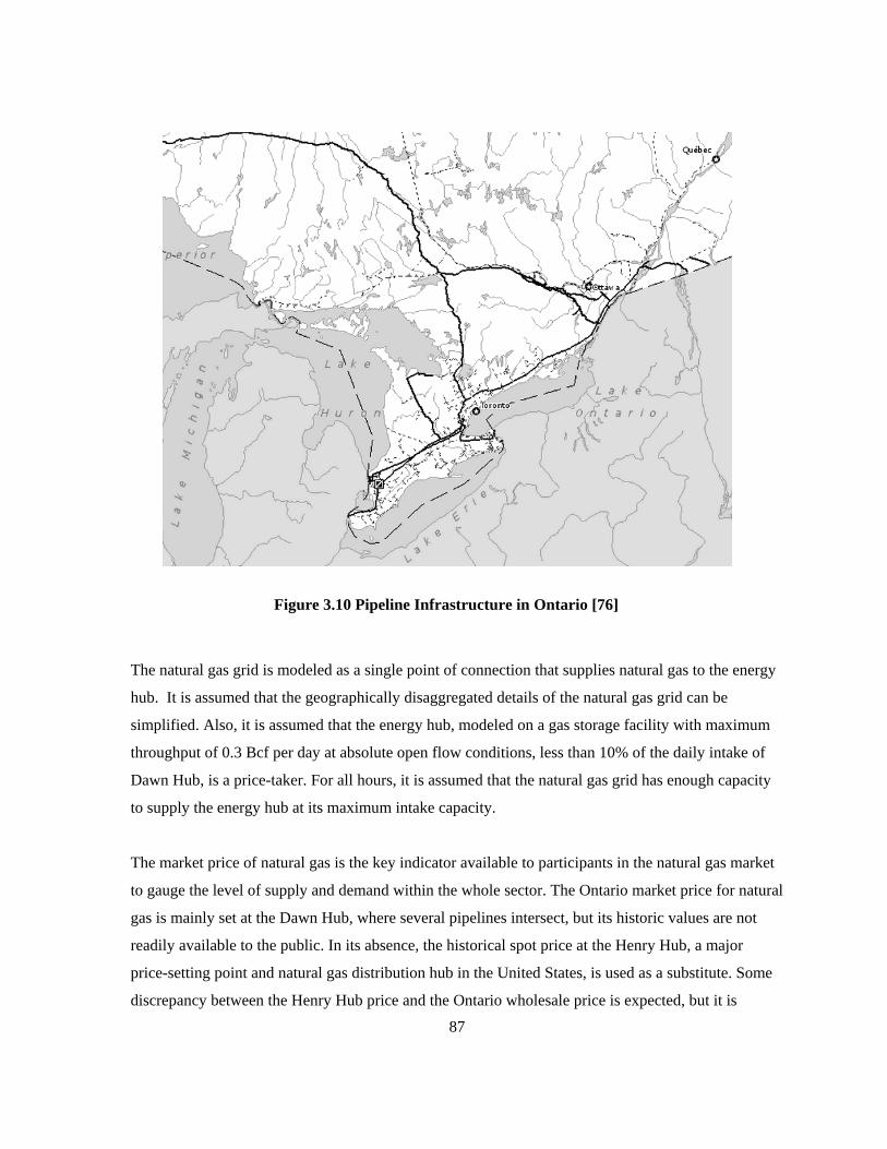
Figure 3.10 Pipeline Infrastructure in Ontario [76]
The natural gas grid is modeled as a single point of connection that supplies natural gas to the energy
hub. It is assumed that the geographically disaggregated details of the natural gas grid can be
simplified. Also, it is assumed that the energy hub, modeled on a gas storage facility with maximum
throughput of 0.3 Bcf per day at absolute open flow conditions, less than 10% of the daily intake of
Dawn Hub, is a price-taker. For all hours, it is assumed that the natural gas grid has enough capacity
to supply the energy hub at its maximum intake capacity.
The market price of natural gas is the key indicator available to participants in the natural gas market
to gauge the level of supply and demand within the whole sector. The Ontario market price for natural
gas is mainly set at the Dawn Hub, where several pipelines intersect, but its historic values are not
readily available to the public. In its absence, the historical spot price at the Henry Hub, a major
price-setting point and natural gas distribution hub in the United States, is used as a substitute. Some
discrepancy between the Henry Hub price and the Ontario wholesale price is expected, but it is
87

assumed to be negligible; the natural gas price in Canada is linked to the American natural gas market,
for natural gas is imported and exported extensively across international borders and the prices are
competitively set.
Unlike electricity, whose market price is set every hour (or at even shorter intervals), the historic
price of natural gas is only available at a daily resolution (weekdays only, excluding week days and
holidays, [72]). Consequently, in order to generate an hourly time series for the simulation, weekly
averages of the Henry Spot price are computed and expanded to hourly resolution (i.e. all hours in the
same week has the same natural gas price).
Figure 3.11 Historic natural gas spot price at Henry Hub for 2010-2012
Q1 2010
0123456
88

3.3.3 Mixture Demand
The mixture demand is the sink for which all mixture produced from the energy hub for off-site use.
In this project, it is assumed that the demand for hydrogen-enriched natural gas is fulfilled via the use
of existing natural gas distribution network, but, in order to assess the scale of demand, it is treated
separately from the natural gas demand in general.
Figure 3.12 Interaction of the mixture need with energy hub
In the near future, hydrogen enriched natural gas is expected to be used as an alternative to
conventional natural gas; therefore, the projection of demand for such mixture is based on the current
demand for natural gas in Southwestern Ontario, the region in which the energy hub is to be located.
The Ontario total natural gas consumption for year 2010-2012 is shown in Figure 3.13. Assuming
natural gas use is proportional to population, then the annual natural gas consumption of
Southwestern Ontario is estimated to be 27% of the total Ontario demand. Then, it is assumed that
10% of the Southwestern Ontario demand can be converted to use hydrogen-enriched natural gas as a
substitute. The resulting estimate for mixture demand for the period of interest is shown by the line in
the same figure.
Since the hydrogen/natural gas mixture a new product without an established market price, a selling
price needs to be established, considering the possible end-users and competitors. The price that
newly converted industrial customers are willing to pay is likely to be the price that they are currently
paying for natural gas. Therefore, the selling price of the mixture is set to be identical to the price of
natural gas; note that the price is expressed in terms of energy content, not mass or volume.
89

Figure 3.13 Ontario monthly natural gas demand for 2010 – 2012 [77]
Q2 2010
0K20K40K60K80K100K120K
0K
Measure Names
90

3.3.4 Hydrogen Demand
The hydrogen demand is the sink for all pure hydrogen delivered from the energy hub (Figure 3.14).
Compared to other sinks (the power grid and the demand for mixture), the demand for hydrogen is
different in that is does not yet have dedicated transport infrastructure, such as power lines or gas
distribution pipelines, so that the demand is not always present: hydrogen demand is present only
when there is a scheduled delivery to be made. Therefore, during simulation, the effect of constrained
delivery needs to be investigated.
Figure 3.14 Interaction of Hydrogen Need with Energy Hub
Proponents of the hydrogen economy propose that, as part of the efforts to decarbonize modern
society’s energy use, hydrogen can be and should be used as an energy vector. But, at the present
stage, hydrogen is still mainly used as an industrial commodity, a feedstock to be used in other
industrial processes. The main industrial usages of hydrogen include heavy oil upgrading, oil refining,
ammonia and methanol production. These constitute 85% of hydrogen consumption in Canada. The
other 15% of consumption, outside of process need, include the heat treatment of metals, glass
making, microelectronics fabrication, power generator cooling, hydrogenation of food oils, as well as
the nascent fuel cell applications [78].
In 2008, 3 megatonnes of hydrogen was produced in Canada, of which 70% was produced from
natural gas, via steam methane reforming [79]. Using the information above, it is calculated that the
per capita hydrogen consumption in Canada is about 87 kg per year. The region of interest to this
simulation project, Southwestern Ontario, centered on the city of London, containing Lambton
County, in which the storage reservoir is to be located, has a population of 3,443,484 in 2006.
Therefore, a first estimate for the regional consumption of hydrogen would be about 300,000 tonnes
91

annually. For the scale of electrolyzer operations envisaged (1MW to 20 MW), supposing 100%
utilization and 70% efficiency converting power to hydrogen, a maximum annual production in the
order of 3000 tonnes is possible, or 1% of the projected regional demand. Therefore, it seems
reasonable to assume that the existing demand for hydrogen can absorb the hydrogen produced at the
energy hub.
Unlike for natural gas and electricity, there is no publicly disclosed market price for hydrogen.
Therefore, the price at which hydrogen is delivered to consumers is estimated according to the
following guidelines:
In accounting, two long-run pricing approaches are common: the market-based approach and the cost-
based approach [80]. Because hydrogen is a commodity product, as opposed to differentiated
products such as cameras and cars, the market-based approach is recommended, for competition
between producers is an important market force in this case. The market-based pricing approach
requires knowledge of the price that potential customers are willing to pay. This price can be
estimated based on the understanding of the value that customers perceive in the product, and on the
knowledge of the price of competing products.
Of all the applications for electrolytic hydrogen, using it as an alternative fuel to replace gasoline or
using it in conventional industrial and research applications to replace hydrogen produced via SMR
are perceived as the most important.
Assuming that the main value that the customers perceive in the energy-hub produced hydrogen is its
value as an alternative fuel, the price that the customers are willing to pay for hydrogen will be the
expected price of retail gasoline, perhaps at a premium, given that hydrogen is a cleaner-burning fuel.
The historic retail price of gasoline is, obtained from the Energy Information Administration, shown
in Figure 3.15 suggests that for the future five years, the per-gallon price of gasoline will vary in
between $2 and $4. Given that 0.997 kg of hydrogen constitutes 1 gasoline gallon equivalent, the
price that the customers are willing to pay should also vary from $2 to $4.
Assuming that the main value that the customers perceive in the energy-hub produced hydrogen is its
ability to replace hydrogen produced from natural gas, then the cost of such fossil-fuel based
hydrogen needs to be examined. As shown by Figure 3.11, natural gas prices in recent years vary
between $2/MMBtu to $5/MMBtu (~ $2 to $5/GJ). Thus, using the correlation given by Figure 3.16,
92

the cost of hydrogen should range from $10 to $25/GJ ($1.2 to $3/kg hydrogen), for centralized SMR
and distributed SMR respectively.
Figure 3.15 Historic retail price of regular gasoline from 1991 to 2012
1994
01234
Average
93
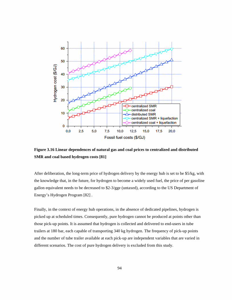
Figure 3.16 Linear dependences of natural gas and coal prices to centralized and distributed
SMR and coal based hydrogen costs [81]
After deliberation, the long-term price of hydrogen delivery by the energy hub is set to be $5/kg, with
the knowledge that, in the future, for hydrogen to become a widely used fuel, the price of per gasoline
gallon equivalent needs to be decreased to $2-3/gge (untaxed), according to the US Department of
Energy’s Hydrogen Program [82] .
Finally, in the context of energy hub operations, in the absence of dedicated pipelines, hydrogen is
picked up at scheduled times. Consequently, pure hydrogen cannot be produced at points other than
those pick-up points. It is assumed that hydrogen is collected and delivered to end-users in tube
trailers at 180 bar, each capable of transporting 340 kg hydrogen. The frequency of pick-up points
and the number of tube trailer available at each pick-up are independent variables that are varied in
different scenarios. The cost of pure hydrogen delivery is excluded from this study.
94

3.4 Performance indicators
Performance indicators are the results generated by the model based on the inputs provided. The
interpretation of those indicators is the source of much insights gained from a modeling and
simulation study. As discussed previously, there are three types of performance indicators: physical,
financial and environmental. The financial and environmental performance indicators are evaluated
using the physical indicators. The physical model outputs of interest are summarized by the Table 3.4.
All of the physical performance indicators are available as hourly time series for the time period
simulated. They can also be compared in their aggregate form. The outputs are separated into two
types: stock variables, for which the annual average of the time series is more meaningful, and flow
variables, for which the annual sum of the time series is more meaningful.
95

Table 3.4 List of physical performance indicators
Component Variable Symbol Description Type Unit
D1 Dispatch order to the reservoir
Mode The dispatch order indicates the decision of the operators to inject/withdraw gas from the reservoir
Stock N/A
Storage reservoir
Inventory totaln The total amount of gas in storage Stock kmol
H2 conc. 2 ,H resc Hydrogen concentration of the gas mixture in storage Stock mol %
Reservoir pressure resp Pressure that the gas in storage exerts on the reservoir, assumed to be uniform
throughout Stock bar
Wellhead pressure whp The pressure at the wellhead, which is controlled by the operators of the energy hub Stock bar
Injectability/deliverability sn The physical limits to flow rates in/out of the reservoir, given the conditions of the
reservoir Flow kmol/h
Actual flow rate ,s actn The actual flow rate of gas injected or withdrawn, maybe lower than or equal to the
injectability / deliverability Flow kmol/h
Wind turbines
Wind power produced WP Wind power generated by the on-site wind turbine Flow MW
Utilization factor WU The capacity utilization factor for the individual component Stock
D2 Wind power stored WtsP The amount of wind power produced that is supplied to the electrolyzers Flow MW
Wind power sold to grid WtGP The amount of wind power produced that is supplied to the power grid Flow MW
Grid power stored GtsP The amount of grid power that is supplied to the electrolyzers Flow MW
Electrolyzers H2 produced 2,H En Amount of hydrogen produced by the electrolyzers Flow kmol/h
Utilization factor EU The capacity utilization factor for the individual component Stock
D3 H2 stored 2 ,H sn The amount of hydrogen produced by the electrolyzers that is injected into the reservoir Flow kmol/h
H2 bypassed 2 ,H bn The amount of hydrogen that is delivered to meet demand upon production from the Flow kmol/h
96
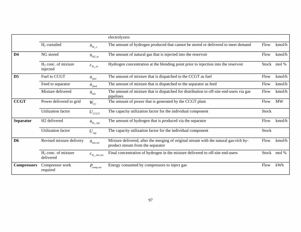
electrolyzers
H2 curtailed 2 ,H cn The amount of hydrogen produced that cannot be stored or delivered to meet demand Flow kmol/h
D4 NG stored ,NG inn The amount of natural gas that is injected into the reservoir Flow kmol/h
H2 conc. of mixture injected 2 ,H inc Hydrogen concentration at the blending point prior to injection into the reservoir Stock mol %
D5 Fuel to CCGT fueln The amount of mixture that is dispatched to the CCGT as fuel Flow kmol/h
Feed to separator feedn The amount of mixture that is dispatched to the separator as feed Flow kmol/h
Mixture delivered mixn The amount of mixture that is dispatched for distribution to off-site end-users via gas
pipelines Flow kmol/h
CCGT Power delivered to grid CCW The amount of power that is generated by the CCGT plant Flow MW
Utilization factor CCGTU The capacity utilization factor for the individual component Stock
Separator H2 delivered 2 ,H sepn The amount of hydrogen that is produced via the separator Flow kmol/h
Utilization factor sepU The capacity utilization factor for the individual component Stock
D6 Revised mixture delivery ,mix totn Mixture delivered, after the merging of original stream with the natural gas-rich by-
product stream from the separator Flow kmol/h
H2 conc. of mixture delivered 2 , ,H mix totc Final concentration of hydrogen in the mixture delivered to off-site end-users Stock mol %
Compressors Compressor work required
,comp totP Energy consumed by compressors to inject gas Flow kWh
97

As outlined in the conceptual model, the financial is one of the evaluative models that assess the
performance of the energy hub project. The key indicators developed and used is the: net present
value of project which captures the main economic benefits directly associated with the operations of
the energy hub. The constituents required for the calculation of the net present value are many. Each
of the shadowed boxes in Figure 3.17 can be further divided into its constituents; they are described
in Chapter 5. The default project life time used is 20 years; and the discount rate is 8% for final
reporting.
Figure 3.17 Scope for financial model
For this study, only carbon dioxide emissions are included as part of the emission model to facilitate
model development. The scope of emission model is drawn to include emissions incurred while
operating the energy hub and emissions that are displaced by the operations of the energy hub, so that
the net emissions associated with the energy hub can be assessed (Figure 3.18).
The sources of emissions associated with the energy hub are: emissions from power generators which
produce the electricity for hydrogen production, including both the grid-connected generators and the
on-site wind turbines; emissions from on-site use of hydrogen-enriched natural gas at the CCGT;
emissions from the off-site use of the hydrogen/natural gas mixture by the end-users reached by the
distribution pipeline, and emissions from the natural gas-driven compressors that enable gas injection.
98
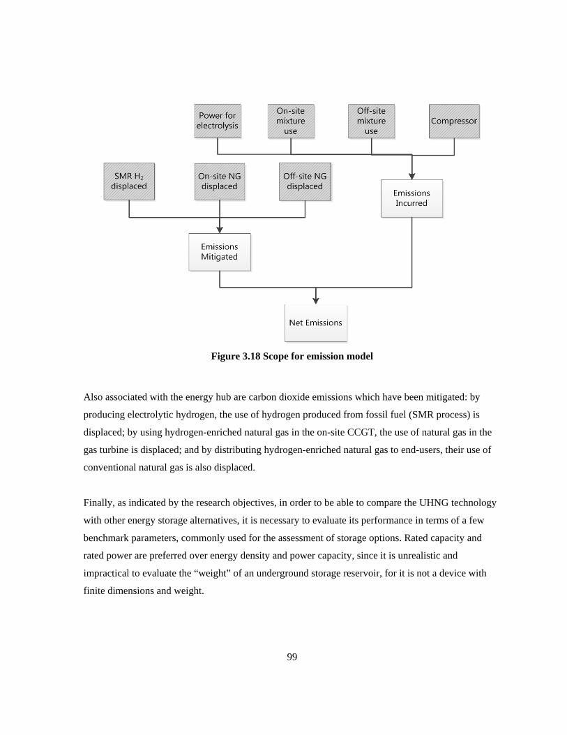
Figure 3.18 Scope for emission model
Also associated with the energy hub are carbon dioxide emissions which have been mitigated: by
producing electrolytic hydrogen, the use of hydrogen produced from fossil fuel (SMR process) is
displaced; by using hydrogen-enriched natural gas in the on-site CCGT, the use of natural gas in the
gas turbine is displaced; and by distributing hydrogen-enriched natural gas to end-users, their use of
conventional natural gas is also displaced.
Finally, as indicated by the research objectives, in order to be able to compare the UHNG technology
with other energy storage alternatives, it is necessary to evaluate its performance in terms of a few
benchmark parameters, commonly used for the assessment of storage options. Rated capacity and
rated power are preferred over energy density and power capacity, since it is unrealistic and
impractical to evaluate the “weight” of an underground storage reservoir, for it is not a device with
finite dimensions and weight.
99

Table 3.5 List of energy storage benchmark parameters
Parameter Description Unit
Round trip
efficiency
Defined as the AC to AC efficiency, involving all conversion steps in
between
Rated capacity The maximum amount of electrical energy that can be stored (usually
in the form of another vector)
MWh
Rated power The maximum rate at which electricity can be stored or discharged MW
Self-discharge
rate
The rate at which stored energy is lost from storage
Durability The physical life time of the project years
Cost of storage The capital cost required to setup storage facility, expressed both in
terms storage capacity ($/MWh) and rated power ($/MW)
$/MWh
$/MW
100

Chapter 4 Physical Model Development
The physical model is made up by smaller models, each representing a component of the energy hub:
the storage reservoir, wind turbines, electrolyzers, the gas turbine, the separator, and compressors.
The decision points connect individual component models and allow for interaction with the
exogenous environmental variables.
The architecture of the overall physical model is illustrated by Figure 4.2: Information flow from the
top to the bottom. Decision points are shown as diamonds and the component technologies sub-
models, are shown as double-sided boxes. Once simulation is initiated, information about the decision
variables: configuration of energy hub, ratings of components, and the model logic of all decision
points are loaded into the model. After initialization, the model logic at D1 and D2 drives the key
activities at the storage reservoir: dictating the operations occurring at the storage reservoir and the
electrolyzer, respectively. Their outputs are in turn routed toward D3, D4, D5, D6 and other sub-
models, which determines the value of all other relevant physical variables based on prescribed
decision point logic and physical constraints.
The decision point logic used for each scenario is described in Chapter 7. In this chapter, the physical
constraints contained by each physical sub-model are described. The most important constraints are
the constraint connecting physical input to output, the constraint on maximum or minimum output
from a component, and the constraint connecting consecutive physical output in time. Depending on
the type of component, the nature of the above-mentioned constraints differs (Table 4.1).
101

Figure 4.1 Mass balance difference between converters and storage devices
Table 4.1 Differences in constraints for converters and storage devices
Converter Storage reservoir
Relationship between
input and output for a
given period
Coupled, usually
through
efficiency
Decoupled because of the presence of inventory,
which is limited by the storage capacity
Maximum input/output Limited by rated
power/feed
Limited by injectability/deliverability, which is
dependent on surface and reservoir conditions
Maximum difference
allowed between
consecutive outputs in
time
Limited by ramp
rate
Limited by rate of change of
injectability/deliverability, which is dependent on
rate of change of surface and reservoir conditions
102

Figure 4.2 Architecture of the energy hub physical model
103

4.1 Storage Reservoir
The storage reservoir is at the center of the concept of UHNG and the most important component of
the energy hub. It is the only component in which accumulation can occur, which influences the
possible flow rates to/from it. The input that this sub-model is expected to accept is the reservoir
dispatch order, the flow rate of injected gas or withdrawn gas, the quantity of hydrogen injected (if
applicable), and the initial reservoir conditions; the outputs that are expected are the reservoir
inventory, the reservoir pressure, the wellhead pressure, the concentration of hydrogen of the stored
gas, and the injectability/deliverability allowed by the most recent reservoir conditions. For this study,
the physical storage capacity and well injectability/deliverability of the geological reservoir is not
altered at will as a decision variable. The information on storage capacity is obtained for a specific
reservoir in Southwestern Ontario. If the model is to be adapted for any other reservoir, those
parameters in the original model also need to be adapted.
4.1.1 Storage Capacity and Inventory
The reservoir modeled is a depleted gas reservoir in Ontario, chosen for its representativeness of
reservoir available in the region.
4.1.1.1 Determination of Reservoir Capacity
If the capacity of a gas reservoir is not already known, it can be estimated by calculating its pore
space volume available for gas storage, using values measured by geological surveys. But, this
scenario is highly unlikely, because reservoirs which are candidates for gas storage are depleted ones
with well-known configurations and a long production history.
max (1 )wiV Ah Sϕ= − (4.1)
3max
2
2
V : Maximum reservoir pore volume, m
A: Original productive area of reservoir, m
For cylindrical reservoirs, ,where r is the radius of the reservoirh: Net effective formation thickness, mφ: Por
A rπ=
wi
osityS : Interstitial water saturation
104

For this model, it is assumed that the reservoir may be treated as a constant-volume tank whose
volume does not change with reservoir pressure, because the change in porosity with pressure is
negligible; and the change in interstitial water volume and the evolution of gas dissolved in the water
are also negligible. Therefore, Vmax is treated as a constant.
For a reservoir with known capacity, the value reported max,sV is typically expressed in terms of
standard volume of natural gas that can be stored at maximum reservoir pressure. The standard
volume is the space that the maximum amount of storable gas occupies under standard conditions.
The two values are related through the use of gas formation volume factor Bg.
max max,g sV B V= (4.2)
s res resg
res s s
p T zBp T z
= (4.3)
3max
3max,s
3 -3g
s
V : Maximum reservoir pore volume, m
V : Maximum reservoir capacity for natural gas, sm
B : Gas formation volume factor for maximum reservoir pressure, m sm
p : Standard pressure, 14.7 psi = 1
res,max
s
res
s
res,max
.01 bar
p : Maximum reservoir pressure, bar
T : Standard temperature, 520 R = 288 K
T : Reservoir temperature, K
z : Compressibility factor under standard conditions = 1
z : Compressibility
°
factor at maximum reservoir pressure
Once max,sV is known, it is possible to determine the actual reservoir pore volume maxV for subsequent
inventory calculations. The standard conditions used in Equation (4.3) are the base conditions
recognized in North America for large-volume fuel gas measurements [83]. For the determination of
reservoir capacity in standard volume units, the average reservoir pressure is equivalent to the
maximum allowable reservoir pressure.
The compressibility of a gas is a function of its pressure, temperature and composition. Since the
reservoir conditions are constantly changing pressure and composition-wise, it is necessary to
105

establish the values of the compressibility factor for the range of reservoir conditions expected. In this
project, the bulk of the gas stored in the reservoir is natural gas blended with some hydrogen. The
range of pressure expected for this model is between 1 bar to 111 bar, the reservoir temperature is
assumed to be constant at 298 K. The compressibility factor for the mixture is estimated for the full
range of hydrogen concentration (mole %) possible, from 0 to 100%, while natural gas that makes up
the rest of the mixture has composition as shown in Table 4.2. The compressibility factor for mixtures
of different pressure and composition at four temperatures between 273 to 323K is determined using
the physical property methods included within Aspen Plus, using the SRK equation of state. Then, the
data obtained is used for subsequent interpolation, through the interface of a three dimensional lookup
table in Simulink. Viscosity values for the same pressure range and concentration range are also
computed similarly. The outputs of Aspen Plus are tabulated and shown in Table 4.3and Table 4.4.
Table 4.2 Molar Composition of Natural Gas [84]
Compound mole % Methane 95.0% Ethane 2.5% Propane 0.2% Butane 0.1% Pentane + heavier 0.0% Nitrogen 1.6% Carbon Dioxide 0.7% Hydrogen Sulphide 0.0% Water 0.0%
106

Table 4.3 Compressibility factor of hydrogen/natural gas mixture as a function of pressure,
composition and temperature
Pressure (bar) 1 11 21 31 41 51 61 71 81 91 101 111 0% H2
273 K 1.00 0.97 0.95 0.92 0.90 0.88 0.86 0.84 0.82 0.80 0.79 0.78 323 K 1.00 0.99 0.97 0.96 0.95 0.94 0.93 0.92 0.92 0.91 0.90 0.90 373 K 1.00 0.99 0.99 0.98 0.98 0.97 0.97 0.97 0.96 0.96 0.96 0.96 423 K 1.00 1.00 1.00 0.99 0.99 0.99 0.99 0.99 0.99 0.99 0.99 0.99
20% H2 273 K 1.00 0.98 0.97 0.96 0.95 0.93 0.92 0.91 0.91 0.90 0.89 0.89
323 K 1.00 0.99 0.99 0.98 0.98 0.97 0.97 0.97 0.96 0.96 0.96 0.96 373 K 1.00 1.00 1.00 0.99 0.99 0.99 0.99 0.99 0.99 0.99 1.00 1.00 423 K 1.00 1.00 1.00 1.00 1.00 1.00 1.01 1.01 1.01 1.01 1.01 1.02
40% H2 273 K 1.00 0.99 0.99 0.98 0.98 0.98 0.97 0.97 0.97 0.97 0.97 0.97
323 K 1.00 1.00 1.00 1.00 1.00 1.00 1.00 1.00 1.00 1.00 1.00 1.01 373 K 1.00 1.00 1.00 1.00 1.01 1.01 1.01 1.01 1.01 1.02 1.02 1.02 423 K 1.00 1.00 1.00 1.01 1.01 1.01 1.02 1.02 1.02 1.03 1.03 1.03
60% H2 273 K 1.00 1.00 1.00 1.00 1.00 1.00 1.01 1.01 1.01 1.01 1.02 1.02
323 K 1.00 1.00 1.00 1.01 1.01 1.01 1.02 1.02 1.02 1.03 1.03 1.03 373 K 1.00 1.00 1.01 1.01 1.01 1.02 1.02 1.02 1.03 1.03 1.04 1.04 423 K 1.00 1.00 1.01 1.01 1.01 1.02 1.02 1.03 1.03 1.03 1.04 1.04
80% H2 273 K 1.00 1.00 1.01 1.01 1.02 1.02 1.03 1.03 1.04 1.04 1.05 1.05
323 K 1.00 1.00 1.01 1.01 1.02 1.02 1.03 1.03 1.04 1.04 1.05 1.05 373 K 1.00 1.00 1.01 1.01 1.02 1.02 1.03 1.03 1.04 1.04 1.05 1.05 423 K 1.00 1.00 1.01 1.01 1.02 1.02 1.03 1.03 1.03 1.04 1.04 1.05
100% H2 273 K 1.00 1.01 1.01 1.02 1.02 1.03 1.03 1.04 1.05 1.05 1.06 1.06
323 K 1.00 1.01 1.01 1.02 1.02 1.03 1.03 1.04 1.04 1.05 1.05 1.06 373 K 1.00 1.00 1.01 1.01 1.02 1.02 1.03 1.03 1.04 1.04 1.04 1.05 423 K 1.00 1.00 1.01 1.01 1.02 1.02 1.02 1.03 1.03 1.04 1.04 1.04
107

Table 4.4 Viscosity of hydrogen/natural gas mixture as a function of pressure, composition and
temperature
Visc.(µPa·s) 1 11 21 31 41 51 61 71 81 91 101 111 0% H2
273 K 10.3 10.5 10.7 10.9 11.2 11.6 12.0 12.5 13.0 13.5 14.2 14.8 323 K 11.9 12.0 12.2 12.4 12.6 12.9 13.1 13.4 13.8 14.1 14.5 14.9 373 K 13.4 13.5 13.7 13.8 14.0 14.2 14.4 14.6 14.8 15.1 15.4 15.6 423 K 14.9 14.9 15.0 15.2 15.3 15.5 15.6 15.8 16.0 16.2 16.4 16.6
20% H2 273 K 10.9 11.0 11.2 11.4 11.6 11.8 12.1 12.4 12.7 13.1 13.4 13.8 323 K 12.6 12.7 12.8 12.9 13.1 13.3 13.5 13.7 13.9 14.1 14.4 14.6 373 K 14.1 14.2 14.3 14.4 14.5 14.6 14.8 15.0 15.1 15.3 15.5 15.7 423 K 15.6 15.6 15.7 15.8 15.9 16.0 16.1 16.2 16.4 16.5 16.7 16.8
40% H2 273 K 11.4 11.5 11.6 11.7 11.9 12.0 12.2 12.4 12.6 12.8 13.0 13.3 323 K 13.0 13.1 13.2 13.3 13.4 13.5 13.6 13.8 13.9 14.1 14.2 14.4 373 K 14.5 14.6 14.7 14.7 14.8 14.9 15.0 15.1 15.3 15.4 15.5 15.6 423 K 16.0 16.0 16.1 16.1 16.2 16.3 16.4 16.5 16.6 16.7 16.8 16.9
60% H2 273 K 11.6 11.6 11.7 11.8 11.9 12.0 12.1 12.2 12.3 12.4 12.6 12.7 323 K 13.1 13.2 13.2 13.3 13.3 13.4 13.5 13.6 13.7 13.8 13.9 14.0 373 K 14.6 14.6 14.6 14.7 14.8 14.8 14.9 15.0 15.0 15.1 15.2 15.3 423 K 15.9 16.0 16.0 16.0 16.1 16.1 16.2 16.3 16.3 16.4 16.4 16.5
80% H2 273 K 11.0 11.0 11.1 11.1 11.2 11.2 11.3 11.3 11.4 11.5 11.5 11.6 323 K 12.4 12.4 12.4 12.5 12.5 12.6 12.6 12.6 12.7 12.7 12.8 12.9 373 K 13.7 13.7 13.7 13.7 13.8 13.8 13.8 13.9 13.9 14.0 14.0 14.1 423 K 14.9 14.9 14.9 15.0 15.0 15.0 15.0 15.1 15.1 15.1 15.2 15.2
100% H2 273 K 8.6 8.6 8.6 8.7 8.7 8.7 8.7 8.7 8.8 8.8 8.8 8.9 323 K 9.6 9.6 9.6 9.7 9.7 9.7 9.7 9.7 9.7 9.8 9.8 9.8 373 K 10.6 10.6 10.6 10.6 10.6 10.6 10.6 10.7 10.7 10.7 10.7 10.7 423 K 11.5 11.5 11.5 11.5 11.5 11.5 11.6 11.6 11.6 11.6 11.6 11.6
108

4.1.1.2 Reservoir Inventory
The reservoir inventory is the amount of gas that has accumulated within the storage reservoir; it
changes with the flow rate of gas coming in and out of the reservoir. Assuming no water influx into
the reservoir, and negligible loss from the reservoir during storage, the simplest material balance can
be applied (time is treated as discrete steps).
( ),0tot tot in outn n n n t= + − ∆ (4.4)
,0
,
,
: Total amount of gas in-place at end of time step, kmol
: Initial amount of gas in-place, kmol
: Injection rate during time step, kmol/h
: Production rate during time step, kmol/h
tot
tot
s in
s out
n
n
n
n
t: Time step = 1 h∆
In this model, it is assumed that injection and withdrawal cannot take place at this same time (i.e.
s,inn and ,s outn cannot be both non-zero during the same time step. Therefore, Equation (4.4) is
simplified to the following:
( ),0 ,tot tot s actn n n t= + ∆ (4.5)
Here, ,s actn is a value which can take on both positive and negative values: it is positive when
injection takes place; it is negative when gas is withdrawn from the reservoir.
As the value of reservoir inventory is update at every time step, the concentration of hydrogen in the
stored gas is also updated:
2
2
,,
H totH res
tot
nc
n= (4.6)
2
2
, ,0, ,0
,0
H totH res
tot
nc
n= (4.7)
( )2 2
2
2 2
, ,0 , ,
,, ,0 , , ,0 ,
, if 0
, if 0
H tot H in s act
H totH tot s act H res s act
n n t nn
n n c t n
+ ∆ ≥= + ∆ <
(4.8)
109

2
2
2
H ,res
H ,tot
tot
H ,in
s,act
c : Concentration of hydrogen in stored gas, mol %
n : Amount of hydrogen in storage, kmol
n : Total amount of gas in storage, kmoln : Injection rate of hydrogen, kmol/h
n : Injecti
on/withdrawal rate, kmol/ht: Time step = 1 h∆
Since the reservoir can be perceived as a constant volume vessel, as the amount of gas in place
fluctuates, the pressure inside the reservoir also changes. For this model, instead of defining pressure
as a function of the radial distance from the production/injection well, the average reservoir pressure
is used. Once the amount of gas in-place is known, the pressure of gas in storage can be related
through the real gas law.
max
tot res resres
n z RTpV
= (4.9)
( )
res
3max
res
-1-2 3
res
p : Average reservoir pressure, bar
V : Maximum reservoir pore volume, m
z : Gas compressibility factor at reservoir conditions
R: Gas constant, 8.314 10
T : Reservoir temperature
m bar K kmol× ×
= 298 K
However, because compressibility factor z is a function of reservoir pressure and gas composition,
only resp z can be calculated from the amount of gas in-place. In this model, a three dimensional
lookup table is generated to interpolate pressured based on the temperature, composition and resp z
values associated with the pressure.
While injecting or producing from the reservoir, the average reservoir pressure – and the gas
inventory by extension – is subjected to two constraints:
1. The average reservoir pressure cannot exceed the maximum allowable reservoir pressure:
,maxres resp p≤ (4.10)
110

The maximum allowable reservoir pressure, also known as the maximum design pressure, is the
operating pressure beyond which the structural integrity of the cap rock might be compromised. The
recommended range of Pmax is 0.65 to 0.70 psi/ft of depth (0.15 to 0.16 bar/m of depth) [83]. This
value is typically provided by the operator of the UGS facility in question. In order to maintain
reservoir pressure below the maximum allowable value at all times, once reservoir pressure has
surpassed a certain threshold value, no more injection into the reservoir will be able to take place
unless reservoir pressure is lowered below threshold from gas production.
Since reservoir pressure is dependent on the gas in inventory, this upper-bound on reservoir pressure
also limits how much gas can be stored safely inside the reservoir. As shown in the equation below,
the maximum gas inventory differs for different mixture composition, because the term ,maxresz is a
function of composition.
max ,max,max
,max
1restot
res res
V pn
RT z
=
(4.11)
As the concentration of hydrogen in the mixture increases, the compressibility factor of the mixture
also increases, leading to a reduced amount of gas in inventory, for the same maximum reservoir
pressure (Figure 4.3). At 0% H2, the maximum amount of inventory allowed by the reservoir is 7641
MMscf; at 100% H2, this number is lowered to 6163 MMscf.
Physically, this means that the reservoir’s storage capacity is reduced when natural gas enriched
hydrogen is stored, when compared to its original storage capacity that is rated for pure natural gas.
For, if the inventory is not reduced, the gas in storage will be at a pressure which is superior to the
upper threshold that can be supported by the reservoir rock.
111

Figure 4.3 Reservoir maximum inventory and mixture compressibility factor for stored gas
mixture of different hydrogen concentrations
2. The average reservoir pressure cannot fall below the minimum allowable reservoir pressure:
,minres resp p≥ (4.12)
Below the minimum reservoir pressure, gas production from the reservoir becomes economically
unattractive. Since gas is produced from the reservoir using reservoir pressure as the main driving
force, the wellhead (surface) pressure is limited by the reservoir pressure. Once the wellhead pressure
falls below the minimum operating pressure of the distribution network, additional energy is required
to compress gas, adding to the cost of storage.
Oftentimes, the minimum reservoir pressure is not provided directly. Instead, the cushion gas volume
in standard units is given, cushion gas being the minimum amount of gas that must remain within the
reservoir while it is in operation. In order to maintain reservoir pressure above the minimum
allowable value at all times, once reservoir pressure has dropped below a threshold value, no more
gas production is allowed from the reservoir, unless reservoir pressure is increased from gas injection.
The cushion gas volume is related to the minimum reservoir pressure as follows:
0.00
0.20
0.40
0.60
0.80
1.00
1.20
1.40
0
1,000
2,000
3,000
4,000
5,000
6,000
7,000
8,000
9,000
0% 20% 40% 60% 80% 100%
Com
pres
sibi
lity
Fact
or
Res
ervo
ir in
vent
ory
volu
me
(MM
scf)
Hydrogen Concentration in Mixture
Maximum reservoir inventoryMixture compressibility factor
112

,min max ,,min
,min
res s cushion stot
res res s
p V p Vn
z RT RT= = (4.13)
,min ,
,min max
res s cushion s res
res s
p p V Tz T V
= (4.14)
tot,min
min
3cushion,s
n : Minimum gas inventory level in reservoir (cushion gas), mol
p : Minimum reservoir pressure, bar
V : Amount of cushion gas required, sm
Analogous to the change in maximum reservoir inventory, the minimum inventory, or the amount of
cushion gas needed, is also affected by the composition of the mixture in storage; the volume of gas
needed to maintain the minimum reservoir pressure is reduced (Table 4.7). At 0% H2, the cushion gas
requirement of the reservoir is 1246 MMscf; at 100% H2, this number is lowered to 1190 MMscf.
The difference between the maximum inventory and the cushion gas required is the maximum
working gas volume. In Figure 4.5, the maximum working gas volume is shown as a function of
hydrogen concentration. It can be seen that the maximum working gas volume available decreases as
the mixture becomes richer in hydrogen. At 0% H2, the cushion gas requirement of the reservoir is
6395 MMscf; at 100% H2, this number is 4974 MMscf, or 78% of the original value.
An important simplifying assumption has been made when applying the two constraints: there is no
variation in pressure inside the reservoir, the pressure is distributed uniform throughout the structure;
its value is represented by the average reservoir pressure. As reservoir pressure increases or
decreases, it does so by the same extent at every point within the reservoir.
113

Figure 4.4 Reservoir cushion gas requirement and mixture compressibility factor for stored gas
mixture of different hydrogen concentrations
Figure 4.5 Maximum working gas volume available and cushion gas requirement for different
hydrogen concentration in stored mixture
0.00
0.20
0.40
0.60
0.80
1.00
1.20
1.40
0
1,000
2,000
3,000
4,000
5,000
6,000
7,000
8,000
9,000
0% 20% 40% 60% 80% 100%
Com
pres
sibi
lity
Fact
or
Res
ervo
ir in
vent
ory
volu
me
(sm
3 )
Hydrogen Concentration in Mixture
Minimum cushion gas requiredMixture compressibility factor
0
1000
2000
3000
4000
5000
6000
7000
0% 20% 40% 60% 80% 100%
Volu
me
(MM
Scf)
Hydrogen Concentration
Working GasCushion Gas
114

4.1.2 Injectability and Deliverability
For the reservoir modeled, assumed to be without an active water drive, the driving force for gas
injection and production is the pressure difference between the reservoir and the surface [67].
Therefore, the flow of gas that can be injected or delivered is mainly dependent on reservoir and
wellhead pressures. The possible values of average reservoir pressure are delimited by the constraints
outlined in the previous section. As for the wellhead pressure: during injection, it is limited by
maximum allowable pressure; during production, it is limited by the minimum operating pressure of
the distribution network.
At all times, operating regime of the storage reservoir is controlled by changing the wellhead
pressure. The wellhead pressure is changed as a function of the dispatch order to the reservoir. Three
types of dispatch order are expected:
1. The well is shut-in and there is no flow in or out of reservoir;
2. The well produces gas from reservoir;
3. The well injects gas into reservoir;
These three types of situation can all be related to the pressure at different points of the reservoir-well
system:
1. overall Δp 2. Δp from tubing-flow 3. Δp driving reservoir flow
(height diff. and friction)
( ) ( )wh res wh bh bh resp p p p p p− = − + −
(4.15)
wh
res
bh
p : Wellhead pressure, barp : Average reservoir pressure , bar p : Bottom-hole pressure, bar
4.1.2.1 Shut-in Well
For the first case, there is no flow from the reservoir, so bh resp p= , therefore the only difference
between the wellhead pressure and the reservoir pressure is the hydrostatic pressure caused by the
height difference. The following equation between the two can be derived from extended the
Bernoulli equation:
115

( ) ( ), exp exp
bh reswh shut in
gp gp
p ppN N− = = (4.16)
cosmix
gpM gLN
zRTα
= (4.17)
gpN is a dimensionless number characterizing the ratio of gravitational forces to pressure forces
mixM : Molecular weight of gas mixture, kg/kmolg: Acceleration of gravity = 9.8N/kgL: Length of borehole, mα: Angle of tubing with vertical = 0z: Average compressibility factorR: Gas constantT: Averag
°
e temperature, K
For the pressure range of interest ( resp from 20 to 110 bar), the wellhead pressure required to
maintain shut-in conditions is shown in Figure 4.6.
Figure 4.6 Shut-in wellhead pressure as a function of reservoir pressure
For this project, the values of injectability and deliverability are pre-established outside of the
physical model using physical correlations. During modeling and simulation, the pre-established
values are used as a two-dimensional look-up table to facilitate computation. The pressure range for
y = 0.9453x + 0.2269 R² = 1
0
20
40
60
80
100
120
0 20 40 60 80 100 120
Shut
-in W
ellh
ead
Pres
sure
(bar
)
Reservoir Pressure (bar)
116

which injectability and deliverability needs to be established is as follows: whp ranging from 300 to
1400 psi (20.4 to 95.2 bar) and resp ranging from 400 to 1550 psi (27.2 bar to 105.4 bar).Whenever
the wellhead pressure exceeds the shut-in pressure corresponding to a given reservoir pressure,
injection occurs, and production occurs when the well-head pressure is lower than the shut-in
pressure.
4.1.2.2 Producing Well Deliverability
For the second case, in which gas is produced from the reservoir, the bottom-hole pressure is different
from the average reservoir pressure, because this pressure difference must exist so that the reservoir
gas can be driven through the porous rock of the reservoir from the outer region to reach the bottom-
hole. The pressure difference between the bottom-hole pressure and the reservoir pressure is no
longer static; it is now also a function of the frictional losses that occur as gas from the reservoir
travels through the wellbore toward the surface.
The flow of gas through the porous rock, also called well-inflow performance, can be described by
the Schelhard backpressure equation. The backpressure equation, an empirical exponential equation,
is used to express the relationship between flow rate, reservoir pressure and the bottom-hole pressure
for a well flowing at stable conditions or semi-steady-state conditions. The value of the empirical
parameters C and n are determined from well test data provided by the UGS facility operator [67].
There are six injection/withdrawal wells at the storage site. But, to simplify the solution, only the well
with the largest deliverability is considered.
( )2 2,
n
s out res bhQ C p p= − (4.18)
s,outQ :Gas production flow rate in standard volume per unit time, MMscf/dayC: Empirical coefficient for backpressure equationn: Empirical exponent for backpressure equation
In order to fully describe the path of produced gas, it is still necessary to quantify the relationship
between the bottom-hole pressure and the wellhead pressure. To do so, it is necessary to understand
the vertical flow in the wellbore, also known as tubing-flow performance which causes the pressure
difference. The pressure difference is determined by the combined effects of gravity, wall friction and
kinetic energy. Friction and kinetic energy are both dependent on the flow rate in the wellbore. The
117

bottom-hole pressure for a given wellhead pressure can be calculated through the following
relationships, derived from the extended Bernoulli equation [85] :
( ) ( )1 2*
exp 2 1 exp 22
fpbh wh gp gp
gp
Np p N N
N
= − − (4.19)
2
*2 2
4 2mixfp
wh i mix
zfw TLNp A d M
= (4.20)
gpN is defined as in the case above; *fpN is a dimensionless number characterizing the ratio of
friction forces to pressure forces.
mix2
i
f: Average fanning friction factorw : Mass flow rate of gas mixture, kg/s
A: Cross-sectional area of tubing, md : Internal tubing diameter, m
The friction factor can be estimated using an empirical correlation which closely approximates the
Colebrook equation [85]:
Re cf a b −= + (4.21)
( ) ( )( )( )
0.225
0.44
0.134
0.026 0.133
22
1.62
i i
i
i
a d d
b d
c d
δ δ
δ
δ
= +
=
=
δ: Absolute wall roughness, m
Re: Reynolds number ivdρµ
=
3ρ: Density of fluid, kgν: Mean velocity of fluid, μ: Dynamic viscosity of the fluid, Pa s
mm s
⋅
Note that, because of the effect of frictional losses within the wellbore, the bottom-well pressure is
also a function of gas flow rate via mixw ; therefore, Equations (4.18) and (4.19) need to be solved
simultaneously. The backpressure equation is rewritten to express bottom-hole pressure as a function
of the well flow rate and the average reservoir pressure. 118

1
,2n
s outbh res
Qp p
C
= −
(4.22)
For each pair of well-head pressure and reservoir pressure, the Excel solver is used to find the value
of ,s outQ ,s outQ which satisfies both Equation (4.19) and Equation (4.22), i.e. bhp bhp calculated
through both methods are equal within a small margin. The flow rate thus determined is known as the
deliverability of the well: it is the maximum amount of gas that can be produced from the reservoir
given the reservoir and surface conditions. ,s outQ ,s outQ (MMscf/day) can be converted to sn sn sn
(kmol/h) through the use of conversion factors. Note that, because it is the withdrawing flow rate,
which decreases the reservoir inventory, the corresponding sn sn values are negative.
4.1.2.3 Injecting Well Injectability
Injection of gas into the reservoir is the mirror image of the production process, and the same method
described in the section above is used to determine the allowable injection flow rate, or injectability,
for given pairs of reservoir and surface pressure.
During gas production, the gas from the reservoir needs to counter the effect of gravitational forces,
whereas during gas injection, the injection is facilitated by the hydrostatic pressure from the gas
column. The revised version of Equation(4.19), which contains a reversed sign in the term between
braces to indicate the change in flow direction, is shown below:
( ) ( )1 2*
exp 2 1 exp 22
fpbh wh gp gp
gp
Np p N N
N
= + − (4.23)
gpN and *fpN are defined as in the case above.
As for the case of the producing well, solving for the bottom-well pressure requires the knowledge of
the gas injection rate. Therefore, the solution of the reservoir inflow performance equation is also
required. Reservoir inflow performance is the relationship between the average reservoir pressure
and the bottom-hole pressure during injection under semi-steady-state conditions, Equation (4.18)
119

also need to be modified to account for the reversed direction of gas flow [86], and the resulting
expression of bhp is updated.
( )2 2,
n
s in bh resQ C p p= − (4.24)
1
, 2n
s inbh res
Qp p
C
= +
(4.25)
The pre-generated injectability and deliverability for all possible reservoir and wellhead pressure
pairs are illustrated in Figure 4.7. In this figure, negative gas flow rates indicate that it is a
withdrawal, whereas positive gas flow rates indicate that it is a case of injection. At low reservoir
pressure, high injection rates are observed, and at high reservoir pressure, high withdrawal rates are
observed. For the same reservoir pressure, if the wellhead pressure increases, then injection rate
increases, while withdrawal rate decreases.
120

Figure 4.7 Reservoir flow rate as function of reservoir and wellhead pressure
It is assumed that the deliverability and injectability of the reservoir-well system is independent of
hydrogen concentration. The values presented above are used in injectability/deliverability look-up
regardless of hydrogen concentration.
Often, the gathering system at the reservoir is not sized to handle the flow rate corresponding to
maximum deliverability, so that the deliverability that can be achieved is capped by the capacity of
the gathering pipelines. In this model, such a limiting value is used on both injectability and
deliverability:
, if
, if , if
s s cap
s cap s cap
cap s cap
n n nn n n n
n n n
≤= − < >
(4.26)
-250
-200
-150
-100
-50
0
50
100
150
200
250
300 500 700 900 1100 1300 1500
Gas
Flo
w R
ate
(MM
scf/d
ay)
Reservoir Pressure (psi)
injcreasing wellhead pressure
121

4.1.3 Rate of Change for Injectability and Deliverability
It has been established that the deliverability and injectability of the reservoir well are functions of
reservoir pressure and wellhead pressure, and that the reservoir pressure is a function of the inventory
of the gas in storage. Thus, for a given reservoir state, the deliverability or injectability is adjusted by
changing the wellhead pressure. The rate at which the wellhead pressure can be altered limits the rate
at which deliverability and injectability can be ramped up or down. It is assumed that, for the
reservoir modeled, the ramp rate of wellhead pressure is limited to 1 bar per hour. The possible values
of wellhead pressure ranges from 20 bar to 110 bar. Thus, under the current assumption of ramp rate
of 1 bar per hour, it will require about 90 hours to increase wellhead pressure from its minimum to the
maximum value, in other words, slightly less than four days. The relationship between wellhead
pressure and the dispatch order to the reservoir model is presented in Figure 4.8.
As Figure 4.2 shows, the reservoir model is broken down into two main blocks, one block is
responsible for the computation of reservoir inventory and H2 concentration at all times, the other one
is responsible for determining the injectability/deliverability of the reservoir based on surface and
reservoir conditions. In this case, reservoir conditions are communicated to the injectability
deliverability block through the use of a memory block, which retains the value of inventory and
hydrogen in storage from the previous time step; surface conditions, the wellhead pressure, is
determined by the block based on the reservoir dispatch order and the value of wellhead pressure
from the previous time step.
122

Figure 4.8 Wellhead pressure as a function of reservoir dispatch order
123

Figure 4.9 Model flow diagram for electrolyzers
124

Table 4.5 List of key variables and parameters for the reservoir model
Type Description Symbol Value Unit Ref. Input Reservoir dispatch Mode Output Reservoir
injectability/deliverability sn kmol/h
Reservoir inventory totn kmol
Reservoir H2 conc. 2 ,H resc mol. %
Parameters Maximum reservoir pore volume maxV 1.83E+06 m3 Based on [67]
Maximum reservoir capacity for natural gas
max,sV 7639 MMscf [67]
Standard pressure sp 1.01 bar [83]
Maximum reservoir pressure ,maxresp 105.5 bar [67]
Standard temperature sT 288 K [83]
Reservoir temperature resT 298 K Assumed
Amount of cushion gas required ,cushion sV 1271 MMscf [67]
Minimum reservoir pressure ,minresp 19.5 bar Based on [67]
Compressibility factor resz Table 4.3 Aspen Plus
Initial amount of gas in place ,0totn 2.40E+06 kmol Assumed
Initial amount of H2 in place 2 , ,0H totn 0 kmol Assumed
Initial wellhead pressure ,0whp 20.7 bar Assumed
Maximum wellhead pressure ,maxwhp 103.4 bar Estimated from
,maxresp
Minimum wellhead pressure ,minwhp 20.7 bar Assumed
Limits to injectability and deliverability
capn 5000 kmol/h Estimated from range of sn
Length of borehole L 687.6 m [67] Angle of tubing with vertical α 0 degree Assumed Empirical coefficient for backpressure equation
C 0.14 Based on [67]
Empirical exponent for backpressure equation
n 0.53 Based on [67]
Cross-sectional area of tubing A 0.020 Based on [67] Internal tubing diameter
id 0.16 m [67]
Absolute wall roughness δ 0.0015 mm Estimated Dynamic viscosity of the fluid µ Table 4.4 Pa•s Aspen Plus
125

4.2 Wind Turbines
The inputs that the wind turbine sub-model accepts are rated capacity, and local wind speed; the
outputs expected from the wind turbines model are the quantity of wind power generation achievable
given the local weather conditions.
4.2.1 Efficiency
Modern wind turbines are horizontal-axis type designs that harvest the kinetic energy present in wind.
The power curve, the empirical relationship between the power output of an individual turbine and
different wind speeds, such as the one shown below, is often available from wind turbine
manufacturers.
( ), 80W iP f u= (4.27)
80
W,i
u :Wind speed at 80m above groundP : Rated capacity of individual wind turbine
Figure 4.10 Power curve for V90 2.0MW wind turbine [69]
0
500
1000
1500
2000
2500
0 5 10 15 20 25 30
Win
d Tu
rbin
e O
utpu
t (kW
)
Wind Speed at 80m above ground (m/s)
126

V90 2.0MW is a pitch regulated wind turbine with variable speed that is suitable for sites with
medium to low wind speeds. For wind speed lower than 14m/s, the power curve is a function of wind
speed. For wind speed ranging between 14 and 25m/s, the V90 wind turbine generates power at its
rated capacity, 2.0MW. At wind speed lower than 4m/s (cut-in speed) or higher than 25m/s (cut-out
speed), the wind turbine is not operated and the power output is zero.
The hourly wind speed for the region of Sarnia, where the reservoir is located, is known for the period
simulated (2010-2012). The original measurements were conducted at 10m above ground level; the
measured values are adjusted to match the height of the nacelle, at 80m above ground level.
80 108010
mu um
α =
(4.28)
80
10
u : Wind speed at 80m above groundu : Wind speed at 10m above ground
: Hellman exponentα
Figure 4.11 Hourly wind speed at Sarnia for 2010-2012 [87]
Q1 2010
0510152025
127

4.2.2 Rated power
The rated power output of the wind turbines is the total of rated power for individual units. For
identical units:
, , ,W rated T W i ratedP N P= (4.29)
Since the rated power of individual unit is fixed, in order to change the rated capacity of the wind
turbines overall, it is necessary to change the number of turbines in place Tn Tn Tn .Assuming that the
individual wind turbines do not interfere with each other; the power generated on a wind farm is the
sum of generation from individual turbines.
,W T W iP N P= (4.30)
The utilization factor of wind turbines can be calculated using the actual hourly power output and the
rated power:
( ) ( ),
WW
W rated
P tU t
P= (4.31)
4.2.3 Ramp rate
It is assumed that the wind turbines are able to ramp up and ramp down completely within one hour.
In other words, the output of individual wind turbines can change from non-producing (0 MW) to
maximum capacity (2 MW) within an hour.
Table 4.6 List of key variables and parameters for wind turbines model
Type Description Symbol Value Unit Ref. Input Local wind speed at
80m of height 80u Time series for Sarnia from
2010-2012 m/s [87]
Output Wind power WP MW
Utilization factor WU
Parameters Power curve for Vestas V90
See Figure 4.10 [69]
Rated power of individual turbine
, ,W i ratedP 2 MW [69]
Hellman constant α 0.14 Estimated Number of wind turbines
TN From initialization
128

Figure 4.12 Model flow diagram for wind turbines
129

4.3 Electrolyzer
The input accepted by the electrolyzer sub-model is the actual power supplied. The output expected
from this sub-model is the quantity of hydrogen produced from power available.
4.3.1 Efficiency
The energy requirement of an electrolyzer varies with its hydrogen production and the energy
required per unit of hydrogen production. The energy required for production consists of two parts:
the energy required by the electrolyzer itself (stacks) and the energy required by the auxiliary
equipment such as water pumps. The energy requirement of the stacks is assumed to represent 90% of
the overall energy requirement, based on figures provided by Ivy [43]. The energy requirement of the
stacks changes with the stack efficiency; at 100% stack efficiency, the theoretical work required to
produce hydrogen via electrolysis is equivalent to the higher heating value (HHV) of hydrogen.
2, , ,E i E H i EP n E= (4.32)
, , , 0.90E E s E a E sE E E E= + = (4.33)
,,
HHVE s
E s
EEη
= (4.34)
2
,, , ,
0.90 E sE H i E i
HHV
n PEη
= (4.35)
The efficiency of the electrolyzer stacks is a dynamic parameter that is the function of cell operating
voltage, which is then a function of current density. As the cell operating voltage decreases and
approaches the thermoneutral voltage, the electrolyzer stacks efficiency approaches 100%. For low-
temperature electrolysis, the thermoneutral voltage can be assumed to be constant.
,TN
E sE
VV
η = (4.36)
The following empirical function between efficiency and current density of commercial electrolyzers
is used for interpolation [88]. More advanced electrolyzers will have lower cell voltage (higher
efficiency) for the same current density values; also, they will be able to operate at higher ratings of
current density. The correlation between cell voltage and current density is also a function of
130

temperature, but it is assumed that the temperature is maintained constant for any stage, thus the only
variable is current density.
( ),E s f jη = (4.37)
Figure 4.13 Electrolyzer stack efficiency as a function of current density
The current density is a variable that directly controls the actual amount of hydrogen produced, for a
given electrolyzer configuration, i.e. constant separator area; it is only limited by the electrolyzer
technology available on the market. For electrolyzers with the same performance curve (Figure 4.13),
the total separator area of the electrolyzer unit is different, depending on the desired rated capacity of
the unit. For the electrolyzers modeled, it is assumed that the current density value has upper and
lower caps, at 400 mA/cm2 and 100 mA/cm2, respectively, for the electrolyzer to operate normally.
min 0.25rated
jj
= (4.38)
Assuming that pressure is constant and that current efficiency is 100%, for a single electrolyzer unit,
the rated hydrogen production capacity is related to current density through the following equation.
y = 3E-07x2 - 0.0044x + 92.486 R² = 0.9984
78
80
82
84
86
88
90
0 1,000 2,000 3,000 4,000 5,000
Stac
k Ef
ficie
ncy
(% o
f HH
V)
Current Density (A/m2)
131

2, ,
EE H i
An jnF
= (4.39)
For part-load operation of the electrolyzer, the amount of hydrogen produced is lowered by
decreasing the current density. From the equations above, it is obvious that current density is linearly
related to the hourly production of hydrogen per unit of electrolyzer, since , ,EA n F are all constants.
To recapitulate, the production of hydrogen is not only limited by the power supply available, but it is
also controlled by the current density, which determines the efficiency at which the power supplied to
electrolyzers is used.
( )2
,, ,
E i EE H i
E
P An jE j nF
= = (4.40)
4.3.2 Rated Power
The rated capacity of the electrolyzer unit can be expressed in terms of rated power or hydrogen
output. Here, it is expressed in terms of the rated electrolyzer hydrogen production. Given that the
rated output of a single electrolyzer unit is fixed by manufacturer design (fixed ,E ratedA j , n and F are
physical constants), changing the total rated output of all electrolyzer involve altering the number of
units in place EN . Because the current density has a lower limit, thus a minimum load requirement
per unit and, by extension, an overall minimum load requirement, also exist.
( )2 2, , , , ,E
E H rated E E H rated i E ratedAn N n N jnF
= =
(4.41)
( )2 2, ,min , ,min, minE
E H E E H i EAn N n N jnF
= =
(4.42)
To convert rated capacity expressed in terms of hydrogen production to units of power consumption,
the following relationship can be used, where ,E ratedE is the energy consumption per unit of hydrogen
production at rated conditions.
2, , , ,E rated E H rated E ratedP n E= (4.43)
2,min , ,min ,minE E H EP n E= (4.44)
132

The utilization factor of the electrolyzer unit can also be expressed differently, depending on the basis
of calculation. The hydrogen production-based utilization factor also describes the relationships
between actual and rated current density:
2
2 ,
EEH
EEH rated rated
E rated
AN jn jnFU An jN jnF
= = =
(4.45)
2
2
,min min,min
,
0.25HE
H rated rated
n jUn j
= = =
(4.46)
This factor is different from the utilization factor based on power consumption, but the two are related
through the following relationship, valid with the condition that all electrolyzer units operate at the
same level, all the time (i.e. ,E E E iE N E= ):
2
2
,
, , ,
E HE E
rated E H rated E rated
nP EP n E
=
(4.47)
,
EP E
E rated
EU UE
=,
EP E
E rated
EU UE
= (4.48)
,E ratedE P
E
EU U
E= (4.49)
For EU ranging from 0.25 to 1 (thus j ranging from 100 to 400 mA/cm2, the value of E ratedE E has
been determined, so that EU can be easily converted to PU . The relationship between the two is
plotted and the regression equation found is shown in Figure 4.14.
, , ,0.90
HHVE
E rated E s E rated
EEE Eη
= (4.50)
133

Figure 4.14 Correlation between the hydrogen output based utilization factor and the power
consumption based utilization factor for the electrolyzer
This relationship is also used to simplify the solving of input-output relationship for all electrolyzer
units:
2,
EE H
E
PnE
= (4.51)
( )2 2 2, , , , ,E H E E H rated P E H ratedn U n f U n= = (4.52)
2 2, , ,
,
EE H E H rated
E rated
Pn f nP
=
(4.53)
In the equation above, because 2, , ,,E rated E H ratedP n are constants and the relationship between ,E PU U is
known, once EP is provided, the corresponding hydrogen production can be determined.
4.3.3 Ramp Rate
Studies have found that the proposed electrolyzer unit has dynamic performance that is suitable for
rapid ramping (i.e. operating with intermittent power supply that emulates wind power profile): the
y = -0.0795x2 + 1.0676x + 0.0109 R² = 1
0%
20%
40%
60%
80%
100%
0% 20% 40% 60% 80% 100%
Util
izat
ion
fact
or U
E
Utilization factor UP
134

electrolyzer efficiency was only little affected by the transient regime of operation [89]. Therefore, it
can be safely assumed that from one hour to the next, it is possible for the electrolyzers to ramp up
and down at the rate that the power supply is changing.
Table 4.7 List of key variables and parameters for the electrolyzer model
Type Description Symbol Value Unit Ref. Input Power supply available
to electrolyzers EP MW
Output Hydrogen produced 2 ,H En kmol/h
Utilization factor PU (based on rated
power)
Parameters Number of electrolyzer units
EN From initialization
Rated power of a single unit
, ,E rated iP 0.29 MW [68]
Rated hydrogen production of a single unit
2 , , ,H E rated in 2.7 kmol/h [68]
Correlation between stack efficiency and current density
See Figure 4.13
[88]
Rated current density ratedj 400 mA/cm2 [88]
Minimum current density
minj 100 mA/cm2 [88]
135

Figure 4.15 Model flow diagram for electrolyzers
136

4.4 Gas Turbine
The inputs accepted by the gas turbine are the amount of fuel dispatched to the CCGT plant and the
hydrogen concentration in the fuel; the outputs expected from the gas turbine model are the power
generated by the unit, given the fuel input.
4.4.1 Efficiency
Figure 4.16 shows the simple process flow diagram proposed for the combined cycle plant operating
at energy hub. The flows are numbered and used in the development of the model.
Steam Cycle
Gas Turbine
Compressor
Air: na,T1, p1
Gas Turbine
T2, p2
Combustor
ng, p3,T3
T4, p4
HRSG
T5, p5
Steam:T7, p7
ẆGT
Steam Turbine
T8, p8
Condenser
Condensate:T9, p9
Pump
ns, T6, p6
Fuel: nf, Tf
ẆST
Figure 4.16 Process flow diagram for the combined-cycle plant
The overall efficiency of the CCGT is dependent on the gas turbine efficiency and the steam turbine
efficiency. The two thermal cycles are connected through the HRSG, in which the exhaust gas from
137

the gas turbine exchanges heat with the condensate of the steam cycle, to form steam again. It can be
defined as a function of the steam turbine and gas turbine power outputs.
GT STCC
GT SF
W WH H
η +=
+
(4.54)
Since it is assumed that no supplemental firing (the addition of fuel to the exhaust of the gas turbine,
to increase the inlet temperature of the HSGT) occurs, the supplementary firing fuel consumption
SFH SFH is 0. By applying the definition of gas turbine and steam turbine efficiencies, the previous
equation can be rewritten, showing that the combined efficiency is higher than that of the gas turbine
or the steam turbine.
GTGT
GT
WH
η =
(4.55)
( ), 1
ST STST
GT Exh GT GT
W WH H
ηη
= ≅−
(4.56)
(1 )CC GT ST GTη η η η= + − (4.57)
4.4.1.1 Gas Turbine Efficiency
The gas turbine in a CCGT operates as an open Brayton cycle. In an ideal Brayton cycle, the
incoming air first undergoes isentropic compression, followed by heat addition at constant pressure in
the combustor, isentropic expansion in the turbine. Finally, in the HRSG, the exhaust gas rejects heat
at constant pressure.
The theoretical efficiency of an ideal Brayton cycle – using the assumptions of a cold air-standard
analysis: air behaves as an ideal gas, the working fluid is air and does not change composition, the
working fluid has constant heat capacity – is calculated as follows:
1, 1
2,
11 1GT th ks k
p
TT r
η −= − = − (4.58)
p 2 1r : Compressor pressure ratio
k: Air heat capacity ratio
p p=
138

p 2 1r : Compressor pressure ratio
k: Air heat capacity ratio
p p=
For isentropic compression and expansion, the outlet temperature of the compressor and the turbine
can be calculated. Since heat rejection and heat addition is assumed to be done at constant pressure
conditions, 2 3p p= and 4 1p p= .
1
22, 1
1
k k
spT Tp
−
=
(4.59)
1 1
4 14, 3 3
3 2
k k k k
sp pT T Tp p
− −
= =
(4.60)
The actual gas turbine cycle efficiency deviates from the ideal efficiency because the compressor and
the turbine are not ideal isentropic machines. The actual work done/required by the turbine and the
compressor can be calculated if the isentropic efficiencies are known. Note that a negative sign is
present in the work equation for the turbine to reverse the sign of the calculated value, for all work
terms are considered as positive values in the following calculations.
1
21
1,
,
11
kk
GTc thGTc act
GTc GTc
pkRTk pW
Wη η
− − − = = (4.61)
1
1, , 3
2
11
kk
GTt act GTt GTt th GTtpkW W RT
k pη η
− − = = − − (4.62)
GTc
GTt
η : Gas turbine cycle compressor efficiencyη : Gas turbine cycle turbine efficiency
At the combustor, the combustion reaction provides the heat that increases the temperature of the
reactant gas, which then expands in the turbine. Ignoring the components other than methane and
hydrogen in the fuel mixture, the following combustion reaction equation can be found:
2 4 2 22 2O CH CO H O+ → + (4.63)
139

2 2 212
O H H O+ → (4.64)
Since the fuel will be containing both methane and hydrogen, the two combustion reactions above are
combined to form the combustion reaction of the pseudo-compound that is the fuel mixture, for 1 unit
of fuel, where x represents the concentration of hydrogen per mole of fuel:
( ) ( ) ( )2 2 4 2 2
fuel
1 2 1 1x O xH x CH xH O x CO− + + − → + −
(4.65)
If 100% combustion efficiency is assumed, then the number of moles of carbon dioxide emitted is the
same as the number of moles of methane present in the fuel mixture.
( )2 21CO H fn c n= − (4.66)
Assuming the combustor to be adiabatic and the combustion gas has constant heat capacity for the
range of interest, the temperature of the working gas at the exit of the combustor is:
( ),
3 2i
R f
i p
HT T
c− ∆
= +Θ∑
( ),3 2
i
R f
i p
HT T
c− ∆
= +Θ∑
(4.67)
Where ,R fH∆ ,R fH∆ is the heat of reaction (kJ/ kmol of fuel reacted) for the reaction represented in
Equation(4.65). It is assumed that the heat or reaction is constant regardless of combustion
temperature.
( )2 2 2, , , 1R f R H H R NG HH H c H c∆ = ∆ + ∆ − (4.68)
1fΘ =
2
2
0.21
0.79O a f
air a fN a f
n nn n
n n
Θ = Θ =Θ =
20H OΘ =
20COΘ =
The fuel and air heat capacities are assumed to be constants. The combustion heat from the fuel is
also the main source of energy for the combined-cycle.
( ),GT f R fH n H= −∆
(4.69)
140
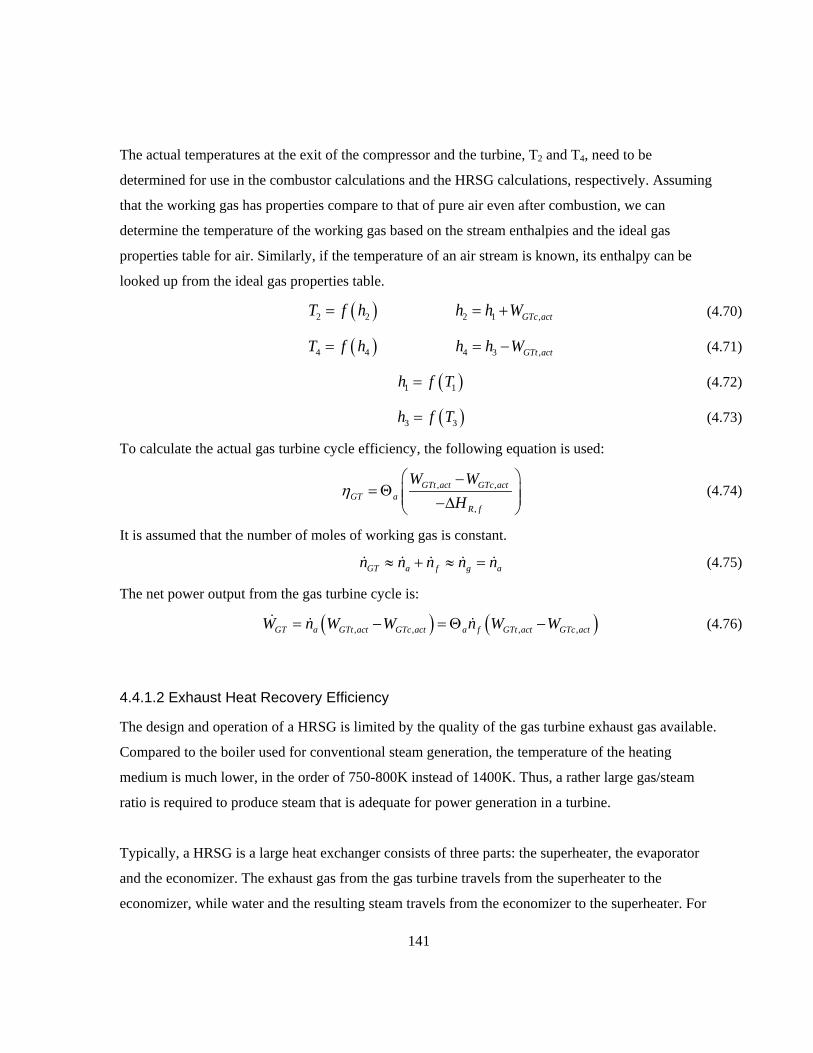
The actual temperatures at the exit of the compressor and the turbine, T2 and T4, need to be
determined for use in the combustor calculations and the HRSG calculations, respectively. Assuming
that the working gas has properties compare to that of pure air even after combustion, we can
determine the temperature of the working gas based on the stream enthalpies and the ideal gas
properties table for air. Similarly, if the temperature of an air stream is known, its enthalpy can be
looked up from the ideal gas properties table.
( )2 2 2 1 , GTc actT f h h h W= = + (4.70)
( )4 4 4 3 , GTt actT f h h h W= = − (4.71)
( )1 1h f T= (4.72)
( )3 3h f T= (4.73)
To calculate the actual gas turbine cycle efficiency, the following equation is used:
, ,
,
GTt act GTc actGT a
R f
W WH
η −
= Θ −∆ (4.74)
It is assumed that the number of moles of working gas is constant.
GT a f g an n n n n≈ + ≈ = (4.75)
The net power output from the gas turbine cycle is:
( ) ( ), , , ,GT a GTt act GTc act a f GTt act GTc actW n W W n W W= − = Θ −
(4.76)
4.4.1.2 Exhaust Heat Recovery Efficiency
The design and operation of a HRSG is limited by the quality of the gas turbine exhaust gas available.
Compared to the boiler used for conventional steam generation, the temperature of the heating
medium is much lower, in the order of 750-800K instead of 1400K. Thus, a rather large gas/steam
ratio is required to produce steam that is adequate for power generation in a turbine.
Typically, a HRSG is a large heat exchanger consists of three parts: the superheater, the evaporator
and the economizer. The exhaust gas from the gas turbine travels from the superheater to the
economizer, while water and the resulting steam travels from the economizer to the superheater. For
141

this model, it is assumed that there is no pressure drop within the HRSG and all parts are operating at
pressure. 7p . The temperature at which water is evaporated is the corresponding saturation
temperature. 7,satT .
Water is first pre-heated to a temperature slightly below the saturation temperature in the economizer.
Then, in the evaporator, water is heated to the saturation temperature and completely boiled, to exist
as a saturated vapor of the same temperature. Finally, water is heated to a temperature above the
saturation temperature, resulting in superheated steam (Figure 4.17).
The temperature difference between the saturation temperature and that of the exiting exhaust gas is
known as the pinch temperature; it is an important design parameter. Another parameter is the
temperature difference between the saturation temperature and that of the entering water, known as
the approach temperature. It is important to specify those temperatures, so that at no point during the
heat transfer, the temperature of the exhaust gas crosses the temperature of the heated steam. Once the
pinch and approach temperatures have been set, the ratio between the steam and exhaust gas flows
inside the HRSG can be determined as below (molar enthalpies are written as function of
temperature):
''4 7,pinch satT T T= − (4.77)
'7, 6approach satT T T= − (4.78)
( ) ( )( ) ( )
4 4
7 6
'''
g gs
a v w
h T h TnSGRn h T h T
−= =
−
(4.79)
4''4
7'6
T : Gas turbine exhaust temperature, K
T : Temperature of gas leaving evaporator, KT : Steam turbine inlet temperature, K
T : Temperature of water entering evaporator, K
142

Figure 4.17 Temperature profile along the HRSG
The HRSG heat exchanger is designed for the design value of gas turbine exhaust temperature (T4),
during part-load operations (2 ,0, H f f ratedc n n> < ), it is possible that exhaust temperature drops
below the rated value. Decreased exhaust temperature then leads to decreased steam turbine
efficiency, for the steam temperature in the Rankine cycle is reduced.
4.4.1.3 Steam Turbine Efficiency
The steam turbine in a CCGT operates as a closed Rankine cycle. In an ideal Rankine cycle, the
working fluid, water, first undergoes isentropic compression through a pump, then heat addition at
constant pressure occurs in a heat exchanger, followed by isentropic expansion in the turbine. Finally,
the used steam is condensed to water and resumes the cycle. Given that this is a closed cycle, the flow
rate of working fluid sn is the same throughout. The maximum theoretical efficiency of an ideal
Brayton cycle is the Carnot efficiency:
Tem
pera
ture
Length Along HRSG
T4
T5
T7
T6
Tsat
Steam
Superheater Evaporator Economizer
143

9,,
7,
1 satST th
sat
TT
η = − (4.80)
However, because of practical concerns, the Rankine cycle is different from the Carnot cycle in that
the hot stream used for heat exchange with steam is cooled more extensively, and the used steam is
condensed fully into a liquid prior to pumping. Assuming a turbine and pump efficiency of 90%, the
actual efficiency of the Rankine cycle plant can be determined as follows:
, ,,
STt act STp actST act
ST
W WH
η−
=
(4.81)
( ), 7 8,STt act STt sW h hη= − (4.82)
( )9 6 9
,STp actSTp
v p pW
η−
= (4.83)
( )7 6ST sH n h h= −
(4.84)
At the exit of the condenser (state 9), the working fluid is assumed to be in the state of saturated
liquid, so that its enthalpy can be located using the specified pressure of the stream.
9 9 9,( , )sath f p T= (4.85)
At the exit of the pump (state 6), the temperature of the working fluid remains the same as before,
only the pressure has changed because of the work done by the pump.
( )6 6 6 6 9,, sath f p T T T= = (4.86)
At the exit of the turbine (state 8), the working fluid is a saturated mixture containing both vapor and
liquid. The steam quality can also be determined from the saturation pressure of the turbine inlet
stream, assuming isentropic expansion:
( ) ( ) ( )8, 1 8 2 7 3 7 7,sh f s f s f p T= = = (4.87)
It is assumed that, since constant heat addition and rejection is taking place, 6 7p p= and. 8 9p p= .
Liquid water is assumed to be incompressible, so 9v 9v is considered a constant. The enthalpy of the
heat exchanger outlet (state 6) is coupled to the enthalpy in the gas turbine exhaust stream through the
use of the heat recovery steam generator.
144

The net power output from the gas turbine cycle is:
( ), ,ST s STt act STp actW n W W= −
(4.88)
CC GT STW W W= + (4.89)
For the design case (100% load and natural gas fuel), the ratio of air to fuel flow rate is a fixed
number. But, for off-design operating conditions (part-load or use of hydrogen-enriched fuel); where
the heat of reaction is lower than the design value, it is necessary to vary the ratio of air to fuel airΘ
in order to maintain the temperature of the combustion gas T3. Because, as demonstrated in the
section above, the temperature of working gas from the gas turbine directly impacts the efficiency of
the steam turbine cycle. But, the ratio needs to follow certain constraints: it is known that gas turbines
can operate with reduced air flow, as long as the air flow maintained above 85% of the design value.
Once that value has been reached, it is no longer possible to further reduce air flow; in consequence,
the combustion temperature starts to decline [58].
Figure 4.18 Gas turbine cycle efficiency as a function of fuel hydrogen concentration and
relative fuel rate
0%
5%
10%
15%
20%
25%
30%
35%
0% 5% 10% 15% 20%
Gas
turb
ine
cycl
e ef
ficie
ncy
Fuel hydrogen concentration
50% fuel rate 60% fuel rate70% fuel rate 80% fuel rate90% fuel rate 100% fuel rate
145

For this model, the efficiency of the gas turbine cycle is pre-determined using the relationships
outlined in 4.4.1.1; the range of input variables used is: fuel hydrogen concentration from 0% to 20%
and relative fuel flow rate from 50% to 100% (Figure 4.18). The relative fuel flow rate is defined as
the actual amount of fuel available (kmol/h) divided by the rated amount of fuel that can be used.
Once the part-load gas turbine cycle efficiency is known, it is used to find the part-load combined
cycle efficiency. The efficiency of the gas turbine cycle is dependent on the heat rate (work load) of
the gas turbine, which then influences the efficiency of the overall combined cycle with its own
change and its effect on the steam turbine cycle efficiency. The efficiency of the gas turbine cycle at
partial load (40% to 100%) and the corresponding combined cycle efficiency are presented in Figure
4.19. The logarithmic functions fitted have R2 of 0.9971 and 0.9944; they are used to calculate fixed
pairs of combined cycle and gas turbine efficiency at given load levels, which are then correlated in
Figure 4.20 is derived from the empirical relationship in Figure 4.19.
Figure 4.19 Relative efficiencies of the gas turbine cycle and of the combine cycle at part-load
conditions [58]
Combine Cycle y = 0.2017ln(x) + 1.0237
R² = 0.9944 Gas Turbine
y = 0.3422ln(x) + 1.0161 R² = 0.9971
0%
20%
40%
60%
80%
100%
0% 20% 40% 60% 80% 100%
Rel
ativ
e ef
ficie
ncy
Load
146

The correlation between the gas turbine cycle efficiency and the relative combined cycle efficiency is
used as a simple look-up function. For a R2 of 0.9912 and 27 pairs of data, the correlation is
significant for p-value <0.0005.
Figure 4.20 Relative combined cycle efficiency as a function of relative gas turbine cycle
efficiency
4.4.2 Rated power
Individual gas turbines are available a wide range of sizes, from 500 kW to 300 MW in terms of
power output. The size of the overall unit is dependent on the maximum flow rate of working fluid
that the gas turbine cycle and the steam turbine cycle are expected to process at design conditions
(100% load, natural gas as fuel). The relationship between the rated power in terms of MW is related
to the rated power expressed in terms of fuel intake rate is the following:
( ), , , ,CC rated CC rated f rated R NGW n Hη= −∆
(4.90)
( ) ( ),
CCCCGT
CC rated
W tU t
W=
(4.91)
y = -0.3993x2 + 1.2145x + 0.1874 R² = 0.9912
0%
20%
40%
60%
80%
100%
0% 20% 40% 60% 80% 100%
Rel
ativ
e co
mbi
ned
cycl
e ef
ficie
ncy
Relative gas turbine cycle efficiency
147

4.4.3 Ramp rate
Combined cycle power plants are known to have short start-up time. The following start times are
expected for different standstill periods:
• After 8 hours of standstill: 40 – 60 minutes, simplified to be 1 hour;
• After 48 hours of standstill: 80- 120 minutes, simplified to be 2 hours;
• After 120 hours of standstill: 120-170 minutes, simplified to be 3 hours.
Furthermore, combine cycle units have quick load change capability, especially the gas turbine
section. It is reported that, while operating, a CCGT plant can ramp its generation by 5-10% of its
rated output per minute [90]. In 10 to 20 minutes, it is possible for the CCGT unit to ramp up or down
completely, provided that it has not been in standstill. To simplify the overall model, the start time of
the CCGT, in the order of a few hours, is assumed to be negligible. In other words, even 100% start-
up from a standstill state is assumed to be completed within an hour.
Table 4.8 List of key variables and parameters for the CCGT model
Type Description Symbol Value Unit Ref. Input Fuel dispatched to
CCGT unit fueln kmol/h
H2 conc. in fuel 2 ,H fuelc mol. %
Output Power generated by CCGT unit CCW MW
Utilization factor CCGTU
Parameters Inlet air temperature 1T 288 K Assumed
Inlet air pressure 1p 1.01 bar Assumed
GT compressor outlet pressure
2p 15 bar Example from [91]
Air heat capacity ratio
k 1.4 Estimated
GT compressor efficiency
GTcη 84% Example from [91]
GT turbine efficiency GTtη 88% Example from
[91] Heat of reaction of natural gas
,R NGH∆ 8.04E+05 kJ/kmol Calculate from composition
Heat of reaction of hydrogen (LHV) 2,R HH∆ 2.44E+05 kJ/kmol
148

Heat capacity of air ,p ac 29.0 kJ/kmol·K Estimated
Heat capacity of natural gas
,p NGc 68.8 kJ/kmol·K Estimated
Heat capacity of H2 2,p Hc 30.0 kJ/kmol·K Estimated
Evaporator pressure/Steam turbine inlet pressure
7p 80 bar Example from [91]
Evaporator saturation temperature
7,satT 568.1 K Steam table
Pinch temperature pinchT 10 K Assumed
Approach temperature
approachT 10 K Assumed
ST turbine efficiency STtη 90% Example from
[91] Molar volume of water
9v 0.01802 m3/kmol Steam table
Pump outlet liquid pressure
6p 80 bar Example from [91]
Condenser outlet saturated liquid pressure
9p 0.08 bar Example from [91]
ST pump efficiency STpη 80% Example from
[91] Rated CCGT efficiency
,CC ratedη 52.8% Calculated
Rated GT cycle efficiency
,GT ratedη 29.8% Calculated
Rated ST cycle efficiency
,ST ratedη 32.7% Calculated
Correlation between GT efficiency and CCGT efficiency
Figure 4.20 Adapted from [58]
Rated power of CCGT ,CC ratedW From initialization MW
149

Figure 4.21 Model flow diagram for CCGT
150

4.5 Separator
The inputs that the separator model accepts is the feed dispatched toward it and the concentration of
hydrogen in the feed; the outputs expected from this model are the amount of hydrogen recovered, the
quantity of natural-gas rich adsorbate released, and the concentration of hydrogen in the adsorbate.
4.5.1 Efficiency
The efficiency of the PSA process is characterized by its recovery: the percentage of desired product
present in the mixture that is recovered after separation. For this energy hub, the recovery of
hydrogen is calculated as follows:
2 2
2 2
,
, ,
H H product productsep
H feed feed H feed
n c nn n c
η = =
(4.92)
2 2, ,H sep sep Feed H Feedn n cη= (4.93)
2
2
,
,
0.999 1H product
H sep product
c
n n
=
The adsorbate, which consists of natural gas and the hydrogen that cannot be recovered:
2,sep mix feed Hn n n= − (4.94)
( )
2 2 2
2
, ,, ,
, ,
1 sep H feed H feed HH sep mix
sep mix sep mix
n n nc
n nη− −
= =
(4.95)
The actual hydrogen recovery of any PSA process is dependent on the multicomponent adsorption
equilibrium over the temperature, pressure and concentration range of interest, the physical properties
of the gases and the adsorbent, the fluid dynamics and heat transfer inside the adsorption beds, the
feed gas conditions, and the sequence of PSA cycle steps and their duration.
The hydrogen-containing gas mixture fed to PSA processes typically contains from 60-90 mol%
hydrogen. The two most common sources of mixture are the steam-methane reformer off-gas, after
treatment in a water-gas shift reactor, and the refinery off-gas, available at 8-28 bar and at 21-38°C.
The composition of the first mixture is 70-80% H2, 15-25% CO2, 3-6% CH4, 1-3% CO, and traces of 151

N2. The second mixture contains 65-90% H2, 3-2-% CH4, 4-6% C2H6, 1-3% C3H8, and less than 0.5%
C4+ hydrocarbons. For such feed conditions, the PSA units can produce a product stream containing
98-99.999 mol% H2 at the feed gas pressure, with a hydrogen recovery of 70-90%, if state-of-the-art
commercial units are used [92]. The waste stream which contains unrecovered hydrogen and what
remains from the feed gas is released at a pressure between 1 to 2 bar. One example of such PSA
process is the 11 step cycle Polybed process.
Table 4.9 Summary of hydrogen purification PSA processes [92]
Cases Polybed Lofin Gemini
Feed H2 Conc. 77.1% 78.8% 75.4% with co-production of high purity CO2
Feed Pressure 20.7 atm 28 atm 18 atm
Feed Temp. 294 K 288 K 288 K
Gas Type SMROG ROG SMROG
Adsorbent Type Activated carbon and 5A zeolite
Silica gel and activated carbon N/A
No. of Columns 10 4 + tank 6 + 3
No. of Cycle Steps 11 9 6 or 7
Cycle Time 13.33 min 30.0 min N/A
Hydrogen Purity 99.999% 99.96% 99.999%
Hydrogen Recovery 86.0% 86.3% 87.1%
Adsorbent Productivity
34.9 ft3 feed/ft3 adsorbent/cycle
153.0 ft3 feed /ft3
adsorbent/cycle N/A
In the literature, for hydrogen/methane mixtures with lower than typical hydrogen concentration, the
following values have been reported.
152

Table 4.10 PSA Process parameters for various feed concentration [93, 94]
Cases Yang & Doong Waldron & Sircar
Feed H2 Conc. 50% 60 to 90%
Feed Pressure 34 atm 14.61 atm
Feed Temp. 298 K 303 K
Adsorbent Type Activated carbon Activated carbon
No. of Columns 1 4
No. of Cycle Steps 5 7
Cycle Time 7 min 16 min
Hydrogen Purity 93-98% 99.999%
Hydrogen Recovery 80-95% 82.5 to 85.51%
Adsorbent Productivity
36 to 66 ft3 feed /ft3 adsorbent/cycle
12.8 to 32.1 ft3 feed /ft3 adsorbent/cycle
There is evidence that the hydrogen recovery is relatively insensitive to feed composition: for
hydrogen concentration ranging from 50 to 90%, the value of hydrogen recovery has always remained
above 80%. Therefore, the hydrogen recovery of the PSA process at the energy hub used is estimated
to be 80%, regardless of feed hydrogen concentration.
4.5.2 Rated power
PSA systems can be procured from small scale plants of a few hundred Nm3/h to large scale plants
with capacity over 400,000 Nm3/h in terms of feed gas flow [70]. The output of hydrogen that is
realizable from the PSA unit with a given capacity is a function of hydrogen concentration in the feed
stream. Because the concentration of hydrogen varies in between of simulation time steps, the rated
output of hydrogen from PSA also varies.
, ,s
feed rated feed rateds
p V nRT
=
(4.96)
2 2, , ,feed rated H feed sep H ratedn c nη = (4.97)
153

Given different combination of feed concentration with process scale, the possible rated hydrogen
outputs are listed:
Table 4.11 Range of rated hydrogen output for PSA unit
Hydrogen Concentration in Feed
2% 20%
Rated Feed
Flow rate
300 Nm3/h 0.20 kmol/h 2.0 kmol/h
40,000 Nm3/h 27.08 kmol/h 270.8 kmol/h
The utilization factor of the separator can be calculated as follows:
( ) ( ),
,
sep feedsep
feed rated
n tU t
n=
(4.98)
4.5.3 Ramp rate
At this stage, to simplify the model, it is assumed that the PSA unit operates with a constant cycle
time of 30 minutes, independent of hydrogen concentration in feed and of actual PSA throughput. It is
also assumed that the PSA unit can be started completely within a single simulation time step.
Table 4.12 List of key variables and parameters for the separator model
Type Description Symbol Value Unit Ref. Input Feed to separator
feedn kmol/h
H2 conc. in feed 2 ,H feedc mol. %
Output Amount of hydrogen recovered 2 ,H sepn kmol/h
Amount of NG-rich adsorbate produced
,sep mixn kmol/h
H2 conc. in adsorbate 2 , ,H sep mixc mol. %
Utilization factor SepU
Parameters Separator hydrogen recovery
sepη 90% Estimated
Concentration of hydrogen in separated stream
2 ,H productc 0.999 1 mol. % Estimated
Rated input capacity ,feed ratedn from initialization kmol/h
154

Figure 4.22 Model flow diagram for the separator
155

4.6 Compressor
At various point in the energy hub, stand-alone compressors are used to pressurize natural gas,
hydrogen, or their mixture. In Figure 4.2, four compressors can be identified: C1, located at the
electrolyzer outlet, to compress hydrogen to the pipeline pressure of incoming natural gas; C2,
located before the injection well, to compress hydrogen enriched natural gas to wellhead pressure;
C3, located at the electrolyzer outlet, to compress hydrogen to the pressure needed for gas delivery (if
bypass of storage is an available option); C4, located at the separator outlet, to compress hydrogen to
the pressure needed for gas delivery.
The inputs accepted by a compressor sub-model are compressor inlet and outlet pressure, inlet
temperature, quantity and the hydrogen concentration of the gas to be compressed; the output
expected from the compressor model is the work that is required for the compression described. All
compressor units have identical code, only the inputs have been changed.
4.6.1 Compression Efficiency
The power required by the compressor at any given time is a function of gas flow rate and inlet/outlet
conditions. Typically, the work requirement and the effluent conditions are estimated based on inlet
conditions and the discharge pressure, assuming isothermal, adiabatic (isentropic) or polytropic
process conditions. The isothermal compression calculations represent the minimum amount of power
required, supposing that there exist an infinite number of intercoolers between stages of compression,
so that the temperature of gas is kept constant during the compression [95]. The isentropic process
assumes that no heat is added or removed from the gas during compression, and that friction is absent,
so that the entropy of the gas is kept constant during the compression. As for the polytropic
compression, it is assumed that infinite isentropic steps are conducted in series, each separated by
isobaric heat transfer, yielding the discharge temperature for the actual process. For this particular
model, isentropic conditions are assumed.
Because the compression pressure is expected to range from atmospheric pressure to hundreds of bar,
when calculating the theoretical compressor work, the deviation from the ideal gas behaviour needs to
be accounted for through the use of the compressibility factor, z, which is a function of temperature,
pressure and composition. The values of compressibility factor for the full range of temperature,
156

pressure and composition expected have already been compiled for reservoir inventory calculations.
The same values are used to populate the look-up table in the compressor model (Table 4.3)
,comp thcomp comp
comp
WP n
η= (4.99)
1
, 11
mixmix
kk
mix outcomp th in
mix in
k pW zRTk p
− = − −
(4.100)
comp,th
comp
comp
comp
mix
W : Isentropic work done by compressor, kJ/kmol
P : Actual power required by compressor, kJ/h
n : Compression gas flow rate, kmol/h
η : Compressor isentropic efficiency
k : Heat capacity
ratio of compression gas
The isentropic efficiency of typical reciprocating compressors at different pressure ratio can be
looked up from [96]. In this model, the average of the range provided is chosen as the basis of
calculations. Since the compression is simplified to be a one-stage process, scenarios with
compression ratio larger than 4 are deemed to be acceptable, with an isentropic efficiency of 87.5%.
Table 4.13 Isentropic efficiencies of reciprocating compressors
Compression Ratio Efficiencies (Engine-driven) 1.1 50-60 1.2 60-70 1.3 65-80 1.5 70-85 2.0 75-88 2.5 80-89 3.0 82-90 4.0 85-90
The heat capacity ratio, another important parameter in the determination of isentropic work needed
for compression, is also a function of mixture composition.
157

, ,
, ,
p mix i p imix
v mix i v i
c y ck
c y c= = ∑
∑ (4.101)
Figure 4.23 Heat capacity ratio as a function of hydrogen concentration in compression mixture
4.6.2 Rated Power
In this model, the compressor is not provided a fixed size at the start of the simulation. Instead, the
compressor unit is sized to accommodate the maximum compressor head that it will need to provide.
The rated compressor power is obtained by querying the maximum from the hourly indexed values of
actual compressor power required and applying a safety factor to allow for operation above design
load:
, ,max0.95comp rated compP P= (4.102)
4.6.3 Ramp Rate
It is assumed that compressors, as a gas conditioning unit, do not pose constraints in terms of ramp
rate. In other words, from one simulation time step to the next, it is assumed that the compressors can
be started-up and shut-down completely.
y = 0.03x2 + 0.0729x + 1.3062 R² = 1
1.30
1.32
1.34
1.36
1.38
1.40
1.42
0.0 0.2 0.4 0.6 0.8 1.0
Hea
t cap
acity
ratio
k
Hydrogen concentration in mixture
158

Table 4.14 List of key variables and parameters for the compressor model
Type Description Symbol Value Unit Ref. Input Gas to be
compressed compn kmol/h
H2 conc. of gas 2 ,H compc mol. %
Output Compression work requirement
compP kWh/h
Parameters Compressor isentropic efficiency
compη Table 4.13 [96]
Compressor gas heat capacity ratio
mixk Figure 4.23 Estimated
Compressibility factor correlations
Table 4.3 Aspen Plus
C1 Inlet pressure ,1inp 16 bar [68]
Outlet pressure ,1outp 60 bar Estimated
Inlet temperature ,1inT 288 K Assumed
H2 conc. of gas 2 , ,1H compc 100%
C2 Inlet pressure ,2inp ,1outP bar
Outlet pressure ,2outp whp bar
Inlet temperature ,2inT 288 K Assumed
C3 Inlet pressure ,3inp 16 bar [68]
Outlet pressure ,3outp 180 bar [97]
Inlet temperature ,3inT 288 K Assumed
H2 conc. of gas 2 , ,3H compc 100%
C4 Inlet pressure ,4inp 20 bar Assumed
Outlet pressure ,4outp 180 bar [97]
Inlet temperature ,4inT 288 K Assumed
159

Figure 4.24 Model flow diagram for the compressor
160
Chapter 5 Financial Model Development
The most important financial indicator used in this project is the net present value (NPV). NPV is
calculated by discounting the expected annual cash flow of the project into its present value. Because
the project is not simulated for the entirety of its economic lifetime, a typical annual cash flow is
estimated and projected over the lifetime of the project. The following equation is used to discount
the uniform future cash flow to its present value:
( )
111
annualn
CFNPVi i
= −
+ (5.1)
annualCF : Average annual net cash flow, $/yeari: Discount raten: Project lifetime expected, years
The estimated annual cash flow is made up of the following components: revenues from sales of
energy products (power, hydrogen, and hydrogen-enriched natural gas), expense from purchases of
energy products (natural gas, power), the inventoriable cost of purchase, the amortized capital cost for
all equipment, as well as the annual operating and maintenance costs.
( ) , ,annual annual annual inv annual OM annualCF S C I C C= − − − − (5.2)
annual
annual
inv,annual
OM,annual
S : Annual sales of energy products, $/yearC : Annual purchases of energy inputs, $/yearI : Inventoriable cost of purchase, $/yearC : Amortized capital cost, $/yearC : Annual O&M cost, $/year
5.1 Annual Sales of Energy Products
The energy hub components which produce energy products for sales are shaded in Figure 5.1: wind
power from the wind turbines, bypassed hydrogen from compressor 3, and hydrogen from the
separator via compressor 4, power delivered by the CCGT, and hydrogen-enriched natural gas from
the reservoir and/or the natural gas rich adsorbate from the separator. The value of the sales
161

transactions is determined by multiplying the hourly flow rate of the material with the corresponding
market price in place for the hour in question. The prices have been first presented in the section on
exogenous environmental variables (section 3.3).
( ) ( ) ( )wtG WtGS t P t FIT t= (5.3)
( ) ( ) ( )2 2 2 2 2, ,H H sep H b H HS t n t n t MW C = + (5.4)
( ) ( ) ( )CCGTtG CCS t W t HOEP t= (5.5)
( ) ( ) ( ),mix mix tot mix mixS t n E t C t= (5.6)
2
WtG
H
CCGTtG
mix
S : Sales of wind power to the grid, $/hS : Sales of hydrogen to customers, $/h
S : Sales of CCGT power to the grid, $/hS : Sales of mixture to customers, $/h
Since the flow rates are expressed in terms of kmol/h, whereas the market prices are often expressed
in other basis (mass or energy units), sometimes conversion is necessary. Converting a molar flow
rate to a mass flow rate is quite straightforward, but converting the molar flow rate of hydrogen
enriched natural gas into energy flow rates require the knowledge of the hydrogen concentration of
the mixture delivered:
( ) ( ) ( )2 2 2, , , ,1mix H mix tot H H mix tot NGE t c t E c t E = + − (5.7)
2
2
mix
H
NG
H ,mix,tot
E :Energy content of mixture, MMBtu/kmolE : Energy content of hydrogen, MMBtu/kmol
E : Energy content of natural gas, MMBtu/kmolc : Hydrogen concentration of mixture delivered
162

Figure 5.1 Points of sales of energy products from the energy hub
Once the revenues from all four types of sales have been calculated, the total sales are calculated by
summing the hourly values over the period of interest (2010, 2011 and 2012, respectively). In this
case, for year-based financial evaluation, the sales are summed over each of the three years simulated.
(5.8)
163

Table 5.1 List of key variables and parameters for the annual sales model
Type Description Symbol Value Unit Ref. Input Wind power delivered
to the grid WtGP MW
Hydrogen delivered by separator 2 ,H sepn kmol/h
Hydrogen delivered from bypass 2 ,H bn kmol/h
Power delivered by CCGT to the grid CCW MW
Mixture delivered to customers
,mix totn kmol/h
Hydrogen concentration of mixture delivered
2 , ,H mix totc
mol. %
Output Annual sales of energy products
annualS $/year
Sales of wind power to the grid
WtGS $/h
Sales of hydrogen to customers 2HS $/h
Sales of CCGT power to the grid
CCGTtGS $/h
Sales of mixture to customers
mixS $/h
Parameters FIT time differentiated schedule
FIT Feed-in tariff prices for different hours of the week
$/MWh [71]
Market price for H2 2HC 5 $/kg Section 3.3.4
Market price for electricity
HOEP Hourly Ontario Energy Price for 2010 to 2012, time series
$/MWh [14]
Energy content of hydrogen 2HE 0.2272 MMBtu/kmol LHV of
hydrogen Energy content of natural gas
NGE 0.7618 MMBtu/kmol Based on Table 4.2
Market price of mixture
mixC Identical to natural gas market prices
$/MMBtu Estimated in section 3.3.3
164

5.2 Annual Purchases of Energy Inputs
The annual costs incurred by the purchases of energy products consist of two components, the
purchase of natural gas from the gas grid and the purchase of electricity from the power grid. Similar
to the calculation of sales, the costs of purchases is calculated by multiplying the flow rate of the
material purchased with the corresponding market price.
Figure 5.2 Points of purchases of energy products for the energy hub
(5.9)
(5.10)
Because wind turbines are considered to be an integral part of the energy hub, wind power supplied to
the electrolyzer do not constitute a purchase, for money has not been transferred between two entities:
the operators of the wind turbines are also the operators of the energy hub. 165

The total cost of all energy purchases over a period interest is summed as follows:
( ) ( )1
t
annual Gts NGtsC C t C t= + ∑ (5.11)
Table 5.2 List of key variables and parameters for the annual purchase model
Type Description Symbol Value Unit Ref. Input Power stored from
grid GtsP MW
Natural gas injected for storage
,NG inn kmol/h
Output Annual purchase of energy inputs
annualC $/year
Cost of power from the grid
GtsC $/h
Cost of natural gas from pipelines
NGtsC $/h
Parameters Energy content of natural gas
NGE 0.7618 MMBtu/kmol Based on Table 4.2
Market price of electricity
HOEP Hourly Ontario Energy Price for 2010 to 2012, time series
$/MWh [14]
Market price of natural gas
NGC Weekly average of the Henry Hub spot price from 2010 to 2012, time series
$/MMBtu [72]
166

5.3 Inventoriable Cost of Purchase
The total purchase cost for starting material, incurred at the time of purchase, can be separated into
two components: the cost of material incurred, which represents the portion of annual purchase cost
attributable to the sales made in that year, and the inventoried purchase cost, which represents the
portion of annual purchase cost which is attributable to the inventory accrued over the year under
consideration..
annual incurredC I C= + (5.12)
incurred annualC C I= − (5.13)
annual
incurred
C : Annual purchase of energy inputs, $/yearI: Inventoriable cost of purchase, $/yearC : Incurred cost of purchase, $/year
The inventoriable cost of purchase is equivalent to the change in inventory value over the course of a
year. It is also the portion of the annual expenses that can be deducted from the annual income
statement, for not all of the material purchased is processed and delivered to the customers within the
same year. This value can be positive or negative. It is positive in the case that there is a net gain in
the value of inventory compared to the beginning of the year. It is negative if there is a net loss in the
value of inventory.
To determine the inventoriable cost of purchase, it is necessary to obtain the value of material in
storage at the beginning and end of each year.
, ,0i f ii
I II
t−
=∆
, ,0i f ii
I II
t−
=∆
(5.14)
( )2010,0 , 0res totI C t= (5.15)
( )2010, 2011,0 , 1f res totI I C t= = (5.16)
( )2011, 2012,0 , 2f res totI I C t= = (5.17)
( )2012, , 3f res totI C t= (5.18)
167

i
i,f
i,0
I : Inventoriable cost of purchase of year i, $/yearI : Cost of inventory at end of year i, $I : Cost of inventory at beginning of year i, $Δt: Period of inventory accumulation/depletion = 1 yearC ( )res,tot t : Cost of gas in storage at time t, $
At the beginning of the simulation, the value of gas in storage is estimated using the initial physical
inventory totaln totaln totaln and the estimated unit cost of the gas stored.
( ), 0 , ,0 ,0res tot mix unit totC t C n= ( ), 0 , ,0 ,0res tot mix unit totC t C n= ( ), 0 , ,0 ,0res tot mix unit totC t C n= (5.19)
mix,unit,0
tot,0
C : Initial unit cost of gas in storage, $/kmoln : Initial amount of gas in storage, kmol
Then, the value of inventory and the unit cost of store gas are updated hourly using the following
logic:
( )( ) ( ) ( ) ( )
( ) ( ) ( )( )( ) ( )2,
2
, , , s,act
,, Gts s,act
,
1 1 , if n t < 0
1 +C , if n t 0S
res tot s act mix unit
Hres totres tot NGts
H E
C t n t n tn tC t
C t C t tn t
− + −
= − + ≥
(5.20)
( ) ( )( )
,,
res totmix unit
tot
C tC t
n t= (5.21)
2
2
s,act
H ,S
H ,E
n : Actual flow rate into/out of the reservoir, kmol/hn : Amount of hydrogen stored, kmol/h
n : Amount of electrolytic hydrogen produced, kmol/h
Only a portion of the cost of grid power is allocated to the gas in storage, because not all hydrogen
produced using the electricity consumed is stored.
168

Table 5.3 List of key variables and parameters for the inventoriable purchase cost model
Type Description Symbol Value Unit Ref. Input Annual purchase of
energy inputs for year i
,annual iC $/year
Actual flow rate into/out of the reservoir
,s actn kmol/h
Cost of power from the grid
GtsC $/h
Cost of natural gas from pipelines
NGtsC $/h
Amount of hydrogen stored 2 ,H Sn kmol/h
Amount of hydrogen bypassed 2 ,H bn kmol/h
Output Inventoriable cost of purchase for year i
iI $/year
Incurred cost of purchase for year i
,incurred iC $/year
Cost of gas in storage
,res totC $
Parameters Initial unit cost of gas in storage
, ,0mix unitC 5.88 $/kmol Estimated from NGC
Initial amount of gas in storage
,0totn 2.40E+06 kmol Assumed
169

5.4 Capital Cost
The capital cost of the energy hub is determined based on the rated input or output capacity of its
constituents. Wind turbines, electrolyzers, compressors, the separator unit and the combined-cycle gas
turbine plant make up the bulk of the capital cost. For this model other components of the capital cost
are assumed to be negligible. In the case that the configuration of energy hub excludes a given
component, the component in question does not contribute to the total capital cost.
, , , , , ,inv tot W inv E inv sep inv CCGT inv comp invC C C C C C= + + + + (5.22)
Once the total capital cost value is obtained, the capital recovery factor is used to transform the total
capital investment, a one-time cash flow at the beginning of the project, into a series of constant
annuities over the course of project life. By definition, it is calculated as follows:
( )
( )1
1 1
n
n
i iCRF
i+
=+ −
(5.23)
, ,inv annual inv totC C CRF= (5.24)
5.4.1 Wind Turbines
The capital cost of wind power projects in Canada is given as a function of project rated capacity
[98]:
2008, ,
2006
$2,000,000W inv W ratedCEPCIC PCEPCI
= (5.25)
2008
2006
CEPCI : Chemical Engineering Plant Cost Index for 2008CEPCI : Chemical Engineering Plant Cost Index for 2006
A technical lifetime of 20 years is expected for wind turbines. As long as the economic lifetime of the
project falls below 20 years, it is not necessary to incur replacement costs.
5.4.2 Electrolyzers
This section to determine the capital cost of electrolyzers is adapted from [99-101]. It is known that
for hydrogen production scale ranging from 0.05kmol/h to 50kmol/h, only one unit of electrolyzer is
needed, and economies of scale is possible.
170

( )2 2
0.6156
, , , , ,224,490 2 0.05 50E inv E H rated E H RatedC n n= ≤ ≤ (5.26)
Modules of a given rating (2.7kmol/h, HySTAT-60 from Hydrogenics Corps.) have been chosen for
this model. The capital cost required for an individual unit is thus:
( )2
0.6156
, , , , ,$224,490 2E inv i E H rated iC n= (5.27)
The total capital cost for electrolyzers depend on the number of units procured:
, ,0 , ,E inv E E inv iC N C= (5.28)
The typical lifetime of alkaline electrolyzers is estimated to be 10 years. Therefore, if the economic
lifetime of the project is set to more than 10 years, replacement costs are incurred for electrolyzers in
the 10th year of operation. Replacement costs are estimated to be 50% of the original capital cost at
the time of replacement. It is discounted to its present value.
, ,0, , 10
0.5(1 )
E invE inv rep
CC
i=
+ (5.29)
, , ,0 , ,E inv E inv E inv repC C C= + (5.30)
5.4.3 Separator
The main initial investment for a PSA system consists of the purchase of the adsorption beds
(adsorbent and the vessel). Compressors are not required for feed pressurization, because reservoir
gas is available at pressures higher than 20 bar, the stated operating pressure of the adsorption
columns.
, , ,sep inv sep ads sep colC C C= + (5.31)
sep,ads
sep,col
C : Capital cost of adsorbent, $
C : Capital cost of separation columns, $
The total adsorption volume required for the separation is calculated using the values of adsorbent
productivity. The adsorbent productivity (MAR) for the operation conditions considered: 20 bar and
298 K, is approximated to be 30 volumetric units of feed per volume unit of active carbon per cycle,
or 60 volumetric units of adsorbent for an hour (2 cycles occur per hour, 30 minutes per cycle).
171

hh cycle
cycle
tMAR MARt
= (5.32)
,feed ratedads
h
VV
MAR=
(5.33)
3 3h
3 3cycle
h
cycle
3ads
feed,rated
MAR : Adsorbent productivity, Nm m h
MAR : Adsorbent productivity, Nm m cycle
t : Time in an hour = 60 mint : Duration of a cycle, min
V : Volume of adsorbent required, m
V : Rated in
3put capacity of separator, Nm /h
Then, the cost of adsorbent used in the process can be calculated using its market price ($/weight)
,sep ads ads ads adsC V Cρ= (5.34)
3ads
ads
ρ : Density of adsorbent (active carbon), kgC : Unit cost of adsorbent (active carbon), $/kg
m
The cost of the containing vessels is an important part of the overall unit cost. It is assumed that
vessels 20 ft long, and 6 ft in diameter are used. Approximating the volume of vessels as cylinders,
the number of vessels required to contain the adsorbent needed can be calculated. In order to ensure
continuous process operation, the minimum number of adsorption beds is 2. The unit cost of vessels
is computed using the Guthrie method, adjusted for its size, then updated from 1969 dollars to 2008
dollars using the Chemical Engineering Plant Cost Index (CEPCI) [102].
( )22col col colV D Lπ= (5.35)
2, 2
, 2
ads
colcol
ads ads
col col
VV
NV VroundV V
<= ≥
(5.36)
( )0.78 0.98
2008,
1969
$690 3.18 1.05 14 3
col colsep col col col col
CEPCI L DC N C NCEPCI ft ft
= = + −
(5.37)
172

3
col
col
col
col
col
V : Volume of a column, mD : Diameter of a column, mL : Length of a column, mN : Number of columns requiredC : Unit cost of column, $/column
It is assumed that the technical lifetime of the vessels as well as the adsorbent is longer than the
economic lifetime of the project; therefore, there are no replacement costs to be considered.
5.4.4 CCGT
For the range of capacity foreseen (< 200 MW), the investment cost of CCGT power plants is
estimated to be $650/kW in 2006 dollars [58]. This figure is converted to 2008 dollars as in the rest of
costing calculations:
2008, ,
2006
$650,000CCGT inv CC ratedCEPCIC WCEPCI
=
(5.38)
The technical lifetime of CCGT plants are in the order of 30 years, longer than the economic lifetime
specified for this project, therefore there is no replacement cost for the turbines.
5.4.5 Compressors
The compressor cost model in this section is based on the work of [103] on the compression costs for
carbon dioxide sequestration. The capital investment required by the compression unit is:
, ,comp inv comp rated compC P C= (5.39)
The cost factor for a range of rated capacity is shown in the figure below; as the rated capacity
increases, the per unit cost decreases because of economies of scale. It is assumed that the service life
of the compressors is longer than the life time of the project, and no replacement investment is
required.
173

Figure 5.3 Capital cost factor of compressors for different installed capacity[104]
Note that there are four compression units of different rated capacities; the calculations above are
completed for all four. The final capital cost reported includes for all units.
y = 11855x-0.286 R² = 0.8349
$0
$1,000
$2,000
$3,000
$4,000
$5,000
$6,000
$7,000
$8,000
$9,000
$10,000
0 5,000 10,000 15,000 20,000 25,000 30,000
Inst
alle
d co
st ($
/kW
)
Rated capacity of compressor (kW)
174

Table 5.4 List of key variables and parameters for the capital cost model
Type Description Symbol Value Unit Ref. Input Rated capacity of
wind turbines ,W ratedP MW
Number of electrolyzer units
EN
Rated input capacity of separator ,feed ratedV Nm3/h
Rated capacity of CCGT ,CC ratedW MW
Rated capacity of compressor
,comp ratedP kW
Output Total capital cost required
,inv totC $
Amortized capital cost
,inv annualC $/year
Capital cost of wind turbines
,W invC $
Capital cost of electrolyzers
,E invC $
Capital cost of the separator
,sep invC $
Capital cost of the CCGT
,CCGT invC $
Capital cost of compressors
,comp invC $
Parameters Discount rate i 8% Assumed Expected project lifetime
n 20 years Estimated
CEPCI index for 2008
2008CEPCI 575.4
CEPCI index for 2006
2006CEPCI 499.6
CEPCI index for 1969
1969CEPCI 119
Unit cost factor for wind turbines
2E+06 $/MW [98]
Rated capacity of electrolyzer unit 2, , ,E H rated in 2.7 kmol/h [68]
Adsorbent productivity
cycleMAR 30 Nm3/(m3-cycle) Estimated
Duration of a separation cycle
cyclet 30 min Estimated
Density of adsorbent adsρ 481 kg/m3 [64]
175

Unit cost of adsorbent
adsC 1 $/kg Estimated
Diameter of a column
colD 1.83 m [94]
Length of a column colL 6.1 m [94]
Correlation between column volume and column unit cost
[102]
Unit cost factor for CCGT
6.5E+05 $/MW [58]
Unit cost factor for compressors
See Figure 5.3 $/kW [104]
176

5.5 Operating and Maintenance Cost
Operating and maintenance cost for the energy hub is divided into two types: fixed and variable.
Fixed maintenance cost is assumed to be a percentage of the annual capital cost:
, ,OM fixed OM inv annualC R C= (5.40)
OM inv,annualR :Fixed operating cost ratio, % of C
The variable operating cost is mainly attributed to the consumption of energy by reciprocating
compressors used on-site. Reciprocating compressor can have two types of driver: natural gas engines
or electric motors. It is assumed that the compressors used at the energy hub are powered by natural
gas engines. The energy consumption of the compressors is converted expressed in terms of natural
gas consumption, through the use of conversion factors.
,comp NG compNG
GPRP PE
= (5.41)
comp,NG
comp
NG
P : Natural gas required by compressors, kmol/h
P : Power requirement of compressors, kWh/h
GPR: Gas energy required per unit of electrical energy, MMBtu/kWhE : Energy content of natural gas, MMBtu/kmol
The cost of energy consumed by compressors is calculated as follows:
( ) ( ) ( ), ,comp E comp NG NGC t P t C t= (5.42)
The annual operating and maintenance is the sum of the fixed cost and the annual variable cost:
( ), , ,1
t
OM annual OM fixed comp EC C C t= +∑ (5.43)
177

Table 5.5 List of key variables and parameters for the O&M cost model
Type Description Symbol Value Unit Ref. Input Amortized capital
cost ,inv annualC $/year
Power requirement of compressors
compP kWh/h
Output Fixed annual O&M cost
,OM fixedC $/year
Energy cost for compression
,comp EC $/h
Annual O&M cost ,OM annualC $/year
Parameters Fixed operating cost ratio
OMR 4% % of ,inv annualC
Gas energy required per unit of electrical energy
GPR 0.010 MMBtu/kWh [96]
Energy content of natural gas
NGE 0.7618 MMBtu/kmol Based on Table 4.2
178

Chapter 6 Emission Model Development
The emission model complements the financial model by assessing the environmental performance of
the energy hub. The key indicator used is the net emissions (incurred or mitigated) due to the
operation of the energy hub during the simulated year.
6.1 Net Emissions
The carbon dioxide emissions associated with the operation of the energy hub are divided into two
types: the emissions which are incurred during the operation of the energy hub, and emissions which
are mitigated by the operation of the energy hub. The net amount of emissions mitigated is given by
the following difference:
2, 2, 2,CO net CO incurred CO mitigatedm m m= − (6.1)
2,
2,
2,
CO net 2
CO incurred 2
CO mitigated 2
m : Net emissions, kg CO /year
m : Emissions incurred, kg CO /year
m : Emissions mitigated, kg CO /year
A positive net emissions value means that more carbon dioxide have been emitted because of the
operation of the energy hub; a; a negative value means that, overall, carbon emissions have been
mitigated due to the operation of the energy hub.
6.2 Emissions Incurred
The carbon dioxide associated with the operation of the energy hub is attributed to five sources: on-
site use of natural gas driven compressors for gas compression, consumption of grid-generated
electricity, electricity generation from on-site wind turbines, on-site use of the CCGT for energy
recovery, and the off-site use of hydrogen-enriched natural gas, once it reaches the end-users through
the distribution pipelines.
2 2 2 2 2 2, , , , , ,CO incurred CO comp CO G CO W CO CCGT CO mixm m m m m m= + + + + (6.2)
179

6.2.1 Gas Compression
The amount of compressor work required is known from the simulations. It is still necessary to
calculate the emissions associated with this known compression duty. Assuming that all compressors
present at the energy hub have natural gas-driven engines, the following conversion factors are used:
( )2 , ,CO comp NG comp comp
NG
GPRn n P tE
= = ∑ (6.3)
2 2 2, ,CO comp CO comp COm n MW= (6.4)
6.2.2 Electrolyzer Power Supply
The carbon dioxide emitted by grid-connected generators that supply the electrolyzer is a function of
two variables. First of all, the emission factor of grid-supplied power, which is function of time and
estimated as described in section 3.3.1. Secondly, the emissions of grid-connected generators that can
be attributed to the operation of the energy hub are limited to the amount of grid power delivered to
the electrolyzer. Obviously, the absolute value of carbon dioxide emitted from all grid-connected
generators is a much higher value, but only the portion that is consumed by the energy hub is counted
in these calculations.
( ) ( )2,GCO G Gtsm EF t P t= ∑ (6.5)
The carbon dioxide emissions associated with wind power generation from existing life cycle analysis
is low but non-negligible. Unlike the emission factor for the grid which is transient, the emission
factor for wind turbines is assumed to be a number that is constant over the lifetime of the turbine.
Note that the power generated by wind turbines is not only used to supply the electrolyzer ( wtsP wtsP
wtsP ), but it may also be delivered to the grid directly wtGP ( wtGP wtGP ) when market conditions are
favourable.
( )2,CO W W Wm P t EF= ∑ (6.6)
( ) ( ) ( )W wts wtGP t P t P t= + (6.7)
180

6.2.3 On-Site CCGT Generation
Assuming 100% combustion within the gas turbine, the number of moles of carbon dioxide produced
by the combustion of fuel is the same as the number of moles of natural gas consumed. Upon
combustion, hydrogen does not form carbon dioxide.
( ) ( ) ( ){ }2 2 2, ,1CO CCGT H fuel fuel COm t c t n t MW = − ∑ (6.8)
6.2.4 HENG Mixture Consumption
Another important source of carbon emissions come from the use of hydrogen-enriched natural gas
mixture once it has reached the end-users. Similarly to fuel combustion at the on-site CCGT, only the
natural gas contained in the mixture contributes to carbon dioxide formation, whereas the hydrogen
added produces mainly water vapour as a combustion product.
( ) ( ){ }2 22, ,,1CO mix mix tot COH mix tm c n t MW = − ∑ (6.9)
6.3 Emissions Mitigated
On the other hand, carbon dioxide emissions which are mitigated due to the operation of the energy
hub can also be attributed to three sources. The delivery of electrolytic hydrogen displaces the need
for hydrogen produced via steam methane reforming. The delivery power from the mixture-fired
CCGT allows for the displacement of emissions from other gas turbines which run on pure natural
gas. Finally, the gas end-users no longer consume pure natural gas, since they are now supplied with
the hydrogen-enriched gas mixture.
2 2 2 2, , , ,CO mitigated CO SMR CO fuel CO NGm m m m= + + (6.10)
6.3.1 Hydrogen from Steam Methane Reforming
The amount of electrolytic hydrogen delivered displaces the same amount of hydrogen produced via
the traditional steam methane reforming process. The carbon dioxide emissions associated with unit
production of hydrogen via SMR is documented in the literature [105].
( ) ( )2 2 2 2, , ,CO SMR H b H sep H SMRm n t n t MW EF = + ∑ (6.11)
181

6.3.2 Gas-Fired CCGT Generation
It is assumed that, in the case that the energy hub did not operate, the power generated by the on-site
CCGT plant would still be delivered to the grid, but by a competing CCGT operator that supplies the
gas turbine with pure natural gas.
( )2 2,CO fuel fuel COm n t MW = ∑ (6.12)
6.3.3 Natural Gas Consumption
Analogous to the section above, it is assumed that, in the case that the energy hub did not operate,
then the off-site customers would have used pure natural gas instead of hydrogen-enriched natural
gas. The emissions that would have been produced from the combustion of natural gas are:
( )2 2, ,CO NG mix tot COm n t MW = ∑ (6.13)
Table 6.1 List of key variables and parameters for the emission model
Type Description Symbol Value Unit Ref. Input Power requirement
of compressors compP kW
Power stored from grid
GtsP MW
Wind power generated
WP MW
Fuel dispatched to CCGT
fueln kmol/h
H2 concentration of fuel 2 ,H fuelc mol. %
Mixture delivered to client
,mix totn kmol/h
H2 concentration of mixture delivered 2 , ,H mix totc mol. %
Hydrogen delivered by separator 2 ,H sepn kmol/h
Hydrogen delivered from bypass 2 ,H bn kmol/h
Output Net emissions 2,CO netm kg CO2/year
Emissions incurred 2,CO incurredm
kg CO2/year
182

Emissions mitigated 2,CO mitigatedm
kg CO2/year
Emissions from gas compression 2 ,CO compm kg CO2/year
Emissions from grid power generation 2 ,CO Gm kg CO2/year
Emissions from wind power generation
2 ,CO Wm kg CO2/year
Emissions from on-site CCGT power generation
2 ,CO CCGTm kg CO2/year
Emissions from off-site use of mixture 2 ,CO mixm kg CO2/year
Emissions displaced from SMR hydrogen 2 ,CO SMRm kg CO2/year
Emissions displaced from on-site CCGT fuel use
2 ,CO fuelm kg CO2/year
Emissions displaced from off-site NG use 2 ,CO NGm kg CO2/year
Parameters Gas energy required per unit of electrical energy
GPR 0.010 MMBtu/kWh [96]
Energy content of natural gas
NGE 0.7618 MMBtu/kmol Based on Table 4.2
Emission factor of grid power in Ontario
GEF Figure 3.8 kg CO2/MWh Estimated from [106] and Ontario demand
Emission factor of wind power
WEF 19 kg CO2/MWh [106]
Emission factor for hydrogen production via SMR
SMREF 10.6 kg CO2/kg H2 [105]
Molar mass of H2 2HMW 2 kg/kmol
Molar mass of CO2 2COMW 44 kg/kmol
183

Chapter 7 Scenario Generation
In order to understand the impact of proposed underground storage of hydrogen, one base case
scenario and four additional scenarios are generated, each focusing on one particular use of the
hydrogen storage technology.
7.1 Base Case Scenario: Underground Gas Storage
The base case scenario describes the operation of an underground gas storage facility without the
production and storage of hydrogen. Conventionally, natural gas is injected into UGS facilities from
April through October and withdrawn from November through March, completing a gas storage cycle
in a year. The underlying driving force is the typical natural gas profile: low prices during summer
and higher prices during winter, the heating season. But, in recent years, the seasonal variation in
natural gas prices is dwarfed by the year-to-year variation. In order to factor in the effect of year-to-
year natural gas price fluctuation on UGS facilities, a three calendar year simulation time frame is
chosen. The results obtained from the base case scenario allows one to differentiate between the
variability inherent to UGS facilities and the effect of underground storage of hydrogen, which is
performed in addition to regular UGS operations.
7.1.1 Summary
In this scenario, the energy hub is operated as a conventional natural gas storage facility, thus it is
simplified to its core component: the storage reservoir (and compressor required for gas injection).
The updated diagram illustrating the configuration of the base case scenario is shown below:
Table 7.1 Configuration and capacity of energy hub components for the base case scenario
Component Status Rated Capacity
Reservoir ON 6.1-7.6 MMscf
Electrolyzers OFF N/A
Wind Turbines OFF N/A
CCGT OFF N/A
Separator OFF N/A
184

Figure 7.1 Model scope for the base case scenario
Table 7.2 Summary of decision point logic for the base case scenario
Description Action D1 Reservoir operation
regime Inject when the NG market price is low; withdrawal when the NG market price is high
D2 Electrolyzer power supply
N/A
D3 Hydrogen bypass N/A
D4 NG/H2 blending Set NG stored to injectability limit
D5 Mixture dispatch Set NG produced to deliverability limit
D6 Separator recycle N/A
185

7.1.2 Decision Point Model Logic
Figure 7.2 Reservoir operation decision point (D1) for the base case scenario
The key decision point present in this scenario is D1, depicted below: the reservoir enters injection
mode whenever the market of natural gas is lower than the threshold value by $0.20. On the other
186

hand, whenever the market price of natural gas is $0.20 higher than the threshold value, the reservoir
enters withdrawal mode. When the prices are equal, the reservoir remains in shut-in mode.
For this case, the threshold price used is the moving average of the Henry Hub spot price for a 26
weeks window. The moving average value is preferred over a static value, because, for the three years
selected as basis years of simulation (2010-2012), the price of natural gas has changed significantly.
Compared to its seasonal fluctuations; a static threshold value is incapable of reflecting this change in
the market.
Figure 7.3 Natural gas market price and its 26 weeks moving average for years 2010-2012
The deliverability and injectability are outputs of the reservoir model, upon receiving and interpreting
the dispatch order made by D1. Based on the inventory level and the limits placed on wellhead
pressure, the wellhead pressure is adjusted, and the corresponding flow rate limit is determined. It is
possible for the reservoir to remain in shut-in (deliverability/injectability~ 0) even when there is
Q4 2009
0123456
0
Measure Names
187

dispatch order to inject or to withdrawal, if it violates a given physical constraint that is associated
with the storage reservoir.
At D4, the amount of natural gas stored is set to be equal to the injectability of the reservoir at that
given hour. Since no hydrogen is produced, the concentration of hydrogen in the injected stream is
always zero.
Figure 7.4 Gas blending decision point (D4) for base case scenario
188

For D5, the amount of natural gas delivered to the grid is set to be equal to the deliverability for the
reservoir at that given hour.
Figure 7.5 Mixture dispatch decision block (D5) for the base case scenario
189

7.2 Mid-Term Scenario: Hydrogen Injection
This second scenario is different from the other non-base case scenarios, for it simulates conditions
which are likely to be in place a short time after the implementation of the underground storage of
hydrogen: hydrogen is produced and injected into the natural gas storage system in relative small
proportions (Figure 1.6). The hydrogen injection scenario is a mid-term scenario because, compared
to the three later scenarios, it requires relatively little capital investment.
7.2.1 Summary
Compared to the previous scenario, electrolyzers are added as another key component of the energy
hub, bring with it connectivity to the power grid and to demand for hydrogen (Table 1.3).
Table 7.3 Configuration and capacity of energy hub components for the hydrogen injection
scenario
Component Status Rated Capacity
Reservoir ON 6.1-7.6 MMscf
Electrolyzers ON 8.7 MW or 30 units
Wind Turbines OFF N/A
CCGT OFF N/A
Separator OFF N/A
190
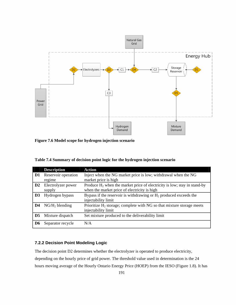
Figure 7.6 Model scope for hydrogen injection scenario
Table 7.4 Summary of decision point logic for the hydrogen injection scenario
Description Action D1 Reservoir operation
regime Inject when the NG market price is low; withdrawal when the NG market price is high
D2 Electrolyzer power supply
Produce H2 when the market price of electricity is low; stay in stand-by when the market price of electricity is high
D3 Hydrogen bypass Bypass if the reservoir is withdrawing or H2 produced exceeds the injectability limit
D4 NG/H2 blending Prioritize H2 storage; complete with NG so that mixture storage meets injectability limit
D5 Mixture dispatch Set mixture produced to the deliverability limit
D6 Separator recycle N/A
7.2.2 Decision Point Modeling Logic
The decision point D2 determines whether the electrolyzer is operated to produce electricity,
depending on the hourly price of grid power. The threshold value used in determination is the 24
hours moving average of the Hourly Ontario Energy Price (HOEP) from the IESO (Figure 1.8). It has 191

been found that the HOEP is a good indicator of the degree of demand for electricity in the Ontario
market. In this scenario, it is estimated that, whenever the HOEP is lower than its daily moving
average, the demand for electricity is lower than average. Thus it is preferable to use grid power to
supply electrolytic hydrogen production, when surplus baseload generation is more plentiful. Vice
versa, when HOEP is higher than its daily moving average, the electrolyzers are in stand-by as to not
increase electricity demand during those hours. This practice ensures that the electrolyzer is operated
daily during the off-peak hours.
This second scenario shares the same decision point logic with the base case scenario at D1 and D5:
reservoir dispatch is based on natural gas prices, and once the reservoir has been dispatched to
withdrawal, all the gases that can be produced is directed toward distribution via the natural gas
distribution network. This scenario also contains two new decision points (D2 and D3) and an altered
version of D4, for hydrogen is present (Figure 1.7, Figure 1.9 and Figure 1.10).
192

Figure 7.7 Electrolyzer power supply decision point (D2) for the hydrogen injection scenario
Figure 7.8 Ontario power price and its 24 hours moving average for years 2010-2012 193

The decision D3 determines whether the hydrogen produced by the electrolyzer is sent to storage. As
input, it requires the knowledge of the reservoir injectability/deliverability and the flow rate of
hydrogen produced. Hydrogen is sent for storage if it has been produced and if the reservoir is
accepting injected gas. In the case that the hydrogen produced exceeds the injectability of the
reservoir, or in the case that the reservoir is producing gas from storage, the portion of hydrogen that
cannot be injected is assumed to be absorbed by local hydrogen demand, immediately. This
assumption can be verified by examining the amount of hydrogen thus consumed from simulation
results.
Figure 7.9 Hydrogen bypass decision point (D3) for the hydrogen injection scenario
194

The penultimate decision point, D4, determines how much natural gas is blended with the hydrogen
that is to be injected. In this scenario, the amount of natural gas alongside hydrogen is calculated
based on the injectability of the reservoir. It is set up so that the combined mixture fulfills the
injectability limit exactly, so that the maximum amount of gas is injected into the reservoir during its
operations. At decision point D5, as in the scenario before, the amount of mixture delivered
remains matched to the deliverability limit (Figure 1.5).
Figure 7.10 Gas blending decision point (D4) for hydrogen injection scenario
195

7.3 Long-Term Scenario: Reduction of Surplus Baseload (SGB) Generation
The surplus baseload generation reduction scenario is the first of three long-term scenarios. It differs
from the hydrogen injection scenario in that an on-site combined cycle gas turbine plant is included in
the energy hub, so that the stored energy can be recovered in the form of electric power at the energy
hub (Figure 1.11 and Table 1.5). This configuration allows the energy hub operators to store
electricity from the grid and to deliver electricity to the grid at the same physical location.
7.3.1 Summary
In order to be able to compare scenarios in a meaningful way, the rated capacity of the electrolyzer
unit has been maintained to be the same as in the mid-term scenario at 8.7 MW. But, realistically, the
full absorption of the surplus baseload generation in Ontario will require a much larger capacity. In
that case, the number of energy hubs such as the one described within this scenario can be multiplied
to scale up.
Table 7.5 Configuration and capacity of energy hub components for the SBG reduction
scenario
Component Status Rated Capacity
Reservoir ON 6.1-7.6 MMscf
Electrolyzers ON 8.7 MW or 30 units
Wind Turbines OFF N/A
CCGT ON 40 MW
Separator OFF N/A
196

Figure 7.11 Model scope for the SBG reduction scenario
For long-term scenarios, the dispatch logic for the reservoir and for the energy hub as a whole is
significantly different from the base case.
Table 7.6 Summary of decision point logic for the SBG reduction scenario
Description Action D1 Reservoir operation
regime Inject when the demand for electricity is low; withdrawal when the demand for electricity is high
D2 Electrolyzer power supply
Produce H2 when the demand for electricity is low; stay in stand-by when the demand for electricity is high
D3 Hydrogen bypass Bypass if the reservoir is withdrawing or H2 produced exceeds the injectability limit
D4 NG/H2 blending Prioritize H2 storage; complete with NG so that mixture storage meets injectability limit
D5 Mixture dispatch Set mixture produced to deliverability limit; prioritize supplying CCGT before sending the mixture to the NG distribution pipelines
D6 Separator recycle N/A
197

7.3.2 Decision Point Modeling Logic
To begin, at decision point D1, when deciding whether to inject or withdrawal from the reservoir, the
triggering signals are no longer the natural gas market price. Instead, the hourly demand for electricity
in the province is compared to a threshold value, which triggers hydrogen production. This is
followed by injection when electricity demand is low, mixture withdrawal when demand is high
(Figure 1.12).
Figure 7.12 Reservoir operation decision point (D1) for the SBG reduction scenario
The threshold value used in this scenario is the one year moving average of Ontario-wide electricity
demand (Figure 1.13). 198

Figure 7.13 Electricity demand in Ontario and its one-year moving average for 2010-2012
At decision point D2, the electrolyzer dispatch is also modified to be triggered by deviation from
electricity demand instead of by deviation from electricity market prices (Figure 1.14). At D3 and D4,
the logic directing the bypassing of hydrogen and the blending of hydrogen with natural gas,
respectively, has remained unchanged. The maximum limit of the quantity of hydrogen and natural
gas stored is set by the injectability limit, with priority for hydrogen (Figure 1.9 and Figure 1.10).
Q1 2010
0K2K4K6K8K10K12K14K16K18K20K22K24K26K
0K
Measure Names
199

Figure 7.14 Electrolyzer power supply decision block (D2) for the SBG reduction scenario
Finally, once the stored mixture is withdrawn following signals of higher demand, it is necessary to
determine its dispatch to different product delivery pathways. The hydrogen-enriched natural gas can
be delivered as is through natural gas pipelines and then consumed off-site, or it can be consumed on-
site to fuel the CCGT plant. Since the fuel intake of the CCGT plant is much smaller than the average
deliverability of the reservoir, the nominal need of the gas turbine is met first, and the remainder of
the mixture retrieved is routed toward the gas distribution network (Figure 1.15).
200

Figure 7.15 Mixture dispatch decision block (D5) for the SBG reduction scenarioLong-Term
Scenario: Integration of Wind Power 201

In this second long-term scenario, on-site or near-by wind turbines are added to the energy hub
components present in the previous scenario. The wind turbines are included within the boundary of
the energy hub, because it is assumed that they have the same proprietaries and operators as the rest
of the energy hub. In keeping with the previous scenarios, the rated capacity of the electrolyzer is
maintained at the same level (Table 1.7), and the wind turbines have been sized to match.
7.3.3 Summary
Figure 7.16 Model scope for the wind power integration scenario
202

Table 7.7 Configuration and capacity of energy hub components for the wind power integration
scenario
Component Status Rated Capacity
Reservoir ON 6.1-7.6 MMscf
Electrolyzers ON 8.7 MW or 30 units
Wind Turbines ON 10 MW or 5 units
CCGT ON 40 MW
Separator OFF N/A
The active decision points involved in the wind power integration scenario is the same as in the SBG
reduction scenario. D3, D4, D5 remained identical in content, whereas D1 and D2 contain altered
logic.
Table 7.8 Summary of decision point logic for the wind power integration scenario
Description Action D1 Reservoir
operation regime Inject when the demand for wind power is low; withdrawal when the demand for wind power is high
D2 Electrolyzer power supply
Produce H2 when the demand for wind power is low; stay in stand-by when the demand for wind power is high; if wind is not enough for electrolyzers to produce at rated capacity, purchase power from the grid
D3 Hydrogen bypass
Bypass if the reservoir is withdrawing or H2 produced exceeds the injectability limit
D4 NG/H2 blending Prioritize H2 storage; complete with NG so that mixture storage meets injectability limit
D5 Mixture dispatch Set mixture produced to deliverability limit; prioritize supplying CCGT before sending the mixture to the NG distribution pipelines
D6 Separator recycle
N/A
7.3.4 Decision Point Modeling Logic
At the first decision point (D1), reservoir is dispatched to inject when the demand for wind power is
low, and to withdrawal when the demand for wind power is high. The indicator used to gauge the
demand for power form the wind turbines is the time-differentiated FIT contract price, which
differentiates between peak and off-peak hours in a week (Figure 1.17)
203

Figure 7.17 Reservoir operation decision point (D1) for the wind power integration scenario
204

Figure 7.18 Electrolyzer power supply decision point (D2) for the wind power integration
scenario
As for D2, the decision to operate the electrolyzers or not is also driven by the perceived demand for
wind power. The variability of wind also needs to be addressed here: depending on the local wind 205

speed, the wind power produced by the turbines may be insufficient to support the electrolyzers to run
at their rated capacity, or the wind power available may exceed the rated capacity of the electrolyzers.
In such cases, decisions are made to supplement the power supply with electricity purchased from the
grid, or to sell wind power exceeding the capacity of electrolyzers to the grid, respectively.
Decision points D3, D4 and D5 have the same logic as in the previous scenario: hydrogen storage is
prioritized when injection is possible, injection and withdrawal flow rates area always set to the value
of injectability/deliverability limits, and CCGT operation is prioritized when withdrawal is possible.
206

7.4 Long-Term Scenario: Meeting Large Hydrogen Demand
In the last of the three long-term scenarios, it is assumed that energy is mainly used for hydrogen
production, and that the storage reservoir is transitioning toward a pure hydrogen storage facility. In
this case, only hydrogen is injected to the reservoir. Assuming that natural gas with relatively high
percentages of hydrogen is produced from the reservoir, the main pathway for energy recovery is the
purification of produced gas through a PSA separator. The natural gas rich “waste stream” from the
separator contains little hydrogen; it is subsequently distributed through the natural gas distribution
system.
7.4.1 Summary
Figure 7.19 Model scope for the large hydrogen demand scenario
207

Table 7.9 Configuration and capacity of energy hub components for the large hydrogen
demand scenario
Component Status Rated Capacity
Reservoir ON 6.1-7.6 MMscf
Electrolyzers ON 26.1 MW or 90 units
Wind Turbines OFF N/A
CCGT OFF N/A
Separator ON 40,000 Nm3 feed
The rated capacity of the separator is expressed in terms of feed, for the rated output is dependent on
the concentration of hydrogen in the feed stream, which is currently unknown.
Table 7.10 Summary of decision point logic for the large hydrogen demand scenario
Description Action D1 Reservoir
operation regime Inject when there is no hydrogen demand and hydrogen is produced; withdrawal when there is hydrogen demand but no production; standby for other situations
D2 Electrolyzer power supply
Produce hydrogen when market price of electricity is low, remain in standby when price of power is high (same as D2.2)
D3 Hydrogen bypass Bypass hydrogen if there is hydrogen demand
D4 NG/H2 blending Prioritize H2 storage; no natural gas injected
D5 Mixture dispatch Set mixture produced to rated feed capacity of the separator if there is production; separation is the exclusive pathway
D6 Separator recycle Waste stream from separator supplied as mixture
208

7.4.2 Decision Point Modeling Logic
Figure 7.20 Reservoir operation decision point (D1) for the large hydrogen demand scenario
A key difference of the large hydrogen demand scenario compared to the others is that the demand for
hydrogen is considered to be fixed in time (hydrogen delivered during some hours are purchased,
instead of being fully flexible (hydrogen delivered at all hours are purchased). Here, the main purpose
209

of the storage reservoir is to provide a source of hydrogen supply when it is not being produced from
the electrolyzer, as the demand for hydrogen arises (Figure 1.20). If hydrogen has been produced
while there is no demand for hydrogen, the reservoir is activated for injection so the production can
be stored. The bypass decision block reflects the priority given to meeting hydrogen demand (Figure
1.21).
Figure 7.21 Hydrogen bypass decision point (D3) for the large hydrogen demand scenario
This scenario explores the possibility of only injecting hydrogen into an existing natural gas storage
reservoir:
210

Figure 7.22 Gas blending decision point (D4) for large hydrogen demand scenario
Since no natural gas is injected into the reservoir for this scenario, the concentration of hydrogen with
the reservoir is expected to be quite high. Thus, separator is considered as the only energy recovery
pathway (Figure 1.23). But, it is assumed that the relatively natural-gas rich waste stream from the
separation process can be disposed of via sales through the natural gas pipelines, under terms
identical to the sales of hydrogen-enriched natural gas. Given that part of hydrogen has been removed
from this stream, it will have a hydrogen concentration lower than that prevalent in the storage
reservoir.
211

Figure 7.23 Mixture dispatch decision block (D5) for the large hydrogen demand scenario
212

Figure 7.24 Separator recycle decision point (D6) for the large hydrogen demand scenario
213

Chapter 8 Simulation Results
In this section, the simulation results are presented for each scenario. The physical performance
indicators are displayed both as figures and in tabulated forms, while financial and the emission
indicators are summarized in tables. All outputs in the form of time series are available at hourly
resolution, but they are sometimes averaged by day or week to facilitate display. The label of the time
axis identified the resolution of each graph displayed: Hour of time (hourly), day of time (averaged by
day), or week of time (averaged by week).
8.1 Base Case Scenario: Underground Gas Storage
In this scenario, no hydrogen is present at the energy hub, which consists only of a typical gas storage
reservoir and the accompanying compressors.
The following figure illustrates the dispatch order placed on the reservoir and its injectability
/deliverability during the period simulated. The dispatch order to the reservoir alternate semi-
regularly, injection and withdrawal periods are of unequal duration. There are times when the actual
injectability/deliverability of the reservoir cannot meet the demand placed by the dispatch: the
reservoir is full and cannot accept further injection, while the reservoir mode still specifies injection
(ex: first and second quarter of 2012), and vice versa (third and fourth quarter of 2012).
214

Figure 8.1 Dispatch to reservoir for the base case scenario
Figure 8.2 Injectability/deliverability and actual reservoir flow rates for the base case scenario
Q1 2010
-1.0-0.50.00.51.0
-4K
Measure Names
Q1 2010
-4K-2K0K2K4K
-4K
Measure Names
215

Due to the model logic specified at decision points D4 and D5, the actual flow rate of gas injected and
withdrawn is equal to the injectability or deliverability of that given hour (Figure 2.3). This is also
true for most scenarios except for the last long term scenario (Figure 2.9, Figure 2.19 and Figure
2.29), the one which is geared to supplying a large demand for hydrogen (Figure 2.40)
Due to the absence of hydrogen within the energy hub for the base case scenario, the concentration of
hydrogen in the reservoir gas, as expected, is 0% for all times. Reservoir pressure follows roughly the
shape of inventory level, and the wellhead pressure exhibits sharp increases and falls, especially
during the year 2010-2011.
Figure 8.3 Reservoir conditions for the base case scenario
2010
0M2M4M6M8M
0
20406080100
servoir pre
0%
Measure Names
216

Figure 8.4 Flow rates of injected streams for the base case scenario
Figure 8.5 Dispatch of the produced mixture for the base case scenario
2010
0K1K2K3K4K5K
0.0
Measure Names
Q1 2010
0K2K4K
0K
2K4K
arator feed 0K
2K4K
ure delivere
Measure Names
217

As described in Section 5.3, the value inventory is taken at the beginning and end of each year to
evaluate the inventoriable cost of purchase. The grey lines in Figure 2.5, along with the first and
last data point for inventory value, are the values used in the financial analysis.
Figure 8.6 Value of inventory for the base case scenario
Q3 2010
0M2M4M6M8M
$0M
Measure Names
218
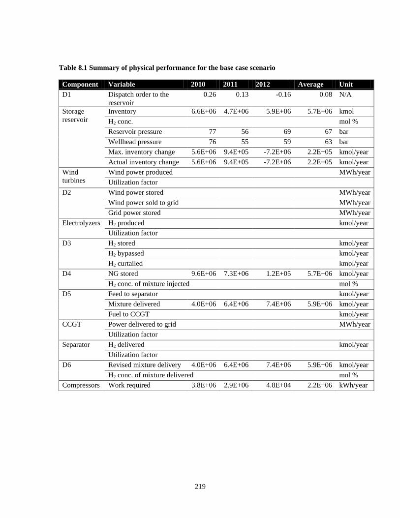
Table 8.1 Summary of physical performance for the base case scenario
Component Variable 2010 2011 2012 Average Unit D1 Dispatch order to the
reservoir 0.26 0.13 -0.16 0.08 N/A
Storage reservoir
Inventory 6.6E+06 4.7E+06 5.9E+06 5.7E+06 kmol H2 conc. mol % Reservoir pressure 77 56 69 67 bar Wellhead pressure 76 55 59 63 bar Max. inventory change 5.6E+06 9.4E+05 -7.2E+06 2.2E+05 kmol/year Actual inventory change 5.6E+06 9.4E+05 -7.2E+06 2.2E+05 kmol/year
Wind turbines
Wind power produced MWh/year Utilization factor
D2 Wind power stored MWh/year Wind power sold to grid MWh/year Grid power stored MWh/year
Electrolyzers H2 produced kmol/year Utilization factor
D3 H2 stored kmol/year H2 bypassed kmol/year H2 curtailed kmol/year
D4 NG stored 9.6E+06 7.3E+06 1.2E+05 5.7E+06 kmol/year H2 conc. of mixture injected mol %
D5 Feed to separator kmol/year Mixture delivered 4.0E+06 6.4E+06 7.4E+06 5.9E+06 kmol/year Fuel to CCGT kmol/year
CCGT Power delivered to grid MWh/year Utilization factor
Separator H2 delivered kmol/year Utilization factor
D6 Revised mixture delivery 4.0E+06 6.4E+06 7.4E+06 5.9E+06 kmol/year H2 conc. of mixture delivered mol %
Compressors Work required 3.8E+06 2.9E+06 4.8E+04 2.2E+06 kWh/year
219
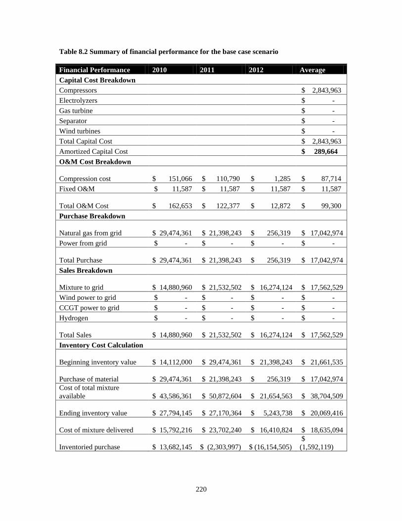
Table 8.2 Summary of financial performance for the base case scenario
Financial Performance 2010 2011 2012 Average Capital Cost Breakdown
Compressors
$ 2,843,963 Electrolyzers
$ -
Gas turbine
$ - Separator
$ -
Wind turbines
$ - Total Capital Cost
$ 2,843,963
Amortized Capital Cost
$ 289,664 O&M Cost Breakdown
Compression cost
$ 151,066 $ 110,790 $ 1,285 $ 87,714
Fixed O&M $ 11,587 $ 11,587 $ 11,587 $ 11,587
Total O&M Cost $ 162,653 $ 122,377 $ 12,872 $ 99,300
Purchase Breakdown
Natural gas from grid $ 29,474,361 $ 21,398,243 $ 256,319 $ 17,042,974
Power from grid $ - $ - $ - $ -
Total Purchase $ 29,474,361 $ 21,398,243 $ 256,319 $ 17,042,974
Sales Breakdown
Mixture to grid $ 14,880,960 $ 21,532,502 $ 16,274,124 $ 17,562,529
Wind power to grid $ - $ - $ - $ - CCGT power to grid $ - $ - $ - $ - Hydrogen $ - $ - $ - $ -
Total Sales $ 14,880,960 $ 21,532,502 $ 16,274,124 $ 17,562,529
Inventory Cost Calculation
Beginning inventory value $ 14,112,000 $ 29,474,361 $ 21,398,243 $ 21,661,535
Purchase of material $ 29,474,361 $ 21,398,243 $ 256,319 $ 17,042,974
Cost of total mixture available
$ 43,586,361 $ 50,872,604 $ 21,654,563 $ 38,704,509
Ending inventory value $ 27,794,145 $ 27,170,364 $ 5,243,738 $ 20,069,416
Cost of mixture delivered $ 15,792,216 $ 23,702,240 $ 16,410,824 $ 18,635,094
Inventoried purchase $ 13,682,145
$ (2,303,997)
$ (16,154,505)
$ (1,592,119)
220

Table 8.3 Net annual cash flow for the base case scenario
Annual Cash Flow 2010 2011 2012 Average 1. Capital costs $ (289,664) $ (289,664) $ (289,664) $ (289,664) 2. OM costs $ (99,300) $ (99,300) $ (99,300) $ (99,300) 3. Cost of sales $ (15,792,216) $ (23,702,240) $ (16,410,824) $ (18,635,094) 4. Sales $ 14,880,960 $ 21,532,502 $ 16,274,124 $ 17,562,529 5. Annual net $ (1,300,221) $ (2,558,703) $ (525,665) $(1,461,529)
Table 8.4 Summary of environmental performance for the base case scenario
Environmental Performance 2010 2011 2012 Average Emission Incurred (kg CO2/year)
Compression of natural gas 2.18E+06 1.67E+06 2.75E+04 1.29E+06 Grid power generation for H2
Mixture use at CCGT Wind power generation for H2
Off-site mixture use 1.76E+08 2.81E+08 3.24E+08 2.60E+08
Emission Mitigated (kg CO2/year) Displacement of SMR H2
Off-site NG use 1.76E+08 2.81E+08 3.24E+08 2.60E+08 NG use at CCGT
Net Emission Calculation (kg CO2/year)
1.29E+06
221

8.2 Mid-Term Scenario: Hydrogen Injection
In this scenario, the operations of the energy hub are identical to those in the base case, with the
exception that hydrogen is being injected into the reservoir during periods of low electricity
prices. Since the dispatch order to the reservoir is the same as the one for the base case scenario,
Figure 2.8 appears to be quasi-identical to Figure 2.2.
Figure 8.7 Dispatch to reservoir for the hydrogen injection scenario
The actual hourly flow rates into and out of the reservoir is the same as the
deliverability/injectability values set by the reservoir model, as specified at decision points D4
and D5 (Figure 2.9).
Q1 2010
-1.0-0.50.00.51.0
-4K
Measure Names
222

Figure 8.8 Injectability/deliverability and actual reservoir flow rates for the hydrogen
injection scenario
The conditions in the reservoir for the hydrogen injection scenario are essentially identical to
those in the base case scenario (compare Figure 2.10 to Figure 2.4). The only significant
difference is that the concentration of hydrogen of the stored gas is now non-zero: the three year
average of the reservoir hydrogen concentration is about 2% (Table 2.5). The hydrogen injected is
produced using grid power, when the market price of electricity is relatively low. The amount of
grid power consumed by the electrolyzer to produce hydrogen is shown in Figure 2.11.
The electrolyzers used for the production of hydrogen show an average utilization factor of ~50%
(Figure 2.12). Over the three years, only 36.5% of the hydrogen produced is stored, the rest needs
to be absorbed by client demand at the time of production (Figure 2.13).
Q1 2010
-4K-2K0K2K4K
-4K
Measure Names
223
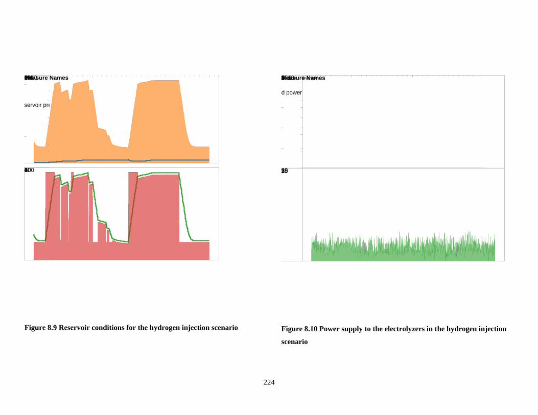
Figure 8.9 Reservoir conditions for the hydrogen injection scenario
Figure 8.10 Power supply to the electrolyzers in the hydrogen injection
scenario
2010
0M2M4M6M8M
0
20406080100
servoir pre
0%
Measure Names
2010
02468
0
510152025
id power
0
Average AverageMeasure Names
224

Figure 8.11 Electrolyzer utilization for the hydrogen injection scenario
Figure 8.12 Outcome of electrolytic hydrogen produced for the hydrogen
injection scenario
2010
050100150200250
0.0
0.20.40.60.81.0
lization fa
2010
0K2K4K
0K
2K4K
stored (km
0K
2K4K
curtailed (
Measure Names
225

The concentration of the mixture stream injected into the reservoir varies widely, from negligible to
100%. Especially high concentrations of hydrogen can occur when the flow rate of natural gas injected is
low (first half of 2012).
Figure 8.13 Flow rates of injected streams for the hydrogen injection scenario
2010
0K1K2K3K4K5K
0.0
Measure Names
226

Figure 8.14 Dispatch of the produced mixture for the hydrogen injection
scenario
Figure 8.15 Value of inventory for the hydrogen injection scenario
Q1 2010
0K2K4K
0K
2K4K
rator feed 0K
2K4K
ure delivere
Measure Names
Q3 2010
0M2M4M6M8M
$0M
Measure Names
227

Table 8.5 Summary of physical performance for the hydrogen injection scenario
Component Variable 2010 2011 2012 Average Unit D1 Dispatch order to the
reservoir 0.26 0.13 -0.16 0.08 N/A
Storage reservoir
Inventory 6.5E+06 4.7E+06 5.9E+06 5.7E+06 kmol H2 conc. 1% 2% 2% 2% mol % Reservoir pressure 77 56 69 67 bar Wellhead pressure 76 55 59 63 bar Max. inventory change 5.6E+06 9.8E+05 -7.2E+06 -2.2E+05 kmol/year Actual inventory change 5.6E+06 9.8E+05 -7.2E+06 -2.2E+05 kmol/year
Wind turbines
Wind power produced MWh/year Utilization factor
D2 Wind power stored MWh/year Wind power sold to grid MWh/year Grid power stored 3.8E+04 3.6E+04 3.9E+04 3.8E+04 MWh/year
Electrolyzers H2 produced 3.5E+05 3.4E+05 3.6E+05 3.5E+05 kmol/year Utilization factor 50% 47% 51% 49%
D3 H2 stored 2.4E+05 1.3E+05 2.0E+04 1.3E+05 kmol/year H2 bypassed 1.2E+05 2.1E+05 3.4E+05 2.2E+05 kmol/year H2 curtailed kmol/year
D4 NG stored 9.3E+06 7.2E+06 3.7E+04 5.5E+06 kmol/year H2 conc. of mixture injected
14% 14% 47% 25% mol %
D5 Feed to separator kmol/year Mixture delivered 4.0E+06 6.3E+06 7.3E+06 5.9E+06 kmol/year Fuel to CCGT kmol/year
CCGT Power delivered to grid MWh/year Utilization factor
Separator H2 delivered kmol/year Utilization factor
D6 Revised mixture delivery 4.0E+06 6.3E+06 7.3E+06 5.9E+06 kmol/year H2 conc. of mixture delivered
1% 2% 2% 2% mol %
Compressors Work required 4.4E+06 3.6E+06 1.0E+06 3.0E+06 kWh/year
228

Table 8.6 Summary of financial performance for the hydrogen injection scenario
Financial Performance 2010 2011 2012 Average Capital Cost Breakdown
Compressors
$ 3,784,995 Electrolyzers
$ 25,463,526
Gas turbine
$ - Separator
$ -
Wind turbines
$ - Total Capital Cost
$ 29,248,521
Amortized Capital Cost
$ 2,979,026
O&M Cost Breakdown Compression cost $ 180,479 $ 141,812 $ 27,898 $ 116,730
Fixed O&M $ 119,161 $ 119,161 $ 119,161 $ 119,161 Total O&M Cost $ 299,640 $ 260,973 $ 147,059 $ 235,891
Purchase Breakdown Natural gas from grid $ 28,530,669 $ 20,984,313 $ 80,742 $ 16,531,908
Power from grid $ 1,121,031 $ 815,788 $ 669,578 $ 868,799 Total Purchase $ 29,651,700 $ 21,800,101 $ 750,320 $ 17,400,707
Sales Breakdown Mixture to grid $ 14,755,856 $ 20,968,870 $ 15,844,113 $ 17,189,613
Wind power to grid $ - $ - $ - $ - CCGT power to grid $ - $ - $ - $ - Hydrogen $ 1,178,990 $ 2,086,901 $ 3,400,559 $ 2,222,150 Total Sales $ 15,934,846 $ 23,055,771 $ 19,244,672 $ 19,411,763
Inventory Cost Calculation Beginning inventory value $ 14,112,000 $ 27,565,298 $ 27,028,642 $ 22,901,980
Purchase of material $ 29,651,700 $ 21,800,101 $ 750,320 $ 17,400,707 Cost of total mixture available $ 43,763,700 $ 49,365,399 $ 27,778,962 $ 40,302,687 Ending inventory value $ 27,565,298 $ 27,028,642 $ 5,234,682 $ 19,942,874 Cost of mixture delivered $ 16,198,402 $ 22,336,757 $ 22,544,280 $ 20,359,813 Inventoried purchase $ 13,453,298 $ (536,656) $ (21,793,960) $ (2,959,106)
229

Table 8.7 Net annual cash flow for the hydrogen injection scenario
Annual Cash Flow 2010 2011 2012 Average 1. Capital costs $ (2,979,026) $ (2,979,026) $ (2,979,026) $ (2,979,026) 2. OM costs $ (235,891) $ (235,891) $ (235,891) $ (235,891) 3. Cost of sales $ (16,198,402) $ (22,336,757) $ (22,544,280) $ (20,359,813) 4. Sales $ 15,934,846 $ 23,055,771 $ 19,244,672 $ 19,411,763 5. Annual net $ (3,478,473) $ (2,495,903) $ (6,514,525) $(4,162,967)
Difference from Base Case ($/year)
$ (2,701,438)
Table 8.8 Summary of environmental performance for the hydrogen injection scenario
Environmental Performance 2010 2011 2012 Average Emission Incurred (kg CO2/year)
Compression of natural gas 2.55E+06 2.10E+06 5.81E+05 1.74E+06 Grid power generation for H2 5.88E+06 3.90E+06 4.18E+06 4.66E+06 Mixture use at CCGT
Wind power generation for H2 Off-site mixture use 1.73E+08 2.71E+08 3.14E+08 2.53E+08
Emission Mitigated (kg CO2/year) Displacement of SMR H2 2.50E+06 4.43E+06 7.22E+06 4.72E+06 Off-site NG use 1.76E+08 2.78E+08 3.20E+08 2.58E+08 NG use at CCGT
Net Emission Calculation (kg CO2/year) -3.41E+06
Difference from Base Case (kg CO2/year) -4.71E+06
230

8.3 Long-Term Scenario: Surplus Baseload Generation (SBG) Reduction
In this scenario, the energy hub is equipped to produce hydrogen for energy storage and to deliver
stored energy to the power grid via the use of an on-site CCGT plant. The dispatch issued to the
reservoir is based on the deviation of Ontario power demand from its annual moving average.
Figure 8.16 Dispatch to reservoir for the SBG reduction scenario
It can be seen that the dispatch order shifts rather violently, from hour to hour, making the figure
indecipherable at hourly resolution. The same information is plotted, averaged by day (i.e. the
dispatch order is averaged for distinct groups of 24 hours) in Figure 2.18. Once averaged by day,
which reduces the visibility of hourly fluctuations, it can be seen that the dispatch order to the
reservoir is largely organized by season. Spring and autumn represent periods of injection (positive
dispatch order); summer and winter represent periods of withdrawal (negative dispatch order).
Q1 2010
-1.0-0.50.00.51.0
-4K
Measure Names
231

Figure 8.17 Daily average of dispatch to reservoir for the SBG reduction scenario
Figure 8.18 Injectability/deliverability and actual reservoir flow rates for the SBG reduction
scenario
Q1 2010
-1.0-0.50.00.51.0
-4K
Measure Names
Q1 2010
-4K-2K0K2K4K
-4K
Measure Names
232

The inventory level for this simulated scenario follows the seasonal pattern dictated by its dispatch
order, with peaks during spring and autumn and troughs during summer and winter. The 3-year
average for hydrogen concentration inside of the reservoir is 1% (Table 2.9). Its profile is relatively
flat, except for the first two months during which hydrogen is initially introduced into the reservoir.
In Figure 2.4, it can be seen that wellhead pressure undergoes many high frequency low-magnitude
changes.
Figure 8.19 Reservoir conditions for the SBG reduction scenario
2010
0M2M4M6M8M
0
20406080100
servoir pre
0%
Measure Names
233
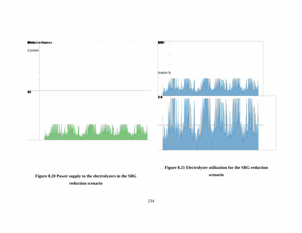
Figure 8.20 Power supply to the electrolyzers in the SBG
reduction scenario
Figure 8.21 Electrolyzer utilization for the SBG reduction
scenario
2010
02468
0
510152025
d power
0
Average AverageMeasure Names
2010
050100150200250
0.0
0.20.40.60.81.0
lization fa
234

From Figure 2.21, a clearly visible seasonal trend can be detected: during periods of low demand, the
electrolyzers operate nearly every hour, consuming a daily average of ~8MW (close to 100%
utilization) , whereas during periods of high electricity demand in Ontario, that value drops to 2-3
MW (about 30% utilization).
Figure 2.23 shows that not all hydrogen produced by the electrolyzers is stored via injection.
Actually, of all the hydrogen produced by the electrolyzer, 60% has been injected into the reservoir.
The rest needed to be absorbed by local hydrogen demand at the time of production (Table 2.9).
Figure 8.22 Outcome of electrolytic hydrogen produced for the SBG reduction scenario
Compared to the hydrogen concentration in the injected mixture for the previous scenario (Figure
2.14), the concentration in this scenario is much more stable, limited to 0% to 30%. The overall
average of hydrogen concentration in the injected stream is 3%.
2010
0K2K4K
0K
2K4K
stored (km
0K
2K4K
curtailed (
Measure Names
235

Figure 8.23 Flow rates of injected streams for the SBG reduction scenario
As expected, the CCGT plant is operated whenever there is production of stored gas from the
reservoir. The quantity of mixture consumed by the on-site CCGT is less than 10% of that delivered
to off-site customers via the distribution pipelines. The utilization of the CCGT plant is about 50%
(Figure 2.26), about the same as the electrolyzers.
2010
0K1K2K3K4K5K
0.0
Measure Names
236
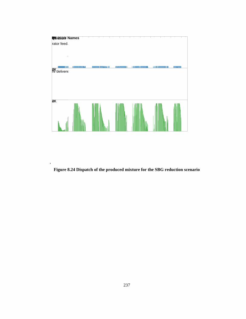
,
Figure 8.24 Dispatch of the produced mixture for the SBG reduction scenario
Q1 2010
0K2K4K
0K
2K4K
arator feed 0K
2K4K
ure delivere
Measure Names
237

Figure 8.25 CCGT utilization for the SBG reduction scenario
Figure 8.26 Value of inventory for the SBG reduction scenario
Q4 2009
010203040
0.0
0.20.40.60.81.0
lization fa
Q3 2010
0M2M4M6M8M
$0M
Measure Names
238

Table 8.9 Summary of physical performance for the SBG reduction scenario
Component Variable 2010 2011 2012 Average Unit D1 Dispatch order to the
reservoir -0.09 0.02 -0.04 -0.03 N/A
Storage reservoir
Inventory 4.4E+06 5.4E+06 5.0E+06 4.9E+06 kmol H2 conc. 1% 1% 1% 1% mol % Reservoir pressure 54 64 60 59 bar Wellhead pressure 53 61 57 57 bar Max. inventory change 1.8E+06 1.2E+06 -1.7E+06 4.6E+05 kmol/year Actual inventory change 1.8E+06 1.2E+06 -1.7E+06 4.6E+05 kmol/year
Wind turbines
Wind power produced MWh/year Utilization factor
D2 Wind power stored MWh/year Wind power sold to grid MWh/year Grid power stored 3.5E+04 3.9E+04 3.7E+04 3.7E+04 MWh/year
Electrolyzers H2 produced 3.2E+05 3.6E+05 3.4E+05 3.4E+05 kmol/year Utilization factor 46% 51% 48% 48%
D3 H2 stored 2.0E+05 2.3E+05 1.9E+05 2.1E+05 kmol/year H2 bypassed 1.3E+05 1.3E+05 1.5E+05 1.4E+05 kmol/year H2 curtailed kmol/year
D4 NG stored 1.5E+07 1.6E+07 1.5E+07 1.5E+07 kmol/year H2 conc. of mixture injected
4% 3% 3% 3% mol %
D5 Feed to separator kmol/year Mixture delivered 1.2E+07 1.4E+07 1.5E+07 1.6E+07 kmol/year Fuel to CCGT 1.5E+06 1.5E+06 1.7E+06 1.6E+06 kmol/year
CCGT Power delivered to grid 1.7E+05 1.7E+05 1.9E+05 1.8E+05 MWh/year Utilization factor 49% 48% 53% 50%
Separator H2 delivered kmol/year Utilization factor
D6 Revised mixture delivery 1.2E+07 1.4E+07 1.5E+07 4.0E+07 kmol/year H2 conc. of mixture delivered
1% 1% 1% 1% mol %
Compressors Work required 5.0E+06 5.7E+06 5.2E+06 1.6E+07 kWh/year
239

Table 8.10 Summary of financial performance for the SBG reduction scenario
Financial Performance 2010 2011 2012 Average Capital Cost Breakdown
Compressors
$ 3,784,995 Electrolyzers
$ 25,463,526
Gas turbine
$ 29,944,756 Separator
$ -
Wind turbines
$ - Total Capital Cost
$ 59,193,277
Amortized Capital Cost
$ 6,028,966
O&M Cost Breakdown Compression cost $ 195,709 $ 226,861 $ 136,056 $ 186,209
Fixed O&M $ 241,159 $ 241,159 $ 241,159 $ 241,159 Total O&M Cost $ 436,868 $ 468,020 $ 377,215 $ 427,368
Purchase Breakdown Natural gas from grid $ 44,473,714 $ 48,802,563 $ 29,725,676 $ 41,000,651
Power from grid $ 1,024,681 $ 959,970 $ 626,722 $ 870,458 Total Purchase $ 45,498,396 $ 49,762,533 $ 30,352,399 $ 41,871,109
Sales Breakdown Mixture to grid $ 38,998,303 $ 41,175,297 $ 33,093,634 $ 37,755,745
Wind power to grid $ - $ - $ - $ - CCGT power to grid $ 6,888,079 $ 5,559,530 $ 4,728,503 $ 5,725,371 Hydrogen $ 1,272,798 $ 1,322,498 $ 1,475,605 $ 1,356,967 Total Sales $ 47,159,179 $ 48,057,326 $ 39,297,742 $ 44,838,082
Inventory Cost Calculation Beginning inventory value $ 14,112,000 $ 12,629,359 $ 15,527,837 $ 14,089,732
Purchase of material $ 45,498,396 $ 49,762,533 $ 30,352,399 $ 41,871,109 Cost of total mixture available $ 59,610,396 $ 62,391,892 $ 45,880,236 $ 55,960,841 Ending inventory value $ 12,629,359 $ 15,527,837 $ 8,609,279 $ 12,255,491 Cost of mixture delivered $ 46,981,037 $ 46,864,055 $ 37,270,957 $ 43,705,350 Inventoried purchase $ (1,482,641) $ 2,898,478 $ (6,918,558) $ (1,834,240)
240
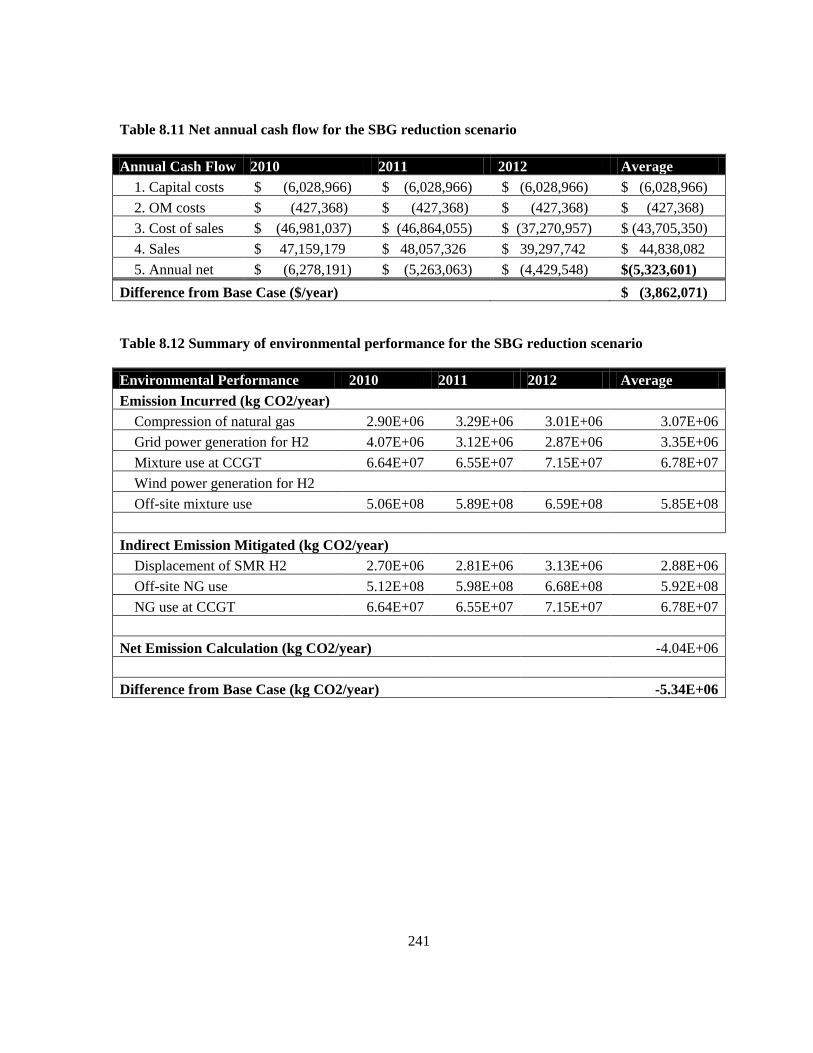
Table 8.11 Net annual cash flow for the SBG reduction scenario
Annual Cash Flow 2010 2011 2012 Average 1. Capital costs $ (6,028,966) $ (6,028,966) $ (6,028,966) $ (6,028,966) 2. OM costs $ (427,368) $ (427,368) $ (427,368) $ (427,368) 3. Cost of sales $ (46,981,037) $ (46,864,055) $ (37,270,957) $ (43,705,350) 4. Sales $ 47,159,179 $ 48,057,326 $ 39,297,742 $ 44,838,082 5. Annual net $ (6,278,191) $ (5,263,063) $ (4,429,548) $(5,323,601)
Difference from Base Case ($/year)
$ (3,862,071)
Table 8.12 Summary of environmental performance for the SBG reduction scenario
Environmental Performance 2010 2011 2012 Average Emission Incurred (kg CO2/year)
Compression of natural gas 2.90E+06 3.29E+06 3.01E+06 3.07E+06 Grid power generation for H2 4.07E+06 3.12E+06 2.87E+06 3.35E+06 Mixture use at CCGT 6.64E+07 6.55E+07 7.15E+07 6.78E+07 Wind power generation for H2
Off-site mixture use 5.06E+08 5.89E+08 6.59E+08 5.85E+08
Indirect Emission Mitigated (kg CO2/year) Displacement of SMR H2 2.70E+06 2.81E+06 3.13E+06 2.88E+06 Off-site NG use 5.12E+08 5.98E+08 6.68E+08 5.92E+08 NG use at CCGT 6.64E+07 6.55E+07 7.15E+07 6.78E+07
Net Emission Calculation (kg CO2/year) -4.04E+06
Difference from Base Case (kg CO2/year) -5.34E+06
241

8.4 Long-Term Scenario: Integration of Wind Power
In this scenario, in additional to the electrolyzer and the CCGT, components which allow for the
storage and recovery of electrical energy via hydrogen, a small scale wind farm is set-up on-site at the
energy hub. The operations of the reservoir, in this case, are directed from the perspective of wind
power generation: wind power generated during off-peak periods is stored for delivery during peak
periods.
From Figure 2.28, it is observed that the dispatch order received by the reservoir is predominantly for
injection (Note that the following figure has been averaged by day to facilitate interpretation).
Figure 8.27 Daily average of dispatch to reservoir for the wind power integration scenario
The injectability/deliverability curve of this scenario displays some unique features. Compared to the
band of dense oscillations which last for most of the simulation, there is a singular increase during the
first few months of storage operation. Also, the maximum deliverability (negative region of the
injectability/deliverability curve) is lower than the maximum injectability.
Q1 2010
-1.0-0.50.00.51.0
-4K
Measure Names
242

Figure 8.28 Injectability/deliverability and actual reservoir flow rates for the wind power
integration scenario
The most striking observation about the reservoir inventory for this scenario is that it does not exhibit
any cycles. In Figure 2.30, the reservoir is shown to be almost always full, except for the first few
months during which it is filled, which is starting with low inventory at the beginning of 2010.
Although the reservoir inventory remains relatively stable for much of the three years under
simulation, the concentration of hydrogen in the reservoir steadily climbs from year to year (2%, 5%
and 6%, respectively).
Q1 2010
-4K-2K0K2K4K
-4K
Measure Names
243

Figure 8.29 Reservoir conditions for the wind power integration scenario
Studying the trend in wellhead pressure in Figure 2.30, it is seen that it is maintained within a very
narrow range: between 103 and 87 bar. Other than that, the wellhead pressure does not exhibit any
clear trend over the time scale chosen. Observing the relationship between the reservoir pressure and
the wellhead pressure over the course of a month, instead of three years, it is observed that the
changes in wellhead pressure are frequent but shallow. Rarely does the wellhead pressure exceed the
reservoir pressure.
2010
0M2M4M6M8M
0
20406080100
servoir pre
0%
Measure Names
244

Figure 8.30 Wellhead pressure and reservoir pressure during March 2010 for the wind power
integration scenario
The overall average capacity utilization factor of wind turbines at the site of the energy hub (Sarnia,
Lambton County, Ontario) is calculated to be 25%, in line with 29.5% the average value for Ontario
wind farms [107]. About 70% of all wind power generated has been used to produce hydrogen; all the
wind power supplied to the electrolyzer, in its turn, represents about 25% of the total electricity
consumption of the electrolyzer, for the time period simulated. The capacity utilization factor of the
electrolyzers is much higher compared to previous scenarios (80% as opposed to 50%) and
experiences no year-to-year variation. More than 75% of the hydrogen produced by the electrolyzer
has been stored.
Mar 4
020406080100
0
Measure Names
245

Figure 8.31 Wind turbines utilization for the wind power integration
scenario
Figure 8.32 Power supply to the electrolyzers in the wind power
integration scenario
2010
0246810
0.0
0.20.40.60.81.0
lization fa
2010
02468
0
510152025
d power
0
Average AverageMeasure Names
246

Figure 8.33 Electrolyzer utilization for the wind power integration
scenario
Figure 8.34 Outcome of electrolytic hydrogen produced for the wind
power integration scenario
2010
050100150200250
0.0
0.20.40.60.81.0
lization fa
2010
0K2K4K
0K
2K4K
stored (km
0K
2K4K
curtailed (
Measure Names
247

Figure 8.35 Flow rates of injected streams for the wind integration
scenario
Figure 8.36 CCGT utilization for the wind power integration scenario
2010
0K1K2K3K4K5K
0.0
Measure Names
Q4 2009
010203040
0.0
0.20.40.60.81.0
lization fa
248

Although the level of the physical inventory of the reservoir seems to stagnate at its maximum
capacity, the value of the gas stored in the reservoir is gradually decreasing.
Figure 8.37 Value of inventory for the wind power integration scenario
Q3 2010
0M2M4M6M8M
$0M
Measure Names
249

Table 8.13 Summary of physical performance for the wind power integration scenario
Component Variable 2010 2011 2012 Average Unit D1 Dispatch order to the
reservoir 0.53 0.53 0.52 0.52 N/A
Storage reservoir
Inventory 8.1E+06 8.4E+06 8.4E+06 8.3E+06 kmol H2 conc. 2% 5% 6% 4% mol % Reservoir pressure 94 99 99 98 bar Wellhead pressure 95 94 94 95 bar Max. inventory change 6.1E+06 -4.5E+04 -7.4E+04 2.0E+06 kmol/year Actual inventory change 6.1E+06 -4.5E+04 -7.4E+04 2.0E+06 kmol/year
Wind turbines
Wind power produced 2.3E+04 2.2E+04 2.2E+04 2.2E+04 MWh/year Utilization factor 26% 25% 25% 25%
D2 Wind power stored 1.5E+04 1.4E+04 1.4E+04 1.4E+04 MWh/year Wind power sold to grid 7.7E+03 7.9E+03 8.1E+03 7.9E+03 MWh/year Grid power stored 4.3E+04 4.4E+04 4.5E+04 4.4E+04 MWh/year
Electrolyzers H2 produced 5.4E+05 5.4E+05 5.4E+05 5.4E+05 kmol/year Utilization factor 76% 76% 76% 76%
D3 H2 stored 4.3E+05 4.1E+05 4.0E+05 4.1E+05 kmol/year H2 bypassed 1.1E+05 1.3E+05 1.4E+05 1.3E+05 kmol/year H2 curtailed kmol/year
D4 NG stored 1.0E+07 5.2E+06 5.6E+06 7.1E+06 kmol/year H2 conc. of mixture injected
14% 17% 16% 16% mol %
D5 Feed to separator kmol/year Mixture delivered 4.0E+06 4.7E+06 5.1E+06 4.6E+06 kmol/year Fuel to CCGT 7.8E+05 9.3E+05 9.9E+05 9.0E+05 kmol/year
CCGT Power delivered to grid 8.7E+04 1.0E+05 1.1E+05 9.9E+04 MWh/year Utilization factor
Separator H2 delivered kmol/year Utilization factor
D6 Revised mixture delivery 4.0E+06 4.7E+06 5.1E+06 4.6E+06 kmol/year H2 conc. of mixture delivered
2% 5% 6% 4% mol %
Compressors Work required 5.0E+06 3.0E+06 3.2E+06 3.8E+06 kWh/year
250

Table 8.14 Summary of financial performance for the wind power integration scenario
Financial Performance 2010 2011 2012 Average Capital Cost Breakdown
Compressors
$ 3,784,995 Electrolyzers
$ 25,463,526
Gas turbine
$ 29,944,756 Separator
$ -
Wind turbines
$ 21,882,706 Total Capital Cost
$ 81,075,983
Amortized Capital Cost
$ 8,257,768
O&M Cost Breakdown Compression cost $ 242,546 $ 121,513 $ 88,609 $ 150,889
Fixed O&M $ 330,311 $ 330,311 $ 330,311 $ 330,311 Total O&M Cost $ 572,857 $ 451,823 $ 418,920 $ 481,200
Purchase Breakdown Natural gas from grid $ 39,546,411 $ 15,765,439 $ 11,703,904 $ 22,338,585
Power from grid $ 1,498,881 $ 1,292,831 $ 997,797 $ 1,263,169 Total Purchase $ 41,045,291 $ 17,058,270 $ 12,701,701 $ 23,601,754
Sales Breakdown Mixture to grid $ 12,339,439 $ 13,846,121 $ 10,202,400 $ 12,129,320
Wind power to grid $ 1,164,431 $ 1,201,745 $ 1,238,542 $ 1,201,573 CCGT power to grid $ 3,566,614 $ 3,501,045 $ 2,795,764 $ 3,287,808 Hydrogen $ 1,111,656 $ 1,316,249 $ 1,406,016 $ 1,277,974 Total Sales $ 18,182,139 $ 19,865,160 $ 15,642,722 $ 17,896,674
Inventory Cost Calculation Beginning inventory value $ 14,112,000 $ 34,175,457 $ 29,491,302 $ 25,926,253
Purchase of material $ 41,045,291 $ 17,058,270 $ 12,701,701 $ 23,601,754 Cost of total mixture available $ 55,157,291 $ 51,233,726 $ 42,193,003 $ 49,528,007 Ending inventory value $ 34,175,457 $ 29,491,302 $ 23,441,869 $ 29,036,209 Cost of mixture delivered $ 20,981,835 $ 21,742,424 $ 18,751,134 $ 20,491,798 Inventoried purchase $ 20,063,457 $ (4,684,154) $ (6,049,433) $ 3,109,956
251

Table 8.15 Net annual cash flow for the wind power integration scenario
Annual Cash Flow 2010 2011 2012 Average 1. Capital costs $ (8,257,768) $ (8,257,768) $ (8,257,768) $ (8,257,768) 2. OM costs $ (481,200) $ (481,200) $ (481,200) $ (481,200) 3. Cost of sales $ (20,981,835) $(21,742,424) $ (18,751,134) $ (20,491,798) 4. Sales $ 18,182,139 $ 19,865,160 $ 15,642,722 $ 17,896,674 5. Annual net $ (11,538,663) $(10,616,233) $ (11,847,380) $ (11,334,092)
Difference from Base Case ($/year)
$ (9,872,563)
Table 8.16 Summary of environmental performance for the wind integration scenario
Environmental Performance 2010 2011 2012 Average Emission Incurred (kg CO2/year)
Compression of natural gas 2.89E+06 1.76E+06 1.86E+06 2.17E+06 Grid power generation for H2 7.07E+06 5.17E+06 5.18E+06 5.81E+06 Mixture use at CCGT 3.34E+07 3.89E+07 4.11E+07 3.78E+07 Wind power generation for H2 4.29E+05 4.20E+05 4.17E+05 4.22E+05 Off-site mixture use 1.70E+08 1.98E+08 2.09E+08 1.92E+08
Indirect Emission Mitigated (kg CO2/year) Displacement of SMR H2 2.36E+06 2.79E+06 2.99E+06 2.71E+06 Off-site NG use 1.74E+08 2.08E+08 2.22E+08 2.01E+08 NG use at CCGT 3.34E+07 3.89E+07 4.11E+07 3.78E+07
Net Emission Calculation (kg CO2/year) -3.28E+06
Difference from Base Case (kg CO2/year) -4.57E+06
252

8.5 Long-Term Scenario: Meeting Large Hydrogen Demand
In this scenario, hydrogen is injected into a natural gas storage reservoir, with a pre-existing amount
of natural gas present as cushion gas. No natural gas is injected into the reservoir with hydrogen, and
the signals on which reservoir operations is based are the schedule of hydrogen demand and the
varying production of hydrogen.
In Figure 2.39 (displaying daily averages), it is seen that the reservoir is subjected to injection most of
the time, given that the dispatch (reservoir mode) is mostly above zero. Consequently, the
injectability/deliverability of the reservoir is also mostly positive, indicative of high injection
potential, but low withdrawal potential.
Figure 8.38 Daily average of dispatch to reservoir for the large hydrogen demand scenario
Because only hydrogen is injected into the reservoir in this scenario, and the scale of hydrogen
production is moderate (26.1 MW or 242 kmol/h), the actual flow rate for injection is much smaller
than the injectability allowed by the reservoir conditions. At the same time, the flow rates withdrawn
from the reservoir is largely limited by the deliverability (Figure 2.40).
Q1 2010
-1.0-0.50.00.51.0
-4K
Measure Names
253

Figure 8.39 Injectability/deliverability and actual reservoir flow rates for the large hydrogen
demand scenario
Compared to the previous scenario, the inventory level in this last scenario is also flat, devoid of
characteristics of storage cycles. But, it remains in the lower end of the spectrum instead (Figure
2.41). Due to the absence of natural gas injection, the concentration of hydrogen in the stored gas
rises much more rapidly than in any of the other scenarios: annual averages are 15%, 38% and 56%,
for 2010-2012 respectively (Table 2.17). In this case, the wellhead pressure appears highly volatile
and does not exhibit any clear trend over the time scale chosen (Figure 2.41).
Q1 2010
-4K-2K0K2K4K
-4K
Measure Names
254

Figure 8.40 Reservoir conditions for the large hydrogen demand
scenario
Figure 8.41 Power supply to the electrolyzers in the large hydrogen
demand scenario
2010
0M2M4M6M8M
0
20406080100
servoir pre
0%
Measure Names
2010
02468
0
510152025
d power
0
Average AverageMeasure Names
255

Figure 8.42 Electrolyzer utilization for the large hydrogen demand
scenario
Figure 8.43 Power supply to the electrolyzers in the large hydrogen
demand scenario
2010
050100150200250
0.0
0.20.40.60.81.0
lization fa
2010
0K2K4K
0K
2K4K
stored (km
0K
2K4K
curtailed (
Measure Names
256
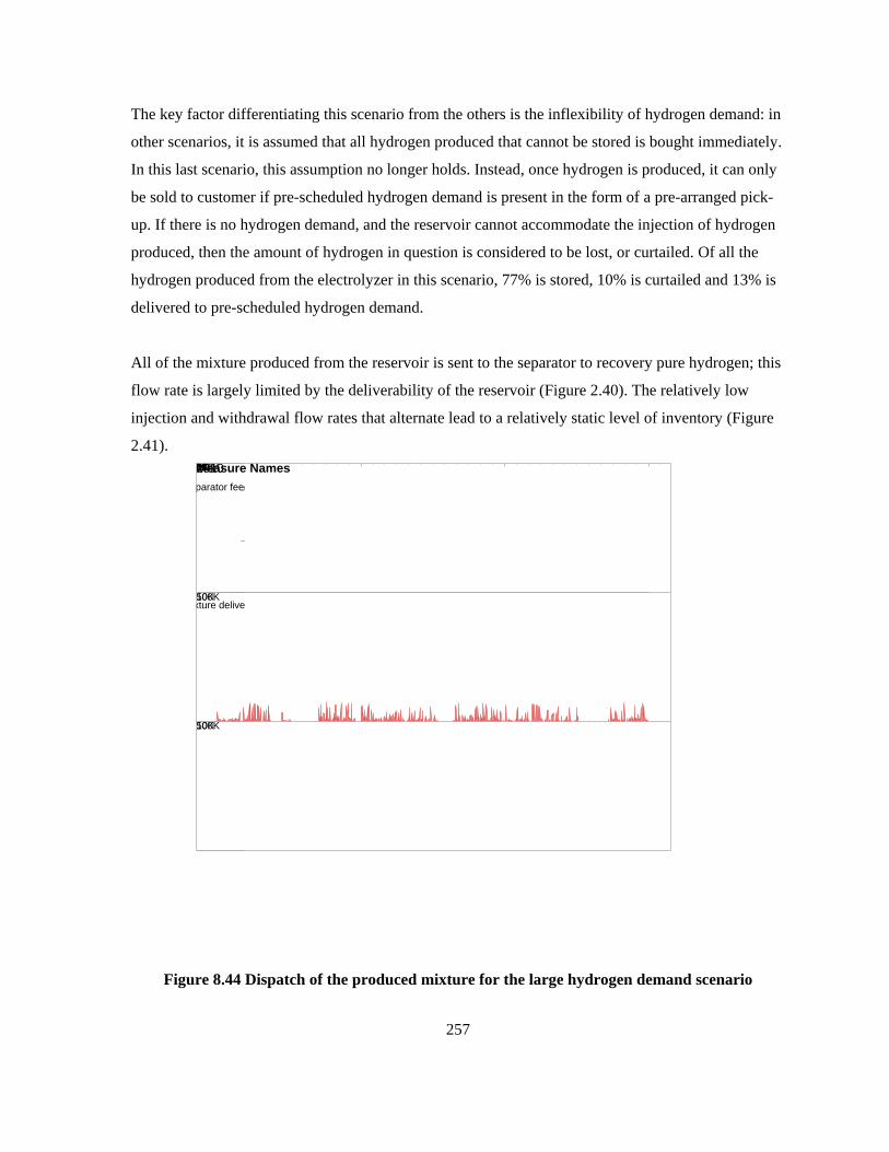
The key factor differentiating this scenario from the others is the inflexibility of hydrogen demand: in
other scenarios, it is assumed that all hydrogen produced that cannot be stored is bought immediately.
In this last scenario, this assumption no longer holds. Instead, once hydrogen is produced, it can only
be sold to customer if pre-scheduled hydrogen demand is present in the form of a pre-arranged pick-
up. If there is no hydrogen demand, and the reservoir cannot accommodate the injection of hydrogen
produced, then the amount of hydrogen in question is considered to be lost, or curtailed. Of all the
hydrogen produced from the electrolyzer in this scenario, 77% is stored, 10% is curtailed and 13% is
delivered to pre-scheduled hydrogen demand.
All of the mixture produced from the reservoir is sent to the separator to recovery pure hydrogen; this
flow rate is largely limited by the deliverability of the reservoir (Figure 2.40). The relatively low
injection and withdrawal flow rates that alternate lead to a relatively static level of inventory (Figure
2.41).
Figure 8.44 Dispatch of the produced mixture for the large hydrogen demand scenario
2010
0K50K100K
0K
50K100K
parator feed
0K
50K100K
xture deliver
Measure Names
257
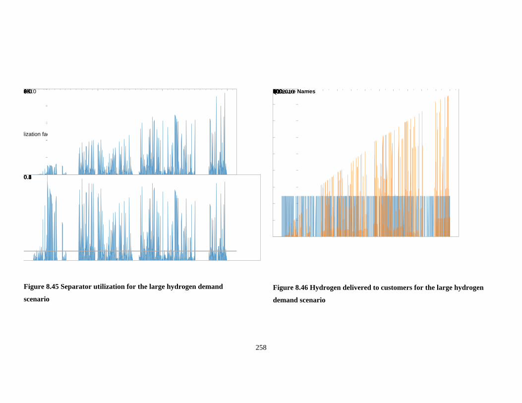
Figure 8.45 Separator utilization for the large hydrogen demand
scenario
Figure 8.46 Hydrogen delivered to customers for the large hydrogen
demand scenario
2010
0K2K4K6K8K
0.0
0.10.20.30.40.5
lization fac
Q3 2010
0100200300400500600700800
0
Measure Names
258

The limited amount of feed dispatched to the separator leads to an especially low capacity utilization
factor: 5% (Figure 2.46). Even during the days with the highest utilization, the daily average capacity
utilization factor does not exceed 50%.
Unlike previous scenarios, in which the hydrogen from bypass is the only source of pure hydrogen,
this last scenario also allows pure hydrogen to be recovered from a natural gas/hydrogen mixture via
the use of the PSA separator. The hourly flow rate of hydrogen that can be recovered through
separation gradually increases, because the feed to the separator is becoming richer in hydrogen
(Figure 2.47). And, the separator is responsible for supplying most of the hydrogen delivered to
customers: about 73%.
Figure 8.47 Hydrogen concentration of mixture delivered for the large hydrogen demand
scenario
2010
0K20K40K60K80K100K120K
0.0
0.20.40.6
servoir H2
0K
Measure Names
259

It is assumed that the natural gas-rich adsorbate from the separator is marketed as hydrogen-enriched
natural gas. Compared to mixture produced directly from storage, the concentration of hydrogen in
this stream has been lowered by undergoing separation of hydrogen from natural gas. When reservoir
concentration of hydrogen has reached 60%, the concentration of the separator “effluent” is about
20% (Figure 2.48).
The gas in storage inside the reservoir experiences a gradual decline in value over the course of three
years. But it occurs at a rate much slower than the decrease in inventory value for the previous
scenarios.
Figure 8.48 Value of inventory for the large hydrogen demand scenario
Q3 2010
0M2M4M6M8M
$0M
Measure Names
260

Table 8.17 Summary of physical performance for the large hydrogen demand scenario
Component Variable 2010 2011 2012 Average Unit D1 Dispatch order to the
reservoir 0.26 0.24 0.27 0.26 N/A
Storage reservoir
Inventory 2.4E+06 2.3E+06 2.3E+06 2.3E+06 kmol H2 conc. 15% 38% 56% 37% mol % Reservoir pressure 32 31 31 31 bar Wellhead pressure 42 35 40 39 bar Max. inventory change 1.8E+07 1.1E+07 1.7E+07 1.5E+07 kmol/year Actual inventory change 1.2E+04 -2.0E+05 1.3E+05 -2.1E+04 kmol/year
Wind turbines
Wind power produced MWh/year Utilization factor
D2 Wind power stored MWh/year Wind power sold to grid MWh/year Grid power stored 1.1E+05 1.1E+05 1.2E+05 1.1E+05 MWh/year
Electrolyzers H2 produced 1.1E+06 1.0E+06 1.1E+06 1.0E+06 kmol/year Utilization factor 50% 47% 51% 49%
D3 H2 stored 8.2E+05 7.0E+05 8.0E+05 7.7E+05 kmol/year H2 bypassed 1.4E+05 1.7E+05 1.9E+05 1.6E+05 kmol/year H2 curtailed 1.0E+05 1.4E+05 9.3E+04 1.1E+05 kmol/year
D4 NG stored kmol/year H2 conc. of mixture injected
100% 100% 100% 100% mol %
D5 Feed to separator 8.1E+05 9.0E+05 6.7E+05 7.9E+05 kmol/year Mixture delivered kmol/year Fuel to CCGT kmol/year
CCGT Power delivered to grid MWh/year Utilization factor
Separator H2 delivered 1.0E+05 2.7E+05 3.0E+05 2.2E+05 kmol/year Utilization factor 5% 6% 5% 5%
D6 Revised mixture delivery 7.1E+05 6.2E+05 3.7E+05 5.7E+05 kmol/year H2 conc. of mixture delivered
4% 11% 20% 12% mol %
Compressors Work required 1.7E+06 2.0E+06 2.3E+06 2.0E+06 kWh/year
261

Table 8.18 Summary of financial performance for the large hydrogen demand scenario
Financial Performance 2010 2011 2012 Average Capital Cost Breakdown
Compressors
$ 5,303,626 Electrolyzers
$ 76,390,578
Gas turbine
$ - Separator
$ 3,453,446
Wind turbines
$ - Total Capital Cost
$ 85,147,649
Amortized Capital Cost
$ 8,672,476
O&M Cost Breakdown Compression cost $ 74,408 $ 80,746 $ 63,555 $ 72,903
Fixed O&M $ 346,899 $ 346,899 $ 346,899 $ 346,899 Total O&M Cost $ 421,307 $ 427,645 $ 410,454 $ 419,802
Purchase Breakdown Natural gas from grid $ - $ - $ - $ -
Power from grid $ 3,363,093 $ 2,447,365 $ 2,008,734 $ 2,606,397 Total Purchase $ 3,363,093 $ 2,447,365 $ 2,008,734 $ 2,606,397
Sales Breakdown Mixture to grid $ 2,159,736 $ 1,763,610 $ 652,935 $ 1,525,427
Wind power to grid $ - $ - $ - $ - CCGT power to grid $ - $ - $ - $ - Hydrogen $ 2,370,634 $ 4,466,426 $ 4,853,506 $ 3,896,856 Total Sales $ 4,530,371 $ 6,230,036 $ 5,506,441 $ 5,422,283
Inventory Cost Calculation Beginning inventory value $ 14,112,000 $ 12,233,591 $ 9,531,972 $ 11,959,188
Purchase of material $ 3,363,093 $ 2,447,365 $ 2,008,734 $ 2,606,397 Cost of total mixture available $ 17,475,093 $ 14,680,956 $11,540,705 $ 14,565,585 Ending inventory value $ 12,233,591 $ 9,531,972 $ 8,282,121 $ 10,015,895 Cost of mixture delivered $ 5,241,502 $ 5,148,985 $ 3,258,584 $ 4,549,690 Inventoried purchase $ (1,878,409) $ (2,701,619) $ (1,249,851) $ (1,943,293)
262

Table 8.19 Net annual cash flow for the large hydrogen demand scenario
Annual Cash Flow 2010 2011 2012 Average 1. Capital costs $ (8,672,476) $ (8,672,476) $ (8,672,476) $ (8,672,476) 2. OM costs $ (419,802) $ - $ - $ (139,934) 3. Cost of sales $ (5,241,502) $ (5,148,985) $ (3,258,584) $ (4,549,690) 4. Sales $ 4,530,371 $ 6,230,036 $ 5,506,441 $ 5,422,283 5. Annual net $ (9,803,409) $ (7,591,425) $ (6,424,619) $ (7,939,818)
Difference from Base Case ($/year)
$ (3,776,851)
Table 8.20 Summary of environmental performance for the large hydrogen demand scenario
Environmental Performance 2010 2011 2012 Average Emission Incurred (kg CO2/year)
Compression of natural gas 9.81E+05 1.18E+06 1.32E+06 1.16E+06 Grid power generation for H2 1.76E+07 1.17E+07 1.25E+07 1.40E+07 Mixture use at CCGT
Wind power generation for H2 Off-site mixture use 3.01E+07 2.45E+07 1.31E+07 2.26E+07
Indirect Emission Mitigated (kg CO2/year) Displacement of SMR H2 5.03E+06 9.48E+06 1.03E+07 8.27E+06 Off-site NG use 3.12E+07 2.75E+07 1.64E+07 2.51E+07 NG use at CCGT
Net Emission Calculation (kg CO2/year) 4.38E+06
Difference from Base Case (kg CO2/year) 3.09E+06
263

8.6 Energy Storage Benchmark Parameters
8.6.1 Roundtrip Efficiency
Because of the definition of the roundtrip efficiency (AC-to-AC), of the three energy storage
pathways – Power to Gas, Power to Power and Power to Hydrogen – only roundtrip efficiency of the
second pathway can be calculated.
Figure 8.49 The Power to Power pathway for the energy hub
Assuming lossless storage, the overall efficiency or the pathway can be calculated as follows:
(1.1)
The rated efficiency of the electrolyzer and the combined cycle gas turbine modeled are 73% and
53% respectively. Therefore, the maximum roundtrip efficiency for the UHNG technology is 39%.
8.6.2 Rated Capacity
The rated storage capacity of the UHNG technology is limited by the storage capacity of the
underground reservoir. Given a specific reservoir pore volume, which is the result of the local
geology, the amount of gas that can be stored varies depending on its temperature, pressure and
264

composition. It can be derived that the rated storage capacity for underground reservoirs is a function
of the reservoir hydrogen concentration.
maxrestotal
res
p VnzRT
= maxrestotal
res
p VnzRT
= (1.2)
2 2, ,H res H res totaln c n= (1.3)
2 2, ,H res HHV H resE E n= (1.4)
2
2
, max,
H res HHV resH res
res
c E p VEz RT
= (1.5)
Given the reservoir parameters in Table 4.5 and a reservoir pressure of 105 bar (maximum limit), the
possible storage capacity using hydrogen storage ranges from 25,000 MWh (2% hydrogen) to
582,000 MWh (100% hydrogen).
Figure 8.50 Rated storage capacity of UHNG as a function of the reservoir hydrogen
concentration
0
100
200
300
400
500
600
700
0% 20% 40% 60% 80% 100%
Rat
ed s
tora
ge c
apac
ity (M
Wh)
Thou
sand
s
Reservoir hydrogen concentration
265

8.6.3 Rated Power
The rated power of the UHNG technology is limited by the component with the lowest power in the
energy storage and recovery pathway. The rated power of the components is first examined.
For the storage reservoir, the maximum rate at which it can store or discharge energy in the form of
hydrogen is limited by its injectability and deliverability. For the reservoir simulated in this project,
the maximum injectability and deliverability are both capped at 5000 kmol/h (Section Injectability
and Deliverability). This molar flow rate is then converted into energy units. Analogous to the storage
capacity, the rated power is also a function of hydrogen concentration of the mixture being stored or
produced. It can vary from 8 MW (2% hydrogen) to 390 MW (100% hydrogen).
2 2,max ,maxH H s HHVP c n E= (1.6)
Figure 8.51 Rated power of reservoir for UHNG as a function of the stored/discharged mixture
hydrogen concentration
For all other components, the rated power of each component is dependent on decisions made by the
energy hub operators with regard to procurement. The rated power of the electrolyzers and the CCGT
0
50
100
150
200
250
300
350
400
450
0% 20% 40% 60% 80% 100%
Rat
ed p
ower
of r
eser
voir
(MW
)
Reservoir hydrogen concentration
266

plant is already known in terms of electrical energy units (MW). However for the CCGT, only the
portion of power that is generated via the combustion of hydrogen is counted; the contribution of the
natural gas present in the mixed fuel is not included:
2 2, , , ,CC H rated H fuel CC ratedW c W= (1.7)
Finally, the rated power of the separator is also found to be a function of the hydrogen concentration
of the feed being processed:
2 2, , , ,H sep rated H feed feed rated sepn c n η= (1.8)
2 2, , , ,sep H rated H sep rated HHVW n E=
(1.9)
( )2 2, , , ,sep H rated H feed feed rated sep HHVW c n Eη=
(1.10)
From the table below, it can be observed that, for all simulation scenarios studied, the reservoir has
always had a rated power that is higher than all other components (8-390MW). In other words, the
rated power of the energy hub, in all scenarios, is limited by the scale of electrolyzers, CCGT or
separator selected, not by the properties of the chosen reservoir. This applies for all scenarios.
Table 8.21Rated power of energy hub components for all scenarios
Scenario Pathway Charging Discharging 1. Base Case N/A 2. Hydrogen Injection Power to Gas Electrolyzers 8.7 MW 3. SBG Reduction Power to Power Electrolyzers 8.7 MW CCGT 0.8-40 MW* 4. Wind Power
Integration Power to Power Electrolyzers 8.7 MW CCGT 0.8-40 MW*
5. Large H2 Demand Power to H2 Electrolyzers 26.1 MW Separator 2- 107 MW* *The range of rated power is determined with hydrogen concentration of 2% and 100%.
267

8.6.4 Self-Discharge rate
In this model of the UHNG technology, it has been assumed that the loss from the storage reservoir is
negligible. However, this may need to be re-evaluated in more detailed models.
A list of potential point of losses has been compiled by Carden and Paterson. They conclude that
once-only losses, associated with the preparation and abandonment of the storage reservoir, are is
more significant than the operating losses (Table 2.22).
The most important once-only loss is the cushion gas that has to remain within the reservoir for the
entire lifetime of the energy storage operations. Other once-only losses are the saturation of connate
water (water trapped inside the pore volume) by the gas in storage and the diffusion of the stored gas
into the ground water surrounding the reservoir. The most important source of operating loss is the
pumping loss, which is, as defined by Carden and Paterson, not a loss of stored material but an energy
loss (i.e. drop in pressure when gas is produced from the reservoir). Given that the storage capacity of
the reservoir selected is 25,000 to 582,000 MWh (variable because of changing hydrogen
concentration); the magnitudes corresponding to the percentages provided can be estimated.
Table 8.22 Summary of sources of losses for underground hydrogen storage [108]
Source % of reservoir capacity Energy loss (MWh)
Cushion gas ~33 8250– 192,000
Solution via connate water ~2 5000 – 116,400
Diffusion ~2 5000 – 116,400
Pumping ~1 per cycle 2500 – 58,200
268

8.6.5 Durability
The durability of the UHNG technology, like its rated power, is dependent on the durability of
individual components. The durability can be either expressed in terms of years (physical lifetime) or
in terms of cycles. Note that only the reservoir is subjected to the storage cycle; all other components
only experience charging or discharging. Therefore, the durability (cycles) measure is not applicable
to them. The durability of the physical reservoir for UHNG is estimated to be of similar scale as that
for CAES, which also involves the use of an underground reservoir.
Table 8.23 Expected lifetime of UHNG technology components [43, 109]
Component Durability (years) Durability (cycles)
Reservoir 20-100 30,000 +
Electrolyzer 5-15 N/A
CCGT 30 N/A
Separator 20+ (columns)
10 (adsorbent)
N/A
8.6.6 Cost of Storage
The cost of storage includes only the capital costs for equipment. The total capital costs is then
normalized using the storage capacity ($/MWh) or the rated power ($/MW). As Table 2.24
demonstrates, the cost of storage is much lower on a capacity basis (less than $4) than on a power
basis (hundreds to tens of thousands of dollars).
269

Table 8.24 Estimated cost of storage for UHNG based on simulation scenarios
Scenario Total Capital Costs ($)
Storage capacity (MWh) Rated Power (MW) Cost
($/kWh) Cost ($/kWh)
Charging Discharging Charging Discharging 1. Base Case 2. Hydrogen Injection 29,248,521 25,000-582,000 8.7 0.05-1.2 3362 3. SBG Reduction 59,193,277 25,000-582,000 8.7 0.8-40 0.10-2.4 6804 1480-73,992 4. Wind Power Integration 81,075,983 25,000-582,000 8.7 0.8-40 0.14-3.2 9319 2027-101,345 5. Large H2 Demand 85,147,649 25,000-582,000 26.1 2-107 0.15-3.4 3262 796-42,574
OVERALL 0.05-3.4 800-74,000
270

Chapter 9 Results Discussion
In this chapter, the results presented in the previous chapter for each of the five scenarios studied are
compared for analysis, so that the impact of various types of decision variables – energy hub
configuration, scale and decision point logic – can be evaluated.
9.1 Base Case Scenario Validation
The base case scenario is the scenario in which the configuration of the energy hub and the scale of
components do not influence the performance indicators. It is used as the baseline for cross-scenario
comparison. Before the comparison of various scenario results, the validity of base case scenario as
modeled is assessed by comparing simulation results from the base case scenario to historical data
available. More specifically, the reservoir inventory for the base case scenario is compared to the
historical inventory level for natural gas storage in Eastern United States (weekly data published by
the EIA, [110]). An energy hub model which has captured the key characteristics of existing UGS
facility operations is expected to generate inventory profile that is similar to the historical one.
Figure 9.1 Comparison of simulated and actual 2010-2012 inventory level for UGS facilities
Q3 2010
0M2M4M6M8M
0
Measure Names
271

Figure 9.1shows that the simulated base case partially conforms to the historical trend of storage
levels. The key similarities and discrepancies are described below:
1. Both set of data exhibit long-term storage cycles: the period for the simulated base case is 7
quarters (21 months), while the period of the historical inventory level is shorter at 4 quarters
(12 months);
2. The rate at which the simulated reservoir is charged and discharged is equal (symmetrical
injectability and deliverability is assumed, reservoir is filled/emptied in the same amount of
time), while the injection rate and withdrawal rate for the historical data set is unequal,
lending to its tilted shape (the charging rate is slower than the discharging rate, the time it
takes to fill the reservoir is longer). Also, at the end of 2012, the injection rate is visibly
different from the two previous years;
3. The inventory of the simulated reservoir always oscillates between the reservoir capacity
maximum and minimum, while the historical inventory shows variable minimum inventory,
i.e. the gas in storage at the end of the heating (producing) season changes from year to year.
It is understood that the key driving force for natural gas storage is the seasonal variation in natural
gas demand. In the base case scenario, at decision point D1, it has been assumed that the price of
natural gas can be used as a proxy indicating the level of demand. Therefore, the market price of
natural gas is used as the main signal that triggers different reservoir operating modes. It is therefore
expected that the reservoir inventory is correlated to the variation in natural gas demand and to the
price of natural gas. This expectation is verified by scatter plots of simulated and historical inventory
levels with respect to demand variation and to price.
The correlation coefficients for the four plots displayed in Figure 9.2 indicate that the historical
inventory level is highly correlated to change in natural gas demand (R = 0.82), whereas the
simulated reservoir inventory is more highly correlated to the price of natural gas (R = 0.45). This
finding suggests that when simulating UGS operations as they have been conducted in the recent past
(2010-2012). A more realistic model logic should be based on the changes in demand for natural gas,
instead of being based on the price of natural gas.
272

Figure 9.2 Correlation of simulated and historical gas storage inventory with respect to A)
natural gas price and B) variation in natural gas demand
Given the constraint for time, the simulated base case is presented and discussed as shown, without
further adjustment of the decision point model logic for better fitting with the historical trend. But, the
discrepancies outlined above are basis over which the model logic for the base case scenario can be
improved upon, for future simulation trials using the same modeling framework.
0
0500100015002000
0M
2M4M6M
servoir inve
R = 0.82
R = 0.22 R = 0.45
R = 0.26
273

9.2 Effect of Decision Variables on Financial Performance Indicators
In this section, the financial performance indicators of all scenarios are compared to the performance
of the base case scenario, and the key differences are explored and discussed. It is important to
remember that, given the limited opportunity for model validation, the comparison presented below is
only meant as sketches of actual possibilities.
9.2.1 Financial Performance Baseline
To begin, it has been found that, the UGS facility at the heart of the UHNG technology, operated as
specified in the base case scenario, leads to an average annual loss of more than $1,400,000. This loss
is mainly caused by the imbalanced cost of sales and revenues from the sales (Figure 9.3). In other
words, the natural gas that is stored, on average, costs more than the price at which they are later sold.
Given that the sales of stored natural gas is the only source of revenue for the base case scenario, it is
impossible to have a positive cash flow, if the revenues from natural gas sales are not enough to cover
the cost of the stored gas.
Figure 9.3 Waterfall chart for the expected annual cash flow of the base case scenario
The cause of this cost imbalance is traced to the overall downward trend in the price of natural gas,
over the period simulated (2010-2012). The profitability of UGS operations is reliant upon the inter-
1. Capital costs
-20M-15M-10M-5M0M($1,461,529)$17,562,529($18,635,094)($99,300)($289,664)
274

seasonal difference in natural gas price, expected because of the seasonal changes in demand. But, as
Figure 9.4 shows, the seasonal term changes expected are suppressed by the larger market force
depressing the price of natural gas over the course of several years, starting from late 2008.
Figure 9.4 Seasonal and annual trend in natural gas price and demand for 2010-2012
The inter-year trend in the price of natural gas is found to be a key factor influencing the operating
profits of UGS facilities. The current approach involves determining project value based on average
annual cash flow from a much shorter simulation period. This rests upon the underlying assumption
that identical cash flow pattern can be expected for all future years of operation. This is an untenable
position if the price of natural gas were to change significantly beyond the period of simulation.
Therefore, when evaluating such a facility over its physical lifetime spanning more than 20 years, it
would be preferable to forecast the long-term price of natural gas over the course of its lifetime, and
to extend the period simulation to be identical to the expected lifetime of the project. For the same
reason, it is decided to not calculate the net present value of the energy hub using the short-term
Q4 2009
0246
0M
1M2M3M
otal gas dema
Minimum Maximum
275

average cash flow, because it is not representative of the long-term average annual cash flow which is
used in NPV calculations.
Figure 9.5 Comparison of financial performance of all scenarios, all values are displayed
relative to the base case value
Compared to the base case scenario, the expected net cash flow of all future scenarios decreased
further (Figure 9.5). Here, all costs items (1,2, and 3) are shown as negative values, so that the annual
net cash flow is the sum of all five items.
Annual Cash FlowScenario11. Capital costs2. OM costs3. Cost of sales4. Sales5. Annual net($8,382,812)
($7,968,104)($5,739,302)($2,689,363)$0
276

Because, other than the change in capital cost, the differences between scenarios are mainly driven by
the changes in the operating profits, the sales and cost of sales are further broken down to be
compared (Figure 9.6).
Figure 9.6 Comparison of operating profits for all scenarios, all values are displayed relative to
the base case value
TypeComponentScenario1Cost of sales
Natural gas from gridPower from gridSalesCCGT power to gridHydrogenMixture to gridWind power to grid($17,042,974)
$5,295,610$23,957,677($511,067)$0
277

Figure 9.7 Shares of purchase by components for all scenarios
Figure 9.8 Shares of sales by components for all scenarios
9.2.2 On Hydrogen Injection
In scenario 2, the additional loss is almost completely attributable to the additional capital cost
requirement: the purchase of the electrolyzer units. There has been a modest increase in operating
profits (Δ Sales +Δ Cost of sales = $124,515), but it barely covers the increase from annual O&M
costs. This increase is mostly from the sales of bypassed hydrogen: the hydrogen that is not stored,
but sold directly to meet local demand.
Because the largest share of revenues for scenario is from the sales of hydrogen-enriched natural gas
(Figure 9.8), the most likely course of action to increase revenues to break even with expenses is to
increase the price of mixture sold. Given that the average amount of mixture delivered per year is 65.9 10× 65.9 10× kmol and the average concentration of hydrogen in the reservoir is 2%
(0.75MMBtu/kmol), the annual output of mixture in terms of energy is 64.4 10× MMBtu (Table 8.5).
Supposing everything else remaining equal (same configuration, scale and decision point logic), to
cover the additional cost incurred by the electrolyzer, the increase in price per MMBtu delivered need
to be $0.60, 16% of the 2010-2012 natural gas price average of $3.77.
Scenario0%
12345Component
Scenario0%
12345Component
278
If the price of mixture delivered cannot be increased, then another option to increase the operating
profit to offset the cost of the electrolyzers is to increase the quantity of hydrogen directly delivered to
meet local demand. However, the assumption that the all hydrogen not stored can be absorbed by
local demand at the moment of its production may no longer hold true as the quantity that needs to be
absorbed increases.
9.2.3 On SBG Reduction
In scenario 3, the volume of sales and its corresponding cost have both increased significantly. This
large change in throughput of the energy storage reservoir is caused by the change in the reservoir
dispatch model logic at decision point D1, reducing the period of a storage cycle from 21 months
(base case) to six months (Figure 8.19), mirroring the peak and off-peak periods for power. This
decrease in periods of storage cycles is also associated with a heightened throughput through the
reservoir. Such a change can be realized practically only if the downstream gas distribution system
can accommodate the increased throughput.
Furthermore, the change in operating profit is positive (Δ Sales +Δ Cost of sales = $2,205,298). It
partially offsets the additional cost of capital (electrolyzers and CCGT), but not completely. The sales
of pure hydrogen and power generated by the on-site CCGT have both contributed to this increase in
operating profit. It is believed that, increasing the utilization factor of the electrolyzer and of the
CCGT should further increase the operating profit. More of the capital cost incurred will be offset, for
the profit margin for hydrogen delivery and power delivery is higher than for mixture delivery
($44/MMBtu H2 and $4.4/MMBtu mixture versus $3.77/MMBtu mixture, respectively). But, the
capacity utilization factors are limited by the decision points specified for this scenario: the
electrolyzers, responsible for producing hydrogen to charge the reservoir, is only run when demand is
low (D2), and, the CCGT, responsible for discharging the reservoir by producing electricity, is only
run when demand is high (D5). It is assumed that the reservoir cannot charge and discharge at the
same time, therefore the utilization factor of each of those components cannot exceed 50%. Unless
the revenues from the sales of hydrogen-enriched natural gas can be increased, an operating loss
seems inevitable because of the high capital cost required by the electrolyzers and the CCGT.
279

At its current scale of energy storage and release, the effect of the energy hub on short-term SGB is
minimal. It is possible for the storage reservoir to accommodate all of the surplus energy available
shown in Figure 9.9 (~370,800 MWh for 10 days), for its rated storage capacity is 25,000 to 582,000
MWh. However, the majority of SBG is available for short periods, with power ranging from
hundreds to thousands of MW. The rate at which energy can be stored delivered by the energy hub
varies between 3-8 MW and 30-40 MW, respectively (Figure 8.20 and Figure 8.25), much too low to
absorb any sizeable portion of the SBG immediately during time of needs.
Figure 9.9 Forecast surplus baseload generation report for July 2013 from the IESO
9.2.4 On Wind Power Integration
In scenario 4 the change in operating profit is negative by much (Δ Sales +Δ Cost of sales = -
$1,552,559), so that the annual loss is even higher than the additional capital investment required. By
examining Figure 9.6, it is found that although the cost of natural gas purchased from the gas grid
increased, the sales of mixture to the grid decreased. This is believed to be caused by the overall
increase in inventory level occurring in this scenario (Figure 8.29), which is in turn cause by the short
duration of the withdrawal window. The FIT schedule with time differentiation as defined by the
Jul 15
0K1K2K3K4K5K6K
50 MW
280

Ontario Power Authority is used as the signal on which reservoir operations are based (D1): the off-
peak hours (128 hours in a week), which incent energy storage, by far outnumber the peak hours (40
hours in a week), which incent energy production.
This scenario is very capital-intensive, since on-site wind turbines are included as part of the energy
hub. It appears that the inclusion of wind turbine did not improve the net cash flow of the energy hub.
Actually, in terms of operating profit, the direct sales of wind power is the most profitable when
compared to all other options: recovering wind power as bypassed hydrogen, recovering wind power
as power generated by the CCGT, or recovering wind power as energy contained in the
hydrogen/natural gas mixture (Table 9.1). Therefore, unless special consideration is given to these
other pathways, for example: special premium prices are provided for hydrogen produced using wind
power or CCGT power partially fuelled by hydrogen produced from wind power, there is no financial
incentive for the energy hub operators to store wind power during off-peak hours. Selling all wind
power disregarding its time of production seems to be the most profitable use of wind turbines.
9.2.5 On Large Hydrogen Demand
In scenario 5, in contrast with scenario 3, in which the volumes of sales and cost of sales both
increased, the two indicators decreased. This is because the scale of injection and withdrawal
occurring is much smaller, since only hydrogen is injected and the mixture is only dispatched to the
separator so that hydrogen can be recovered in its pure form. The resulting change in operating profit
is positive, (Δ Sales +Δ Cost of sales = $1,945,157) mostly from the increased sales of pure hydrogen.
However, this increase is not enough to offset the increase in capital cost required by the electrolyzers
scaled up for this scenario. For this particular scenario, the rated capacity of the electrolyzer has been
increased (26.1 MW as opposed to 8.7 MW for all previous cases), which increased the capital cost
significantly. On the other hand, the separator, although underutilized (Figure 2.45) has relatively low
capital cost (4% of total capital cost).
In three years, the concentration of hydrogen in the reservoir increased steadily to reach 60%. If the
operations were to be maintained, in 2-3 more years, the hydrogen concentration will reach levels
above 90%. As the hydrogen concentration increases, the output of hydrogen by the separator also
281

increases (Figure 8.46). It might be necessary to adjust the mixture withdrawn for separation if the
hydrogen demand cannot accommodate this increase.
282

Table 9.1 Comparison of average profit per energy unit recovered for different storage pathways
Input Value Unit $/unit Conversion required Efficiency Output
Unit $/unit Profit per unit Wind power 1 MWh 0 NO 100% Wind Power 1.00 MWh 115 115.00 Wind power 1 MWh 0 Electrolyzer 70% Bypassed H2 17.77 kg H2 5 88.83 Grid power 1 MWh 30 Electrolyzer 70% Bypassed H2 17.77 kg H2 5 58.83 Grid power 1 MWh 30 Electrolyzer + separator 56% Separated H2 14.21 kg H2 5 41.07 Wind power 1 MWh 0 Electrolyzer + CCGT 35% CCGT Power 0.35 MWh 30 10.50 Wind power 1 MWh 0 Electrolyzer 70% Mixture 2.39 MMBtu 3.7 8.84 Natural gas 1 MMBtu 3.7 CCGT 50% CCGT Power 0.15 MWh 30 0.69 Natural gas 1 MMBtu 3.7 NO 100% Mixture 1.00 MMBtu 3.7 0.00 Grid power 1 MWh 30 Electrolyzer + CCGT 35% CCGT Power 0.35 MWh 30 -19.50 Grid power 1 MWh 30 Electrolyzer 70% Mixture 2.39 MMBtu 3.7 -21.16
Conversion factors: 1 MWh = 3.413 MMBtu, 1 MWh = 25.38 kg H2 (based on HHV), 1 MMBtu = 0.29 MWh
283

9.3 Effect of Decision Variables on Environmental Performance Indicators
Analogous to the financial performance, the emission indicators derived from all five scenarios are
compared, using the base case scenario as the base line.
Given that in the base case, no hydrogen is produced or stored, the so-called mixture produced from
the reservoir is actually pure natural gas. Therefore, it matches the expected emissions from off-site
use of natural gas by end-users. In other words, there is no emission mitigated by using hydrogen-free
natural gas delivered by the energy hub. Then, the net emission from the energy hub is positive and
equivalent to the emissions from compressors used for gas injection.
Figure 9.10 Waterfall chart for the expected annual emission of the base case scenario
The four other scenarios are all compared to the emission profile of the base case, the amount of
emissions incurred by the energy hub and potential emissions mitigated varied widely from one
1. Compression of natural gas
-300M-200M-100M0M100M200M1,292,072-260,212,21400260,212,2140001,292,072
284

scenario to another. However, their relative difference, the net emission, remained relatively constant
for scenarios 2, 3, and 4: net reductions in emission in the order of 5000 tons per year are observed.
Only scenario 5 deviates from this trend: a net increase in of 3000 tons per year is observed (Figure
9.11).
Figure 9.11 Comparison of environmental performance of all scenarios, all values are displayed
relative to the base case value
Although the production and storage of hydrogen reduces potential carbon dioxide emission in most
application scenarios, it is found that when the production of hydrogen becomes important and
consumes a relatively important amount of energy from the grid, there is an increase in net emission.
TypeScenario1Emission Incurre
Emission Mitigate Net Emission Ca
-223,795,885
-23,017,022397,525,760-2,235,7900
285

Given the current supply mix in Ontario, the amount of carbon dioxide emitted by grid-connected
generators exceeds the potential savings from the displacement of hydrogen produced via SMR.
286

Chapter 10 Conclusion
Within the scope of this project, the composite technology of underground storage of hydrogen with
natural gas (UHNG) is proposed and studied using a scenario-based modeling approach. The work
completed to achieve the six research objectives is summarized and presented below. Then, additional
research than can be completed to improve the existing body of work is also suggested.
10.1 Key Decision Variables
Through the formulation of the model of the energy hub, a physical facility embodying the principle
of UHNG, where electric power, natural gas and hydrogen can be conditioned and inter-converted,
three types of key decision variables have been identified:
1. Variables which describe the configuration of energy hub components;
2. Variables which describe the rated capacity of energy hub component; and,
3. Model logics which describe the relationships between exogenous and endogenous process
variables, and the relationship between endogenous process variables.
The first type of variables is binary, indicating the inclusion or exclusion of a given component in the
design of the energy hub. The technological components which can be designated ON/OFF are the
electrolyzers, the CCGT, the separator and the on-site wind turbines. The storage reservoir is a
component by default and should not be excluded. The second type of variables is quantitative,
defining the rated input/output of a given component which is included in the design of the energy
hub. The range of values that these two types of variables can take on can be found in Table 3.1 List
of system configuration and capacity variables.
At six locations within the energy hub model, additional relationships between process variables are
required to completely specify the system of equations that is the model. They are named decision
points and the variables that they need to relate are shown in Table 3.2 List of decision point inputs
and outputs.
287

Other than the three types of decision variables outlined above, another category of variables is found
to exert great influence over the simulation. They are simplified representations of the external
environment with which the energy hub interacts with: the exogenous environmental variables. They
are different from the decision variables in that they cannot be manipulated by the modeler to alter
simulation outcome. Examples include that market price of electricity, the market price of natural gas,
the hourly demand for power in Ontario, etc. The complete list is shown in Table 3.3 List of
exogenous environmental variables.
10.2 Physical Constraints
Three types of constraints have been identified as the most important to model the physical
components of the energy hub: the constraints relating physical output to input, the constraints
limiting the maximum/minimum allowable input or output, and the constraints limiting the difference
between consecutive input/output points. Due to differences in availability of information and level of
complexity, for the six types of components available, the level of detail at which each type of
constraint is captured differs. In the table below, the constraints of every component are briefly
described, and major assumptions or simplifications are stated.
288

Table 10.1 Summary of physical constraints used for component models
Components Constraints on input/output relationship
Constraints on min/max allowable input/output
Constraints on difference in consecutive input/output
Storage reservoir
Basic mass balance and many simplifying assumptions: negligible loss from storage, no water influx, constant volume reservoir, CSTR type mixing.
Calculated assuming that the empirical backpressure equation constants are applicable to production and injection, and that injectability /deliverability is independent of H2 concentration.
Assumed rate of change of wellhead pressure is 1 bar/hour; Assume rate of change of average reservoir pressure (and associated pressure profile) negligible.
Wind turbines
Power curve from manufacturer specifications.
Modular system, rated power depending on number of units.
Estimated to be negligible at hourly timescale.
Electrolyzers Efficiency rating from manufacturer specifications.
Modular system, rated power depending on number of units.
Estimated to be negligible at hourly timescale.
CCGT Calculated from first principles, with some simplification (cold-air standard analysis, 100% combustion efficiency) and use of empirical relationships to relate efficiency of gas turbine cycle to combined cycle efficiency.
Assumed that the same design (same rated efficiency) can be scaled-up or down.
Simplified to be negligible at hourly timescale while it is known that start-up time from standby state requires a few hours.
Separator Assumed based on values from separation experiments/simulations with much higher concentration of H2 in feed.
Range obtained from manufacturer specifications.
Assumed to be negligible at hourly timescale.
Compressors Calculated from first principles + use of empirical efficiency, neglected intercooling required.
No constraint set, units sized based on maximum power requirement.
Estimated to be negligible at hourly timescale.
289

10.3 Benchmark Parameters
The following benchmark parameters have been evaluated based on the physical model established.
They are first estimates which can be used in the comparison of the UHNG concept against other
alternatives for energy storage. The summary of Section 8.6 Energy Storage Benchmark Parameters is
below:
Table 10.2 List of energy storage benchmark parameters for UHNG concept
Parameter Value
Roundtrip efficiency 39%
Rated capacity 25,000 MWh (2% H2) to 582,000 MWh (100% H2), reservoir specific
Rated power* Charging: 8.7-26.1 MW; Discharging: 0.8-107 MW
Self-discharge rate 1% per cycle (energy, not material loss)
Durability 20 years, provided that electrolyzers are replaced
Cost of storage 0.05-3.4 $/kWh; 800-74,000 $/kW
*These values are not the only range of rated power allowed; they are the range of rated power
evaluated in the project, and can be increased/decreased.
10.4 Performance Indicators
Three types of performance indicators have been identified: physical, financial and environmental.
The financial and environmental indicators are derived from the physical performance indicators
available. Therefore, the scope of the physical model and its outputs, the physical performance
indicators, limit the scope of financial and environmental analysis that can be conducted. The most
important physical performance indicators used in this model is the physical inventory of gas in
storage, the concentration of hydrogen in the stored gas, and the flow rate of material/energy stream
from and to the energy hub. For a complete list, please see Table 3.4 List of physical performance
indicators.
The most important financial performance indicators are the capital costs of technological
components included in the energy hub, determined by the configuration and rated input/output of
components, the operating and maintenance costs, the revenues from sales of products delivered by
290

the energy hub, and the cost of the products delivered. The key environmental performance indicators
used are the emissions incurred by the operations of the energy hub and the emissions which have
been displaced by the same operations. For a complete breakdown of components of the financial and
environmental performance model, please refer to Figure 3.17 Scope for financial model and Figure
3.18.
Currently, the simulation is conducted for a period of three years with hourly time step; this departs
from typical timescale of one year. The current timescale is preferred over that of only one year,
because, during preliminary simulation trials, inter-year variations in exogenous environmental
variables, such as the market price of natural gas, are found to have significant influence over the
performance of the energy hub. Therefore, the financial and environmental performance of each of
the three years simulated are compiled and averaged to yield an average annual value used in
reporting. Previously, the determination of the project Net Present Value, an overall financial
performance indicator, was planned; however, since it has been recognized that the inter-year
variability is too great for the extrapolation of life time annual averages (20 years +) from the short-
term simulation results (3 years), the NPV is not calculated.
10.5 Simulation Scenarios
A total of five scenarios have been developed for this simulation study. Each of the scenarios target a
particular use of energy storage through UHNG, with the exception of the base case scenario, in
which a basic UGS facility is simulated, without on-site production and storage of hydrogen. All
scenarios are subjected to the same exogenous environmental variables (market prices of natural gas
and electricity, etc.), but the design and operating philosophy of the energy hub is altered for each
case: a different set of decision variables, judged to be most pertinent to the proposed purpose of the
energy hub, is used as inputs for each scenario. A complete description of the configuration of energy
hub components, rated capacity of components and decision point logic can be found in Chapter 7.
While assembling sets of decision variables for scenarios, it is found that there is most confidence that
the choice of energy hub configuration befits the proposed function (hydrogen injection, SBG
reduction, wind power integration, etc.). The selection of rated capacity for the energy hub
components is based on likelihood of investment: they are sized to be on the small side of the
291

spectrum. It is highly recommended that sensitivity analysis be conducted with respect to the rated
capacity of each energy hub component. Finally, there is a large amount of uncertainty associated
with the choice of model logic at decision points for each scenario. The current choices are at best
educated guesses. In future optimizing studies for the energy hub, the decision points present the most
opportunity for optimization.
10.6 Assessment of Scenarios
Given the uncertainty associated with model components and scenario inputs, as explained by the
sections above, the outputs of the scenario are only meant as sketches and cannot be taken to be exact.
Of all five scenarios, the base case scenario, which only involves basic UGS operations, is the only
one which can be fully compared against actual data for model validation. It is found that existing
natural gas storage practices are more driven by variations in the demand for natural gas than by the
price of natural gas, especially in recent years. If the energy hub were to operate using the decision
point logic as specified by the base case scenario, the energy hub is expected to incur financial losses
for the simulation period chosen. Such losses are mainly caused by the downward trend in market
natural gas prices, which diminish or even eliminate the profitability of temporal arbitrage, the only
source of revenues for the basic UGS facility modeled.
The second scenario involves the injection of hydrogen into the reservoir along with natural gas. Only
one pathway for energy recovery exists for this scenario: the distribution and used of hydrogen-
enriched natural gas by off-site users. This scenario can also be known as the Power to Gas pathway.
It is found that, if operated as the decision points have specified, at the end of three years, the
concentration of hydrogen in the reservoir is expected to increase to 2%. It is not advised to
extrapolate future concentration using the existing simulation results; the preferred course of action is
to extend the simulation for the entire duration of the projects’ lifetime. Then, the long-term hydrogen
concentration can be determined with more certainty. Also, it is found that it is not profitable to sell
the hydrogen-enriched natural gas at the same price as regular natural gas; in order to break even with
the additional costs required by the electrolyzer, a 16% premium is needed for the mixture (basis is
the 2010-2012 average natural gas price of $3.7/MMBtu).
292

The results for the third scenario aimed at reducing Surplus Baseload Generation (SBG) in Ontario is
set up in absence of information of the actual variable level of SBG, the difference between the
hourly Ontario demand and the annual average is used as a proxy signal. It is seen that the estimated
level of SGB shows variation at both short-term and long-term level. Because of the limited rated
input/output of the energy hub compared to its capacity, it is preferable to target long-term trend in
SGB instead of the hourly variations. If hydrogen is still to be stored together with natural gas, then
operating it to store/discharge long-term SGB will alter the pattern of natural gas flow into and out of
the storage reservoir, increasing the throughput of gas through the reservoir and the frequency of
storage cycles.
In the fourth and the last scenario, focused on wind power integration and meeting large supply of
hydrogen, respectively, the level of inventory remained relatively flat throughout the periods of
simulation, without exhibiting clearly visible storage cycles. It is unlikely for the wind power storage
scenario to financially sustainable, if the energy recovered from wind power in the form of hydrogen,
mixture or power is not recognized and given a price different from the market one. As for the large
hydrogen demand scenario, if the energy hub is operated as the scenario specifies, the concentration
of hydrogen inside the reservoir will increase to 60% after three years of storage. The signal used to
trigger energy storage for both scenarios need to be improved. The current signals used to indicate a
need for storage/withdrawal is the time differentiated FIT schedule and a hydrogen pick-up schedule
centered around working hours. Both of them are unbalanced, having more off-peak hours than peak
hours, implying the storage reservoir is more often charged than discharged.
Overall, compared to the base case scenario, the other four scenarios all incurred average annual
losses. In terms of emission, scenario 2, 3, and 4 had limited effect on emission: reductions in the
order of 5000 tons per year are observed. More notable is scenario 5, in which there is relatively
larger scale for production and storage of hydrogen. The emissions incurred by hydrogen production
using grid power actually exceed the potential emissions that can be mitigated through the
corresponding displacement of SMR hydrogen.
293

10.7 Recommendations for Future Research
Given the same modeling frame work, the simulation results that can be obtained will gain in
credibility and accuracy if the following tasks can be carried out:
With respect to exogenous environmental variables used to represent the wider environment in which
the energy hub operates, it would be necessary to extend some of the historical time series currently
used into the future, in order to extend the simulation period to cover the expected physical lifetime of
the project. The exogenous variables that need to be forecasted are: the market price of electricity in
Ontario, the North American market price of natural gas, the demand of electricity in Ontario. To
evaluate the long-term impact of the project, it is preferred to extend the period covered by the
simulation from three historical years (2010-2012) to the actual span of the project’s expected
lifetime (2015 – 2035, possibly). This would require better future projections of natural gas and
electricity pricing, which uses a stochastic approach. The rest of the other exogenous variables need
to be continuously reviewed and replaced better information if available. For example, the market
price for hydrogen-enriched natural gas can be altered to become a function of H2 concentration
instead of being equaled to the price of natural gas), the schedule for hydrogen pick-up at the energy
hub, and the expected level of baseload generators in operation (changes in levels related to
retirement and refurbishment of nuclear power plants).
With respect to physical constraints used in this model, the assumptions and simplifying estimations
listed in Table 10.1 need to be verified experimentally or validated using historical data. Priority is
given to the assumptions associated with the storage reservoir, which is at the heart of the UHNG
concept.
With respect to the performance indicators, it is important to periodically review the indicators chosen
and decide whether additional measures are required to support the decision making process for the
research and development of the UHNG concept. Changes in the performance indicators are likely to
lead to corresponding change in the scope of the physical model. For examples, if local air pollution
is considered to be an important environmental performance indicator, than the current physical
model needs to be modified so that the effect of inputs on local air pollution is captured. A financial
performance indicator omitted from this project is the levelized cost of different energy products
delivered by the energy hub, calculated using accounting cost allocation principles. If included, it 294

should provide more insights on the relative profitability of different energy recovery pathways,
especially when they are available within the same scenario.
With respect to the simulation process itself, it is hoped that sensitivity analysis can be conducted for
the rated capacity of all energy hub components. Following subsequent modeling efforts should make
use of optimization methods to determine the optimal model logic to deploy at the six decision points
identified.
Finally, for this project, the scope of the model, as shown in Figure 3.1 Detailed view of the energy
hub, has been limited to the components contained by the energy hub and simplified representation of
the environment that it interacts with (exogenous environmental variables). This limits the scope of
analysis that can be conducted: all costs and benefits are assessed from the point of the energy storage
facility operator. Therefore, the results from this model are only pertinent to energy storage facility
operators, even when improved along the recommendations given above.
In the case that the performance of UHNG (or any other energy storage technology) needs to be
analyzed from the perspective other than the energy storage facility operators, it is advisable to
gradually expand the scope of model to include other participants in the electricity supply chain. This
is so that system-wide benefits and costs, not directly harvested or born by the operators of energy
storage facilities, can also be assessed. To do this, the elements which have been simplified to be
represented by the exogenous environmental variables (power supply and demand, natural gas supply
and demand, hydrogen supply and demand, etc.) need to be expanded. Their geographic
disaggregation is an essential factor that needs to be explicitly represented in assessing the overall
benefits of storage.
The proposed changes to the scope of the model are illustrated by Figure 10.1. The scope of the
model for this project is approximated by the elements enclosed within Zone C. Elements that are
disaggregated components of the power grid are coloured in yellow; elements which are part of the
disaggregated natural gas grid are coloured in red. The physical constraints of the network lines
connecting the various zones are an integral part of the new model. Using input-output relationships
from the existing modeling framework, a surrogate model can be developed to represent the energy
hub in this expanded study.
295

To understand the full impact of energy storage and whether it should be implemented, it is necessary
to assess the economic costs and benefits from the perspective of the whole system (zone A, B, C and
D, altogether); to understand how individual participant (Baseload generator, NG supplier, NG
consumers, power consumers, etc.) would gain or lose from energy storage and how it can be
implemented, it is necessary to analyze the financial costs and benefits from the perspective of each
participant. The two perspectives complement each other. A system wide simulation with multiple
nodes producing hydrogen, then the nodes injecting and withdrawing mixed natural gas and hydrogen
at different times of the day and year needs to be conducted.
296

Figure 10.1 Expanded scope for future models assessing the benefits of energy storage via the
energy hub
297

References
1. Baxter, R., Energy Storage: a Nontechnical Guide. 2006: PennWell Books. 2. IESO. Composition of Ontario's Electricity Mix Continues to Change: Consumer Response
Supports Reliability. 2012 [cited 2012 August 8th]; Available from: http://www.ieso.ca/imoweb/media/md_newsitem.asp?newsID=5930.
3. IESO, Surplus Baseload Generation (SBG). 2012, IESO. 4. IESO, Forecast Weekly Minimum Demand and Baseload Generation,
18MonthOutlookTables_2013may, Editor. 2013. 5. Ontario Ministry of Energy, Ontario's Feed-in Tariff Program Two-Year Review Report.
2012, Ontario Ministry of Energy: Toronto. 6. Ribeiro, P.F., et al., Energy storage systems for advanced power applications. Proceedings of
the IEEE, 2001. 89(12): p. 1744-1756. 7. Schaber, C., P. Mazza, and R. Hammerschlag, Utility-Scale Storage of Renewable Energy.
The Electricity Journal, 2004. 17(6): p. 21-29. 8. Hadjipaschalis, I., A. Poullikkas, and V. Efthimiou, Overview of current and future energy
storage technologies for electric power applications. Renewable and Sustainable Energy Reviews, 2008. 13(6-7): p. 1513-1522.
9. Oudalov, A., T. Buehler, and D. Chartouni. Utility Scale Applications of Energy Storage. in Energy 2030 Conference, 2008. ENERGY 2008. IEEE. 2008.
10. Electric Power Research Institute, Electricity Energy Storage Technology Options. 2010, Electric Power Research Institute: Palo Alto, CA.
11. Vazquez, S., et al., Energy Storage Systems for Transport and Grid Applications. Industrial Electronics, IEEE Transactions on, 2010. 57(12): p. 3881-3895.
12. International Energy Agency, 2011 Key World Energy Statistics. 2011, International Energy Agency, .
13. Cullen, J.M., Allwood, Julian M., The efficient use of energy: Tracing the global flow of energy from fuel to service. Energy Policy, 2010. 38(1).
14. IESO, Historical Market Data, IESO, Editor. 2012, IESO: Toronto. 15. Duguid, B., Supply Mix Directive, Ministry of Energy, Editor. 2011, Ontario Power
Authority: Canada. 16. Sioshansi, R., Some Policy and Research Questions Related to Energy Storage, in EUI
Working Papers, E.U. Institute, Editor. 2010, Robert Schuman Centre for Advanced Studies: Fiesole, Italy.
17. Sovacool, B.K. and R.F. Hirsh, Beyond batteries: An examination of the benefits and barriers to plug-in hybrid electric vehicles (PHEVs) and a vehicle-to-grid (V2G) transition. Energy Policy, 2009. 37(3): p. 1095-1103.
18. Ibrahim, H., A. Ilinca, and J. Perron, Energy storage systems—Characteristics and comparisons. Renewable and Sustainable Energy Reviews, 2008. 12(5): p. 1221-1250.
19. Divya, K.C. and J. Østergaard, Battery energy storage technology for power systems—An overview. Electric Power Systems Research, 2009. 79(4): p. 511-520.
20. Nomura, S., et al., Technical and Cost Evaluation on SMES for Electric Power Compensation. Applied Superconductivity, IEEE Transactions on, 2010. 20(3): p. 1373-1378.
298

21. Nielsen, L. and R. Leithner, Dynamic Simulation of an Innovative Compressed Air Energy Storage Plant - Detailed Modelling of the Storage Cavern. WSEA Transactions on Power Systems, 2009. 4(8): p. 253-263.
22. IESO. Supply Overview. 2012 [cited 2012 August 8th]; Available from: http://www.ieso.ca/imoweb/media/md_supply.asp.
23. Reuters. Ontario to shut Pickering B nuclear plant in 2020. 2010 [cited 2013 July 19th]; Available from: http://ca.reuters.com/article/domesticNews/idCATRE61F5SP20100216.
24. Krause, T., et al., Multiple-Energy Carriers: Modeling of Production, Delivery, and Consumption. Proceedings of the IEEE, 2011. 99(1): p. 15-27.
25. Geidl, M., Integrated Modeling and Optimization of Multi-Carrier Energy Systems. 2007, ETH Zurich: Zurich.
26. Geidl, M. and G. Andersson, Optimal Power Flow of Multiple Energy Carriers. Power Systems, IEEE Transactions on, 2007. 22(1): p. 145-155.
27. Geidl, M. and G. Andersson. Optimal coupling of energy infrastructures. in PowerTech Conference. 2007. Lausanne, Switzerland.
28. Geidl, M. and G. Andersson. A Modeling and optimization approach for multiple energy carrier power flow. in IEEE PES PowerTech. 2005. St. Petersburg, Russia.
29. Koeppel, G., Reliability considerations of future energy systems: Multi-carrier systems and the effect of energy storage. 2007, Swiss Federal Institute of Technology Zurich: Zurich, Switzerland.
30. Koeppel, G. and G. Andersson. The influence of combined power, gas, and thermal networks on the reliability of supply. in 6th International World Energy System Conference. 2006. Torino, Italy.
31. Koeppel, G. and G. Andersson, Reliability modeling of multi-carrier energy systems. Energy, 2009. 34(3): p. 235-244.
32. Arnold, M., et al. Distributed control applied to combined electricity and natural gas infrastructures. in International Conference on Infastructure Systems and Services. 2008. Rotterdam, The Netherlands.
33. Arnold, M., et al. Model-based predictive control applied to multi-carrier energy systems. in IEEE Power ENergy Society General Meeting. 2009. Calgary, Canada.
34. Kienzle, F., et al., Valuing Investments in Multi-Energy Conversion, Storage, and Demand-Side Management Systems Under Uncertainty. Sustainable Energy, IEEE Transactions on, 2011. 2(2): p. 194-202.
35. Kienzle, F. and G. Andersson, Valuing investments in multienergy generation plants under uncertainty: A real options analysis, in IAEE European Conference. 2009: Vienna.
36. Kienzle, F. and G. Andersson. Location-dependent valuation of energy hubs with storage in multi-carrier energy systems. in Energy Market (EEM), 2010 7th International Conference on the European. 2010.
37. Kienzle, F. and G. Andersson. Efficient multi-energy generation portfolios for the future. in 4th Annual Carnegie Mellon Conference on Electricity Industry. 2008. Pittsburgh, PA.
38. Kienzle, F. and G. Andersson. Comprehensive performance and incertitude analysis of multi-energy portfolio. in IEEE PowerTech. 2009. Bucharest, Romania.
39. Kienzle, F. and G. Andersson. A greenfield approach to the future supply of multiple energy carriers. in Power & Energy Society General Meeting, 2009. PES '09. IEEE. 2009.
40. Cumalioglu, I., et al., State of the Art: Hydrogen storage. Journal of Fuel Cell Science and Technology, 2008. 5(3): p. 034001-10.
41. Holladay, J.D., et al., An overview of hydrogen production technologies. Catalysis Today, 2009. 139(4): p. 244-260.
299

42. Schmid, R. Electrolysis for grid balancing. in International Water Electrolysis Symposium. 2012. Copenhagen, Denmark.
43. Ivy, J., Summary of Electrolytic Hydrogen Production. 2004, National Renewable Energy Laboratory: Golden, Colorado.
44. International Energy Agency, Hydrogen Production and Storage. 2006, International Energy Agency,: Paris.
45. Briguglio, N., et al., Development of a Compact PEM Electrolyzer System for Applications with Microdistributed Renewable Sources. ECS Transactions, 2012. 42(1): p. 95-100.
46. Turner, J.A., Sustainable Hydrogen Production. Science, 2004. 305(5686): p. 972-974. 47. León, A., Hydrogen technology: mobile and portable applications. 2008, Berlin: Springer. 48. International Gas Union. 2006-2009 Triennium Work Report Working Committee 2: Storage.
2009 [cited 2011 December 15th]; SG 2.1 UGS Database]. Available from: http://www.igu.org/html/wgc2009/committee/WOC2/WOC2.pdf.
49. Foh, S., et al., Underground Hydrogen Storage Final Report. 1979, Institute of Gas Technology: Chicago.
50. Katz, D.L. and M.R. Tek, Overview on Underground Storage of Natural Gas. Journal of Petroleum Technology, 1981. 33(6).
51. Plaat, H., Underground gas storage: Why and how. Geological Society, London, Special Publications, 2009. 313(1): p. 25-37.
52. Bary, A., et al., Storing Natural Gas Underground, in Oilfield Reviews. 2002, Schlumberger. 53. Miyazaki, B., Well integrity: An overlooked source of risk and liability for underground
natural gas storage. Lessons learned from incidents in the USA, in Underground Gas Storage: Worldwide Experiences and Future Development in the UK and Europe, E.J. Evans and R.A. Chadwick, Editors. 2009, The Geological Society: London.
54. Laier, T. and H. Øbro, Environmental and safety monitoring of the natural gas underground storage at Stenlille, Denmark, in Underground Gas Storage: Worldwide Experiences and Future Development in the UK and Europe
E.J. Evans and R.A. Chadwick, Editors. 2009: London. 55. Ontario Petroleum Institute. Industry Fast Facts: Ontario. 2003 [cited 2012 July 17th];
Available from: http://www.ontpet.com/documents/ont_fast_facts.pdf. 56. Breeze, P., Gas Turbines and Combined Cycle Power Plants, in Power Generation
Technologies. 2005, Elsevier. 57. Molière, M., Stationary gas turbines and primary energies: A review of fuel influence on
energy and combustion performances. International Journal of Thermal Sciences, 2000. 39(2): p. 141-172.
58. Kehlhofer, R., et al., Combined-Cycle Gas and Steam Turbine Power Plants (3rd Edition). 2009: PennWell.
59. Haeseldonckx, D. and W. D’haeseleer, The use of the natural-gas pipeline infrastructure for hydrogen transport in a changing market structure. International Journal of Hydrogen Energy, 2007. 32(10–11): p. 1381-1386.
60. De Simio, L.G., M; Iannaccone, S. Use of Hydrogen-Methane Mixtures for Heavy Duty Engines. in 12th World IANGV Conference and Exhibition. 2010. Rome.
61. Rahm, S.G., Jeffery; Molière, Michel; Eranki, Aditya, Addressing Gas Turbine Fuel Flexibility, G. Energy, Editor. 2009.
62. Barnicki, S.D. and J.R. Fair, Separation system synthesis: a knowledge-based approach. 2. Gas/vapor mixtures. Industrial & Engineering Chemistry Research, 1992. 31(7): p. 1679-1694.
300

63. Peramanu, S., B.G. Cox, and B.B. Pruden, Economics of hydrogen recovery processes for the purification of hydroprocessor purge and off-gases. International Journal of Hydrogen Energy, 1999. 24(5): p. 405-424.
64. Agarwal, A., Advanced Strategies for Optimal Design and Operation of Pressure Swing Adsorption Processes, in Chemical Engineering. 2010, Carnegie Mellon University: Pittsburgh.
65. NaturalHy, Using the Existing Natural Gas System for Hydrogen. 2009, European Commission's Sixth Framework Programme.
66. National Grid, A.H.I., Hydrogen-Enriched Natural Gas, in World Energy Council. 2009. 67. Clarke, J., Correspondence with senior geologist from Union Gas, Dan Peng, Editor. 2012. 68. Hydrogenics, Technical Specifications for HySTAT-60 Fueling Station. 2011. 69. Vestas, V90-1.8/2.0 MW Maximum output at medium-wind and low-wind sites. 2009. 70. The Linde Group, Hydrogen Recovery by Pressure Swing Adsorption. 2012. 71. Ontario Power Authority. FIT Program Pricing > FIT Price Schedule. 2011 [cited 2011
December 2nd]; Available from: http://fit.powerauthority.on.ca/fit-price-schedule. 72. Energy Information Administration, Henry Hub Gulf Coast Natural Gas Spot Price. 2013,
U.S. Energy Information Administration. 73. Hajimiragha, A., M.W. Fowler, and C.A. Cañizares, Hydrogen economy transition in Ontario
– Canada considering the electricity grid constraints. International Journal of Hydrogen Energy, 2009. 34(13): p. 5275-5293.
74. Canadian Centre for Energy Information. Energy Facts & Statistics - Ontario. [Webpage Table] 2011 2009 December 30th [cited 2011 December 20th]; Available from: http://www.centreforenergy.com/FactsStats/Statistics.asp?Template=5,5.
75. Ontario Energy Board, Natural Gas Regulation in Ontario: A Renewed Policy Framework, in Natural Gas Forum. 2005.
76. Natural Resources Canada, The Atlas of Canada > Pipeline Infrastructure Map. 2009. 77. Statistics Canada, Sales of Natural Gas, Statistics Canada, Editor. 2013. 78. Sustainable Development Technology Canada, Renewable Fuel -- Hydrogen, SD Business
Case. 2006. 79. Cicha, W.V.G., Alan. Hydrogen Production Trends, Canadian Prospects within a Global
Perspective. in World Hydrogen Energy Conference 2012. 2012. Toronto, Canada. 80. Horngren, C.T.D., Srikant M.; Rajan, Madhav, Cost accounting : a managerial emphasis
14th ed. 2012, Upper Saddle River, New Jersey: Pearson. 81. Lemus, R.G. and J.M. Martínez Duart, Updated hydrogen production costs and parities for
conventional and renewable technologies. International Journal of Hydrogen Energy, 2010. 35(9): p. 3929-3936.
82. Read, C.J., DOE Hydrogen Program Overview. 2008, International Energy Agency Hydrogen Implementing Agreement.
83. Ikoku, C.U., Natural Gas Engineering: A system Approach. 1980, Tulsa: PennWell Books. 788.
84. Enbridge. Components of Natural Gas. 2011 [cited 2012 April 11th]; Available from: https://www.enbridgegas.com/gas-safety/about-natural-gas/components-natural-gas.aspx.
85. Hagoort, J., Fundamentals of Gas Reservoir Engineering. Developments in Petroleum Science. 1988, Amsterdam: Elsevier.
86. Flanigan, O., Underground Gas Storage Facilities: Design and Implementation. 1995, Houston: Gulf Professional Publishing.
301

87. Environment Canada. National Climate Data and Information Archive. 2011 May 14th 2013 [cited 2013 May 15th]; Available from: http://www.climate.weatheroffice.gc.ca/climateData/canada_e.html.
88. Cargnelli, J., Bridging Power and Gas Grids. 2011, International Partnership for Hydrogen and Fuel Cells in the Economy.
89. Gandía, L.M., et al., Renewable Hydrogen Production: Performance of an Alkaline Water Electrolyzer Working under Emulated Wind Conditions. Energy & Fuels, 2007. 21(3): p. 1699-1706.
90. Bruynooghe, C., A. Eriksson, and G. Fulli, Load-following operating mode at Nuclear Power Plants and incidence on Operation and Maintenance costs. 2010, European Commission Joint Research Centre.
91. Moran, M.J.S., Howard N., Fundamentals of engineering thermodynamics. 2004, Hoboken: Wiley.
92. Sircar, S. and T.C. Golden, Purification of Hydrogen by Pressure Swing Adsorption. Separation Science and Technology, 2000. 35(5): p. 667-687.
93. Yang, R.T. and S.J. Doong, Gas Separation by Pressure Swing Adsorption: A Pore-Diffusion Model for Bulk Separation. AICHE Journal, 1985. 31(11).
94. Waldron, W.E. and S. Sircar, Parametric Study of a Pressure Swing Adsorption Process. Adsorption, 2000. 6(2): p. 179-188.
95. Brown, R.N., Compressors: Selection and Sizing. 1997: Elsevier Gulf. 96. Walas, S.M., Chemical Process Equipment - Selection and Design. 1990, Elsevier. 97. Weil, S., Hydrogen Delivery: Session Introduction. 2012, U.S. Department of Energy. 98. International Renewable Energy Agency, Wind Power, in Renewable Energy Technologies:
Cost Analysis Series. 2012, International Renewable Energy Agency 99. Prince-Richard, S., A Techno-Economic Analysis of Decentralized Electrolytic Hydrogen
Production fo Fuel Cell Vehicles, in Mechanical Engineering. 2004, University of Victoria: Victoria.
100. Hammerli, M., When will electrolytic hydrogen become competitive? International Journal of Hydrogen Energy, 1984. 9(1–2): p. 25-51.
101. Stucki, S., The cost of electrolytic hydrogen from off-peak power. International Journal of Hydrogen Energy, 1991. 16(7): p. 461-467.
102. Agrawal, R., L. Biegler, and A. Westerberg. Pressure Swing Adsorption Sizing/Costing. Introduction to Air Separation 1999 [cited 2013 April 1st]; a Process Design Case Study
distributed by CACHE Corporation]. Available from: http://www.cheme.cmu.edu/course/06302/airsep2/PSADesign.html.
103. McCollum, D.O., J, Techno-Economic Models for Carbon Dioxide Compression, Transport, and Storage & Correlations for Estimating Carbon Dioxide Density and Viscosity. 2006, Institute of Transporatation Studies UC Davis.
104. Amos, W.A., Costs of Storing and Transporting Hydrogen. 1998, National Renewable Energy Laboratory: Golden, Colorado.
105. Spath, P.L. and M.K. Mann, Life Cycle Assessment of Hydrogen Production via Natural Gas Steam Reforming. 2001, National Renewable Energy Laboratory: Golden.
106. Weisser, D., A guide to life-cycle greenhouse gas (GHG) emissions from electric supply technologies. Energy, 2007. 32(9): p. 1543-1559.
107. Dewees, D.N., The Economics of Renewable Electricity Policy in Ontario. 2013, University of Toronto.
302

108. Carden, P.O. and L. Paterson, Physical, chemical and energy aspects of underground hydrogen storage. International Journal of Hydrogen Energy, 1979. 4(6): p. 559-569.
109. Spath, P.L. and M.K. Mann, Life Cycle Assessment of a Natural Gas Combined-Cycle Power Generation System. 2000, National Renewable Energy Laboratory.
110. Energy Information Administration, Weekly Natural Gas Storage Report, Energy Information Administration, Editor. 2011, Energy Information Administration,
.
303