enabling safe autonomous driving in real-world city traffic using multiple criteria decision making

1939-1390/11/$26.00©2011IEEE

Andrei Furda and Ljubo VlacicIntelligent Control Systems Laboratory (ICSL),

Institute of Integrated and Intelligent Systems, Griffith University, Brisbane, QLD 4111, Australia, E-mails: [email protected]

and [email protected]

IEEE INTELLIGENT TRANSPORTATION SYSTEMS MAGAZINE • 4 • SPRING 2011

Enabling Safe Autonomous Driving in Real-World City

Traffic Using Multiple Criteria Decision Making

© STOCKBYTE

I. Introductionutonomous city vehicles capable of driving safely through urban traffic and shar-ing the roads with other traffic partici-pants, have been a vision for many years

(Kolodko and Vlacic, 2003; Li and Tang, 2009). One of the research topics which are cru-

cial for enabling autonomous vehicles to cope with urban traffic conditions is their ability to make safe and appropriate driving decisions in any traffic situation.

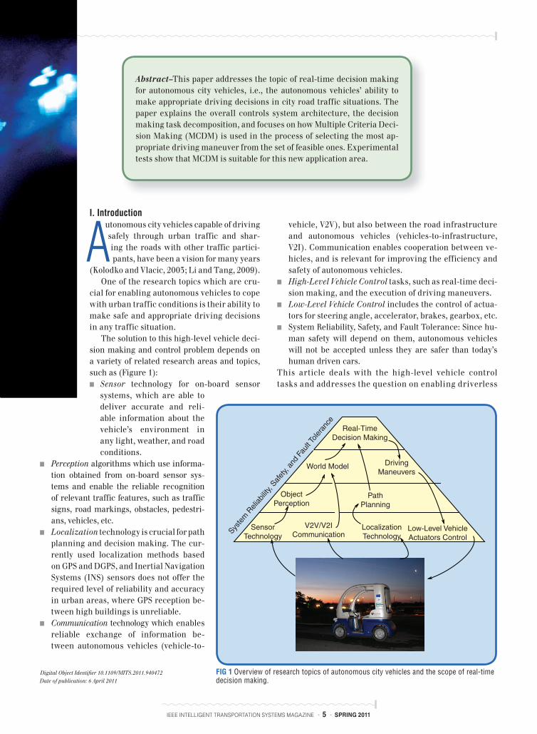
The solution to this high-level vehicle deci-sion making and control problem depends on a variety of related research areas and topics, such as (Figure 1): ■ Sensor technology for on-board sensor

systems, which are able to deliver accurate and reli-able information about the vehicle’s environment in any light, weather, and road conditions.

■ Perception algorithms which use informa-tion obtained from on-board sensor sys-tems and enable the reliable recognition of relevant traffic features, such as traffic signs, road markings, obstacles, pedestri-ans, vehicles, etc.

■ Localization technology is crucial for path planning and decision making. The cur-rently used localization methods based on GPS and DGPS, and Inertial Navigation Systems (INS) sensors does not offer the required level of reliability and accuracy in urban areas, where GPS reception be-tween high buildings is unreliable.

■ Communication technology which enables reliable exchange of information be-tween autonomous vehicles (vehicle-to-

vehicle, V2V), but also between the road infrastructure and autonomous vehicles (vehicles-to-infrastructure, V2I). Communication enables cooperation between ve-hicles, and is relevant for improving the efficiency and safety of autonomous vehicles.

■ High-Level Vehicle Control tasks, such as real-time deci-sion making, and the execution of driving maneuvers.

■ Low-Level Vehicle Control includes the control of actua-tors for steering angle, accelerator, brakes, gearbox, etc.

■ System Reliability, Safety, and Fault Tolerance: Since hu-man safety will depend on them, autonomous vehicles will not be accepted unless they are safer than today’s human driven cars.

This article deals with the high-level vehicle control tasks and addresses the question on enabling driverless


Digital Object Identifier 10.1109/MITS.2011.940472Date of publication: 6 April 2011

Abstract–This paper addresses the topic of real-time decision making for autonomous city vehicles, i.e., the autonomous vehicles’ ability to make appropriate driving decisions in city road traffic situations. The paper explains the overall controls system architecture, the decision making task decomposition, and focuses on how Multiple Criteria Deci-sion Making (MCDM) is used in the process of selecting the most ap-propriate driving maneuver from the set of feasible ones. Experimental tests show that MCDM is suitable for this new application area.

Low-Level VehicleActuators Control

LocalizationTechnology

V2V/V2ICommunication

SensorTechnology

PathPlanning

ObjectPerception

DrivingManeuvers

World Model

Real-TimeDecision Making

Syste

m R

elia

bility

, Saf

ety,

and

Faul

t Tol

eran

ce

FIG 1 Overview of research topics of autonomous city vehicles and the scope of real-time decision making.

A


city vehicles to decide about the most appropriate driv-ing maneuver to perform under the given road traffic circumstances, using Multiple Criteria based Decision Making techniques and methods.

The following section gives an overview about the au-tonomous vehicle’s control software architecture.

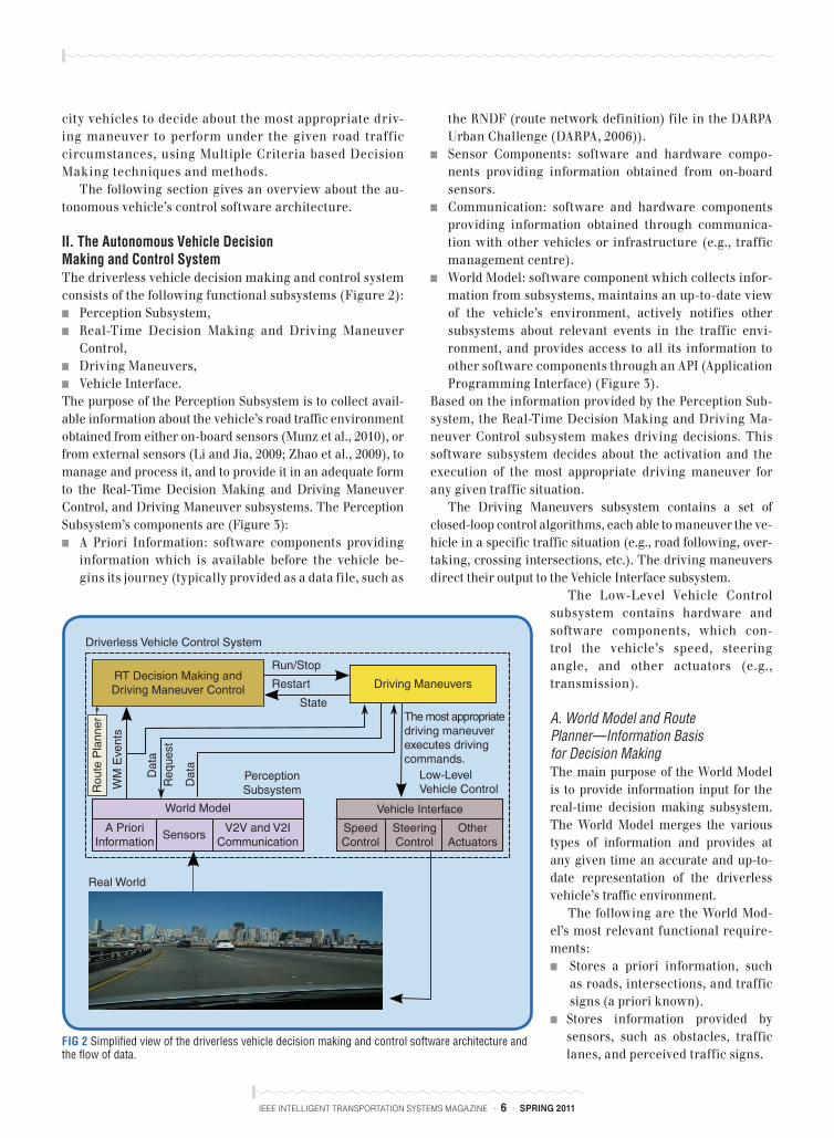
II. The Autonomous Vehicle Decision Making and Control SystemThe driverless vehicle decision making and control system consists of the following functional subsystems (Figure 2):

■ Perception Subsystem, ■ Real-Time Decision Making and Driving Maneuver

Control, ■ Driving Maneuvers, ■ Vehicle Interface.

The purpose of the Perception Subsystem is to collect avail-able information about the vehicle’s road traffic environment obtained from either on-board sensors (Munz et al., 2010), or from external sensors (Li and Jia, 2009; Zhao et al., 2009), to manage and process it, and to provide it in an adequate form to the Real-Time Decision Making and Driving Maneuver Control, and Driving Maneuver subsystems. The Perception Subsystem’s components are (Figure 3):

■ A Priori Information: software components providing information which is available before the vehicle be-gins its journey (typically provided as a data file, such as

the RNDF (route network definition) file in the DARPA Urban Challenge (DARPA, 2006)).

■ Sensor Components: software and hardware compo-nents providing information obtained from on-board sensors.

■ Communication: software and hardware components providing information obtained through communica-tion with other vehicles or infrastructure (e.g., traffic management centre).

■ World Model: software component which collects infor-mation from subsystems, maintains an up-to-date view of the vehicle’s environment, actively notifies other subsystems about relevant events in the traffic envi-ronment, and provides access to all its information to other software components through an API (Application Programming Interface) (Figure 3).

Based on the information provided by the Perception Sub-system, the Real-Time Decision Making and Driving Ma-neuver Control subsystem makes driving decisions. This software subsystem decides about the activation and the execution of the most appropriate driving maneuver for any given traffic situation.

The Driving Maneuvers subsystem contains a set of closed-loop control algorithms, each able to maneuver the ve-hicle in a specific traffic situation (e.g., road following, over-taking, crossing intersections, etc.). The driving maneuvers direct their output to the Vehicle Interface subsystem.

The Low-Level Vehicle Control subsystem contains hardware and software components, which con-trol the vehicle’s speed, steering angle, and other actuators (e.g., transmission).

A. World Model and Route Planner—Information Basis for Decision Making The main purpose of the World Model is to provide information input for the real-time decision making subsystem. The World Model merges the various types of information and provides at any given time an accurate and up-to-date representation of the driverless vehicle’s traffic environment.

The following are the World Mod-el’s most relevant functional require-ments: ■ Stores a priori information, such

as roads, intersections, and traffic signs (a priori known).

■ Stores information provided by sensors, such as obstacles, traffic lanes, and perceived traffic signs.

FIG 2 Simplified view of the driverless vehicle decision making and control software architecture and the flow of data.

Driverless Vehicle Control System

RT Decision Making andDriving Maneuver Control

Run/Stop

Restart

State

Driving Maneuvers

The most appropriatedriving maneuverexecutes drivingcommands.

Low-LevelVehicle Control

Vehicle Interface

SpeedControl

SteeringControl

OtherActuators

V2V and V2ICommunication

PerceptionSubsystemW

M E

vent

s

Dat

aR

eque

st

Dat

a

Rou

te P

lann

er

World Model

SensorsA Priori

Information

Real World


■ Stores information obtained through communication with other vehicles or a traffic management center.

■ Cyclicly merges and updates the a priori information with the information obtained continuously from sen-sor and communication components.

■ Calculates cyclicly the relationships between the stored entities. For example, if sufficient data is available, the World Model determines the positions of the current road, the current traffic lane, obstacles on the current road, the type of obstacles on the current lane/road, and distances to obstacles.

■ Notifies other subsystems of relevant events in the traffic environment through an asynchronous mechanism.

■ Provides other subsystems complete access to all stored information by replying to synchronous data requests (Figure 3).

The World Model API consists of two entities, each imple-menting a different concept:

■ World Model Events, ■ Object-oriented data structure.

A World Model Event represents a discrete event which signals the availability of certain information, that certain conditions are suddenly met, or the occurrence of a certain event happening in the real world. The principle is along the line of Discrete Event Systems (Cassandras and Lafor-tune, 2008). The state of a World Model Event is modeled as a boolean variable.

World Model Events are used to notify other software components about the state of certain predefined con-ditions, which are relevant for the execution of driving maneuvers. The specification of each driving maneuver requires that, in order to be safely performed, certain con-ditions have to be met, or certain information has to be available. Such conditions can be, for instance, related to traffic situations (e.g., “pedestrian n meters in front of the vehicle”), but might as well be related to the availability of sensor information (e.g., “GPS localization available”).

The World Model Events enable a flexible way to define what information is relevant for decision making, and pro-vide an easy mechanism for quick information exchange between the World Model and the Real-Time Decision Making subsystem.

The state of all defined World Model Events is provided as a k-tuple:

WMevents 5 1w1, w2, c, wk 2 : wl [ 5true, false6, (1)

where each element wl 1 l 5 1, 2, c, k 2 represents an event. The k-tuple WMevents is updated cyclicly, and other (as

observer registered) software components are actively no-tified about the occurrence of certain conditions as defined for each event. A timestamp assigned to the event tuple may be used to ensure that the update operation is performed within the required time intervals.

Besides World Model Events, the World Model pro-vides other software components full access to all its data through an object-oriented data structure. Further details about the developed World Model have been published in (Furda and Vlacic, 2010).

The Route Planner: In many situations, the planned route has a significant impact on decision making. For in-stance overtaking a slower vehicle just before a planned turn may not be adequate. Therefore, a route planner pro-vides the decision making module with information about the prospective planned route, well in advance (e.g., 50–150 m) before required turns and changes of direction.

Without the loss of generality, we require that the pro-vided route planner information is specified as an element of the set

Droute 5 5 forward_straight, forward_right, forward_left, turn_around6, (2)

where each element indicates the future travel direc-tion. The direction forward_straight indicates that the planned route is to follow the current road, forward_right and forward_left indicate a turn in the near future, while turn_around indicates that the next destination lies behind and a U-turn is necessary.

FIG 3 World Model Input and Output.

AsynchronousNotificationWM Events

SynchronousData Exchange

Roa

ds, I

nter

sect

ions

Sensor DataFusion

Data Processing,Perception,

Classification

Vehicles,Pedestrians,Traffic Lanes,Traffic Signs

V2I

Com

mun

icat

ion

V2V

Com

mun

icat

ion

Sen

sor

n

Sen

sor

2

Sen

sor

1

A P

riori

Info

rmat

ion

World Model

. . .


B. Driving Maneuvers—The Decision AlternativesDriving maneuvers are closed-loop control algorithms, each capable of maneuvering the driverless vehicle over a time period or distance. All driving maneuvers are struc-tured in a common way. Their operational behaviors are modeled as deterministic finite automata (Hopcroft et al., 2007; Cassandras and Lafortune, 2008) (Figure 4):

■ a start state q0 is the waiting or idle state, in which the automaton is waiting for the Run signal.

■ a set of Run states Qrun 5 5q1r, q2

r, c, qnr6 ( Q, each repre-

senting a phase of a driving maneuver, perform the ma-neuvering of the vehicle. Each of them includes checking of necessary preconditions, such as the availability of re-quired information and safety conditions. As long as the defined preconditions are met, the Run states execute closed-loop control algorithms. Otherwise, if certain preconditions are not met, the Error symbol is generated, and the automaton changes into the error state qE.

■ two final states 5qF, qE6 5 F. The final state qF (finished) represents a successful completion of the driving ma-neuver, while the error state qE (error) signals that the driving maneuver has been aborted due to an error or some other reason.

■ a set of input symbols S, which consists of at least the symbols: Run, Stop, Restart, Error, and the state transi-tion function d : Q 3 S S Q.

Furthermore, each driving maneuver offers a set of execu-tion alternatives, which are specified by discrete param-eters. Parameters are reference values (set points) for the closed-loop control algorithms implemented in the Run states Qrun. For instance, an overtaking maneuver requires the specification of parameters which define how close and

how fast the driverless vehicle should approach the front vehicle before changing lanes.

III. Real-Time Decision MakingBased on the elaborated prerequisites, the decision making task can be specified as follows:

■ a set Mall 5 5m1, m2, cmn6, n [ N1, of all available driv-ing maneuvers which can be performed by the driverless vehicle,

■ a k-tuple 1w1, w2, c, wk 2 [ Wevents of World Model Events, wl [ 50, 16, l 5 1, 2, c, k

■ a route planner direction indication di [ Droute.The general task of decision making in this context is to iden-tify the most appropriate driving maneuver mmost_appr. [ Mall, which leads to a driverless vehicle driving behavior con-forming to the specification.

A. Decomposition into SubtasksThe general decision making task is decomposed into the following two consecutive stages: 1) Decision regarding feasible, safety-critical driving ma-

neuvers subject to World Model Events and route planner indication. A driving maneuver is defined as feasible if it can be safely performed in a specific traffic situation, and is conforming to the road traffic rules. In order to ensure safety, it is assumed that the autonomous vehicle will always obey the traffic rules, which however might need to be adapted for such vehicles in the future. In any traffic situation, there can be multiple feasible driving maneuvers (e.g., overtaking a stopped vehicle or wait-ing for it to continue driving).

2) Decision regarding the most appropriate driving ma-neuver. This stage selects and starts the execution of one single driving maneuver, which is selected as the most appropriate for the specific traffic situation. Since only those driving maneuvers are considered in this stage which have been selected as feasible (and there-fore safe), this stage is not safety-critical because it does not include any decision making attributes which affect safety.

The decomposition into two stages with different objectives leads to subtasks with manageable complexity, enabling the verification and testing of each stage in particular. While the main focus of the first stage is to determine which driving maneuvers are safe and conform to traffic rules, the second, non safety critical decision stage focuses on improving comfort and efficiency.

The entire decision making process (i.e., the two stag-es) is executed cyclicly. Once a driving maneuver has been activated, it remains active within the given cycle, and it will be executed as long as its execution is feasible, until it finishes in one of its two final states qF or qE. If a driving

1N 5 set of natural numbers.

Run

Run

Restart

Restart

Stop

Error

Error

Error

Stop

Stop

Run

Run

Next_Phase

Next_Phase

Next_Phase

q0

qF

qE

q1r

qNr

q2r

FIG 4 A driving maneuver finite automaton with multiple Run states. The number of Run states qi

r, i 5 1, 2, cN equals the number of driving maneuver phases.


maneuver becomes infeasible during its execution, the decision making subsystem is able to abort its execu-tion, and activate another driving ma-neuver instead.

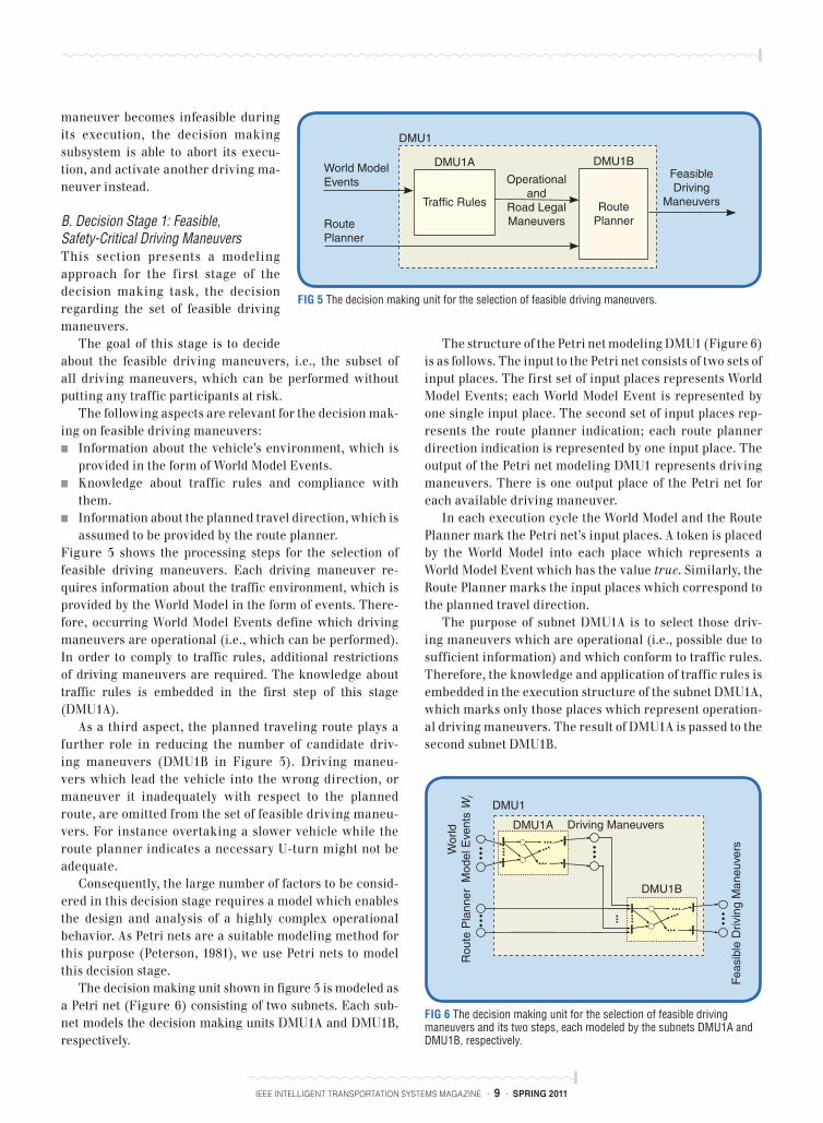
B. Decision Stage 1: Feasible, Safety-Critical Driving ManeuversThis section presents a modeling approach for the first stage of the decision making task, the decision regarding the set of feasible driving maneuvers.

The goal of this stage is to decide about the feasible driving maneuvers, i.e., the subset of all driving maneuvers, which can be performed without putting any traffic participants at risk.

The following aspects are relevant for the decision mak-ing on feasible driving maneuvers:

■ Information about the vehicle’s environment, which is provided in the form of World Model Events.

■ Knowledge about traffic rules and compliance with them.

■ Information about the planned travel direction, which is assumed to be provided by the route planner.

Figure 5 shows the processing steps for the selection of feasible driving maneuvers. Each driving maneuver re-quires information about the traffic environment, which is provided by the World Model in the form of events. There-fore, occurring World Model Events define which driving maneuvers are operational (i.e., which can be performed). In order to comply to traffic rules, additional restrictions of driving maneuvers are required. The knowledge about traffic rules is embedded in the first step of this stage (DMU1A).

As a third aspect, the planned traveling route plays a further role in reducing the number of candidate driv-ing maneuvers (DMU1B in Figure 5). Driving maneu-vers which lead the vehicle into the wrong direction, or maneuver it inadequately with respect to the planned route, are omitted from the set of feasible driving maneu-vers. For instance overtaking a slower vehicle while the route planner indicates a necessary U-turn might not be adequate.

Consequently, the large number of factors to be consid-ered in this decision stage requires a model which enables the design and analysis of a highly complex operational behavior. As Petri nets are a suitable modeling method for this purpose (Peterson, 1981), we use Petri nets to model this decision stage.

The decision making unit shown in figure 5 is modeled as a Petri net (Figure 6) consisting of two subnets. Each sub-net models the decision making units DMU1A and DMU1B, respectively.

The structure of the Petri net modeling DMU1 ( Figure 6) is as follows. The input to the Petri net consists of two sets of input places. The first set of input places represents World Model Events; each World Model Event is represented by one single input place. The second set of input places rep-resents the route planner indication; each route planner direction indication is represented by one input place. The output of the Petri net modeling DMU1 represents driving maneuvers. There is one output place of the Petri net for each available driving maneuver.

In each execution cycle the World Model and the Route Planner mark the Petri net’s input places. A token is placed by the World Model into each place which represents a World Model Event which has the value true. Similarly, the Route Planner marks the input places which correspond to the planned travel direction.

The purpose of subnet DMU1A is to select those driv-ing maneuvers which are operational (i.e., possible due to sufficient information) and which conform to traffic rules. Therefore, the knowledge and application of traffic rules is embedded in the execution structure of the subnet DMU1A, which marks only those places which represent operation-al driving maneuvers. The result of DMU1A is passed to the second subnet DMU1B.

DMU1

DMU1A Driving Maneuvers

DMU1B

Fea

sibl

e D

rivin

g M

aneu

vers

Rou

te P

lann

erW

orld

Mod

el E

vent

s W

i

FIG 6 The decision making unit for the selection of feasible driving maneuvers and its two steps, each modeled by the subnets DMU1A and DMU1B, respectively.

DMU1

DMU1A DMU1BWorld ModelEvents

RoutePlanner

Traffic Rules RoutePlanner

FeasibleDriving

Maneuvers

Operationaland

Road LegalManeuvers

FIG 5 The decision making unit for the selection of feasible driving maneuvers.


The purpose of the subnet DMU1B is to filter out those driving maneuvers which were determined as operational by DMU1A, however which do not lead the vehicle into the direction indicated by the route planner. Therefore, the sub-net DMU1B receives both inputs from the route planner and inputs from the subnet DMU1A. After its execution, DMU1B places a token into each Petri net output place which rep-resents a driving maneuver which is both operational and according to the route planner indication.

After the execution of the complete Petri net DMU1, only those Petri net output places are marked, which represent feasible driving maneuvers (i.e., operational and according to the route planner). After each decision making cycle, all marked places of the Petri net are cleared, and a new deci-sion making cycle begins.

In the current prototype implementation, since this is the safest option, in the unlikely event that there is no fea-sible driving maneuver, the vehicle stops, and waits for a maneuver to become feasible. However, with a complete system specification, which defines how the vehicle should respond to any traffic situation, and a complete list of re-quired driving maneuvers, this will be avoided.

Besides its scalability, the main benefit of the Petri net model is that it allows to model, analyze, and verify the correctness of a very complex operational behavior of the first, safety-critical decision making stage, including a large number of World Model events (Petri net input places), which represent real-world events in the vehicle’s traffic environment. This allows the decision making subsystem to deal with very complex real-world traffic situations. Fur-thermore, since the Petri net structure is decoupled from the control software implementation, and loaded from an external XML file, only its execution is implemented in the vehicle control software source code. Consequently, chang-es of the decision making operational behavior (in the Petri net XML file) do not require changes of the source code, and this in turn minimizes the possibility to introduce new software errors.

C. Decision Stage 2: Selecting the Most Appropriate Driving Maneuver Using MCDMThe goal of the second decision making stage is to select and execute the most appropriate alternative from those driving maneuvers which have been determined to be fea-sible in the current traffic situation.

Each of the feasible driving maneuvers offers multiple execution alternatives, which can be selected through discrete driving maneuver parameters. For instance, the overtaking maneuver could be performed at low or high speed, in distant or close proximity to the front vehicle, and on the right or left hand side. In order to select the most ap-propriate driving maneuver, and for it the most appropriate execution alternative, we apply Multiple Criteria Decision Making (MCDM) as follows.

Objectives: we define a hierarchy of objectives start-ing from a main, most general driving objective, which is then further successively broken down into more spe-cific and therefore more operational objectives on lower hierarchy levels. Eventually, the bottom level of the ob-jective hierarchy contains only objectives objj which are fully operational and which are measurable through their attributes.

The most general objective for autonomous driving is to safely reach the specified destination. More precisely, this objective is broken down into a lower hierarchy level containing more specific objectives, which specify how to achieve the objective of the higher level.

Thus, we define the following example objective hierar-chy consisting of four (k 5 4) level 2 objectives:

■ Drive to destination safely 5: obj Level1 ■ Stay within road boundaries 5: obj1

Level2 keep distance to right boundary J attr1 keep distance to left boundary J attr2

■ Keep safety distances 5: obj2Level2

keep distance to front vehicle J attr3 keep distance to moving obstacles J attr4 keep distance to static obstacles J attr5

■ Do not collide 5: obj3Level2

keep minimum distance to obstacles J attr6 drive around obstacles J attr7 avoid sudden braking J attr8 avoid quick lane changes J attr9

■ Minimize waiting time 5: obj4Level2

maintain minimum speed J attr10 avoid stops J attr11

Attributes: a set of measurable attributes

5attr1, attr2, c, attrp6, p [ N (3)

is assigned to each objective on the lowest hierarchy level (in our example p 5 11). An attribute is a prop-erty of a specific objective. In order to define various levels of importance, weights may be assigned to each attribute.

Alternatives: in the context of our application, decision al-ternatives correspond to the execution of driving maneuvers. Therefore, in a first step, we regard each element of the set of driving maneuvers 5M1, M2, c, Mn6 1n [ N 2 to be an ele-ment of the set of alternatives A:

A 5 5M1, M2, c, Mn6 (4)

However, each driving maneuver Mm 11 # m # n 2 offers one

or multiple execution alternatives by specifying discrete parameter values (e.g., fast/slow, close/far, etc.). The driv-ing maneuver parameters correspond in MCDM terms to decision variables, where each alternative is represented by a decision variable vector.


We obtain:

M1 5 5M11, M2

1, c, Mj16

M2 5 5M12, M2

2, c, Mk26

(Mn 5 5M1

n, M2n, c, Ml

n6

(5)

where n denotes the number of driving maneuvers, and j, k, l the number of execution alternatives for the maneuvers M1, M2, and Mn respectively.

Therefore, the set of alternatives A contains all execu-tion alternatives of all n driving maneuvers:

A 5 dn

m51 M m

5 5M11, M2

1, c, Mj1, M1

2, c, Mk2,c, M1

n,c Mln6 (6)

For the sake of readability, we denote all alternatives as:

A 5 5a1, a2, c, aq6, 1q 5 j 1 k 1c1 l 2 (7)

Utility Functions: utility functions f1 1ar 2 , c, fp 1ar 2 spec-ify the level of achievement of an objective by an al-ternative ar [ A 1r [ 31, q 4 2 with respect to each of the p attributes.

For each attribute attri 1 i [ 31, p 4 2 , we define a utility function fattri

5 fi:

fi : A S 30, 1 4 (8)

Consequently, defining utility functions fi for all alterna-tives a1, a2, c, aq and all attributes attri 1 i [ 31, p 4 2 results in the following decision matrix:

ar attr1 attr2c attrp

a1 f1 1a1 2 f2 1a1 2 c fp 1a1 2

a2 f1 1a2 2 f2 1a2 2 c fp 1a2 2

( ( ( ( (aq f1 1aq 2 f2 1aq 2 c fp 1aq 2

The remaining task is to calculate a best solution among the feasible alternatives. A variety of MCDM methods can be applied in order to solve this problem, such as dominance methods, satisficing methods, sequential elimination meth-ods, or scoring methods (Yoon and Hwang, 1995).

In the following example we choose a widely used scoring method, the Simple Additive Weighting Method, in which the value V 1ar 2 of an alternative ar is calculated by multiplying the utility function values with the attribute weights and then totaling the products over all attributes (see equation 11) (Yoon and Hwang, 1995). The alterna-tive with the highest value is then chosen. Besides being easy to calculate, the Simple Additive Weighting Method allows to indicate the level of importance of certain attri-butes using weights.

Instead of using the Simple Additive Weighting Meth-od, other methods can also be applied, in order to seek a Pareto optimal (noninferior) solution, i.e., a solution where no other alternative will improve one attribute without degrading at least another attribute (Chankong and Haimes, 1983). This comparison has to therefore be performed in the context of finding safety-critical solu-tions. Also, having in mind the decision making algo-rithm’s hard real-time requirements which in turn are safety-crucial, the benefits of finding a Pareto optimal solution will be achieved if and only if the necessary com-puting power is available.

D. Example for Decision Stage 2In this example we assume the traffic situation where a driverless vehicle decides about passing a stopped vehicle. Without oncoming traffic, the first decision making stage determined the following two driving maneuvers as fea-sible: Passing the stopped vehicle, or Stop&Go (i.e., waiting behind the temporarily stopped vehicle).

For the sake of simplicity, we assume that only the following few execution alternatives for the two driving maneuvers are possible:

■ Passing maneuver M1: ■ a1 J speed 5 slow, lateral distance 5 small ■ a2 J speed 5 slow, lateral distance 5 large ■ a3 J speed 5 fast, lateral distance 5 small ■ a4 J speed 5 fast, lateral distance 5 large

■ Stop and Go maneuver M2: ■ a5 J distance to front vehicle 5 small ■ a6 J distance to front vehicle 5 largeConsequently, the set of feasible alternatives is:

A 5 5a1, a2, c, a66 (9)

The utility functions fi 1A 2 evaluate the achievement level of each attribute i for each of the 6 alternatives. In order to allow comparisons between the levels of achievement of different objectives, the values of the utility functions fi are scaled to a common measurement scale, the interval of real numbers between 0 and 1. We define:

fi [ 30, 1 4 ( R, (10)

where the value 1 denotes the optimal achievement of an objective, while 0 denotes that the objective is not achieved at all.

We define the utility functions as follows. Each of the 6 alternatives are rated regarding on how well they fulfill the driving objectives on the lowest hierarchy level. We rate the alternatives on a scale from 0 to 1, where:

■ 1 denotes optimal fulfillment of the objective, ■ 0.75 denotes good fulfillment, ■ 0.5 denotes indifference,


■ 0.25 denotes bad fulfillment, ■ 0 denotes unsatisfactory fulfillment.

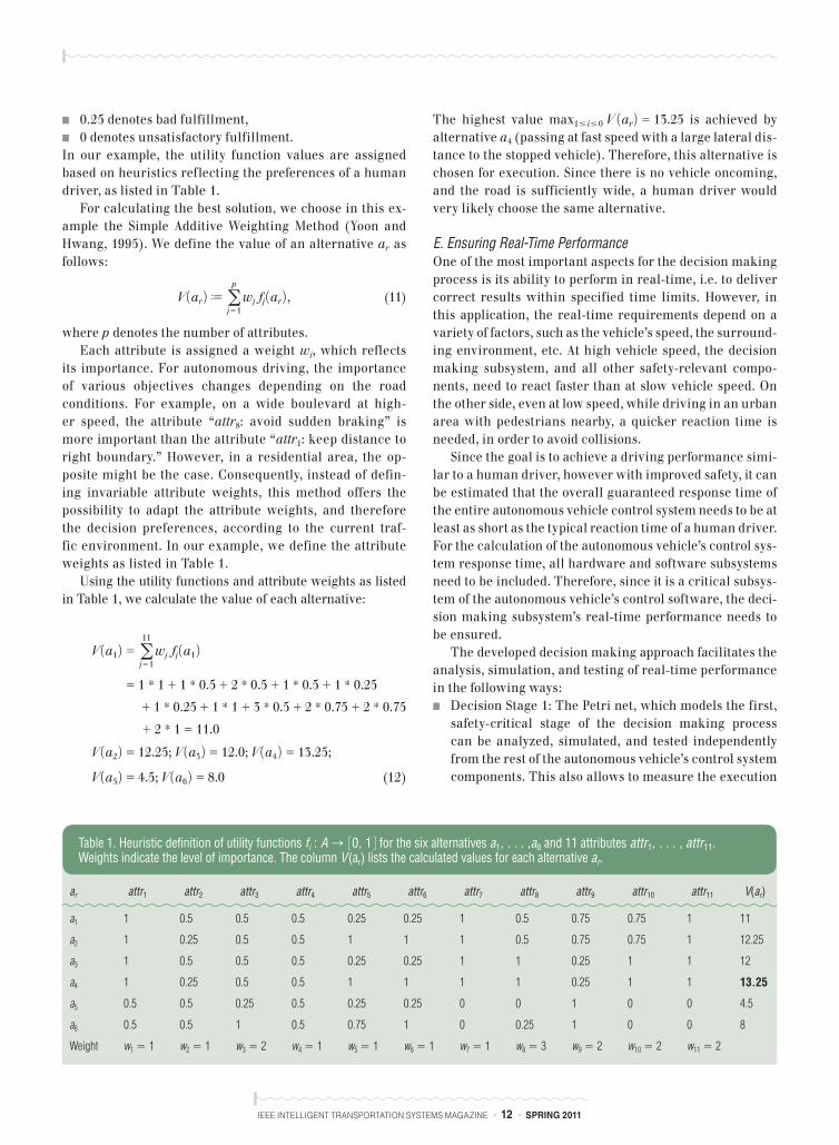
In our example, the utility function values are assigned based on heuristics reflecting the preferences of a human driver, as listed in Table 1.

For calculating the best solution, we choose in this ex-ample the Simple Additive Weighting Method (Yoon and Hwang, 1995). We define the value of an alternative ar as follows:

V 1ar 2 J ap

j51wj fj 1ar 2 , (11)

where p denotes the number of attributes. Each attribute is assigned a weight wj, which reflects

its importance. For autonomous driving, the importance of various objectives changes depending on the road conditions. For example, on a wide boulevard at high-er speed, the attribute “attr8: avoid sudden braking” is more important than the attribute “attr1: keep distance to right boundary.” However, in a residential area, the op-posite might be the case. Consequently, instead of defin-ing invariable attribute weights, this method offers the possibility to adapt the attribute weights, and therefore the decision preferences, according to the current traf-fic environment. In our example, we define the attribute weights as listed in Table 1.

Using the utility functions and attribute weights as listed in Table 1, we calculate the value of each alternative:

V 1a1 2 5 a11

j51wj fj 1a1 2

5 1 * 1 1 1 * 0.5 1 2 * 0.5 1 1 * 0.5 1 1 * 0.25

1 1 * 0.25 1 1 * 1 1 3 * 0.5 1 2 * 0.75 1 2 * 0.75

1 2 * 1 5 11.0

V 1a2 2 5 12.25; V 1a3 2 5 12.0; V 1a4 2 5 13.25;

V 1a5 2 5 4.5; V 1a6 2 5 8.0 (12)

The highest value max1# i#0 V 1ar 2 5 13.25 is achieved by alternative a4 (passing at fast speed with a large lateral dis-tance to the stopped vehicle). Therefore, this alternative is chosen for execution. Since there is no vehicle oncoming, and the road is sufficiently wide, a human driver would very likely choose the same alternative.

E. Ensuring Real-Time PerformanceOne of the most important aspects for the decision making process is its ability to perform in real-time, i.e. to deliver correct results within specified time limits. However, in this application, the real-time requirements depend on a variety of factors, such as the vehicle’s speed, the surround-ing environment, etc. At high vehicle speed, the decision making subsystem, and all other safety-relevant compo-nents, need to react faster than at slow vehicle speed. On the other side, even at low speed, while driving in an urban area with pedestrians nearby, a quicker reaction time is needed, in order to avoid collisions.

Since the goal is to achieve a driving performance simi-lar to a human driver, however with improved safety, it can be estimated that the overall guaranteed response time of the entire autonomous vehicle control system needs to be at least as short as the typical reaction time of a human driver. For the calculation of the autonomous vehicle’s control sys-tem response time, all hardware and software subsystems need to be included. Therefore, since it is a critical subsys-tem of the autonomous vehicle’s control software, the deci-sion making subsystem’s real-time performance needs to be ensured.

The developed decision making approach facilitates the analysis, simulation, and testing of real-time performance in the following ways:

■ Decision Stage 1: The Petri net, which models the first, safety-critical stage of the decision making process can be analyzed, simulated, and tested independently from the rest of the autonomous vehicle’s control system components. This also allows to measure the execution

ar attr1 attr2 attr3 attr4 attr5 attr6 attr7 attr8 attr9 attr10 attr11 V(ar)

a1 1 0.5 0.5 0.5 0.25 0.25 1 0.5 0.75 0.75 1 11

a2 1 0.25 0.5 0.5 1 1 1 0.5 0.75 0.75 1 12.25

a3 1 0.5 0.5 0.5 0.25 0.25 1 1 0.25 1 1 12

a4 1 0.25 0.5 0.5 1 1 1 1 0.25 1 1 13.25

a5 0.5 0.5 0.25 0.5 0.25 0.25 0 0 1 0 0 4.5

a6 0.5 0.5 1 0.5 0.75 1 0 0.25 1 0 0 8

Weight w1 5 1 w2 5 1 w3 5 2 w4 5 1 w5 5 1 w6 5 1 w7 5 1 w8 5 3 w9 5 2 w10 5 2 w11 5 2

Table 1. Heuristic definition of utility functions fi : A S 30, 1 4 for the six alternatives a1, c,a6 and 11 attributes attr1, c, attr11. Weights indicate the level of importance. The column V(ar) lists the calculated values for each alternative ar.


times for the Petri net execution on the actual comput-ing system, including the worst-case scenarios.

■ Decision Stage 2: Although the second decision mak-ing stage does not include safety-critical attributes, its real-time performance ability does have an effect on the entire decision making process. Therefore, the number of MCDM objectives, the choice of the MCDM method, and for instance the calculation cost for seeking Pare-to optimal solutions, need to be in line with real-time requirements. For this reason, the Simple Additive Weighting Method has been chosen in the implementa-tion, due to its low calculation costs.

F. Real-Time Performance MeasurementsIn order to assess the real-time performance of the first, Petri Net based decision making stage, the Petri net imple-mentation has been tested and its execution performance has been measured independently from the vehicle control software. For this purpose, two different Petri Net struc-tures have been created, which reflect the building blocks of a complex decision making net:

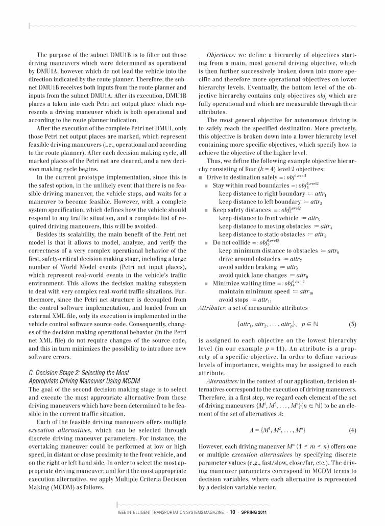
■ A Petri Net with a single transition with multiple inputs and multiple outputs (Figure 7), and;

■ A Petri net with multiple transitions with single inputs and single outputs (Figure 8).

Single Transition with Multiple Inputs/Multiple Outputs. The first measured Petri Net structure consists of a single tran-sition with a multiple inputs and multiple outputs (Figure 7). In order to assess the execution time of this structure, a large number of input places and output places has been cre-ated, the input places have been marked, and the execution time for the execution of the Petri Net (i.e., the firing of the single transition) has been measured.

Table 2 shows the average execution times with respect to the number of input and output places, as well as the time required to remove all Petri Net markings after the execution of the entire Petri Net (Reset). The removal of re-maining markings after each execution cycle is required, in order to reset the Petri Net to its original state before the execution of a new decision making cycle.

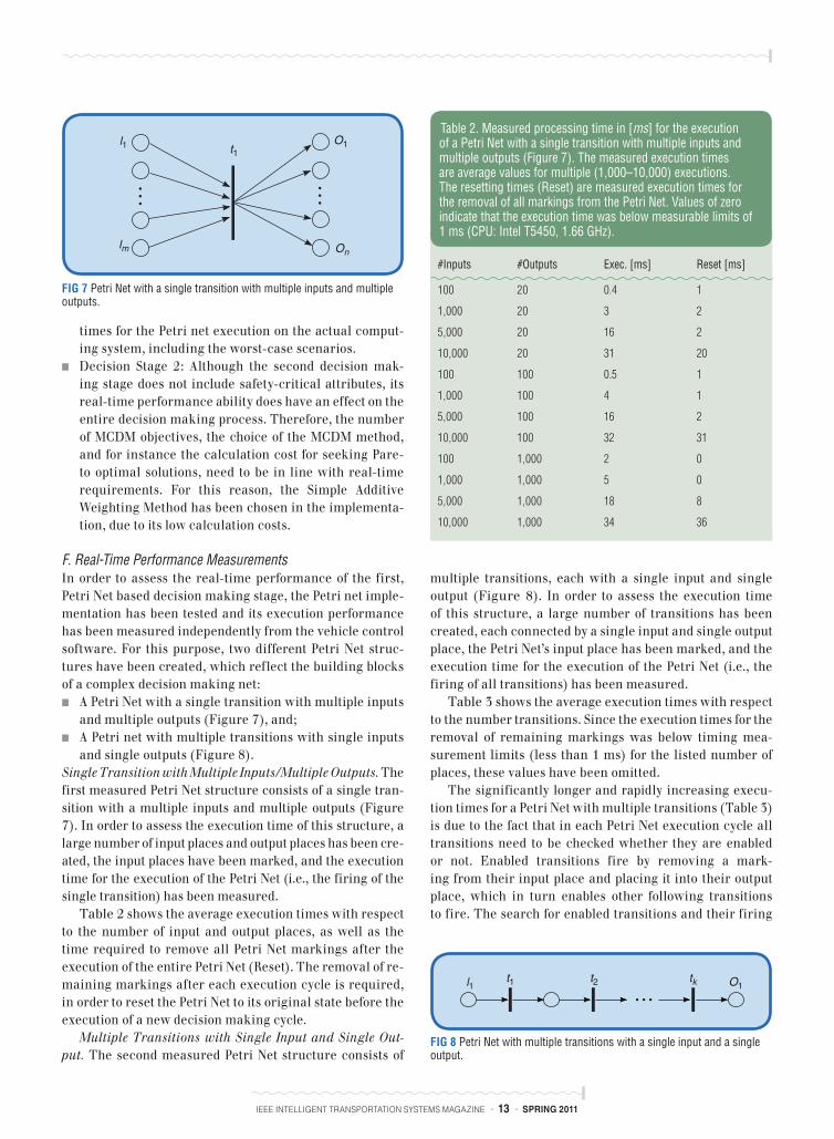
Multiple Transitions with Single Input and Single Out-put. The second measured Petri Net structure consists of

multiple transitions, each with a single input and single output (Figure 8). In order to assess the execution time of this structure, a large number of transitions has been created, each connected by a single input and single output place, the Petri Net’s input place has been marked, and the execution time for the execution of the Petri Net (i.e., the firing of all transitions) has been measured.

Table 3 shows the average execution times with respect to the number transitions. Since the execution times for the removal of remaining markings was below timing mea-surement limits (less than 1 ms) for the listed number of places, these values have been omitted.

The significantly longer and rapidly increasing execu-tion times for a Petri Net with multiple transitions (Table 3) is due to the fact that in each Petri Net execution cycle all transitions need to be checked whether they are enabled or not. Enabled transitions fire by removing a mark-ing from their input place and placing it into their output place, which in turn enables other following transitions to fire. The search for enabled transitions and their firing

FIG 7 Petri Net with a single transition with multiple inputs and multiple outputs.

l1

lm On

O1t1

l1t1 O1

t2 tk

FIG 8 Petri Net with multiple transitions with a single input and a single output.

#Inputs #Outputs Exec. [ms] Reset [ms]

100 20 0.4 1

1,000 20 3 2

5,000 20 16 2

10,000 20 31 20

100 100 0.5 1

1,000 100 4 1

5,000 100 16 2

10,000 100 32 31

100 1,000 2 0

1,000 1,000 5 0

5,000 1,000 18 8

10,000 1,000 34 36

Table 2. Measured processing time in [ms] for the execution of a Petri Net with a single transition with multiple inputs and multiple outputs (Figure 7). The measured execution times are average values for multiple (1,000–10,000) executions. The resetting times (Reset) are measured execution times for the removal of all markings from the Petri Net. Values of zero indicate that the execution time was below measurable limits of 1 ms (CPU: Intel T5450, 1.66 GHz).


is executed until there are no more enabled transitions, which results in increased processing times.

The measured execution time values listed in tables 2 and 3 can be used to estimate the maximum required pro-cessing times for a decision making Petri Net in a worst case scenario.

For example, the execution for a Petri Net consisting of 200 transitions with each 1000 input and 100 output plac-es, will require on this specific hardware in a worst case ( Table 2): 200 * 4 ms 5 800 ms.

Additionally, the time required to reset the net (i.e., to clear all markings) is around 1 ms for each transition. Therefore, the execution time for the entire Petri Net on this specific CPU is: 800 ms 1 1 ms * 200 5 1000 ms

Although the implemented prototype system does not include all required aspects for an autonomous vehicle to be fully operational in real-world traffic, the conducted tests attest that the developed approach is suitable to ful-fill real-time requirements. So far, the developed software has been successfully tested on a Windows Vista notebook

PC with an Intel T5450 CPU at 1.66 GHz with satisfactory results for the low vehicle speed of around 1 m/s. On this low-end notebook CPU and general purpose (i.e., non- real time) operating system, the decision making process was executed at 1–2 Hz, concurrently to all other vehicle con-trol tasks on the same CPU. During these tests, the CPU load was relatively low (30–40%), which indicates that the decision making process, if executed on a dedicated CPU, under a real-time operating system, is able fulfill the real-time requirements for much higher vehicle speeds.

G. Error RecoveryDue to quickly and unexpectedly changing traffic condi-tions, in some situations, the decision making subsystem may need to abort the execution of certain driving maneu-vers (such as overtaking), and switch to the execution of driving maneuvers specifically developed for error recov-ery. However, since the structure of error recovery driving maneuvers is identical to normal driving maneuvers, the process of error recovery does not require any changes of the decision making approach.

One of the challenges for the near future, and a so far not addressed question, is the development of a complete and detailed system specification for autonomous driving in ur-ban traffic conditions, which foresees and includes how to deal with such unexpected traffic conditions.

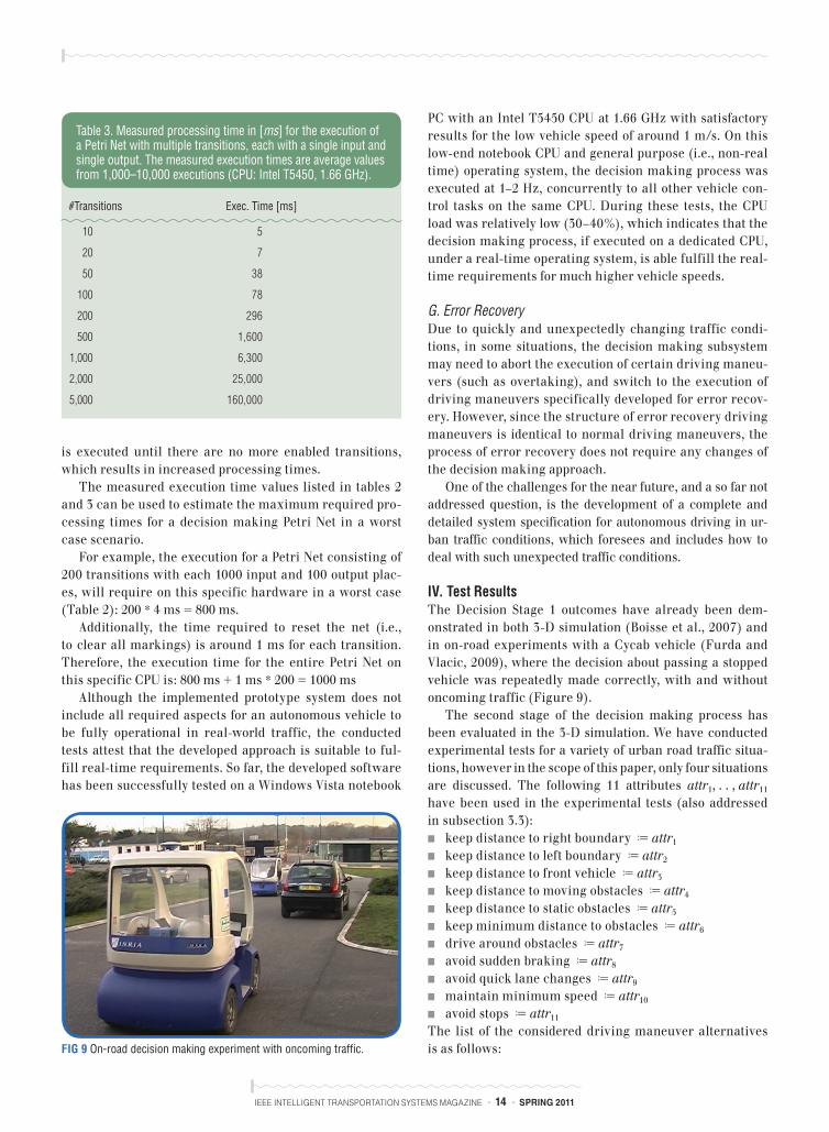
IV. Test ResultsThe Decision Stage 1 outcomes have already been dem-onstrated in both 3-D simulation (Boisse et al., 2007) and in on-road experiments with a Cycab vehicle (Furda and Vlacic, 2009), where the decision about passing a stopped vehicle was repeatedly made correctly, with and without oncoming traffic (Figure 9).

The second stage of the decision making process has been evaluated in the 3-D simulation. We have conducted experimental tests for a variety of urban road traffic situa-tions, however in the scope of this paper, only four situations are discussed. The following 11 attributes attr1, . . , attr11 have been used in the experimental tests (also addressed in subsection 3.3):

■ keep distance to right boundary J attr1 ■ keep distance to left boundary J attr2 ■ keep distance to front vehicle J attr3 ■ keep distance to moving obstacles J attr4 ■ keep distance to static obstacles J attr5 ■ keep minimum distance to obstacles J attr6 ■ drive around obstacles J attr7 ■ avoid sudden braking J attr8 ■ avoid quick lane changes J attr9 ■ maintain minimum speed J attr10 ■ avoid stops J attr11

The list of the considered driving maneuver alternatives is as follows: FIG 9 On-road decision making experiment with oncoming traffic.

#Transitions Exec. Time [ms]

10 5

20 7

50 38

100 78

200 296

500 1,600

1,000 6,300

2,000 25,000

5,000 160,000

Table 3. Measured processing time in [ms] for the execution of a Petri Net with multiple transitions, each with a single input and single output. The measured execution times are average values from 1,000–10,000 executions (CPU: Intel T5450, 1.66 GHz).


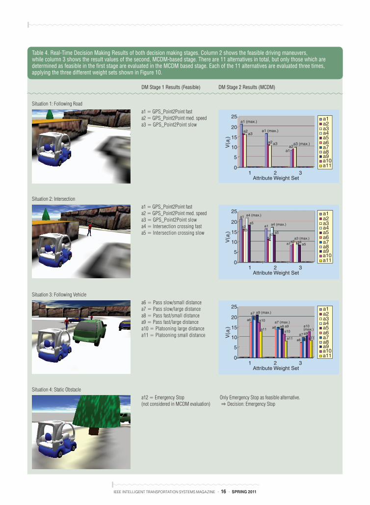
■ a1 5 GPS_Point2Point fast ■ a2 5 GPS_Point2Point medium speed ■ a3 5 GPS_Point2Point slow ■ a4 5 Intersection crossing fast ■ a5 5 Intersection crossing slow ■ a6 5 Pass slow/small distance ■ a7 5 Pass slow/large distance ■ a8 5 Pass fast/small distance ■ a9 5 Pass fast/large distance ■ a10 5 Platooning large distance ■ a11 5 Platooning small distance ■ a12 5 Emergency stop

In order to test the sensitivity of the developed Decision Stage 2 method, three different attribute weight distribution sets have been applied for each of these 11 attributes, as shown in Figure 10. The Weight Set 1 was chosen in such a way that the highest weight factors of 5 is assigned to both attributes 1 and 11, while the weight factor of 2.5 is assigned to attribute 6; the Weight Set 2 assigns increasing weight factors in steps of 0.5, while the Weight Set 3 assigns decreasing weight fac-tors in steps of 0.5.

The outcomes of the first decision making stage are pre-sented in Table 4, Column 2, as follows:

■ Situation 1: the autonomous vehicle is following a road, relatively far from the coming intersection. In this situa-tion, the first, Petri net based decision making stage has determined the driving maneuver for following a road us-ing GPS coordinates, and its three execution alternatives (i.e., fast, medium speed, slow), as feasible.

■ Situation 2: the autonomous vehicle is approaching an intersection, with a road crossing pedestrian. In addition to the road following maneuver, the first decision mak-ing determines the intersection crossing maneuver as feasible.

■ Situation 3: the autonomous vehicle is following another vehicle. The first decision making stage determines the driving maneuvers “Pass” and “Platooning” as feasible.

■ Situation 4: a static obstacle (a tree) is in front of the au-tonomous vehicle. The only feasible driving maneuver is the emergency stop.

The second, MCDM-based decision making stage calcu-lates the values V 1ai 2 for each of the feasible alternatives using Equation 11, which provided in this case the follow-ing results (Table 4, column 3):

■ Situation 1: the use of the Weight Set 1 and Weight Set 2 result in the alternative a1 to be most appropriate (i.e., maximum value), while the Weight Set 3 results in the alternative a3 to be the most appropriate.

■ Situation 2: the alternative a4 is the most appropriate for weight sets 1 and 2, while alternative a3 becomes the most appropriate if the Weight Set 3 is applied.

■ Situation 3: the use of the Weight Set 1 results in the decision to execute alternative a9, while alternatives a7 and a10 are chosen for weight sets 2 and 3 respectively.

■ Situation 4: the only feasible driving maneuver is the emergency stop. In our implementation the emergency stop is not evaluated by the MCDM based stage, but is in-stead immediately executed whenever it is determined to be the only feasible alternative.

As expected, whenever the World Model fails to provide accurate information, such as for instance information re-garding oncoming vehicles (e.g., Table 4, Situation 3), the first decision making stage may make the wrong decision about the feasible driving maneuvers. This error is then further passed on to the second stage, and may result in inappropriate or even unsafe driving decisions. Therefore, since it is mainly responsible for safety aspects, the first decision making stage has a crucial impact on the entire decision result.

On the other side, the MCDM results in Table 4 show that even when the attributes and utility functions of the second, MCDM based decision making stage have not been speci-fied appropriately, for instance by assigning weights too high to irrelevant attributes, the resulting driving decisions are still safe. For example, applying the first set of attribute weights in Situation 1 results in the decision to approach the intersection at fast speed (i.e., alternative 1), while applying the third attribute weight set results in the more appropri-ate decision to approach the intersection at a lower speed (i.e., alternative 3).

Consequently, the developed decision making approach delivers correct decision results under the following conditions:

■ accurate and sufficient information is provided by the World Model in real-time, especially regarding the MCDM attributes;

■ the Petri Net based logic of the first decision making stage is defined according to a complete specification (i.e., a specification which defines the decision logic for all urban traffic conditions);

■ the MCDM attributes and their weights are specified ac-cording to their importance as judged by the transport system experts.

FIG 10 MCDM attribute weight distributions applied to the 11 attributes.

54.5

43.5

32.5

21.5

10.5

01 2 3 4 5 6 7 8 9 10 11

Attribute Attri (i = 1...11)

Wei

ght F

acto

r

Weight Set 1Weight Set 2Weight Set 3


DM Stage 1 Results (Feasible) DM Stage 2 Results (MCDM)

Situation 1: Following Road a1 5 GPS_Point2Point fast a2 5 GPS_Point2Point med. speed a3 5 GPS_Point2Point slow

25

20

15

V(a

i)

10

5

01 2

Attribute Weight Set

a1 (max.)

a1 (max.)

a3 (max.)

a2

a2

a3

a3

a1

3

a1a2a3a4a5a6a7a8a9a10a11

a2

Situation 2: Intersection a1 5 GPS_Point2Point fast a2 5 GPS_Point2Point med. speed a3 5 GPS_Point2Point slow a4 5 Intersection crossing fast a5 5 Intersection crossing slow

25

20

15V

(ai)

10

5

01 2


a1

a1

a4 (max.)

a4 (max.)

a3 (max.)

a2

a2a2

a3

a5

a5a3

a1 a4a5

3


Situation 3: Following Vehiclea6 5 Pass slow/small distance a7 5 Pass slow/large distance a8 5 Pass fast/small distance a9 5 Pass fast/large distance a10 5 Platooning large distance a11 5 Platooning small distance

25

20

15

V(a

i)

10

5

01 2


a9 (max.)

a9

a7 (max.)a6

a6

a6

a7

a7a8

a8

a10

a10a11

a11 a11

3


a10(max.)

a9a8

Situation 4: Static Obstacle a12 5 Emergency Stop (not considered in MCDM evaluation)

Only Emergency Stop as feasible alternative.1 Decision: Emergency Stop

Table 4. Real-Time Decision Making Results of both decision making stages. Column 2 shows the feasible driving maneuvers, while column 3 shows the result values of the second, MCDM-based stage. There are 11 alternatives in total, but only those which are determined as feasible in the first stage are evaluated in the MCDM based stage. Each of the 11 alternatives are evaluated three times, applying the three different weight sets shown in Figure 10.


A. Future WorkWhile the prototype implementation and the presented eval-uation results demonstrate that the developed decision mak-ing approach is applicable and suitable, additional work is necessary in order to advance its development towards com-mercial real-world applications.

In order to obtain unconditional reliable decision mak-ing results, the following aspects need to be addressed by transportation system experts:

■ The minimal set of traffic environment information provided by the World Model needs to be refined in the context of making safe driving decisions.

■ The currently developed set of driving objectives needs to be expanded to unquestionably reflect the system specification.

■ Additional research is required for the development of a complete set of driving maneuvers for urban traffic, in order to enable real-time decision making and autono-mous driving in any situation.

V. ConclusionThis paper has addressed and presented a solution for the task of Real-Time Decision Making for autonomous city ve-hicles using Petri nets and MCDM. The decision making task has been divided into two consecutive stages. While the first decision making stage is safety-critical and focuses on se-lecting the feasible and safe driving maneuvers, the second decision making stage focuses on non safety-critical driving objectives, such as improving comfort and efficiency. We have demonstrated a solution for the first decision making stage based on Petri nets, and we have designed and devel-oped the MCDM model, which is applied in the second deci-sion making stage.

The application of MCDM methods for the second de-cision making stage enables the consideration of a large number of driving objectives, including possible conflicting ones, and leads to a powerful and flexible solution for non-simplified urban traffic conditions. Furthermore, compared to so far existing solutions, which were however intended only for simplified traffic conditions, the application of MCDM in this new research area offers a variety of benefits with respect to the problem specification, decision flexibil-ity, and scalability.

AcknowledgmentsWe would like to thank INRIA’s team IMARA for the financial support provided towards conducting the experimental work at their test track in Rocquencourt, France. We are particu-larly grateful to Dr. Michel Parent, Laurent Bouraoui, and Francois Charlot for their effort and assistance in performing the experiments.

About the AuthorsAndrei Furda received his Dipl.-In-form. degree in computer science from the University of Karlsruhe (TH), Ger-many, in 2004. Since 2006, he has been working towards his Ph.D. degree at the Intelligent Control Systems Laboratory (ICSL), Griffith University, Australia, un-der the supervision of Prof. Ljubo Vlacic.

Ljubo Vlacic is Professor and Director, Intelligent Control Systems Laboratory, Griffith University, Brisbane. In recogni-tion of his contributions to advancement of control systems and their applications Professor Vlacic was named the 2003 Queensland Professional Engineer of the Year by the Queensland Division of the

Institution of Engineers Australia; and also awarded: (i) the 2004 Sir Lionel Hooke Award, by the Australian Council of the Institution of Engineering and Technology—IET; (ii) the 2004 IEEE Achievement Medal (by the IEEE Knowledge Board); and a number of appreciation awards for notable services.

References[1] S. Boisse, R. Benenson, L. Bouraoui, M. Parent, and L. Vlacic, “Cyber-

netic transportation systems design and development: Simulation soft-ware,” in Proc. IEEE Int. Conf. Robotics and Automation (ICRA’2007), Rome, Italy, 2007.

[2] C. G. Cassandras and S. Lafortune, Introduction to Discrete Event Sys-tems, 2nd ed. New York: Springer-Verlag, 2008.

[3] V. Chankong and Y. Y. Haimes, Multiobjective Decision Making. New York: Elsevier, 1983.

[4] DARPA. (2006). Urban challenge rules [Online]. Available: http://www.darpa.mil/grandchallenge/docs/ Urban_Challenge_Rules_121106.pdf

[5] A. Furda and L. Vlacic, “Towards increased road safety: Real-time decision making for driverless city vehicles,” in Proc. 2009 IEEE Int. Conf. Systems, Man, and Cybernetics, San Antonio, TX, 2009.

[6] A. Furda and L. Vlacic, “An object-oriented design of a world model for driver-less city vehicles,” in Proc. 2010 IEEE Intelligent Vehicles Symposium (IV 2010), San Diego, CA, 2010.

[7] J. E. Hopcroft, R. Motwani, and J. D. Ullman, Introduction to Automata Theory, Languages, and Computation, 3rd ed. Pearson Education, Inc., 2007.

[8] J. Kolodko and L. Vlacic, “Cooperative autonomous driving at the intelli-gent control systems laboratory,” IEEE Intell. Syst., vol. 18, no. 4, pp. 8–11, 2003.

[9] L. Li and S. Tang, “Intelligent transportation systems in China,” IEEE In-tell. Transport. Syst. Mag., vol. 1, no. 2, 2009.

[10] R. Li and L. Jia, “On the layout of fixed urban traffic detectors: An application study,” IEEE Intell. Transport. Syst. Mag., vol. 1, no. 2, 2009.

[11] M. Munz, M. Mahlisch, and K. Dietmayer, “Generic centralized multi sensor data fusion based on probabilistic sensor and environment models for driver assistance systems,” IEEE Intell. Transport. Syst. Mag., vol. 2, no. 1, pp. 6–17, 2010.

[12] J. L. Peterson, Petri Net Theory and the Modeling of Systems. Engle-wood Cliffs, NJ: Prentice-Hall, 1981.

[13] K. P. Yoon and C. L. Hwang, Multiple Attribute Decision Making. New-bury Park, CA: Sage, 1995.

[14] H. Zhao, J. Cui, H. Zha, K. Katabira, X. Shao, and R. Shibasaki, “Sens-ing an intersection using a network of laser scanners and video cam-eras,” IEEE Intell. Transport. Syst. Mag., vol. 1, no. 2, 2009.

enabling safe autonomous driving in real-world city traffic using multiple criteria decision making

Documents