en route to safer roads - universiteit twente
TRANSCRIPT
En route to safer roads
Atze Dijkstra
En
route to safer road
s A
tze Dijkstra
ISB
N: 978-90-73946-08-8
How road structure and road classificationcan affect road safety
EN ROUTE TO SAFER ROADS How road structure and road classification
can affect road safety
Atze Dijkstra
Promotiecommissie:
Voorzitter, secretaris
Prof. dr. ir. T.A. Veldkamp Universiteit Twente
Promotor:
Prof. dr. ir. M.F.A.M. van Maarseveen Universiteit Twente
Leden:
Prof. dr. ir. E.C. van Berkum Universiteit Twente
Prof. dr. J.A. van Zevenbergen Universiteit Twente
Prof. ir. F.C.M. Wegman Technische Universiteit Delft
Prof. dr. G. Wets Universiteit Hasselt
Referent:
Dr. M.H.P. Zuidgeest Universiteit Twente
SWOV‐Dissertatiereeks, Leidschendam, Nederland.
ITC Dissertatie 185
Dit proefschrift is mede tot stand gekomen met steun van de Stichting
Wetenschappelijk Onderzoek Verkeersveiligheid SWOV.
Het beschreven onderzoek is medegefinancierd door Transumo en door de
Europese Unie (zesde kaderprogramma).
Uitgever:
Stichting Wetenschappelijk Onderzoek Verkeersveiligheid SWOV
Postbus 1090
2262 AR Leidschendam
I: www.swov.nl
ISBN: 978‐90‐73946‐08‐8
© 2011 Atze Dijkstra
Omslagfoto: Theo Janssen Fotowerken
Alle rechten zijn voorbehouden. Niets uit deze uitgave mag worden
verveelvoudigd, opgeslagen of openbaar gemaakt op welke wijze dan ook
zonder voorafgaande schriftelijke toestemming van de auteur.
EN ROUTE TO SAFER ROADS
HOW ROAD STRUCTURE AND ROAD CLASSIFICATION
CAN AFFECT ROAD SAFETY
PROEFSCHRIFT
ter verkrijging van
de graad van doctor aan de Universiteit Twente
op gezag van de rector magnificus,
prof. dr. H. Brinksma,
volgens besluit van het College voor Promoties
In het openbaar te verdedigen
Op donderdag 12 mei 2011 om 14.45 uur
door
ATZE DIJKSTRA
geboren op 19 november 1954
te Groningen

Dit proefschrift is goedgekeurd door de promotor:
Prof. dr. ir. M.F.A.M. van Maarseveen

Preface
In the eighties I conducted a literature survey on the interaction between
urban planning, road design and road safety. Many years later, I again
broached this topic as part of the ʹSafer Transportation Network Planningʹ
project (a co‐operation between the SWOV and a Canadian Insurance
company). In both projects it appeared to be difficult to show a (quantitative)
relationship between the planning level and the crashes at an operational
level. Also the relationship between road network structure and road safety
was difficult quantifying. Furthermore, the Dutch concept of Sustainable
Safety requires that the fastest route should coincide with the safest route,
another aspect demanding further research. In order to elaborate the issues
regarding urban planning, road network structure, route choice, and road
safety, I proposed a long‐term study ʹRoute choice in road networksʹ. In this
project I thought it would be possible to quantify the interactions between
these factors by using a simulation model. This would lead me and my
fellow colleagues at the SWOV into the world of micro simulation. The study
was initially (in the year 2002) going to be carried out by one of my junior
colleagues. However, that colleague quite unexpectedly decided to leave
SWOV. I had to try and find a replacement, preferably a PhD student.
Finding one in the short term was not possible. To compound the problem,
my research theme ʹRoad design and road safetyʹ was nearing the end of its
four year term and a replacement research subject had not yet started.
Combining the two ʹvacanciesʹ (both researcher and subject), resulted in the
decision to do the project myself, and thereby taking the first steps towards
my PhD project. A review of professors active in the field covered by my
project, led me to Martin van Maarseveen as the most promising supervisor.
Despite the only relatively large distance between the university in Enschede
and the SWOV institute in Leidschendam, a good working relationship was
soon established. Although it took some time to get used to each other, we
ended up co‐operating well. Martin is very diplomatic and provides input in
a very subtle way. This requires listening carefully!
The study started with an inventory of models that could be useful for our
approach. Luc Wismans (consultant at Goudappel Coffeng) was very helpful
in providing us with information about this topic. The next step was to
choose a micro simulation model. Ronnie Poorterman (consultant at
Grontmij) was the first in offering us the S‐Paramics model for research
purposes. Hans Drolenga (at first as an MSc student, later on as a researcher)
managed to make that model appropriate for our study; resulting in our first

joint TRB paper. Vincent Kars has gradually improved the application that
transforms the output from the model into different types of safety
indicators.
I would also like to acknowledge and thank the many researchers that have
worked on parts of the study: Charles Goldenbeld, Robert Louwerse, Peter
Morsink, Paula Marchesini (at first as an MSc student), Wendy Weijermars,
Frits Bijleveld, and Jacques Commandeur. Also the following (MSc and BSc)
students were involved: Marcel Bus, Leander Hepp, Alex Smits, and last but
not least, Tjesco Gerts. Marijke Tros patiently carried me through the many
layout issues. The individual and combined efforts of these colleagues have
resulted in the overall success of this study.
My thanks also go to Rob Eenink, my departmental manager. Due to his
insight and belief in the importance of micro‐simulation models for research
purposes, he could support me practically and keep me alert all through the
study.
Almost thirty years after graduating as an engineer, and being a researcher
from that time on, I will finally be an ʹofficialʹ researcher. Fortunately my
employer facilitated this work to a large extent, through which ʹfamily lifeʹ
did not suffer too much. Fortunately the family gradually got used to a
husband/father working on a PhD thesis. However, the time to spend on our
holidays was reduced considerably, something I hope to make up for in the
coming years.
Table of contents
1. Subject description 11 1.1. Research questions 12 1.2. Subjects of this study 14
2. Characteristics of transportation networks and road networks 19 2.1. Literature review 21 2.2. Criteria for evaluating (road) networks 30 2.3. Summary 31
3. Road network structure and road classification 32 3.1. Functionality of roads 32 3.2. Homogeneity of traffic within a road class 43 3.3. Summary 44
4. Route choice in road networks 45 4.1. Route choice as part of Sustainable Safety 45 4.2. Route choice in general 46 4.3. Navigation systems 55 4.4. Conclusions 57
5. Road safety aspects of road network structure and road
classification 59 5.1. Network structure and travel behaviour related to crash
numbers 60 5.2. Relating characteristics of network structure, degree of access,
road classification and road design to traffic volumes 62 5.3. Relating characteristics of network structure, degree of access,
road classification and road design to crash figures 67 5.4. Conclusions 72
6. Detecting the effects of changes in route choice on road safety 74 6.1. Methodological issues 74 6.2. Route criteria, route scores and route stars 90 6.3. Retrieving conflicts from micro‐simulation models 98 6.4. Other conflict based indicators 102
7. Quantitative relationships between calculated conflicts and
recorded crashes 109 7.1. Descriptions of the study area and the micro‐simulation model 109 7.2. Conflicts and crashes 111 7.3. Conclusions and recommendations 120
8. Quantitative relationships between route criteria, calculated
conflicts, and travel time 122 8.1. Examples of applying DV scores to the study area 122 8.2. Approach, methodological issues and description of data 132 8.3. Analysing scores, numbers of conflicts, and travel times 139 8.4. Conclusions 155
9. Integrated network design 156 9.1. Integrated network design for improving road safety 156 9.2. Designing a road network that is inherently safe 161 9.3. Analysing the network of the study area 164 9.4. Conclusions and recommendations 170
10. Adapting the network structure to improve safety 176 10.1. Route choice in S‐Paramics 176 10.2. Simulations and analyses 182 10.3. Conclusions and recommendations 192
11. A safe mixture of network structure, traffic circulation and
route choice 194 11.1. From network structure to safety indicators 194 11.2. Network Safety Procedure 196
12. Conclusions, discussion, recommendations 199 12.1. Conclusions 199 12.2. Discussion and reflection 203 12.3. Recommendations 204
References 207
Appendix A. Traffic circulation systems 217
Appendix B. Distribution of conflict scores 222
Appendix C. Examples of integrated network design 224
Appendix D. Selected nodes 229
Summary 233
Samenvatting 237
Curriculum Vitae 243
SWOV‐Dissertatiereeks 245

11
1. Subject description
The subject of this study is about the influence of network structure and road
classification on road safety. Road safety, or unsafety, is usually expressed as
the number of crashes or casualties. It is not evident how one can relate what
happens at street level to the decisions regarding network design and the
elaboration of this design. Traffic circulation can be regarded as the link
between these two levels. Behind traffic circulation is the individual who
decides to travel from a point of origin to a destination, using a particular
route. The route is the starting point for this study. That is because network
structure and road classification are important preconditions for traffic
circulation and route choice, while the intersecting routes will determine the
crash locations. This study will therefore focus on the effects of changing
route choices on road safety. The changes in route choice may be the result
of:
1. (intended) changes in the structure of the road network
2. a change in traffic circulation, e.g. on account of an alteration of a traffic
signal system or of congestion on the main roads
3. instructions to car drivers through navigation systems or route
guidance signs
These changes, adaptations and instructions aim to improve the traffic and transport
system as a whole. This study is undertaken to find the effect of the changes/
instructions enumerated above on the safety of all road users in the road network.
This study will show whether an improvement can be attained and how it can be
attained.
An alternative aim could be to improve road safety of individual car drivers.
This could be an aim of systems giving individual instructions. A navigation
system, for example, could advise a car driver to follow the route being the
safest one for him or her. However, this advice could make the route in
question less safe for other road users following or crossing that route. This
study does not aim to improve individual route choice, but rather to
contribute (SWOV, 2009a; p. 4) to road safety of all road users. For the benefit
of their safety, it would be worthwhile to find out the effect of a continuing
growth in the use of systems that give individual advice.
Finally, this study focuses on urbanized regional areas because of the
complex and still growing traffic and road safety problems in these areas.
12
The topic of this study was inspired by the functional requirements of
Sustainable Safety (CROW, 1997), in particular:
1. Realization of residential areas, connected to a maximum extent
2. Minimum part of the journey along unsafe roads
3. Journeys as short as possible
4. Shortest and safest route should coincide
Requirements 1 to 3 are meant to reduce exposition (it is safer to spend less
time and to cover shorter distances in traffic), and to let road users follow
road types which are safer both for themselves and for other users of those
roads and their environment. The fourth requirement combines the second
and the third one.
Would it be possible to determine whether these requirements can be
fulfilled in case of:
one trip
all trips between one origin and destination, using different routes
all trips with various origins and destinations, partially using the same
route
all trips in a road network
For answering these questions, one needs a method that can represent
several safety aspects of trips and routes. Existing methods only show the
safety of either intersections or road sections. New methods will have to be
developed for answering the aforementioned questions.
1.1. Research questions
The new methods should be able to show the results of the improvements for
road safety and for traffic flow. The methods should preferably be able to
predict the results before the improvements will actually be implemented.
From this problem statement, the following research questions are derived:
1. Which indicators for road safety are suitable for determining the safety of
routes?
The common indicator for road safety is the number of recorded victims.
This indicator is used by the national government for setting goals regarding
the level of road safety in the future. The effect of each road (safety) measure
should be determined in terms of this indicator. For small‐scale measures,
this will be hardly possible, because the number of crashes with injury is too
small and these numbers fluctuate too much. To enable an evaluation, other
indicators are required. These indicators must be related to crash frequency
or seriousness of a crash (e.g. fatal injury). The effect of a road hump, for
13
example, is derived from the speed reduction near the hump. In general, this
reduction is an indication of the seriousness of crashes. A vehicle changing
its route will marginally change the safety of both ʹnewʹ route and ʹoldʹ route.
This cannot be expressed into numbers of victims. This is also the case for
trips with different origins and destinations and for more than one vehicle.
For this reason an indicator is needed which will show the relationship with
the number of crashes and/or victims and, secondly, which will show the
changing route choice. This study chooses an indicator following from a
micro‐simulation of traffic movements in a regional network. The way
vehicles ʹmeetʹ each other is an indicator for safety.
2. What are the consequences for the distribution of traffic over the network if the
fastest routes will coincide with the safest routes?
According to Sustainable Safety, the safest route should coincide with the
fastest route. To realize this aim, the use of the road network has to be
changed. The level of safety of each road section or route before these
changes will presumably differ from the safety level after these changes.
After all, more vehicles on a route will influence the safety level of that route,
in the same way as a different distribution of traffic will change the safety
level of an intersection. The changes in route choice and the resulting safety
levels can be analyzed by means of a dynamic simulation model. This report
will explain the use of such a model, and subsequently interpret the results.
3. How can car drivers be persuaded to use the safest routes? Which tools are
effective?
Literature shows a great many methods and tools to influence route choice.
Partly, the effects of these methods and tools can also be found in literature:
in some cases by means of an evaluation study or otherwise by a modelling
study. The most promising methods and tools are put into a simulation
model. On a network level, the model will show the effects on traffic flow
and road safety.
In a simulation model it is rather easy to let vehicles change their routes. In
reality, car drivers will have to be persuaded to do so. This study discusses
both the knowledge gained from literature concerning this reluctance and the
way in which this knowledge can be applied in simulation models.
4. What are the total effects of a changing traffic distribution on road safety and
traffic flow, both for selected routes and for the road network as a whole?
The main question of this study is how influencing route choice will affect
both traffic distribution will affect both traffic circulation (and flows) and
14
road safety on selected routes and on the network as a whole. This study
does not comprise field experiments. The reported effects are solely based on
knowledge from literature and from applying a micro‐simulation model. The
effects found are mainly of a theoretical nature. However, the output from
the simulation model was related to recorded crash data. The interpretation
of the results will clarify to which level the effects will be realized in practice.
1.2. Subjects of this study
The four research questions in the previous Section 1.1 relate to the following
five main research areas:
Road networks
Use of the road network
Routes and route choice
Influencing route choice
Safety aspects of the four previous areas
These main research areas have been subdivided into eight subjects of this
study. A first description of these subjects will be given hereafter. Further
elaboration will be given in Chapters 2 to 10.
Chapter 11 will show the overall concept of finding safety effects from
different variables that, on the one hand, operate on different spatial levels
and, on the other hand, are very much related to each other.
Finally, the conclusions and recommendations of this study are given in
Chapter 12.
The following limitation of the present study has to be mentioned: it does not
discuss the interactions between spatial planning and urban planning (or the
spatial distribution of activities) on the one hand, and traffic, transport and
road infrastructure on the other. When relevant, some aspects of this
interaction will be mentioned, however, only as a condition or an input.
This study does not deal with the environmental effects of traffic and
transport.
1. Characteristics of transportation networks and road networks; influence on
both the generation of traffic and the circulation of traffic in the road network
On the level of transportation networks and road networks, the structure of
networks is a main issue. The structure is a combination of form, mesh,
position related to the surroundings, and the density of the intersections. By
and large the structure is a constant factor, which can only be changed in the
long term, usually at high costs. Both the spacing of origins and destinations
15
over an area and the road structure will influence the distribution of traffic
over the road network, as is shown in Chapter 2. The changing influence of
the spatial distribution of activities and/or of the road environment
(development along a road, protected areas, interactions with vulnerable
road users and users of the public space), could change the traffic
distribution to such an extent, that the road structure needs to be adapted.
2. Road network structure and road classification: their influence on traffic
circulation and its road safety aspects
Road classification can be changed more simply and quickly than road
structure: a traffic sign may even be sufficient to adapt the (formal) traffic
function of a road. Chapter 3 describes how the factors road classification,
traffic design, traffic regulations, and traffic distribution are interdependent.
Understanding this interdependence is necessary in order to find out in
which way and to which extent; it would be possible to influence these
factors. The motivation for influencing these factors is based on the aim to
improve road safety. This means that the road safety aspects of these factors
have to be understood as well. Data about the number of crashes and
victims, for a certain time period and given the amount of traffic, are needed
for all of these factors. These kinds of data are not always available, either on
account of a lack of evaluation studies or on account of methodological
problems.
Sustainable Safety has set requirements to road classification and to the
design of road sections and intersections. These requirements aim to avoid
large differences between road users regarding speed, mass and direction.
These requirements can be checked for existing (parts of) road networks as
well as for networks in the planning stage.
3. Route choice in road networks; options to influence route choice
In Chapter 4 dealing with the important subject of route choice in road
networks, only the existing knowledge will play a role. The chapter focuses
on the fundamentals of route choice, starting with the theories being
formulated. Subsequently literature on route choice will be reviewed
according to a set of research questions. These questions deal with: the
underlying decision process, differences between car drivers regarding their
route choice, important variables for influencing route choice, characteristics
of these variables, interdependency of these variables, in which context
(spatial and temporal) they are valid, whether they will be useful for
redirecting route choice, and finally, the size of the effect of this redirecting.
16
Chapter 4 does not treat road safety aspects of route choice. Car drivers
apparently do not give priority to road safety when choosing a route. That is
why road safety is treated differently: namely as a characteristic of the
collective route choice, resulting from empirical data.
4. Road safety aspects of road network structure and road classification; results
from modelling studies and evaluation studies
On the level of road networks, a change in road structure or road
classification usually results in a different traffic circulation. Even departure
times or transport modes can be influenced by these changes. The changes
and their effects can be very complicated. That is why these kinds of
relationships are mostly studied by using traffic and transport models.
Chapter 5 describes some modelling studies, especially studies focusing on
road safety too. Traffic and transport models comprise a large number of
presumptions and simplifications. Do these kinds of models, nonetheless,
accurately describe reality? Do they predict future situations in a reliable
way?
In addition to modelling studies, Chapter 5 describes evaluation studies and
pilot studies. The studies contain real‐life data indispensable for validating
models.
5. Detecting the effects on road safety by changes in route choice; methodological
issues and review of different types of studies
It is very difficult to get data about route choice, changes in route choice and
the resulting changes in road safety. Direct observations, through
questionnaires or registration plate surveys, are both time‐consuming and
labour‐intensive. It is almost impossible to undertake such observations on
the level of a whole region or even of a smaller area like a city. Moreover,
direct observations only refer to the existing situation and do not predict
future situations. More insight can be obtained by using traffic and transport
models, which are only reliable when sufficient observations are used for
calibration.
Crashes do not happen in traffic models. This has been excluded by the
programmer. In what other way would it be possible to get to know more
about the safety aspects of route choice when using traffic models?
Somehow, an indication should be given of road safety aspects, such as the
absolute or relative safety level and the changes in these levels. To be sure
that these indicators really represent road safety they need to be related
directly or indirectly to the traditional safety indicator: the number of road
crashes or the crash risk.
17
In Chapter 6, some methodological issues are discussed and a number of
methods are described, which are potentially useful for showing safety
effects in a micro‐simulation model. A few promising methods are
elaborated upon: a method showing whether the characteristics of the chosen
routes fit certain safety requirements as well as methods to be used in micro‐
simulation modelling.
6. More detailed analysis of road safety indicators; simulated conflicts and
recorded crashes
The best‐known safety indicator in micro‐simulation models is the ‘conflict’
situation – a situation in which two vehicles are approaching each other and
where, if no action were taken, a crash would occur. These conflict situations
can be detected in the simulation model, without necessarily referring to any
actual observed conflicts, let alone recorded crashes. Chapter 7 examines the
quantitative relationship between the detected conflicts at junctions in the
model and the recorded crashes at the same locations in reality. The methods
chosen for detecting conflicts and for selecting crashes are explained. A
micro‐simulation model was constructed for a regional road network. The
conflicts in this network were detected, and the recorded crashes were
selected.
This analysis is only focussed on car crashes. Crashes involving other road
users are not taken into consideration. This is because of the limitations of the
micro‐simulation model used in this study.
7. More detailed analysis of road safety indicators; simulated conflicts, route
characteristics and route criteria
Chapter 8 focuses on the design of a method enabling the planner to find out
the safety effects of existing route choice, and changes in route choice. A
description of road safety can be made by constructing a so‐called ʹroute
diagramʹ for each route. This diagram can be checked according to a series of
criteria, each representing requirements for a Sustainably‐Safe route choice.
Each criterion of the route diagram contributes to the entire safety level of a
route by the number of ʹdemerit pointsʹ scored by the criterion. The criteria
are described, and are tested in a micro‐simulation of alternative routes in a
regional road network.
8. Changing route choice for more safety; adapting road structure.
The ultimate goal of this study is to show that, and how, three factors are
interacting: road structure/road classification at the starting point, route
choice as an intermediate factor, and thirdly the resulting factor of road
18
safety. Road structure and road classification can be influenced by spatial
and infrastructural measures while route choice can be influenced by traffic
management. The resulting traffic unsafety should be as low as possible.
Safety can additionally be improved by taking (mitigating) traffic measures.
Chapter 9 is meant to show the effect of road structure and classification on
road safety. Both road structure and classifications can be varied
systematically in a micro‐simulation model. Whether a structure is good for
road safety can be shown through the output variables of the simulation
model.
The simulation model is applied (Chapter 10) to the area between Noordwijk,
Katwijk, Leiden and The Hague. This area was subjected to a network
analysis, which gave some clues for adapting the road network.
19
2. Characteristics of transportation networks and
road networks
On the level of transportation networks and road networks, the structure of a
network is a main issue. The structure is a combination of the following
factors:
form (or typology, e.g. a triangular, circular or square structure)
mesh
position related to the surroundings
density of the intersections
A variation in factors will result in many different structures, each having a
characteristic interaction with the use of it. The structure is either historically
grown or completely designed.
The structure of a network may be positioned on the ʹsupply sideʹ of the
infrastructure. Mostly the structure is a constant factor, which can only be
changed in the long run, usually at high costs. In newly built areas, a
structure could be chosen which would result in an optimal road safety
situation. In practice, however, urban planning concepts will determine the
choice for a structure, and safety concepts will not (Poppe et al., 1994). In
some cases, urban planning concepts also work out favourably for road
safety purposes (Vahl & Giskes, 1990).
Both the spacing of origins and destinations over an area and the road
structure have an influence on the distribution of traffic over the road
network. The changing influence of the spatial distribution of activities
and/or of the road environment (development along a road, protected areas,
interactions with vulnerable road users and users of the public space), could
change the traffic distribution to such an extent, that the road structure needs
to be adapted.
This Chapter 2 will focus on the supply side but will also show the resulting
effects on the use of the infrastructure, the demand side.
In a description of a network structure, two factors are very important: the
spatial distribution of origins and destinations as well as the size of the
urbanized areas. This study distinguishes four levels of urbanized areas:
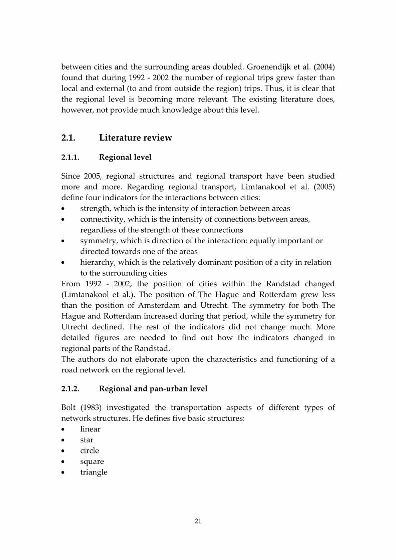
region
city or pan‐urban
district or part of a city
neighbourhood
20
A region comprises a main city, a few middle‐sized cities and a number of
villages. The urban areas in a region are usually strongly related to each
other. Regions can have different sizes and different numbers of inhabitants.
The resemblance is in the coherence of the areas in a region. A city is a well‐
defined type of area. Cities can differ very much in size and number of
inhabitants. Still the mechanism of what makes an area to act as a city is
universal. The term ʹpan‐urbanʹ is mostly used to express that all activities of
a completely urbanized area are incorporated: sometimes a few cities are so
close to each other that they are almost like one city. A part of a city or district
is a level at which important components of a city can function on their own,
like a residential area or a central business district. At the level of the
neighbourhood, activities will mostly be of the same nature (working or
housing). However, at this level the influence of the surrounding areas is
noticeable.
Since the regional level and the city level are very important for this study,
these levels should get most of the attention, although the available literature
does not meet this need. More literature can be found regarding the pan‐
urban level, and still more about the district and neighbourhood levels.
Despite these restrictions, each level is described as well as possible.
In many cases, the available information about network structures lacks
relevant data about road safety. So for this reason only network structures
will be discussed of which a link to road safety is known.
Several authors have paid attention to the structure of road networks.
Important systematic explorations regarding characteristics and effects of
different structures were reported in the sixties and seventies by Holroyd
(1966, 1968), Jansen & Bovy (1974a, 1974b, 1975). Later on Bolt (1983),
Vaughan (1987), Wright et al. (1995) and Marshall (2005) increased
knowledge about this subject. These studies rarely focus on the regional
level, however. This level only appears to have become relevant for planning
and design purposes recently. The provinces have their ʹstreekplannenʹ
(regional plans), but these are mainly aimed at making spatial planning
choices (directing functions to areas, like housing, working and recreation).
These plans do not relate to road network structures. The Netherlands does
not have a governmental layer responsible for the regional road network.
The provinces are the road authority of only a few, mostly unconnected,
roads. So the regional network does not have an ʹownerʹ. The importance of
this network level, however, has grown because the number of regional trips
has increased and is still increasing. This was already made clear by Jansen &
Van Vuren (1985) who concluded that the number of internal car trips in a
city declined by thirty percent while, at the same time, the external car trips
21
between cities and the surrounding areas doubled. Groenendijk et al. (2004)
found that during 1992 ‐ 2002 the number of regional trips grew faster than
local and external (to and from outside the region) trips. Thus, it is clear that
the regional level is becoming more relevant. The existing literature does,
however, not provide much knowledge about this level.
2.1. Literature review
2.1.1. Regional level
Since 2005, regional structures and regional transport have been studied
more and more. Regarding regional transport, Limtanakool et al. (2005)
define four indicators for the interactions between cities:
strength, which is the intensity of interaction between areas
connectivity, which is the intensity of connections between areas,
regardless of the strength of these connections
symmetry, which is direction of the interaction: equally important or
directed towards one of the areas
hierarchy, which is the relatively dominant position of a city in relation
to the surrounding cities
From 1992 ‐ 2002, the position of cities within the Randstad changed
(Limtanakool et al.). The position of The Hague and Rotterdam grew less
than the position of Amsterdam and Utrecht. The symmetry for both The
Hague and Rotterdam increased during that period, while the symmetry for
Utrecht declined. The rest of the indicators did not change much. More
detailed figures are needed to find out how the indicators changed in
regional parts of the Randstad.
The authors do not elaborate upon the characteristics and functioning of a
road network on the regional level.
2.1.2. Regional and pan‐urban level
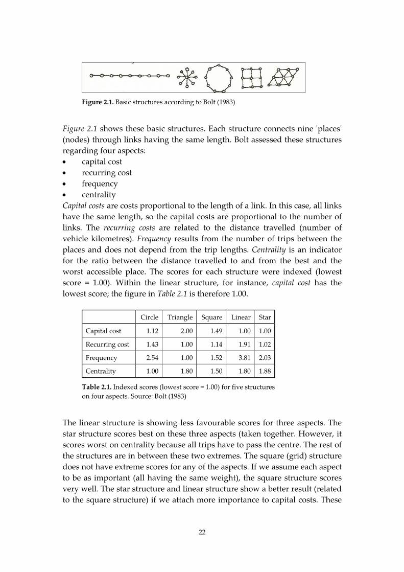
Bolt (1983) investigated the transportation aspects of different types of
network structures. He defines five basic structures:
linear
star
circle
square
triangle
22
Figure 2.1. Basic structures according to Bolt (1983)
Figure 2.1 shows these basic structures. Each structure connects nine ʹplacesʹ
(nodes) through links having the same length. Bolt assessed these structures
regarding four aspects:
capital cost
recurring cost
frequency
centrality
Capital costs are costs proportional to the length of a link. In this case, all links
have the same length, so the capital costs are proportional to the number of
links. The recurring costs are related to the distance travelled (number of
vehicle kilometres). Frequency results from the number of trips between the
places and does not depend from the trip lengths. Centrality is an indicator
for the ratio between the distance travelled to and from the best and the
worst accessible place. The scores for each structure were indexed (lowest
score = 1.00). Within the linear structure, for instance, capital cost has the
lowest score; the figure in Table 2.1 is therefore 1.00.
Circle Triangle Square Linear Star
Capital cost 1.12 2.00 1.49 1.00 1.00
Recurring cost 1.43 1.00 1.14 1.91 1.02
Frequency 2.54 1.00 1.52 3.81 2.03
Centrality 1.00 1.80 1.50 1.80 1.88
Table 2.1. Indexed scores (lowest score = 1.00) for five structures
on four aspects. Source: Bolt (1983)
The linear structure is showing less favourable scores for three aspects. The
star structure scores best on these three aspects (taken together. However, it
scores worst on centrality because all trips have to pass the centre. The rest of
the structures are in between these two extremes. The square (grid) structure
does not have extreme scores for any of the aspects. If we assume each aspect
to be as important (all having the same weight), the square structure scores
very well. The star structure and linear structure show a better result (related
to the square structure) if we attach more importance to capital costs. These
23
two structures keep scoring worse for frequency (related to the square
structure).
2.1.3. Pan‐urban level
Jansen & Bovy (1974b) worked on the issue of the average number of arms of
intersections in a transport network. They used data from six middle‐sized
cities in the Netherlands. For each of the cities the average number appears
to be three arms. Subsequently they checked how many road sections border
a ʹregionʹ (an area having no streets). It appears that on average a ʹregionʹ is
bordered by six road sections. Vaughan (1987) used these results in his
comprehensive study regarding characteristics of road networks and traffic
circulation.
Holroyd (1966, 1968) and Holroyd & Miller (1966) have performed
theoretical analyses to find the effects of different structures (circular and
square structures) on the circulation of traffic. These structures are on a pan‐
urban level. Holroyd uses different combinations of network structures and
routing systems within these structures. His approach was continued and
extended by Vaughan (1987) and Wright et al. (1995).
An important variable used by Vaughan (1987) is the ʹroute factorʹ: dividing
the average distance via the routing system by the average direct distance. A
direct route from origin to destination has a route factor which equals 1. Both
Vaughan and Holroyd (1966) discuss the characteristics of twelve structures
in circular areas; see Figure 2.2.
In each of the twelve areas in Figure 2.2, the same origin‐destination pair is
related to the routing system in that particular area. In three of the structures,
the routing system provides for two alternative routes: external ring / radial,
internal ring / radial, and radial ‐ arc / radial. The author chooses the shortest
one of these two routes.
The lowest average route factor (about 1.1) can be found in structures with
triangular roads as well as in structures with routes through both ring roads
and radial roads. Other structures (radial, external ring, internal ring) have
route factors up to 1.4. The grid and hexagonal structures are in between.
Vaughan does not use the route factor for selecting an optimal structure. He
thinks that traffic distribution is a more important factor to find an optimal
structure. He analyses the given twelve structures regarding traffic volumes,
number of crossing routes and distance travelled. Three structures have a
good score for these factors: radial ‐ arc / radial, radial / arc and rectangular.
The radial ‐ arc / radial structure shows higher traffic volumes in the central
area than the grid structure. However, it shows 17 percent shorter distances
and just as many crossing routes. The radial ‐ arc structure shows almost no
24
traffic in the central area and thirty percent fewer crossing routes than
radial ‐ arc / radial; but the distance travelled is 10 percent longer.
Figure 2.2. Twelve structures in circular areas by Holroyd (1966)
25
In addition, Vaughan (1987) analyzed spiral structures; some of the spiral
structures score very well for the aforementioned factors. Hidber (2001)
considers a spiral structure as a rolled up linear structure: the spiral structure
has the advantages of the linear structure, while at the same time it has a
very compact form. In practice, spiral structures are hardly applied.
Vaughan also analysed the rectangular structures, described by Holroyd
(1968). Holroyd takes a rectangular structure in which housing and working
areas are distributed uniformly and independently. Part of the trips between
home and work will not cross each other, and the other part will cross. The
latter part can be calculated. When all routes would cross, the result equals
to 1, and if crossing does not occur the result equals 0. The theoretical
minimum, calculated by Holroyd (1968) equals 0.125. This means that in a
road network at least one eighth of the trips will cross each other. Holroyd &
Miller (1966) showed that the minimum value is 0.125 in a circular city. In a
rectangular city (Vaughan, 1987; p. 258) this value equals 0.222.
Subsequently Holroyd (1968) calculated the expected number of crossing
routes per pair of routes, given a rectangular structure, when the route choice
is used as an input, e.g. vehicles turn right as much as possible or vehicles
choose a turning point remote from the centre. The results of the calculations
for five routing systems are laid down in Table 2.2. The system with a
random choice has the highest value (0.222). The lowest value is 0.156, which
can be attained by relieving the city centre.
Routing system C
Random choice 0.222
Right‐turning 0.222
East‐west section remote from east‐west axis 0.167
Turning‐point remote from centre (rectangular distance) 0.156
Turning‐point remote from centre (straight‐line distance) 0.156
Table 2.2. The expected number of crossing routes per pair of routes C in a
rectangular structure, varied by routing system. Source: Holroyd (1968)
Vaughan (1987) also examined the possibilities to reduce both the distance
travelled and the number of crossing routes (C). This analysis was applied to
ʹSmeedʹs cityʹ, a theoretical city in which origins and destinations are
uniformly distributed. For this city, different structures were evaluated
regarding distance travelled and crossing routes (Figure 2.3). The circular
structure with radial‐arc (See also Figure 2.2) scores very well, better than the
26
spiral structures. The spiral structures, In their turn, score better than the ring
structures. Vaughan stresses that these results are valid for roads all having
the same characteristics (speed limit, capacity). It is obvious that these results
are very much of a theoretical nature, because both the assumptions for a
Smeedʹs city and the characteristics of the roads can hardly ever be found in
actual practice. One can question whether this method can even be applied to
a real network. It is possible to calculate the values for the distance travelled
and for C in a real network. Subsequently, these values can be compared to
the values of the theoretical structures. If the differences are high, it may be
concluded that the real network needs improvement. This will be further
discussed in Chapter 5.
0.00
0.05
0.10
0.15
0.20
0.25
0.30
0.35
0.0 0.5 1.0 1.5 2.0 2.5
Average distance travelled
C
spiral ring
radial
minimum distanceRg= 0.2
Rg= 0.328
Rg= 0.50Rg= 0.6
Rg= 0.707
Rg= 0.8
Rg= 0.9
minimum crossings
internal ring 10°
radial‐arc/radial30°
60°
radial‐arc
80°direct
minimum possible crossings
minim
um average distance
external ring
Figure 2.3. Mean number of crossings per pair of routes (C) and average distance
travelled (based on data according to Vaughan, 1987; p. 302).
Hidber (2001) also analyses three theoretical structures: a square city with a
grid structure, a circular city with radials and concentric circles, and a purely
linear city. He splits these cities up into zones. The amount of traffic between
the zones depends on four types of resistance: exponential, quadratic, and
linear (inversely proportional to distance), and a type that is independent of
distance (without any resistance). Hidber compares these types with regard
to three criteria:
accessibility (expressed as travel time of distance)
amount of internal traffic (traffic which does not leave its zone)

27
number of vehicle kilometres (sum of the amount of traffic between the
zones times the distance)
The amount of internal traffic depends on the type of resistance.
The linear city appears to have the largest amount of internal traffic (which is
favourable for potential pedestrian trips), lowest accessibility, and a high
number of vehicle kilometres (as compared to the other city types). The
square city as well as the circular city show a uniform distribution of traffic
over the road network.
2.1.4. Pan‐urban, district, neighbourhood
Snellen (2001) investigated relationships between city structure and activity
patterns. The aim was to find whether the city structure could have an
influence on the reduction of the number of car trips. The structures studied
are located at three levels:
pan‐urban: ring, grid, radial
district: ring, loop, radial, axial (a distributor connected to a main road),
grid, tangential
neighbourhood: loop/tree, loop, loop/grid, grid, tree
The influence of the urban form on travel patterns (concerning daily
activities) appears to be small. A positive influence of fewer car trips is
related to:
poly nuclear, radial or axial district distributors
neighbourhood distributors by way of loop/tree and loop/grid
The number of car trips is not likely to be reduced in case of:
urban distributors by way of a ring
district distributor by a loop or ring
neighbourhood by loop
A large neighbourhood shopping centre, district sports facilities, a longer
distance to the city centre, situation within the Randstad, and a lower degree
of urbanization of a district do not contribute to car trip reduction either.
2.1.5. Pan‐urban, district
Marshall (2005) reported about an extensive study of characteristics of road
structures and routing systems within these structures. Routing systems or
routing structures have three main properties:
28
depth: the maximum distance to be travelled into an area
continuity: the number of links that a route is made up of, e.g. a route
with four links has a smaller continuity than a route, having the same
length, with two links
connectivity: the number of routes to which a given route connects
These properties can be calculated for each routing system.
2.1.6. Traffic circulation system in general
The circulation system determines the distance travelled and the number of
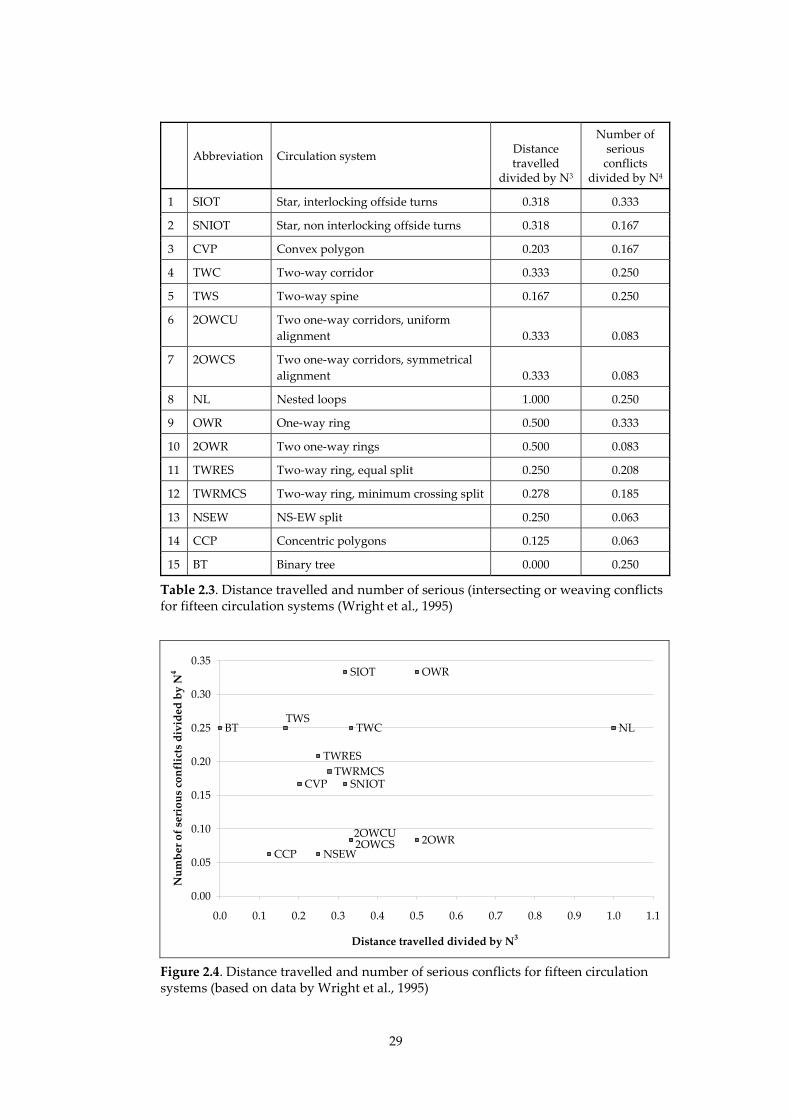
conflicts between vehicles. Wright et al. (1995) investigated fifteen circulation
systems (see Appendix A for a description) with N nodes (having both origins
and destinations). For each system they calculated the distance travelled and
the number of conflicts (C) (assuming N is very large). The conflicts consist of
four types: intersecting, weaving, merging, diverging and shunting (rear‐
end) conflicts. Of these types, only intersecting and weaving conflicts are
serious conflicts. Table 2.3 shows the distance travelled and the number of
serious conflicts for each of the fifteen circulation systems. The same
variables are shown in Figure 2.4.
The systems at the bottom left hand side of Figure 2.4 have favourable scores on
both variables: the number of serious conflicts is relatively low and so is the
distance travelled. Wright et al. (1995) stress the relevance of more variables
when choosing a circulation system:
adaptability: the system should have to fit existing structures on all
levels
robustness: the system should be able to handle the transport demand
simplicity: simple systems are easier to understand
compliance: drivers should be easily routed through the system
Systems 2OWCU, 2OWCS, NL, 2OWR and NSEW are not very robust.
Systems 2OWCU, 2OWCS and NL can be applied within closed systems like
conveyor systems in factories. Systems SIOT, SNIOT, TWC, TWS, OWR,
2OWR, TWRES, TWRMCS and BT can be implemented in both rectangular
grids and ring‐radial networks. Systems NSEW and CCP need a large road
length.
29
Abbreviation Circulation system Distance travelled
divided by N3
Number of serious conflicts
divided by N4
1 SIOT Star, interlocking offside turns 0.318 0.333
2 SNIOT Star, non interlocking offside turns 0.318 0.167
3 CVP Convex polygon 0.203 0.167
4 TWC Two‐way corridor 0.333 0.250
5 TWS Two‐way spine 0.167 0.250
6 2OWCU Two one‐way corridors, uniform
alignment 0.333 0.083
7 2OWCS Two one‐way corridors, symmetrical
alignment 0.333 0.083
8 NL Nested loops 1.000 0.250
9 OWR One‐way ring 0.500 0.333
10 2OWR Two one‐way rings 0.500 0.083
11 TWRES Two‐way ring, equal split 0.250 0.208
12 TWRMCS Two‐way ring, minimum crossing split 0.278 0.185
13 NSEW NS‐EW split 0.250 0.063
14 CCP Concentric polygons 0.125 0.063
15 BT Binary tree 0.000 0.250
Table 2.3. Distance travelled and number of serious (intersecting or weaving conflicts for fifteen circulation systems (Wright et al., 1995)
SNIOTCVP
TWC NL
OWR
2OWR
TWRES
TWRMCS
NSEWCCP
BT
SIOT
TWS
2OWCU2OWCS
0.00
0.05
0.10
0.15
0.20
0.25
0.30
0.35
0.0 0.1 0.2 0.3 0.4 0.5 0.6 0.7 0.8 0.9 1.0 1.1
Distance travelled divided by N3
Number of serious conflicts divided by N
4
Figure 2.4. Distance travelled and number of serious conflicts for fifteen circulation systems (based on data by Wright et al., 1995)
30
2.2. Criteria for evaluating (road) networks
The findings from literature provide good suggestions for evaluating road
networks, routing systems and circulation system. They make clear which
kind of characteristics, classifications, variables and criteria can be used for a
proper evaluation. The most important criteria are listed below.
Routing systems and distribution systems
depth: the maximum distance to be travelled into an area
continuity: the number of links that a route is made up of, e.g. a route
with four links has a smaller continuity than a route, having the same
length, with two links
connectivity: the number of routes to which a given route connects
strength, which is the intensity of interaction between areas
symmetry, which is the direction of the interaction: equally important
or directed towards one of the areas
hierarchy, which is the relatively dominant position of a city related to
the surrounding cities
traffic circulation system: limitations in driving directions, routing
through the central area
number of crossing vehicles: frequency of crossing
number of serious conflicts: type of conflicts (intersecting, weaving,
merging, diverging, rear‐end)
Road networks and road structures
type of structure on different levels
total length of all links: road length
number of intersections
average number of arms of intersections
traffic volumes: road section level or network level
adaptability: the system should have to fit existing structures on all
levels
robustness: the system should be able to handle the transport demand
simplicity: simple systems are easier to understand
compliance: drivers should be easily routed through the system
31
2.3. Summary
A great variety of indicators and variables is available for describing,
analyzing, and evaluating routing systems, distribution systems, road
networks and road structures. Several authors have applied these indicators
and variables to a great number of structures and systems, often on a
theoretical basis, sometimes using data from actual practice.
Indicators based on the number of crossing or conflicting vehicles and the
type of these conflicts are relevant if road structures need to be selected for
attaining more road safety. Literature shows a number of indications about
some road structures having a low number of crossing vehicles. On the other
hand, these structures may result in larger distances travelled, which means
more exposition to risk. In theory, some structures have a low number of
crossings as well as small distances travelled. Wright et al. (1995) find this
property for convex and concentric polygons, ʹtwo one‐way corridorsʹ and a
North/South ‐ East/West split. Vaughan (1987) and Holroyd (1968) find this
for circular structures with routing systems radial‐arc/radial, radial/arc and
rectangular. They also find rectangular structures with a routing system in
which vehicles make turning movements remote from the centre, in order to
relieve the city centre. These structures deserve more attention from
researchers. In these kinds of structures, all roads are more or less of the
same class (no hierarchy, same design). Adding a classification system will
change the results mentioned above.
32
3. Road network structure and road classification
Road classification is meaningful for both road authorities and road users.
The road authority needs road classification for an efficient use of the road
network and for setting priorities in allocating its budgets. The coherence of
the road classes within a network, the road network structure, is also
relevant for road classification. Network structure and road classification can
assist the road user in choosing a safe and quick route. A characteristic
design of a road class will also help the road user to be aware of the
behaviour expected of him/her (recognisability), which other types of road
users can be expected on the road, and what sort of behaviour can be
expected from those other road users (predictability). To stimulate
recognisability and predictability each road class needs its own characteristic
design elements. Research on which elements are to be used is continuing. In
addition, some design elements are required for enlarging the safety level of
a road class, by regulating speed differentials and by mixing or separating
different types of road users.
It is easier to change or adapt the road classification selected than it is to
change the road structure. For example, putting up a road sign may be
sufficient to change the (formal) road class. In principle, however, road
classification comprises much more than the mere placement of road signs.
Roads should be designed and all appropriate design elements should be
introduced according to road class requirements. Road classes should be
relatively positioned in the road network structure in order to optimize
safety, flow and accessibility.
3.1. Functionality of roads
3.1.1. Network structure
Determining the functionality of roads and of the road network, i.e. the
network structure, precedes road classification. The network structure is
dependent on the trips taken in an area and its surrounding areas. Trips are
dependent on the size of these areas, and on the nature of the trip (home ‐
work, home ‐ shop etc.). Connections between areas will facilitate trip‐taking.
The capacity of these connections needs to be tuned to the expected traffic
volumes. A connection designed for high motor vehicle volumes can only be
built at high costs. Planning these kinds of connections requires much
33
attention to assure that the investments are used for the right purpose, and
will be cost‐effective. When planning a network structure, each type of
connection is put into place. Subsequently, road classification adds factors to
functionality regarding the road environment as well as the presence of
different types of road users.
3.1.2. Roads and environmental areas
A good example of network structure in urban areas is the division in two
types of areas: (main) roads and environmental areas (Minister of Transport,
1963; Goudappel & Perlot, 1965).
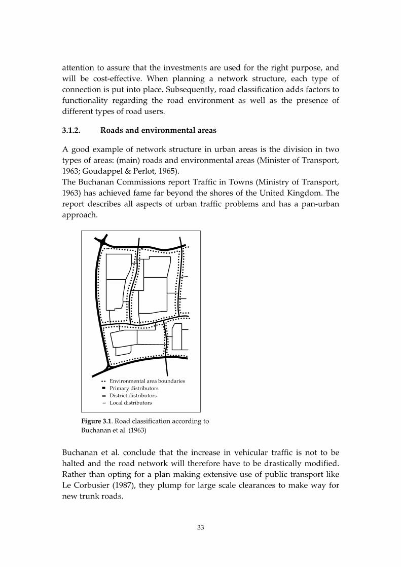
The Buchanan Commissions report Traffic in Towns (Ministry of Transport,
1963) has achieved fame far beyond the shores of the United Kingdom. The
report describes all aspects of urban traffic problems and has a pan‐urban
approach.
Figure 3.1. Road classification according to
Buchanan et al. (1963)
Buchanan et al. conclude that the increase in vehicular traffic is not to be
halted and the road network will therefore have to be drastically modified.
Rather than opting for a plan making extensive use of public transport like
Le Corbusier (1987), they plump for large scale clearances to make way for
new trunk roads.
Environmental area boundaries
Primary distributors
District distributors
Local distributors
34
Buchanan et al. also include so‐called environmental areas in their plan, to
take on the functions of the lower‐traffic residential area (Figure 3.1). These
environmental areas may not be too large lest the number of vehicles exceeds
the environmental capacity. This is defined in the simplest of terms, the main
criterion being the ease with which a street in the area can be crossed. This
ʹpedestrian delayʹ factor is however variable according to the number of
vulnerable pedestrians (old people, children: the level of vulnerability) and
the degree to which a street can be read, i.e. the degree to which the situation
in the street can be seen at a glance: (parked cars, number of obscured exits,
driveways etc.: the level of protection). This approach means that, for
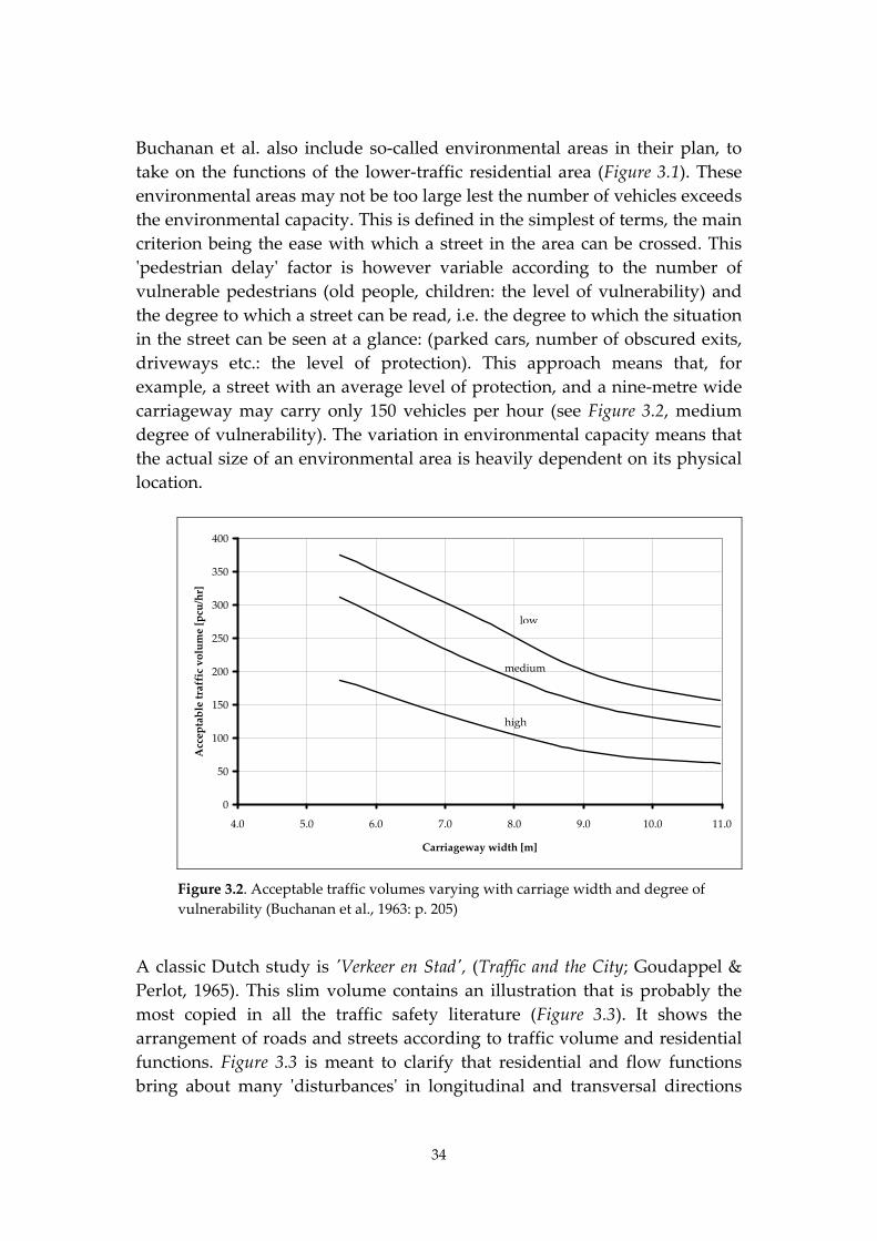
example, a street with an average level of protection, and a nine‐metre wide
carriageway may carry only 150 vehicles per hour (see Figure 3.2, medium
degree of vulnerability). The variation in environmental capacity means that
the actual size of an environmental area is heavily dependent on its physical
location.
0
50
100
150
200
250
300
350
400
4.0 5.0 6.0 7.0 8.0 9.0 10.0 11.0
Carriageway width [m]
Acceptable traffic volume [pcu/hr]
low
high
medium
Figure 3.2. Acceptable traffic volumes varying with carriage width and degree of
vulnerability (Buchanan et al., 1963: p. 205)
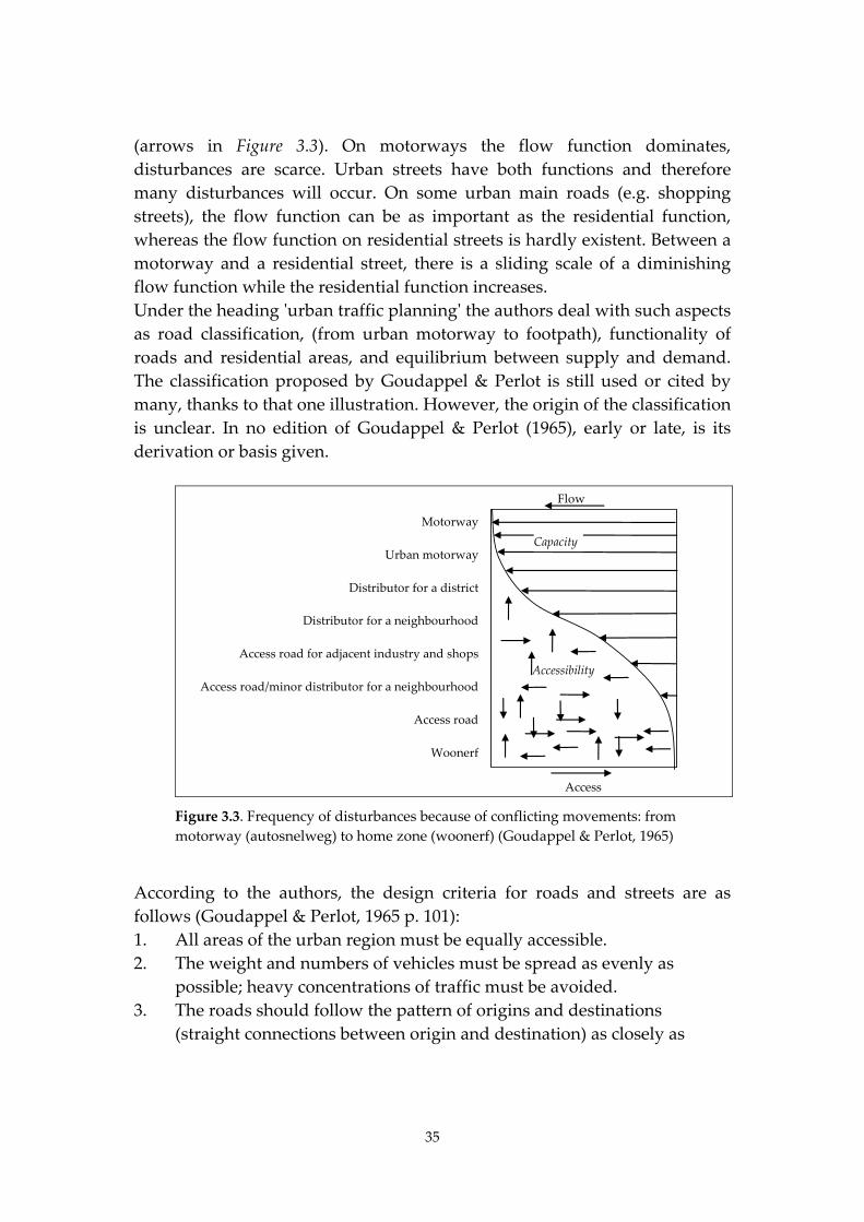
A classic Dutch study is ʹVerkeer en Stadʹ, (Traffic and the City; Goudappel &
Perlot, 1965). This slim volume contains an illustration that is probably the
most copied in all the traffic safety literature (Figure 3.3). It shows the
arrangement of roads and streets according to traffic volume and residential
functions. Figure 3.3 is meant to clarify that residential and flow functions
bring about many ʹdisturbancesʹ in longitudinal and transversal directions
35
(arrows in Figure 3.3). On motorways the flow function dominates,
disturbances are scarce. Urban streets have both functions and therefore
many disturbances will occur. On some urban main roads (e.g. shopping
streets), the flow function can be as important as the residential function,
whereas the flow function on residential streets is hardly existent. Between a
motorway and a residential street, there is a sliding scale of a diminishing
flow function while the residential function increases.
Under the heading ʹurban traffic planningʹ the authors deal with such aspects
as road classification, (from urban motorway to footpath), functionality of
roads and residential areas, and equilibrium between supply and demand.
The classification proposed by Goudappel & Perlot is still used or cited by
many, thanks to that one illustration. However, the origin of the classification
is unclear. In no edition of Goudappel & Perlot (1965), early or late, is its
derivation or basis given.
Motorway
Urban motorway
Distributor for a district
Distributor for a neighbourhood
Access road for adjacent industry and shops
Access road/minor distributor for a neighbourhood
Access road
Woonerf
Capacity
Accessibility
Access
Flow
Figure 3.3. Frequency of disturbances because of conflicting movements: from
motorway (autosnelweg) to home zone (woonerf) (Goudappel & Perlot, 1965)
According to the authors, the design criteria for roads and streets are as
follows (Goudappel & Perlot, 1965 p. 101):
1. All areas of the urban region must be equally accessible.
2. The weight and numbers of vehicles must be spread as evenly as
possible; heavy concentrations of traffic must be avoided.
3. The roads should follow the pattern of origins and destinations
(straight connections between origin and destination) as closely as
36
possible whereby traffic movement through areas not being part of a
given route is avoided.
4. By ensuring that roads and junctions are of appropriate dimensions, a
fluent and constant traffic flow should be made possible. Road
classification is an important aid to this.
5. In considering future situations, special attention should be paid to
achieving less traffic within an area, with the emphasis on time, rather
than on distance.
Out of three possible traffic systems ‐ radial, tangential (grid) and other,
Goudappel & Perlot opt for the tangential system, with special regard to
criterion 2. For inner cities, they prefer the ring or loop. The authors further
lay down requirements for the positioning of housing. Houses must be easily
accessible on the one hand and must be on a street primarily residential in
nature on the other hand.
At the time of the publication of their report (the sixties) the authors
propagated to tackle traffic problems at the pan‐urban level. Obviously, they
were very much influenced by Buchanan et al.
3.1.3. Mesh
Van Minnen & Slop (1994) proposed a mesh of 10 km for distributors in rural
areas. In that case the travel time from an origin to the nearest distributor
would take 3 to 5 minutes at the most for 90 percent of the trips. This
proposal was not adopted by CROW (1997). However, CROW did not offer
any alternative. Therefore, the network structure of rural roads did not get a
quantitative criterion regarding the mesh.
For urban residential areas, Van Minnen (1999) concludes that the size,
varying from 65 to 80 ha (900 times 900 m2 at the most), comes up to
expectations. Criteria for his evaluation were trip length (within and outside
the area), traffic volumes within the area, percentage of through‐traffic,
driving speeds of motorized vehicles, accessibility of facilities, and
accessibility to public transport and to emergency services. In addition, the
pedestrian delay factor was evaluated. Most of these criteria were evaluated
by means of simple calculations as well as by data based on experiences from
recently installed zone 30 areas.
In the former Swedish guidelines for network structure of urban roads
(SCAFT, 1968), regional distributors have a mesh of 2,500 m, district
distributors a mesh of at least 1,000 m and local distributors a mesh of at least
250 m. These values were primarily chosen from a safety point of view. A
number of considerations were taken into account:
37
sufficient space for entries and exits
drivers should be able to anticipate the next intersection
overtaking should be possible
In addition, hands‐on experience played a role in choosing the mesh values.
In more recent publications (TRÅD, 1982; SALA, 1999) the mesh values were
not used anymore.
Ewing (2000) analysed a theoretical design of a road network, using the
following variables:
number of dwellings per area
number of car trips per dwelling per day
average trip length
share of rush hour traffic
capacity of a road (in number of vehicles per lane per hour)
main roads with a maximum of four lanes, distributors with a
maximum of two lanes (both road types are part of a grid)
The number of dwellings per area varies from 2.5 per ha to 124 per ha. The
mesh of the main roads varies accordingly from 4,000 m to 81 m; in all cases,
there is one distributor in between each pair of main roads. After the
introduction of an elasticity factor the mesh becomes bigger for the high
dwelling densities (from 81 m to 145 m). Subsequently, peak spreading is
introduced as well as an adaptation of road capacity. Finally, the mesh for
main roads becomes 3.107 m for low dwelling densities and 111 m for high
dwelling densities (Table 3.1).
Density of
dwellings
(dwellings/ha)
Vehicle
kilometres
(mvhkm/km²/h)
One‐way or
two‐way
traffic
Mesh of
main roads
(m)
Mesh of
distributors
(m)
2.5 2,580 2 3,107 1,546
9.9 6,775 2 1,121 560
17.3 10,397 2 663 332
24.7 13,424 2 444 222
37.0 17,380 2 188 93
49.4 21,948 1 280 140
74.1 30,979 1 171 85
123.5 47,823 1 111 55
Table 3.1. Mesh values at varying dwelling densities adjusted for peak spreading
and road capacity. From Ewing (2000)
38
The mesh values calculated by Ewing differ from the proposed values by
SCAFT (1968). Ewing mainly assumes variations in the dwelling density,
while SCAFT focuses on safety criteria regarding minimum lengths of road
needed for drivers to anticipate and to overtake. SCAFT does not take the
dwelling density into consideration.
3.1.4. Network structure through spatial distribution of (housing)
clusters
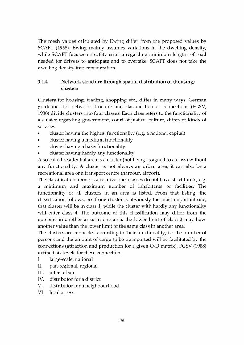
Clusters for housing, trading, shopping etc., differ in many ways. German
guidelines for network structure and classification of connections (FGSV,
1988) divide clusters into four classes. Each class refers to the functionality of
a cluster regarding government, court of justice, culture, different kinds of
services:
cluster having the highest functionality (e.g. a national capital)
cluster having a medium functionality
cluster having a basis functionality
cluster having hardly any functionality
A so‐called residential area is a cluster (not being assigned to a class) without
any functionality. A cluster is not always an urban area; it can also be a
recreational area or a transport centre (harbour, airport).
The classification above is a relative one: classes do not have strict limits, e.g.
a minimum and maximum number of inhabitants or facilities. The
functionality of all clusters in an area is listed. From that listing, the
classification follows. So if one cluster is obviously the most important one,
that cluster will be in class 1, while the cluster with hardly any functionality
will enter class 4. The outcome of this classification may differ from the
outcome in another area: in one area, the lower limit of class 2 may have
another value than the lower limit of the same class in another area.
The clusters are connected according to their functionality, i.e. the number of
persons and the amount of cargo to be transported will be facilitated by the
connections (attraction and production for a given O‐D matrix). FGSV (1988)
defined six levels for these connections:
I. large‐scale, national
II. pan‐regional, regional
III. inter‐urban
IV. distributor for a district
V. distributor for a neighbourhood
VI. local access
39
Figure 3.4 shows how clusters are connected. Similar classes have a direct
connection, while clusters of different classes are connected by two
connections not belonging to the same level, thus creating a hierarchy in
connecting clusters.
large‐scale, national
pan‐regional, regional
inter‐urban
distributor, district
distributor, neighbourhood
local access
highest functionality medium functionality low functionality hardly any functionality residential area
C3
C5
C1
C2
C4
C1
C2
C3
C4
C5 C5
C4
C3
C2
C1
Figure 3.4. System of connections between cluster types
The 1988 guidelines (Leitfaden für die funktionale Gliederung des
Straßennetzes RAS‐N) were recently replaced by newer guidelines
(Richtlinien für integrierte Netzgestaltung RIN) (FGSV, 2008). Gerlach (2007)
provides an overview of the differences between the old and new guidelines.
The classification of clusters with characteristic functionality remains.
However, an additional functionality was added: the metropolis (read as
Berlin). The number of connections remains six, but their nature is somewhat
different. The lowest level IV disappears, and a new highest level is
introduced: the continental connection (between countries). The numbering
starts at level ʹ0ʹ and ends at level V.
RAS‐N only applied to motorized traffic (in particular private cars), RIN also
deals with public transport and bicycle traffic. RAS‐N did not indicate a
preference for the level of accessibility of clusters, in terms of intended travel

40
times for different types of connections. RIN does give these indications of
travel time in minutes. Travelling by car to a cluster C3 should not take
longer than 20 minutes, to a cluster C2 30 minutes, and to a cluster C1 60
minutes. Between two C3 clusters, the maximum travel time should be 25
minutes, between two C2 clusters 45 minutes and between two C1 clusters
180 minutes.
3.1.5. Road classification
The North American ʹBlue Bookʹ presented a road classification system for
rural roads (in 1954); the first of this kind of classification systems. Weiner
(2008) gives an overview of the development of the classification systems in
the United States. Janssen (1974) proposed a road classification system that
would contribute, at least theoretically, to more road safety. The formal road
classification in the Netherlands was established by RONA (1992). Janssen
(1991a) set up a road classification for urban roads; this system was not
accepted however. Finally, a road classification system for all road types was
introduced (CROW, 1997) according to the principles of Sustainable Safety
(Koornstra et al., 1992). Infopunt DV (1999, 2000) elaborated this
classification, particularly the design elements within road classes.
According to Janssen (1974), the aim of road classification is to relieve
(simplify) the driving task is. Therefore, the ʹrecognisabilityʹ1) for road users
should be enlarged. Road classification should meet the following
requirements:
within a class: consistency, continuity and little variation (uniformity)
in design elements
between classes: clear differences between design elements of each class
number of classes: a limited number
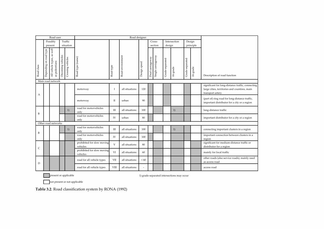
RONA (1992) uses a classification system with four main classes for roads
outside urban areas (rural areas); see Table 3.2. Each main class is divided up
into two classes. One of these classes is taken as the standard class, the other
one is a sub‐standard class.
RONAʹs main classes are characterized by the number of carriageways, by
the design speed, and by the types of intersections. Janssen (1988, 2005)
shows the differences between these classes regarding their risk (number of
crashes divided by the number of motor vehicle kilometres); see Table 3.3.
1) The driver is easily able to understand which road type he is driving on.
Depending on road type
All vehicle types, as well
as ped
estrians
Oncoming vehicles
Crossing vehicles
Dual carriagew
ay
Single carriagew
ay
Grade‐separated
At‐grade
Grade‐separated
At‐grade
motorway I all situations 120
significant for long‐distance traffic, connecting
large cities, territories and countires, main
transport artery
motorway II urban 90(part of) ring road for long‐distance traffic,
important distributor for a city or a region
1)road for motorvehicles
onlyIII all situations 100 1) long‐distance traffic
road for motorvehicles
onlyIV urban 80 important distributor for a city or a region
1)road for motorvehicles
onlyIII all situations 100 1) connecting important clusters in a region
road for motorvehicles
onlyIV all situations 100
important connection between clusters in a
region
prohibited for slow moving
vehicles V all situations 80
significant for medium‐distance traffic or
distributor for a region
prohibited for slow moving
vehicles VI all situations 60 mainly for local traffic
road for all vehicle types VII all situations < 60other roads (also service roads), mainly used
as access road
road for all vehicle types VIII all situations ‐ access road
present or applicable 1) grade‐separated intersections may occur
not present or not applicable
Road designer
C
Road user
Possibly
present
Traffic
situation
Road class
Cross‐
section
Intersection
design
Design
principle
Road type (nam
e)
A
B
Main road network
Road type
Road environment
Description of road function
B
D
Other road networks
Design speed
Table 3.2. Road classification system by RONA (1992)
42
Year
Road class 1986 1998
Autosnelweg (motorway) 0.07 0.06
Autoweg (road only for fast motor vehicles) 0.11 0.08
Weg met geslotenverklaring
(road on which slow moving vehicles are not allowed)
0.30 0.22
Weg voor alle verkeer (road for all traffic) 0.64 0.43
Outside urban
areas
(rural area)
Sum rural area 0.23 0.16
Verkeersader (main road) 1.33 1.10
Woonstraat (residential street) 0.74 0.57
Urban area
Sum urban area 1.16 0.94
All road types 0.53 0.35
Table 3.3. Key safety indicators for rural RONA road classes and for urban road classes
(adaptation by the author of Janssen, 1988 and 2005)
These differences appear to be quite large, the risk increases with the number
of disturbances (from motorway to road for all traffic, and from residential
street to main road). Many disturbances occur when through traffic mixes
with local traffic, when slow moving vehicles mix with motor vehicles, when
pedestrians cross a street, and when many vehicles overtake others on a road
with a single carriageway.
The introduction of Sustainable Safety resulted in a new road classification
system (Janssen, 1997; CROW, 1997):
fewer road classes: three instead of eight classes in rural areas
mono‐functionality of each road class: a class is either intended for
flowing or for offering access, in between there is a road class which
connects the other two classes
potentially serious conflicts are not allowed: e.g. frontal conflicts (on 80
kph roads) are prevented by separating (physically) vehicles driving in
opposite directions
ʹessentialʹ characteristics should enhance recognisability: number of
carriageways, presence of an emergency lane, longitudinal marking
In urban areas road classification is a matter of splitting the area up into
residential areas (access roads, preferably grouped within a zone 30) and
areas for main roads (distributor roads).

43
3.2. Homogeneity of traffic within a road class
The term homogeneity comprises all available means:
to restrict the differences in speeds, driving directions and masses
to separate types of road users, in particular pedestrians and cyclist
from motorized traffic
to lower speeds if the previous means are either not present or not
preferred
Several traffic measures are available for improving homogeneity. A physical
separation is meant to prevent differences in driving directions, one lane for
each direction will reduce driving speeds, bicycle paths and lanes will
separate cyclists from motorized traffic, a roundabout will decrease speeds
and reduce the number of serious conflicts at intersections, and a hump will
reduce speeds at road sections. These kinds of traffic measures will most
probably reduce the number of crashes, as is shown by Dijkstra (2003).
Guidelines (CROW, 1997) and recommendations (Infopunt DV, 1999 and
2000) were formulated to establish a specific set of design elements for each
road class. Doumen & Weijermars (2009) conclude that the implementation
of these guidelines and recommendations is still in progress.
Design elements that stimulate recognisability as well as predictability
Janssen (1974) states: ʺA road class will function efficiently if the road
characteristics create the right expectations to the road user regarding his
traffic behaviour (choice of route and manoeuvres) and the behaviour of the
other road users.ʺ The term ʹexpectationsʹ is too inexact to use in research.
That is why mostly characteristics have been studied which drivers use when
classifying roads (Noordzij, 1996). Other types of studies used human test
subjects who were shown pictures of road images after which they had to tell
which kind of behaviour would be appropriate (stated preference). In
addition, human test subjects in a simulator were asked to respond to
simulated traffic situations (Noordzij, 1996). Noordzij concludes that human
test subjects who classify roads (usually by sorting photographs), mostly take
the number of carriageways and the number of lanes as a clue. On the basis
of recent simulator studies, Aarts & Davidse (2007) conclude that a more
recognisable design (according to the design elements of Sustainable Safety)
results in a safer behaviour: lower speeds and a position in the cross‐section
closer to the edge of the road than on the classic road types. However, the
homogeneity of speeds did not improve.
44
3.3. Summary
The Germans have more than forty years of experience in structuring their
road network. Sweden introduced a network structure (for urban areas)
many years ago. And in the Netherlands, the network structure is not a
foregone conclusion. The mesh of main roads in Dutch urban areas was
clarified to some extent; the foundation is the result of a simulation study.
Road classification was introduced at an early stage of the large‐scale car
mobility. On the one hand, road classification is a way of planning and
designing the different functions of roads, on the other hand it helps road
users to make safe and quick trips. For a road authority, road classification is
not necessarily the same as road classification for a road user. The road
authority needs a classification relevant for the road functions and for the use
of the road (as the authority would like it to be). This classification of the
road authority results in a design for each road. The design, amongst other
things, is a prerequisite for homogeneity within road classes. The road user
on the other hand should be able to understand from the road characteristics
and from actual traffic situations (recognisability) how to behave and what
behaviour is to be expected from other road users (predictability). Road
classification should assist the road user in this driving task. This assumption
could be confirmed to some extent.
Road classification is meant to reconcile the aims of the road authority and
the aims of the road user. In Sustainable Safety this reconciliation is included
as the principles of recognisability/predictability and functional‐
ity/homogeneity.
The methods described above, to come to a network structure and to a road
classification are typical methods of network design. The design principles
and rules of thumb are mostly based on hands‐on experience. The scientific
foundation for this set of principles, requirements and rules is very frail.
However, road classification is relevant to this study. To overcome the
frailties in the existing methods, a new method will be described for
classifying roads (Chapter 9). This method is partly based on the German
guidelines.
45
4. Route choice in road networks
In the present study, route choice in road networks is a very important issue;
in this chapter, only the existing knowledge will play a role. The research
carried out in this respect will be explained in Chapter 6.
Studying the use of roads network could be limited to analysing the volumes
of road sections for different periods. However, another type of information
is required in order to find differences between the intended use and the
actual use of roads and road classes. Therefore, a more relevant analysis unit
will be the route: all road sections and intersections between origin and
destination. Analysing a route will show whether the sequence of road
categories meets the requirements of Sustainable Safety. Routes not fitting
these requirements should be adapted or traffic should be advised not to use
those routes.
Several measures are available for these purposes: roadside message signs,
navigation systems, road closures. Their effects are only partially known,
more knowledge is needed, particularly for routes on the regional level.
This chapter also deals with the question: what are the direct effects of route
choice on road safety and what is the nature and size of these effects?
4.1. Route choice as part of Sustainable Safety
A Sustainably Safe traffic system comprises a set of requirements for road
networks. For route choice, the most important requirement is whether the
safest route coincides with the fastest route. Meeting this requirement could
result in car traffic moving through residential areas because:
residential areas are very safe
routes through the areas are mostly short‐cuts
That is why an additional requirement is set:
a residential area may only be the origin or destination of a route
the major part of the route should follow main roads (flow function)
a minor part of the route may follow a distributor
To come to a route choice like this, the resistance (i.e. travel time) of a route
through a residential area must be larger than a route along main roads and
distributors. In addition, the route choice may be influenced by instructions
at the roadside or within a vehicle, and possibly by the design of the road
and its environment. A road network can only be sustainably safe if the
traffic on the main roads keeps flowing. If not the resistance of the residential
46
areas for through traffic will be relatively lower than the resistance of the
main roads.
Another important issue for a sustainably safe road network is road
classification. The classification should correspond to the actual traffic
circulation. This relates to the mesh of the distributor roads and main roads.
Sustainable Safety (CROW, 1997) does not prescribe certain mesh values.
Initially, the so‐called travel time criterion (Van Minnen & Slop, 1994) was
formulated. A driver, starting in a residential area, should reach a distributor
with a few minutes. Drivers only need to be subjected to a low speed limit
for a short while. This criterion sets a limit to the size of residential areas.
Since the criterion could not be based on knowledge yet, the guidelines for
road classification (CROW, 1997) do not encompass it. On the contrary, the
guidelines require residential areas to be ʹas large as possibleʹ. This
requirement will influence the mesh value. In actual practice, this value (in
urban areas) mostly varies from 20 ha to 100 ha (Van Minnen, 1999;
Krabbenbos et al., 2002).
4.2. Route choice in general
The previous Section 4.1 treated route choice from a safety point of view. The
network structure, the mesh of main roads, the relative resistance of routes,
information provided to drivers, are all means to let drivers choose the
routes favourable to both safety and accessibility. In this section, the
background of route choice is discussed. Many authors have studied route
choice. The focus will be on the following questions:
What are the reasons for choosing a route (how and why)?
Which variables will affect route choice?
How are these variables related to each other?
Literature shows that many researchers have been working on these
questions and issues, as the following overview will confirm.
What are the reasons for choosing a route?
Much elementary knowledge about route choice can be found in a study
written by Bovy & Stern (1990). In their view, route choice is part of travel
behaviour, and subsequently travel behaviour is part of spatial behaviour.
Spatial behaviour is the result of ʺa mixture of cognitive and affective
attitudes, emotions, perceptions, cognition and learningʺ (Bovy & Stern, 1990;
p. 25). According to the authors, what is important to spatial behaviour is
that a person will develop decision rules in order to make spatial choices.
47
Successive spatial choices of individuals and groups will result in
behavioural processes that will finally determine spatial structure.
Travel behaviour stems from the series objective situation, personal
perception, subjective situation, and personal decision. Four groups of
factors influence this decision: physical environment, socio‐demographic
environment, normative environment and personal environment (Bovy &
Stern, 1990). Personal environment filters the other three environments.
Route choice is an inseparable part of travel behaviour. The traveller, given
his personal environment, will have to make a choice from the possibilities
offered by the physical environment. A large number of alternative routes
are potentially at his disposal. However, the traveller is not aware of all
alternatives (cognition). His experience is relevant for this cognition. Not all
of the available alternatives are useful for the intended trip, because of
conditions regarding travel time and destination(s). Finally, the traveller
makes a choice by weighing his own preferences as well as the physical
aspects of the alternatives. During a trip new choices sometimes appear, by
additional information about the alternatives for the rest of the trip.
These general notions about route choice will be elaborated below, using
information from literature:
1. What is the structure of the underlying decision processes?
2. Which variables will affect route choice?
3. In which context are these variables valid (temporal and spatial)?
4. How do drivers receive traffic information? And does this information
influence their route choice?
5. Which subdivision of the driver population is relevant?
6. What is the size of the effect?
Influencing route choice by navigation systems will be discussed separately
(Section 4.3).
4.2.1. What is the structure of the underlying decision processes?
Andan & Faivre dʹArchier (2001) have studied how car drivers choose their
routes. The routes were part of regional trips, having a length of 50 to 200
km. The researchers prepared three scenarios, possibly resulting in a route
change. A group of 30 car drivers taking these types of trips was selected.
The drivers were confronted with three scenarios:
adverse weather conditions: varying in seriousness
traffic congestion: either starting at one third or at two thirds of the
route length
re‐routing: a road closure at one third or at two thirds of the route
length
48
Different strategies were stated to adapt route choice behaviour. In the first
scenario, for example, three strategies were found:
staying on the same route; relying on own skills
reducing risk by changing routes or choosing another time of departure
reducing risk by postponing the trip or letting a (more experienced)
passenger drive
Relevant factors for route choice are dependent on the underlying decision
process. The factors for the decision are:
perception of the nature of the disruption
possibilities to react
skills to evaluate the risks
Contributing factors are:
preferences of the driver
skills and knowledge
available resources: e.g. a map, a mobile phone
conditions: time pressure, additional costs
The variability of route choice behaviour is smaller (or the adaptation is more
stable) in the re‐routing scenario compared to the other ones. Car drivers
reacted in two ways.
1. Individual factors (attitude towards dealing with the altered situation,
personal skills, preferences and knowledge) determine their choice,
independent of the nature of the altered situation. Sometimes an
adaptation is inevitable because of the circumstances.
2. A combination of both individual factors and circumstances determine
their choice. This means that, when analysing route choice, both
circumstances and individual factors should be considered.
Conclusions
Quite a few car drivers make reasoned choices, by weighing the risks (of not
adapting) and the advantages (of adapting). Personal preferences are less
important than was assumed. What is also relevant is the context of the trip
and the nature of the disturbances. Drivers are strongly motivated to get as
much relevant information as possible. Some drivers deliberately choose
motorways because up‐to‐date information is mostly provided on this type
of road.
49
4.2.2. Which variables affect route choice?
Wachs (1967) interviewed several hundred car drivers about their route
choices. They preferred routes having a small number of crossroads and
driveways, minor congestion, less stress for the driver, more safety, and the
shortest travel time. They preferred routes along commercial areas or, by
contrast, routes along attractive scenery.
Ueberschaer (1969, 1971) describes an extensive questionnaire survey among
13,000 car drivers. He finds the following relevant factors for route choice:
fastest route, shortest route, less congestion, well‐designed road. Benshoofʹs
(1970) study confirms these results. The preferences for route choice are, in
descending order: fastest route (82%), less congestion (77%), less traffic than
on alternative routes (71%), shortest route (60%). These preferences are also
mentioned by Vaziri & Lam (1983).
Michaels (1965) made drivers choose between two parallel roads, having the
same length. The one road was a toll road, the other one a rural main road.
The choice for either of these roads depends on road type, driverʹs age, trip
frequency, and (less) tension.
De Palma & Picard (2005) find as an additional variable: the aspired level of
certainty about the expected arrival time (aversion to arrive late).
Goldenbeld et al. (2006) sent a questionnaire to 500 car drivers. They
subsequently found that a driver who often travels to the same destination,
changes routes more often.
A delay of at least 15 minutes induces the driver to choose an alternative
route, and to use traffic information. Li et al. (2005) reported the
characteristics of routes most preferred by drivers. Compared to other routes,
these routes have a shorter length and travel time, have fewer idle stops,
fewer signals at intersections, and have a larger share of motorway length.
Zhang & Levinson (2008) find similar results.
None of the studies mentioned shows road safety to affect route choice in
any significant way.
Conclusions
Travel time and trip length appear to be the most important factors in route
choice. A less congested route is preferred as well as routes with a larger
share of motorway length, less uncertainty about travel time, less tension,
and fewer idle stops. A driver who often travels to the same destination,
changes routes more often. Road safety does not appear to be an important
factor in route choice.

50
4.2.3. In which context are these variables valid (temporal and
spatial)?
Ueberschaer (1969, 1971) shows that the number of selected routes increases
in accordance with trip length: two to three routes are usual given a trip
length of 3 to 9km. The number of alternatives decreases at longer distances.
The number of selected routes in a rural network is smaller than in an urban
network; e.g. in a fringe and suburban area the number is smaller than in a
central business district. The number of routes also depends on the volumes
on the main network. Goldenbeld et al. (2006) studied route choice in an area
sized 10 by 20km. The drivers in this survey could choose between three
alternative routes to their destination. Some parts of the routes coincided.
The majority of the drivers choose a route on the motorway. About 30
percent does not opt for an alternative route. The alternatives mostly consist
of other road types, which in 25% of the cases is a regional main road. Two
out of five drivers prefer a route or alternative route on roads not being main
roads.
Li et al. (2005, 2006) studied trips from home to work. Two out of three
drivers prefer only one route, the other ones use two routes (30%) or three
routes (3%). They also found the share of motorway length on the preferred
route is 54% while the share on the alternative route is 33%.
According to Ueberschaer (1969, 1971) car drivers see travel time and travel
distance as the main reasons for their route choice. However, measurements
of times and distances did not always appear to be consistent with the stated
values. The reasons given by car drivers usually preferring motorways were
more in accordance with actual measurements than reasons given by users of
rural and urban roads. Zhang & Levinson (2008) also find that the observed
trip length differs from the perceived trip length. Ueberschaer concluded
from the answers to Benshoofʹs survey, that either route choice is an
irrational process or car drivers do not ʹmeasureʹ route characteristics
accurately. This conclusion was relevant because, at that time, many traffic
models used travel time as the main criterion for route choice. Benshoof
(1970) suggested introducing a set of criteria, consisting of travel time,
number of stops, traffic volumes in direction of travel, and distance. This set
was also used by Ueberschaer (1969). Li et al. (2006) reported a difference
between car drivers using only one preferred route and drivers using more
routes. For the latter group, travel time, trip length, number of idle stops,
number of trip chaining stops (stops with a specific purpose), and the
variation in travel time exceed these of the group with only one route.
51
Michaels (1965) studied the differences between drivers choosing a rural
main road and the ones choosing a toll road. The appreciation of the toll
road, and the actual use of this road, is higher for drivers travelling both
routes more often (from origin to destination). Measurements of the tension
of the drivers showed 46% lower values for users of the toll road. Wachs
(1967) showed that the preference for a route with less congestion, less
tension, and along pleasant scenery is related to a longer trip length.
More than 50 percent of the respondents to the questionnaire used by Vaziri
& Lam (1983), choose for a reduction in travel time and less congestion for
the morning trip, and only choose for less travel time on the way back. About
30 percent does not opt for a time reduction.
Goldenbeld et al. (2006) show that a car driver prefers short travel times and
trip lengths when making commuter trips and business trips. For other
purposes travel time and trip length are less important; familiarity with a
route is more important.
The quality of urban planning aesthetics makes a route more attractive for all
purposes, according to Zhang & Levinson (2008). Commuter trips and trips
with purposes ʹeventʹ and ʹvisitʹ are related to efficient routes. For these
purposes, drivers choose a route they already know. The knowledge about a
route prior to making a trip, explains route choice better than the perceived
characteristics of a route. While the perceived characteristics explain route
choice better than the objectively observed characteristics. According to the
authors, route choice is, in the first place, a matter of prior knowledge, in the
second place a matter of perceived characteristics, and finally, a matter of
objective characteristics.
Conclusions
The number of selected routes is related to the nature of the environment,
rural or urban, and to the volumes on the main road network. Most car
drivers use two or three alternative routes. Quite a few car drivers choose a
route on the motorway. The preference for the motorway is also sizeable
because of the low tension on this road type.
Car drivers mention travel time and trip length as main factors for their route
choice in commuter trips. Yet, perceived travel time and trip length are not
always in accordance wit observed travel time and trip length. The number
of stops and traffic volumes are related factors for route choice. The road
environment (urban planning aesthetics, scenery) will also influence route
choice. Prior knowledge about a route is of more importance for route choice
than perceived route characteristics, which are in their turn, more important
than objective characteristics.
52
4.2.4. How do drivers receive traffic information? Moreover, does this
information influence their route choice?
Shirazi et al. (1988) interviewed commuters by phone. About 40 percent of
these commuters sometimes change their routes, of which a quarter changes
seldom, and a third often to very often. Congestion is the main motivation
for changing. Indicative for this decision are radio information, experience,
pressure to be in time, information on the Electronic Freeway Signs. Two
thirds often to very often listen to radio information.
Three out of four of commuters obtain traffic information by listening to the
radio before departure (Wenger et al., 1990). However, this information
hardly has any influence on the decisions regarding the trip; travel mode (car
or bus) and departure time are seldom changed. On average commuters
decided to change their route before departure twice a month. Traffic
information during the trip is dominant for changing routes, the observed
traffic situation is of less importance. About a third of the commuters do not
know whether their decision to change the route was right. The majority of
the commuters get feedback about their choice more than five minutes after
making the decision.
Spyridakis et al. (1991) conclude that recent traffic information, observed
congestion, and time of day affect route choice. Time pressure and weather
conditions have a smaller influence on route choice. Commuters actually
changing their routes are influenced by all of these factors. More than half of
the commuters would like to get traffic information before departure; the rest
prefers receiving information just before entering the motorway. Traffic
information sometimes or regularly influences departure time; it sometimes
or regularly influences route choice before departure. The information before
departure is obtained by radio or television. Half of the commuters change
their routes while travelling, because of traffic information received by radio
or electronic message signs. Radio information is most helpful, electronic
message signs are less helpful.
Jou et al. (2005) interviewed car drivers along a motorway. The respondents
mentioned radio, the Internet and variable message signs as a way of getting
up‐to‐date traffic information. A substantial number of drivers (44%) use
these media quite often or every time. One tenth does not take note of this
kind of information.
Goldenbeld et al. (2006) reported that car drivers do not choose their
preferred routes if information is available about a possible queue or if they
can avoid congestion. For one third of the drivers, route choice depends on
traffic information by radio, television or the Internet, prior to departure.
53
Only a small number use navigation systems. Along the way, more than half
of the drivers (59%) use information sources; most of them use the radio or
electronic message signs (DRIPs). Only 3 percent use a navigation systems.
Conclusions
Prior to making a trip, a considerable number of car drivers take note of
traffic information, mostly by radio, television and the Internet. This
information influences the route choice or departure time for only a small
number of drivers. Along the way, traffic information mostly originates from
radio, own observation, electronic message signs, and sometimes from a
navigation system. A substantial number of drivers change routes because of
this information.
4.2.5. Which subdivisions of the driver population are relevant?
Wenger et al. (1990) divided commuters in four clusters, differing in
flexibility regarding departure time, likelihood to change routes after
receiving information before departure, searching for information before
departure, and the level of tension on the preferred route. The four clusters
are:
Route changers (21%), those willing to change their commuting routes
on or before entering the motorway
Non‐changers (23%), those unwilling to change departure times,
transportation modes, or commuting routes
Time and route changers (40%), those willing to change both departure
time and commuting routes
Pre‐trip changers (16%), those willing to make time, mode or route
changes before leaving the house but unwilling to change en route
Conclusions
Commuters can be divided up into clusters differing in flexibility regarding
departure times and levels of tension on the preferred route as well as
likelihood to change routes on account of information along the way or
information prior to departure.
4.2.6. What is (the size of) the effect of traffic information?
Kraan et al. (1999) evaluated the effect of installing seven additional variable
messages signs along the southern part of the Amsterdam ring road
(motorway A10). On this part of the road drivers can choose between two
parallel routes (A10 and A9).
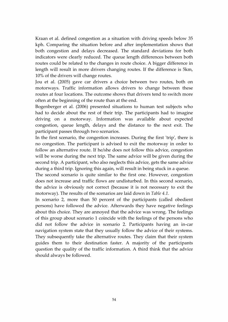
54
Kraan et al. defined congestion as a situation with driving speeds below 35
kph. Comparing the situation before and after implementation shows that
both congestion and delays decreased. The standard deviations for both
indicators were clearly reduced. The queue length differences between both
routes could be related to the changes in route choice. A bigger difference in
length will result in more drivers changing routes. If the difference is 5km,
10% of the drivers will change routes.
Jou et al. (2005) gave car drivers a choice between two routes, both on
motorways. Traffic information allows drivers to change between these
routes at four locations. The outcome shows that drivers tend to switch more
often at the beginning of the route than at the end.
Bogenberger et al. (2006) presented situations to human test subjects who
had to decide about the rest of their trip. The participants had to imagine
driving on a motorway. Information was available about expected
congestion, queue length, delays and the distance to the next exit. The
participant passes through two scenarios.
In the first scenario, the congestion increases. During the first ʹtripʹ, there is
no congestion. The participant is advised to exit the motorway in order to
follow an alternative route. If he/she does not follow this advice, congestion
will be worse during the next trip. The same advice will be given during the
second trip. A participant, who also neglects this advice, gets the same advice
during a third trip. Ignoring this again, will result in being stuck in a queue.
The second scenario is quite similar to the first one. However, congestion
does not increase and traffic flows are undisturbed. In this second scenario,
the advice is obviously not correct (because it is not necessary to exit the
motorway). The results of the scenarios are laid down in Table 4.1.
In scenario 2, more than 50 percent of the participants (called obedient
persons) have followed the advice. Afterwards they have negative feelings
about this choice. They are annoyed that the advice was wrong. The feelings
of this group about scenario 1 coincide with the feelings of the persons who
did not follow the advice in scenario 2. Participants having an in‐car
navigation system state that they usually follow the advice of their systems.
They subsequently take the alternative routes. They claim that their system
guides them to their destination faster. A majority of the participants
question the quality of the traffic information. A third think that the advice
should always be followed.
55
Scenario 2
Exits the motor‐way during the
first trip
During the second
trip
During the third
trip
Does not exit the motorway
(critical person)
TOTAL
Exits the motor‐way during the first trip
97(obedient persons)
4 0 3 104
During the second trip
2 4 5 23 34
During the third trip
0 2 0 15 17
Does not exit the motorway (critical person)
1 1 2 5 9
Scenario 1
TOTAL 100 11 7 46 164
Table 4.1. Decision to exit the motorway according to scenarios and to trips (in numbers of
human test subjects)
Conclusions
A series of variable messages signs on an urban ring road showed some
effect on route choice. The queue length differences between both routes
could be related to the changes in route choice. A larger difference in length
will result in more drivers changing routes
At the beginning of a route, more route changes are made than at the end.
In an experimental design, 50 percent of the participants follow the advice to
exit the motorway, even if the advice is obviously not correct. Almost a third
does not follow this advice, even in conditions confirming the correctness of
the advice.
4.3. Navigation systems
DVS (2008) reports about a questionnaire survey amongst 202 car drivers
using a navigation system. Most of the drivers (60%) in this survey drive at
least 20,000 kilometres a year in their own car or in a company car. For
commuting, almost 70 percent never uses the navigation system. The system
is used for business trips and recreational trips in particular.
Vonk et al. (2007) investigate data about 1,144 car drivers. Within this group,
28 percent have a navigation system. According to Vonk et al., this
percentage is higher than that in other studies (average 20%). Around 35
percent of car drivers having a navigation system use their system in 20
percent of their trips. Around 15 percent use the system in 80 percent of their
56
trips. The system is mostly used for unknown destinations. Car drivers
having a navigation system drive more kilometres a year than drivers
without a system do. Sixty percent of the system owners drive more than
20,000 km a year; only forty percent of the non‐owners drive that distance.
According to DVS (2008), 86 percent of the car drivers having a navigation
system use the setting ʹfastest routeʹ. Only a few drivers use ʹshortest routeʹ.
The main reasons for using a navigation system are: arriving at the
destination as fast as possible and a prevention of making detours (each
reason was mentioned by 40 percent).
A navigation system informing about the current traffic situation can draw
the attention of the driver in time to be prepared for coming events. A driver
could change routes because of this advice. One fifth of the respondents in
the DVS survey use the option to change routes, given the information about
congestion. What would happen if a greater number of drivers would change
routes? This effect is still unknown. Over a third of the respondents choose a
route without using the (potentially available) information about current or
frequent queues.
The road classification used in the navigation system will largely determine
the advised route choice. That is because a road class has a characteristic
speed limit; this limit is used for calculating travel times, thus determining
the fastest route. However, what would road classification look like from a
safety point of view? Map producers use more and other road types than
Sustainable safety does (VIA, 2007). The road user is led to ʹhigherʹ road
types as soon as possible. This corresponds with the requirements regarding
functionality in Sustainable Safety. Navigation system users claim to drive on
motorways (32%) and rural main roads (28%) more often than they would
without such a system (DVS, 2008). They also drive on access roads (16% in
rural areas, 15% in urban areas) more often; according to the drivers, these
roads were advised by the system. The respondents (users of navigations
systems) to the survey of Vonk et al. (2007) reported they drove more on
highways (18%), secondary roads (17%), and urban roads (6%). Of the road
types in these answers, the motorway has the lowest crash risk. For road
safety reasons, it is desirable that a greater part of trip lengths is covered by
motorways. Vonk et al. also investigated the mental stress of drivers by using
system‐equipped vehicles in a small‐scale experiment (36 drivers). Drivers
using a navigation system experienced less stress and mental effort than
drivers without a system did. This result was based on both the driversʹ
opinion and on measurements. The drivers followed routes in an area
unknown to them. The system users drove shorter distances (‐16%), and
spent less travel time (‐18%). This result was reached by fewer stops (in time)
57
and by using more route length on motorways. Given less exposition (time
and distance), the crash frequency would be lower.
4.4. Conclusions
Conclusions regarding route choice
A significant number of drivers makes a well‐founded decision when
choosing an alternative route on account of a changer in circumstances. This
decision is a weighting of risk (of not adapting) and advantages (of
adapting). Personal preferences are less important than was assumed. The
context of the trip and the nature of the changing circumstances
(disturbance) are also relevant. Drivers have a strong need for up‐to‐date
information. Some drivers deliberately opt for the motorway because
information will more often be available on that road type.
Travel time and trip length are without a doubt the most important factors in
route choice. For business trips and commuting, these factors are often
mentioned. However, travel time and trip length sometimes appear
subjective rather than objective values. The number of stops and traffic
volumes are related factors for route choice. The road environment (urban
planning aesthetics, scenery) will also influence route choice. Prior knowledge
about a route is of more importance for route choice than perceived route
characteristics, which are in their turn, more important than objective
characteristics.
Drivers prefer a less congested route as well as (parts of) routes on
motorways; they also prefer good road and weather conditions, less stress,
and fewer idle stops. Motorways are very much preferred; they are
associated with a low stress level.
A driver who frequently travels to the same destination, changes routes most
often. They prefer routes with less access, particularly motorways. Road
safety is not an issue in route choice matters. The number of selected routes
depends on the type of area (rural or urban) as well as on the volumes on the
main road network. Most drivers use two or three routes.
Conclusions regarding the steering or influencing of route choice
Prior to a trip, a significant number of drivers take note of traffic information,
mostly by radio, television or the Internet. This information will largely
determine route choice or departure time. The traffic information en route is
obtained by way of radio, personal observation, variable message systems,
and for some drivers, a navigation system. A substantial number of drivers
change routes because of this information. Commuters can be divided into
58
groups differing in flexibility regarding departure time, the likelihood of
changing routes on account of prior information, or searches for prior
information, and stress on the preferred route.
A series of variable messages signs on an urban ring road showed some
effect on route choice. The queue length differences between both routes
could be related to the changes in route choice. A bigger difference in length
will result in more drivers changing routes
At the beginning of a route, more route changes are made than at the end.
In an experimental design, more than 50 percent of the participants follow
the advice to exit the motorway, even if the advice is obviously not correct.
Almost a third does not follow this advice, even in conditions confirming the
correctness of the advice.
A fifth to a quarter of car drivers in the Netherlands own a navigation
system. They drive more than average distances a year; they use their
navigation systems for unknown destinations.
The expected total effect of navigation systems is: less exposition and less
stress for the driver. It is yet unknown what would happen if a greater
number of drivers changed their routes. This would certainly affect the traffic
circulation in the road network and is a matter deserving further study.
59
5. Road safety aspects of road network structure
and road classification
Road classification, geometrics, legislative rules, and traffic circulation are
interrelated. Changes in one of these four factors will affect the other three.
For instance, a measure in one street (one‐way traffic) may result in a change
in traffic circulation in the surrounding area. Sometimes this will cause a
difference between the intended function (according to the classification) and
the actual function. Another outcome may be a discrepancy between the road
design (e.g. a narrow lane) and the actual traffic situation (e.g. a great deal of
traffic in both directions).
This interaction needs to be understood to find out why problems arise. This
understanding will facilitate more appropriate traffic measures which will
affect the interaction most effectively. The present study aims to identify
traffic measures that, first and foremost, have positive road safety effects.
In order to find out the consequences of changes in the four areas described
above, knowledge is needed about road safety aspects of both road
classification and all other kinds of traffic provisions. Road safety aspects are
usually expressed in terms of numbers of crashes or numbers of casualties
per annum. Subsequently, the absolute numbers have to be related to the
exposure to risk, mostly expressed by the number of motor vehicles or the
number of motor vehicle kilometres. In many cases, these kinds of data are
unknown, either on account of lacking evaluations or because of
methodological problems. For instance, from a methodological point of view
it is impossible to show an effect of one traffic hump on the number of
crashes. Intermediate indicators are available to show an effect after all, in
this case driving speeds near the hump. In general, to gain a good insight
into road safety more indicators have to be used than the number of crashes
only.
Crash analysis has become less important with the introduction of the
Sustainable Safety approach. That is because this approach uses general
safety knowledge for setting requirements and specifying rules for road
classification and road design. The knowledge translated into these
requirements and rules is meant to prevent crashes or, if a crash is inevitable,
reduce the severity of the crash. In order to achieve these aims large
differences in speeds (zone 30), in driving directions (barrier) and in masses
60
(bicycle path) should be avoided. A systematic check of the existing or
planned (parts of the) road network will make clear whether the
requirements have been met.
On the level of road networks, a change in structure and/or in road
classification will mostly affect traffic circulation, departure times and modal
choice. The changes may be of a complex nature. That is why traffic
modelling is used to find possible effects.
This Chapter 5 gives an overview of three types of studies:
1. Studies using a large number of variables in order to describe road
structure and travel behaviour. Accordingly, these variables are related
to crash figures resulting in statistical models. Such models show the
quantitative relationships between the variables and the crash numbers.
2. Studies demonstrating the relationships between, on the one hand,
characteristics regarding network structure, accessibility, road
classification, and road design and, on the other hand, traffic volumes.
Changes in traffic volumes are used as an indicator for the impact on
traffic nuisance and unsafety.
3. Studies regarding the direct relationships between the characteristics
mentioned at 2., and crash figures.
Studies of the second and third type can be modelling studies and
before/after studies. Mostly, the characteristics are changed on the input side
(in the model or in reality), while the effects on traffic volumes and on crash
numbers (the output) are to be evaluated.
5.1. Network structure and travel behaviour related to crash
numbers
This section deals with studies estimating statistical models regarding
relationships between various variables and crash numbers. This section
seeks to answer the question whether objective characteristics concerning
urban areas, road infrastructure, traffic and transport are statistically related
to crash frequency. This (statistical) approach usually shows significant and
non‐significant relationships. It cannot always be understood why the one
relationship is significant and the other one is not. In some cases, it has to do
with the number of observations, in other cases with the lack of variance
within a variable. Sometimes, relationships are hidden because important
variables are missing in the model.
Hadayeghi et al. (2003) gathered data from 463 traffic zones in Toronto
(Ontario, Canada) regarding socio‐economics, traffic, population, and
61
crashes. The traffic data consisted of the number of intersections, intersection
density, length of main roads, length of other roads, speed limits (posted
speed), volume to capacity ratio (V/C), inbound and outbound traffic, and
the number of motor vehicle kilometres. The authors use models having a
negative binomial distribution (of the parameter for ʹoverdispersionʹ, i.e.
extra variation). According to Miaou (1994), this distribution is better than
the Poisson distribution (that was used by many other authors). Hadayeghi
et al. (2003) built models for the total number of crashes, serious crashes, and
crashes during the morning rush hour (total and serious). The models for the
rush hour prove to be better than those for the entire day, probably because
the traffic data refer to the rush hour only. The best model (total number of
crashes during rush hour) comprises the following significant variables: road
length, number of employed, volume to capacity ratio, and speed limits.
Another type of model was also applied: the geographically weighted
regression model. This type of model allows for a spatial distribution of the
variables. It comprises the following significant variables: speed limits,
volume to capacity ratio, number of households, intersection density, and
road length. This model produces a better result than the binomial models.
Hadayeghi et al. (2007) continued the work described above. A follow‐up
study was set up to estimate a risk model. This was done by using
generalized linear modelling, assuming a negative binomial distribution. In
total, 23 models were analyzed: twelve for all crashes, eleven for serious
crashes. Some models contain variables describing traffic and network
structure. Other models (called comprehensive models) comprise a few of the
preceding variables as well as socio‐economical and demographic variables.
The comprehensive models have the better statistical results. The best model
predicts the number of (serious) crashes by using the following variables:
number of motor vehicle kilometres, road length, number of signalized
intersections, size of commercial and industrial area, and number of
inhabitants.
Ladrón de Guevara et al. (2004) used data from 859 traffic zones in the urban
area of Tucson (Arizona, U.S.A.). These data regard socio‐economical and
demographic variables as well as traffic and crash variables. All models have
a negative binomial distribution. Models were estimated for fatal crashes,
injury crashes, the sum of these two types of crashes, and crashes with
damage only. The model for the sum of fatal and injury crashes produced the
best results. In this model, intersection density and road length are
significant variables. The additional significant variables are population
density and number of employees. The authors do not allow for spatial
distribution of the variables, as Hadayeghi et al. (2003) did.
62
Quddes (2008) set up several models for explaining the number of casualties
in 633 London wards (= city districts). His models contain variables
regarding traffic, road and socio‐demographic characteristics. The traffic
variables are volumes and average driving speed; the road variables are
number of intersections (and roundabouts), road length per road type,
curvature, and number of bus stops. The socio‐demographic variables are
resident population younger and older than 60 years, number of employees,
number of households without a car. The number of motor vehicle
kilometres was unknown. Therefore, an estimation of the average number of
motor vehicles in a ward was used as an indicator for exposure. The
statistical models used can be split up into two groups: non‐spatial and
spatial models. The non‐spatial models having a negative binomial
distribution do not allow for spatial dependency of the wards, the spatial
models do. The non‐spatial models appear to have the following significant
variables: resident population older than 60 years, length of main roads and
residential streets, and average driving speeds. The number of intersections
was not significant, neither was the number of bus stops. The spatial models
have about the same results. However, the average driving speed is not
significant in the spatial models. In the non‐spatial models, driving speed
was negatively correlated with the number of casualties meaning that a
higher speed would result in fewer crashes. This result (only to be expected
on motorways) is absent in the spatial models. For road structure and
classification, Quddesʹ concludes that curvature is not significant, while
traffic volumes and length of main roads and residential streets are positively
correlated with the number of casualties. The number of intersections and
the number of bus stops did not appear to be significant.
5.2. Relating characteristics of network structure, degree of
access, road classification and road design to
traffic volumes
Quantitative relationships between various characteristics regarding network
structure and traffic on the one hand and traffic volumes on the other hand
are the subject of this section. Traffic volumes are regarded to be an
important intermediate variable regarding road safety. The assumption is
that lowering of traffic volumes will improve road safety and traffic
nuisance.
63
The studies discussed below were conducted by using traffic modelling.
Section 5.3 is meant to check whether the results in this section are supported
by empirical evidence.
Van Minnen (1999) studied the effects of the number of accesses to a
residential area on the traffic volumes in the residential streets of that area.
For this purpose, he used a simulation model. The inputs of the model were
size of the areas, dwelling density and number of accesses; the output
comprised the volumes in the streets accessing the area, and the length of the
trips entering the area (including the part of the trip using the roads
surrounding the area). In all cases, he used a grid network structure, in a
square type of area. Van Minnen assumed five car trips a day to and from
each dwelling unit. This value originated from Walraad & Poppe (1998).
Table 5.1 shows the simulation results. According to CROW (2004) the
maximum acceptable volume in residential streets is 3,000 to 5,000 motor
vehicles a day, depending on the spatial position of the area (highly
urbanized or hardly urbanized). These values are only based on a few
observations, and not based on systematic empirical research. In Table 5.1,
these acceptable daily volumes (between 3,001 and 5,000 vehicles) have been
highlighted (bold boxes).
The results are that the size of the area has no detrimental effects on the total
number of motor vehicle kilometres (roads inside and outside the area)
provided that (Van Minnen, 1999; p. 18):
there are accesses to the area on all (four) sides,
the number of accesses per unit length is sufficient (i.e. resulting in
acceptable volumes of motor vehicles in residential streets).
A wider area will result in higher volumes on some streets in the area. Van
Minnen concluded that a singular (public) access is only acceptable for areas
smaller than 30 ha. The number of accesses increases substantially when the
size is between a 100 and 200 ha. Van Minnen only used a model for an
ʹisolated areaʹ with surrounding roads which are not connected to the rest of
the network. The connections between the area and the surrounding roads
may vary in number and position. Krabbenbos et al. (2002) focused on this
topic, using a micro‐simulation model (AIMSUN). They modelled a square
area (640 x 640 m2). The surrounding roads are connected to the rest of the
network either at the angular points or in the middle of each side of the
square. The area has a grid network structure with three streets in each
direction. The speed limit on the surrounding roads is 50 km/h, and on the
residential streets 30 km/h. The connections to the rest of the network were
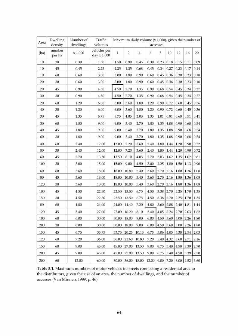
64
Area Dwelling
density
Number of
dwellings
Traffic
volumes
Maximum daily volume (x 1,000), given the number of
accesses
(ha) number
per ha x 1,000
vehicles per
day x 1,000 1 2 4 6 8 10 12 16 20
10 30 0.30 1.50 1.50 0.90 0.45 0.30 0.23 0.18 0.15 0.11 0.09
10 45 0.45 2.25 2.25 1.35 0.68 0.45 0.34 0.27 0.23 0.17 0.14
10 60 0.60 3.00 3.00 1.80 0.90 0.60 0.45 0.36 0.30 0.23 0.18
20 30 0.60 3.00 3.00 1.80 0.90 0.60 0.45 0.36 0.30 0.23 0.18
20 45 0.90 4.50 4.50 2.70 1.35 0.90 0.68 0.54 0.45 0.34 0.27
30 30 0.90 4.50 4.50 2.70 1.35 0.90 0.68 0.54 0.45 0.34 0.27
20 60 1.20 6.00 6.00 3.60 1.80 1.20 0.90 0.72 0.60 0.45 0.36
40 30 1.20 6.00 6.00 3.60 1.80 1.20 0.90 0.72 0.60 0.45 0.36
30 45 1.35 6.75 6.75 4.05 2.03 1.35 1.01 0.81 0.68 0.51 0.41
30 60 1.80 9.00 9.00 5.40 2.70 1.80 1.35 1.08 0.90 0.68 0.54
40 45 1.80 9.00 9.00 5.40 2.70 1.80 1.35 1.08 0.90 0.68 0.54
60 30 1.80 9.00 9.00 5.40 2.70 1.80 1.35 1.08 0.90 0.68 0.54
40 60 2.40 12.00 12.00 7.20 3.60 2.40 1.80 1.44 1.20 0.90 0.72
80 30 2.40 12.00 12.00 7.20 3.60 2.40 1.80 1.44 1.20 0.90 0.72
60 45 2.70 13.50 13.50 8.10 4.05 2.70 2.03 1.62 1.35 1.02 0.81
100 30 3.00 15.00 15.00 9.00 4.50 3.00 2.25 1.80 1.50 1.13 0.90
60 60 3.60 18.00 18.00 10.80 5.40 3.60 2.70 2.16 1.80 1.36 1.08
80 45 3.60 18.00 18.00 10.80 5.40 3.60 2.70 2.16 1.80 1.36 1.08
120 30 3.60 18.00 18.00 10.80 5.40 3.60 2.70 2.16 1.80 1.36 1.08
100 45 4.50 22.50 22.50 13.50 6.75 4.50 3.38 2.70 2.25 1.70 1.35
150 30 4.50 22.50 22.50 13.50 6.75 4.50 3.38 2.70 2.25 1.70 1.35
80 60 4.80 24.00 24.00 14.40 7.20 4.80 3.60 2.88 2.40 1.81 1.44
120 45 5.40 27.00 27.00 16.20 8.10 5.40 4.05 3.24 2.70 2.03 1.62
100 60 6.00 30.00 30.00 18.00 9.00 6.00 4.50 3.60 3.00 2.26 1.80
200 30 6.00 30.00 30.00 18.00 9.00 6.00 4.50 3.60 3.00 2.26 1.80
150 45 6.75 33.75 33.75 20.25 10.13 6.75 5.06 4.05 3.38 2.54 2.03
120 60 7.20 36.00 36.00 21.60 10.80 7.20 5.40 4.32 3.60 2.71 2.16
150 60 9.00 45.00 45.00 27.00 13.50 9.00 6.75 5.40 4.50 3.39 2.70
200 45 9.00 45.00 45.00 27.00 13.50 9.00 6.75 5.40 4.50 3.39 2.70
200 60 12.00 60.00 60.00 36.00 18.00 12.00 9.00 7.20 6.00 4.52 3.60
Table 5.1. Maximum numbers of motor vehicles in streets connecting a residential area to
the distributors, given the size of an area, the number of dwellings, and the number of
accesses (Van Minnen, 1999; p. 46)
65
varied according to the number of sides having a connection and to the
number of connections at each side, resulting in 16 variants. The dwelling
density of the area amounts to 40 dwellings per ha. The assumption for the
number of trips per dwelling unit during rush hour is 0.46 trips. This value
looks quite different from that which Van Minnen used (five trips a day).
However, Krabbenbos et al. take 10 percent of the daily trips as the rush hour
volume. Ten percent out of five trips (= 0.5) is close to the value of 0.46.
The next variable in Krabbenbosʹ study is the degree of through traffic (traffic
not having an origin and destination within the area). The degree of this type
of traffic was assumed to be either high or low. The amount of local traffic
(with origin or destination within the area) amounted to 760 vehicles, the low
through traffic value was 534 vehicles, and the high value was 3,740 vehicles.
The simulations did not show a specific rule regarding neither the optimal
number of connections nor the position of the connections. This appears to
depend on the connection of the rest of the network to the area (at the
angular points or in the middle of each side), and on the amount of through
traffic. The access of the area to the surrounding roads will determine the
amount of through traffic; the connections in the middle of each side offer
the ʹbestʹ short cuts, because through traffic can pass the area without any
detour (compared to the route surrounding the area). The connections at the
angular points will offer a route which is just as long as the route following
surrounding roads. The route surrounding the area will be more attractive
because of the higher speed limits. Krabbenbos et al. (2002) gathered
empirical data from four residential areas. These areas differed regarding the
number of connections and the position of these connections. The degree of
through traffic and the amount of local traffic was estimated. However, the
number of observations was small and a reference (or control) area was
lacking. That is why only a conclusion regarding the local traffic could be
drawn. The more sides (of the square) are connected to the surrounding
roads, the lower the number of vehicle kilometres of local traffic.
Gadd (1997) analyzed how goals regarding capacity, road safety and
environment can be attained simultaneously. For his evaluation, Gadd built a
simulation model of a simple (synthetic) network consisting of a main road
surrounding a square area. Within the area, two distributors cross each other
diagonally. The main road is connected to the rest of the network at the
angular points. In a first simulation, all roads belong to the same class; the
intersections are non‐signalized. The simulation shows a great deal of traffic
on the distributors (to a maximum of half the amount on the main road). The
main road is upgraded in the next simulation; the intersections at the angular
66
points have signalization. The intersections within the area have regular
priority rules. The results of simulating this new situation are: the volumes
on the distributors are not more than a quarter of the volumes on the main
road, and the number of motor vehicle kilometres (on both road types)
increases by 3 percent. A third simulation keeps the classification as well as
the signalization as they were (in the second simulation). However, the
intersections within the areas are now stop sign controlled. Now the
remaining volumes on the distributors are only 21 percent at the most related
to the main road volumes; the motor vehicle kilometres did not change
anymore. The final, fourth, simulation concerns a change of the intersections
within the area; an additional delay was introduced. Now, the distributors
carry only 9 percent of the amount of traffic on the main roads; again, the
number of motor vehicle kilometres has not changed. Obviously, the
resistance for through traffic was raised to such an extent that only a fraction
was left. Road safety and the road environment within the area have
improved by these measures. The volumes on the main road have increased
by 20 percent. Specific measures are needed to balance the favourable effects
within the area against the deteriorating effects (by the increasing number of
motor vehicles) on the main road.
Skoupil et al. (1983) evaluated the effects of changing traffic circulation. The
street network of five residential areas was modelled in order to find the
effect of closing some streets for motorized traffic. The models were
calibrated for the existing situation including through traffic. The street
closures were only modelled; not applied in practice. The modelled street
networks comprise distributor roads (within the residential areas),
surrounding main roads, and some connecting external roads. These roads
fall into a larger area containing almost all origins and destinations of trips to
and from the (five) residential areas; this was found in a street survey. The
changes in circulation of traffic were studied for each area. The number of
motor vehicle kilometres was calculated for each street type. Traffic
circulation changed largely because of the street closures. In four of the five
areas, two systems of closures were applied:
Vehicles could still pass through the entire area; some streets received a
new design; on some intersections drivers were not allowed to turn into
each direction; some streets changed into a cul‐de‐sac.
The area was divided into zones; vehicles could only travel within a
zone, and not pass through the entire area anymore.
Both systems reduce the amount of through traffic substantially. The second
system (zones) shows the largest reduction in three out of four cases. The
67
fifth and final area was adapted by mainly using one‐way streets, which also
reduced through traffic successfully. Skoupil et al. (1983) specifically
investigated the effects on local traffic (having origins or destinations within
one of the areas). All circulation systems raise the number of motor vehicle
kilometres for local traffic. The zone system shows the lowest number of
vehicle kilometres on streets within the area compared to both the before
situation and to the other closure system. However, the zone system resulted
in more kilometres on the surrounding roads and on the other connecting
roads than the other system did.
5.3. Relating characteristics of network structure, degree of
access, road classification and road design to
crash figures
This section deals with the direct effects of network structure and road
features on crash frequency or risk. Contrary to Section 5.1, differences
between situations were studied; particularly comparing existing situations
(comparative empirical studies), comparing several future situations
(modelling studies), or comparing before and after situations (before‐/after
studies).
Marks (1957) reports on an accident study carried out in Los Angeles. Two
traffic structures were examined: a grid system and a system with limited
access. The grid system showed almost eight times as many accidents as the
limited access system. At four‐arm junctions, the number of accidents per
year per junction was three times higher than in the limited access system.
According to Marks (1957), a safe design is characterised by:
a limited access system, preferably with access roads approximately 350
metres apart (a distance that was also mentioned by Le Corbusier in
1924)
no streets linking two main roads
(local) distributor roads to be included only if they do not cross
through‐streets and only when they join arterial roads on one side only
junctions with four arms are to be avoided wherever possible in favour
of simple T‐junctions
These recommendations were rediscovered years later and formed part of
the major Dutch ʹDemonstratieproject herindeling en herinrichting van
stedelijke gebiedenʹ (Demonstration project in the reclassification and
redesign of urban areas) (Janssen & Kraay, 1984). Two large residential areas
68
and the surrounding main roads (situated in the cities of Eindhoven and
Rijswijk) were changed radically. The project aimed at reducing through
traffic in residential areas, improving traffic flow on the main roads, and
reducing driving speeds in residential streets. The measures taken appeared
to be very effective; in particular because most of the through traffic
disappeared. The measures taken can be divided into three types, called
options:
1. Introducing mainly one‐way traffic
2. Building speed‐reducing provisions, partly combined with one‐way
traffic
3. Introducing the ʹwoonerfʹ (home zone) street design type
At the start of the project, the assumption was that these three options would
have different effects. This appeared not to be true. Hardly any differences
showed up. Differences between areas regarding reductions in through
traffic could not be related to the options. Differences between areas
concerning road design or traffic circulation could not explain the level of
through traffic. In general, through traffic can be reduced by making an area
physically unattractive for rat running, and by improving (traffic flow on)
the surrounding roads.
Janssen (1991c) evaluated the effects of these three options on both the
number of crashes and on crash risk. The crash evaluation is subjected to a
before period from 1972 to 1977, and an after period from 1982 to 1986. The
years in between are not used for the evaluation because at that time the
redesigning was implemented. In the residential areas the number of injury
crashes decreased by 80 percent; this decrease was adjusted for the general
trend. The injury crash risk was reduced by 75 percent in the residential
areas, and by 16 percent on the surrounding main roads. The number of
motor vehicle kilometres dropped by 30% in the residential areas, and
increased by a few percentages on the main roads. The measures appeared to
be successful, not only for reducing through traffic, but also for improving
road safety. The small differences between the options were considered an
unexpected result. The provisions applied in the experimental residential
areas fit into the design practices of the eighties applying all features of area‐
wide traffic calming schemes (VenW, 1984). In the late nineties, the Start‐up
Programme of Sustainable Safety (VNG, IPO, VenW & UvW, 1998) was the
beginning of a trend towards a more low‐cost design of residential areas. The
effects of this trend tend to be less beneficial for road safety (Berends &
Stipdonk, 2009).
Parallel to the demonstration project, some other European countries did
similar large‐scale projects and evaluations. In (West) Germany, Pfundt et al.

69
(1979) showed that in residential areas the number of injury crashes dropped
by more than 40 percent. On the surrounding roads of these areas, the
numbers of injury crashes decreased too, although to a lower extend. The
effects found in the German projects are substantial, although smaller than in
Eindhoven‐Rijswijk.
Engel & Thomsen (1983) reported about the effects of reclassification and
redesigning in the district Østerbro of Copenhagen, the Danish capital. In
this district, the number of casualties dropped by 40 percent (adjusted for the
general trend). This project shows large effects too.
Obviously, substantial effects can be attained if reclassification and
redesigning are applied on a district level.
Dijkstra & Van de Pol (1991) estimated the effect on road safety of the new
Amsterdam ring road (motorway A10) in 1989‐1990. The authors used
general safety indicators for estimating the expected changes. The approach
in this type of study is to classify roads according to a system used by
Janssen (1988) and Dijkstra (1990). The safety level of the existing situation is
checked by retrieving the crash history (three years) of each road class.
Subsequently the length and average daily traffic volume of each road class
is used in order to find the number of motor vehicle kilometres. Combining
these figures with the crash numbers will result in the crash risks for each
road class. In these kinds of estimations the assumption usually is that the
risk (per road class) will not change in the after period. Adding a new
motorway was not the only change; some urban roads were reclassified, a
few connections were added, and some roads were upgraded (mainly by
adding lanes). The new network was modelled by means of a transport
model. The results from the model show a changed traffic circulation,
resulting in other volumes for nearly each road class. The figures for the
motor vehicle kilometres had to be adapted accordingly to these new
volumes. Finally, the numbers of crashes were estimated for each road class.
The expected number of crashes would drop by 3.5 percent (minus 64
crashes on a total number of 1,762). The decrease on some urban main roads
(‐145) would partially be ʹcompensatedʹ by an increase (+80) on the
motorways and some rural main roads. The conclusion is that adding a new
motorway does not ʹautomaticallyʹ benefit road safety enormously, since
traffic circulation is thoroughly affected which may result in negative effects
on some roads.
Poppe (1997) estimated the effects of applying the Sustainable Safety road
classification to the road network in the central part of the Netherlands
(province of Utrecht supplemented by a few relevant areas). The road
70
classification in the existing macro model had to be adapted according to the
principles of Van Minnen & Slop (1994). One of these principles is the so‐
called ʹtrip duration criterionʹ, meaning that that part of a trip which is
travelled on access roads (speed limit of 30 km/h in urban areas and 60 km/h
in rural areas) should not last longer than 3 minutes. The residential areas,
rural and urban, should be kept free from through traffic. The roundabout, a
new phenomenon on distributor roads, was applied to a large extent. The
network structure did not change very much. The accessibility of residential
areas was somewhat limited; hierarchical (tree) structures were avoided as
much as possible to prevent detours. Poppe compared the effects of two
network structures: the structure proposed by the regional authority for the
year 2010 (the so‐called MIT option), and the Sustainable Safety structure.
The key safety indicators (risks per road class) were taken from SWOV
(1997). The results show differences in traffic circulation because of the
differences in road classification and speed limits. The number of casualties
in the Sustainable Safety option is about 6 percent lower than in the MIT
option. The number of motor vehicle kilometres in the Sustainable Safety
option and the number of ʹmoving vehicle hoursʹ (vehicles actually driving)
nearly equals the MIT option. The number of lost hours (vehicles waiting at
intersections) is considerably lower (15 percent) in the Sustainable Safety
option than in the MIT option. This can be explained by the shorter waiting
times at roundabouts compared to the waiting times at signalized
intersections. The conclusion is that, despite of the lower speed limits, the
Sustainable Safety network functions quite well.
Lovegrove & Sayed (2006, 2007) take the approach of Hadayeghi et al. (2003)
and Ladrón de Guevara et al. (2004) as a starting point. They derived 47
crash prediction models (CPMs) from 22 variables. They put these models
into 16 groups; see Table 5.2.
Some of the variables were quantified by way of a traffic model. Lovegrove
& Sayed (2006) applied their prediction models to three districts having a
specific network structure for traffic calming (reducing through traffic). The
results of their models for the three districts together conform quite well to
the observed crash reductions. The results for each of the districts separately
show larger differences between modelled and observed crash reductions.
The authors investigated network structures proposed by Dijkstra (1996).
These network structures can also be found in the guidelines for Sustainably
Safe urban roads (Infopunt DV, 2000). The network structures are limited
access, grid and tree; see Figure 5.1, structures a, b and c. The authors added
an additional structure containing three‐way intersections only; this structure
allows for through routes (see Figure 5.1, structure d).
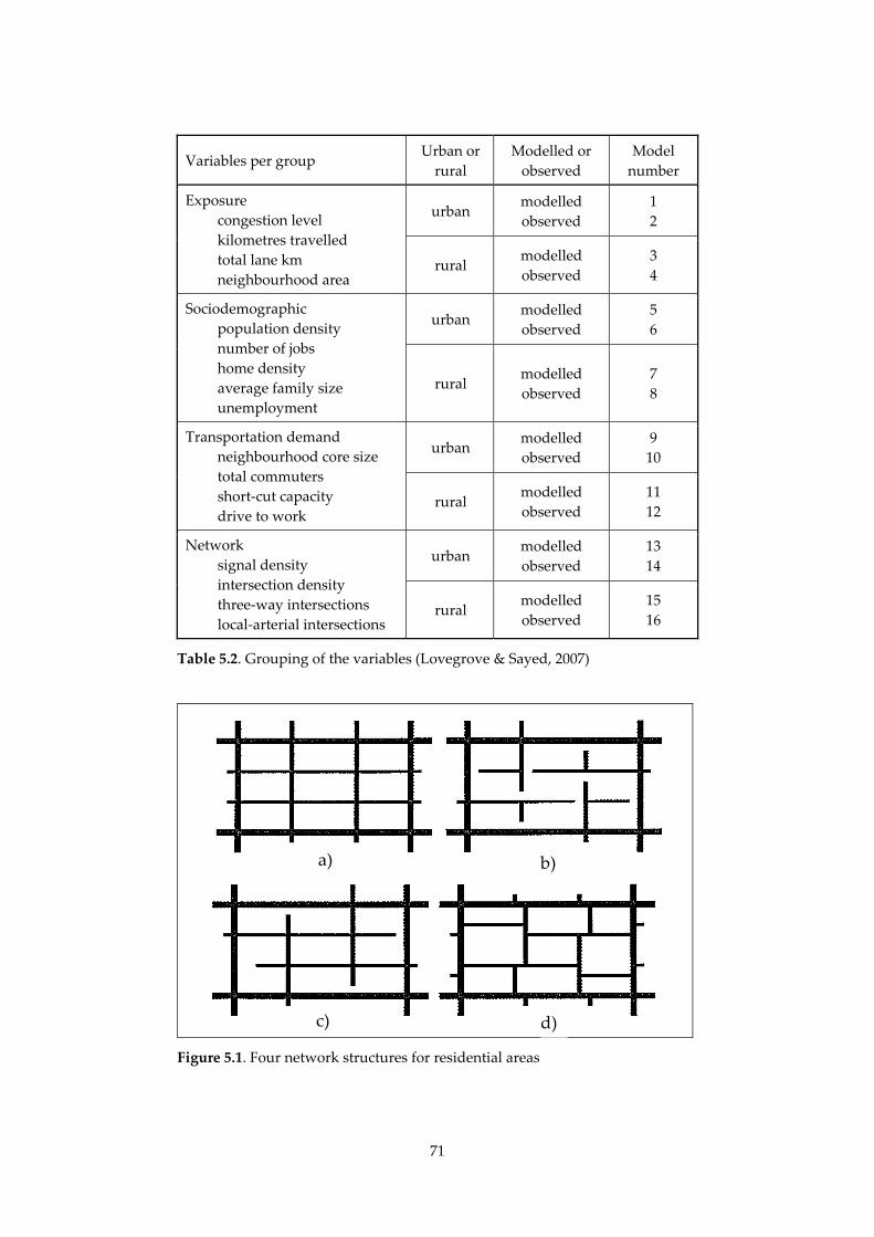
71
Variables per group Urban or
rural
Modelled or
observed
Model
number
urban modelled
observed
1
2
Exposure
congestion level
kilometres travelled
total lane km
neighbourhood area rural
modelled
observed
3
4
urban modelled
observed
5
6
Sociodemographic
population density
number of jobs
home density
average family size
unemployment
rural modelled
observed
7
8
urban modelled
observed
9
10
Transportation demand
neighbourhood core size
total commuters
short‐cut capacity
drive to work rural
modelled
observed
11
12
urban modelled
observed
13
14
Network
signal density
intersection density
three‐way intersections
local‐arterial intersections rural
modelled
observed
15
16
Table 5.2. Grouping of the variables (Lovegrove & Sayed, 2007)
Figure 5.1. Four network structures for residential areas
d)c)
a) b)
72
The variables in the crash prediction model for this case were estimated by
observations in areas resembling those with the structures shown in
Figure 5.1. The crash density of structure type ʹdʹ (Figure 5.1) appears to be
the lowest, followed directly by limited access (structure type ʹcʹ). The limited
access structure was somewhat adapted by the authors using three‐way
intersections instead of four‐way intersections. The differences between the
calculated crash densities and the average densities of existing residential
areas appear to be small. The highest crash densities are found for the grid
structure, both higher compared to the calculated values for the other
structures and to the empirical average value of all structures. Rifaat & Tay
(2009) came to similar conclusions using data from residential areas in
Calgary.
5.4. Conclusions
Several statistical models were developed relating variables regarding socio‐
economical, demographic, traffic, and network structure factors on the one
hand to numbers of crashes or casualties on the other hand. Variables
showing a strong relationship with road safety are:
Speed limit, volume to capacity ratio, number of households,
intersection density, and road length (Hadayeghi et al., 2003)
Number of kilometres travelled, road length, number of signalized
intersections, size of commercial and industrial area, and number of
inhabitants (Hadayeghi, 2007)
Intersection density and road length per road class, population density,
and number of employees (Ladrón de Guevara et al., 2004)
Resident population older than 60, traffic volume, length of main roads
and residential streets (Quddes, 2008); according to this author, the
following variables on the level of city districts are not related to road
safety: average driving speed, number of intersections and
roundabouts, and number of bus stops
Results for studies relating characteristics of network structure, degree of
access, road classification and road design to traffic volumes or crash
figures
The lowest crash density can be found in a network structure only
having three‐way intersections, although allowing for through routes.
The limited access structure shows a somewhat higher crash density.
The highest crash density belongs to the grid structure.
73
The level of through traffic in a square sized residential area (grid
network) is determined by the number and the position of the
connections of the local network to the external network. Connections
in the middle of the sides offer the fastest through routes (no detours).
Connections at the angular points will result in through routes which
are just as long as routes along the surrounding roads. The latter route
will be more attractive because of the higher speed limits on these
roads. The more sides of an area are connected, the shorter trip length
for local traffic is (origin or destination within the area).
Several traffic measures in a residential area (one‐way traffic, street
closures, barring some turning directions on intersections, internal
zoning, and speed reducing provisions) will mostly diminish through
traffic because of the higher resistance of the through routes. Both the
local environment and road safety will benefit from these measures.
Traffic volumes on the surrounding road will mostly increase. The
worsening conditions on the surrounding mains roads should be
outweighed by improvements in the areas.
A regional network classified according to Sustainable Safety will most
probably result in a lower number of casualties than a traditional
network. The large numbers of roundabouts in the Sustainable Safety
network will decrease the amount of vehicle hours spent on waiting at
signals.
Before‐ and after‐ studies in several countries confirm the results (from
modelling studies) mentioned in the previous four items. Crash or casualty
reductions appeared to be ranging from 40 to 80 percent. In most cases,
safety on the surrounding roads hardly worsened, because additional
measures were taken.
74
6. Detecting the effects of changes in route choice
on road safety
It is very difficult to obtain data about route choice, changes in route choice
and the resulting changes in road safety. Direct observations, through
questionnaires or registration plate surveys, are both time‐consuming and
labour‐intensive. It is almost impossible to undertake such observations on
the level of a whole region or even of a smaller area like a city. Moreover,
observations only relate to the existing situation. For future situations,
observation cannot be used as a method. More insight in this respect can be
gained by using traffic and transport models. These models are only reliable,
however, when sufficient observations are used for calibration.
Crashes do not happen in traffic models. They are excluded by the
programmer. In what other way, then, would it be possible to get to know
more about the safety aspects of route choice in models? Somehow an
indication should be given of road safety aspects, such as the absolute or
relative level and the changes in these levels. To be sure that the indicators
really represent road safety they need to be related directly or indirectly to
the traditional safety indicator: the number of road crashes or the crash risk.
In this chapter some methodological issues are treated and a number of
methods will be described which are potentially useful for showing safety
effects (Section 6.1). Given the conclusions from Section 6.1, the next sections
elaborate a few promising methods. Section 6.2 deals with a method which
shows whether the characteristics of the chosen routes fit certain safety
requirements. Section 6.3 is dedicated to methods to be used in micro‐
simulation modelling.
6.1. Methodological issues
Road safety may be assessed in different ways. The most direct way is
represented by crash statistics. It is possible to derive all kinds of risk figures
from crash statistics by combining the number of crashes with road length or
the amount of traffic on a road (type).
Crash statistics are only available for existing roads and existing situations.
For new roads and for new types of countermeasures (e.g. Advanced Driver
Assistance Systems) the safety level or the safety effects can not be assessed
by crash figures. Other safety indicators are needed. One option is to use
models which ʹpredictʹ the number of crashes given the characteristics of a
75
road (type) or the amount of traffic to be expected. Other safety indicators
are based on more indirect measures such as the number of conflicts
calculated by a microscopic simulation model. A third type of safety
indicator is generated by expert knowledge, e.g. a road safety auditor who
assesses the safety of a new design by using his experience.
Modelling route choice will have to take the requirements of Sustainable
Safety into account. However, the safety effect of these requirements is an
issue that will have to be dealt with separately. For an evaluation of the
differences regarding the safety level of each route, we need safety
indicators. Apart from the traditional safety indicators, another indicator is
introduced which expresses the characteristics of a route and the relationship
of these characteristics with safety.
In a Sustainable Safety road network, the chosen road type is required to
conform to the desired functional distribution of traffic over the road
network. Sustainably‐Safe also requires residential areas to be ʹas large as
possibleʹ. This requirement affects the mesh of the distributor roads (Van
Minnen, 1999; Krabbenbos et al. 2002).
Apart from the mesh, the natures of the intended connections between
various sorts of residential areas, which will depend on the numbers of
inhabitants or facilities, are normative for the composition of a Sustainable
Safety road network (Dijkstra, 2003).
The consequence of requiring that the safest and quickest route should
coincide is that cars would be led right through residential areas, since these
areas comprise very safe streets. An additional requirement will prevent this,
by stating that a route should only follow access roads at its beginning and
end, and that the major part of the route, should be along through‐roads. In
order to achieve such a route choice, the journey time of a route going right
through residential areas must be longer than that of a route which goes
along through‐roads. In addition, influencing route choice can be achieved
by indications along the roadside or in‐vehicle and possibly also by the
layout of the road and its environment.
In the context of the Sustainable Safety vision, the exposure to safety risks is
minimised if, for individual journeys, routes comply with the optimal
sequence of road types, expressed in a route diagram (of so‐called SuSa
Steps), as depicted in Figure 6.1. A route starts at an Access Road, switches to
a Distributor Road and continues on a Flow Road or Through Road. When
approaching the end of the trip, this sequence is followed in reverse.
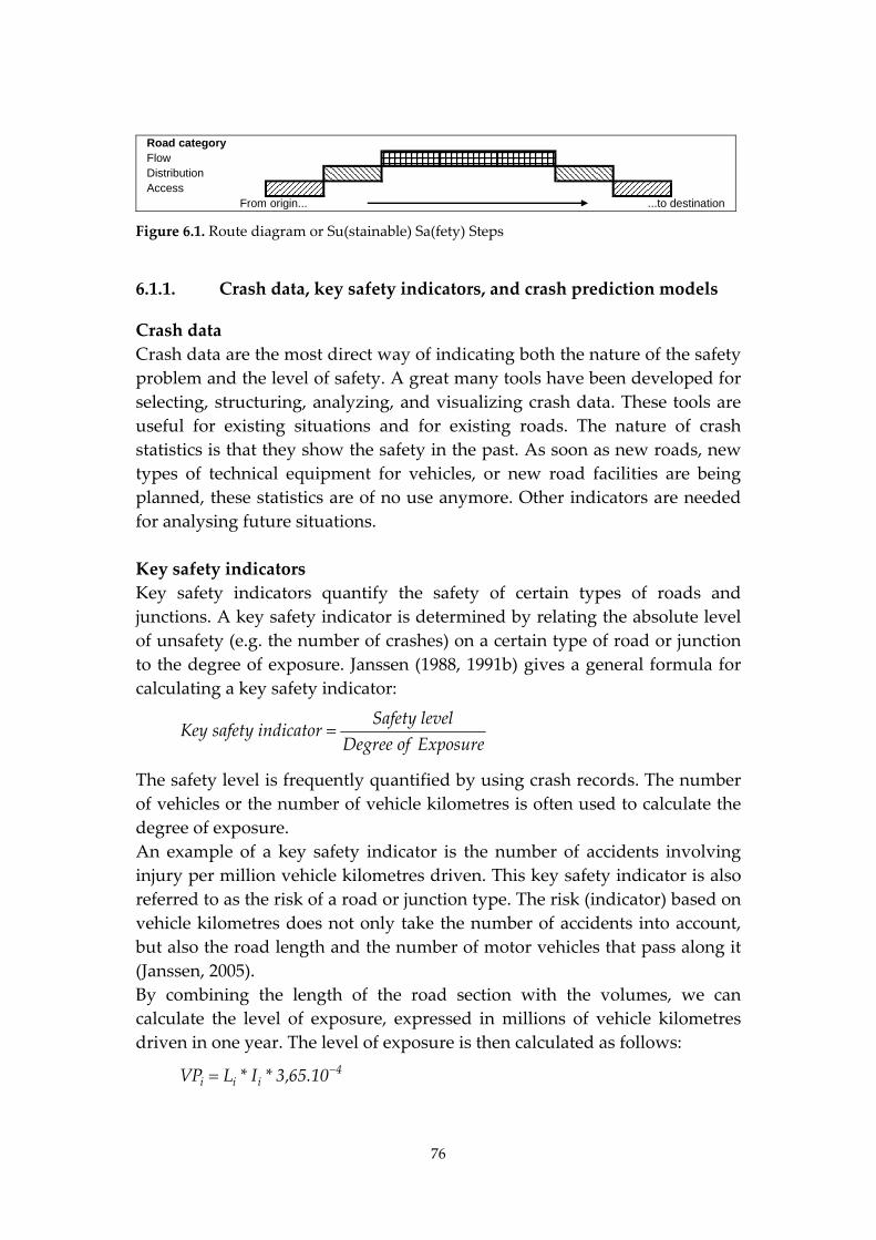
76
Road categoryFlowDistributionAccess
From origin... ...to destination
Figure 6.1. Route diagram or Su(stainable) Sa(fety) Steps
6.1.1. Crash data, key safety indicators, and crash prediction models
Crash data
Crash data are the most direct way of indicating both the nature of the safety
problem and the level of safety. A great many tools have been developed for
selecting, structuring, analyzing, and visualizing crash data. These tools are
useful for existing situations and for existing roads. The nature of crash
statistics is that they show the safety in the past. As soon as new roads, new
types of technical equipment for vehicles, or new road facilities are being
planned, these statistics are of no use anymore. Other indicators are needed
for analysing future situations.
Key safety indicators
Key safety indicators quantify the safety of certain types of roads and
junctions. A key safety indicator is determined by relating the absolute level
of unsafety (e.g. the number of crashes) on a certain type of road or junction
to the degree of exposure. Janssen (1988, 1991b) gives a general formula for
calculating a key safety indicator:
ExposureofDegree
levelSafetyindicatorsafetyKey
The safety level is frequently quantified by using crash records. The number
of vehicles or the number of vehicle kilometres is often used to calculate the
degree of exposure.
An example of a key safety indicator is the number of accidents involving
injury per million vehicle kilometres driven. This key safety indicator is also
referred to as the risk of a road or junction type. The risk (indicator) based on
vehicle kilometres does not only take the number of accidents into account,
but also the road length and the number of motor vehicles that pass along it
(Janssen, 2005).
By combining the length of the road section with the volumes, we can
calculate the level of exposure, expressed in millions of vehicle kilometres
driven in one year. The level of exposure is then calculated as follows:
4iii 10.65,3*I*LVP
77
in which VPi is the level of exposure of road section i in millions of vehicle
kilometres driven in one year, Li is the length of the road section i in km and
Ii is the daily volume for road section i.
Then, by multiplying the level of exposure VPi by the associated key
indicator Ki, the expected number of injury crashes LOi on road section i can
be estimated.
iii VP*KLO
The key indicator for road section i depends on the type of road. The typical
key safety indicators for road classes are presented in Section 3.1, Table 3.3
(Janssen, 1988 and 2005). These key safety indicators apply to crashes on both
the road sections and the intersections belonging to the road class. In this
way the intersections are appointed to the highest road class of two
intersecting classes; see Table 6.1
Intersecting road classes Higher class Lower class
Higher class to higher class to higher class
Lower class to higher class to lower class
Table 6.1. Appointing crashes on intersections to one of the intersecting road classes
The sum total of expected injury crashes on a route is derived by totalling the
expected injury crashes on the sections of the road classes that form part of
the route.
Application of key safety indicators
Traffic flow along the motorways in the Netherlands is gradually
diminishing because of increasing use and an almost unchanging capacity.
The accessibility of the economic centres is thus under heavy pressure.
Immers et al. (2001) presented a solution that, in the meantime, has become
known as ʹʹBypasses for accessibilityʺ. The main feature of this concept is the
introduction of an additional system of ʺunderlyingʺ main roads that can
handle a large part of regional traffic thus relieving the existing motorway
network. According to Immers et al. (2001), their application will result in a
considerable improvement of traffic flow and will contribute to a reduction
in the number of traffic casualties. However, Dijkstra & Hummel (2004) state
that a ʹbypasses networkʹ should also meet the requirements of a Sustainably
Safe Road Traffic.
78
Variant Road Type Description
Fatalities
(per billion
motor vehicle
kilometres)
In‐patients
(hospitalized)
(per billion
motor vehicle
kilometres)
Existing Road Types
MRN Motorway 2.61 24.14
SRN 80 Limited access, 1 x 2, 80 km/hour, at‐
grade junctions
10.11 124.25
SRN 100 Trunk Road, 1 x 2, 100 km/hour, at‐grade
junctions and grade‐separated junctions
8.76 81.39
Altered Road Types
MRN+ Motorway, extra lane 2.74 25.34
SRN+
(Bypasses)
2 x 2, narrowed, 70 km/hour, at‐grade
junctions and grade‐separated junctions
5.36 65.85
RTh
(SustainablySafe) Regional Through Road, 2 x 1, 100
km/hour, grade‐separated junctions
4.76 44.20
Table 6.2. Crash rates for various types of existing and altered roads
In a first elaboration, Immers et al. (2001) distinguished two alternatives: 1) a
motorway network with extra capacity through more lanes and 2) an
underlying main road network with greater capacity through more lanes and
sometimes split level intersections. Immers et al. used a mesoscopic
simulation model to find out the effects on traffic flow.
Dijkstra & Hummel (2004) compared the two bypasses network alternatives
with an option in which the underlying road network is designed as a
sustainably safe network (Table 6.2). This comparison shows that safety is
optimized in the sustainably safe option, but that it produces only a
relatively slight improvement in accessibility (Table 6.3). Although the
sustainably safe option has safe split‐level intersections, it only has a limited
capacity on road sections (one lane per direction). The opposite is true of the
bypasses alternatives; they have a greater amount of accessibility but have a
lower safety level. This is mainly because of the combination of larger
capacity (two lanes per direction) and (less safe) intersections at grade.
In this application of key safety indicators, it becomes obvious that
combining crashes on intersections and road sections in one indicator will
restrict the insight in the effects of new road classes. If the influence of the
intersection design is supposed to be large then the key safety indicator
should consider this. A second disadvantage of this application refers to the
type of simulation model used. The model only allows for considerations
79
concerning the capacity of the road sections. Again, the influence of the
intersection design is neglected.
Variant
MRN+ SRN+ Sustainably Safe
Vehicle minutes ‐19 ‐20 ‐12
Vehicle kilometres 5 3 2
Journey speeds 29 29 16
Number of fatalities 5 ‐4 ‐10
Number of in‐patients (hospitalized) 4 ‐2 ‐20
Energy use 5 1 1
Table 6.3. Effects of the different variants in percentages, in comparison to the present
situation (Source: Dijkstra & Hummel, 2004)
Measures aimed at influencing route choice should be evaluated by taking
into account the effects of intersection design on road safety and on traffic
flow.
Van der Sluis & Janssen (2000) evaluated three alternative networks for an
existing through‐road (a motorway) in the inner city of Maastricht (the
Netherlands). These alternative networks aimed at diverting the through‐
traffic from the inner city to routes which did not interact with the traffic.
Both the existing situation and the three alternative situations were modelled
in a macro simulation model (TRIPS). The model calculates the traffic
volumes for each road section. This output is used for the safety calculations.
The key safety indicators method is used for estimating the total number of
crashes in each alternative network. The differences between the alternative
networks, regarding the number of crashes, are very small. One of the
reasons for this result could be that the differences between the three
networks are also very small as far as road length and the actually adapted
road types are concerned. This type of evaluation needs differences between
alternatives large enough to result in relevant output. Differences between
crash figures will only be relevant and statistically significant for relatively
long stretches of road (a few kilometres).
Different route choices in various networks may be studied in various ways.
Simulation models are widely accepted as an evaluation instrument.
Wismans (2003) compared a great many existing models, gave criteria for
choosing models for evaluating route choice, and concluded that S‐Paramics
is a good tool for the purpose of route choice evaluation.
80
Figure 6.2. Test network in the micro‐simulation model S‐Paramics
In S‐Paramics an urban test network was set up (Figure 6.2), consisting of
nodes, links, and zones. Vehicles travel between zones. The test network
comprises three road types, Access, Distributor, and Through Roads, which
(in this test) only differ in speed limit: 30, 50, or 70 km/h respectively. The
Through Road, with an external zone on both sides, runs right through the
network. All traffic approaching this Through Road should give priority to
traffic on this through road. Vehicles that do not enter or leave the network
via these external zones always use the 30 km/h areas: these vehicles always
begin or end a route through the network on a 30 km/h road. Both the 4‐arm
intersections D, E, and F, and the 3‐arm intersections B, C, and H are priority
intersections.
The safety assessment, using route diagrams and simulated conflicts, can be
applied to every Origin‐Destination pair in the network. To illustrate this,
only the OD‐pair 2‐5 is considered (Figure 6.2). In this OD‐pair six possible
routes can be chosen:
1. Node A – B – C – F – H;
2. Node A – B – E – F – H;
3. Node A – B – E – G – H;
4. Node A – D – E – F – H;
5. Node A – D – E – G – H;
6. Node A – D – G – H.
81
In simulation I, the stochastic all‐or‐nothing assignment with a ʹperturbationʹ
factor 15 (percentage of link cost) is applied. In simulation II, the vehicles are
equipped with a route information system that advises on the up‐to‐date
situation on the network every minute. On the basis of this up‐to‐date
information, the model estimates the journey time for each vehicle and, at the
same time, determines the choice for a particular route. Simulation III
focused on the effects of a growing amount of external traffic on the route
choice of the internal traffic. For this reason the volume on the Through Road
was doubled. None of the roads in either of the three simulations reached
full capacity.
In the first simulation all vehicles chose route 2. In the second and third
simulations the vehicles are distributed along more routes. In simulation II,
39% chose route 2, 36% route 1, and 25% route 4. In simulation III, four
routes were followed: 60% chose route 2, 20% route 1, 13% route 6, and 7%
route 4.
The total number of crashes (during one hour) was calculated for each route,
using the key safety indicator method. When converting these hourly
numbers to the number of accidents per year, we find a crash level varying
between 0.2 to 0.6 crashes. The crash level of route 3 is highest in every
simulation. Given the key safety indicator method, higher volumes on a
route (in this case route 3) will result into more crashes. The key safety
indicator approach functioned quite well in this application because the
intersections did not change but only the volumes did.
Crash Prediction Models
Crash Prediction Models are another way of indicating road safety. Using
Average Annual Daily Traffic and road characteristics as an input, the
number of crashes or casualties can be calculated (FHWA, 2000, 2005;
Reurings et al., 2006).
The general formula for a crash prediction model is:
,eAADT ijj xii
where μ is the expected number of crashes in a certain period, AADT is the
Annual Average Daily Traffic in the same period, xj are other explanatory
variables, α, β, γj are the parameters to be estimated and the subscript i
denotes the value of a variable for the i‐th road section.
Reurings et al. (2006) conclude that for main rural roads the other
explanatory variables should at least include section length, number of exits,
carriageway width, and shoulder width. This type of model can be used for
82
either intersections or road sections; a combined model for the route level has
not been developed yet.
6.1.2. Traffic conflicts and surrogate safety measures
Road safety on the level of road sections and junctions is mostly expressed as
the number of crashes or casualties. However, these numbers are usually too
small to allow for an in‐depth analysis of separate road sections or junctions.
Therefore, safety indicators have been developed that have a direct or
indirect relationship with crashes. This section will describe the most
important safety indicators.
Traffic conflicts
The number of traffic conflicts and near‐crashes is much higher than the
number of crashes or casualties. They are, therefore, more suitable for
analysis. Studying conflicts and near‐crashes presumes a relationship
between a conflict and a ʹrealʹ crash. This relationship was studied
extensively by Hydén (1987) and Svensson (1998). In Germany, Erke et al.
(1978) and Zimolong (1982) gave a first overview. Subsequently, Perkins &
Harris (1968) started using conflict analysing techniques. Erke et al. ﴾1985﴿ compiled a handbook.
The assumption underlying this method is that situations with a large
number of conflicts have a higher probability for accidents. Trained
observers interpret traffic situations, count the number of (serious) conflicts,
and analyse these conflicts. Conflicts are actions by road users, which may
lead to problems (e.g. late braking, cutting of bends) and which have a high
frequency. Several measurements have been proposed to characterize traffic
conflicts in detail. For example time to collision (TTC), deceleration rate (DR),
encroachment time (ET), post encroachment time (PET), etc. are used to
determine the severity of a traffic conflict objectively. ﴾PIARC, 2004). This technique enlarges the amount of data but the used parameters resulting
from the manoeuvres are not necessarily direct indicators of accident risk
and accident severity.
Surrogate safety measures
Surrogate safety measures in general are measures indicating aspects of road
user behaviour that are related to road safety. Well‐known examples of these
measures are driving speed, red‐light running, headway, overtaking, and
giving right of way. In addition to these real‐life indicators, safety measures
have been developed for microscopic simulation models. When using a
microscopic model conflicts between vehicles will be an integral part of the
83
simulation. A microscopic model uses a set of internal models for simulating
driver behaviour. These behavioural models are usually calibrated by using
observations of car drivers in several conditions. This thesis will not go into
these internal models, and will treat these as black boxes.
The Time To Collision (TTC) is an indicator for the seriousness of a traffic
conflict. A traffic conflict is defined by FHWA (2003) as ʺan observable
situation in which two or more road users approach each other in time and
space to such an extent that there is a risk of collision if their movements
remain unchanged.ʺ The TTC value differs for junctions and road sections. A
TTC on road sections will only be relevant when one vehicle is following
another one. A vehicle on a road section can only have one TTC value. A
TTC value on junctions relates to vehicles approaching each other on two
different links. A vehicle approaching a junction can have more than one
TTC value, depending on the number of vehicles on the other links.
Minderhoud and Bovy (2001) have developed two indicators that can be
applied in micro‐simulation models and are based on the TTC: the Time
Exposed TTC (TExT) and the Time Integrated TTC (TInT). The TExT
expresses the duration that the TTC of a vehicle has been below a critical
value ‐ TTC* ‐ during a particular period of time. The TExT is thus the sum of
the moments that a vehicle has a TTC below the TTC* (Figure 6.3). That
means that the smaller the TExT, the shorter time a vehicle is involved in a
conflict situation, and therefore, the safer the traffic situation is. The TExT
indicator does not express the extent to which TTC values occur that are
lower than the critical value. In order to include the impact of the TTC value,
the TInT indicator has been developed. This is the area between TTC* and
the TTC that occurs (Figure 6.3).
Figure 6.3. Safety indicators in a micro‐simulation model according to Minderhoud
& Bovy (2001)
84
The impact of a conflict may also be expressed by calculating the potential
collision energy (PCE) that is released when the vehicles are in conflict and
collide with each other. Masses and speeds of the vehicles, as well as the way
in which the vehicles collide with each other, i.e. the conflict type, influence
the potential collision energy.
The outcome of these conflict analyses will be used to compare the types of
conflicts in a given simulation with the types of conflicts being ʹacceptableʹ in
a Sustainably Safe road environment, (e.g. conflicts with opposing vehicles
should be minimised at high speed differentials).
Dijkstra et al. (2007) have applied these types of indicators in a test network
(Figure 6.2). Three simulations (I, II, and III in Section 6.1.1) were used to
compare the outcome for the indicators. They divided the value of each
indicator by the number of vehicles on a route, in order to get indicator
ratios. The four ratios (for the number of conflicts, TExT, TInT and PCE) do
appear to differ from each other. The ratio for the number of conflicts
depends on the amount of traffic in the network: the more traffic, the more
conflicts. The TET ratio values are also subject to the volumes in the network:
the more traffic, the more exposure to conflicts. The changes in the three
consecutive simulations apparently do not influence the scores of TExT ratio
very much. This is not true for the TInT ratio values, which show many
changes between the simulations. Furthermore, the levels of the TInT ratio
values do not change when the volumes go up. The TInT ratio is very much
influenced by the nature (seriousness) of the interactions between vehicles,
not by the amount. The differences between the simulations are not
specifically focused on changing this nature.
Finally, the PCE ratio values are much higher in the third simulation (with
more traffic on the central main road) than in the other two simulations. That
is because of both more traffic on this road and higher driving speeds,
resulting in potentially more collision energy in each conflict.
Each of the conflict indicators appears to have its own surplus value for
assessing the safety of routes in a network. More research is needed to find
out the pros and cons of using these kinds of indicators in networks that are
more complex.
6.1.3. Qualitative safety assessment
In a qualitative safety assessment, existing or planned road infrastructure is
examined to find out the safety conditions. This can be done either by
comparing the infrastructure to a sort of ideal situation or by giving an
expert opinion.
85
Comparing design features to design requirements: road sections and
intersections
In the Netherlands, the concept ʹSustainably‐Safe trafficʹ (Koornstra et al.,
1992; Wegman & Aarts, 2006) is the leading concept for road safety policy
and research. The main goal of a Sustainably‐Safe road transport system is
that, in thirty years time, only a fraction of the annual number of road
accident casualties would remain.
It is of great importance for a Sustainably‐Safe traffic system that, for each of
the different road categories, road users know what behaviour is required of
them and what behaviour they may expect from other road users. Their
expectations should be supported by optimising the recognition of the road
categories.
The three main principles in a Sustainably‐Safe traffic system are:
functionality,
homogeneity,
recognition/predictability.
The functionality of the traffic system is important to ensure that the actual
use of the roads is in accordance with the intended use. This principle led to
a road network with only three categories: through roads, distributor roads,
and access roads. Each road or street may only have one function; for
example, a distributor road cannot have any direct dwelling access. The
speed limit is an important characteristic of each road category: access roads
have low speed limits (30 km/h in urban areas and 60 km/h in rural areas)
while through roads have speed limits of 100 or 120 km/h.
The homogeneity is intended to avoid large speed, direction, and mass
differences by separating traffic types and, if that is not possible or desirable,
by making motorised traffic drive slowly.
The third principle is that of the predictability of traffic situations. The design
of the road and its environment should promote recognition, and therefore
the predictability, of any possible occurring traffic situation.
The three principles have been translated into safety design requirements, for
instance:
For road sections
Avoiding conflicts with oncoming traffic
Avoiding conflicts with crossing traffic
Separating different vehicle types
Avoiding obstacles along the carriageway
86
For junctions
Avoiding conflicts with crossing traffic
Reducing speed
Limiting the number of different traffic facilities
Design requirements in general, which are part of design manuals, are not
only based on safety arguments but also on other arguments, like capacity
and liveability. In addition a designer will apply the requirements given the
constraints in a real‐life situation. Therefore, Van der Kooi & Dijkstra (2000)
suggested a test to find out the differences between the original safety
requirements and the characteristics of the actual design features. This
Sustainable Safety Test systematically compares each design element or
feature with the relevant safety requirements. The correspondence of a
design element to a requirement is expressed by a percentage (of the road
length). The total score of a design on Sustainable Safety is the average of
these percentages.
Comparing design features to design requirements: routes
Very little attention has been paid to the consequences of the functional
requirements, i.e. the route choice issues (Hummel, 2001). The present study
is directed towards the analysis of the mechanisms behind route choice and
route management measures, such as route information systems (roadside
and in‐vehicle) and speed limits of different road categories.
Sustainably‐Safe aims to incorporate road safety in transportation planning.
In the planning phase one needs to determine whether the network will
function according to the preceding network requirements, especially
regarding safety. It is difficult to review the consequences of a traffic plan
because of the large amount of data that plays a role in such plans. That is
why planners often use traffic models and simulation models. The classic
traffic models assign the total traffic volume to the road sections of the
different networks. An example of the application of such a model to the
mesh of the main road network is given in Immers et al. (2001). In micro‐
simulation models, however, it is possible to allow separate vehicles to
follow a route through a network. The route choice of every simulated
vehicle depends on a number of previously established conditions and on
several variables that are functions of: in‐vehicle equipment, facilities along
the road, the driverʹs motive, time of day, and interaction with the rest of the
traffic. In this way, it is possible to determine in advance how route choice
changes if facilities are planned along the road, or in‐vehicle. AVV (2002) and
Wismans (2003) give a general overview of the features and use of simulation
87
models. Hidas (2005) compares three frequently used models: AIMSUN,
VISSIM and Paramics.
Morsink et al. (2004) used a micro‐simulation model for an urban network to
study which consequences occur by adapting the current speed limits per
road type. The main ingredients for the analysis of route choice by dynamic
microscopic modelling are: an efficient model of a representative road
network, features for modelling route choice behaviour, and indicators for
traffic safety and network performance.
The route choice analysis reference case is the 1997 Utrecht traffic situation
focusing on the morning rush‐hour between 07.00h and 10.00h. In this
period, 230,000 vehicles were involved, with the 7.45h to 8.45h time interval
as the busiest hour.
For modification of the reference case, measures were applied at road
network level to increase route resistance defined by travel time. For this
purpose, the maximum speed on distributor and access roads was lowered in
three cases according to Table 6.4. No other modifications were made to the
model or simulation procedure for these cases. This means that the dynamic
OD‐matrices were unaltered and the effects of the modification of maximum
speeds concerning modal split and departure time were not taken into
account.
Access roads Distributors Cases
Urban Rural Urban Rural
Reference case 50 50 50 80
Case 1 30 50 50 80
Case 2 30 30 30 80
Case 3 20 50 40 80
Table 6.4. Modification of speed limits (km/h) on access roads and distributors for
three cases; speed limits on through roads (100 or 120 km/h) remained unchanged
These cases were selected on the basis of the following hypothesis per case:
Case 1: driving on urban access roads will be minimized and driving on
distributors and flow roads will be stimulated.
Case 2: driving on through (flow) roads will be stimulated, without making
a distinction between access and (urban) distributors.
Case 3: driving on through roads will be stimulated and driving on
distributors will be stimulated in favour of access roads.
88
The total number of vehicle kilometres did not show significant changes for
the modified cases (Table 6.5). The urban access roads show fewer vehicle
kilometres in all cases because of their lower attractiveness (higher
resistance). The urban distributors in case 2 have fewer vehicle kilometres
because these roads were as attractive (or unattractive) as access roads.
Absolute values Reference Case 1 Case 2 Case 3
Vehicle hours 52,540 100 106 131 122
Vehicle kilometres 1,761,938 100 100 101 101
Vehicle kilometres per road category
Absolute values Reference Case 1 Case 2 Case 3
Through (flow) road 990,869 100 100 103 102
Distributors, rural 324,234 100 101 105 104
Distributors, urban 314,102 100 107 92 105
Access road, rural 950 100 100 100 100
Access road, urban 131,782 100 80 98 75
Total 1,761,938 100 100 101 101
Table 6.5. Quantitative overview of network performance of the modified cases with
respect to the reference case
This study by Morsink et al. shows that comparing an existing situation to an
ideal situation can be done on a network level by using a simulation model.
In doing so, the comparison even gains a quantitative nature, given the
assumption that the ideal situation (the system of speed limits) is the safest
situation.
Expert judgement
The main objective of safety audits is to ensure that highway schemes
operate as safely as possible, i.e. to minimise the number and severity of
occurring accidents. This can be achieved by avoiding accident prone
elements and by providing suitable accident reducing elements. The purpose
of safety audits is to ensure that ‘mistakes’ are not built into new schemes.
The UK definition is as follows: A formal procedure for assessing accident
potential and safety performance in the provision of new road schemes, and
schemes for the improvement and maintenance of existing roads (IHT, 1996).
Safety audits can be applied in schemes of various types. Such schemes
generally fall into the following categories:
89
major highway schemes;
minor improvements;
traffic management schemes;
development schemes;
maintenance works.
The auditor should be a road safety expert, preferably working as part of an
audit team. During an audit, checklists can be used. A set of checklists is
usually available, consisting of specific checklists for each road type.
Whether this type of expert judgement will have an impact on the reduction
of the number of crashes is still subject to research. Estimations of the effect
of a safety audit are in the order of a few percent points (SWOV, 2009b).
6.1.4. Selection of methodologies with respect to the route level
Crash data can be used for existing roads and streets, given the past history of
road users and vehicles. Planned or newly built road sections have no
accident history, and neither do traffic situations with vehicles equipped
with experimental ADAS systems. Therefore, accident data will be used only
as a reference for the safety level of existing situations.
Key safety indicators can be used for evaluating new roads and streets. This
method shows the total number of crashes on a road type, or on a road
section. It does not show the number of crashes for a specific route choice.
This type of indicator only takes into account one kind of change caused by
ADAS: the sum of route choice behaviour for all users (resulting from
changes in traffic flows, which are input for the indicator).
Crash prediction models are of the same nature as key safety indicators. The
additional value of crash prediction models is that these can be more detailed
regarding road and traffic characteristics than crash safety indicators.
Nevertheless, crash prediction models do not incorporate characteristics
about vehicles with and without ADAS.
Comparing design features to design requirements is above all useful for
designers to check their designs in a preliminary stage. This method may
also be used when modelling road networks. Both features and requirements
may be varied. The method may be applied to road sections and intersections
separately and to strings of road sections like routes.
Traffic conflicts may be used in a method for studying specific safety
problems at a few locations, mostly intersections. The method requires a high
90
level of expertise for the observers, and takes quite a lot of time (a few days)
for each location. The method is particularly useful for individual locations.
Surrogate (safety) measures have been developed to be used in micro‐
simulation models. These measures are calculated for each vehicle
separately. In this way the safety of each vehicle route can be computed.
Expert judgement is mostly used for safety assessment of either new road
schemes or new ADAS. Applying this method to routes would be a new way
of safety auditing.
Conclusions
From the list of methods, it can be concluded that a few methods are suited
for studying road safety effects of changes in the use of the road network,
caused by adaptations of the network structure and/or road classification.
The effects of these changes on route choice, in particular, determine the
choice of method. The methods are key safety indicators, crash prediction
models, comparing features to requirements, and surrogate safety measures.
Only surrogate safety measures will show output for the safety of individual
routes.
6.2. Route criteria, route scores and route stars
On the route level one can compare design features to design requirements
according to the concept of the Sustainable Safety concept. This concept
comprises functional requirements which can be focused on the route level.
The most important requirement for trips is: the shortest and safest route
should coincide. In order to test this requirement more detailed safety criteria
were developed. These criteria are determined for all routes belonging to one
OD‐pair. Next a safety score for each route and for each OD‐pair will be
introduced. Finally, the safety score for a set of OD‐pairs is formulated.
Route criteria, route diagrams and route stars are indicators of the safety of
routes in a road network. They can be applied when assessing effects of
changes in a road network, e.g. when adding new trip generating areas to an
existing urban area or when inserting a new road section to the network.
These major changes to a network will in their turn change a great many
routes, and will therefore also affect road safety. The methods described
show, which routes will be safest, and which of these routes will attract most
of the traffic.
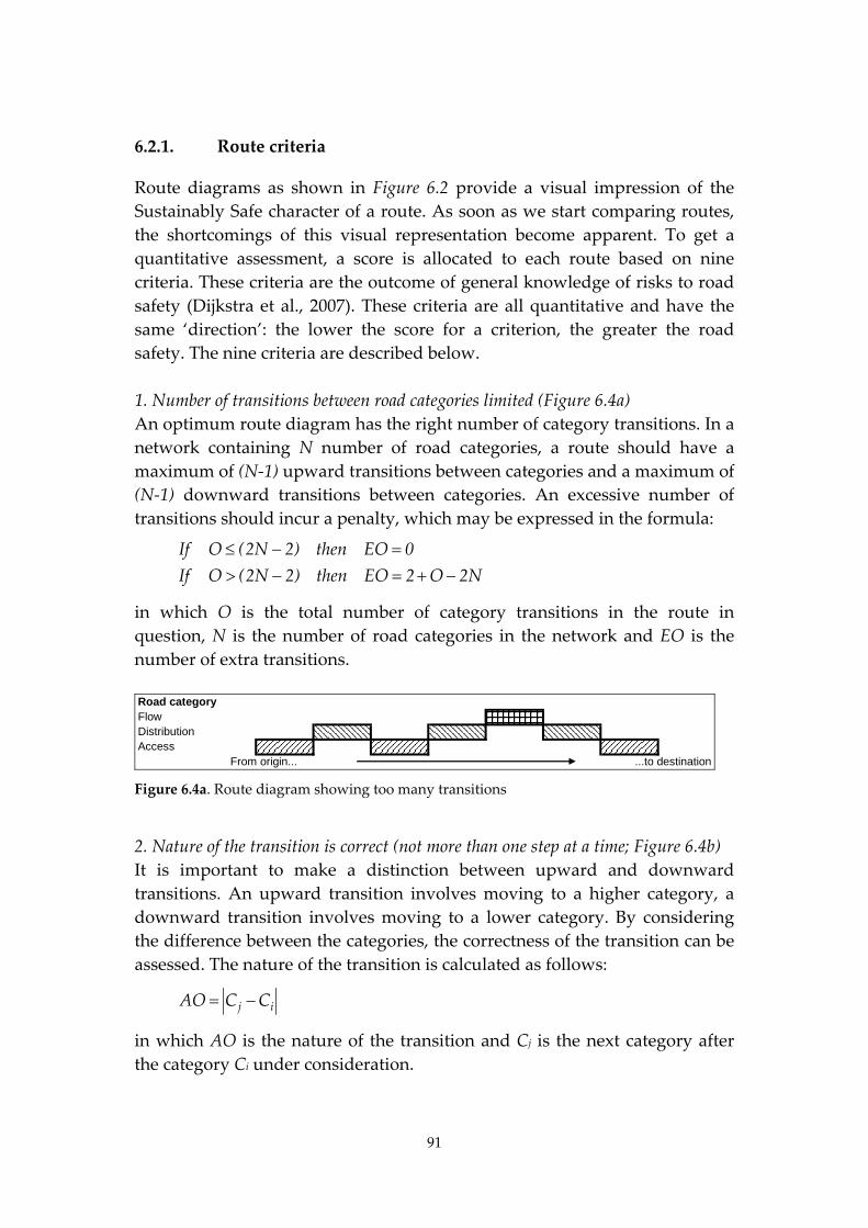
91
6.2.1. Route criteria
Route diagrams as shown in Figure 6.2 provide a visual impression of the
Sustainably Safe character of a route. As soon as we start comparing routes,
the shortcomings of this visual representation become apparent. To get a
quantitative assessment, a score is allocated to each route based on nine
criteria. These criteria are the outcome of general knowledge of risks to road
safety (Dijkstra et al., 2007). These criteria are all quantitative and have the
same ‘direction’: the lower the score for a criterion, the greater the road
safety. The nine criteria are described below.
1. Number of transitions between road categories limited (Figure 6.4a)
An optimum route diagram has the right number of category transitions. In a
network containing N number of road categories, a route should have a
maximum of (N‐1) upward transitions between categories and a maximum of
(N‐1) downward transitions between categories. An excessive number of
transitions should incur a penalty, which may be expressed in the formula:
N2O2EOthen)2N2(OIf
0EOthen)2N2(OIf
in which O is the total number of category transitions in the route in
question, N is the number of road categories in the network and EO is the
number of extra transitions.
Road categoryFlowDistributionAccess
From origin... ...to destination
Figure 6.4a. Route diagram showing too many transitions
2. Nature of the transition is correct (not more than one step at a time; Figure 6.4b)
It is important to make a distinction between upward and downward
transitions. An upward transition involves moving to a higher category, a
downward transition involves moving to a lower category. By considering
the difference between the categories, the correctness of the transition can be
assessed. The nature of the transition is calculated as follows:
ij CCAO
in which AO is the nature of the transition and Cj is the next category after
the category Ci under consideration.
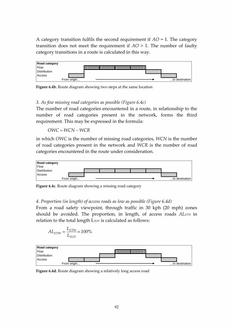
92
A category transition fulfils the second requirement if AO = 1. The category
transition does not meet the requirement if AO > 1. The number of faulty
category transitions in a route is calculated in this way.
Road categoryFlowDistributionAccess
From origin... ...to destination
Figure 6.4b. Route diagram showing two steps at the same location
3. As few missing road categories as possible (Figure 6.4c)
The number of road categories encountered in a route, in relationship to the
number of road categories present in the network, forms the third
requirement. This may be expressed in the formula:
WCRWCNOWC
in which OWC is the number of missing road categories, WCN is the number
of road categories present in the network and WCR is the number of road
categories encountered in the route under consideration.
Road categoryFlowDistributionAccess
From origin... ...to destination
Figure 6.4c. Route diagram showing a missing road category
4. Proportion (in length) of access roads as low as possible (Figure 6.4d)
From a road safety viewpoint, through traffic in 30 kph (20 mph) zones
should be avoided. The proportion, in length, of access roads ALETW in
relation to the total length LTOT is calculated as follows:
%100L
LAL
TOT
ETWETW
Road categoryFlowDistributionAccess
From origin... ...to destination
Figure 6.4d. Route diagram showing a relatively long access road
93
5. Proportion (in length) of distributor roads as low as possible (Figure 6.4e)
Distributor roads are the least safe when it comes to the accident risk. For
that reason, the ratio in length of these roads should be kept as low as
possible. The proportion, in length, of distributor roads ALGOW in relation to
the total length LTOT is calculated as follows:
%100L
LAL
TOT
GOWGOW
Road categoryFlowDistributionAccess
From origin... ...to destination
Figure 6.4e. Route diagram showing a relatively long distributor road
6. Travel distance
The smaller the total distance LTOT travelled on a route, the less risk to which
a vehicle is exposed. The total distance LTOT is equal to the sum of the
distance over access roads LETW, the distance over distributor roads LGOW and
the distance over through roads LSW. This is expressed as the formula:
SWGOWETWTOT LLLL
7. Travel time
The total travel time R is calculated for each route on the basis of an empty
network. This is done by totalling the length of the categories divided by
their respective speed limits, expressed by the formula:
SW
SW
GOW
GOW
ETW
ETW
V
L
V
L
V
LR
Travel time can also be derived from a simulation model. However, this will
make this criterion very dynamic, and hard to interpret. This argument also
holds for a criterion called ʹloss timeʹ, based on subtracting the minimal
travel time (empty network) from the real travel time (from the model).
8. As few turnings as possible across oncoming traffic
The number of left turns (LAB) at junctions can be recorded for each route.
Because turning left is seen as the most dangerous manoeuvre (Drolenga,
2005), the score declines as the number of these movements increases.
94
9. Low junction density on distributor road
The purpose of this requirement is to assess the route’s potential for
disruption on the distributor roads within it. The junction density KPD is
defined as the number of junctions on distributor roads K per km of
distributor road. This is expressed as the formula:
GOWL
KKPD
Nine criteria summarised
The nine criteria including their dimensions are shown in Table 6.6.
Most of these criteria are related to each other. Criteria 1 to 5 are closely
related to each other because they are the quantitative description of the
route diagram. These five criteria should preferably be applied together, in
order to be sure that the route fulfils the aims of Sustainable Safety. Travel
distance is related to travel time in an ʹemptyʹ network. As soon as the
network is saturated, this relationship will disappear. The proportion of a
certain road category and travel distance seem to be mutually dependent,
however, two routes having the same length of access roads will have
different proportions of access roads when the total travel distances of both
routes differ.
Criterion Description Unit
1 Number of transitions Number of additional transitions
2 Nature of transitions Number of wrong transitions
3 Missing road categories Number of missing categories
4 Proportion of access roads Percentage of total distance
5 Proportion of distributors Percentage of total distance
6 Travel distance Meters
7 Travel time Seconds
8 Left turns Number of left turns
9 Junction density Number of junctions per kilometre
Table 6.6. Nine criteria for route diagrams
95
6.2.2. Route scores and stars
Sustainable Safety Score
For each route we calculate the scores for the nine aforementioned criteria by
collecting the data and applying the formulae. Using a multi‐criteria analysis,
we then try to arrange alternative routes in order of preference.
Standardisation of the criterion scores is necessary if the different scores of
the various routes are to be compared. The scores are standardised on the
basis of interval standardisation. This means that the best alternative is
awarded a score of 0, the worst a score of 1, and the other options are scaled
between 0 and 1. This is done by reducing the score by the lowest score for
the criterion in question and dividing this difference by the difference
between the maximum score and the minimum score for the criterion in
question. This is expressed as the formula:
}C{min}C{max
}C{minCG
jijjij
jijjiji
in which Gji is the standardised score of alternative i for criterion j and Cji is
the criterion score of alternative i for criterion j.
In determining the minimum and maximum scores for a criterion, not only
the routes that are actually followed should be taken into account, but also
the routes that are not followed but are nevertheless available in the
infrastructure.
Routes can easily be compared by using stars to visually represent the
standardised scores for the nine criteria. The nine points of the star represent
the nine criteria. Each point shows ʹ1 ‐ Gji ʹ: the longer a point, the better the
score for this route is in relationship to alternative routes. This means that the
more complete the star is, the more sustainably safe the route is. The scores
for the nine criteria on two routes are shown as an example in Figure 6.5.
Figure 6.5. Examples of route stars for two routes
-0.2
0
0.2
0.4
0.6
0.8
1
Number of transitions
Nature of transitions
Missing categories
% Access roads
% DistributorsDistance
Time
Left turns
Intersection density
-0.2
0
0.2
0.4
0.6
0.8
1
Nature of transitions
Missing
categories
% Access roads
% Distributors Distance
Time
Left turns
Intersection
density
Number of
transitions
96
If a star is nearly complete for criteria 1 to 5 (starting at the ʹ12 oʹclockʹ
arrow), this implicates that the route diagram will also be according to the
Sustainable Safety criteria.
The left‐hand route (purple star) has the worst score for the first requirement
(the number of additional transitions) because no point, or only part of a
point, is visible. By contrast, the right‐hand route (green star) has the best
score for this requirement because the entire point is visible. Because the
green star is more complete than the purple star, it may be concluded that
the right‐hand route fulfils the requirements of the Sustainable Safety policy
more than the left‐hand route.
Criteria weights
After the scores have been standardised, the weighting of the criteria can be
determined. If each criterion is determined to be of equal importance, then
each of them has the same weight. If one or more criteria are considered
more important, these may be allocated a greater weight than less important
criteria. The sum of the weights of the criteria must always come to 1, so if all
nine criteria are considered of equal importance, each criterion is given a
weight of 1/9.
Total score for a route
To arrive at a total score for each route, the standardised score is multiplied
by the weight and added up over the nine criteria to give total scores
(weighted totalling method). The outcome of this total score indicates the
degree of unsafety. To arrive at a safety score, the unsafety score is deducted
from 1 and multiplied by 100% so that the safety score will fall between 0
and 100%. This is expressed as the formula:
C
1cccr gss100100VV (6.1)
in which VVr is the safety score of route r, C is the number of criteria, ssc is the
standardised score for criterion c and gc is the weight of criterion c.
Sustainable Safety Level OD‐relationship
Using the calculated safety scores of the various routes that are associated
with an OD relationship and distribution of the vehicles over these routes,
we calculate the safety level of a OD relationship. In doing so, it is important
to also include the safety level of routes that are not selected (in this
simulation). After all, traffic may well follow these routes in a subsequent
simulation.
97
Distribution of vehicles over routes
The distribution of vehicles over the routes per OD relationship is indicated
by calculating the percentage of the total number of vehicles per OD
relationship that travel via route r. This is expressed by the formula:
%100I
IV
OD
rr,OD (6.2)
in which VOD,r is the percentage of vehicles that travel via route r from origin
H to destination B , Ir is the absolute number of vehicles that travel via route r
and IOD is the total number of vehicles that travel from origin H to
destination B.
Safety level OD
The unsafety score for each route is multiplied by the percentage distribution
of the vehicles following this route, and then added up over the various
routes to give a total score for an OD relationship. The outcome of this total
score indicates the degree of unsafety of the OD relationship. To arrive at a
safety score, the unsafety score is deducted from 1 and multiplied by 100%,
so that the safety score will fall between 0 and 100%. This is expressed by the
formula:
R
1r
r,ODrOD
100
V)VV100(100VV
or, in a more simple formula:
R
1r
r,ODrOD
100
VVVVV (6.3)
in which VVOD is the safety score of OD relationship OD, R is the number of
routes associated with OD relationship OD, VVr is the safety score of route r,
calculated using formula Y.2.10, and VOD,r is the percentage of vehicles that
travel via route r from origin H to destination B, (Formula 6.2).
Sustainable Safety Level of OD‐relationship given the infrastructure
In the Sustainable Safety Level of an OD relationship, discussed above, both
route choice and infrastructural characteristics of the routes are given factors.
Improvements in the infrastructural characteristics may increase the
Sustainable Safety level, as may another choice of route. In order to separate
these two effects, which are probably interdependent, we introduce the
Sustainable Safety Level of an OD relationship given the (existing)
infrastructure. In doing so, we ignore the infrastructural inadequacies of the
98
routes. This gives us more insight into the safety benefits that may be
achieved by influencing the route choice of vehicles.
The safest route in an OD relationship, which does not have to have a safety
level of 100 by definition, is standardised to the value of 100 and the least
safe route is standardised to the value of 0. If all vehicles make use of the
safest route, the safety level of the OD relationship under consideration is 100
given the infrastructure and no more progress can be achieved by influencing
route choice. If all vehicles make use of the least safe route, the safety level of
the OD relation under consideration is equal to 0 given the infrastructure.
The standardised road safety score of a route r may be defined as follows:
%100}VV{min}VV{max
}VV{minVVVV
rrrr
rrrrs
By entering the standardised safety score of a route VVrs instead of the non‐
standardised safety score VVr , it is possible to define the safety score of an
OD given the infrastructure as follows:
R
1r
r,ODrsOD
100
VVVVV (6.4)
6.3. Retrieving conflicts from micro‐simulation models
The definition of TTC is ʺthe time to a collision with a vehicle that is in front
(on road sections) or conflicting (on junctions) if neither vehicle changes its
course or speedʺ. The TTC is an indicator for a traffic conflict and is therefore
related to the crash risk. Low TTCs mean a higher crash risk and high TTCs
mean a lower crash risk.
On a junction, the TTC is calculated on the basis of one or more vehicles
coming from another arm of the junction. In addition, a vehicle on a road
section can only have one TTC at any given time but on a junction a vehicle
can have multiple TTCs simultaneously.
The border line between the end of a road section and the beginning of a
junction is determined by the safe stopping distance, referred to henceforth
and in the formulae as SSD. The SSD for a vehicle i on road section j is
defined as:
i2
2j
ij
ijA6.32
Vrt
6.3
VSSD (6.5)
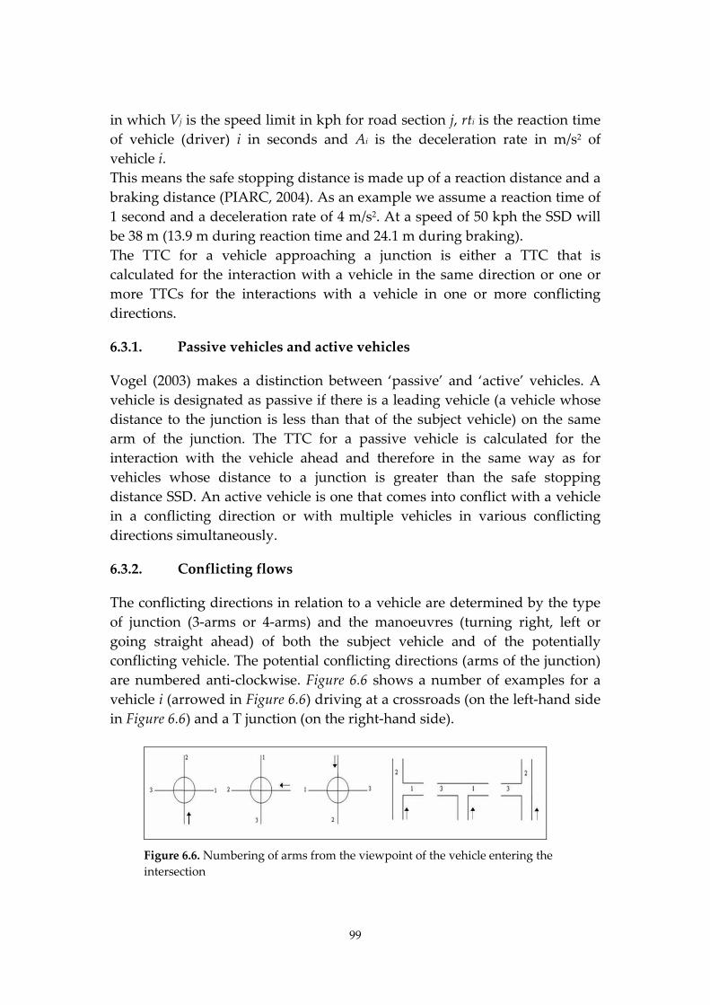
99
in which Vj is the speed limit in kph for road section j, rti is the reaction time
of vehicle (driver) i in seconds and Ai is the deceleration rate in m/s2 of
vehicle i.
This means the safe stopping distance is made up of a reaction distance and a
braking distance (PIARC, 2004). As an example we assume a reaction time of
1 second and a deceleration rate of 4 m/s2. At a speed of 50 kph the SSD will
be 38 m (13.9 m during reaction time and 24.1 m during braking).
The TTC for a vehicle approaching a junction is either a TTC that is
calculated for the interaction with a vehicle in the same direction or one or
more TTCs for the interactions with a vehicle in one or more conflicting
directions.
6.3.1. Passive vehicles and active vehicles
Vogel (2003) makes a distinction between ‘passive’ and ‘active’ vehicles. A
vehicle is designated as passive if there is a leading vehicle (a vehicle whose
distance to the junction is less than that of the subject vehicle) on the same
arm of the junction. The TTC for a passive vehicle is calculated for the
interaction with the vehicle ahead and therefore in the same way as for
vehicles whose distance to a junction is greater than the safe stopping
distance SSD. An active vehicle is one that comes into conflict with a vehicle
in a conflicting direction or with multiple vehicles in various conflicting
directions simultaneously.
6.3.2. Conflicting flows
The conflicting directions in relation to a vehicle are determined by the type
of junction (3‐arms or 4‐arms) and the manoeuvres (turning right, left or
going straight ahead) of both the subject vehicle and of the potentially
conflicting vehicle. The potential conflicting directions (arms of the junction)
are numbered anti‐clockwise. Figure 6.6 shows a number of examples for a
vehicle i (arrowed in Figure 6.6) driving at a crossroads (on the left‐hand side
in Figure 6.6) and a T junction (on the right‐hand side).
Figure 6.6. Numbering of arms from the viewpoint of the vehicle entering the
intersection
100
6.3.3. Time required to conflict zone
Per time step t, the time required by both active vehicles to reach the conflict
zone is estimated by dividing the distance to the conflict zone by the speed
(the dimensions of the conflict zone are determined by the width of both
vehicles). This is expressed as the formula below (Van der Horst, 1990):
)t(V
)t(d)t(AT
i
ii
in which ATi is the time required by vehicle i to reach the conflict zone at
point in time t, di is the distance to the conflict zone at point in time t and Vi is
the speed at point in time t.
6.3.4. First vehicle
Using the estimated arrival times per step in time, it is possible to calculate
which vehicle will arrive at the conflict zone first; this is the vehicle with the
lowest AT as calculated with the formula given above. The vehicle that will
arrive first is designated vehicle i and the second vehicle is designated
vehicle k.
6.3.5. Clearance time
For the vehicle that will arrive first (vehicle i), the time required to leave the
conflict zone is calculated. This required time is the difference between the
moment when the vehicle is estimated to enter the conflict zone (ATi) and the
moment when the vehicle is estimated to leave the conflict zone. The
required clearance time TO for vehicle i at point in time t is equal to:
)t(V
bl)t(TO
i
kii
in which li is the length of vehicle i, bk is the width of vehicle k and Vi(t) is the
speed of vehicle i at point in time t.
This formula may be used for all converging conflicts. In some types of
conflict this formula is also valid, for example, in a frontal conflict both
vehicles could hit each other at a very small angle.
6.3.6. Collision course
Active vehicles are on a collision course if the difference between the arrival
times of the two vehicles i and k is less than the required clearance time of
vehicle i:
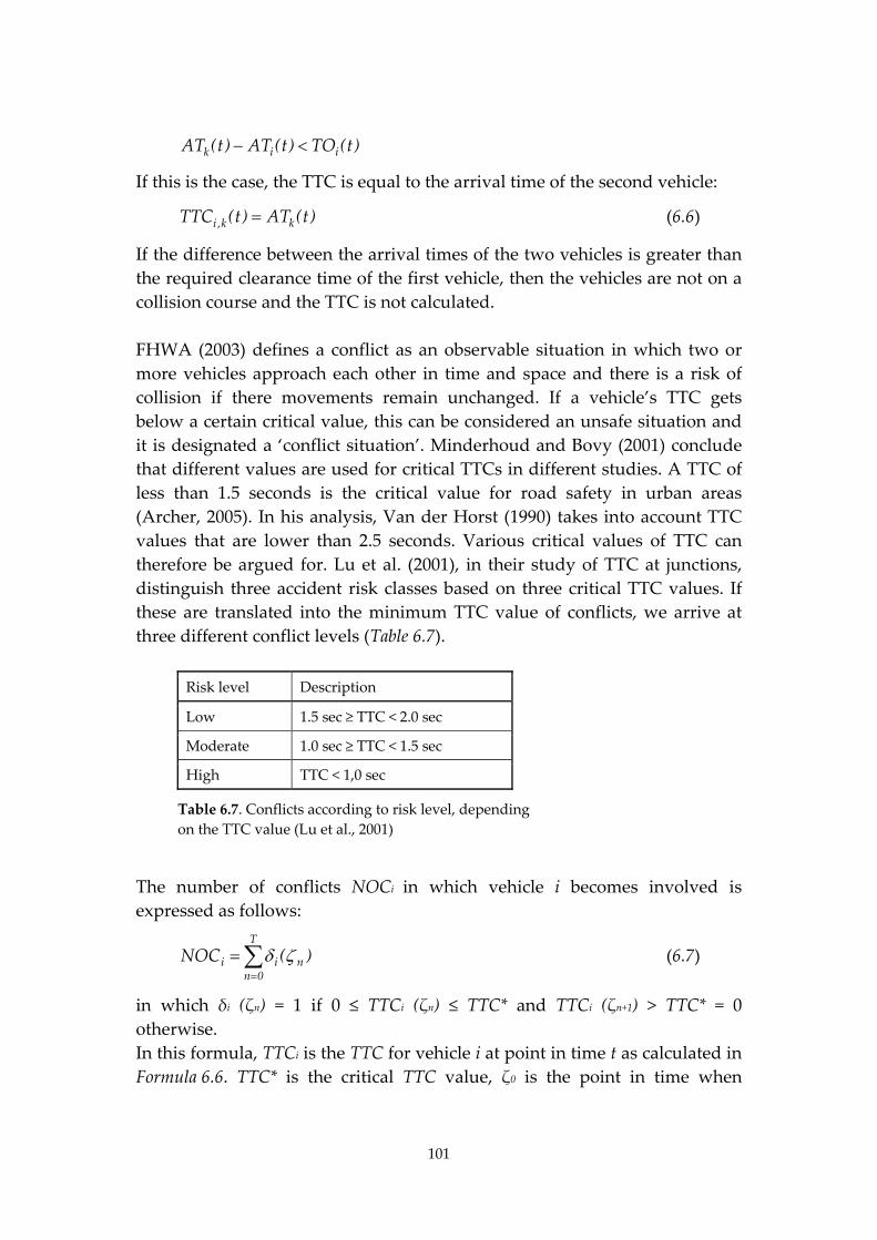
101
)t(TO)t(AT)t(AT iik
If this is the case, the TTC is equal to the arrival time of the second vehicle:
)t(AT)t(TTC kk,i (6.6)
If the difference between the arrival times of the two vehicles is greater than
the required clearance time of the first vehicle, then the vehicles are not on a
collision course and the TTC is not calculated.
FHWA (2003) defines a conflict as an observable situation in which two or
more vehicles approach each other in time and space and there is a risk of
collision if there movements remain unchanged. If a vehicle’s TTC gets
below a certain critical value, this can be considered an unsafe situation and
it is designated a ‘conflict situation’. Minderhoud and Bovy (2001) conclude
that different values are used for critical TTCs in different studies. A TTC of
less than 1.5 seconds is the critical value for road safety in urban areas
(Archer, 2005). In his analysis, Van der Horst (1990) takes into account TTC
values that are lower than 2.5 seconds. Various critical values of TTC can
therefore be argued for. Lu et al. (2001), in their study of TTC at junctions,
distinguish three accident risk classes based on three critical TTC values. If
these are translated into the minimum TTC value of conflicts, we arrive at
three different conflict levels (Table 6.7).
Risk level Description
Low 1.5 sec ≥ TTC < 2.0 sec
Moderate 1.0 sec ≥ TTC < 1.5 sec
High TTC < 1,0 sec
Table 6.7. Conflicts according to risk level, depending
on the TTC value (Lu et al., 2001)
The number of conflicts NOCi in which vehicle i becomes involved is
expressed as follows:
T
0nnii )(NOC (6.7)
in which δi (ζn) = 1 if 0 ≤ TTCi (ζn) ≤ TTC* and TTCi (ζn+1) > TTC* = 0
otherwise.
In this formula, TTCi is the TTC for vehicle i at point in time t as calculated in
Formula 6.6. TTC* is the critical TTC value, ζ0 is the point in time when
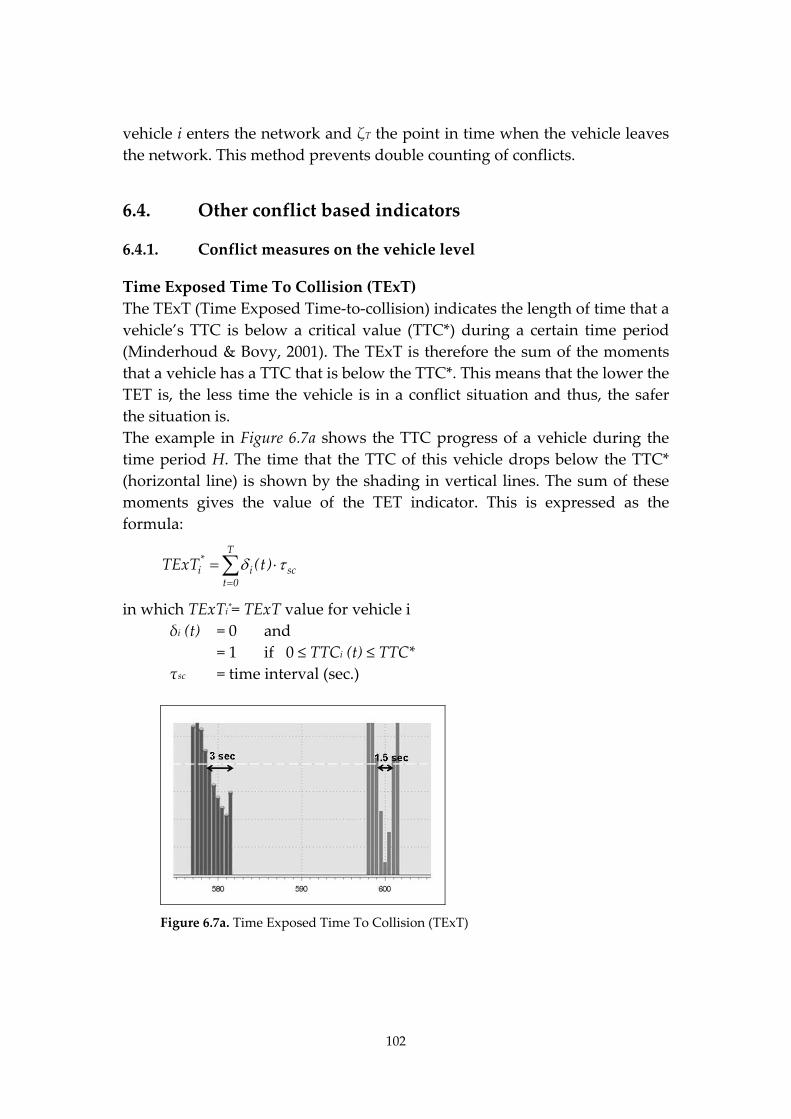
102
vehicle i enters the network and ζT the point in time when the vehicle leaves
the network. This method prevents double counting of conflicts.
6.4. Other conflict based indicators
6.4.1. Conflict measures on the vehicle level
Time Exposed Time To Collision (TExT)
The TExT (Time Exposed Time‐to‐collision) indicates the length of time that a
vehicle’s TTC is below a critical value (TTC*) during a certain time period
(Minderhoud & Bovy, 2001). The TExT is therefore the sum of the moments
that a vehicle has a TTC that is below the TTC*. This means that the lower the
TET is, the less time the vehicle is in a conflict situation and thus, the safer
the situation is.
The example in Figure 6.7a shows the TTC progress of a vehicle during the
time period H. The time that the TTC of this vehicle drops below the TTC*
(horizontal line) is shown by the shading in vertical lines. The sum of these
moments gives the value of the TET indicator. This is expressed as the
formula:
T
0tsci
*i )t(TExT
in which TExTi*= TExT value for vehicle i
δi (t) = 0 and
= 1 if 0 ≤ TTCi (t) ≤ TTC*
τsc = time interval (sec.)
Figure 6.7a. Time Exposed Time To Collision (TExT)
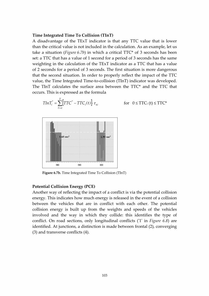
103
Time Integrated Time To Collision (TInT)
A disadvantage of the TExT indicator is that any TTC value that is lower
than the critical value is not included in the calculation. As an example, let us
take a situation (Figure 6.7b) in which a critical TTC* of 3 seconds has been
set: a TTC that has a value of 1 second for a period of 3 seconds has the same
weighting in the calculation of the TExT indicator as a TTC that has a value
of 2 seconds for a period of 3 seconds. The first situation is more dangerous
that the second situation. In order to properly reflect the impact of the TTC
value, the Time Integrated Time‐to‐collision (TInT) indicator was developed.
The TInT calculates the surface area between the TTC* and the TTC that
occurs. This is expressed as the formula
T
otsci
**i )t(TTCTTCTInT for 0 ≤ TTCi (t) ≤ TTC*
Figure 6.7b. Time Integrated Time To Collision (TInT)
Potential Collision Energy (PCE)
Another way of reflecting the impact of a conflict is via the potential collision
energy. This indicates how much energy is released in the event of a collision
between the vehicles that are in conflict with each other. The potential
collision energy is built up from the weights and speeds of the vehicles
involved and the way in which they collide: this identifies the type of
conflict. On road sections, only longitudinal conflicts (ʹ1ʹ in Figure 6.8) are
identified. At junctions, a distinction is made between frontal (2), converging
(3) and transverse conflicts (4).
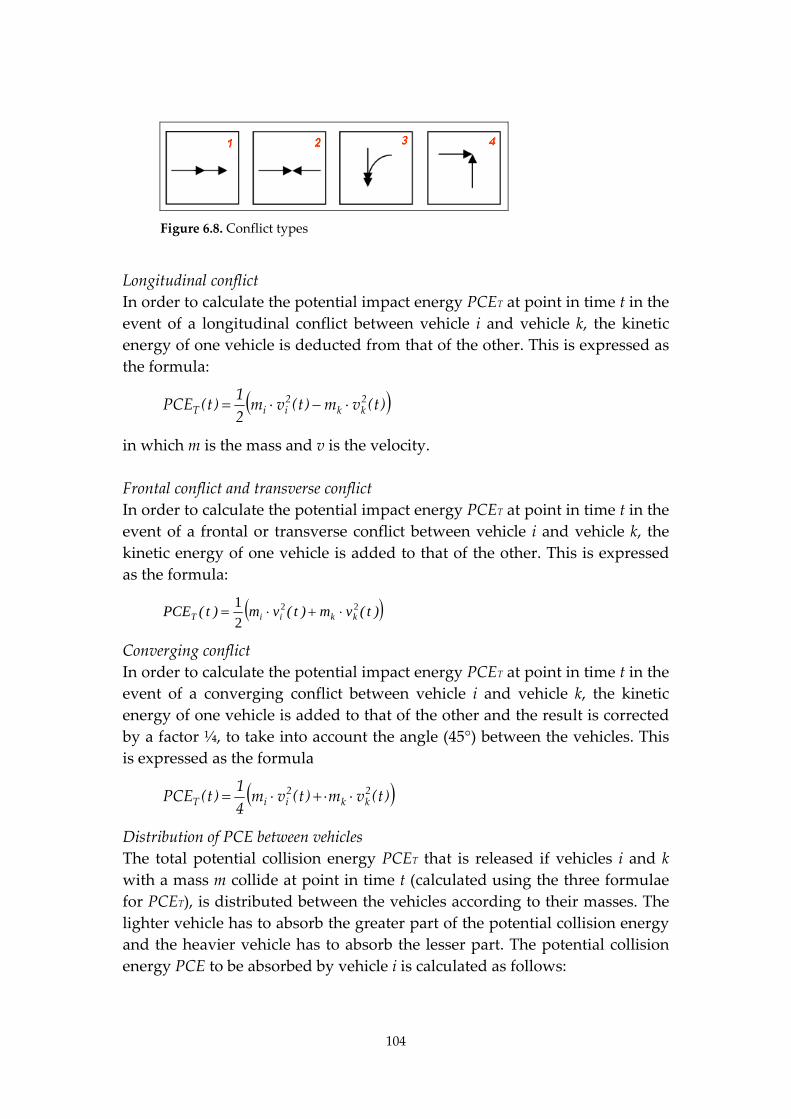
104
Figure 6.8. Conflict types
Longitudinal conflict
In order to calculate the potential impact energy PCET at point in time t in the
event of a longitudinal conflict between vehicle i and vehicle k, the kinetic
energy of one vehicle is deducted from that of the other. This is expressed as
the formula:
)t(vm)t(vm2
1)t(PCE 2
kk2iiT
in which m is the mass and v is the velocity.
Frontal conflict and transverse conflict
In order to calculate the potential impact energy PCET at point in time t in the
event of a frontal or transverse conflict between vehicle i and vehicle k, the
kinetic energy of one vehicle is added to that of the other. This is expressed
as the formula:
)t(vm)t(vm)t(PCE kkiiT22
2
1
Converging conflict
In order to calculate the potential impact energy PCET at point in time t in the
event of a converging conflict between vehicle i and vehicle k, the kinetic
energy of one vehicle is added to that of the other and the result is corrected
by a factor ¼, to take into account the angle (45°) between the vehicles. This
is expressed as the formula
)t(vm)t(vm4
1)t(PCE 2
kk2iiT
Distribution of PCE between vehicles
The total potential collision energy PCET that is released if vehicles i and k
with a mass m collide at point in time t (calculated using the three formulae
for PCET), is distributed between the vehicles according to their masses. The
lighter vehicle has to absorb the greater part of the potential collision energy
and the heavier vehicle has to absorb the lesser part. The potential collision
energy PCE to be absorbed by vehicle i is calculated as follows:
105
)t(PCE*mm
m)t(PCE T
ki
ki
.
Subsequently for vehicle k as:
)t(PCE*mm
m)t(PCE T
ki
ik
.
6.4.2. Conflict measures on higher levels
The scores of the various road safety indicators at vehicle level can be
totalled for each road section or junction to produce an indication of the
safety of a road section or junction. For example, the number of conflicts that
occur on a road section during a certain period of time is a measure of the
safety of that road section. If the absolute score is divided by an exposure
index such as the number of vehicles passing per time unit, a relative
measure is obtained. This makes it possible to compare a variety of road
sections and various simulations.
In the following sections, the safety of road sections and junctions is defined
in general terms. This implies that road safety can be assessed using a variety
of indicators at vehicle level: the number of conflicts, the TET, the TIT and
the potential collision energy. The method of arriving at road
section/junction level is the same for all four road safety indicators.
Absolute measure on road sections
The unsafety VOV on road section m during time period T is equal to the sum
of unsafety on the road, on which the number of vehicles l that pass through
road section m during time period T are involved. This is expressed as the
formula
I
iTmiTm VOVVOV
0,,,
In this the unsafety VOV is determined by the number of conflicts (NOC),
TExT, TInT, and PCE.
Relative measure on road sections
The relative unsafety RVOV for road section m (length Lm) during time period
T is equal to the absolute unsafety (as calculated using the previous formula)
divided by the product of length Lm and the number of vehicles l that pass
through road section m during time period T. This is expressed as the
formula:
106
mT,m
T,mT,m LI
VOVRVOV
Absolute measure on intersections
Longitudinal conflicts
The unsafety VOV for longitudinal conflicts at junction n for manoeuvre m
during time period T is equal to the total of the unsafety in which the I
number of vehicles executing manoeuvre m at junction n during time period
T are involved. This is expressed as the formula
I
0iT,m,n,iT,m,n VOVVOV
in which manoeuvre m can be a right turn, a left turn, going straight ahead or
a manoeuvre specified in more detail at direction level. At a 4‐arm junction,
12 directions (4 arms times 3 directions) are involved; at a 3‐arm junction, 6
directions (3 arms times 2 directions) are involved.
Converging, transverse and frontal conflicts
The relative unsafety RVOV for converging, transverse and frontal conflicts
at junction n and manoeuvre m during the period T is equal to the total
number of conflicts in which the I number of vehicles executing manoeuvre
m at junction n during time period T are involved. Because a conflict between
two vehicles takes place at the same junction and therefore counts as a
conflict for both vehicles, the conflicts for the junction must be divided by 2.
This is expressed as the formula
5.0VOVVOVI
0iT,m,n,iT,m,n
in which manoeuvre m can be a right turn, a left turn or going straight ahead.
Relative measure on intersections
The relative unsafety RVOV for junction n during time period T is equal to
the unsafety VOV, as calculated using one of the two previous formulae (for
longitudinal or other conflicts), divided by the number of passing vehicles l
executing manoeuvre m at junction n during time period T. This is expressed
as the formula
T,m,n
T,m,nT,m,n
I
VOVRVOV
107
6.4.3. Conflict measures on route level
A route r is defined as a chain of a number M of road sections and a number
N of junctions that can be followed to reach destination j from origin i. To
indicate the safety of a route, we use the relative unsafety of road sections
and junctions. The general formula is given below.
The safety of a route r between origin i and destination j (length Lr) is equal
to the sum of the unsafety VOV during time period T on the number M of
road sections and the number N of junctions, specified according to the type
of manoeuvre, that form part of the route. This is expressed as the formula:
N
0nT.m.n
M
0mT,mT,rij
VOVVOVVOV
The relative measure is formulated as:
rT,ij
T,rijT,rij LI
VOVRVOV
If a route is not taken by any vehicle, the RVOV can nevertheless be
calculated. That is because other vehicles, following different routes, will be
using the road sections of the route in question. Those vehicles will be part of
the calculation of RVOV.
From route level to OD level
Using the road safety indicators as described at the route level, it is possible
to calculate the road safety of an OD pair for all the routes that are associated
with that OD pair. Then, by making clear how vehicles are spread over these
routes, we can see to what extent vehicles select the safest route and how
many do so. Here, it is also important to include the safety level of routes
that are not selected (in this step). After all, traffic may well follow these
routes in a subsequent step. This produces a picture of the road safety of an
OD pair. We then explain, step by step, how these calculations were arrived
at.
Distribution of vehicles over all routes
The distribution of vehicles over the routes per OD pair is indicated by
calculating the percentage of the total number of vehicles per OD pair that
travel via route r. This is expressed in the formula
%100I
IV
OD
rr,OD
108
in which VOD,r is the percentage of vehicles that travel via route r from origin
H to destination B , Ir is the absolute number of vehicles that travel via route r
and IOD is the total number of vehicles that travel from origin H to
destination B.
Safety at the OD level
In order to define the safety level of an OD pair, the scores for the number of
conflicts, TExT, TInT and potential collision energy are standardised. The
standardised road safety score of a route r can be defined as follows:
%100}VV{min}VV{max
}VV{minVVVV
rrrr
rrrrs
(6.8)
in which the road safety score of a route VVr is given by the number of
conflicts (NOC), TExT, TInT and PCE.
The safety score of an OD pair is then defined as follows:
R
1r
r,ODrsOD
100
VVVVV (6.9)
in which the standardised road safety score of a route VVrs is given by NOC,
TExT, TInT and PCE.
109
7. Quantitative relationships between calculated
conflicts and recorded crashes
The best‐known safety indicator in micro‐simulation models is the ‘conflict’
situation ‐ a situation in which two vehicles approach each other and where,
if no action were taken, a crash would occur. These conflict situations in the
simulation model can be detected. This method does not necessarily relate
directly to any actual observed conflicts, let alone recorded crashes. This
chapter examines the quantitative relationship between the detected conflicts
at intersections in the model and the recorded crashes at the same locations
in reality. The methods chosen for detecting conflicts and for selecting
crashes are explained. A micro‐simulation model was constructed for a
regional road network. A description of this regional network is given as
well as the choices that were made in order to model this network.
Subsequently, the conflicts in the simulated network were detected, and the
recorded crashes were selected. Finally, both safety indicators were related to
each other.
7.1. Descriptions of the study area and the micro‐
simulation model
7.1.1. Study area
The study area is situated in the west of the Netherlands and it covers an
area of about 300 km2. The total number of inhabitants amounts to 900,000
(CBS Statline, 2008); the population density is 3,000 residents per square
kilometre. Most of the population is concentrated on the outskirts of the area.
The area contains (calculated according to Dutch proportions) one large town
(475,000 inhabitants), two medium‐sized towns (64,000 and 118,000
inhabitants), and thirteen smaller communities (4,000 to 32,000 inhabitants).
The area is traversed by two main roads (A4 and A44/N44) which are part of
the national main road network (see Figure 7.1). There are a few regional
roads that run parallel to these two main roads.
The area has many interactions with the other parts of The Netherlands and
is situated at the North Sea coast. That is why many external relationships
are oriented southwest to northeast and vice versa. The A4 motorway
connects Amsterdam with The Hague while the A44/N44 road is the
connection between Leiden, Wassenaar and The Hague. The three main
110
regional routes are the N447 road from Voorschoten to Leidschendam, the
(first part of the) N206/local roads from Katwijk to Wassenaar, and (the final
part of the) N206/local roads from Leiden, through Stompwijk to
Leidschendam (see Figure 7.1).
Car drivers do not prefer the route through Stompwijk (Goldenbeld et al.,
2006). Most of the drivers choose (one of) the other four routes. However,
Goldenbeld et al. reported that some drivers prefer the secondary road
situated next to the A44.
Three routes are situated perpendicular to the five parallel routes: a part of
the N206 road near Leiden, the N441/N448 road through Wassenaar and
Voorschoten, and the N14 road through Voorburg. Compared to the five
parallel routes, these three routes do not have many similarities, because
they connect quite different origins and destinations.
Figure 7.1. Study area
N449
N206
N206
N448
N447
N14
N44
N206
A44
N441
N206
A44
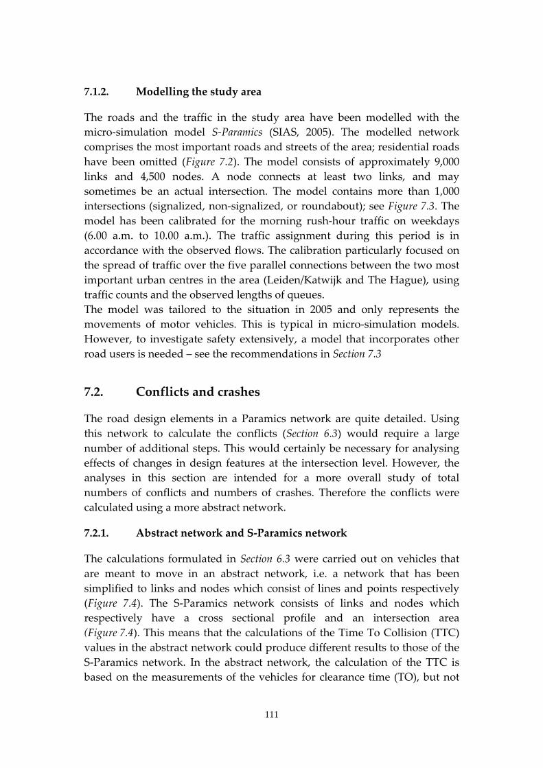
111
7.1.2. Modelling the study area
The roads and the traffic in the study area have been modelled with the
micro‐simulation model S‐Paramics (SIAS, 2005). The modelled network
comprises the most important roads and streets of the area; residential roads
have been omitted (Figure 7.2). The model consists of approximately 9,000
links and 4,500 nodes. A node connects at least two links, and may
sometimes be an actual intersection. The model contains more than 1,000
intersections (signalized, non‐signalized, or roundabout); see Figure 7.3. The
model has been calibrated for the morning rush‐hour traffic on weekdays
(6.00 a.m. to 10.00 a.m.). The traffic assignment during this period is in
accordance with the observed flows. The calibration particularly focused on
the spread of traffic over the five parallel connections between the two most
important urban centres in the area (Leiden/Katwijk and The Hague), using
traffic counts and the observed lengths of queues.
The model was tailored to the situation in 2005 and only represents the
movements of motor vehicles. This is typical in micro‐simulation models.
However, to investigate safety extensively, a model that incorporates other
road users is needed – see the recommendations in Section 7.3
7.2. Conflicts and crashes
The road design elements in a Paramics network are quite detailed. Using
this network to calculate the conflicts (Section 6.3) would require a large
number of additional steps. This would certainly be necessary for analysing
effects of changes in design features at the intersection level. However, the
analyses in this section are intended for a more overall study of total
numbers of conflicts and numbers of crashes. Therefore the conflicts were
calculated using a more abstract network.
7.2.1. Abstract network and S‐Paramics network
The calculations formulated in Section 6.3 were carried out on vehicles that
are meant to move in an abstract network, i.e. a network that has been
simplified to links and nodes which consist of lines and points respectively
(Figure 7.4). The S‐Paramics network consists of links and nodes which
respectively have a cross sectional profile and an intersection area
(Figure 7.4). This means that the calculations of the Time To Collision (TTC)
values in the abstract network could produce different results to those of the
S‐Paramics network. In the abstract network, the calculation of the TTC is
based on the measurements of the vehicles for clearance time (TO), but not
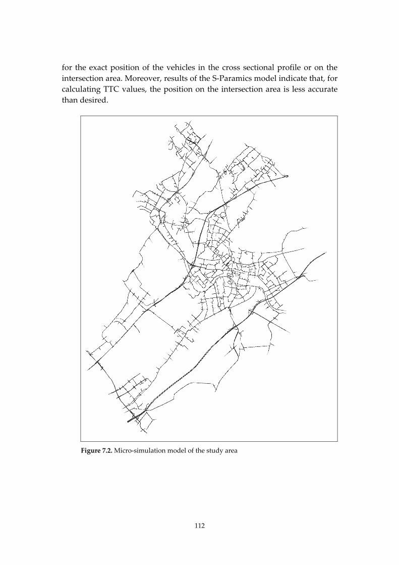
112
for the exact position of the vehicles in the cross sectional profile or on the
intersection area. Moreover, results of the S‐Paramics model indicate that, for
calculating TTC values, the position on the intersection area is less accurate
than desired.
Figure 7.2. Micro‐simulation model of the study area
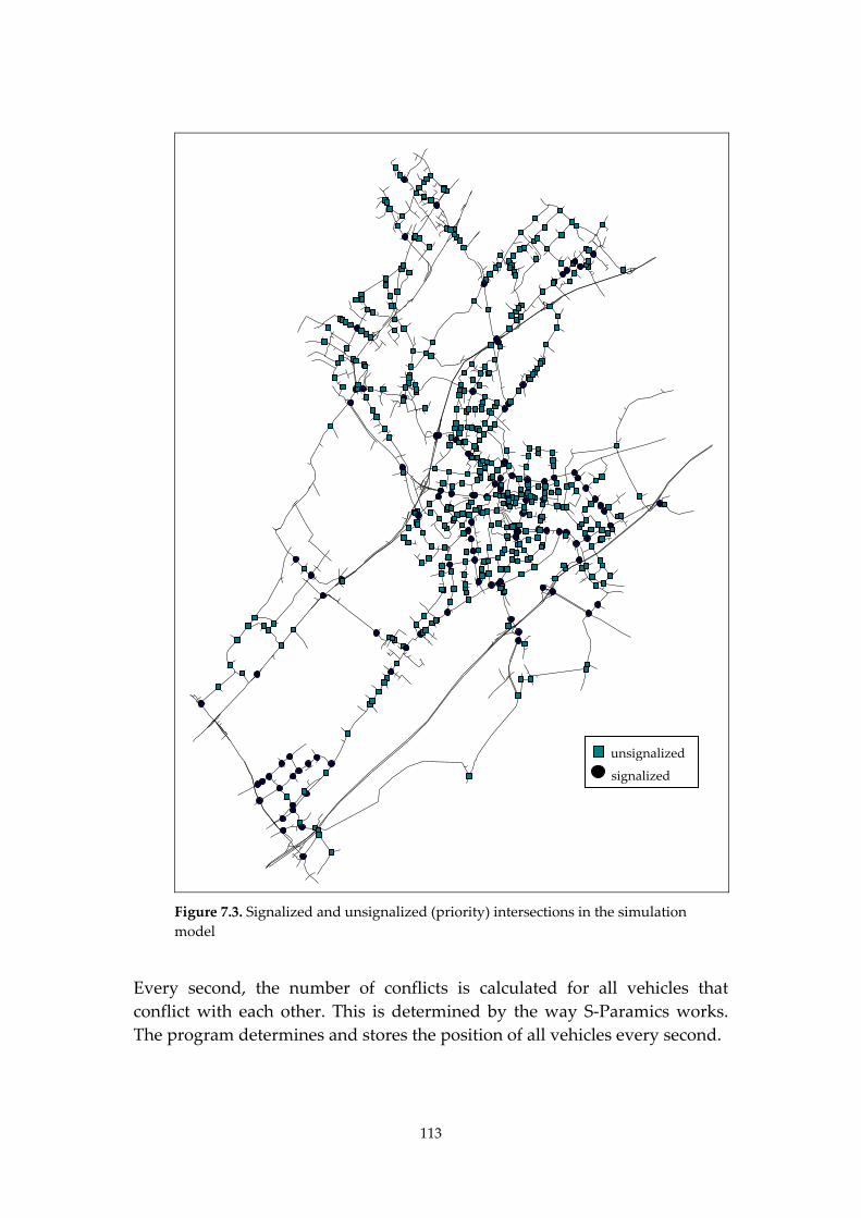
113
Figure 7.3. Signalized and unsignalized (priority) intersections in the simulation
model
Every second, the number of conflicts is calculated for all vehicles that
conflict with each other. This is determined by the way S‐Paramics works.
The program determines and stores the position of all vehicles every second.
signalized
unsignalized
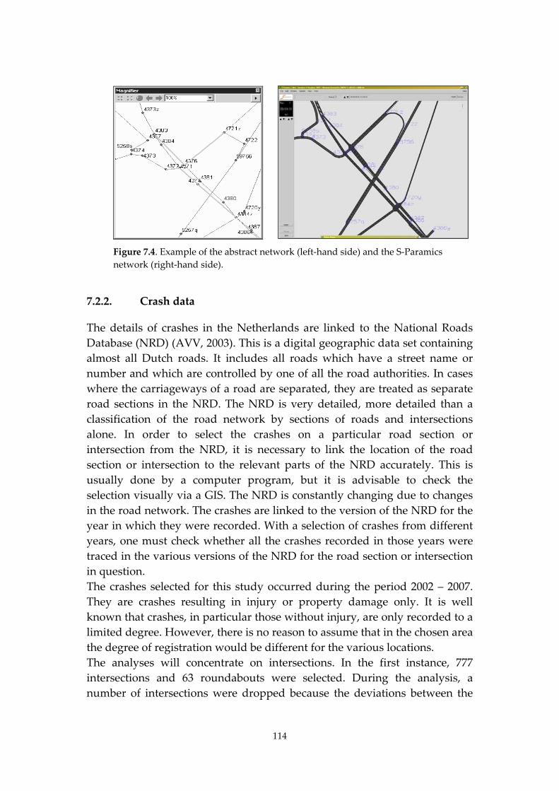
114
Figure 7.4. Example of the abstract network (left‐hand side) and the S‐Paramics
network (right‐hand side).
7.2.2. Crash data
The details of crashes in the Netherlands are linked to the National Roads
Database (NRD) (AVV, 2003). This is a digital geographic data set containing
almost all Dutch roads. It includes all roads which have a street name or
number and which are controlled by one of all the road authorities. In cases
where the carriageways of a road are separated, they are treated as separate
road sections in the NRD. The NRD is very detailed, more detailed than a
classification of the road network by sections of roads and intersections
alone. In order to select the crashes on a particular road section or
intersection from the NRD, it is necessary to link the location of the road
section or intersection to the relevant parts of the NRD accurately. This is
usually done by a computer program, but it is advisable to check the
selection visually via a GIS. The NRD is constantly changing due to changes
in the road network. The crashes are linked to the version of the NRD for the
year in which they were recorded. With a selection of crashes from different
years, one must check whether all the crashes recorded in those years were
traced in the various versions of the NRD for the road section or intersection
in question.
The crashes selected for this study occurred during the period 2002 – 2007.
They are crashes resulting in injury or property damage only. It is well
known that crashes, in particular those without injury, are only recorded to a
limited degree. However, there is no reason to assume that in the chosen area
the degree of registration would be different for the various locations.
The analyses will concentrate on intersections. In the first instance, 777
intersections and 63 roundabouts were selected. During the analysis, a
number of intersections were dropped because the deviations between the
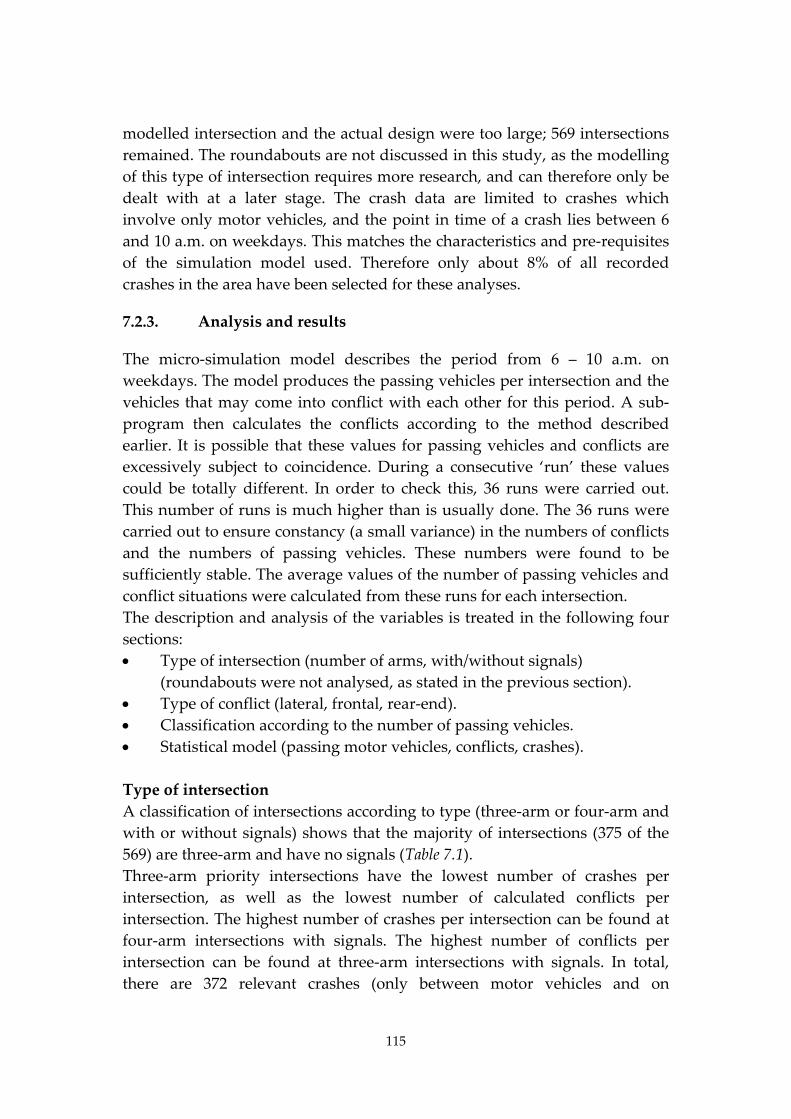
115
modelled intersection and the actual design were too large; 569 intersections
remained. The roundabouts are not discussed in this study, as the modelling
of this type of intersection requires more research, and can therefore only be
dealt with at a later stage. The crash data are limited to crashes which
involve only motor vehicles, and the point in time of a crash lies between 6
and 10 a.m. on weekdays. This matches the characteristics and pre‐requisites
of the simulation model used. Therefore only about 8% of all recorded
crashes in the area have been selected for these analyses.
7.2.3. Analysis and results
The micro‐simulation model describes the period from 6 – 10 a.m. on
weekdays. The model produces the passing vehicles per intersection and the
vehicles that may come into conflict with each other for this period. A sub‐
program then calculates the conflicts according to the method described
earlier. It is possible that these values for passing vehicles and conflicts are
excessively subject to coincidence. During a consecutive ‘run’ these values
could be totally different. In order to check this, 36 runs were carried out.
This number of runs is much higher than is usually done. The 36 runs were
carried out to ensure constancy (a small variance) in the numbers of conflicts
and the numbers of passing vehicles. These numbers were found to be
sufficiently stable. The average values of the number of passing vehicles and
conflict situations were calculated from these runs for each intersection.
The description and analysis of the variables is treated in the following four
sections:
Type of intersection (number of arms, with/without signals)
(roundabouts were not analysed, as stated in the previous section).
Type of conflict (lateral, frontal, rear‐end).
Classification according to the number of passing vehicles.
Statistical model (passing motor vehicles, conflicts, crashes).
Type of intersection
A classification of intersections according to type (three‐arm or four‐arm and
with or without signals) shows that the majority of intersections (375 of the
569) are three‐arm and have no signals (Table 7.1).
Three‐arm priority intersections have the lowest number of crashes per
intersection, as well as the lowest number of calculated conflicts per
intersection. The highest number of crashes per intersection can be found at
four‐arm intersections with signals. The highest number of conflicts per
intersection can be found at three‐arm intersections with signals. In total,
there are 372 relevant crashes (only between motor vehicles and on
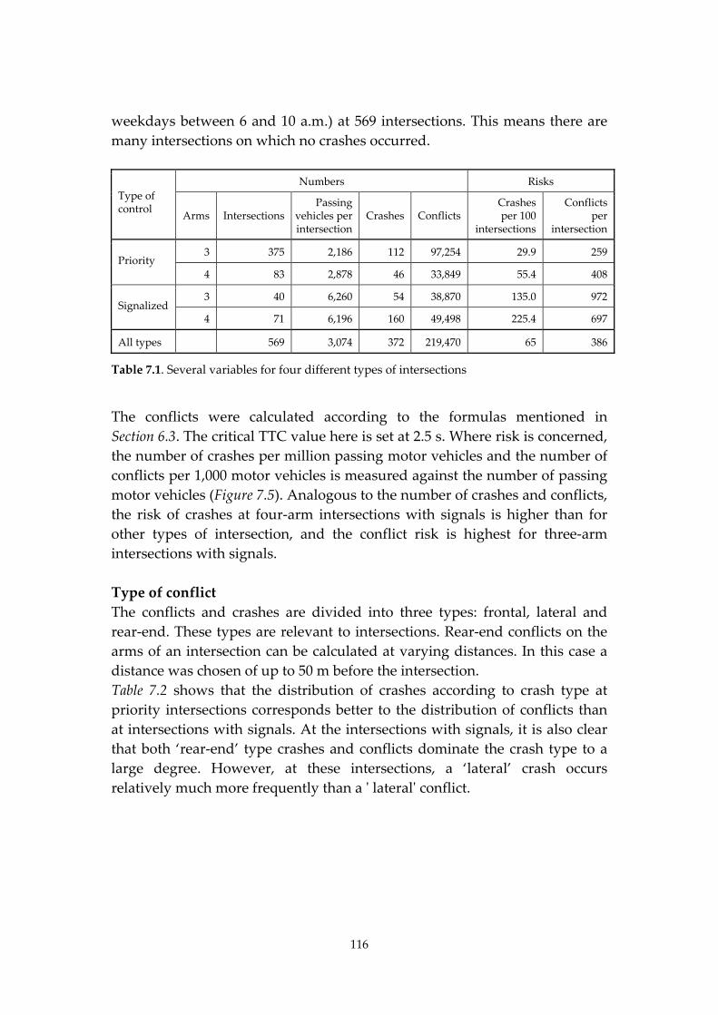
116
weekdays between 6 and 10 a.m.) at 569 intersections. This means there are
many intersections on which no crashes occurred.
Numbers Risks
Type of control
Arms Intersections Passing
vehicles per intersection
Crashes Conflicts Crashes per 100
intersections
Conflicts per
intersection
3 375 2,186 112 97,254 29.9 259 Priority
4 83 2,878 46 33,849 55.4 408
3 40 6,260 54 38,870 135.0 972 Signalized
4 71 6,196 160 49,498 225.4 697
All types 569 3,074 372 219,470 65 386
Table 7.1. Several variables for four different types of intersections
The conflicts were calculated according to the formulas mentioned in
Section 6.3. The critical TTC value here is set at 2.5 s. Where risk is concerned,
the number of crashes per million passing motor vehicles and the number of
conflicts per 1,000 motor vehicles is measured against the number of passing
motor vehicles (Figure 7.5). Analogous to the number of crashes and conflicts,
the risk of crashes at four‐arm intersections with signals is higher than for
other types of intersection, and the conflict risk is highest for three‐arm
intersections with signals.
Type of conflict
The conflicts and crashes are divided into three types: frontal, lateral and
rear‐end. These types are relevant to intersections. Rear‐end conflicts on the
arms of an intersection can be calculated at varying distances. In this case a
distance was chosen of up to 50 m before the intersection.
Table 7.2 shows that the distribution of crashes according to crash type at
priority intersections corresponds better to the distribution of conflicts than
at intersections with signals. At the intersections with signals, it is also clear
that both ‘rear‐end’ type crashes and conflicts dominate the crash type to a
large degree. However, at these intersections, a ‘lateral’ crash occurs
relatively much more frequently than a ʹ lateralʹ conflict.
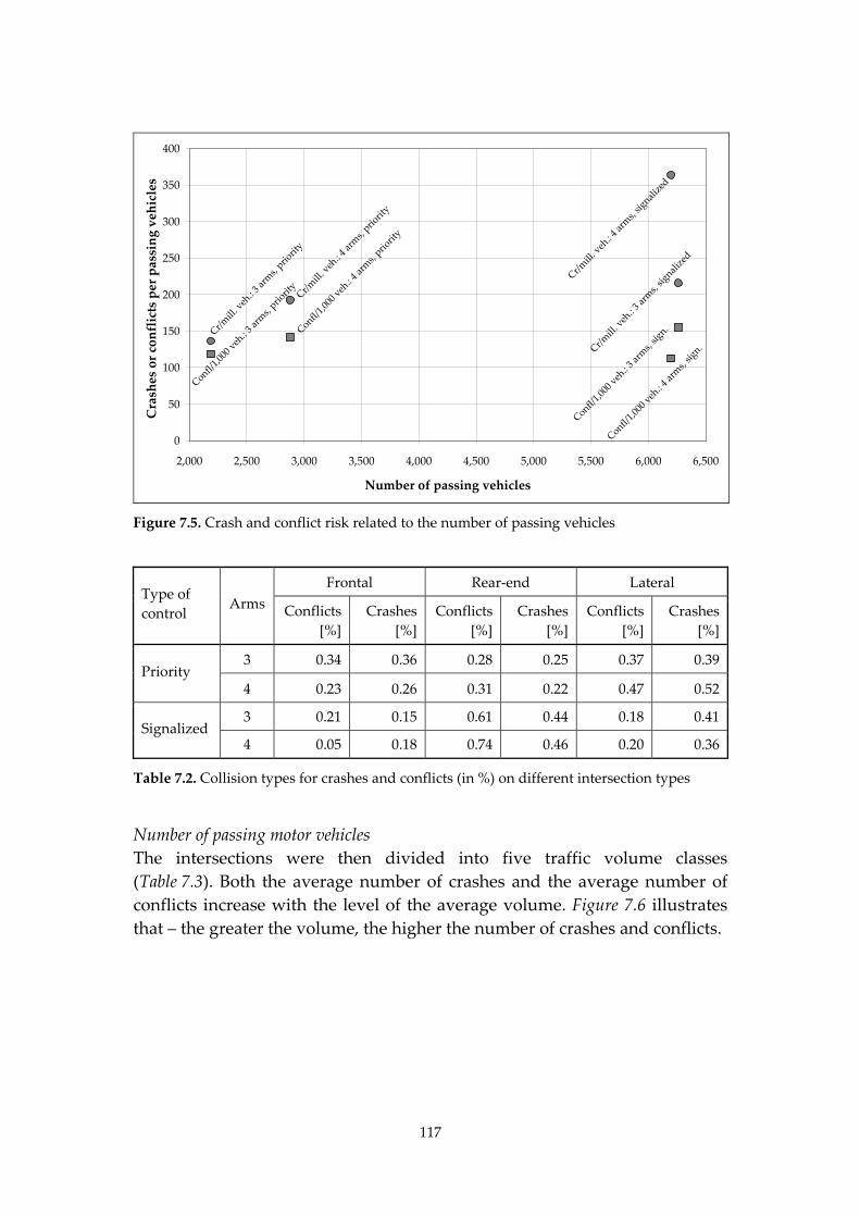
117
Cr/mill. veh.: 3 arms, priority
Cr/mill. veh.: 4 arms, priority
Cr/mill. veh.: 3 arms, signalized
Cr/mill. veh.: 4 arms, signalized
Confl/1,000 veh.: 3 arms, priority
Confl/1,000 veh.: 4 arms, priority
Confl/1,000 veh.: 3 arms, sign.
Confl/1,000 veh.: 4 arms, sign.
0
50
100
150
200
250
300
350
400
2,000 2,500 3,000 3,500 4,000 4,500 5,000 5,500 6,000 6,500
Number of passing vehicles
Crashes or conflicts per passing vehicles
Figure 7.5. Crash and conflict risk related to the number of passing vehicles
Frontal Rear‐end Lateral Type of
control Arms
Conflicts
[%]
Crashes
[%]
Conflicts
[%]
Crashes
[%]
Conflicts
[%]
Crashes
[%]
3 0.34 0.36 0.28 0.25 0.37 0.39 Priority
4 0.23 0.26 0.31 0.22 0.47 0.52
3 0.21 0.15 0.61 0.44 0.18 0.41 Signalized
4 0.05 0.18 0.74 0.46 0.20 0.36
Table 7.2. Collision types for crashes and conflicts (in %) on different intersection types
Number of passing motor vehicles
The intersections were then divided into five traffic volume classes
(Table 7.3). Both the average number of crashes and the average number of
conflicts increase with the level of the average volume. Figure 7.6 illustrates
that – the greater the volume, the higher the number of crashes and conflicts.
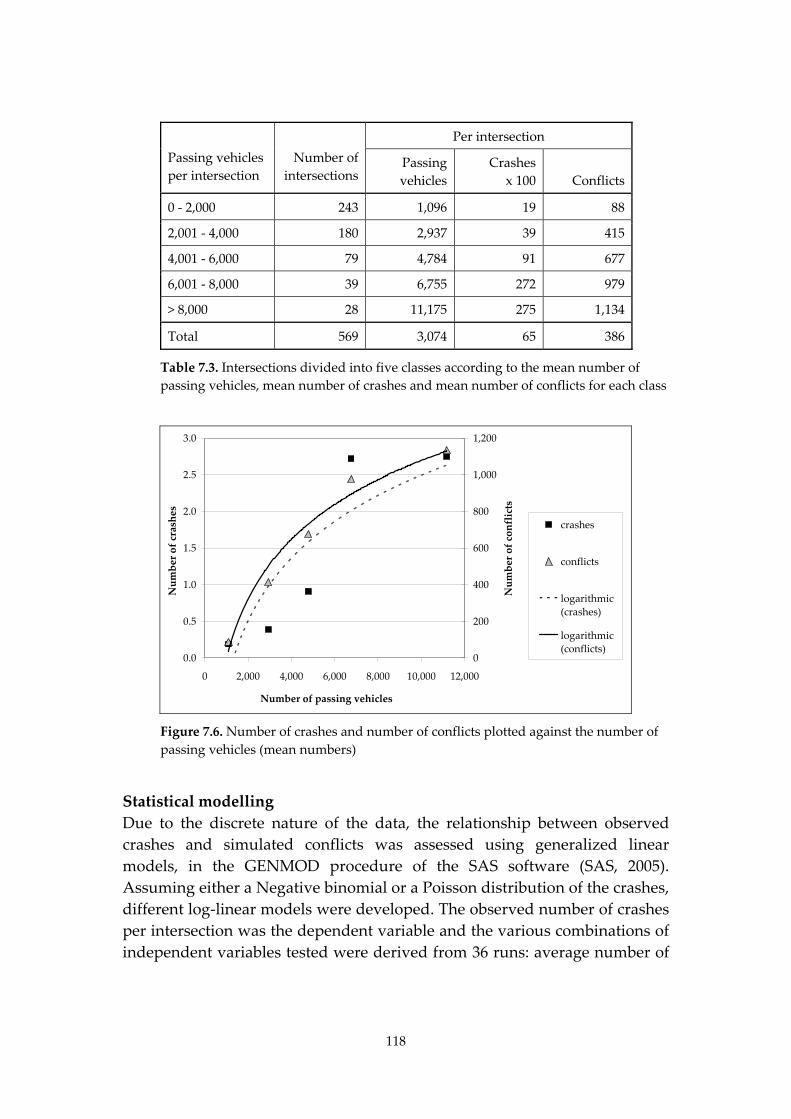
118
Per intersection
Passing vehicles
per intersection
Number of
intersections Passing
vehicles
Crashes
x 100 Conflicts
0 ‐ 2,000 243 1,096 19 88
2,001 ‐ 4,000 180 2,937 39 415
4,001 ‐ 6,000 79 4,784 91 677
6,001 ‐ 8,000 39 6,755 272 979
> 8,000 28 11,175 275 1,134
Total 569 3,074 65 386
Table 7.3. Intersections divided into five classes according to the mean number of
passing vehicles, mean number of crashes and mean number of conflicts for each class
0.0
0.5
1.0
1.5
2.0
2.5
3.0
0 2,000 4,000 6,000 8,000 10,000 12,000
Number of passing vehicles
Number of crashes
0
200
400
600
800
1,000
1,200
Number of conflicts
crashes
conflicts
logarithmic
(crashes)
logarithmic
(conflicts)
Figure 7.6. Number of crashes and number of conflicts plotted against the number of
passing vehicles (mean numbers)
Statistical modelling
Due to the discrete nature of the data, the relationship between observed
crashes and simulated conflicts was assessed using generalized linear
models, in the GENMOD procedure of the SAS software (SAS, 2005).
Assuming either a Negative binomial or a Poisson distribution of the crashes,
different log‐linear models were developed. The observed number of crashes
per intersection was the dependent variable and the various combinations of
independent variables tested were derived from 36 runs: average number of
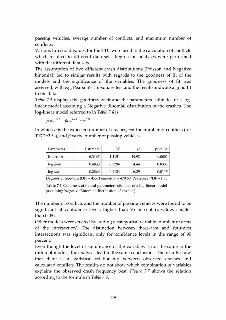
119
passing vehicles, average number of conflicts, and maximum number of
conflicts.
Various threshold values for the TTC were used in the calculation of conflicts
which resulted in different data sets. Regression analyses were performed
with the different data sets.
The assumption of two different crash distributions (Poisson and Negative
binomial) led to similar results with regards to the goodness of fit of the
models and the significance of the variables. The goodness of fit was
assessed, with e.g. Pearson’s chi‐square test and the results indicate a good fit
to the data.
Table 7.4 displays the goodness of fit and the parameters estimates of a log‐
linear model assuming a Negative Binomial distribution of the crashes. The
log‐linear model referred to in Table 7.4 is:
28.048.031.6 nocflowe
In which is the expected number of crashes, noc the number of conflicts (for
TTC*=2.5s), and flow the number of passing vehicles.
Parameter Estimate SE 2 p‐value
Intercept ‐6.3165 1.4151 19.92 <.0001
log flow 0.4838 0.2296 4.44 0.0351
log noc 0.2869 0.1134 6.39 0.0115
Degrees of freedom (DF) = 455; Pearson 2 = 470.60; Pearson 2 /DF = 1.03
Table 7.4. Goodness of fit and parameter estimates of a log‐linear model
(assuming Negative Binomial distribution of crashes)
The number of conflicts and the number of passing vehicles were found to be
significant at confidence levels higher than 95 percent (p‐values smaller
than 0.05).
Other models were created by adding a categorical variable ‘number of arms
of the intersection’. The distinction between three‐arm and four‐arm
intersections was significant only for confidence levels in the range of 90
percent.
Even though the level of significance of the variables is not the same in the
different models, the analyses lead to the same conclusions. The results show
that there is a statistical relationship between observed crashes and
calculated conflicts. The results do not show which combination of variables
explains the observed crash frequency best. Figure 7.7 shows the relation
according to the formula in Table 7.4.
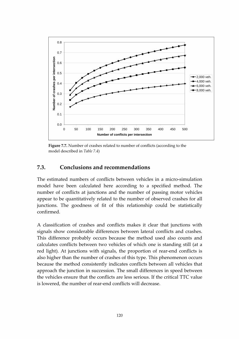
120
0.0
0.1
0.2
0.3
0.4
0.5
0.6
0.7
0.8
0 50 100 150 200 250 300 350 400 450 500
Number of conflicts per intersection
Nu
mb
er o
f cr
ash
es
per
in
ters
ecti
on
2,000 veh.4,000 veh.6,000 veh.8,000 veh.
Figure 7.7. Number of crashes related to number of conflicts (according to the
model described in Table 7.4)
7.3. Conclusions and recommendations
The estimated numbers of conflicts between vehicles in a micro‐simulation
model have been calculated here according to a specified method. The
number of conflicts at junctions and the number of passing motor vehicles
appear to be quantitatively related to the number of observed crashes for all
junctions. The goodness of fit of this relationship could be statistically
confirmed.
A classification of crashes and conflicts makes it clear that junctions with
signals show considerable differences between lateral conflicts and crashes.
This difference probably occurs because the method used also counts and
calculates conflicts between two vehicles of which one is standing still (at a
red light). At junctions with signals, the proportion of rear‐end conflicts is
also higher than the number of crashes of this type. This phenomenon occurs
because the method consistently indicates conflicts between all vehicles that
approach the junction in succession. The small differences in speed between
the vehicles ensure that the conflicts are less serious. If the critical TTC value
is lowered, the number of rear‐end conflicts will decrease.
121
The model does not allow for detecting conflicts regarding red‐light running.
So crashes of this type will not be ʹpredictedʹ by the model.
The four‐arm junctions with signals show a considerable deviation between
the number of conflicts and crashes, both per junction and per passing
vehicle (risk). It is possible that these differences and deviations are linked to
the chosen method (via the road link) for determining conflicts. A detailed
definition of the driving course through the intersection area could well
provide a different result. It is possible that there are junctions showing
deviations due to modelling errors or excessive simplification (deviations
between the model and reality).
Models like S‐Paramics are, to a great extent, black boxes. For research
purposes, the internal modelling of vehicle movements and interactions
should be clearer.
The model does not yet take traffic other than motor vehicles into account.
Addition of cyclist and pedestrian movements is, however, desired.
122
8. Quantitative relationships between route
criteria, calculated conflicts, and travel time
This chapter focuses on the design of a method enabling the planner to find
out the safety effects of existing route choice, and the effects resulting from
changes in route choice. A description of the road safety of a route can be
made by constructing a so‐called ʹroute diagramʹ. This diagram can be
checked according to a series of criteria, each representing requirements for a
route choice according to the principles of Sustainable Safety. Each criterion
of the route diagram contributes to the entire safety level of a route by the
number of ʹdemerit pointsʹ scored by the criterion. Some additional safety
criteria are added in order to find the total safety level of a route, referred to
as the ʹDV scoreʹ2). The relative importance of a criterion can be changed by
introducing coefficients of weight. Such coefficients should express the
contribution of a criterion to the safety level of the DV score.
The DV scores are applied to a regional network and are demonstrated in a
micro‐simulation model of this network.
The quantitative relationships between the different types of DV scores and
the number of simulated conflicts are analysed. This analysis focuses on the
alternative routes within each OD‐pair. The analysis is extended to a check
on the requirement in Sustainable Safety regarding the routes within an OD:
ʹthe shortest route should also be the safest routeʹ (Chapter 1).
8.1. Examples of applying DV scores to the study area
In Section 6.2, several safety scores were defined. Henceforth, the safety score
for a route VVrs (as defined in Formula 6.8) will be called DV score. The safety
score for an OD pair VVOD (using Formula 6.9) will be called OD score
hereafter. Route stars were introduced to visualize the contribution of each
safety criterion to the safety level of a route. The route stars of all routes
within an OD can be used to compare the routes regarding their safety
criteria.
The study area was described in Section 7.1. Within this area, some of the
safety indicators will be applied to show the characteristics of the method.
The regular DV score was calculated for routes within two OD pairs. These
2) DV: abbreviation of Duurzaam Veilig, which is Dutch for Sustainable Safety
123
OD pairs were selected because of the importance of the routes involved. The
questionnaire by Goldenbeld et al. (2006) also focused on these routes.
Given the DV scores, the OD score was calculated. The OD score takes into
account the actual use of each route. A route with a high DV score, carrying
most of the traffic of the OD‐pair, will contribute (positively) to the OD score
to a large extent. The OD score will be low if most of the traffic uses a route
with a low DV score. The DV score can be calculated for a route carrying no
traffic within the OD‐pair but this route will not contribute to the OD score.
8.1.1. From Origin Leiden (Southern side) to Destination
Leidschendam
Most of the journeys between Leiden (Southern side) and Leidschendam
follow the four routes shown in Figure 8.1. According to Goldenbeld et al.
(2006) the routes are used as stated below (in percentages of the total OD
traffic volume):
A4: 32%;
A44 ‐ N44: 54%;
Voorschoten ‐ N447: 10%;
Voorschoten ‐ N448 ‐ N44: 3%.
In order to simplify the calculations the beginnings and endings of all routes
are cut off. So the routes only consist of main roads (through roads and
distributor roads), while access roads are left out. The routes along the A4
and along the combination A44 ‐ N44 only consist of motorways and quasi
motorways. These routes attract most of the traffic in spite of the many
queues on these roads. The other two routes, through Voorschoten, are
characterized by a lower capacity, lower speed limits and more disruptions
by crossing traffic. Table 8.1 shows the scores Cji on the criteria. From these
scores the DV scores are calculated, see Table 8.2, row No. 1. The route stars
for these routes are shown in Figure 8.2.
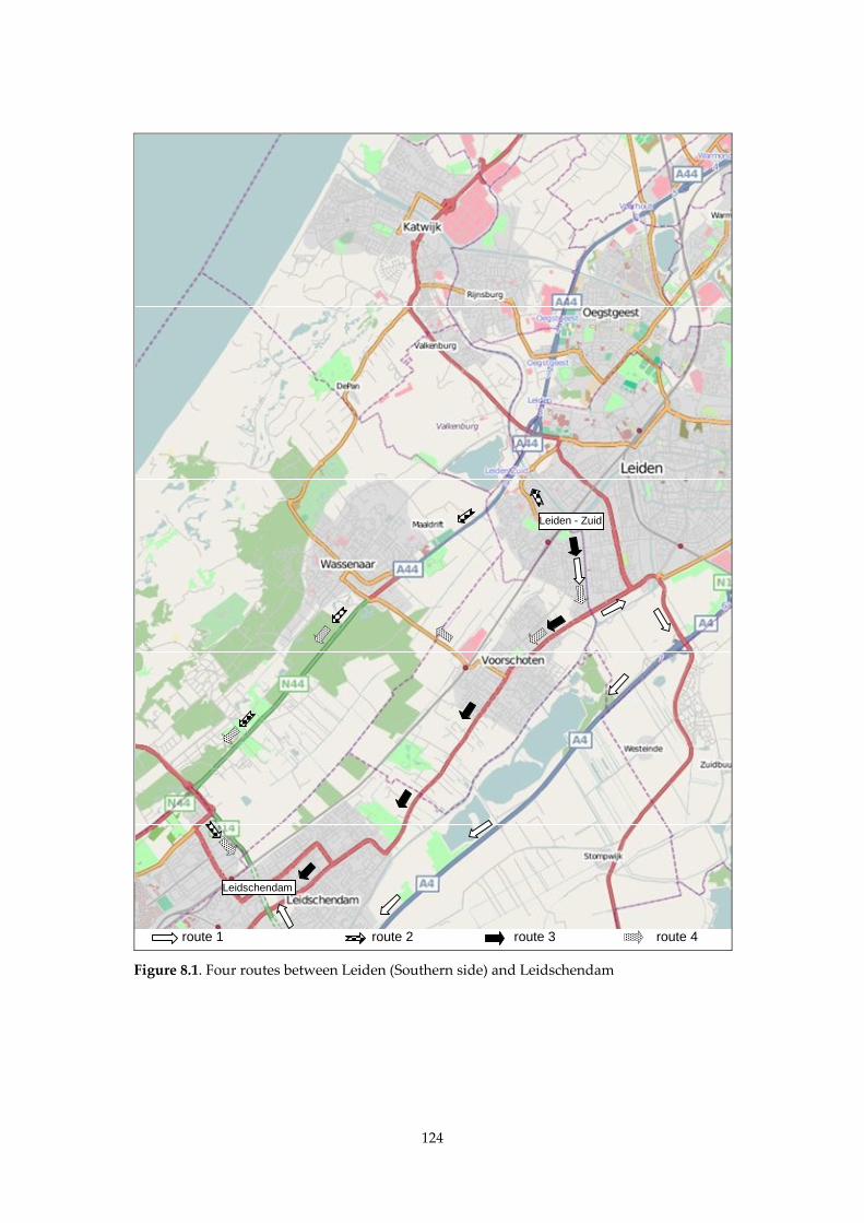
124
route 1 route 2 route 3 route 4
Leidschendam
Leiden - Zuid
Figure 8.1. Four routes between Leiden (Southern side) and Leidschendam
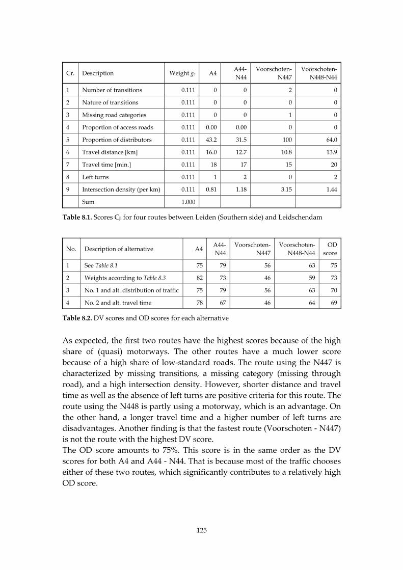
125
Cr. Description Weight gc A4 A44‐
N44
Voorschoten‐
N447
Voorschoten‐
N448‐N44
1 Number of transitions 0.111 0 0 2 0
2 Nature of transitions 0.111 0 0 0 0
3 Missing road categories 0.111 0 0 1 0
4 Proportion of access roads 0.111 0.00 0.00 0 0
5 Proportion of distributors 0.111 43.2 31.5 100 64.0
6 Travel distance [km] 0.111 16.0 12.7 10.8 13.9
7 Travel time [min.] 0.111 18 17 15 20
8 Left turns 0.111 1 2 0 2
9 Intersection density (per km) 0.111 0.81 1.18 3.15 1.44
Sum 1.000
Table 8.1. Scores Cji for four routes between Leiden (Southern side) and Leidschendam
No. Description of alternative A4 A44‐
N44
Voorschoten‐
N447
Voorschoten‐
N448‐N44
OD
score
1 See Table 8.1 75 79 56 63 75
2 Weights according to Table 8.3 82 73 46 59 73
3 No. 1 and alt. distribution of traffic 75 79 56 63 70
4 No. 2 and alt. travel time 78 67 46 64 69
Table 8.2. DV scores and OD scores for each alternative
As expected, the first two routes have the highest scores because of the high
share of (quasi) motorways. The other routes have a much lower score
because of a high share of low‐standard roads. The route using the N447 is
characterized by missing transitions, a missing category (missing through
road), and a high intersection density. However, shorter distance and travel
time as well as the absence of left turns are positive criteria for this route. The
route using the N448 is partly using a motorway, which is an advantage. On
the other hand, a longer travel time and a higher number of left turns are
disadvantages. Another finding is that the fastest route (Voorschoten ‐ N447)
is not the route with the highest DV score.
The OD score amounts to 75%. This score is in the same order as the DV
scores for both A4 and A44 ‐ N44. That is because most of the traffic chooses
either of these two routes, which significantly contributes to a relatively high
OD score.
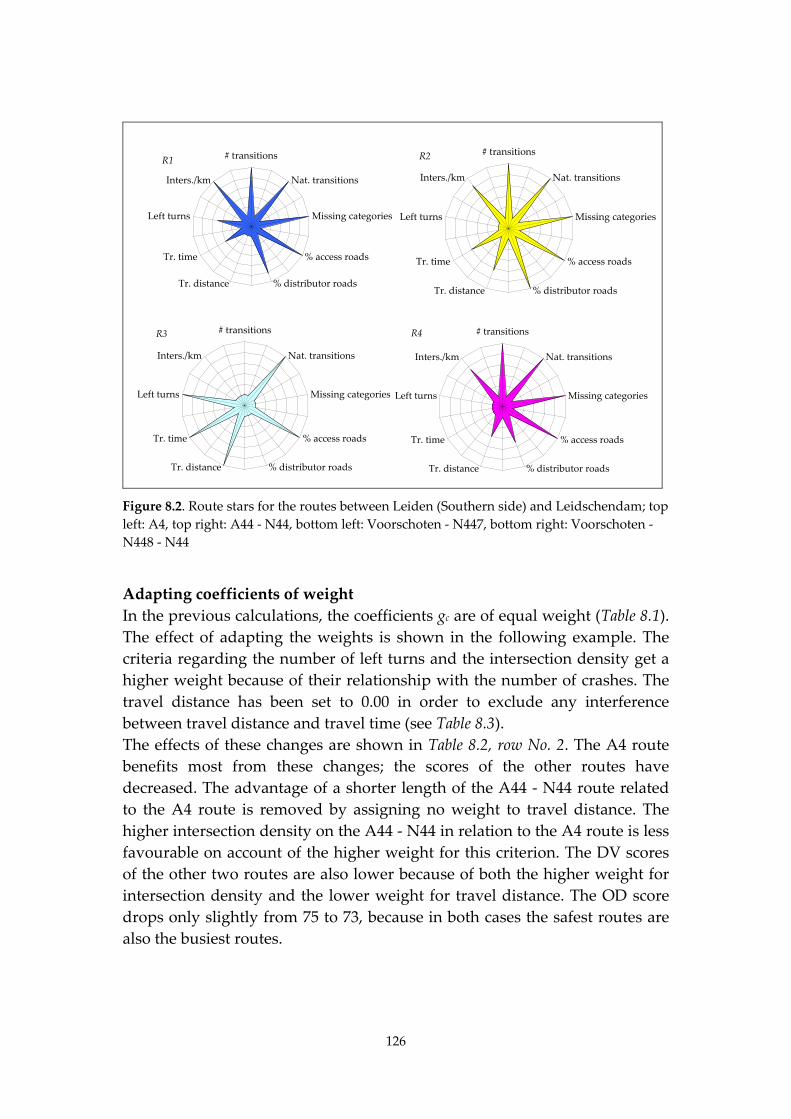
126
R2
-0.2
0
0.2
0.4
0.6
0.8
1
# transitions
Nat. transitions
Missing categories
% access roads
% distributor roadsTr. distance
Tr. time
Left turns
Inters./km
R4
-0.2
0
0.2
0.4
0.6
0.8
1
# transitions
Nat. transitions
Missing categories
% access roads
% distributor roadsTr. distance
Tr. time
Left turns
Inters./km
R1
-0.2
0
0.2
0.4
0.6
0.8
1
# transitions
Nat. transitions
Missing categories
% access roads
% distributor roadsTr. distance
Tr. time
Left turns
Inters./km
R3
-0.2
0
0.2
0.4
0.6
0.8
1
# transitions
Nat. transitions
Missing categories
% access roads
% distributor roadsTr. distance
Tr. time
Left turns
Inters./km
Figure 8.2. Route stars for the routes between Leiden (Southern side) and Leidschendam; top
left: A4, top right: A44 ‐ N44, bottom left: Voorschoten ‐ N447, bottom right: Voorschoten ‐
N448 ‐ N44
Adapting coefficients of weight
In the previous calculations, the coefficients gc are of equal weight (Table 8.1).
The effect of adapting the weights is shown in the following example. The
criteria regarding the number of left turns and the intersection density get a
higher weight because of their relationship with the number of crashes. The
travel distance has been set to 0.00 in order to exclude any interference
between travel distance and travel time (see Table 8.3).
The effects of these changes are shown in Table 8.2, row No. 2. The A4 route
benefits most from these changes; the scores of the other routes have
decreased. The advantage of a shorter length of the A44 ‐ N44 route related
to the A4 route is removed by assigning no weight to travel distance. The
higher intersection density on the A44 ‐ N44 in relation to the A4 route is less
favourable on account of the higher weight for this criterion. The DV scores
of the other two routes are also lower because of both the higher weight for
intersection density and the lower weight for travel distance. The OD score
drops only slightly from 75 to 73, because in both cases the safest routes are
also the busiest routes.
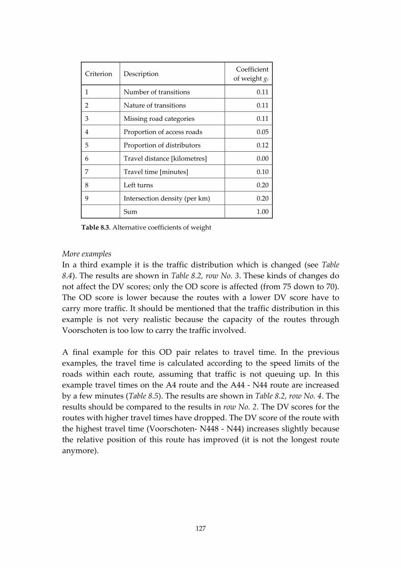
127
Criterion Description Coefficient
of weight gc
1 Number of transitions 0.11
2 Nature of transitions 0.11
3 Missing road categories 0.11
4 Proportion of access roads 0.05
5 Proportion of distributors 0.12
6 Travel distance [kilometres] 0.00
7 Travel time [minutes] 0.10
8 Left turns 0.20
9 Intersection density (per km) 0.20
Sum 1.00
Table 8.3. Alternative coefficients of weight
More examples
In a third example it is the traffic distribution which is changed (see Table
8.4). The results are shown in Table 8.2, row No. 3. These kinds of changes do
not affect the DV scores; only the OD score is affected (from 75 down to 70).
The OD score is lower because the routes with a lower DV score have to
carry more traffic. It should be mentioned that the traffic distribution in this
example is not very realistic because the capacity of the routes through
Voorschoten is too low to carry the traffic involved.
A final example for this OD pair relates to travel time. In the previous
examples, the travel time is calculated according to the speed limits of the
roads within each route, assuming that traffic is not queuing up. In this
example travel times on the A4 route and the A44 ‐ N44 route are increased
by a few minutes (Table 8.5). The results are shown in Table 8.2, row No. 4. The
results should be compared to the results in row No. 2. The DV scores for the
routes with higher travel times have dropped. The DV score of the route with
the highest travel time (Voorschoten‐ N448 ‐ N44) increases slightly because
the relative position of this route has improved (it is not the longest route
anymore).
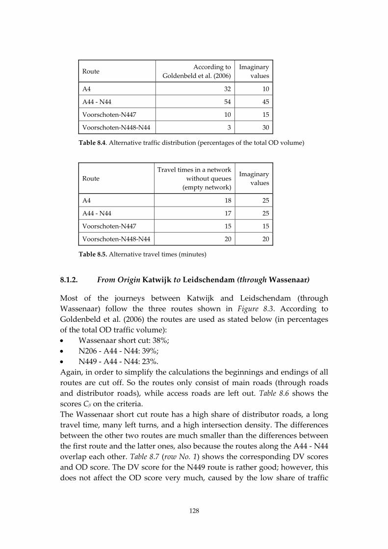
128
Route According to
Goldenbeld et al. (2006)
Imaginary
values
A4 32 10
A44 ‐ N44 54 45
Voorschoten‐N447 10 15
Voorschoten‐N448‐N44 3 30
Table 8.4. Alternative traffic distribution (percentages of the total OD volume)
Route
Travel times in a network
without queues
(empty network)
Imaginary
values
A4 18 25
A44 ‐ N44 17 25
Voorschoten‐N447 15 15
Voorschoten‐N448‐N44 20 20
Table 8.5. Alternative travel times (minutes)
8.1.2. From Origin Katwijk to Leidschendam (through Wassenaar)
Most of the journeys between Katwijk and Leidschendam (through
Wassenaar) follow the three routes shown in Figure 8.3. According to
Goldenbeld et al. (2006) the routes are used as stated below (in percentages
of the total OD traffic volume):
Wassenaar short cut: 38%;
N206 ‐ A44 ‐ N44: 39%;
N449 ‐ A44 ‐ N44: 23%.
Again, in order to simplify the calculations the beginnings and endings of all
routes are cut off. So the routes only consist of main roads (through roads
and distributor roads), while access roads are left out. Table 8.6 shows the
scores Cji on the criteria.
The Wassenaar short cut route has a high share of distributor roads, a long
travel time, many left turns, and a high intersection density. The differences
between the other two routes are much smaller than the differences between
the first route and the latter ones, also because the routes along the A44 ‐ N44
overlap each other. Table 8.7 (row No. 1) shows the corresponding DV scores
and OD score. The DV score for the N449 route is rather good; however, this
does not affect the OD score very much, caused by the low share of traffic
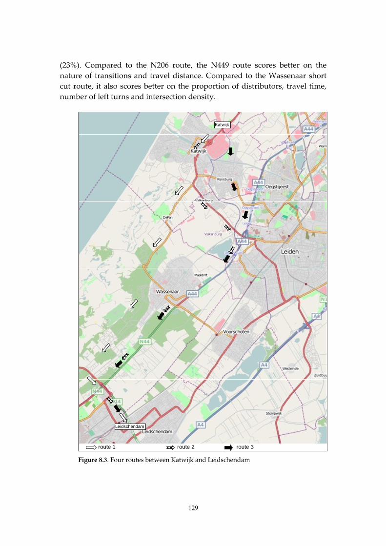
129
(23%). Compared to the N206 route, the N449 route scores better on the
nature of transitions and travel distance. Compared to the Wassenaar short
cut route, it also scores better on the proportion of distributors, travel time,
number of left turns and intersection density.
route 1 route 2 route 3
Leidschendam
Katwijk
Figure 8.3. Four routes between Katwijk and Leidschendam

130
Cr. Description Weight gc Wassenaar
short cut
N206 ‐ A44
‐ N44
N449 ‐ A44
‐ N44
1 Number of transitions 0.111 1 1 1
2 Nature of transitions 0.111 1 1 0
3 Missing road categories 0.111 1 1 1
4 Proportion of access roads 0.111 0.0 0.0 0.0
5 Proportion of distributors 0.111 92.4 64.7 69.8
6 Travel distance [kilometres] 0.111 17.0 18.4 17.2
7 Travel time [minutes] 0.111 23.0 19.0 19.0
8 Left turns 0.111 2.0 1.0 1.0
9 Junction density (per km) 0.111 1.9 0.4 1.2
Sum 1.000
Table 8.6. Scores Cji for four routes between Katwijk and Leidschendam
For this OD pair, the fastest routes are also the routes with the highest DV
scores. Figure 8.4 depicts the route stars of these three routes. Obviously, the
bottom left figure represents the best route.
No. Description of alternative Wassenaar
short cut
N206 ‐
A44 ‐ N44
N449 ‐
A44 ‐ N44
OD score
1 See Table 8.6 44 78 91 68
2 Weights according to Table 8.3 27 89 88 65
3 No. 1 and alt. distribution of
traffic
44 78 91 73
4 No. 1 and alt. travel time 56 78 80 70
Table 8.7. DV scores and OD scores for each alternative
Table 8.7 contains the results of calculations regarding three sets of
assumptions. First, the weights are chosen according to Table 8.3. Applying
these weights, changes the DV scores substantially (Table 8.7, row No. 2). The
score of the Wassenaar short cut route decreases (from 44 to 27) while the
scores of the other two routes hardly differ anymore (from a difference of 13
to only 1). The OD score does not change very much: the improvement of
one route (N206) and the ʹdeclineʹ (Wassenaar) of another route cancel each
other out.
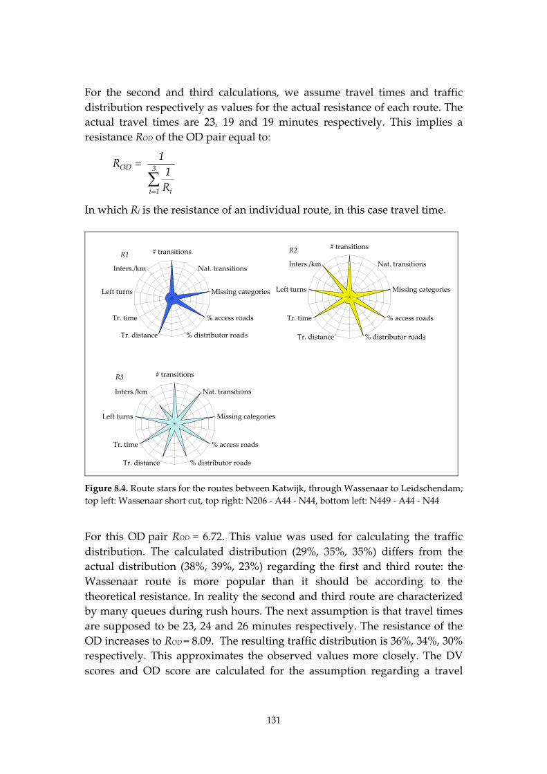
131
R2
-0.2
0
0.2
0.4
0.6
0.8
1
# transitions
Nat. transitions
Missing categories
% access roads
% distributor roadsTr. distance
Tr. time
Left turns
Inters./km
R1
-0.2
0
0.2
0.4
0.6
0.8
1
# transitions
Nat. transitions
Missing categories
% access roads
% distributor roadsTr. distance
Tr. time
Left turns
Inters./km
R3
-0.2
0
0.2
0.4
0.6
0.8
1
# transitions
Nat. transitions
Missing categories
% access roads
% distributor roadsTr. distance
Tr. time
Left turns
Inters./km
For the second and third calculations, we assume travel times and traffic
distribution respectively as values for the actual resistance of each route. The
actual travel times are 23, 19 and 19 minutes respectively. This implies a
resistance ROD of the OD pair equal to:
3
1i i
OD
R
1
1R
In which Ri is the resistance of an individual route, in this case travel time.
Figure 8.4. Route stars for the routes between Katwijk, through Wassenaar to Leidschendam;
top left: Wassenaar short cut, top right: N206 ‐ A44 ‐ N44, bottom left: N449 ‐ A44 ‐ N44
For this OD pair ROD = 6.72. This value was used for calculating the traffic
distribution. The calculated distribution (29%, 35%, 35%) differs from the
actual distribution (38%, 39%, 23%) regarding the first and third route: the
Wassenaar route is more popular than it should be according to the
theoretical resistance. In reality the second and third route are characterized
by many queues during rush hours. The next assumption is that travel times
are supposed to be 23, 24 and 26 minutes respectively. The resistance of the
OD increases to ROD = 8.09. The resulting traffic distribution is 36%, 34%, 30%
respectively. This approximates the observed values more closely. The DV
scores and OD score are calculated for the assumption regarding a travel
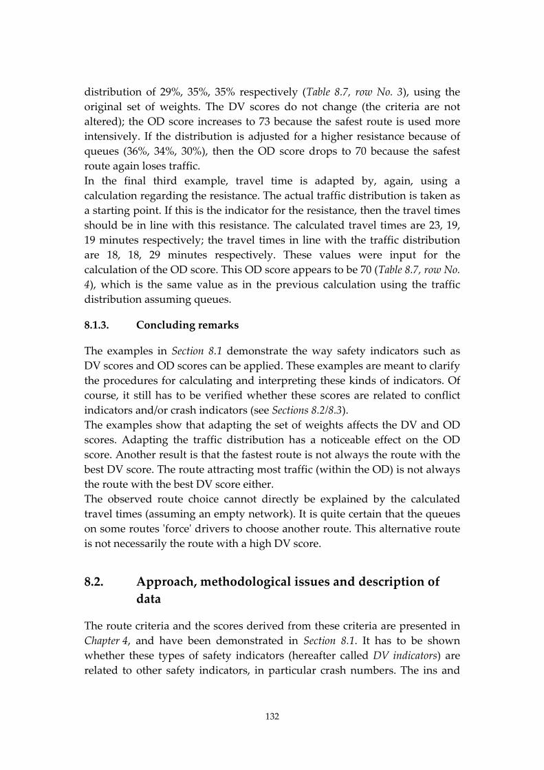
132
distribution of 29%, 35%, 35% respectively (Table 8.7, row No. 3), using the
original set of weights. The DV scores do not change (the criteria are not
altered); the OD score increases to 73 because the safest route is used more
intensively. If the distribution is adjusted for a higher resistance because of
queues (36%, 34%, 30%), then the OD score drops to 70 because the safest
route again loses traffic.
In the final third example, travel time is adapted by, again, using a
calculation regarding the resistance. The actual traffic distribution is taken as
a starting point. If this is the indicator for the resistance, then the travel times
should be in line with this resistance. The calculated travel times are 23, 19,
19 minutes respectively; the travel times in line with the traffic distribution
are 18, 18, 29 minutes respectively. These values were input for the
calculation of the OD score. This OD score appears to be 70 (Table 8.7, row No.
4), which is the same value as in the previous calculation using the traffic
distribution assuming queues.
8.1.3. Concluding remarks
The examples in Section 8.1 demonstrate the way safety indicators such as
DV scores and OD scores can be applied. These examples are meant to clarify
the procedures for calculating and interpreting these kinds of indicators. Of
course, it still has to be verified whether these scores are related to conflict
indicators and/or crash indicators (see Sections 8.2/8.3).
The examples show that adapting the set of weights affects the DV and OD
scores. Adapting the traffic distribution has a noticeable effect on the OD
score. Another result is that the fastest route is not always the route with the
best DV score. The route attracting most traffic (within the OD) is not always
the route with the best DV score either.
The observed route choice cannot directly be explained by the calculated
travel times (assuming an empty network). It is quite certain that the queues
on some routes ʹforceʹ drivers to choose another route. This alternative route
is not necessarily the route with a high DV score.
8.2. Approach, methodological issues and description of
data
The route criteria and the scores derived from these criteria are presented in
Chapter 4, and have been demonstrated in Section 8.1. It has to be shown
whether these types of safety indicators (hereafter called DV indicators) are
related to other safety indicators, in particular crash numbers. The ins and
133
outs of the quantitative relationships between crash numbers and conflict
numbers were shown in Section 7.2. Showing a direct relationship between
crash numbers and DV indicators in a similar way is hardly possible. That is
because the crash numbers for individual routes are very insignificant: solid
quantitative relationships can therefore not be established. To bypass this
problem, the relationships between conflict numbers and DV indicators will
be examined. If these types of relationships appear to be strong, then the
existence of a relationship between DV indicators and crash numbers is
plausible.
The data about DV indicators and other route characteristics will also be
used to analyse general assumptions regarding the safety of routes and route
choice.
This section will deal with describing the data (sets), formulating hypotheses,
and discussing some methodological issues.
8.2.1. Description of the data
Some of the data are the output of the micro‐simulation model: these
(dynamic) data are the averages of ten runs. They are data about the number
of vehicles per route and per road section, the vehicle movements (in
particular near intersections), the actual travel times, the departure and
arrival times, and the driving speeds. The other data have been calculated
using the previous data as input; Table 8.8a and 8.8b show these ʹotherʹ data.
The conflicts on the intersections can be divided into frontal, longitudinal
(rear‐end), transversal (lateral), and converging conflicts (Section 6.4, Figure
6.8). For the analysis, it is relevant to focus on conflicts that involve vehicles
following the route. For a transversal (lateral) conflict, it is always certain
that one of the vehicles is following the route to be analysed. For this reason,
the following analyses will be limited to these lateral conflicts.
Variable name Description
Origin Identification number of Origin zone
Destination Identification number of Destination zone
Volledig Are Origin and Destination both within the study area?
NRoutes Number of routes (being used) within the OD
DVtotaal DV score (Formula 6.3)
DVtotaalSTD Standardized DV score (Formula 6.9)
Table 8.8a. Variables regarding OD pairs
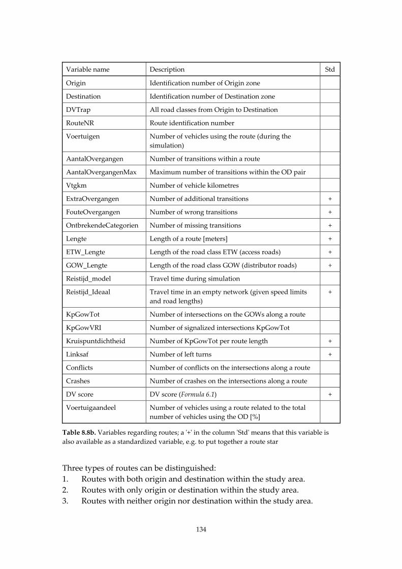
134
Variable name Description Std
Origin Identification number of Origin zone
Destination Identification number of Destination zone
DVTrap All road classes from Origin to Destination
RouteNR Route identification number
Voertuigen Number of vehicles using the route (during the
simulation)
AantalOvergangen Number of transitions within a route
AantalOvergangenMax Maximum number of transitions within the OD pair
Vtgkm Number of vehicle kilometres
ExtraOvergangen Number of additional transitions +
FouteOvergangen Number of wrong transitions +
OntbrekendeCategorien Number of missing transitions +
Lengte Length of a route [meters] +
ETW_Lengte Length of the road class ETW (access roads) +
GOW_Lengte Length of the road class GOW (distributor roads) +
Reistijd_model Travel time during simulation
Reistijd_Ideaal Travel time in an empty network (given speed limits
and road lengths)
+
KpGowTot Number of intersections on the GOWs along a route
KpGowVRI Number of signalized intersections KpGowTot
Kruispuntdichtheid Number of KpGowTot per route length +
Linksaf Number of left turns +
Conflicts Number of conflicts on the intersections along a route
Crashes Number of crashes on the intersections along a route
DV score DV score (Formula 6.1) +
Voertuigaandeel Number of vehicles using a route related to the total
number of vehicles using the OD [%]
Table 8.8b. Variables regarding routes; a ʹ+ʹ in the column ʹStdʹ means that this variable is
also available as a standardized variable, e.g. to put together a route star
Three types of routes can be distinguished:
1. Routes with both origin and destination within the study area.
2. Routes with only origin or destination within the study area.
3. Routes with neither origin nor destination within the study area.
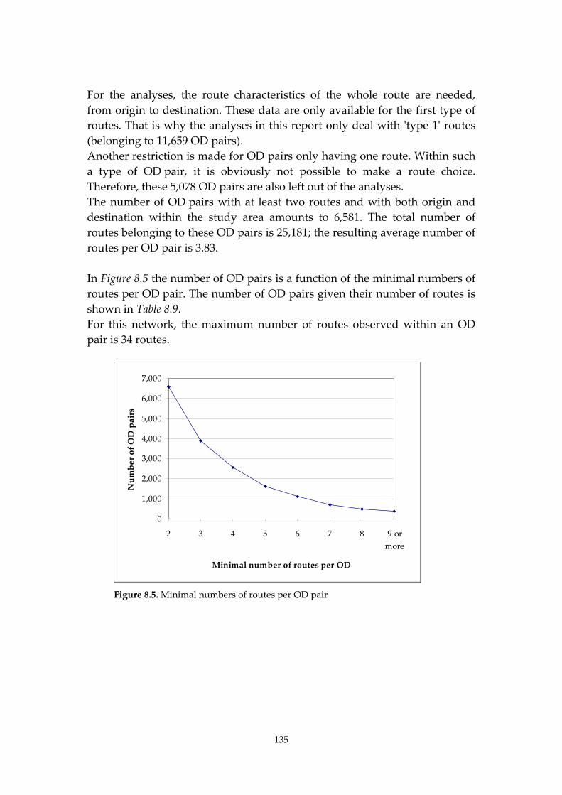
135
For the analyses, the route characteristics of the whole route are needed,
from origin to destination. These data are only available for the first type of
routes. That is why the analyses in this report only deal with ʹtype 1ʹ routes
(belonging to 11,659 OD pairs).
Another restriction is made for OD pairs only having one route. Within such
a type of OD pair, it is obviously not possible to make a route choice.
Therefore, these 5,078 OD pairs are also left out of the analyses.
The number of OD pairs with at least two routes and with both origin and
destination within the study area amounts to 6,581. The total number of
routes belonging to these OD pairs is 25,181; the resulting average number of
routes per OD pair is 3.83.
In Figure 8.5 the number of OD pairs is a function of the minimal numbers of
routes per OD pair. The number of OD pairs given their number of routes is
shown in Table 8.9.
For this network, the maximum number of routes observed within an OD
pair is 34 routes.
0
1,000
2,000
3,000
4,000
5,000
6,000
7,000
2 3 4 5 6 7 8 9 or
more
Minimal number of routes per OD
Number of OD pairs
Figure 8.5. Minimal numbers of routes per OD pair
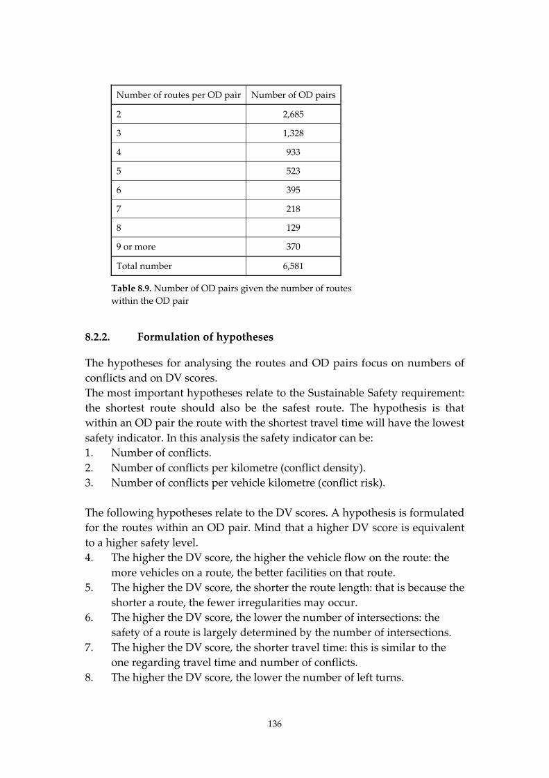
136
Number of routes per OD pair Number of OD pairs
2 2,685
3 1,328
4 933
5 523
6 395
7 218
8 129
9 or more 370
Total number 6,581
Table 8.9. Number of OD pairs given the number of routes
within the OD pair
8.2.2. Formulation of hypotheses
The hypotheses for analysing the routes and OD pairs focus on numbers of
conflicts and on DV scores.
The most important hypotheses relate to the Sustainable Safety requirement:
the shortest route should also be the safest route. The hypothesis is that
within an OD pair the route with the shortest travel time will have the lowest
safety indicator. In this analysis the safety indicator can be:
1. Number of conflicts.
2. Number of conflicts per kilometre (conflict density).
3. Number of conflicts per vehicle kilometre (conflict risk).
The following hypotheses relate to the DV scores. A hypothesis is formulated
for the routes within an OD pair. Mind that a higher DV score is equivalent
to a higher safety level.
4. The higher the DV score, the higher the vehicle flow on the route: the
more vehicles on a route, the better facilities on that route.
5. The higher the DV score, the shorter the route length: that is because the
shorter a route, the fewer irregularities may occur.
6. The higher the DV score, the lower the number of intersections: the
safety of a route is largely determined by the number of intersections.
7. The higher the DV score, the shorter travel time: this is similar to the
one regarding travel time and number of conflicts.
8. The higher the DV score, the lower the number of left turns.
137
9. The higher the DV score, the lower the number of intersections per
kilometre:
10. The higher the DV score, the lower the number of conflicts.
11. The higher the DV score, the lower the number of conflicts per
kilometre.
12. The higher the DV score, the lower the number of conflicts per vehicle
kilometre.
The routes differ in length: the shortest route amounts to 62 metres (!), the
longest one to 23.9 kilometres. The shorter routes may differ from the longer
ones, since they might miss essential route characteristics. Therefore, the next
hypothesis is:
13. Hypothesis 10 can best be tested for longer routes instead of all 25,181
routes.
These thirteen hypotheses will be tested according to a procedure explained
in Section 8.2.4.
8.2.3. Varying the DV scores
The DV scores for the hypotheses in Section 8.2.2 are calculated according to
Formula 6.8, using equal weights for all criteria. However, it is very likely that
the criteria are not equally important regarding their relationship with the
safety indicators. That is why a series of DV scores will be tested. These DV
scores are listed in Table 8.10. The scores DV1 to DV7 are meant to test
whether the systematic addition of a criterion gradually produces a better
result. DV8 and DV9 are intended to test the assumption that the number of
left turns and the intersection density are strongly related to the conflict
indicators. The wghDV score was introduced in Section 8.1.
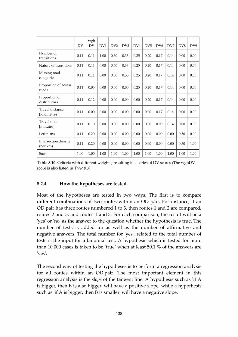
138
DV
wgh
DV DV1 DV2 DV3 DV4 DV5 DV6 DV7 DV8 DV9
Number of
transitions 0,11 0.11 1.00 0.50 0.33 0.25 0.20 0.17 0.14 0.00 0.00
Nature of transitions 0,11 0.11 0.00 0.50 0.33 0.25 0.20 0.17 0.14 0.00 0.00
Missing road
categories 0,11 0.11 0.00 0.00 0.33 0.25 0.20 0.17 0.14 0.00 0.00
Proportion of access
roads 0,11 0.05 0.00 0.00 0.00 0.25 0.20 0.17 0.14 0.00 0.00
Proportion of
distributors 0,11 0.12 0.00 0.00 0.00 0.00 0.20 0.17 0.14 0.00 0.00
Travel distance
[kilometres] 0,11 0.00 0.00 0.00 0.00 0.00 0.00 0.17 0.14 0.00 0.00
Travel time
[minutes] 0,11 0.10 0.00 0.00 0.00 0.00 0.00 0.00 0.14 0.00 0.00
Left turns 0,11 0.20 0.00 0.00 0.00 0.00 0.00 0.00 0.00 0.50 0.00
Intersection density
(per km) 0,11 0.20 0.00 0.00 0.00 0.00 0.00 0.00 0.00 0.50 1.00
Sum 1.00 1.00 1.00 1.00 1.00 1.00 1.00 1.00 1.00 1.00 1.00
Table 8.10. Criteria with different weights, resulting in a series of DV scores (The wghDV
score is also listed in Table 8.3)
8.2.4. How the hypotheses are tested
Most of the hypotheses are tested in two ways. The first is to compare
different combinations of two routes within an OD pair. For instance, if an
OD pair has three routes numbered 1 to 3, then routes 1 and 2 are compared,
routes 2 and 3, and routes 1 and 3. For each comparison, the result will be a
ʹyesʹ or ʹnoʹ as the answer to the question whether the hypothesis is true. The
number of tests is added up as well as the number of affirmative and
negative answers. The total number for ʹyesʹ, related to the total number of
tests is the input for a binomial test. A hypothesis which is tested for more
than 10,000 cases is taken to be ‘true’ when at least 50.1 % of the answers are
ʹyesʹ.
The second way of testing the hypotheses is to perform a regression analysis
for all routes within an OD pair. The most important element in this
regression analysis is the slope of the tangent line. A hypothesis such as ʹif A
is bigger, then B is also biggerʹ will have a positive slope, while a hypothesis
such as ʹif A is bigger, then B is smallerʹ will have a negative slope.
139
These regression analyses are applied to the OD pairs having a maximum of
eight routes. The remaining 370 OD pairs (with nine or more routes) are put
aside because their contribution to the total result will be small while the
calculation procedure will become more and more complicated.
Again, the hypothesis is true when the number of negative or positive slopes
(depending on the type of hypothesis) related to the total number of tested
OD pairs is more than 50.1%.
The first way of testing is applied to all hypotheses; the second way is
applied to a selected number of hypotheses.
8.3. Analysing scores, numbers of conflicts, and travel
times
The hypotheses formulated in Section 8.2 will be tested below, by pair‐wise
comparisons first, followed by the regression analyses.
8.3.1. Pair‐wise comparisons
The pair‐wise comparisons are meant to gain a clear insight into the mutual
relationships between the routes within an OD pair. Not all routes within an
OD pair are compared to each other. The comparisons are structured
according to the system in Table 8.11: consecutive routes (i+1 and i) are
compared to each other as well as routes i+2 and i (i ≤ 9). This limitation has a
merely practical motivation: to reduce the number of operations. However,
this approach still results in many comparisons, more than enough for
executing the binomial tests satisfactorily.
A methodological drawback to this procedure regards routes that are
included in two or more tests. This can be observed in Table 8.11: e.g., route 1
(in OD pair A ‐B) is involved in two tests. Therefore, these tests are not
considered completely independent. To check the effect of this dependency,
the sequence of the routes within an OD pair was randomly changed in some
tests (at the end of Section 8.3.1).
A second drawback regards routes that have some road sections in common:
the overlapping of routes. This will also harm the assumption of
independency in a statistical test. On the other hand, from a traffic and
transport point of view the entire route has to be considered instead of only
part of it. Although consideration of a shorter part may result in the desired
independency (of another part of another route), the essence of the route
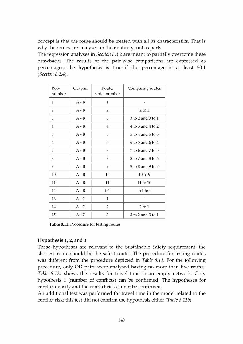
140
concept is that the route should be treated with all its characteristics. That is
why the routes are analysed in their entirety, not as parts.
The regression analyses in Section 8.3.2 are meant to partially overcome these
drawbacks. The results of the pair‐wise comparisons are expressed as
percentages; the hypothesis is true if the percentage is at least 50.1
(Section 8.2.4).
Row
number
OD pair Route,
serial number
Comparing routes
1 A ‐ B 1 ‐
2 A ‐ B 2 2 to 1
3 A ‐ B 3 3 to 2 and 3 to 1
4 A ‐ B 4 4 to 3 and 4 to 2
5 A ‐ B 5 5 to 4 and 5 to 3
6 A ‐ B 6 6 to 5 and 6 to 4
7 A ‐ B 7 7 to 6 and 7 to 5
8 A ‐ B 8 8 to 7 and 8 to 6
9 A ‐ B 9 9 to 8 and 9 to 7
10 A ‐ B 10 10 to 9
11 A ‐ B 11 11 to 10
12 A ‐ B i+1 i+1 to i
13 A ‐ C 1 ‐
14 A ‐ C 2 2 to 1
15 A ‐ C 3 3 to 2 and 3 to 1
Table 8.11. Procedure for testing routes
Hypothesis 1, 2, and 3
These hypotheses are relevant to the Sustainable Safety requirement ʹthe
shortest route should be the safest routeʹ. The procedure for testing routes
was different from the procedure depicted in Table 8.11. For the following
procedure, only OD pairs were analysed having no more than five routes.
Table 8.12a shows the results for travel time in an empty network. Only
hypothesis 1 (number of conflicts) can be confirmed. The hypotheses for
conflict density and the conflict risk cannot be confirmed.
An additional test was performed for travel time in the model related to the
conflict risk; this test did not confirm the hypothesis either (Table 8.12b).
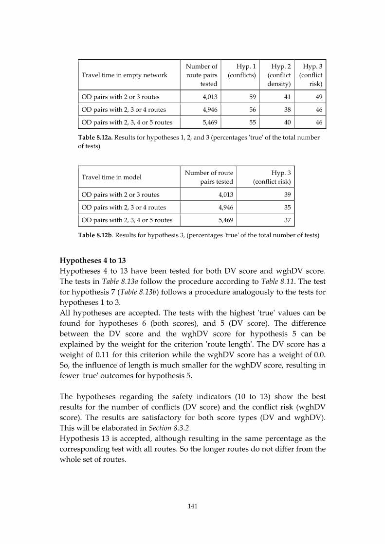
141
Travel time in empty network
Number of
route pairs
tested
Hyp. 1
(conflicts)
Hyp. 2
(conflict
density)
Hyp. 3
(conflict
risk)
OD pairs with 2 or 3 routes 4,013 59 41 49
OD pairs with 2, 3 or 4 routes 4,946 56 38 46
OD pairs with 2, 3, 4 or 5 routes 5,469 55 40 46
Table 8.12a. Results for hypotheses 1, 2, and 3 (percentages ʹtrueʹ of the total number
of tests)
Travel time in model Number of route
pairs tested
Hyp. 3
(conflict risk)
OD pairs with 2 or 3 routes 4,013 39
OD pairs with 2, 3 or 4 routes 4,946 35
OD pairs with 2, 3, 4 or 5 routes 5,469 37
Table 8.12b. Results for hypothesis 3, (percentages ʹtrueʹ of the total number of tests)
Hypotheses 4 to 13
Hypotheses 4 to 13 have been tested for both DV score and wghDV score.
The tests in Table 8.13a follow the procedure according to Table 8.11. The test
for hypothesis 7 (Table 8.13b) follows a procedure analogously to the tests for
hypotheses 1 to 3.
All hypotheses are accepted. The tests with the highest ʹtrueʹ values can be
found for hypotheses 6 (both scores), and 5 (DV score). The difference
between the DV score and the wghDV score for hypothesis 5 can be
explained by the weight for the criterion ʹroute lengthʹ. The DV score has a
weight of 0.11 for this criterion while the wghDV score has a weight of 0.0.
So, the influence of length is much smaller for the wghDV score, resulting in
fewer ʹtrueʹ outcomes for hypothesis 5.
The hypotheses regarding the safety indicators (10 to 13) show the best
results for the number of conflicts (DV score) and the conflict risk (wghDV
score). The results are satisfactory for both score types (DV and wghDV).
This will be elaborated in Section 8.3.2.
Hypothesis 13 is accepted, although resulting in the same percentage as the
corresponding test with all routes. So the longer routes do not differ from the
whole set of routes.
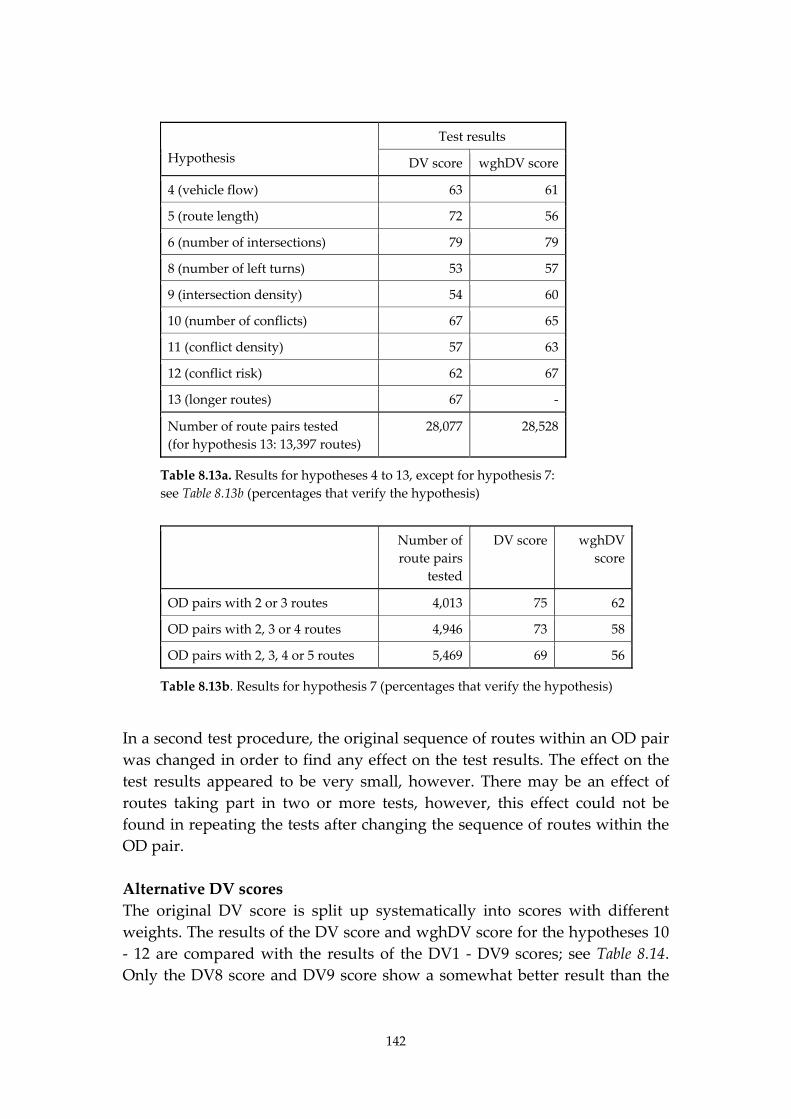
142
Test results
Hypothesis DV score wghDV score
4 (vehicle flow) 63 61
5 (route length) 72 56
6 (number of intersections) 79 79
8 (number of left turns) 53 57
9 (intersection density) 54 60
10 (number of conflicts) 67 65
11 (conflict density) 57 63
12 (conflict risk) 62 67
13 (longer routes) 67 ‐
Number of route pairs tested
(for hypothesis 13: 13,397 routes)
28,077 28,528
Table 8.13a. Results for hypotheses 4 to 13, except for hypothesis 7:
see Table 8.13b (percentages that verify the hypothesis)
Number of
route pairs
tested
DV score wghDV
score
OD pairs with 2 or 3 routes 4,013 75 62
OD pairs with 2, 3 or 4 routes 4,946 73 58
OD pairs with 2, 3, 4 or 5 routes 5,469 69 56
Table 8.13b. Results for hypothesis 7 (percentages that verify the hypothesis)
In a second test procedure, the original sequence of routes within an OD pair
was changed in order to find any effect on the test results. The effect on the
test results appeared to be very small, however. There may be an effect of
routes taking part in two or more tests, however, this effect could not be
found in repeating the tests after changing the sequence of routes within the
OD pair.
Alternative DV scores
The original DV score is split up systematically into scores with different
weights. The results of the DV score and wghDV score for the hypotheses 10
‐ 12 are compared with the results of the DV1 ‐ DV9 scores; see Table 8.14.
Only the DV8 score and DV9 score show a somewhat better result than the
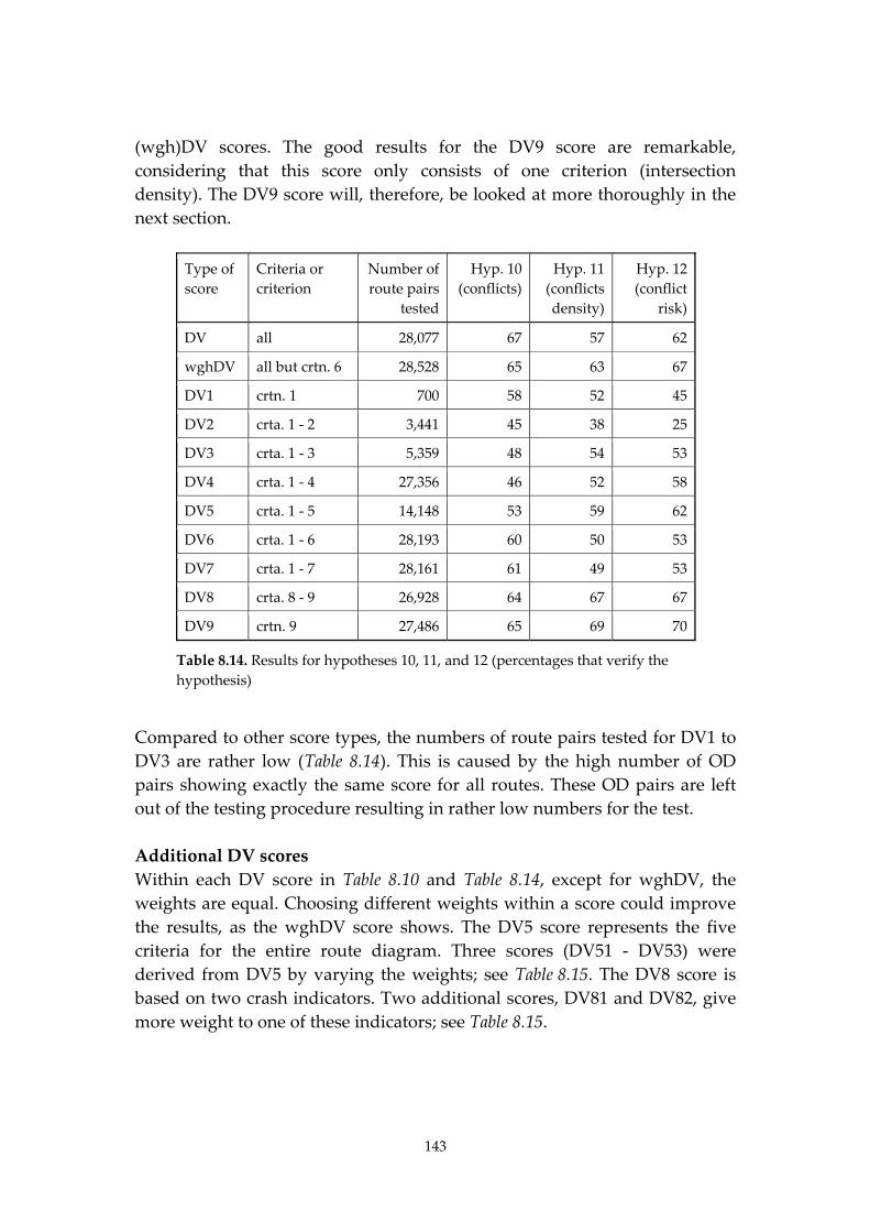
143
(wgh)DV scores. The good results for the DV9 score are remarkable,
considering that this score only consists of one criterion (intersection
density). The DV9 score will, therefore, be looked at more thoroughly in the
next section.
Type of
score
Criteria or
criterion
Number of
route pairs
tested
Hyp. 10
(conflicts)
Hyp. 11
(conflicts
density)
Hyp. 12
(conflict
risk)
DV all 28,077 67 57 62
wghDV all but crtn. 6 28,528 65 63 67
DV1 crtn. 1 700 58 52 45
DV2 crta. 1 ‐ 2 3,441 45 38 25
DV3 crta. 1 ‐ 3 5,359 48 54 53
DV4 crta. 1 ‐ 4 27,356 46 52 58
DV5 crta. 1 ‐ 5 14,148 53 59 62
DV6 crta. 1 ‐ 6 28,193 60 50 53
DV7 crta. 1 ‐ 7 28,161 61 49 53
DV8 crta. 8 ‐ 9 26,928 64 67 67
DV9 crtn. 9 27,486 65 69 70
Table 8.14. Results for hypotheses 10, 11, and 12 (percentages that verify the
hypothesis)
Compared to other score types, the numbers of route pairs tested for DV1 to
DV3 are rather low (Table 8.14). This is caused by the high number of OD
pairs showing exactly the same score for all routes. These OD pairs are left
out of the testing procedure resulting in rather low numbers for the test.
Additional DV scores
Within each DV score in Table 8.10 and Table 8.14, except for wghDV, the
weights are equal. Choosing different weights within a score could improve
the results, as the wghDV score shows. The DV5 score represents the five
criteria for the entire route diagram. Three scores (DV51 ‐ DV53) were
derived from DV5 by varying the weights; see Table 8.15. The DV8 score is
based on two crash indicators. Two additional scores, DV81 and DV82, give
more weight to one of these indicators; see Table 8.15.
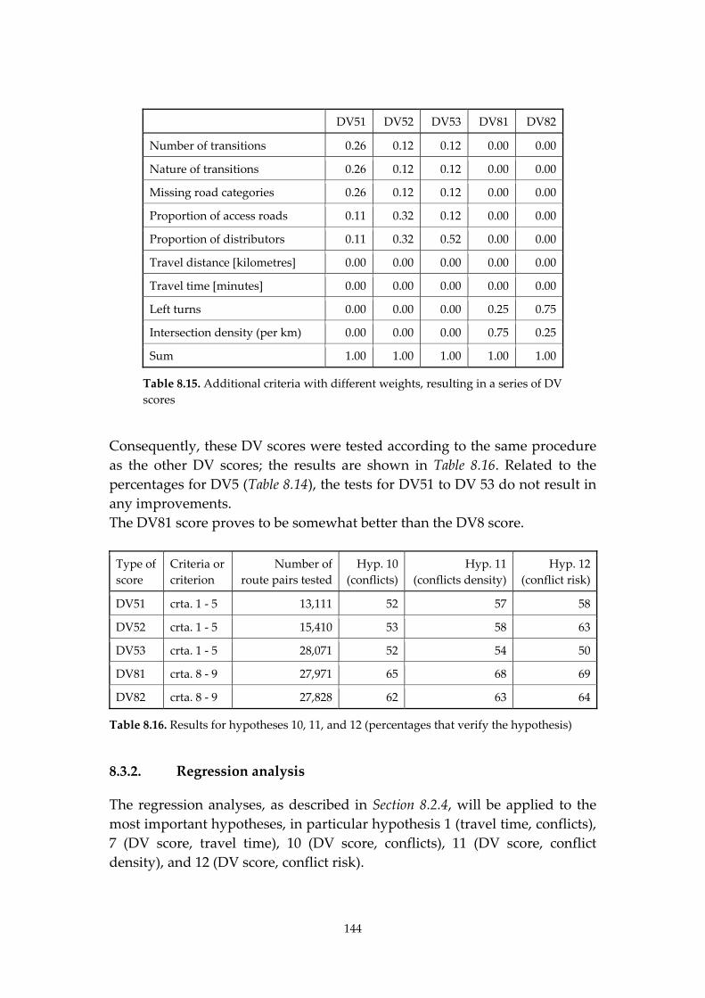
144
DV51 DV52 DV53 DV81 DV82
Number of transitions 0.26 0.12 0.12 0.00 0.00
Nature of transitions 0.26 0.12 0.12 0.00 0.00
Missing road categories 0.26 0.12 0.12 0.00 0.00
Proportion of access roads 0.11 0.32 0.12 0.00 0.00
Proportion of distributors 0.11 0.32 0.52 0.00 0.00
Travel distance [kilometres] 0.00 0.00 0.00 0.00 0.00
Travel time [minutes] 0.00 0.00 0.00 0.00 0.00
Left turns 0.00 0.00 0.00 0.25 0.75
Intersection density (per km) 0.00 0.00 0.00 0.75 0.25
Sum 1.00 1.00 1.00 1.00 1.00
Table 8.15. Additional criteria with different weights, resulting in a series of DV
scores
Consequently, these DV scores were tested according to the same procedure
as the other DV scores; the results are shown in Table 8.16. Related to the
percentages for DV5 (Table 8.14), the tests for DV51 to DV 53 do not result in
any improvements.
The DV81 score proves to be somewhat better than the DV8 score.
Type of
score
Criteria or
criterion
Number of
route pairs tested
Hyp. 10
(conflicts)
Hyp. 11
(conflicts density)
Hyp. 12
(conflict risk)
DV51 crta. 1 ‐ 5 13,111 52 57 58
DV52 crta. 1 ‐ 5 15,410 53 58 63
DV53 crta. 1 ‐ 5 28,071 52 54 50
DV81 crta. 8 ‐ 9 27,971 65 68 69
DV82 crta. 8 ‐ 9 27,828 62 63 64
Table 8.16. Results for hypotheses 10, 11, and 12 (percentages that verify the hypothesis)
8.3.2. Regression analysis
The regression analyses, as described in Section 8.2.4, will be applied to the
most important hypotheses, in particular hypothesis 1 (travel time, conflicts),
7 (DV score, travel time), 10 (DV score, conflicts), 11 (DV score, conflict
density), and 12 (DV score, conflict risk).

145
Number of routes
within OD pair
Is the slope according
to hypothesis 1?
2 45.8
3 45.2
4 52.5
5 52.6
6 44.6
7 42.2
8 48.1
2 ‐ 8 47.1
Table 8.17a. Variable Travel time in empty network,
results for hypothesis 1
Travel time in empty network and conflicts per unit of length
40.0
42.0
44.0
46.0
48.0
50.0
52.0
54.0
2 3 4 5 6 7 8 9
Number of routes within OD
Pe
rce
nta
ge
or
rou
tes
wit
h a
p
os
itiv
e s
lop
e
Figure 8.6. Percentage of OD pairs with a positive slope, for
different numbers of routes per OD pair
Starting with hypothesis 1, both travel time indicators will be analysed:
ʹtravel time in empty networkʹ and ʹtravel time in modelʹ. Table 8.17a contains
the percentages of OD pairs with a positive slope, for each number of routes
per OD pair. All of these percentages are below 50.0 percent, except for the
OD pairs with four and five routes; see also Figure 8.6.
The analyses for ʹtravel time in modelʹ result in percentages of the same size,
showing only one (six routes) above 50.0 percent (Table 8.17b).
Given these results, the conclusion must be that hypothesis 1 has to be
rejected for both variables. Of course, these are the results for the current
network. Changing the network in the right direction may improve the
results.
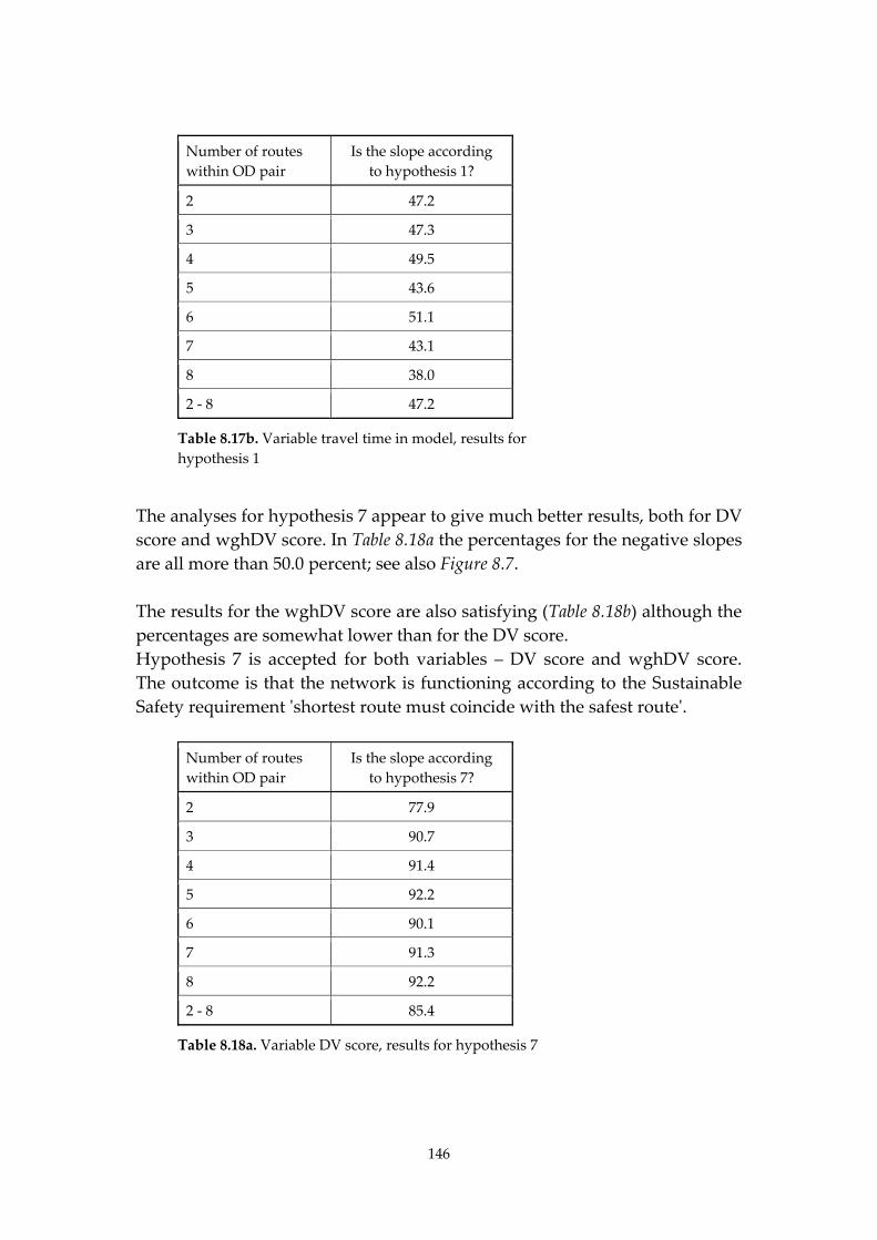
146
Number of routes
within OD pair
Is the slope according
to hypothesis 1?
2 47.2
3 47.3
4 49.5
5 43.6
6 51.1
7 43.1
8 38.0
2 ‐ 8 47.2
Table 8.17b. Variable travel time in model, results for
hypothesis 1
The analyses for hypothesis 7 appear to give much better results, both for DV
score and wghDV score. In Table 8.18a the percentages for the negative slopes
are all more than 50.0 percent; see also Figure 8.7.
The results for the wghDV score are also satisfying (Table 8.18b) although the
percentages are somewhat lower than for the DV score.
Hypothesis 7 is accepted for both variables – DV score and wghDV score.
The outcome is that the network is functioning according to the Sustainable
Safety requirement ʹshortest route must coincide with the safest routeʹ.
Number of routes
within OD pair
Is the slope according
to hypothesis 7?
2 77.9
3 90.7
4 91.4
5 92.2
6 90.1
7 91.3
8 92.2
2 ‐ 8 85.4
Table 8.18a. Variable DV score, results for hypothesis 7
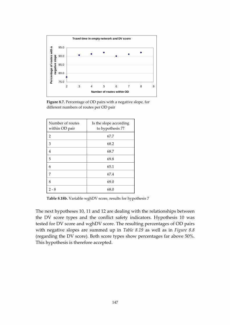
147
Travel time in empty network and DV score
75.0
80.0
85.0
90.0
95.0
2 3 4 5 6 7 8 9
Number of routes within OD
Pe
rce
nta
ge
of
rou
tes
wit
h a
n
eg
ati
ve
slo
pe
Figure 8.7. Percentage of OD pairs with a negative slope, for
different numbers of routes per OD pair
Number of routes
within OD pair
Is the slope according
to hypothesis 7?
2 67.7
3 68.2
4 68.7
5 69.8
6 65.1
7 67.4
8 69.0
2 ‐ 8 68.0
Table 8.18b. Variable wghDV score, results for hypothesis 7
The next hypotheses 10, 11 and 12 are dealing with the relationships between
the DV score types and the conflict safety indicators. Hypothesis 10 was
tested for DV score and wghDV score. The resulting percentages of OD pairs
with negative slopes are summed up in Table 8.19 as well as in Figure 8.8
(regarding the DV score). Both score types show percentages far above 50%.
This hypothesis is therefore accepted.

148
Number of routes
within OD pair
DV score wghDV score
2 61.3 64.3
3 74.8 74.5
4 79.5 77.7
5 80.9 77.1
6 78.0 76.7
7 81.7 79.4
8 81.4 82.9
2 ‐ 8 70.8 71.3
Table 8.19. Results for hypothesis 10 (number of conflicts)
DV score and number of conflicts
60.0
65.0
70.0
75.0
80.0
85.0
2 3 4 5 6 7 8 9
Number of routes within OD
Per
cen
tag
e o
f ro
ute
s w
ith
a
neg
ativ
e sl
op
e
Figure 8.8. Percentage of OD pairs with a negative slope, for
different numbers of routes per OD pair
The results for hypothesis 11 are put into Table 8.20 (DV score and wghDV
score) and Figure 8.9 (DV score). The percentages are above 50 percent,
except for the DV score of an OD pair with two routes. This hypothesis is
accepted as well.
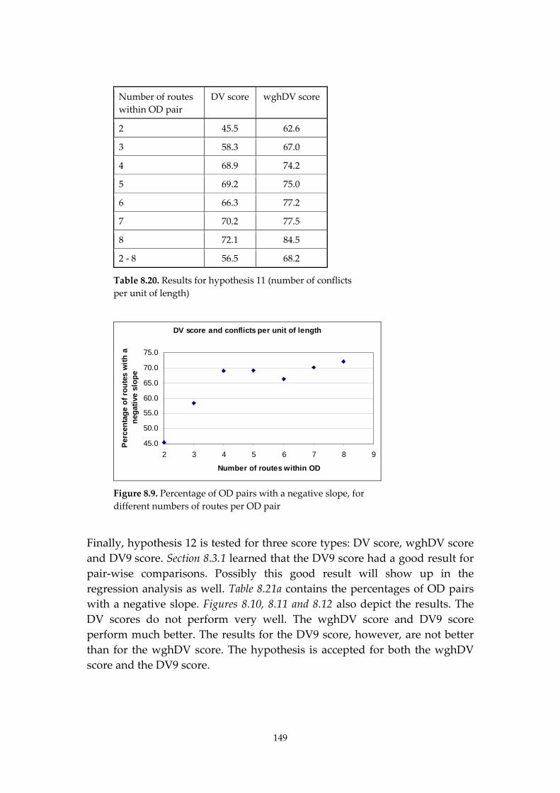
149
Number of routes
within OD pair
DV score wghDV score
2 45.5 62.6
3 58.3 67.0
4 68.9 74.2
5 69.2 75.0
6 66.3 77.2
7 70.2 77.5
8 72.1 84.5
2 ‐ 8 56.5 68.2
Table 8.20. Results for hypothesis 11 (number of conflicts
per unit of length)
DV score and conflicts per unit of length
45.0
50.0
55.0
60.0
65.0
70.0
75.0
2 3 4 5 6 7 8 9
Number of routes within OD
Per
cen
tag
e o
f ro
ute
s w
ith
a
neg
ativ
e sl
op
e
Figure 8.9. Percentage of OD pairs with a negative slope, for
different numbers of routes per OD pair
Finally, hypothesis 12 is tested for three score types: DV score, wghDV score
and DV9 score. Section 8.3.1 learned that the DV9 score had a good result for
pair‐wise comparisons. Possibly this good result will show up in the
regression analysis as well. Table 8.21a contains the percentages of OD pairs
with a negative slope. Figures 8.10, 8.11 and 8.12 also depict the results. The
DV scores do not perform very well. The wghDV score and DV9 score
perform much better. The results for the DV9 score, however, are not better
than for the wghDV score. The hypothesis is accepted for both the wghDV
score and the DV9 score.
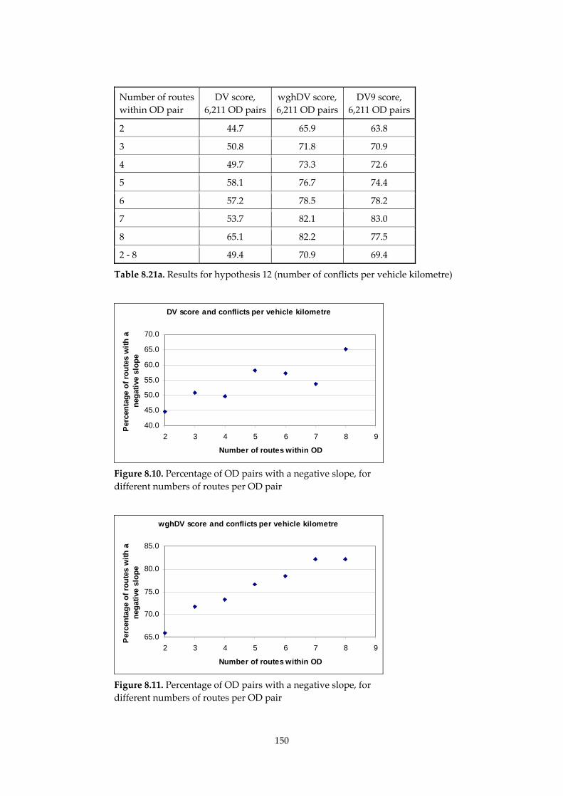
150
Number of routes
within OD pair
DV score,
6,211 OD pairs
wghDV score,
6,211 OD pairs
DV9 score,
6,211 OD pairs
2 44.7 65.9 63.8
3 50.8 71.8 70.9
4 49.7 73.3 72.6
5 58.1 76.7 74.4
6 57.2 78.5 78.2
7 53.7 82.1 83.0
8 65.1 82.2 77.5
2 ‐ 8 49.4 70.9 69.4
Table 8.21a. Results for hypothesis 12 (number of conflicts per vehicle kilometre)
DV score and conflicts per vehicle kilometre
40.0
45.0
50.0
55.0
60.0
65.0
70.0
2 3 4 5 6 7 8 9
Number of routes within OD
Per
cen
tag
e o
f ro
ute
s w
ith
a
neg
ativ
e sl
op
e
Figure 8.10. Percentage of OD pairs with a negative slope, for
different numbers of routes per OD pair
wghDV score and conflicts per vehicle kilometre
65.0
70.0
75.0
80.0
85.0
2 3 4 5 6 7 8 9
Number of routes within OD
Per
cen
tag
e o
f ro
ute
s w
ith
a
neg
ativ
e sl
op
e
Figure 8.11. Percentage of OD pairs with a negative slope, for
different numbers of routes per OD pair
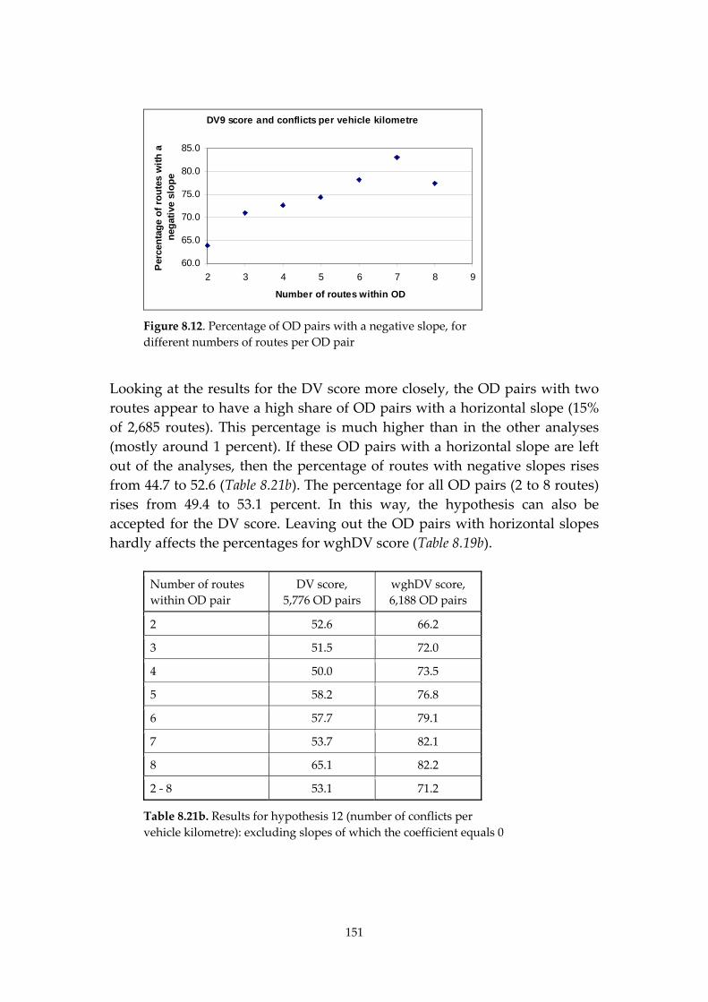
151
DV9 score and conflicts per vehicle kilometre
60.0
65.0
70.0
75.0
80.0
85.0
2 3 4 5 6 7 8 9
Number of routes within OD
Per
cen
tag
e o
f ro
ute
s w
ith
a
neg
ativ
e sl
op
e
Figure 8.12. Percentage of OD pairs with a negative slope, for
different numbers of routes per OD pair
Looking at the results for the DV score more closely, the OD pairs with two
routes appear to have a high share of OD pairs with a horizontal slope (15%
of 2,685 routes). This percentage is much higher than in the other analyses
(mostly around 1 percent). If these OD pairs with a horizontal slope are left
out of the analyses, then the percentage of routes with negative slopes rises
from 44.7 to 52.6 (Table 8.21b). The percentage for all OD pairs (2 to 8 routes)
rises from 49.4 to 53.1 percent. In this way, the hypothesis can also be
accepted for the DV score. Leaving out the OD pairs with horizontal slopes
hardly affects the percentages for wghDV score (Table 8.19b).
Number of routes
within OD pair
DV score,
5,776 OD pairs
wghDV score,
6,188 OD pairs
2 52.6 66.2
3 51.5 72.0
4 50.0 73.5
5 58.2 76.8
6 57.7 79.1
7 53.7 82.1
8 65.1 82.2
2 ‐ 8 53.1 71.2
Table 8.21b. Results for hypothesis 12 (number of conflicts per
vehicle kilometre): excluding slopes of which the coefficient equals 0
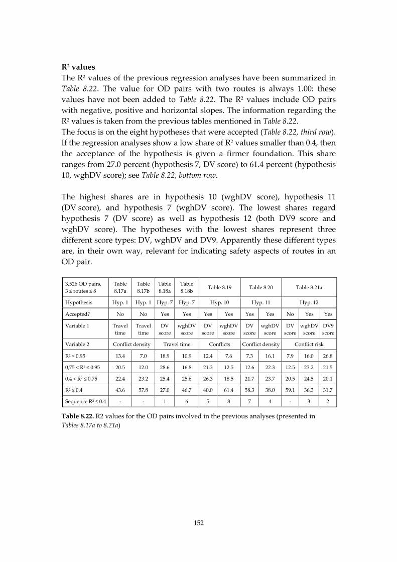
152
R2 values
The R2 values of the previous regression analyses have been summarized in
Table 8.22. The value for OD pairs with two routes is always 1.00: these
values have not been added to Table 8.22. The R2 values include OD pairs
with negative, positive and horizontal slopes. The information regarding the
R2 values is taken from the previous tables mentioned in Table 8.22.
The focus is on the eight hypotheses that were accepted (Table 8.22, third row).
If the regression analyses show a low share of R2 values smaller than 0.4, then
the acceptance of the hypothesis is given a firmer foundation. This share
ranges from 27.0 percent (hypothesis 7, DV score) to 61.4 percent (hypothesis
10, wghDV score); see Table 8.22, bottom row.
The highest shares are in hypothesis 10 (wghDV score), hypothesis 11
(DV score), and hypothesis 7 (wghDV score). The lowest shares regard
hypothesis 7 (DV score) as well as hypothesis 12 (both DV9 score and
wghDV score). The hypotheses with the lowest shares represent three
different score types: DV, wghDV and DV9. Apparently these different types
are, in their own way, relevant for indicating safety aspects of routes in an
OD pair.
3,526 OD pairs,
3 ≤ routes ≤ 8
Table
8.17a
Table
8.17b
Table
8.18a
Table
8.18b Table 8.19 Table 8.20 Table 8.21a
Hypothesis Hyp. 1 Hyp. 1 Hyp. 7 Hyp. 7 Hyp. 10 Hyp. 11 Hyp. 12
Accepted? No No Yes Yes Yes Yes Yes Yes No Yes Yes
Variable 1 Travel
time
Travel
time
DV
score
wghDV
score
DV
score
wghDV
score
DV
score
wghDV
score
DV
score
wghDV
score
DV9
score
Variable 2 Conflict density Travel time Conflicts Conflict density Conflict risk
R2 > 0.95 13.4 7.0 18.9 10.9 12.4 7.6 7.3 16.1 7.9 16.0 26.8
0,75 < R2 ≤ 0.95 20.5 12.0 28.6 16.8 21.3 12.5 12.6 22.3 12.5 23.2 21.5
0.4 < R2 ≤ 0.75 22.4 23.2 25.4 25.6 26.3 18.5 21.7 23.7 20.5 24.5 20.1
R2 ≤ 0.4 43.6 57.8 27.0 46.7 40.0 61.4 58.3 38.0 59.1 36.3 31.7
Sequence R2 ≤ 0.4 ‐ ‐ 1 6 5 8 7 4 ‐ 3 2
Table 8.22. R2 values for the OD pairs involved in the previous analyses (presented in
Tables 8.17a to 8.21a)
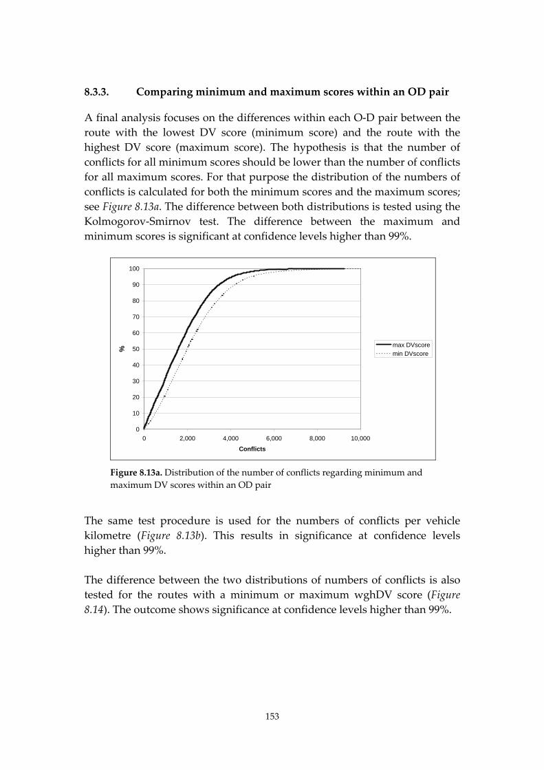
153
8.3.3. Comparing minimum and maximum scores within an OD pair
A final analysis focuses on the differences within each O‐D pair between the
route with the lowest DV score (minimum score) and the route with the
highest DV score (maximum score). The hypothesis is that the number of
conflicts for all minimum scores should be lower than the number of conflicts
for all maximum scores. For that purpose the distribution of the numbers of
conflicts is calculated for both the minimum scores and the maximum scores;
see Figure 8.13a. The difference between both distributions is tested using the
Kolmogorov‐Smirnov test. The difference between the maximum and
minimum scores is significant at confidence levels higher than 99%.
0
10
20
30
40
50
60
70
80
90
100
0 2,000 4,000 6,000 8,000 10,000
Conflicts
%
max DVscoremin DVscore
Figure 8.13a. Distribution of the number of conflicts regarding minimum and
maximum DV scores within an OD pair
The same test procedure is used for the numbers of conflicts per vehicle
kilometre (Figure 8.13b). This results in significance at confidence levels
higher than 99%.
The difference between the two distributions of numbers of conflicts is also
tested for the routes with a minimum or maximum wghDV score (Figure
8.14). The outcome shows significance at confidence levels higher than 99%.
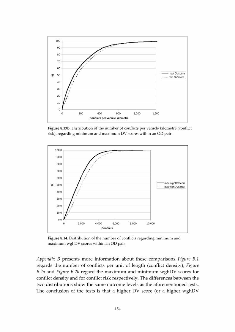
154
0
10
20
30
40
50
60
70
80
90
100
0 300 600 900 1,200 1,500
Conflicts per vehicle kilometre
%
max DVscoremin DVscore
Figure 8.13b. Distribution of the number of conflicts per vehicle kilometre (conflict
risk), regarding minimum and maximum DV scores within an OD pair
0.0
10.0
20.0
30.0
40.0
50.0
60.0
70.0
80.0
90.0
100.0
0 2,000 4,000 6,000 8,000 10,000
Conflicts
%
max wghDVscoremin wghDVscore
Figure 8.14. Distribution of the number of conflicts regarding minimum and
maximum wghDV scores within an OD pair
Appendix B presents more information about these comparisons. Figure B.1
regards the number of conflicts per unit of length (conflict density); Figure
B.2a and Figure B.2b regard the maximum and minimum wghDV scores for
conflict density and for conflict risk respectively. The differences between the
two distributions show the same outcome levels as the aforementioned tests.
The conclusion of the tests is that a higher DV score (or a higher wghDV
155
score) is related to a lower number of conflicts, to a lower conflict density,
and to a lower conflict risk.
8.4. Conclusions
The examples in Section 8.1 demonstrate the way safety indicators such as
DV scores and OD scores can be applied. These examples are meant to clarify
the procedures for calculating and interpreting these kinds of indicators. The
examples show that adapting the set of weights affects the DV and OD
scores. Adapting the traffic distribution has a noticeable effect on the OD
score. Another result is that the fastest route is not always the route with the
best DV score. The route attracting most traffic (within the OD) is not always
the route with the best DV score either.
The observed route choice cannot directly be explained by the calculated
travel times (assuming an empty network). It is quite certain that the queues
on some routes ʹforceʹ drivers to choose another route. This alternative route
is not necessarily the route with a high DV score. Whether the current
network complies with the Sustainable Safety requirement ʹthe shortest route
coincides with the safest routeʹ depends on the safety criterion that is chosen.
The requirement cannot be confirmed when conflict risk or conflict density
are chosen as safety criteria. The opposite is true when the number of
conflicts is taken as the safety criterion. Chapter 10 will show whether
changes in the network will affect traffic volumes and route choice, resulting
in different test results.
An important finding regards the confirmation that both the DV score and
wghDV score relate to the number of conflicts as well as to conflict density
(higher score, fewer conflicts or lower conflict density). The wghDV score
and the DV9 score are both related to conflict risk (higher score, lower risk).
This implies an indirect relationship between the score types and the number
of crashes because the number of conflicts is directly related to the number of
crashes.
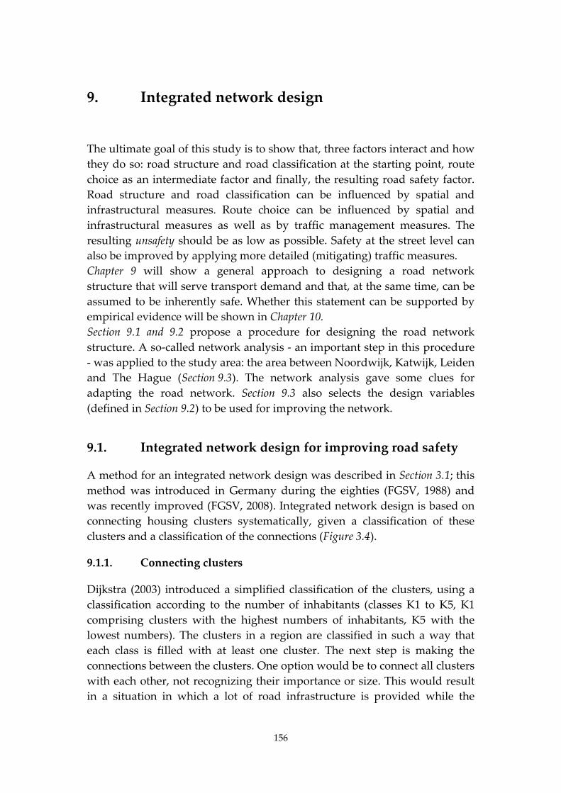
156
9. Integrated network design
The ultimate goal of this study is to show that, three factors interact and how
they do so: road structure and road classification at the starting point, route
choice as an intermediate factor and finally, the resulting road safety factor.
Road structure and road classification can be influenced by spatial and
infrastructural measures. Route choice can be influenced by spatial and
infrastructural measures as well as by traffic management measures. The
resulting unsafety should be as low as possible. Safety at the street level can
also be improved by applying more detailed (mitigating) traffic measures.
Chapter 9 will show a general approach to designing a road network
structure that will serve transport demand and that, at the same time, can be
assumed to be inherently safe. Whether this statement can be supported by
empirical evidence will be shown in Chapter 10.
Section 9.1 and 9.2 propose a procedure for designing the road network
structure. A so‐called network analysis ‐ an important step in this procedure
‐ was applied to the study area: the area between Noordwijk, Katwijk, Leiden
and The Hague (Section 9.3). The network analysis gave some clues for
adapting the road network. Section 9.3 also selects the design variables
(defined in Section 9.2) to be used for improving the network.
9.1. Integrated network design for improving road safety
A method for an integrated network design was described in Section 3.1; this
method was introduced in Germany during the eighties (FGSV, 1988) and
was recently improved (FGSV, 2008). Integrated network design is based on
connecting housing clusters systematically, given a classification of these
clusters and a classification of the connections (Figure 3.4).
9.1.1. Connecting clusters
Dijkstra (2003) introduced a simplified classification of the clusters, using a
classification according to the number of inhabitants (classes K1 to K5, K1
comprising clusters with the highest numbers of inhabitants, K5 with the
lowest numbers). The clusters in a region are classified in such a way that
each class is filled with at least one cluster. The next step is making the
connections between the clusters. One option would be to connect all clusters
with each other, not recognizing their importance or size. This would result
in a situation in which a lot of road infrastructure is provided while the
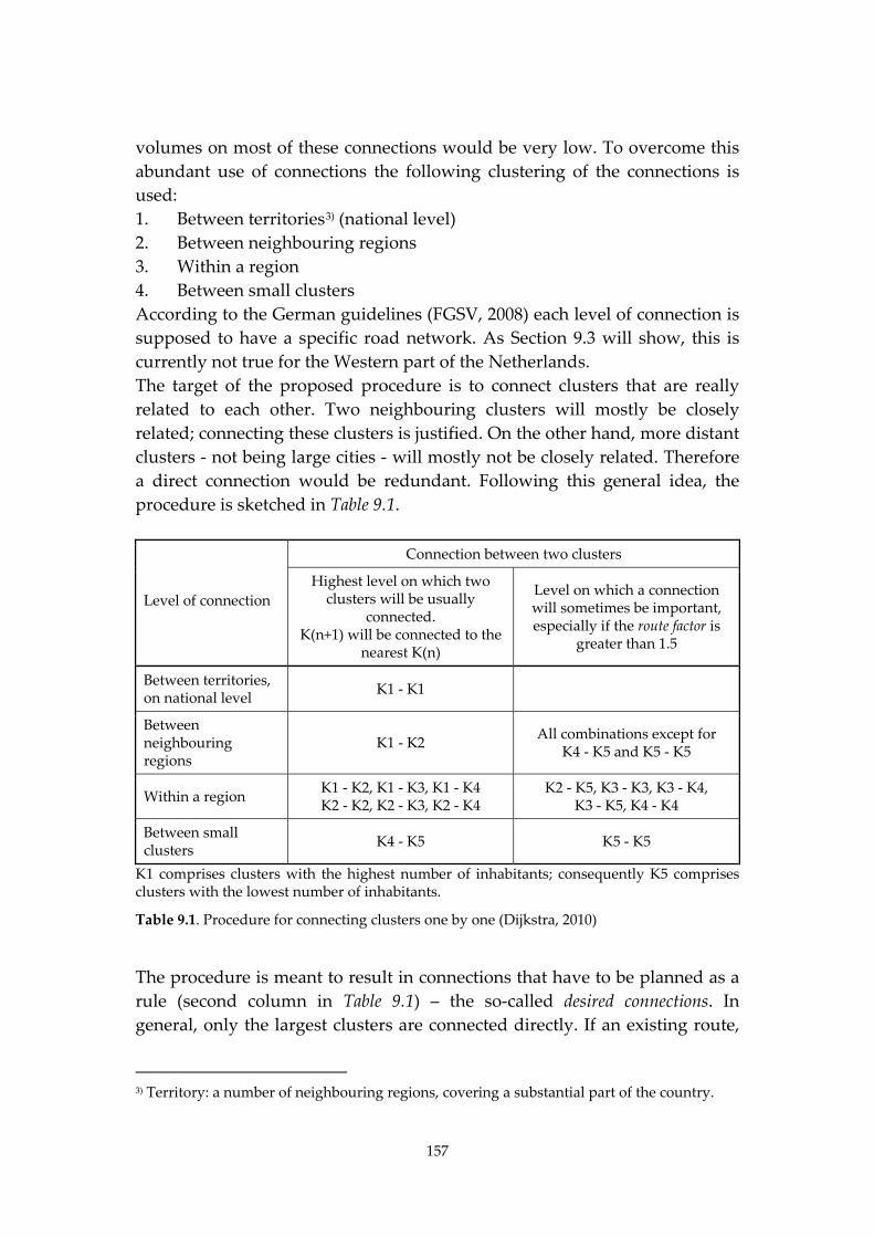
157
volumes on most of these connections would be very low. To overcome this
abundant use of connections the following clustering of the connections is
used:
1. Between territories3) (national level)
2. Between neighbouring regions
3. Within a region
4. Between small clusters
According to the German guidelines (FGSV, 2008) each level of connection is
supposed to have a specific road network. As Section 9.3 will show, this is
currently not true for the Western part of the Netherlands.
The target of the proposed procedure is to connect clusters that are really
related to each other. Two neighbouring clusters will mostly be closely
related; connecting these clusters is justified. On the other hand, more distant
clusters ‐ not being large cities ‐ will mostly not be closely related. Therefore
a direct connection would be redundant. Following this general idea, the
procedure is sketched in Table 9.1.
Connection between two clusters
Level of connection
Highest level on which two clusters will be usually
connected. K(n+1) will be connected to the
nearest K(n)
Level on which a connection will sometimes be important, especially if the route factor is
greater than 1.5
Between territories, on national level
K1 ‐ K1
Between neighbouring regions
K1 ‐ K2 All combinations except for
K4 ‐ K5 and K5 ‐ K5
Within a region K1 ‐ K2, K1 ‐ K3, K1 ‐ K4 K2 ‐ K2, K2 ‐ K3, K2 ‐ K4
K2 ‐ K5, K3 ‐ K3, K3 ‐ K4, K3 ‐ K5, K4 ‐ K4
Between small clusters
K4 ‐ K5 K5 ‐ K5
K1 comprises clusters with the highest number of inhabitants; consequently K5 comprises clusters with the lowest number of inhabitants.
Table 9.1. Procedure for connecting clusters one by one (Dijkstra, 2010)
The procedure is meant to result in connections that have to be planned as a
rule (second column in Table 9.1) – the so‐called desired connections. In
general, only the largest clusters are connected directly. If an existing route,
3) Territory: a number of neighbouring regions, covering a substantial part of the country.
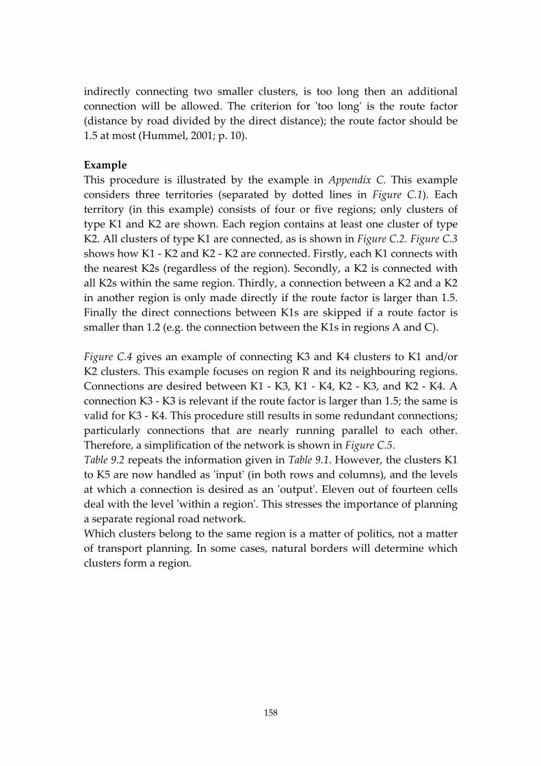
158
indirectly connecting two smaller clusters, is too long then an additional
connection will be allowed. The criterion for ʹtoo longʹ is the route factor
(distance by road divided by the direct distance); the route factor should be
1.5 at most (Hummel, 2001; p. 10).
Example
This procedure is illustrated by the example in Appendix C. This example
considers three territories (separated by dotted lines in Figure C.1). Each
territory (in this example) consists of four or five regions; only clusters of
type K1 and K2 are shown. Each region contains at least one cluster of type
K2. All clusters of type K1 are connected, as is shown in Figure C.2. Figure C.3
shows how K1 ‐ K2 and K2 ‐ K2 are connected. Firstly, each K1 connects with
the nearest K2s (regardless of the region). Secondly, a K2 is connected with
all K2s within the same region. Thirdly, a connection between a K2 and a K2
in another region is only made directly if the route factor is larger than 1.5.
Finally the direct connections between K1s are skipped if a route factor is
smaller than 1.2 (e.g. the connection between the K1s in regions A and C).
Figure C.4 gives an example of connecting K3 and K4 clusters to K1 and/or
K2 clusters. This example focuses on region R and its neighbouring regions.
Connections are desired between K1 ‐ K3, K1 ‐ K4, K2 ‐ K3, and K2 ‐ K4. A
connection K3 ‐ K3 is relevant if the route factor is larger than 1.5; the same is
valid for K3 ‐ K4. This procedure still results in some redundant connections;
particularly connections that are nearly running parallel to each other.
Therefore, a simplification of the network is shown in Figure C.5.
Table 9.2 repeats the information given in Table 9.1. However, the clusters K1
to K5 are now handled as ʹinputʹ (in both rows and columns), and the levels
at which a connection is desired as an ʹoutputʹ. Eleven out of fourteen cells
deal with the level ʹwithin a regionʹ. This stresses the importance of planning
a separate regional road network.
Which clusters belong to the same region is a matter of politics, not a matter
of transport planning. In some cases, natural borders will determine which
clusters form a region.
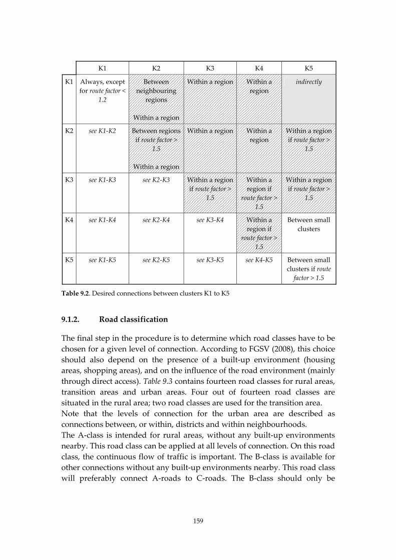
159
K1 K2 K3 K4 K5
K1 Always, except
for route factor <
1.2
Between
neighbouring
regions
Within a region
Within a region Within a
region
indirectly
K2 see K1‐K2 Between regions
if route factor >
1.5
Within a region
Within a region Within a
region
Within a region
if route factor >
1.5
K3 see K1‐K3 see K2‐K3 Within a region
if route factor >
1.5
Within a
region if
route factor >
1.5
Within a region
if route factor >
1.5
K4 see K1‐K4 see K2‐K4 see K3‐K4 Within a
region if
route factor >
1.5
Between small
clusters
K5 see K1‐K5 see K2‐K5 see K3‐K5 see K4‐K5 Between small
clusters if route
factor > 1.5
Table 9.2. Desired connections between clusters K1 to K5
9.1.2. Road classification
The final step in the procedure is to determine which road classes have to be
chosen for a given level of connection. According to FGSV (2008), this choice
should also depend on the presence of a built‐up environment (housing
areas, shopping areas), and on the influence of the road environment (mainly
through direct access). Table 9.3 contains fourteen road classes for rural areas,
transition areas and urban areas. Four out of fourteen road classes are
situated in the rural area; two road classes are used for the transition area.
Note that the levels of connection for the urban area are described as
connections between, or within, districts and within neighbourhoods.
The A‐class is intended for rural areas, without any built‐up environments
nearby. This road class can be applied at all levels of connection. On this road
class, the continuous flow of traffic is important. The B‐class is available for
other connections without any built‐up environments nearby. This road class
will preferably connect A‐roads to C‐roads. The B‐class should only be
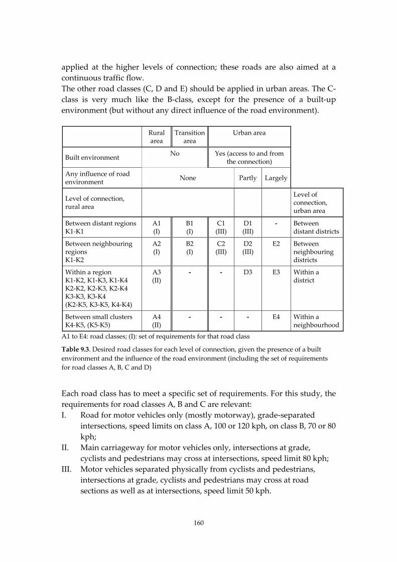
160
applied at the higher levels of connection; these roads are also aimed at a
continuous traffic flow.
The other road classes (C, D and E) should be applied in urban areas. The C‐
class is very much like the B‐class, except for the presence of a built‐up
environment (but without any direct influence of the road environment).
Rural area
Transition area
Urban area
Built environment No
Yes (access to and from the connection)
Any influence of road environment
None Partly Largely
Level of connection, rural area
Level of connection, urban area
Between distant regions K1‐K1
A1 (I)
B1 (I)
C1 (III)
D1 (III)
‐ Between distant districts
Between neighbouring regions K1‐K2
A2 (I)
B2 (I)
C2 (III)
D2 (III)
E2
Between neighbouring districts
Within a region K1‐K2, K1‐K3, K1‐K4 K2‐K2, K2‐K3, K2‐K4 K3‐K3, K3‐K4 (K2‐K5, K3‐K5, K4‐K4)
A3 (II)
‐ ‐ D3
E3
Within a district
Between small clusters K4‐K5, (K5‐K5)
A4 (II)
‐ ‐ ‐ E4
Within a neighbourhood
A1 to E4: road classes; (I): set of requirements for that road class
Table 9.3. Desired road classes for each level of connection, given the presence of a built
environment and the influence of the road environment (including the set of requirements
for road classes A, B, C and D)
Each road class has to meet a specific set of requirements. For this study, the
requirements for road classes A, B and C are relevant:
I. Road for motor vehicles only (mostly motorway), grade‐separated
intersections, speed limits on class A, 100 or 120 kph, on class B, 70 or 80
kph;
II. Main carriageway for motor vehicles only, intersections at grade,
cyclists and pedestrians may cross at intersections, speed limit 80 kph;
III. Motor vehicles separated physically from cyclists and pedestrians,
intersections at grade, cyclists and pedestrians may cross at road
sections as well as at intersections, speed limit 50 kph.
161
Designing a road class, recognising the requirements I to III, is the final step
in the planning and design procedure. This step is not part of this study.
The missing step is how to move from the network of desired connections ‐
described above ‐ to a network that is also inherently safe; this step will be
described in Section 9.2.
9.2. Designing a road network that is inherently safe
Section 9.2 will deal with the design variables for designing an inherently safe
road network. These variables can be positioned on three levels:
Network level
Road class level
Street level
The network level is mainly related to design variables determining the
network structure. Design variables on the road class level are aimed at
satisfying the road class requirements. Finally, the design variables at the
street level focus on arriving at a detailed design of a street (road section and
intersection) that meets the requirements for all types of road users and other
users of the public space (in which the street is situated).
9.2.1. Network level
The network structures that will result in low numbers of crossings4) were
summarized in Section 2.3; these lower numbers should result in more road
safety. Some of these structures also show short distances travelled, which is
also good for road safety. In general, these structures should be chosen
preferentially. However, in existing networks this will be rather difficult to
attain.
The intersection density is a design variable that will determine the locations
of intersections. This location partially depends on requirements and
constraints regarding human factors (minimum sight distance, assumptions
about reaction times, preventing a concentration of situations that need the
driversʹ attention). These implications should be evaluated at the street level.
The mesh of roads, especially of main roads, is a design variable that
influences both the intersection density and the intersection types to be
applied. On the other hand, the mesh partly depends on the distribution of
homes and work places in a given area. However, some freedom in choosing
the mesh remains. Too big a mesh will result in high volumes on the main
4) Crossing with regard to vehicle paths that cross each other.
162
roads and much rat‐run traffic on local roads. Too small a mesh will limit
slow traffic crossing main roads. This last can be prevented by distributing
car traffic more homogeneously over the network.
A second best option is to select a road classification system that will meet
the safety requirements mentioned (crossing, distance travelled) to a large
extent. The road hierarchy is very important for classifying roads. Two main
approaches can be distinguished (Chapter 3):
1. a purely hierarchical approach with a logical sequence of road classes
(Swedish SCAFT);
2. a structure stemming from the existing spatial distribution of homes
and work places in an area (German RAS‐N/RIN).
A strictly hierarchical structure is sometimes of too theoretical a nature to be
applied in practice.
A third target at this level is the minimization of traffic volumes in
residential areas. This target can be reached by road classification or by the
positioning of the area accesses (Section 5.4). Users of access roads (especially
non‐motorized users) will benefit from low volumes on this type of road.
That is why these roads should not be too long, should have a position at the
start/end of the hierarchy, and should mainly be a destination for people
living on that road. Applying these constraints will keep volumes low. When
these constraints are not taken into account, the volumes will depend on the
other design variables (described in this section).
Figure 9.1 shows the targets, the design variables and the ʹbest practicesʹ for
the network level. The best practices are stated in Sections 2.3, 3.3 and 5.4.
9.2.2. Road class level
The road class level applies to design variables ʹwithin a road classʹ. Each
road class is intended to satisfy a set of requirements among others road
safety requirements. These road safety requirements will vary between road
classes. The road classes have the following targets in common:
Minimize the number of serious conflicts (lateral and opposing
conflicts)
Minimize mixing of modes at road sections (the degree of this
minimization depends on the speed limit)
Minimize speed differences
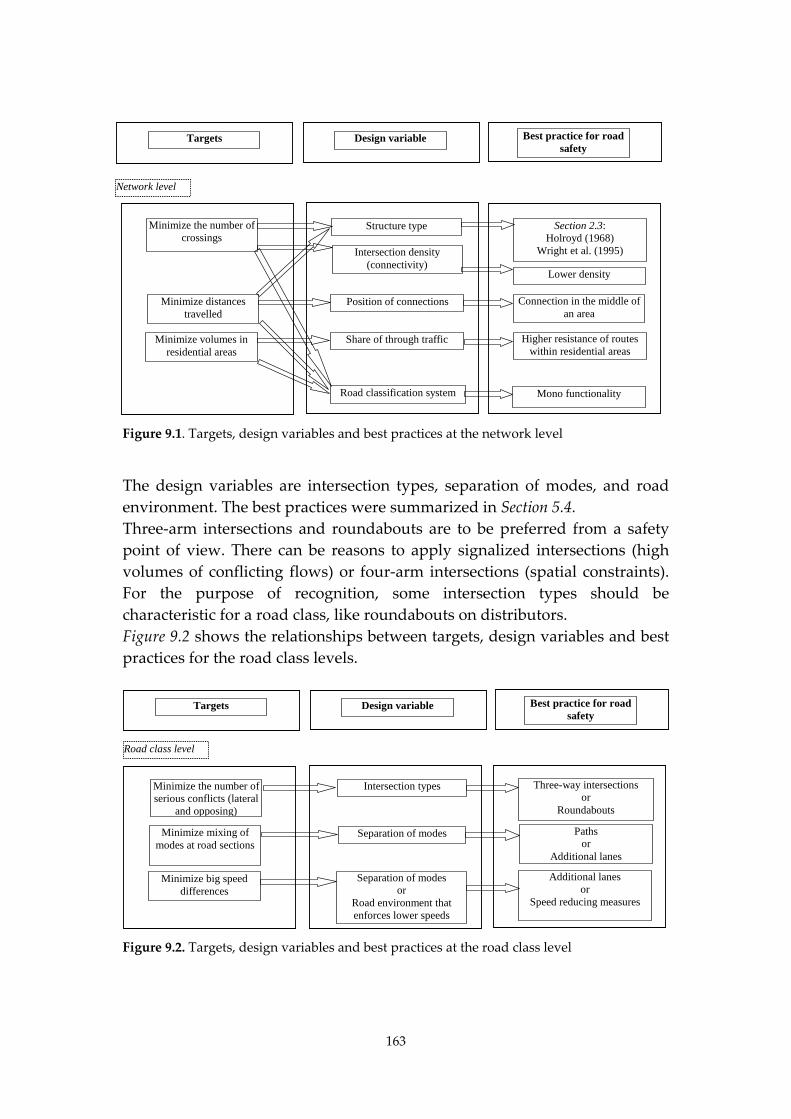
163
Best practice for road safety
Design variable
Minimize the number of crossings
Network level
Minimize distances travelled
Intersection density (connectivity)
Structure type
Minimize volumes in residential areas
Lower density
Section 2.3: Holroyd (1968)
Wright et al. (1995)
Targets
Higher resistance of routes within residential areas
Share of through traffic
Position of connections Connection in the middle of an area
Road classification system Mono functionality
Figure 9.1. Targets, design variables and best practices at the network level
The design variables are intersection types, separation of modes, and road
environment. The best practices were summarized in Section 5.4.
Three‐arm intersections and roundabouts are to be preferred from a safety
point of view. There can be reasons to apply signalized intersections (high
volumes of conflicting flows) or four‐arm intersections (spatial constraints).
For the purpose of recognition, some intersection types should be
characteristic for a road class, like roundabouts on distributors.
Figure 9.2 shows the relationships between targets, design variables and best
practices for the road class levels.
Targets Best practice for road safety
Design variable
Road class level
Minimize the number of serious conflicts (lateral
and opposing)
Minimize mixing of modes at road sections
Minimize big speed differences
Intersection types Three-way intersections or
Roundabouts
Separation of modes
Separation of modes or
Road environment that enforces lower speeds
Paths or
Additional lanes
Additional lanes or
Speed reducing measures
Figure 9.2. Targets, design variables and best practices at the road class level
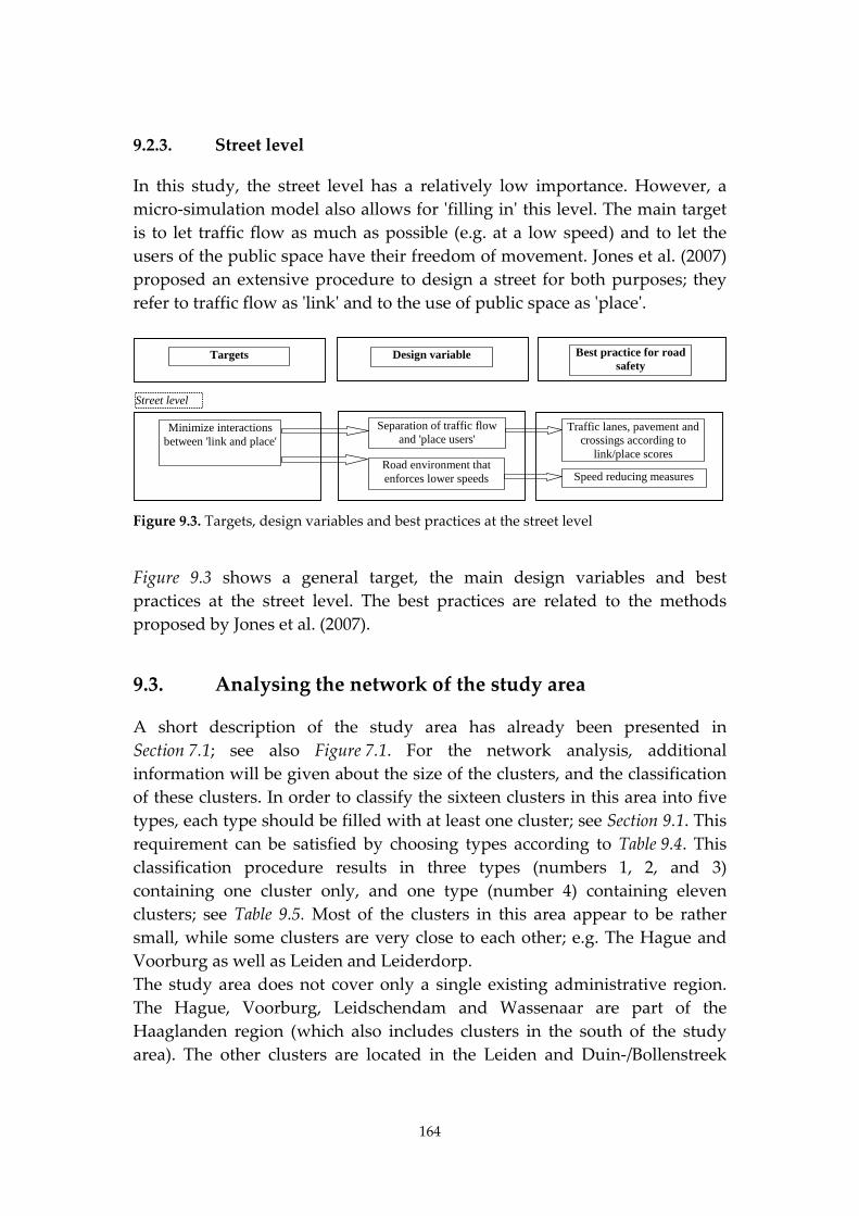
164
9.2.3. Street level
In this study, the street level has a relatively low importance. However, a
micro‐simulation model also allows for ʹfilling inʹ this level. The main target
is to let traffic flow as much as possible (e.g. at a low speed) and to let the
users of the public space have their freedom of movement. Jones et al. (2007)
proposed an extensive procedure to design a street for both purposes; they
refer to traffic flow as ʹlinkʹ and to the use of public space as ʹplaceʹ.
Targets Best practice for road safety
Design variable
Street level
Minimize interactions between 'link and place'
Separation of traffic flow and 'place users'
Traffic lanes, pavement and crossings according to
link/place scores Road environment that enforces lower speeds Speed reducing measures
Figure 9.3. Targets, design variables and best practices at the street level
Figure 9.3 shows a general target, the main design variables and best
practices at the street level. The best practices are related to the methods
proposed by Jones et al. (2007).
9.3. Analysing the network of the study area
A short description of the study area has already been presented in
Section 7.1; see also Figure 7.1. For the network analysis, additional
information will be given about the size of the clusters, and the classification
of these clusters. In order to classify the sixteen clusters in this area into five
types, each type should be filled with at least one cluster; see Section 9.1. This
requirement can be satisfied by choosing types according to Table 9.4. This
classification procedure results in three types (numbers 1, 2, and 3)
containing one cluster only, and one type (number 4) containing eleven
clusters; see Table 9.5. Most of the clusters in this area appear to be rather
small, while some clusters are very close to each other; e.g. The Hague and
Voorburg as well as Leiden and Leiderdorp.
The study area does not cover only a single existing administrative region.
The Hague, Voorburg, Leidschendam and Wassenaar are part of the
Haaglanden region (which also includes clusters in the south of the study
area). The other clusters are located in the Leiden and Duin‐/Bollenstreek
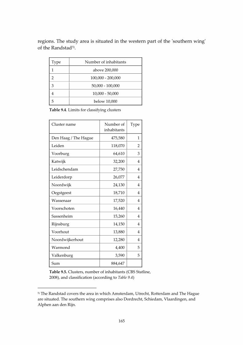
165
regions. The study area is situated in the western part of the ʹsouthern wingʹ
of the Randstad5).
Type Number of inhabitants
1 above 200,000
2 100,000 ‐ 200,000
3 50,000 ‐ 100,000
4 10,000 ‐ 50,000
5 below 10,000
Table 9.4. Limits for classifying clusters
Cluster name Number of
inhabitants
Type
Den Haag / The Hague 475,580 1
Leiden 118,070 2
Voorburg 64,610 3
Katwijk 32,200 4
Leidschendam 27,750 4
Leiderdorp 26,077 4
Noordwijk 24,130 4
Oegstgeest 18,710 4
Wassenaar 17,520 4
Voorschoten 16,440 4
Sassenheim 15,260 4
Rijnsburg 14,150 4
Voorhout 13,880 4
Noordwijkerhout 12,280 4
Warmond 4,400 5
Valkenburg 3,590 5
Sum 884,647
Table 9.5. Clusters, number of inhabitants (CBS Statline,
2008), and classification (according to Table 9.4)
5) The Randstad covers the area in which Amsterdam, Utrecht, Rotterdam and The Hague
are situated. The southern wing comprises also Dordrecht, Schiedam, Vlaardingen, and
Alphen aan den Rijn.
166
The size of an administrative region is not very well defined. The procedure
does not provide a criterion for the size of an area. What are the
consequences of assuming the clusters to be in one or in two regions? Two
options have been considered:
1. all clusters in one region;
2. The Hague, Voorburg, Leidschendam, and Wassenaar in one region,
the other clusters in a second region.
9.3.1. Connecting clusters
In both options, the clusters have been connected according to the procedure
in Section 9.1. In Figure 9.4 (one region) and Figure 9.5 (two regions), all
clusters of type 1 to 4 are connected. A connection begins and ends at the
edge of a large cluster, or in the middle of smaller clusters. The options are
quite different in terms of the number and nature of the connections. Option
1 has many long connections; in Option 2 only the shorter connections are
left.
Regarding the size of both options, Option 2 is closer to the size of the
existing regions in the Netherlands. Both regions in Option 2 were, for many
years, physically separated by an airport. The airport having recently
disappeared, the regions may be more connected in the (near) future.
External clusters
External clusters can have a big influence on the connections in a region.
Relevant external clusters for the study area are Rotterdam (type 1),
Amsterdam (type 1), Zoetermeer (type 2), and Delft (type 3). The simulations
in Chapter 10 will show the influence of external clusters, especially on the
traffic volumes. Traffic entering the study area East of Leiden has to find its
way through the city of Leiden. A new road may be constructed connecting
the A4 and the A44, therefore relieving Leiden of much through traffic. This
new connection will create new routes for a greater area than Leiden itself.
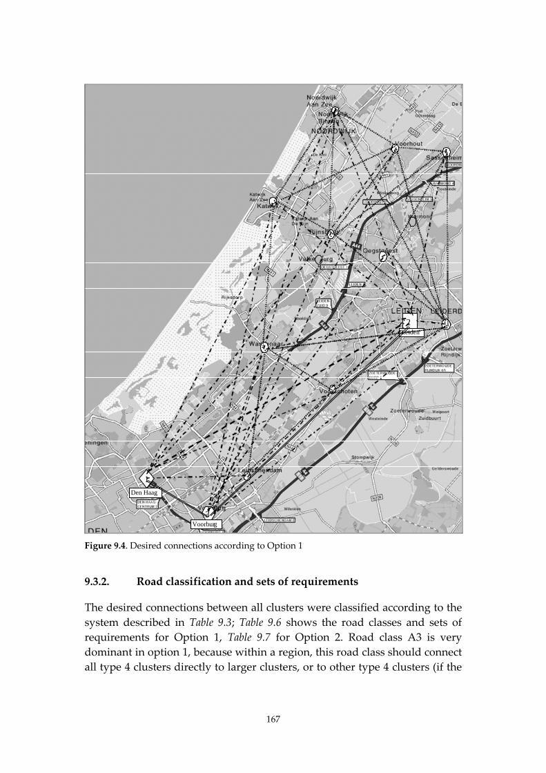
167
Den Haag
Leiden
Voorburg
1
3
2
Figure 9.4. Desired connections according to Option 1
9.3.2. Road classification and sets of requirements
The desired connections between all clusters were classified according to the
system described in Table 9.3; Table 9.6 shows the road classes and sets of
requirements for Option 1, Table 9.7 for Option 2. Road class A3 is very
dominant in option 1, because within a region, this road class should connect
all type 4 clusters directly to larger clusters, or to other type 4 clusters (if the
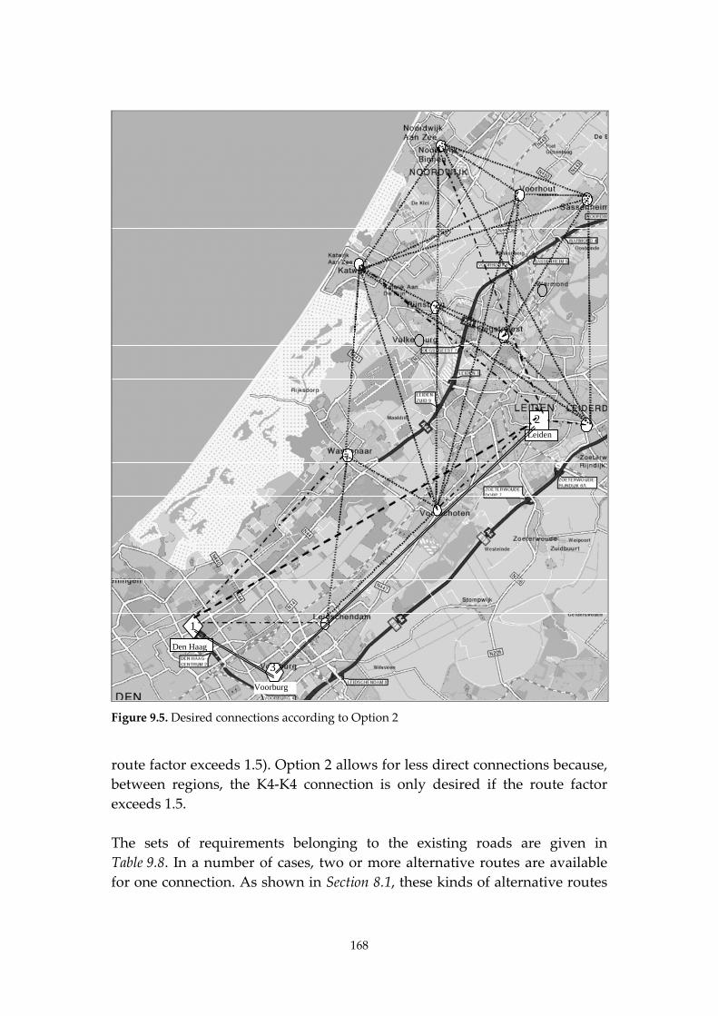
168
Den Haag
Leiden
3
2
1
Voorburg
Figure 9.5. Desired connections according to Option 2
route factor exceeds 1.5). Option 2 allows for less direct connections because,
between regions, the K4‐K4 connection is only desired if the route factor
exceeds 1.5.
The sets of requirements belonging to the existing roads are given in
Table 9.8. In a number of cases, two or more alternative routes are available
for one connection. As shown in Section 8.1, these kinds of alternative routes
169
are actually used for the same O‐D pair. However, the safety of all users of
the O‐D pair should be ensured. Either each of the alternative routes should
meet the requirements of the connection, or road users should be directed
towards the safest alternative(s).
The differences between the desired connections and the existing connections
were checked for both options (one or two regions). The outcome of this
check is that:
1. the desired connection is routed indirectly as well as the existing route
(ʹ‐ʹ sign in Tables 9.9 and 9.10);
2. the desired connection is routed indirectly while the existing route is
routed directly (ʹ+ʹ sign);
3. the requirements for the desired connection are equivalent to the
requirements for the existing connection (ʹ=ʹ sign);
4. the existing connection satisfies requirements better than the desired
connections need to do (ʹ>ʹ sign).
The checks for Option 1 can be viewed in Table 9.9; the checks for Option 2 in
Table 9.10. A first finding is that for many connections, in Option 1 as well as
in Option 2, the existing connections are apparently of a higher quality than
desired. Another result is that, in Option 2, many connections are routed
directly, when they should be routed indirectly. Also, from a point of view of
connectivity, the existing network appears to be of a high quality. On the
other hand, many connections are handled by the same roads. Connections
related to different levels (Table 9.1) are dependent on a small number of
roads. Therefore, these roads must carry a lot of traffic, so the road network
is saturated for many hours a day. Adding more capacity might go hand in
hand with striving for a separate network of connections within a region.
9.3.3. Alternative network designs to be simulated
The ʹtool boxʹ for alternative network designs consists of the ʹintegrated
network designʹ approach (Section 9.1) and several design variables on the
network level as well as on the road class level (Section 9.2). The study area
network can be varied in many ways. This section is considers a few
alternative network designs that will most probably improve both road
safety and traffic flow.
The network analysis showed many connections using the same set of main
roads. An alternative structure should offer (newly built) alternative roads
for relatively short interregional connections. Consequently, the density of
exits and entries onto main roads can be reduced. One drawback of adding
170
more roads is the increasing number of intersections, possibly resulting in
more conflicts and/or different types of conflicts.
Another alternative is to focus on the intersection types, changing four‐way
intersections either into roundabouts or into two three‐way intersections.
These measures should be taken on most of the major intersections of the
network to be sure of finding a result on the network level.
A third alternative adds a completely new main road, while downgrading
the existing main roads from A1 class to A2 class. The best location for a new
road would be between the two existing main roads, next to the railway (The
Hague ‐ Leiden). The new road should only have a few exits and entries.
9.4. Conclusions and recommendations
Chapter 9 describes a method for integrated network design. The method
starts with the definition of clusters in urban areas. Consequently, these
clusters are systematically connected. In the final step, the resulting desired
connections will be compared to the existing connections. An application of
this method to the study area showed that the standards of the existing
connections are higher than the standards of the desired connections.
The application of the method showed one shortcoming. The method does
not give a definition or description of the size of the area to be considered.
The application showed that the optimal size of a region was about one half
of the area studied.
Another issue is the number of alternative routes within one O‐D pair. These
alternative routes are actually used for the same purpose: connecting the O‐D
pair. The standards of these routes can be different. However, the safety of
all users of the O‐D pair should be ensured. Either each of the alternative
routes must meet the requirements of the connection, or road users should be
directed towards the safest alternative(s).
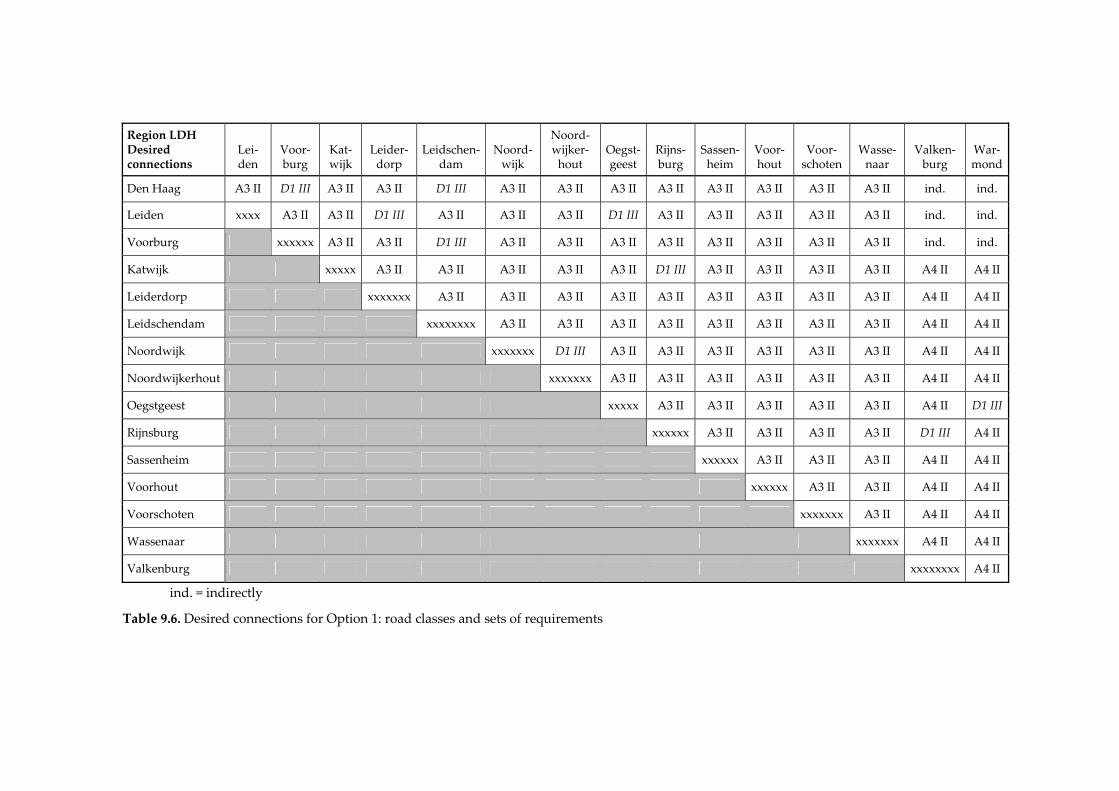
Region LDH Desired connections
Lei‐den
Voor‐burg
Kat‐wijk
Leider‐dorp
Leidschen‐dam
Noord‐wijk
Noord‐wijker‐hout
Oegst‐geest
Rijns‐burg
Sassen‐heim
Voor‐hout
Voor‐schoten
Wasse‐naar
Valken‐burg
War‐mond
Den Haag A3 II D1 III A3 II A3 II D1 III A3 II A3 II A3 II A3 II A3 II A3 II A3 II A3 II ind. ind.
Leiden xxxx A3 II A3 II D1 III A3 II A3 II A3 II D1 III A3 II A3 II A3 II A3 II A3 II ind. ind.
Voorburg xxxxxx A3 II A3 II D1 III A3 II A3 II A3 II A3 II A3 II A3 II A3 II A3 II ind. ind.
Katwijk xxxxx A3 II A3 II A3 II A3 II A3 II D1 III A3 II A3 II A3 II A3 II A4 II A4 II
Leiderdorp xxxxxxx A3 II A3 II A3 II A3 II A3 II A3 II A3 II A3 II A3 II A4 II A4 II
Leidschendam xxxxxxxx A3 II A3 II A3 II A3 II A3 II A3 II A3 II A3 II A4 II A4 II
Noordwijk xxxxxxx D1 III A3 II A3 II A3 II A3 II A3 II A3 II A4 II A4 II
Noordwijkerhout xxxxxxx A3 II A3 II A3 II A3 II A3 II A3 II A4 II A4 II
Oegstgeest xxxxx A3 II A3 II A3 II A3 II A3 II A4 II D1 III
Rijnsburg xxxxxx A3 II A3 II A3 II A3 II D1 III A4 II
Sassenheim xxxxxx A3 II A3 II A3 II A4 II A4 II
Voorhout xxxxxx A3 II A3 II A4 II A4 II
Voorschoten xxxxxxx A3 II A4 II A4 II
Wassenaar xxxxxxx A4 II A4 II
Valkenburg xxxxxxxx A4 II
ind. = indirectly
Table 9.6. Desired connections for Option 1: road classes and sets of requirements
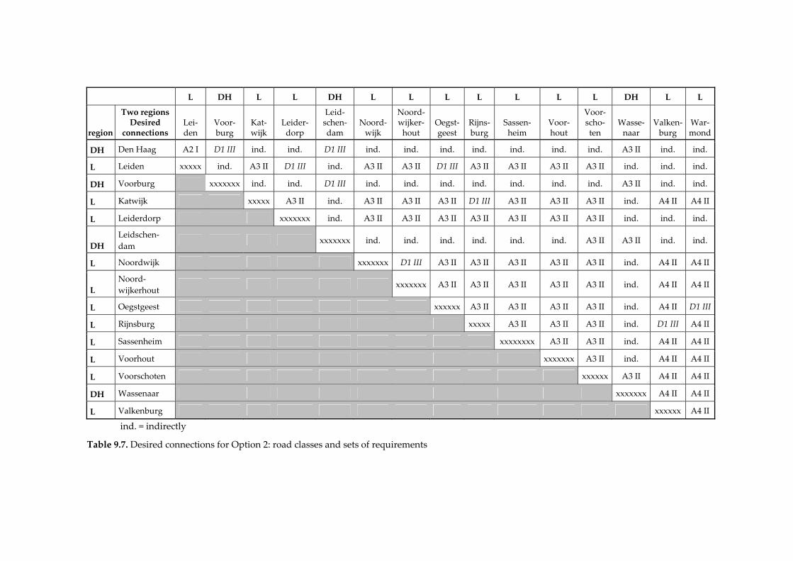
L DH L L DH L L L L L L L DH L L
region
Two regions Desired
connections Lei‐den
Voor‐burg
Kat‐wijk
Leider‐dorp
Leid‐schen‐dam
Noord‐wijk
Noord‐wijker‐hout
Oegst‐geest
Rijns‐burg
Sassen‐heim
Voor‐hout
Voor‐scho‐ten
Wasse‐naar
Valken‐burg
War‐mond
DH Den Haag A2 I D1 III ind. ind. D1 III ind. ind. ind. ind. ind. ind. ind. A3 II ind. ind.
L Leiden xxxxx ind. A3 II D1 III ind. A3 II A3 II D1 III A3 II A3 II A3 II A3 II ind. ind. ind.
DH Voorburg xxxxxxx ind. ind. D1 III ind. ind. ind. ind. ind. ind. ind. A3 II ind. ind.
L Katwijk xxxxx A3 II ind. A3 II A3 II A3 II D1 III A3 II A3 II A3 II ind. A4 II A4 II
L Leiderdorp xxxxxxx ind. A3 II A3 II A3 II A3 II A3 II A3 II A3 II ind. ind. ind.
DH
Leidschen‐
dam xxxxxxx ind. ind. ind. ind. ind. ind. A3 II A3 II ind. ind.
L Noordwijk xxxxxxx D1 III A3 II A3 II A3 II A3 II A3 II ind. A4 II A4 II
L
Noord‐
wijkerhout xxxxxxx A3 II A3 II A3 II A3 II A3 II ind. A4 II A4 II
L Oegstgeest xxxxxx A3 II A3 II A3 II A3 II ind. A4 II D1 III
L Rijnsburg xxxxx A3 II A3 II A3 II ind. D1 III A4 II
L Sassenheim xxxxxxxx A3 II A3 II ind. A4 II A4 II
L Voorhout xxxxxxx A3 II ind. A4 II A4 II
L Voorschoten xxxxxx A3 II A4 II A4 II
DH Wassenaar xxxxxxx A4 II A4 II
L Valkenburg xxxxxx A4 II
ind. = indirectly
Table 9.7. Desired connections for Option 2: road classes and sets of requirements
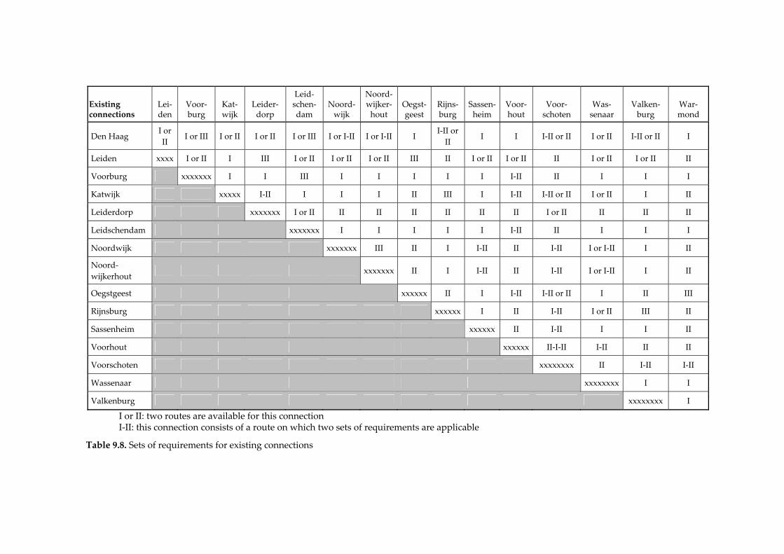
Existing connections
Lei‐den
Voor‐burg
Kat‐wijk
Leider‐dorp
Leid‐schen‐dam
Noord‐wijk
Noord‐wijker‐hout
Oegst‐geest
Rijns‐burg
Sassen‐heim
Voor‐hout
Voor‐schoten
Was‐senaar
Valken‐burg
War‐mond
Den Haag I or
II I or III I or II I or II I or III I or I‐II I or I‐II I
I‐II or
II I I I‐II or II I or II I‐II or II I
Leiden xxxx I or II I III I or II I or II I or II III II I or II I or II II I or II I or II II
Voorburg xxxxxxx I I III I I I I I I‐II II I I I
Katwijk xxxxx I‐II I I I II III I I‐II I‐II or II I or II I II
Leiderdorp xxxxxxx I or II II II II II II II I or II II II II
Leidschendam xxxxxxx I I I I I I‐II II I I I
Noordwijk xxxxxxx III II I I‐II II I‐II I or I‐II I II
Noord‐
wijkerhout xxxxxxx II I I‐II II I‐II I or I‐II I II
Oegstgeest xxxxxx II I I‐II I‐II or II I II III
Rijnsburg xxxxxx I II I‐II I or II III II
Sassenheim xxxxxx II I‐II I I II
Voorhout xxxxxx II‐I‐II I‐II II II
Voorschoten xxxxxxxx II I‐II I‐II
Wassenaar xxxxxxxx I I
Valkenburg xxxxxxxx I
I or II: two routes are available for this connection I‐II: this connection consists of a route on which two sets of requirements are applicable
Table 9.8. Sets of requirements for existing connections
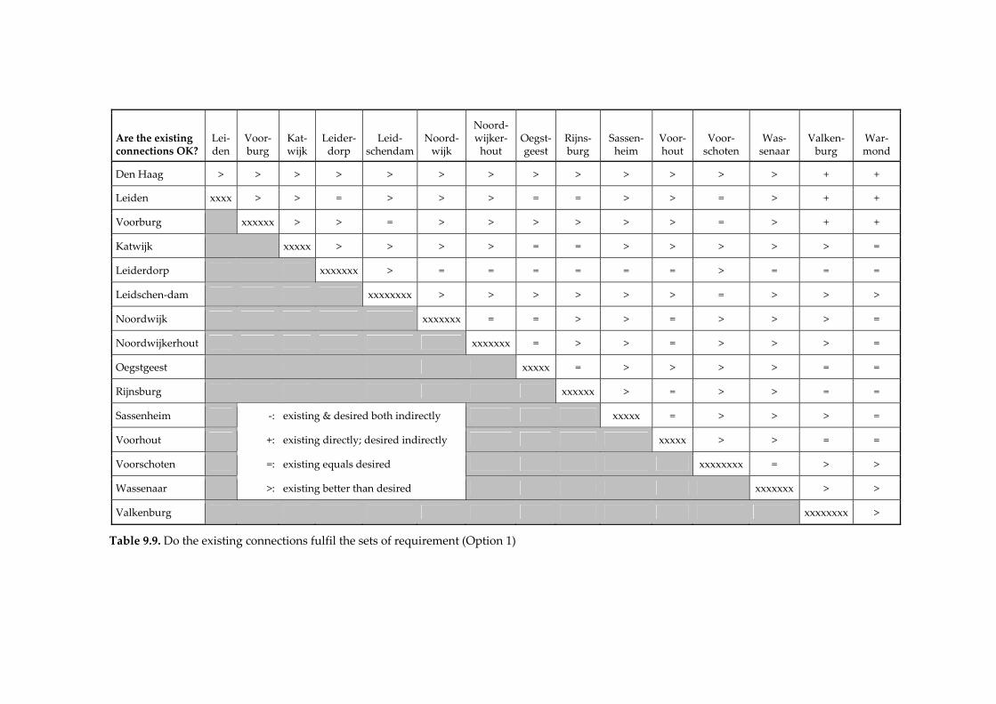
Are the existing connections OK?
Lei‐den
Voor‐burg
Kat‐wijk
Leider‐dorp
Leid‐schendam
Noord‐wijk
Noord‐wijker‐hout
Oegst‐geest
Rijns‐burg
Sassen‐heim
Voor‐hout
Voor‐schoten
Was‐senaar
Valken‐burg
War‐mond
Den Haag > > > > > > > > > > > > > + +
Leiden xxxx > > = > > > = = > > = > + +
Voorburg xxxxxx > > = > > > > > > = > + +
Katwijk xxxxx > > > > = = > > > > > =
Leiderdorp xxxxxxx > = = = = = = > = = =
Leidschen‐dam xxxxxxxx > > > > > > = > > >
Noordwijk xxxxxxx = = > > = > > > =
Noordwijkerhout xxxxxxx = > > = > > > =
Oegstgeest xxxxx = > > > > = =
Rijnsburg xxxxxx > = > > = =
Sassenheim ‐: existing & desired both indirectly xxxxx = > > > =
Voorhout +: existing directly; desired indirectly xxxxx > > = =
Voorschoten =: existing equals desired xxxxxxxx = > >
Wassenaar >: existing better than desired xxxxxxx > >
Valkenburg xxxxxxxx >
Table 9.9. Do the existing connections fulfil the sets of requirement (Option 1)
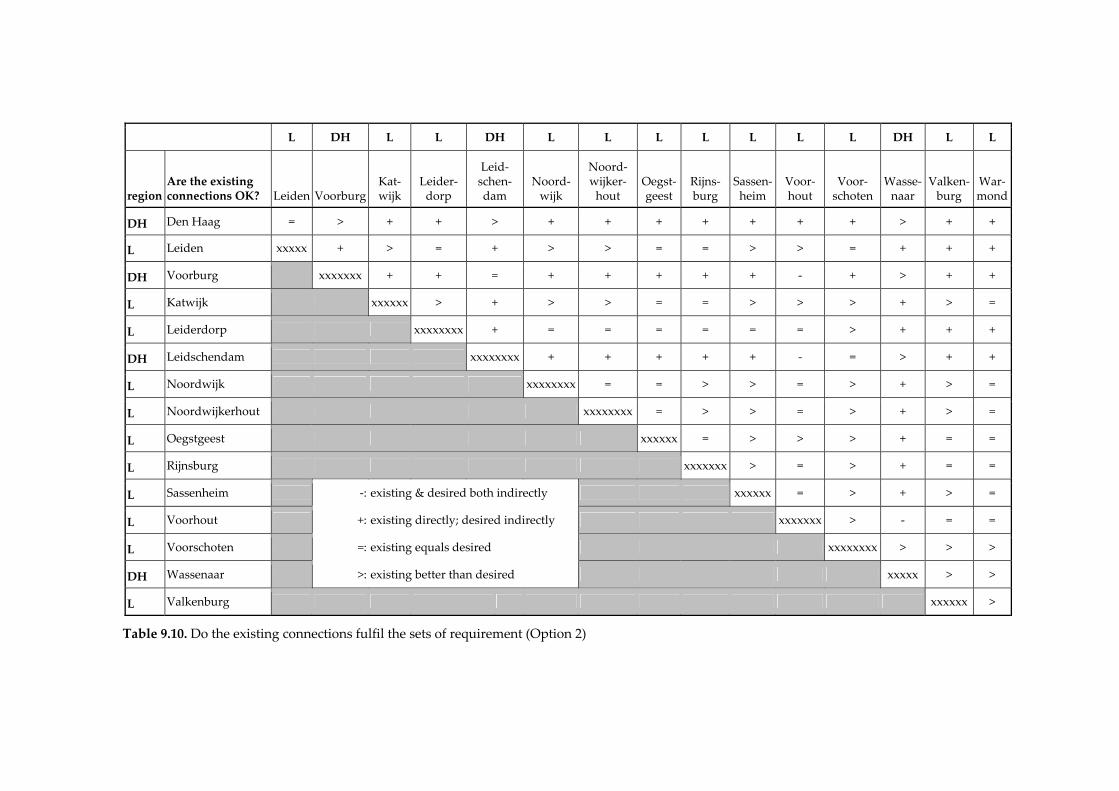
L DH L L DH L L L L L L L DH L L
region Are the existing connections OK? Leiden Voorburg
Kat‐wijk
Leider‐dorp
Leid‐schen‐dam
Noord‐wijk
Noord‐wijker‐hout
Oegst‐geest
Rijns‐burg
Sassen‐heim
Voor‐hout
Voor‐schoten
Wasse‐naar
Valken‐burg
War‐mond
DH Den Haag = > + + > + + + + + + + > + +
L Leiden xxxxx + > = + > > = = > > = + + +
DH Voorburg xxxxxxx + + = + + + + + ‐ + > + +
L Katwijk xxxxxx > + > > = = > > > + > =
L Leiderdorp xxxxxxxx + = = = = = = > + + +
DH Leidschendam xxxxxxxx + + + + + ‐ = > + +
L Noordwijk xxxxxxxx = = > > = > + > =
L Noordwijkerhout xxxxxxxx = > > = > + > =
L Oegstgeest xxxxxx = > > > + = =
L Rijnsburg xxxxxxx > = > + = =
L Sassenheim ‐: existing & desired both indirectly xxxxxx = > + > =
L Voorhout +: existing directly; desired indirectly xxxxxxx > ‐ = =
L Voorschoten =: existing equals desired xxxxxxxx > > >
DH Wassenaar >: existing better than desired xxxxx > >
L Valkenburg xxxxxx >
Table 9.10. Do the existing connections fulfil the sets of requirement (Option 2)
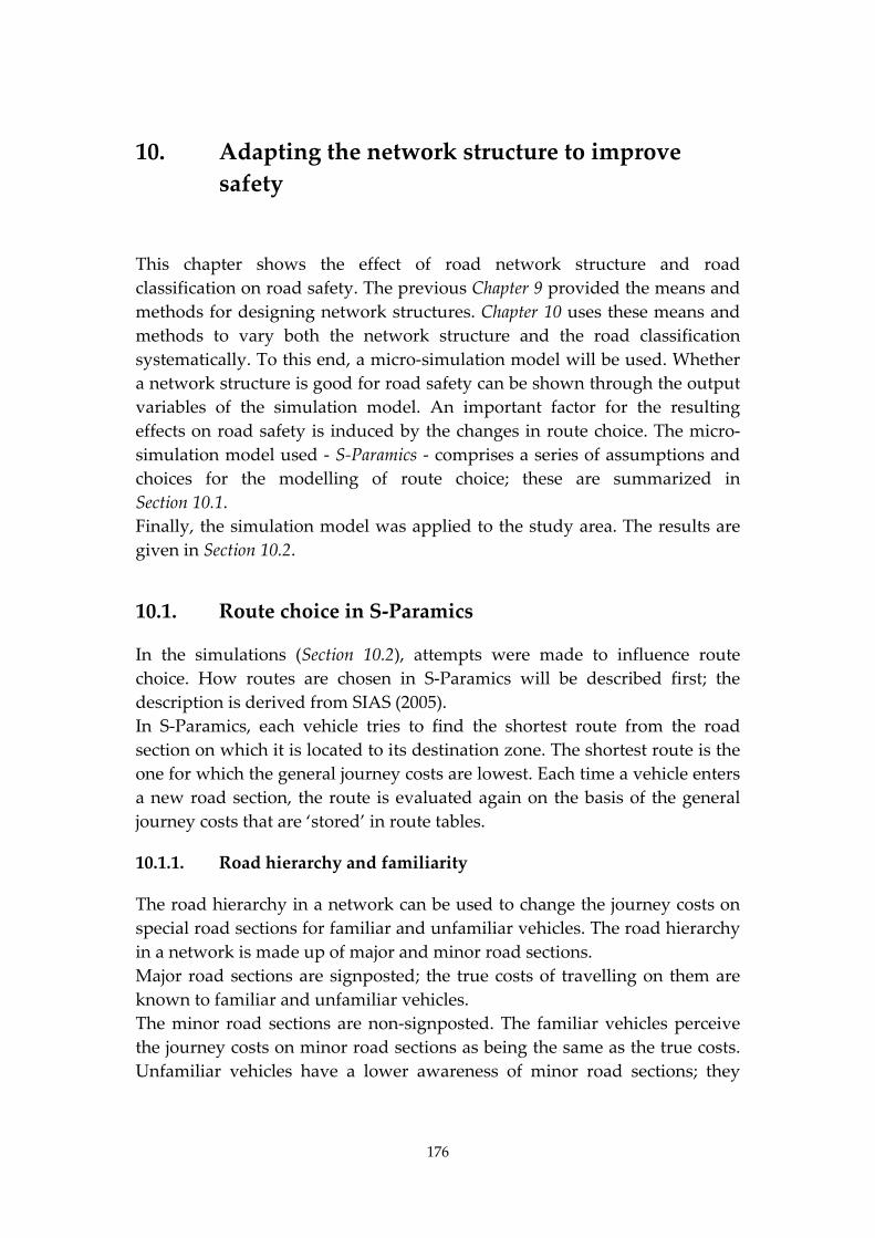
176
10. Adapting the network structure to improve
safety
This chapter shows the effect of road network structure and road
classification on road safety. The previous Chapter 9 provided the means and
methods for designing network structures. Chapter 10 uses these means and
methods to vary both the network structure and the road classification
systematically. To this end, a micro‐simulation model will be used. Whether
a network structure is good for road safety can be shown through the output
variables of the simulation model. An important factor for the resulting
effects on road safety is induced by the changes in route choice. The micro‐
simulation model used ‐ S‐Paramics ‐ comprises a series of assumptions and
choices for the modelling of route choice; these are summarized in
Section 10.1.
Finally, the simulation model was applied to the study area. The results are
given in Section 10.2.
10.1. Route choice in S‐Paramics
In the simulations (Section 10.2), attempts were made to influence route
choice. How routes are chosen in S‐Paramics will be described first; the
description is derived from SIAS (2005).
In S‐Paramics, each vehicle tries to find the shortest route from the road
section on which it is located to its destination zone. The shortest route is the
one for which the general journey costs are lowest. Each time a vehicle enters
a new road section, the route is evaluated again on the basis of the general
journey costs that are ‘stored’ in route tables.
10.1.1. Road hierarchy and familiarity
The road hierarchy in a network can be used to change the journey costs on
special road sections for familiar and unfamiliar vehicles. The road hierarchy
in a network is made up of major and minor road sections.
Major road sections are signposted; the true costs of travelling on them are
known to familiar and unfamiliar vehicles.
The minor road sections are non‐signposted. The familiar vehicles perceive
the journey costs on minor road sections as being the same as the true costs.
Unfamiliar vehicles have a lower awareness of minor road sections; they
177
view the journey costs on these road sections as being twice the true costs.
These ‘penalty costs’ make it less likely that these unfamiliar vehicles will
choose routes along minor road sections and they will therefore tend to stay
on the signposted road sections (i.e. the major road sections).
Familiarity
Familiarity with the road network has a fundamental influence on route
choice in a hierarchical road network. If this directly influences the quantity
of vehicles passing along routes with and without signposting, it is
important to calibrate the level of familiarity properly. The standard
familiarity value for all vehicles is 85%. This means that 85% of the vehicles
make no distinction between the costs of major and minor road sections. The
other 15%, the unfamiliar vehicles, view the costs on minor road sections as
higher and will be more inclined to travel along major road sections.
The level of familiarity can be set separately for each vehicle type. For
example, if a model includes taxis, it would be quite possible to set the
familiarity at 100% because taxi drivers usually know the road network well.
These choices and assumptions in S‐Paramics will actually serve the purpose
of this study. That is because this study would like to offer all the alternative
routes to most of the ʹroad usersʹ (vehicles in this kind of model); the value of
85% is a reasonable assumption. It means that most of the vehicles will view
all available roads as an alternative route. During rush hour, such a high
value can be expected because of the many trips that are made everyday.
This value of 85% was used to calibrate the model described in Section 6.1.
10.1.2. General costs
The general journey costs and the road category can be set for each
individual road section.
General journey costs of a road section
The journey costs of an individual road section can be calculated using the
general cost comparison. This represents a combination of factors that
drivers take into consideration when choosing between various routes. The
most important factors are time and distance. If a toll is charged for using
certain parts of a road, these costs will also be taken into account.
The general journey costs GK of a road section are measured in time, distance
and (if imposed) toll charges. These types of costs are widely used (Ortúzar
& Willumsen; p. 324). GK can be weighted by means of coefficients,
depending on the road category and the familiarity of the road users with the
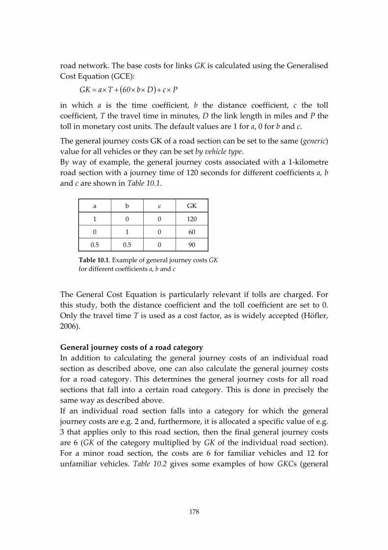
178
road network. The base costs for links GK is calculated using the Generalised
Cost Equation (GCE):
PcDb60TaGK
in which a is the time coefficient, b the distance coefficient, c the toll
coefficient, T the travel time in minutes, D the link length in miles and P the
toll in monetary cost units. The default values are 1 for a, 0 for b and c.
The general journey costs GK of a road section can be set to the same (generic)
value for all vehicles or they can be set by vehicle type.
By way of example, the general journey costs associated with a 1‐kilometre
road section with a journey time of 120 seconds for different coefficients a, b
and c are shown in Table 10.1.
a b c GK
1 0 0 120
0 1 0 60
0.5 0.5 0 90
Table 10.1. Example of general journey costs GK
for different coefficients a, b and c
The General Cost Equation is particularly relevant if tolls are charged. For
this study, both the distance coefficient and the toll coefficient are set to 0.
Only the travel time T is used as a cost factor, as is widely accepted (Höfler,
2006).
General journey costs of a road category
In addition to calculating the general journey costs of an individual road
section as described above, one can also calculate the general journey costs
for a road category. This determines the general journey costs for all road
sections that fall into a certain road category. This is done in precisely the
same way as described above.
If an individual road section falls into a category for which the general
journey costs are e.g. 2 and, furthermore, it is allocated a specific value of e.g.
3 that applies only to this road section, then the final general journey costs
are 6 (GK of the category multiplied by GK of the individual road section).
For a minor road section, the costs are 6 for familiar vehicles and 12 for
unfamiliar vehicles. Table 10.2 gives some examples of how GKCs (general
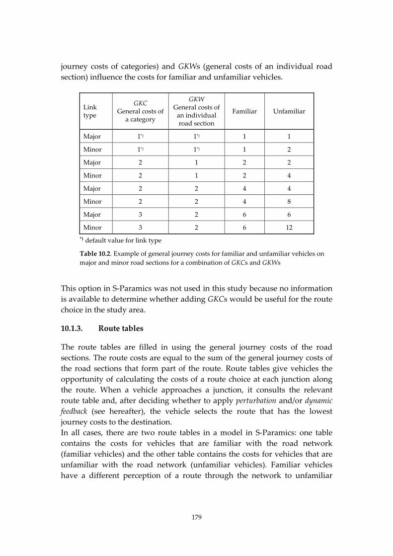
179
journey costs of categories) and GKWs (general costs of an individual road
section) influence the costs for familiar and unfamiliar vehicles.
Link type
GKC General costs of
a category
GKW General costs of an individual road section
Familiar Unfamiliar
Major 1*) 1*) 1 1
Minor 1*) 1*) 1 2
Major 2 1 2 2
Minor 2 1 2 4
Major 2 2 4 4
Minor 2 2 4 8
Major 3 2 6 6
Minor 3 2 6 12
*) default value for link type
Table 10.2. Example of general journey costs for familiar and unfamiliar vehicles on
major and minor road sections for a combination of GKCs and GKWs
This option in S‐Paramics was not used in this study because no information
is available to determine whether adding GKCs would be useful for the route
choice in the study area.
10.1.3. Route tables
The route tables are filled in using the general journey costs of the road
sections. The route costs are equal to the sum of the general journey costs of
the road sections that form part of the route. Route tables give vehicles the
opportunity of calculating the costs of a route choice at each junction along
the route. When a vehicle approaches a junction, it consults the relevant
route table and, after deciding whether to apply perturbation and/or dynamic
feedback (see hereafter), the vehicle selects the route that has the lowest
journey costs to the destination.
In all cases, there are two route tables in a model in S‐Paramics: one table
contains the costs for vehicles that are familiar with the road network
(familiar vehicles) and the other table contains the costs for vehicles that are
unfamiliar with the road network (unfamiliar vehicles). Familiar vehicles
have a different perception of a route through the network to unfamiliar
180
vehicles. This is achieved by making use of a road hierarchy in the network
and by calibrating familiarity.
In addition, a separate route table can be created for each type of vehicle,
thereby producing a set of route tables. Each route table is calculated each
time a simulation is started.
10.1.4. Assignment methods
The following assignment methods are possible in S‐Paramics:
All‐or‐nothing assignment
Stochastic assignment
Dynamic assignment
Stochastic Dynamic assignment
Mayer & Miller (2001; p. 284) also distinguish the equilibrium assignment
method. The stochastic assignment adds a stochastic component to an
equilibrium assignment.
All‐or‐nothing assignment
In a one‐off operation based on an empty network at the start of a simulation,
the all‐or‐nothing assignment determines the general journey costs for all
possible routes associated with an OD relationship. The route with the
lowest general journey costs is seen as the shortest route. All vehicles that
travel from a given origin to a given destination will then make use of this
shortest route.
The all‐or‐nothing assignment was not applied in this study. This type of
assignment does not express the complicated route choices in the networks
to be simulated.
Stochastic assignment
In the stochastic assignment, perturbation is used. Application of perturbation
means that a variance is applied to the general journey costs of a route
whenever vehicles have to choose between routes and do not want to make
use of an all‐or‐nothing assignment.
When a route choice has to be made, a vehicle calculates the general journey
costs GK of each possible route and then takes a random perturbation of these
costs according to the formula below to calculate the new generalised
journey costs GKnew; see for example Willumsen (2008). The route with the
lowest new general journey costs GKnew is chosen.
)100var/GK(GKGKnew
in which onperturbativaronperturbati .
181
The variance, var, can be calculated in one of two ways: by means of the
Percentage algorithm or the Square Root algorithm.
With the Percentage algorithm, the probability is taken into account that the
new general journey costs lie within a margin of P% above or below the
actual costs GK. A perturbation level of 5 (default value) leads to a variance of
5% on the general journey costs GK.
The Square Root algorithm perturbs the general journey costs by making use of
the Burrell technique (Burrell, 1968), based on the following comparison:
C*)500/)P*)5N(((CʹC
in which Cʹ is a random journey time, C is the actual journey time, N is a
random number (from 0 to 10) and P is the perturbation factor (whole
number >0).
For example, if the perturbation factor P equals 100, then the costs will vary by
up to ± C .
The Burrell technique is widely accepted as a reliable way to calculate
journey costs (Ortúzar & Willumsen, 2002), so this study uses the square root
algorithm as part of the stochastic assignment.
Dynamic feedback assignment
In the dynamic feedback assignment, road users who are familiar with the
road network take into consideration the congestion in the network when
calculating the journey costs of a road section and of routes.
Where an all‐or‐nothing assignment calculates the journey costs on the basis
of an empty road network, the dynamic feedback assignment calculates the
journey costs of a road section on the basis of the delay imposed by
congestion in a constantly revised (dynamic) cost calculation.
Road sections that have low journey costs based on calculation for an empty
network, and therefore attract a lot of traffic, will, in the course of time,
produce higher journey costs due to higher concentrations and possibly even
congestion. As a result, alternative routes become more attractive. If the
congestion decreases, the journey costs of these road sections will decline
and become more attractive again.
In the dynamic feedback assignment, the various route tables are constantly
recalculated for each feedback interval.
The frequency of the feedback can be set using the feedback interval. This
means that the journey costs are recalculated every 1, 5 or 10 minutes (for
example) and are used to evaluate the route choice for each individual
vehicle.
182
To avoid excessive variance in the route choice during the simulation period,
a feedback factor is used. This factor takes into account the degree of change in
the journey costs, and it is used to recalculate the choice of route. It is applied
as follows:
previouscurrentnew V*)a1(V*aV
in which a is the feedback coefficient, V the costs of a given movement (from
link to link), Vnew the costs to be used for route choice calculations, Vcurrent the
costs from the current feedback period and Vprevious the costs from the previous
feedback period.
A high feedback factor leads to a higher proportion of delays that are fed
back in the simulation and therefore lead to a greater chance of route
revision. The standard setting for the feedback factor is 0.50.
The dynamic feedback assignment assumes that drivers have knowledge of the
journey costs at a given moment. This can only be true if specific information
is sent periodically to each vehicle. In the simulations described in Section 7.1,
this feedback assignment was not used. However, for finding the theoretical
effects of such a feedback, some of the simulations in Section 10.2 have been
performed by using a dynamic feedback assignment.
Stochastic dynamic assignment
The stochastic dynamic assignment uses both perturbation and feedback and is
therefore the dynamic feedback assignment, together with a varying
perception of the actual general journey costs (perturbation). It is used in
precisely the same way as the stochastic assignment.
This type of assignment was not used in this study because it mixes the
effects of perturbation and feedback. This would interfere with the goal of
the simulations: to separate the effect of perturbation from the effect of
feedback.
10.2. Simulations and analyses
10.2.1. Network structure for simulations
The (main) road network of the study area is shown in Figure 7.1. The
baseline structure for the simulations in this Section 10.2 was derived from
this network. This structure comprises the main road structure of the study
area: five parallel roads are modelled (A4, N44, N447, road through
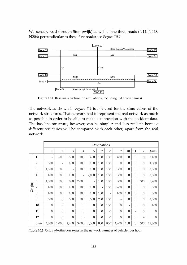
183
Wassenaar, road through Stompwijk) as well as the three roads (N14, N448,
N206) perpendicular to these five roads; see Figure 10.1.
Road through Wassenaar
N44 A44
N14 N448
N447 N447
A4
Road through StompwijkZone 9
Zone 8
Zone 1
Zone 7
Zone 12
Zone 11
Zone 5
Zone 10
Zone 3
Zone 2
Zone 4
Figure 10.1. Baseline structure for simulations (including O‐D zone names)
The network as shown in Figure 7.2 is not used for the simulations of the
network structures. That network had to represent the real network as much
as possible in order to be able to make a connection with the accident data.
The baseline structure, however, can be simpler and less realistic because
different structures will be compared with each other, apart from the real
network.
Destinations
1 2 3 4 5 7 8 9 10 11 12 Sum
1 ‐ 500 500 100 400 100 100 400 0 0 0 2,100
2 500 ‐ 100 100 100 100 100 0 0 0 0 1,000
3 1,500 100 ‐ 100 100 100 100 500 0 0 0 2,500
4 100 100 100 ‐ 2,000 100 100 500 0 0 0 3,000
5 1,000 100 800 2,000 ‐ 100 100 500 0 0 600 5,200
7 100 100 100 100 100 ‐ 100 200 0 0 0 800
8 100 100 100 100 100 100 ‐ 100 100 0 0 800
9 500 0 500 500 500 200 100 ‐ 0 0 0 2,300
10 0 0 0 0 0 0 100 0 ‐ 0 0 100
11 0 0 0 0 0 0 0 0 0 ‐ 0 0
Origins
12 0 0 0 0 0 0 0 0 0 0 ‐ 0
Sum 3,800 1,000 2,200 3,000 3,300 800 800 2,200 100 0 600 17,800
Table 10.3. Origin‐destination zones in the network: number of vehicles per hour
184
Eleven origin‐destination zones were defined to generate traffic in the
network; see Table 10.3 and Figure 10.1. Most of the vehicles are headed
towards The Hague (specifically towards zones 1 and 4). A substantial
number of vehicles are directed from zone 5 towards zones 3 and 12.
The numbers of vehicles do not have any relation to the real O‐D pairs.
Nevertheless, the proportions of the numbers of vehicles are representative
for this area and these roads.
10.2.2. Network variations
Two variations were designed:
1. The baseline structure extended with two connections between A4 and
N44 as well as a minor road next to the A4 (Figure 10.2);
2. The structure according to variation 1 extended with a ʹcentral roadʹ
(Figure 10.3).
The locations and the numbers of the zones were not changed, neither were
the numbers of vehicles between the zones.
Road through Wassenaar
N14 N448
Road bypassing Leiden
N447 N447
A4
Road through Stompwijk
A44N44
Figure 10.2. Variation 1: Road structure, including two connections between A4
and N44
Variation 1 is intended to complement the existing structure by connecting
the two main roads. The A4 is connected indirectly to the N44/A44 to prevent
regional traffic from using the A4.
Variation 2 provides even more capacity to the network in order to relieve
the N44 and N447. However, the connection of this central road to the N14
needed a special design because of the large flow of intersecting vehicles. In
the final design, the intersecting flows are grade separated.
185
Road through Wassenaar
Road next to railway
N448
N14 Road bypassing Leiden
N447 N447
A4
Road through Stompwijk
A44N44
Figure 10.3. Variation 2: Road structure, including both two connections between A4
and N44 and a road next to the railway
10.2.3. Simulation runs
The simulations for the baseline structure and the two variations had the
following characteristics; see also Section 10.1.4:
Ten runs for each structure
Perturbation factor P = 50 for 85% of the vehicles
Variance, var, by means of the square root algorithm
No feedback
Each simulation run covered a period of two hours. During this two‐hour
period, all vehicles departed from their origin zones. To make this happen,
the number of lanes had to be increased at the exits of some busy zones. In
addition, some entries of main roads had to be lengthened. Finally, some
road sections had to be widened (by adding one lane). These alterations
apply to both the baseline structure and the variations. Consequently, the
differences between the three variations are exclusively related to the
availability of the connections.
10.2.4. Volumes on major links by structure
The volumes on the major links of the baseline structure are shown in Figure
10.4. The vehicles can only use a small number of routes. The right‐hand
sides of the N447 and the N448 are used by vehicles driving from zone 5 to
zone 2 and to zone 3. The road through Wassenaar and the left‐hand side of
the N447 are hardly used, mainly due to the perturbation factor and the lack
of feedback.

186
Road through Wassenaar
N44 A44
N14 N448
N447 N447
A4
Road through Stompwijk
V=Volume
5436
5291 6316
58214455
59664442
6008
2647380
2784
384 3125
0
4059
559
0
7535
Figure 10.4. Baseline structure: volumes for major links (for both directions, in number
of vehicles per two hours)
Road through Wassenaar
N14 N448
Road bypassing Leiden
N447 N447
A4
Road through Stompwijk
V=Volume
71%104%
V=154
99% 100%
98% 100%
36%
V=1
V=0
V=442 V=1902
35%4% 38%35%
99%
100%
100%
V=094%
V=104
A44N44
Figure 10.5. Variation 1: volumes for major links (for both directions, in percentage of
baseline structure or in number of vehicles, V, per two hours)
In respect of the use of the N448 and the right‐hand‐side of the N447, the
volumes in Variation 1 are quite different from the baseline structure; (see
Figure 10.5). The road bypassing Leiden as well as a small part of the road
parallel to the A4, take over the traffic from zone 5 to zone 2 and to zone 3.
The new road parallel to the N448 does not have a clear function in this
variation.
In Variation 2, the situation changes even more due to the introduction of the
ʹroad next to the railwayʹ; see Figure 10.6. Many vehicles use that road in
stead of the N44. This new road ends at the road bypassing Leiden; that is
also why that road becomes much busier. The upper part of the road parallel
to the N448 is also used by traffic heading for the N44.
Road through Wassenaar
Road next to railway
N448
N14 Road bypassing Leiden
N447 N447
A4
Road through Stompwijk
V=Volume
60%
78%
98%
66% 71%
102% 100%
V=965
36%
V=1264 191% 134%
35%
5%38%35%
99%
100%
V=1645
V=1653
V=447
V=673
59%
0%88%
V=0
A44N44
Figure 10.6. Variation 2: volumes for major links (for both directions, in percentage of baseline structure or in number of vehicles, V,
per two hours)
188
10.2.5. Conflict numbers, conflict types
Using the approach in Chapter 7, the conflicts (numbers and types) were
derived from the output of the simulations. The output numbers (conflicts or
flows) for each variation are the average of ten simulation runs. The sums of
the numbers of conflicts were calculated for each variation; see Table 10.4.
These conflicts are only related to three‐arm and four‐arm intersections
(called nodes in S‐Paramics). There are rather small differences between the
structures regarding their total numbers (column Sum in Table 10.4). The
variations have a lower number of conflicts than the baseline structure. The
indices in Table 10.5a show that variation 2 has about ten percent fewer
conflicts than the base structure.
Simulation structure RearEnd Lateral Frontal Converging Sum FlowNode
Baseline structure 2,585 8,098 9,203 1,141 21,027 254,181
Variation 1 2,200 9,040 8,064 1,143 20,446 248,807
Variation 2 1,978 8,039 7,531 1,171 18,718 244,559
Table 10.4. All intersections (nodes6)): number of conflicts for each conflict type, total
number of conflicts, and total number of vehicles passing the intersections
(ʹFlownodeʹ)
The conflicts are also segregated into conflict types: rear‐end, lateral, frontal
and converging (Table 10.4). The most severe conflicts are the lateral and
frontal ones; the numbers for these conflicts were taken together in
Table 10.5b. In addition, for these types of conflicts, variation 2 has about ten
percent fewer conflicts than the baseline structure. Variation 1 and the
baseline structure have nearly the same numbers of conflicts.
Simulation structure RearEnd Lateral Frontal Converging Sum FlowNode
Baseline structure 100 100 100 100 100 100
Variation 1 85 112 88 100 97 98
Variation 2 77 99 82 103 89 96
Table 10.5a. Indices for conflict types, total number of conflicts, and total number of
vehicles passing the intersections (baseline structure = 100)
6) S‐Paramics uses the word ʹnodeʹ for all connections of links. Only nodes with at least three
arms have been used for the analyses; these nodes are preferably called ʹintersectionsʹ.
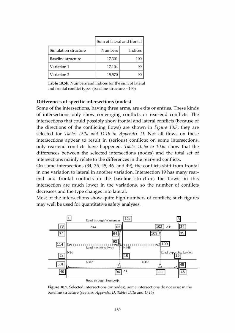
189
Sum of lateral and frontal
Simulation structure Numbers Indices
Baseline structure 17,301 100
Variation 1 17,104 99
Variation 2 15,570 90
Table 10.5b. Numbers and indices for the sum of lateral
and frontal conflict types (baseline structure = 100)
Differences of specific intersections (nodes)
Some of the intersections, having three arms, are exits or entries. These kinds
of intersections only show converging conflicts or rear‐end conflicts. The
intersections that could possibly show frontal and lateral conflicts (because of
the directions of the conflicting flows) are shown in Figure 10.7; they are
selected for Tables D.1a and D.1b in Appendix D. Not all flows on these
intersections appear to result in (serious) conflicts; on some intersections,
only rear‐end conflicts have happened. Tables 10.6a to 10.6c show that the
differences between the selected intersections (nodes) and the total set of
intersections mainly relate to the differences in the rear‐end conflicts.
On some intersections (34, 35, 45, 46, and 49), the conflicts shift from frontal
in one variation to lateral in another variation. Intersection 19 has many rear‐
end and frontal conflicts in the baseline structure; the flows on this
intersection are much lower in the variations, so the number of conflicts
decreases and the type changes into lateral.
Most of the intersections show quite high numbers of conflicts; such figures
may well be used for quantitative safety analyses.
Road through Wassenaar
Road next to railway N448
N14 Road bypassing Leiden
N447 N447
A4
Road through Stompwijk
74
114
12z 8
2z
49
50z
73
15
94 111
34
35
109
10263
10364
19
45
46
93
1
A44N44
Figure 10.7. Selected intersections (or nodes); some intersections do not exist in the
baseline structure (see also Appendix D, Tables D.1a and D.1b)
190
RearEnd Lateral Frontal Converging Sum FlowNode
Selected nodes 1,889 7,955 9,203 1,141 20,189 103,643
All nodes 2,585 8,098 9,203 1,141 21,027 254,181
Percentage sel. nodes 73.1 98.2 100.0 100.0 96.0 40.8
Table 10.6a. Baseline structure ‐ selected nodes versus all nodes: numbers of conflicts
for each conflict type, total number of conflicts, and total numbers of vehicles passing
the intersections
RearEnd Lateral Frontal Converging Sum FlowNode
Selected nodes 1,723 8,868 7,799 1,143 19,533 98,648
All nodes 2,200 9,040 8,064 1,143 20,446 248,807
Percentage sel. nodes 78.3 98.1 96.7 100.0 95.5 39.6
Table 10.6b. Variation 1 ‐ selected nodes versus all nodes: numbers of conflicts for
each conflict type, total number of conflicts, and total numbers of vehicles passing the
intersections
RearEnd Lateral Frontal Converging Sum FlowNode
Selected nodes 1,592 8,039 7,377 1,171 18,179 101,100
All nodes 1,978 8,039 7,531 1,171 18,718 244,559
Percentage sel. nodes 80.5 100.0 98.0 100.0 97.1 41.3
Table 10.6c. Variation 2 ‐ selected nodes versus all nodes: numbers of conflicts for
each conflict type, total number of conflicts, and total numbers of vehicles passing the
intersections
10.2.6. Conflicts related to traffic flow (conflict risk)
The numbers of conflicts, as shown in Table 10.4, are divided by the numbers
of vehicles passing the intersections; see Table 10.7. In this way, the conflict
risk is calculated. The conflict risk values are indexed with relation to the
baseline structure; see Table 10.8. Variation 1 has a much higher risk of lateral
conflicts than the baseline structure. Because of the much lower risks of rear‐
end and frontal conflicts, the average risk (ʹSumʹ in Table 10.7) of Variation 1
equals the average risk of the baseline structure. Variation 2 clearly has a
lower risk than the other two variations. However, Variation 2 also does not
show a better result for lateral conflicts.
191
Simulation structure RearEnd Lateral Frontal Converging Sum
Baseline structure 10.2 31.9 36.2 4.5 82.7
Variation 1 8.8 36.3 32.4 4.6 82.2
Variation 2 8.1 32.9 30.8 4.8 76.5
Table 10.7. Conflict risk for each conflict type, related to the total numbers of vehicles
passing the intersections (divided by 1,000); see absolute numbers in Table 10.4
Simulation structure RearEnd Lateral Frontal Converging Sum
Baseline structure 100 100 100 100 100
Variation 1 87 114 90 102 99
Variation 2 80 103 85 107 93
Table 10.8. Indices regarding conflict risk for each conflict type, related to the total
numbers of vehicles passing the intersections (baseline structure = 100)
10.2.7. Dynamic assignment: feedback in stead of perturbation
The previous simulations used a stochastic assignment (Section 10.2.3), by
using a perturbation factor. The effect of the assignment method on the route
choice was examined by using a dynamic assignment for two structures
(baseline and variation 2). For that purpose, the perturbation in the S‐
Paramics models was switched off, and the feedback was turned on. The
feedback was set to ten minutes, so the routes of all vehicles in the network
were recalculated regularly with an interval of ten minutes. The baseline
structure does not have many alternative routes, so the dynamic assignment
hardly results in any shift to other routes. However, some changes in flows
can be observed. On a few routes, the numbers of passing vehicles increase to
a small extent (between 50 ‐ 300 vehicles), meaning that the flow improves. It
appears that more vehicles have reached their destination within the period
of the simulation run (two hours). The dynamic assessment for variation 2
does not show any change. Apparently, the greater numbers of alternative
routes (compared to the baseline structure) have the same effect on both
assignment methods (perturbation and feedback).
The numbers of conflicts were calculated for the dynamic assignment runs.
The indices for these conflict numbers are given in Tables 10.9a and 10.9b. The
effect of feedback on the numbers of conflicts in variation 2 is very small.
However, the effect on the baseline structure is very large for the rear‐end
192
conflicts. This is probably the effect of the larger numbers of vehicles
finishing their routes, resulting in more conflicts with other vehicles.
Simulation structure RearEnd Lateral FrontalCon‐
vergingSum
Sum of lateral and
frontal
Passingvehicles
Baseline structure 100 100 100 100 100 100 100
Baseline structure, incl. feedback 249 102 105 100 121 104 101
Variation 2 77 99 82 103 89 90 96
Variation 2 incl. feedback 77 100 83 103 90 91 96
Table 10.9a. Indices for conflict types, total number of conflicts, and total number of vehicles
passing the intersections (baseline structure = 100)
The effect is less marked for the lateral and frontal conflicts: 4% more of these
conflicts for the baseline structure, given a small increase (1%) in the number
of passing vehicles (Table 10.9b).
Sum of lateral and frontal Simulation structure
Numbers Indices
Baseline structure 17,301 100
Baseline structure, incl. feedback 17,920 104
Variation 2 15,570 90
Variation 2 incl. feedback 15,679 91
Table 10.9b. Numbers and indices for the sum of lateral and frontal
conflict types (baseline structure = 100)
10.3. Conclusions and recommendations
Three network structures (baseline, variations 1 and 2) were modelled by
way of the S‐Paramics micro‐simulation package. The modelling of the three
network structures (using stochastic assignment) showed rather small
differences in the resulting numbers of conflicts. Both variations resulted in a
lower number of conflicts (3‐ 11%) than the baseline structure. The reduction
of the numbers of ʹseriousʹ conflict types (lateral and frontal) varied from one
to ten percent. Although the number of intersections in variation 2 is higher
than in the baseline structure, the number of serious conflicts decreased. This
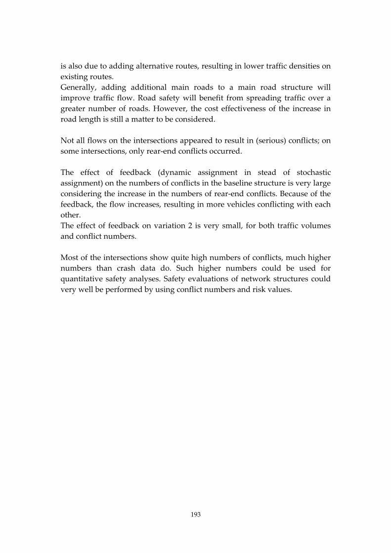
193
is also due to adding alternative routes, resulting in lower traffic densities on
existing routes.
Generally, adding additional main roads to a main road structure will
improve traffic flow. Road safety will benefit from spreading traffic over a
greater number of roads. However, the cost effectiveness of the increase in
road length is still a matter to be considered.
Not all flows on the intersections appeared to result in (serious) conflicts; on
some intersections, only rear‐end conflicts occurred.
The effect of feedback (dynamic assignment in stead of stochastic
assignment) on the numbers of conflicts in the baseline structure is very large
considering the increase in the numbers of rear‐end conflicts. Because of the
feedback, the flow increases, resulting in more vehicles conflicting with each
other.
The effect of feedback on variation 2 is very small, for both traffic volumes
and conflict numbers.
Most of the intersections show quite high numbers of conflicts, much higher
numbers than crash data do. Such higher numbers could be used for
quantitative safety analyses. Safety evaluations of network structures could
very well be performed by using conflict numbers and risk values.
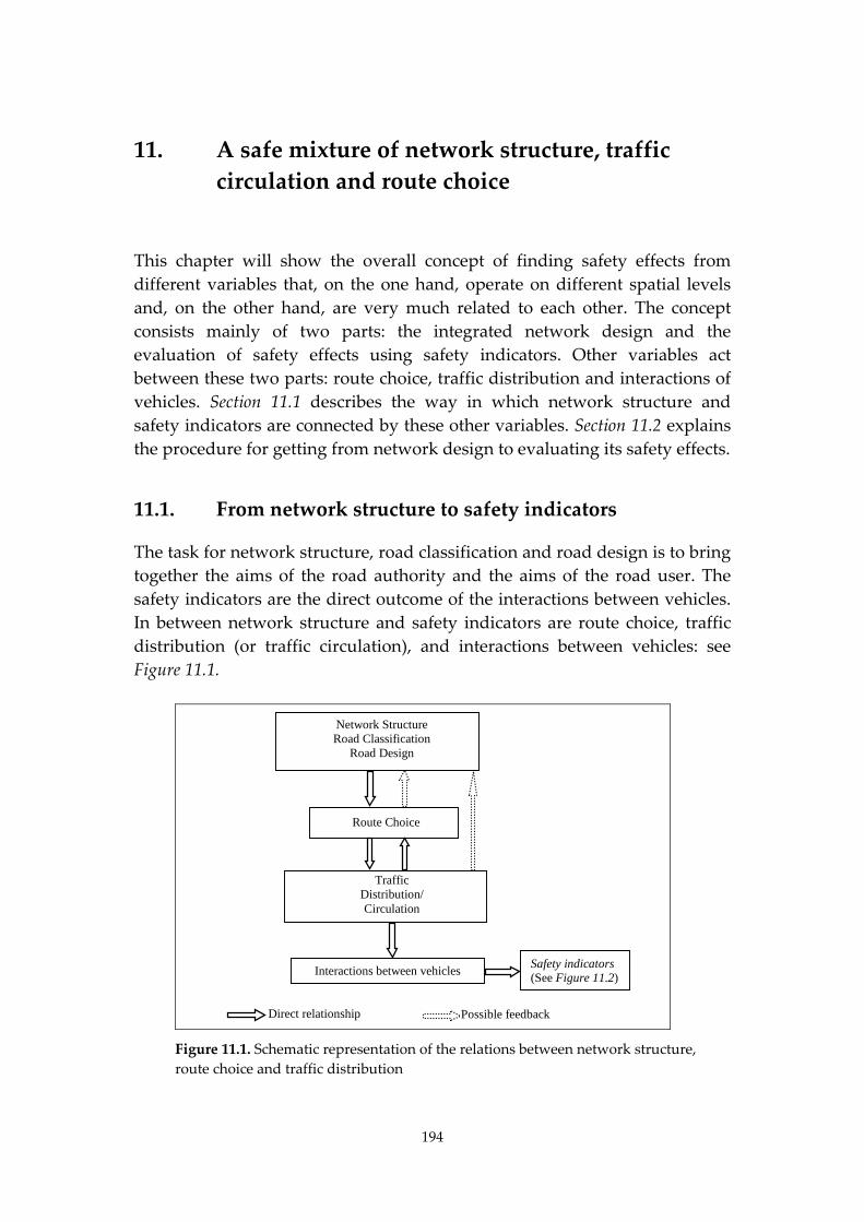
194
11. A safe mixture of network structure, traffic
circulation and route choice
This chapter will show the overall concept of finding safety effects from
different variables that, on the one hand, operate on different spatial levels
and, on the other hand, are very much related to each other. The concept
consists mainly of two parts: the integrated network design and the
evaluation of safety effects using safety indicators. Other variables act
between these two parts: route choice, traffic distribution and interactions of
vehicles. Section 11.1 describes the way in which network structure and
safety indicators are connected by these other variables. Section 11.2 explains
the procedure for getting from network design to evaluating its safety effects.
11.1. From network structure to safety indicators
The task for network structure, road classification and road design is to bring
together the aims of the road authority and the aims of the road user. The
safety indicators are the direct outcome of the interactions between vehicles.
In between network structure and safety indicators are route choice, traffic
distribution (or traffic circulation), and interactions between vehicles: see
Figure 11.1.
Network Structure Road Classification
Road Design
Route Choice
Traffic Distribution/ Circulation
Possible feedback
Interactions between vehicles Safety indicators (See Figure 11.2)
Direct relationship
Figure 11.1. Schematic representation of the relations between network structure,
route choice and traffic distribution
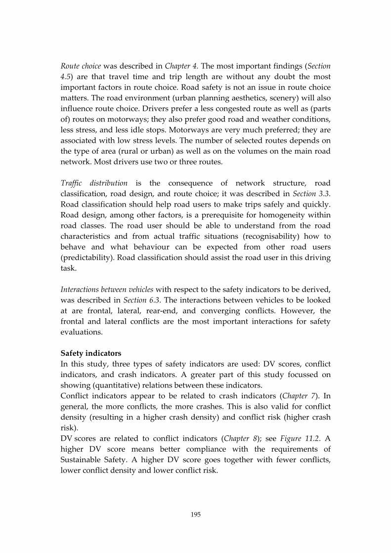
195
Route choice was described in Chapter 4. The most important findings (Section
4.5) are that travel time and trip length are without any doubt the most
important factors in route choice. Road safety is not an issue in route choice
matters. The road environment (urban planning aesthetics, scenery) will also
influence route choice. Drivers prefer a less congested route as well as (parts
of) routes on motorways; they also prefer good road and weather conditions,
less stress, and less idle stops. Motorways are very much preferred; they are
associated with low stress levels. The number of selected routes depends on
the type of area (rural or urban) as well as on the volumes on the main road
network. Most drivers use two or three routes.
Traffic distribution is the consequence of network structure, road
classification, road design, and route choice; it was described in Section 3.3.
Road classification should help road users to make trips safely and quickly.
Road design, among other factors, is a prerequisite for homogeneity within
road classes. The road user should be able to understand from the road
characteristics and from actual traffic situations (recognisability) how to
behave and what behaviour can be expected from other road users
(predictability). Road classification should assist the road user in this driving
task.
Interactions between vehicles with respect to the safety indicators to be derived,
was described in Section 6.3. The interactions between vehicles to be looked
at are frontal, lateral, rear‐end, and converging conflicts. However, the
frontal and lateral conflicts are the most important interactions for safety
evaluations.
Safety indicators
In this study, three types of safety indicators are used: DV scores, conflict
indicators, and crash indicators. A greater part of this study focussed on
showing (quantitative) relations between these indicators.
Conflict indicators appear to be related to crash indicators (Chapter 7). In
general, the more conflicts, the more crashes. This is also valid for conflict
density (resulting in a higher crash density) and conflict risk (higher crash
risk).
DV scores are related to conflict indicators (Chapter 8); see Figure 11.2. A
higher DV score means better compliance with the requirements of
Sustainable Safety. A higher DV score goes together with fewer conflicts,
lower conflict density and lower conflict risk.
196
Figure 11.2. Schematic representation of the relationships between different types
of safety indicators
The conflict indicators are involved in both relations; they are the
intermediate variable between DV scores and crash indicators. So DV scores
are related indirectly to crash indicators (Figure 11.2).
11.2. Network Safety Procedure
Both the application of the integrated network design and the application of
the safety indicators, (referred to above), are part of one procedure or tool
that is meant to find safety effects as a result of changes in the variables
shown in Figure 11.1. This procedure, called Network Safety Procedure
hereafter, consists of eight steps: see also Figure 11.3.
Step 1
The first step of the procedure, designing a network that meets the
requirements of the clustering method, is described by Dijkstra (2010); see
also Section 9.1. The (housing) clusters in a region are connected according to
specific rules, resulting in a number of desired connections. The network
structure is composed of the desired connections. However, some
connections are redundant and may be removed from the final network; see
the example in Section 9.1 (as well as in Appendix C). The connections in the
network structure are already assigned to road classes. However, the final
road classification is also dependant on characteristics of the road
environment (Section 9.1). The road classes should satisfy a set of
requirements as regards the road design.
Step 2
As a consequence, in Step 2, this outcome can be compared with the existing
network. This comparison will possibly show the deficiencies (or surpluses)
Indirect relationship
DV scores
Direct relationship
Conflict indicators
Crash indicators
Safety indicators
197
of the existing network. To that end, the connections in the existing network
should be classified according to the actual road design. This actual road
design is compared to the requirements that were the outcome of Step 1. An
example of such a comparison is described in Section 9.3.
Step 3
Step 3 designs the future network structure, called baseline network
structure. Section 9.2 provides the basic elements for this step. The design
focuses on three levels: network, road class and street level. The targets,
design variables and best practice for road safety are presented for each level
of the road network. The best practice for road safety will help to develop the
design at the levels relevant to the study method chosen. For example, a
micro‐simulation model will require the design of many details. Best practise
will assist in taking this step.
The foregoing three steps are the components of the integrated network design. The
next steps, 4 to 8, are the way to evaluate the safety effects of network structures.
Step 4
Step 4 prepares the calculations for Step 5. There are two options for Step 4.
The first option, building a micro‐simulation model, will make it possible to
calculate conflict indicators. Section 7.1 shows how such a model is built. A
derivative result of this modelling is the output that can be used for
calculating route scores. The second option is the preparation of the data to
be able to calculate route scores without using a simulation model. This
option is used in Section 8.1.
Step 5
In Step 5, the conflict indicators and/or route scores are actually calculated.
The calculation of conflict indicators is automated by using algorithms of the
SAS package (SAS, 2005). The route scores can also be calculated using these
SAS algorithms. In the aforementioned second option the route scores are
calculated by using a spread sheet; see also Section 8.1.
Step 6
Step 6 focuses on designing variations of the baseline structure. These
variations can be the result of evaluating Step 3, or may come from new
insights. This step is applied in Section 9.2.
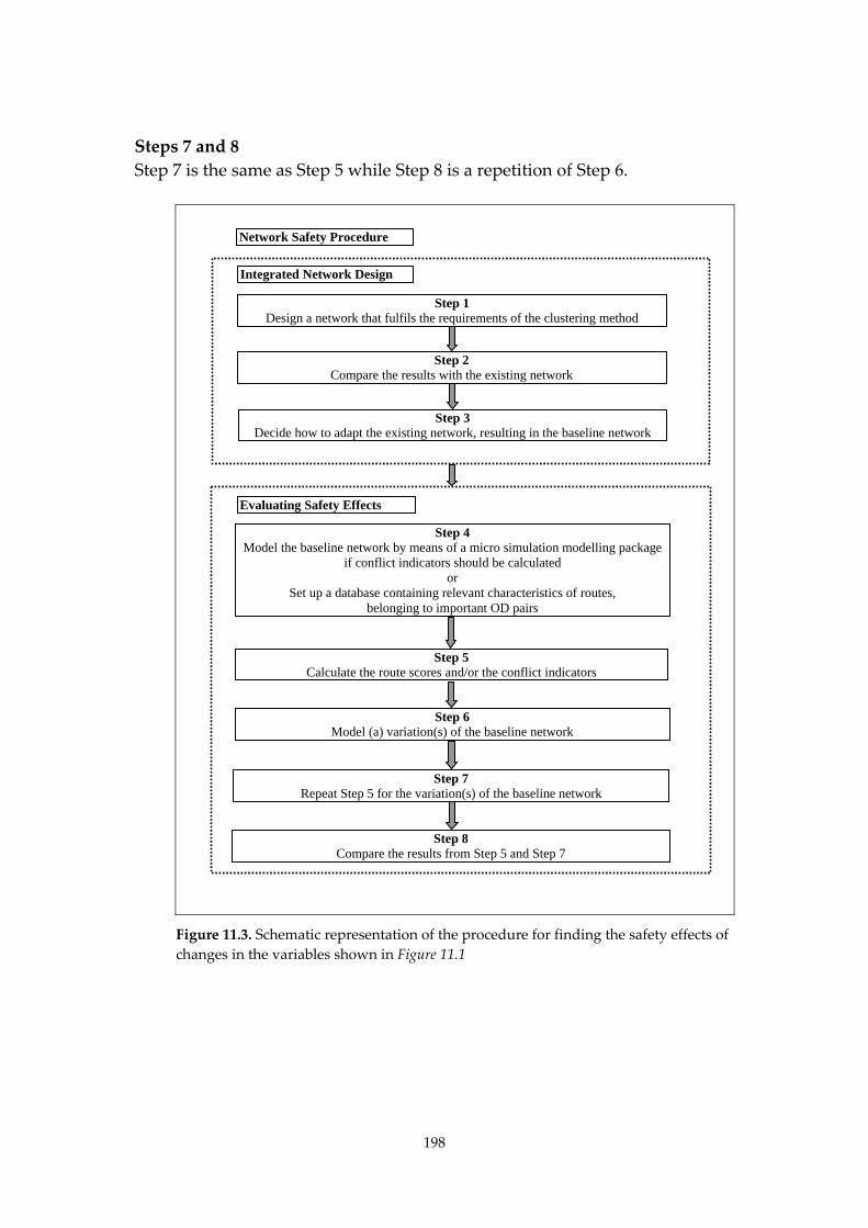
198
Steps 7 and 8
Step 7 is the same as Step 5 while Step 8 is a repetition of Step 6.
Figure 11.3. Schematic representation of the procedure for finding the safety effects of
changes in the variables shown in Figure 11.1
Step 3 Decide how to adapt the existing network, resulting in the baseline network
Step 1 Design a network that fulfils the requirements of the clustering method
Step 2 Compare the results with the existing network
Step 5 Calculate the route scores and/or the conflict indicators
Step 4 Model the baseline network by means of a micro simulation modelling package
if conflict indicators should be calculated or
Set up a database containing relevant characteristics of routes, belonging to important OD pairs
Step 7 Repeat Step 5 for the variation(s) of the baseline network
Step 6 Model (a) variation(s) of the baseline network
Step 8 Compare the results from Step 5 and Step 7
Evaluating Safety Effects
Network Safety Procedure
Integrated Network Design
199
12. Conclusions, discussion, recommendations
This study focused on the effects of changing route choices on road safety.
These changes in route choice are the result of (intended) changes in the
structure of the road network. Alternatively, these changes could be the
consequence of different traffic circulation, e.g. by adapting a traffic signal
system. Thirdly, these changes might be the result of instructions to car
drivers through their navigation systems or their route guidance signs. In
this study, new methods have been developed in order to find the safety
effects of changes in network structure, traffic circulation and route choice.
Combining these methods resulted in a procedure that enables a traffic
planner to find the effects of the mutual influence of these three variables on
road safety.
12.1. Conclusions
12.1.1. Methods and safety indicators
Integrated network design and road classification
In the Netherlands, the methods for arriving at a network structure and a
road classification are not a foregone conclusion. The design principles and
rules of thumb are mostly based on practical experience. The scientific
foundation for this set of principles, requirements and rules is very frail.
A series of requirements was formulated in Sustainable Safety with the
purpose of improving the functioning of the road network safety and
efficiency. The method of ʹintegrated network designʹ was developed to test
whether the road network meets these requirements. Firstly, this method
focuses on the difference between desired and existing connections in the
road network. Different types of clusters (ranging from cities to villages)
should be connected in a structured way. In reality, the road network will
differ from the ideal structure. The next step is to check the difference
between the desired and existing relative position of each connection within
the road network. The final road classification depends on these relative
positions. Road safety is a crucial part of this classification procedure.
Route score ‐ conflict indicator ‐ crash indicator
This study used several safety indicators to find the effects of changes in
route choice. These indicators show a specific aspect of the safety of a route

200
(an unbroken series of road sections and intersections). The route score
describes the general characteristics of a route. A conflict indicator is
calculated by means of a micro‐simulation model. This indicator expresses
the seriousness of conflicts between motor vehicles on and near intersections.
A crash indicator is one of the characteristics of recorded crashes.
Safety as a motive for route choice
Car drivers mention ʹfastest routeʹ and ʹshortest routeʹ as main preferences
for their route choice. The next preference is ʹprior knowledge about a routeʹ.
Car drivers hardly ever take ʹsafety of a routeʹ into consideration when
choosing a route. These results can be found in many studies on route choice.
12.1.2. Relevance for road safety policy and road safety research
Road networks in general
Indicators based on the number of crossing or conflicting vehicles and the
type of these conflicts are relevant if road structures need to be selected for
increased road safety. Literature shows a number of indications of some road
structures having low numbers of crossing vehicles. On the other hand, these
structures can have longer distances travelled, which means more exposure
to risk. In theory, some structures have low numbers of crossings as well as
short distances travelled.
Road safety aspects of network structure and road classification
Countermeasures regarding network structure and road classification appear
to result in crash or casualty reductions ranging from 40 to 80 percent. In
most cases, safety on the surrounding roads hardly worsened, because
additional measures were taken:
The level of through traffic in a square sized residential area (grid
network), is determined by the number and the position of the
connections of the local network to the external network. Connections
in the middle of the sides offer the fastest through routes (no detours).
Connections at the angular points will result in through routes as long
as routes along the surrounding roads. The latter route will be more
attractive because of the higher speed limits on these roads. The more
sides of an area are connected, the shorter the trip length for local traffic
(origin or destination within the area).
Several traffic measures in a residential area (one‐way traffic, street
closures, barring some turning directions on intersections, internal
zoning, and speed reducing provisions) will mostly diminish through
traffic because of the higher resistance of the through routes. Both the

201
local environment and road safety will benefit from these measures.
Traffic volumes on the surrounding roads will mostly increase. The
increasing traffic volume on the surrounding mains roads should be
balanced by the improvements in the areas.
A regional network classified according to Sustainable Safety will most
probably result in a lower number of casualties than a traditional
network. The large numbers of roundabouts in the Sustainable Safety
network will decrease the amount of vehicle hours spent waiting at
signals.
Relation between route score ‐ conflict indicator ‐ crash indicator
A direct relation was found between the number of calculated conflicts and
the number of crashes. The numbers of conflicts are also directly related to
the route score. The number of conflicts is a variable in both relations. That is
why the route score is indirectly related to the number of crashes.
Consequently, the route score is relevant for road safety research.
Route score and conflict indicator
A high value for the route score is related to a lower number of conflicts, to a
lower conflict density, and to a lower conflict risk. In addition, on a selection
of routes containing only the longer routes, a high value for the route score is
related to a lower number of conflicts.
Calculating route scores
The route score consists of a number of safety criteria. Each criterion can be
weighted. The route scores change slightly if the weighting of the criteria is
adapted. These changes are quite small; resulting in hardly any change
between the routes within one OD pair. The weightings are apparently not
necessary to improve the relation between route score and conflict indicators.
Route score and travel time
The routes within one OD pair are compared to each other by means of the
route scores. This comparison shows that the fastest route does not always
have the highest route score. The route with the highest volumes does not
always have the highest route score either.
The number of vehicles on the routes within one OD pair cannot always be
explained by the mean travel time. A shorter travel time is related to fewer
conflicts on a route.
These results depend on the given road network in the study area. Adapting
the structure and characteristics of this network will change these results.
202
Influencing route choice
Prior to a trip, most drivers take note of traffic information, mostly by radio,
television or Internet. This information will largely determine route choice or
departure time. The traffic information en route comes from radio, personal
observation, variable message systems, and, for some drivers, a navigation
system. A substantial proportion of drivers change their route because of this
information.
The expected total effect of navigation systems is: less exposure at the
expense of some loss of attention to the other road users.
12.1.3. Applications
Network structure and conflict indicators
Simulations using different network structures showed small differences in
the number of conflicts. The vehicle flows are spread more evenly over the
network in the network variation with a number of additional connections.
This variation has the lowest number of conflicts as well as a lower conflict
risk. However, the road length is considerably longer.
The effect of feedback (dynamic assignment instead of stochastic assignment)
on the numbers of conflicts in the baseline structure is very large considering
the increasing numbers of rear‐end conflicts. Because of the feedback, the
flow increases, resulting in more vehicles conflicting with each other.
This method, using conflict indicators, produces large numbers of conflicts
on most of the intersections. These numbers are much higher compared to
the numbers of crashes on intersections. Therefore, this method will show
more solid statistical results than crash analyses.
Integrated network design
The application of an integrated network design method to the study area
showed that many connections use roads which have a much higher position
in the road network than desired according to the method. This conclusion
was supported in other (foreign) studies. This finding clearly shows the
structure of the road network in the Netherlands: many main roads
(motorways) facilitating as many connections as possible, disregarding the
distance between the origin and destination of these connections.
The application of the method showed one shortcoming. The method does
not give a definition or description of the size of the area to be considered.
The application showed that the optimal size of a region was about one‐half
of the area studied.
Another issue is the number of alternative routes within one O‐D pair. These
alternative routes are actually used for the same purpose: connecting the O‐D
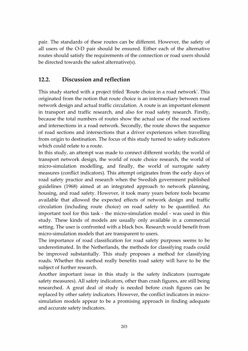
203
pair. The standards of these routes can be different. However, the safety of
all users of the O‐D pair should be ensured. Either each of the alternative
routes should satisfy the requirements of the connection or road users should
be directed towards the safest alternative(s).
12.2. Discussion and reflection
This study started with a project titled ʹRoute choice in a road networkʹ. This
originated from the notion that route choice is an intermediary between road
network design and actual traffic circulation. A route is an important element
in transport and traffic research, and also for road safety research. Firstly,
because the total numbers of routes show the actual use of the road sections
and intersections in a road network. Secondly, the route shows the sequence
of road sections and intersections that a driver experiences when travelling
from origin to destination. The focus of this study turned to safety indicators
which could relate to a route.
In this study, an attempt was made to connect different worlds; the world of
transport network design, the world of route choice research, the world of
micro‐simulation modelling, and finally, the world of surrogate safety
measures (conflict indicators). This attempt originates from the early days of
road safety practice and research when the Swedish government published
guidelines (1968) aimed at an integrated approach to network planning,
housing, and road safety. However, it took many years before tools became
available that allowed the expected effects of network design and traffic
circulation (including route choice) on road safety to be quantified. An
important tool for this task ‐ the micro‐simulation model ‐ was used in this
study. These kinds of models are usually only available in a commercial
setting. The user is confronted with a black box. Research would benefit from
micro‐simulation models that are transparent to users.
The importance of road classification for road safety purposes seems to be
underestimated. In the Netherlands, the methods for classifying roads could
be improved substantially. This study proposes a method for classifying
roads. Whether this method really benefits road safety will have to be the
subject of further research.
Another important issue in this study is the safety indicators (surrogate
safety measures). All safety indicators, other than crash figures, are still being
researched. A great deal of study is needed before crash figures can be
replaced by other safety indicators. However, the conflict indicators in micro‐
simulation models appear to be a promising approach in finding adequate
and accurate safety indicators.
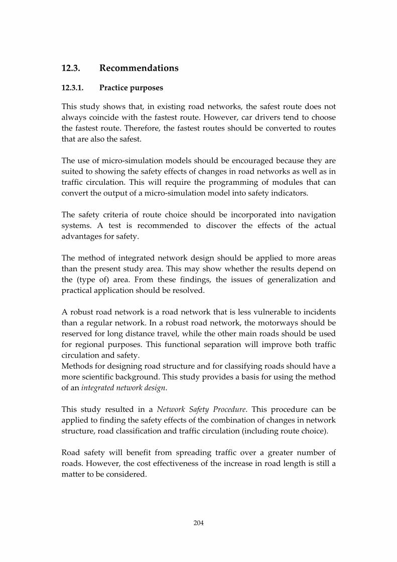
204
12.3. Recommendations
12.3.1. Practice purposes
This study shows that, in existing road networks, the safest route does not
always coincide with the fastest route. However, car drivers tend to choose
the fastest route. Therefore, the fastest routes should be converted to routes
that are also the safest.
The use of micro‐simulation models should be encouraged because they are
suited to showing the safety effects of changes in road networks as well as in
traffic circulation. This will require the programming of modules that can
convert the output of a micro‐simulation model into safety indicators.
The safety criteria of route choice should be incorporated into navigation
systems. A test is recommended to discover the effects of the actual
advantages for safety.
The method of integrated network design should be applied to more areas
than the present study area. This may show whether the results depend on
the (type of) area. From these findings, the issues of generalization and
practical application should be resolved.
A robust road network is a road network that is less vulnerable to incidents
than a regular network. In a robust road network, the motorways should be
reserved for long distance travel, while the other main roads should be used
for regional purposes. This functional separation will improve both traffic
circulation and safety.
Methods for designing road structure and for classifying roads should have a
more scientific background. This study provides a basis for using the method
of an integrated network design.
This study resulted in a Network Safety Procedure. This procedure can be
applied to finding the safety effects of the combination of changes in network
structure, road classification and traffic circulation (including route choice).
Road safety will benefit from spreading traffic over a greater number of
roads. However, the cost effectiveness of the increase in road length is still a
matter to be considered.
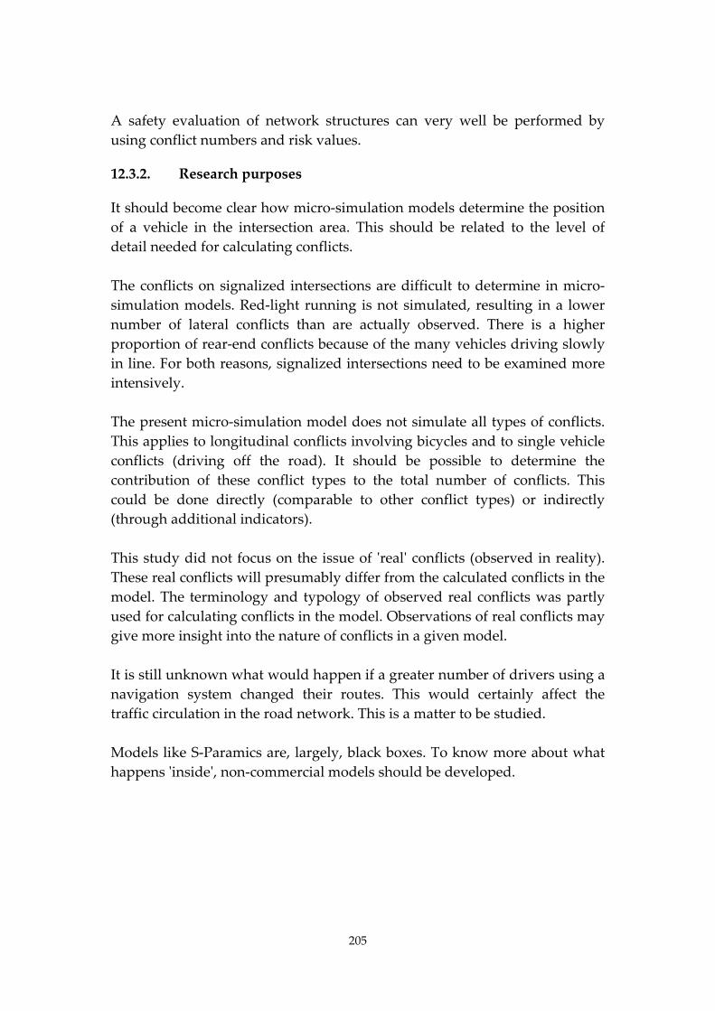
205
A safety evaluation of network structures can very well be performed by
using conflict numbers and risk values.
12.3.2. Research purposes
It should become clear how micro‐simulation models determine the position
of a vehicle in the intersection area. This should be related to the level of
detail needed for calculating conflicts.
The conflicts on signalized intersections are difficult to determine in micro‐
simulation models. Red‐light running is not simulated, resulting in a lower
number of lateral conflicts than are actually observed. There is a higher
proportion of rear‐end conflicts because of the many vehicles driving slowly
in line. For both reasons, signalized intersections need to be examined more
intensively.
The present micro‐simulation model does not simulate all types of conflicts.
This applies to longitudinal conflicts involving bicycles and to single vehicle
conflicts (driving off the road). It should be possible to determine the
contribution of these conflict types to the total number of conflicts. This
could be done directly (comparable to other conflict types) or indirectly
(through additional indicators).
This study did not focus on the issue of ʹrealʹ conflicts (observed in reality).
These real conflicts will presumably differ from the calculated conflicts in the
model. The terminology and typology of observed real conflicts was partly
used for calculating conflicts in the model. Observations of real conflicts may
give more insight into the nature of conflicts in a given model.
It is still unknown what would happen if a greater number of drivers using a
navigation system changed their routes. This would certainly affect the
traffic circulation in the road network. This is a matter to be studied.
Models like S‐Paramics are, largely, black boxes. To know more about what
happens ʹinsideʹ, non‐commercial models should be developed.

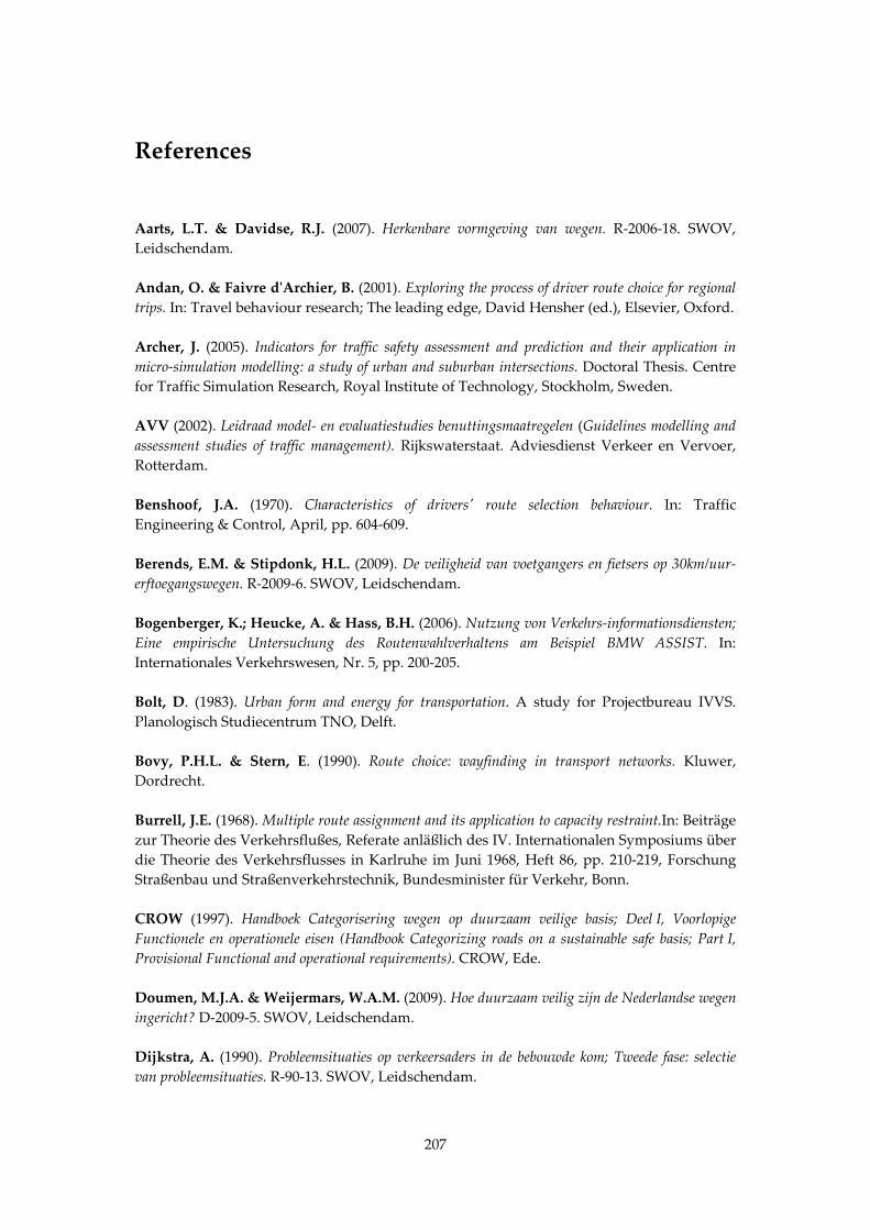
207
References
Aarts, L.T. & Davidse, R.J. (2007). Herkenbare vormgeving van wegen. R‐2006‐18. SWOV,
Leidschendam.
Andan, O. & Faivre dʹArchier, B. (2001). Exploring the process of driver route choice for regional
trips. In: Travel behaviour research; The leading edge, David Hensher (ed.), Elsevier, Oxford.
Archer, J. (2005). Indicators for traffic safety assessment and prediction and their application in
micro‐simulation modelling: a study of urban and suburban intersections. Doctoral Thesis. Centre
for Traffic Simulation Research, Royal Institute of Technology, Stockholm, Sweden.
AVV (2002). Leidraad model‐ en evaluatiestudies benuttingsmaatregelen (Guidelines modelling and
assessment studies of traffic management). Rijkswaterstaat. Adviesdienst Verkeer en Vervoer,
Rotterdam.
Benshoof, J.A. (1970). Characteristics of driversʹ route selection behaviour. In: Traffic
Engineering & Control, April, pp. 604‐609.
Berends, E.M. & Stipdonk, H.L. (2009). De veiligheid van voetgangers en fietsers op 30km/uur‐
erftoegangswegen. R‐2009‐6. SWOV, Leidschendam.
Bogenberger, K.; Heucke, A. & Hass, B.H. (2006). Nutzung von Verkehrs‐informationsdiensten;
Eine empirische Untersuchung des Routenwahlverhaltens am Beispiel BMW ASSIST. In:
Internationales Verkehrswesen, Nr. 5, pp. 200‐205.
Bolt, D. (1983). Urban form and energy for transportation. A study for Projectbureau IVVS.
Planologisch Studiecentrum TNO, Delft.
Bovy, P.H.L. & Stern, E. (1990). Route choice: wayfinding in transport networks. Kluwer,
Dordrecht.
Burrell, J.E. (1968). Multiple route assignment and its application to capacity restraint.In: Beiträge
zur Theorie des Verkehrsflußes, Referate anläßlich des IV. Internationalen Symposiums über
die Theorie des Verkehrsflusses in Karlruhe im Juni 1968, Heft 86, pp. 210‐219, Forschung
Straßenbau und Straßenverkehrstechnik, Bundesminister für Verkehr, Bonn.
CROW (1997). Handboek Categorisering wegen op duurzaam veilige basis; Deel I, Voorlopige
Functionele en operationele eisen (Handbook Categorizing roads on a sustainable safe basis; Part I,
Provisional Functional and operational requirements). CROW, Ede.
Doumen, M.J.A. & Weijermars, W.A.M. (2009). Hoe duurzaam veilig zijn de Nederlandse wegen
ingericht? D‐2009‐5. SWOV, Leidschendam.
Dijkstra, A. (1990). Probleemsituaties op verkeersaders in de bebouwde kom; Tweede fase: selectie
van probleemsituaties. R‐90‐13. SWOV, Leidschendam.
208
Dijkstra, A. (1997). A sustainable safe traffic and transport system: déjà vu in urban planning? In:
Proceedings of the conference Traffic safety on two continents, VTI konferens 9A, Part 3,
September 22‐24, Lisbon.
Dijkstra, A. (2003). Kwaliteitsaspecten van duurzaam‐veilige weginfrastructuur (Quality aspects of
a sustainably safe road infrastructure). Report R‐2003‐10. SWOV, Leidschendam.
Dijkstra, A. (2010). Welke aanknopingspunten bieden netwerkopbouw en wegcategorisering om de
verkeersveiligheid te vergroten? Eisen aan een duurzaam‐veilig wegennet. R‐2010‐3. SWOV,
Leidschendam.
Dijkstra, A.; Drolenga, J. & Maarseveen, M.F.A.M. van (2007). A method for assessing the
safety of routes in a road network. In: Transportation Research Record, No. 2019, pp. 82‐90,
Transportation Research Board, Washington D.C.
Dijkstra, A.; Marchesini, P.; Bijleveld, F.; Kars, V.; Drolenga, H. & Maarseveen, M. van
(2010). Do calculated conflicts in microsimulation model predict number of crashes? In:
Transportation Research Record, No. 2147, pp. 105‐112, Transportation Research Board,
Washington D.C.
Dijkstra, A. & Hummel, T. (2004). Veiligheidsaspecten van het concept ʹBypasses voor
bereikbaarheidʹ. R‐2004‐6. SWOV, Leidschendam.
Dijkstra, A. & Pol, W.H.M. van de (1991). Effecten op leefbaarheid: aspect verkeersveiligheid;
Studie effecten openstelling ringweg Amsterdam. Rijkswaterstaat. Dienst Verkeerskunde,
Rotterdam.
Drolenga, J. (2005). Het ontwerp van een verkeersveiligheidsindicator van routes (designing a safety
indicator for routes). MSc thesis. Twente University, Enschede.
DVS (2008). Analyse nadelige effecten navigatiesystemen op routekeuze. Gebruik en misbruik van
wegen; deel 2. Rijkswaterstaat, Dienst Verkeer en Scheepvaart, Delft.
Engel, U. & Thomsen, L.K. (1983). Trafiksanering på Østerbro; Sammenfatning. Rådet for
Trafiksikkerhedsforskning, Copenhagen.
Erke, H. & Zimolong, B. (1978). Verkehrskonflikte im Innerortsbereich: eine Untersuchung zur
Verkehrskonflikttechnik. Unfall‐ und Sicherheitsforschung Straßenverkehr. Heft 15. Bundes‐
anstalt für Straßenwesen, Köln.
Erke, H. & Gstalter, H. (1985). Verkehrskonflikttechnik: Handbuch für die Durchführung und
Auswertung von Erhebungen. Unfall‐ und Sicherheitsforschung Straßenverkehr. Heft 52.
Bundesanstalt für Straßenwesen, Köln.
Ewing, R. (2000). Sketch planning a street network. In: Transportation Research Record 1722,
pp. 75‐79. Transportation Research Board, Washington D.C.
209
FGSV (1988). Richtlinien für die Anlage von Straβen RAS. Teil: Leitfaden für die funktionelle
Gliederung des Straβennetzes RAS‐N. Forschungsgesellschaft für Straβen‐ und Verkehrswesen
FGSV, Köln.
FGSV (2008). Richtlinien für integrierte Netzgestaltung RIN. Forschungsgesellschaft für
Straβen‐ und Verkehrswesen FGSV, Köln.
FHWA (2000). Prediction of the expected safety performance of rural two‐lane highways. FHWA‐
RD‐99‐207, McLean, Virginia, USA.
FHWA (2003). Surrogate safety measures from traffic simulation models. Report FHWA‐RD‐03‐
050. Federal Highway Administration, McLean, Virginia, USA.
FHWA (2005). Validation of accident models for intersections. FHWA‐RD‐03‐037, McLean,
Virginia, USA.
Gadd, M.L. (1997). Road network planning ‐ towards a comprehensive approach. In: IPENZ
Transactions, Volume 24, No. 1/CE.
Gerlach, J. (2007). Von den RAS‐N zu den RIN ‐ Neue Regeln für die Netzgestaltung und ‐
bewertung. In: Straßenverkehrstechnik, Nr. 6, pp. 281 ‐ 288.
Goldenbeld, Ch.; Drolenga, J. & Smits, A. (2006). Routekeuze van automobilisten; Resultaten
van een vragenlijstonderzoek. R‐2006‐33. SWOV, Leidschendam.
Goudappel, H.M. & Perlot, J.A. (1965). Verkeer en stad. In: Stedebouwkundige studies 4.
Vuga, s.l.
Groenendijk, J.M.; Verroen, E.J. & Zwart, J.C. van der (2004). Regionale bereikbaarheid in de
nota Mobiliteit. In: Innovatie: van inspiratie naar realisatie?, Bundeling van bijdragen aan
Colloquium Vervoersplanologisch Speurwerk, 24‐25 november, CVS, Delft.
Hadayeghi, A.; Shalaby, A.S. & Persaud, B.N. (2003). Macrolevel accident prediction models for
evaluating safety of urban transportation systems. In: Transportation Research Record 1840.
pp. 87‐95. Transportation Research Board, Washington, D.C.
Hadayeghi, A.; Shalaby, A.S. & Persaud, B.N. (2007). Safety prediction models; Proactive tool
for safety evaluation in urban transportation planning applications. In: Transportation Research
Record 2019. pp. 225‐236. Transportation Research Board, Washington, D.C.
Hidas, P. (2005). A functional evaluation of the AIMSUN, PARAMICS and VISSIM
microsimulation models. In: Road & Transport Research, Volume 14, Nr. 4, pp. 45 ‐ 59.
Hidber, C.F. (2001). Städtebau und Verkehr.; Thesen ‐ Modelle ‐ Analysen. In: Strasse und
Verkehr, Nr. 2, pp. 37‐ 45.
Höfler, F. (2006). Verkehrwesen‐Praxis; Band 2: Verkehrstechnik. Bauwerk Verlag, Berlin.

210
Holroyd, E.M. (1966). Theoretical average journey lenghts in circular towns with various routeing
systems. Report 43. Transport and Road Research Laboratory, Crowthorne.
Holroyd, E.M. (1968). Routing traffic in a square town to minimize route‐crossings, In: Beiträge
zur Theorie des Verkehrsflußes, Referate anläßlich des IV. Internationalen Symposiums über
die Theorie des Verkehrsflusses in Karlruhe im Juni 1968, Heft 86, pp. 175‐183, Forschung
Straßenbau und Straßenverkehrstechnik, Bundesminister für Verkehr, Bonn.
Holroyd, E.M. & Miller, A.J. (1966). Route crossings in urban areas. In: A.R.R.B. Proceedings,
Volume 3, Part I, pp. 394‐419.
Horst, A.R.A. van der (1990). A time‐based analysis of road user behaviour in normal and critical
encounters. PhD thesis. Delft University of Technology. Institute for Perception IZF TNO,
Soesterberg.
Hummel, T. (2001b). Toetsing van het gehalte duurzame veiligheid met Safer Transportation
Network Planning. D‐2001‐16. SWOV, Leidschendam.
Hydén, C. (1987). The development of a method for traffic safety evaluation. Lund University,
Lund.
IHT (1996). Guidelines for road safety audit. The Institution of Highways & Transportation
IHT, London.
Immers, L.H.; Wilmink, I.R. & Stada, J.E. (2001). Bypasses voor bereikbaarheid (Bypasses for
accessibility). TNO‐report INRO‐VV/2001‐28. TNO Inro. Afdeling Verkeer en Vervoer, Delft.
Infopunt DV (1999). Duurzaam‐veilige inrichting van wegen buiten de bebouwde kom; Een
gedachtevorming. Infopunt Duurzaam Veilig Verkeer, Ede.
Infopunt DV (2000). Duurzaam‐veilige inrichting van wegen binnen de bebouwde kom; Een
gedachtevorming. Infopunt Duurzaam Veilig Verkeer, Ede.
Jansen, G.R.M. & Bovy, P.H.L. (1974a). An analysis of the size of network models.
Memorandum No. RAV/2/74.3. Institute for Town Planning Research. Delft University of
Technology, Delft.
Jansen, G.R.M. & Bovy, P.H.L. (1974b). Road network size related to city size: empirical findings.
Memorandum No. RAV/2/74.4. Institute for Town Planning Research. Delft University of
Technology, Delft.
Jansen, G.R.M. & Bovy, P.H.L. (1975). Urban road network size: some Dutch findings.
Memorandum No. RAV/2/75.2. Institute for Town Planning Research. Delft University of
Technology, Delft.
Jansen, G.R.M. & Vuren, T. van (1985). De externe vervoersrelaties van de vier grote steden in
Nederland: een empirische studie. Instituut voor Stedebouwkundig Onderzoek, Technische
Hogeschool Delft.
211
Janssen, S.T.M.C. (1974). Verkeersveiligheid als criterium voor het wegontwerp. In: Wegontwerp
en verlichting tegen de achtergrond van de verkeersveiligheid; Preadviezen congresdag
1974, Vereniging Het Nederlandsche Wegencongres, , Den Haag, pp. 13‐40.
Janssen, S.T.M.C. (1988). De verkeersonveiligheid van wegtypen in 1986 en 2010. (The safety of
road types in 1986 and 2010). R‐88‐3. SWOV, Leidschendam.
Janssen, S.T.M.C. (1991a). De categorie‐indeling van wegen binnen de bebouwde kom; Een neerslag
van overwegingen binnen de CROW‐groep. R‐91‐44. SWOV Institute for Road Safety Research,
Leidschendam.
Janssen, S.T.M.C. (1991b). Indicators for traffic safety: a new yardstick for safety. In: Proceedings
of the 2nd International Conference on new ways for improved road safety and quality of life.
Tel Aviv, pp. 117‐126.
Janssen, S.T.M.C. (1991c). Road safety in urban districts; Final results of accident studies in the
Dutch demonstration projects of the 1970s. In: Traffic Engineering and Control, Volume 32, Nr.
6, pp. 292‐296.
Janssen, S.T.M.C. (1997). Functionele eisen voor de categorisering van wegen; Eerste stap naar een
handleiding voor duurzaam‐veilige wegcategorieën. R‐97‐34. SWOV, Leidschendam.
Janssen, S.T.M.C. (2005). De verkeersveiligheidsverkenner gebruikt in de regio; de rekenmethode en
de aannamen daarin (The road safety explorer used regionally; the calculation method and its
assumptions). R‐2005‐6. SWOV, Leidschendam.
Janssen, S.T.M.C. & Kraay, J.H. (1984). Demonstratieproject herindeling en herinrichting van
stedelijke gebieden (in de gemeenten Eindhoven en Rijswijk); Eindrapport van het onderzoek
Verkeersveiligheid. R‐84‐29. SWOV, Leidschendam.
Jones, P.; Boujenko, N. & Marshall, S. (2007). Link and place; A guide to street planning and
design. Landor Press, London.
Jou, R.C.; Lam, S.H.; Liu, Y.H. & Chen, K.H. (2005). Route switching behavior on freeways with
the provision of different types of real‐time traffic information. In: Transportation Research Part A,
Volume 39, pp. 445‐461.
Kooi, R.M. van der & Dijkstra, A. (2000). Ontwikkeling van een ‘DV‐gehaltemeter’ voor het
meten van het gehalte duurzame veiligheid (Development of a Sustainable Safety Test for measuring
the level of Sustainable Safety). R‐2000‐14. SWOV, Leidschendam.
Koornstra, M.J.; Mathijssen, M.P.M.; Mulder, J.A.G.; Roszbach, R. & Wegman, F.C.M.
(1992). Naar een duurzaam veilig wegverkeer (Towards a sustainably safe traffic system). Nationale
verkeersveiligheidsverkenning voor de jaren 1990/2010. SWOV, Leidschendam.
212
Kraan, M.; Zijpp, N. van der; Tutert, B.; Vonk, T. & Megen, D. van. (1999). Evaluating
networkwide effects of variable message signs in the Netherlands. In: Transportation Research
Record 1689, pp. 60‐67, Transportation Research Board, Washington, D.C.
Krabbenbos, J.; Maarseveen, M.F.A.M. van & Zuidgeest, M.H.P. (2002). Evaluating access
road network structures for built‐up areas from a sustainable transport perspective. In: Sucharov,
L.J. & Brebbia, C.A. (eds.), Urban Transport VIII, WIT Press, Southampton, UK.
Ládron de Guevara, F.; Washington, S.P. & Oh, J. (2004). Forecasting crashes at the planning
level; simultanious negative binomila crah model applied in Tucson, Arizone. In: Transportation
Research Record 1897. pp. 191‐199. Transportation Research Board, Washington, D.C.
Le Corbusier (1987). The city of tomorrow. The Architectural Press, London (translation of the
original French version published in 1924 as Urbanisme)
Li, H.; Guensler, R. & Ogle, J. (2005). Analysis of morning commute route choice patterns using
global positioning system‐based vehicle activity data. In: Transportation Research Record 1926.
pp. 162‐170. Transportation Research Board, Washington, D.C.
Li, H.; Guensler, R. & Ogle, J. (2006). Impact of objective route attributes on the choice of primary
morning commute route. In: Compendium of papers (CD‐ROM). 85th Annual Meeting of the
Transportation Research Board, 22‐26 January 2006, Washington D.C.
Limtanakool, N.; Schwanen, T. & Dijst, M. (2005). Development in hierarchy in the Dutch
urban system on the basis of flows. In: Duurzame mobiliteit: hot or not?, Bundeling van
bijdragen aan Colloquium Vervoersplanologisch Speurwerk, 24‐25 november, CVS, Delft.
Lovegrove, G.R. & Sayed, T. (2006). Using macrolevel collision prediction models in road safety
planning applications. In: Transportation Research Record 1950. pp. 73‐92. Transportation
Research Board, Washington, D.C.
Lovegrove, G.R. & Sayed, T. (2007). Macrolevel collision prediction models to enhance traditional
reactive road safety improvement programs. In: Transportation Research Record 2019. pp. 65‐73.
Transportation Research Board, Washington, D.C.
Lu, J.; Dissanayake, S.; Castillo, N. & Williams, K. (2001). Safety evaluation of right turns
followed by U‐turns as an alternative to direct left turns; Conflict analysis. Florida Department of
Transport, Tallahassee.
Marks, H. (1957). Subdividing for traffic safety. In: Traffic Quarterly, July, pp. 308‐325.
Marshall, S. (2005). Street & patterns. Spn Press, London/New York.
Meyer, M.D. & Miller, E.J. (2001). Urban transportation planning. Second Edition. McGraw‐
Hill, Boston.
213
Michaels, R.M. (1965). Attitudes of drivers toward alternative highways and their relation to route
choice. In: Highway Research Record 122, pp. 50‐74, Highway Research Board, Washington
D.C.
Miaou, S.‐P. (1994). The relationship between truck accidents and geometric design of road sections:
Poisson versus negative binomial regressions. In: Accident Analysis and Prevention, Volume 26,
pp. 471‐482.
Minderhoud, M.M. & Bovy, P.H.L (2001). Extended time‐to‐collision measures for road traffic
safety assessment. In: Accident Analysis and Prevention, Volume 33, pp. 89‐97.
Minister of Transport (1963). Traffic in towns; A study of the long term problems of traffic in
urban areas. (Buchanan report). HMSO, London.
Minnen, J. van (1999). Geschikte grootte van verblijfsgebieden (Suitable size of residential areas).
R‐99‐25. SWOV, Leidschendam.
Minnen, J. van & Slop, M. (1994). Concept‐ontwerpeisen duurzaam‐veilig wegennet. R‐94‐11.
SWOV Institute for Road Safety Research, Leidschendam.
Morsink, P.; Wismans, L. & Dijkstra, A. (2004). Preliminary route choice analysis for a
sustainably safe traffic and transport system. In: Proceedings of the European Transport
Conference 2004, 4‐6 October, Strasbourg.
Noordzij, P.C. (1996). Categorie, vormgeving en gebruik van wegen; Literatuurstudie, deel 1:
80km/uur‐wegen. R‐96‐14. SWOV, Leidschendam.
Ortúzar, J. de D. & Willumsen, L.G. (2002). Modelling transport. Third Edition. John Wiley &
Sons, Chichester, England.
Palma, A. de & Picard, N. (2005). Route choice decision under travel time uncertainty. In:
Transportation Research Part A, Volume 39, pp. 295‐324.
Perkins S.R. & Harris, J. (1968). Traffic conflict characteristics: accident potential at intersections.
In: Highway Research Record 225, pp. 35‐43, Highway Research Board, Washington D.C.
Pfundt, K. et al. (1979). Großversuch Verkehrsberuhigung in Wohngebieten. Schlußbericht der
Beratergruppe. Der Minister für WMV des Landes Nordrhein‐Westfalen. Kirschbaum
Verlag. Köln.
PIARC (2004). Road safety manual. World Road Association PIARC, Paris.
Poppe, F. (1997). Duurzaam‐veilig en bereikbaarheid: proefproject Midden‐Nederland. R‐97‐40.
SWOV, Leidschendam.
Poppe, F.; Slop, M.; Prins, Tj. & Moning, H. (1994). De rol van verkeersveiligheid in het
ruimtelijk‐ordeningsbeleid. R‐94‐52. SWOV, Leidschendam.
214
Quddus, M.A. (2008). Modelling area‐wide count outcomes with spatial correlation and
heterogeneity: an analysis of London crash data. In: Accident Analysis and Prevention, Volume
40, pp. 1486‐1497.
Rifaat, S.M. & Tay, R. (2009). Effects of street patterns on injury risks in two‐vehicle crashes. In:
Transportation Research Record 2102. pp. 61‐67. Transportation Research Board,
Washington, D.C.
Reurings, M.; Janssen, Th.; Eenink, R.; Elvik, R.; Cardoso, J. & Stefan, Ch. (2006). Accident
prediction models and road safety impact assessment: a state‐of‐the‐art. Ripcord‐Iserest
consortium. SWOV, Leidschendam.
RONA (1992). Richtlijnen voor het ontwerpen van niet‐autosnelwegen; Hoofdstuk I: basiscriteria.
Commissie RONA. Werkgroep Basiscriteria. SDU, Den Haag.
SALA (1999). Calm streets! A planning process for safer, more eco‐friendly, pleasant and attractive
streets in urban areas. Svenska Kommunförbundet, Stockholm.
SCAFT (1968). Principles for urban planning with respect to road safety. Publication no. 5.
Statens Planverk & Statens Vägverk. AB Ragnar Lagerblads Boktryckeri, Karlshamn.
Shirazi, E.; Anderson, S & Stesney, J. (1988). Commutersʹattitudes toward traffic information
systems and route diversion. In: Transportation Research Record 1168. pp. 9‐15. Transportation
Research Board, Washington, D.C.
SIAS (2005). The microsimulation consultancy good practice guide. SIAS Ltd., Edinburgh, United
Kingdom.
Skoupil, G.; Müller, P. & Topp, H.H. (1983). Folgen der Verdrängung von Kfz‐Verkehr aus
verkehrsberuhigten Bereichen und dessen Bündelung auf Randstraßen. Heft 400. Forschung
Straßenbau und Straßenverkehrstechnik. Bundesministerium für Verkehr, Bonn.
Sluis, J. van der & Janssen, Th. (2000). A method to assess road safety of planned infrastructure;
Case study of Maastricht in the framework of the European research project DUMAS, Workpackage
9. D‐2000‐14. SWOV, Leidschendam.
Snellen, D. (2001). Urban form and activity‐travel patterns. Thesis. Bouwstenen 62. Faculteit
Bouwkunde. Technische Universiteit Eindhoven. Universiteitsdrukkerij, Eindhoven.
Spyridakis, J.; Barfield, W.; Conquest, L.; Haselkorn, M. & Isakson, C. (1991). Surveying
commuter behavior: designing motorist information systems. In: Transportation Research Part A,
Volume 25A, No. 1, pp. 17‐30.
Svensson, Å. (1998). A method for analysing the traffic process in a safety perspective. Doctoral
thesis. Lund University, Lund.
215
SWOV (1997). Implementatie van duurzaam‐veilige maatregelen in het Westland; Een studie naar
de aanpak, de kosten en de gevolgen voor de veiligheid van een duurzaam‐veilige infrastructuur
volgens een drietal scenarioʹs. R‐97‐46. SWOV, Leidschendam.
SWOV (2009a). Jaarverslag 2008. SWOV, Leidschendam.
SWOV (2009b). The road safety audit and road safety inspection. SWOV‐factsheet. SWOV,
Leidschendam.
TRÅD (1982). General guidelines for planning urban traffic networks. National Board of Physical
Planning and Building. A.A. Tryckeri. Karlskrona.
Ueberschaer, M.H. (1969). Die Aufteilung der Verkehrsströme auf verschiedene Fahrtwege
(Routen) in Stadtstraßennetzen aufgrund der Straßen‐ und Verkehrsbedingungen beim morgend‐
lichen Berufspendelverkehr. Heft 85. Forschung Straßenbau und Straßenverkehrstechnik.
Bundesministerium für Verkehr, Bonn.
Ueberschaer, M.H. (1971). Choice of routes on urban networks for the journey to work. In:
Highway Research Record 369. pp. 228‐238. Highway Research Board, Washington D.C.
Váhl, H.G. & Giskes, J. (1990). Traffic calming through integrated urban planning. ISBN
2‐908149‐028. Amarcande, Paris.
Vaughan, R. (1987). Urban spatial traffic patterns. Pion Limited, London.
Vaziri, M. & Lam, T.N. (1983). Perceived factors affecting driver route decisions. In: Journal of
Transportation Engineering, No. 3, pp. 297‐311.
VenW (1984). Handboek 30 km/h maatregelen. Ministerie van Verkeer en Waterstaat, Den
Haag.
VIA (2007). Navigeren via gewenste wegen. VIA Verkeersadvisering, Vught.
VNG; IPO; VenW & UvW (1997). Startprogramma Duurzaam Veilig Verkeer 1997‐2000.
Vereniging van Nederlandse Gemeenten, Interprovinciaal Overleg, Ministerie van Verkeer
en Waterstaat, Unie van Waterschappen, ’s Gravenhage.
Vogel, K. (2003). A comparison of headway and time to collision as safety indicators. In: Accident
Analysis and Prevention, vol. 35, pp. 427‐433.
Vonk, T.; Rooijen, T. van; Hogema, J. & Feenstra, P. (2007). Do navigation systems improve
traffic safety? Report 2007‐D‐R0048/B. TNO Mobility and Logistics, Delft.
Wachs, M. (1967). Relationships between driversʹ attitudes toward alternate routes and driver and
route characteristics. Highway Research Record 197, pp. 70‐87, Highway Research Board,
Washington D.C.
216
Walraad, A. & Poppe, F. (1998). Verkeersleefbaarheid in nieuwbouwlocaties: aanbevelingen voor
een goede verkeersstructuur. Ministerie van Verkeer en Waterstaat. Adviesdienst Verkeer en
Vervoer, Rotterdam.
Wegman, F. & Aarts, L. (eds.) (2006). Advancing Sustainable Safety; National Road Safety
Outlook 2005 ‐ 2020. SWOV, Leidschendam.
Weiner, E. (2008). Urban transportation planning in the United States; History, policy and practice.
Third edition. Springer, New York.
Wenger, M.J.; Spyridakis, J.H.; Haselkorn, M.P.; Barfield, W. & Conquest, L. (1990).
Motorist behaviour and the design of motorist information systems. In: Transportation Research
Record 1281. pp. 159‐167. Transportation Research Board, Washington, D.C.
Willumsen, L.G. (2008). Travel networks. In: Hensher, D.A. & Button, K.J. (eds.), Handbook of
transport modelling, Second Edition, Elsevier, Amsterdam.
Wismans, L. (2003). Simulatiemodellen. Internal memo. SWOV, Leidschendam.
Wright, C.; Jarrett, D. & Appa, G. (1995). Spatial aspects of traffic circulation: I. a review of
alternative systems. In: Transportation Research Part B, Volume 29, No. 1, pp. 1‐32.
Zhang, L. & Levinson, D. (2008). Determinants of route choice and value of traveler information.
In: Transportation Research Record 2086. pp. 81‐92. Transportation Research Board,
Washington, D.C.
Zimolong, B. (1982). Verkehrskonflikttechnik: Grundlagen und Anwendungsbeispiele. Unfall‐ und
Sicherheitsforschung Straßenverkehr. Heft 35. Bundesanstalt für Straßenwesen, Köln.
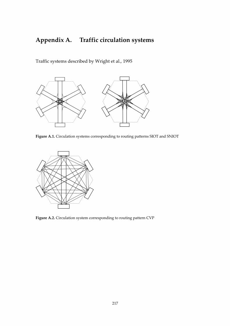
217
Appendix A. Traffic circulation systems
Traffic systems described by Wright et al., 1995
Figure A.1. Circulation systems corresponding to routing patterns SIOT and SNIOT
Figure A.2. Circulation system corresponding to routing pattern CVP
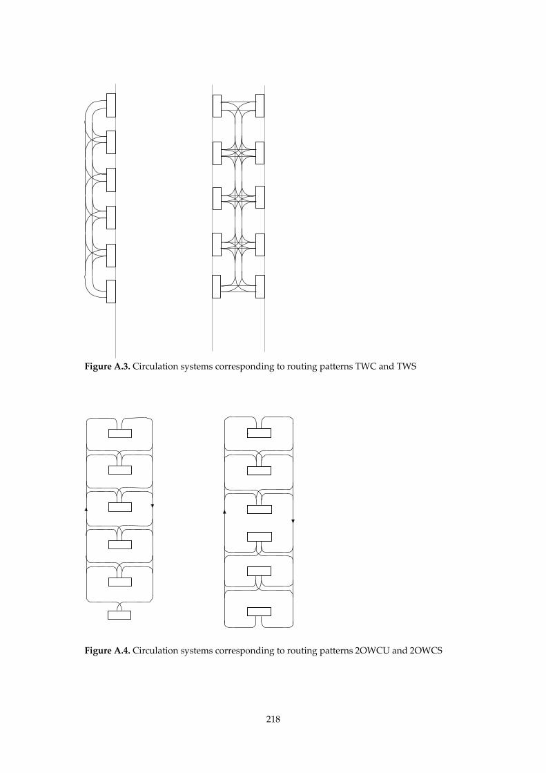
218
Figure A.3. Circulation systems corresponding to routing patterns TWC and TWS
Figure A.4. Circulation systems corresponding to routing patterns 2OWCU and 2OWCS
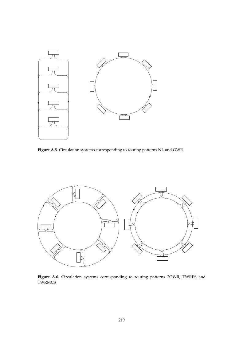
219
Figure A.5. Circulation systems corresponding to routing patterns NL and OWR
Figure A.6. Circulation systems corresponding to routing patterns 2OWR, TWRES and
TWRMCS
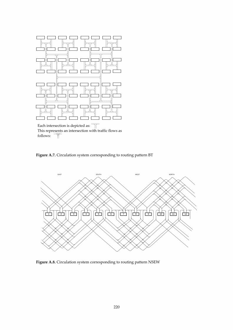
220
Each intersection is depicted as:
This represents an intersection with traffic flows as
follows:
Figure A.7. Circulation system corresponding to routing pattern BT
SOUTHEAST WEST NORTH
1 2 3 4 5 6 7 8 9 10 11 12
Figure A.8. Circulation system corresponding to routing pattern NSEW
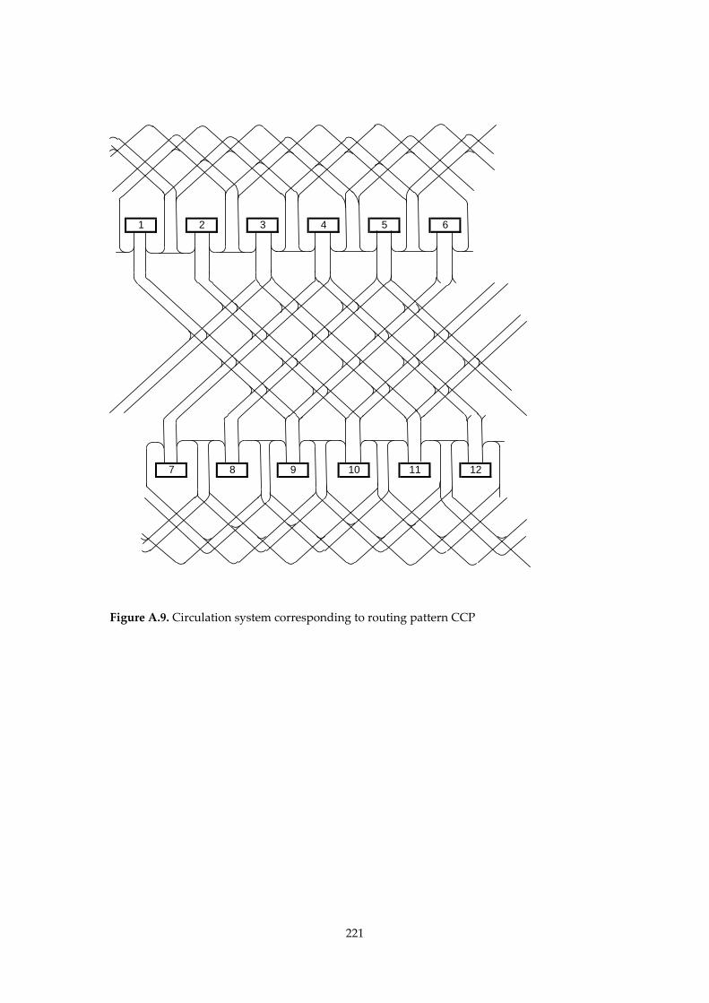
221
5 61 2 3 4
11 127 8 9 10
Figure A.9. Circulation system corresponding to routing pattern CCP
222
Appendix B. Distribution of conflict scores
0.0
10.0
20.0
30.0
40.0
50.0
60.0
70.0
80.0
90.0
100.0
0.00 0.10 0.20 0.30 0.40 0.50 0.60 0.70 0.80 0.90 1.00 1.10 1.20 1.30
Conflicts per kilometre
%
max DVscore
min DVscore
Figure B.1. Distribution of the number of conflicts per unit of length, regarding minimum
and maximum DV scores within an OD pair
0.0
10.0
20.0
30.0
40.0
50.0
60.0
70.0
80.0
90.0
100.0
0.0 0.2 0.4 0.6 0.8 1.0 1.2 1.4 1.6 1.8 2.0
Conflicts per kilometre
% max wghDVscoremin wghDVscore
Figure B.2a. Distribution of the number of conflicts per unit of length, regarding minimum
and maximum wghDV scores within an OD pair
223
0.0
10.0
20.0
30.0
40.0
50.0
60.0
70.0
80.0
90.0
100.0
0.0 150.0 300.0 450.0 600.0 750.0 900.0 1050.0 1200.0 1350.0 1500.0
Conflicts per vehicle kilometre
%
max wghDVscore
min wghDVscore
Figure B.2b. Distribution of the number of conflicts per vehicle kilometre, regarding
minimum and maximum wghDV scores within an OD pair
224
Appendix C. Examples of integrated network design
Figure C.1. Distant regions, regions, and clusters types 1 and 2
D
C
E
F
A
= K1
R
= K2
B
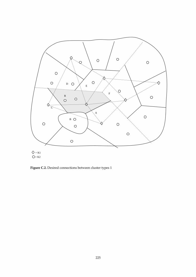
225
Figure C.2. Desired connections between cluster types 1
D
C
E
F
A
= K1
R
= K2
B
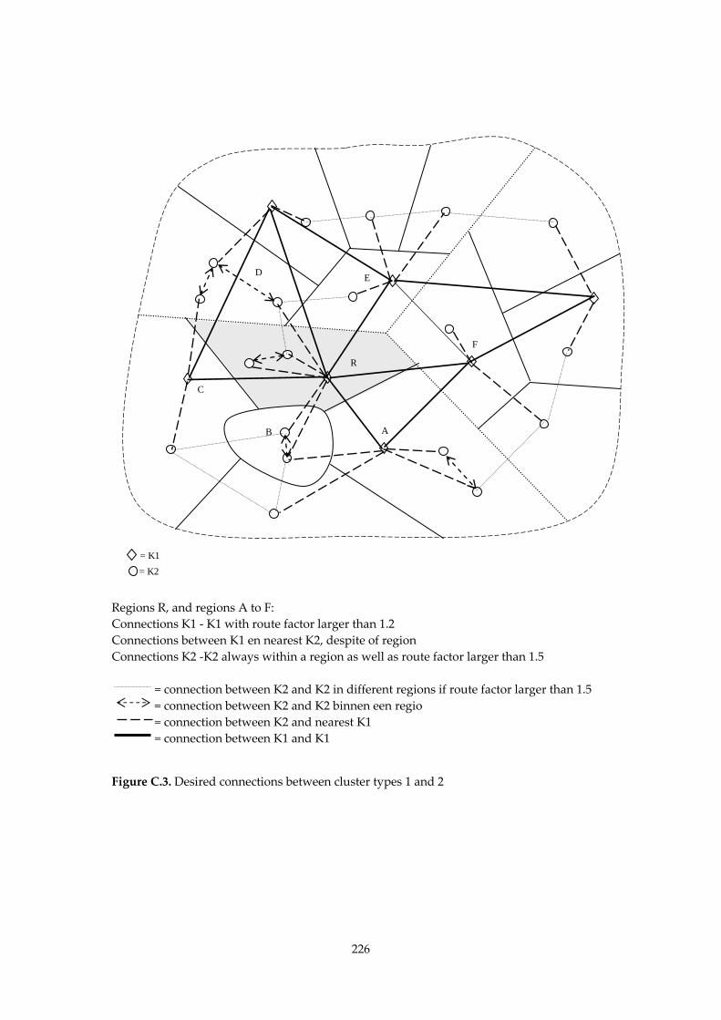
226
Regions R, and regions A to F:
Connections K1 ‐ K1 with route factor larger than 1.2
Connections between K1 en nearest K2, despite of region
Connections K2 ‐K2 always within a region as well as route factor larger than 1.5
= connection between K2 and K2 in different regions if route factor larger than 1.5
= connection between K2 and K2 binnen een regio
= connection between K2 and nearest K1
= connection between K1 and K1
Figure C.3. Desired connections between cluster types 1 and 2
D
C
E
F
A
= K1
R
= K2
B
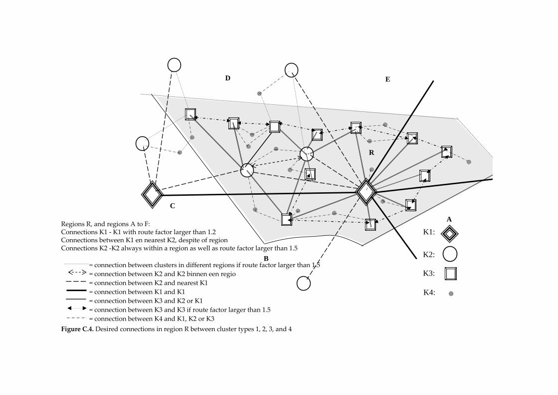
D
C
E
A
R
B
Regions R, and regions A to F: Connections K1 ‐ K1 with route factor larger than 1.2 Connections between K1 en nearest K2, despite of region Connections K2 ‐K2 always within a region as well as route factor larger than 1.5
= connection between clusters in different regions if route factor larger than 1.5
= connection between K2 and K2 binnen een regio
= connection between K2 and nearest K1
= connection between K1 and K1
= connection between K3 and K2 or K1
= connection between K3 and K3 if route factor larger than 1.5
= connection between K4 and K1, K2 or K3
Figure C.4. Desired connections in region R between cluster types 1, 2, 3, and 4
K1:
K2:
K3:
K4:
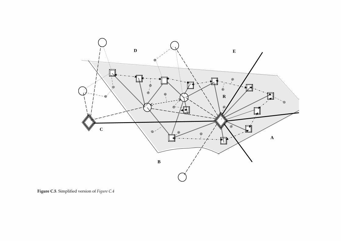
Figure C.5. Simplified version of Figure C.4
D
C
E
A
R
B
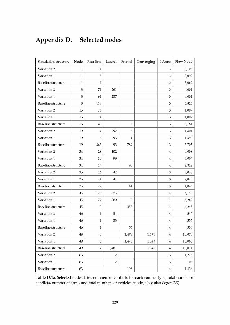
229
Appendix D. Selected nodes
Simulation structure Node Rear End Lateral Frontal Converging # Arms Flow Node
Variation 2 1 11 3 3,105
Variation 1 1 8 3 3,092
Baseline structure 1 9 3 3,067
Variation 2 8 71 261 3 4,001
Variation 1 8 61 257 3 4,001
Baseline structure 8 114 3 3,823
Variation 2 15 76 3 1,007
Variation 1 15 74 3 1,002
Baseline structure 15 40 2 3 3,181
Variation 2 19 4 292 3 3 1,401
Variation 1 19 6 293 4 3 1,399
Baseline structure 19 363 93 789 3 3,705
Variation 2 34 28 102 4 4,008
Variation 1 34 30 99 4 4,007
Baseline structure 34 27 90 4 3,823
Variation 2 35 26 42 3 2,030
Variation 1 35 24 41 3 2,029
Baseline structure 35 22 41 3 1,846
Variation 2 45 126 375 4 4,155
Variation 1 45 177 380 2 4 4,269
Baseline structure 45 10 358 4 4,245
Variation 2 46 1 54 4 545
Variation 1 46 1 53 4 555
Baseline structure 46 1 55 4 530
Variation 2 49 8 1,478 1,171 4 10,078
Variation 1 49 8 1,478 1,143 4 10,060
Baseline structure 49 7 1,481 1,141 4 10,011
Variation 2 63 2 3 1,278
Variation 1 63 2 3 106
Baseline structure 63 196 4 1,436
Table D.1a. Selected nodes 1‐63: numbers of conflicts for each conflict type, total number of
conflicts, number of arms, and total numbers of vehicles passing (see also Figure 7.3)
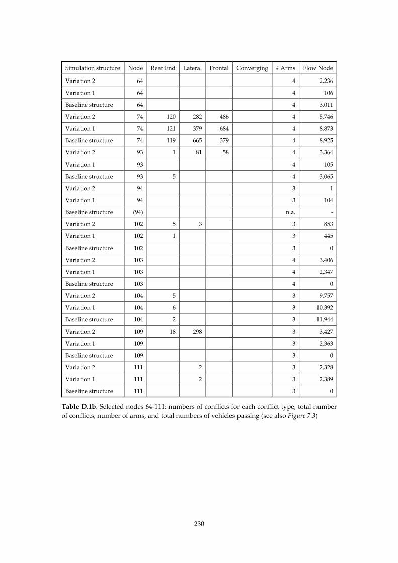
230
Simulation structure Node Rear End Lateral Frontal Converging # Arms Flow Node
Variation 2 64 4 2,236
Variation 1 64 4 106
Baseline structure 64 4 3,011
Variation 2 74 120 282 486 4 5,746
Variation 1 74 121 379 684 4 8,873
Baseline structure 74 119 665 379 4 8,925
Variation 2 93 1 81 58 4 3,364
Variation 1 93 4 105
Baseline structure 93 5 4 3,065
Variation 2 94 3 1
Variation 1 94 3 104
Baseline structure (94) n.a. ‐
Variation 2 102 5 3 3 853
Variation 1 102 1 3 445
Baseline structure 102 3 0
Variation 2 103 4 3,406
Variation 1 103 4 2,347
Baseline structure 103 4 0
Variation 2 104 5 3 9,757
Variation 1 104 6 3 10,392
Baseline structure 104 2 3 11,944
Variation 2 109 18 298 3 3,427
Variation 1 109 3 2,363
Baseline structure 109 3 0
Variation 2 111 2 3 2,328
Variation 1 111 2 3 2,389
Baseline structure 111 3 0
Table D.1b. Selected nodes 64‐111: numbers of conflicts for each conflict type, total number
of conflicts, number of arms, and total numbers of vehicles passing (see also Figure 7.3)
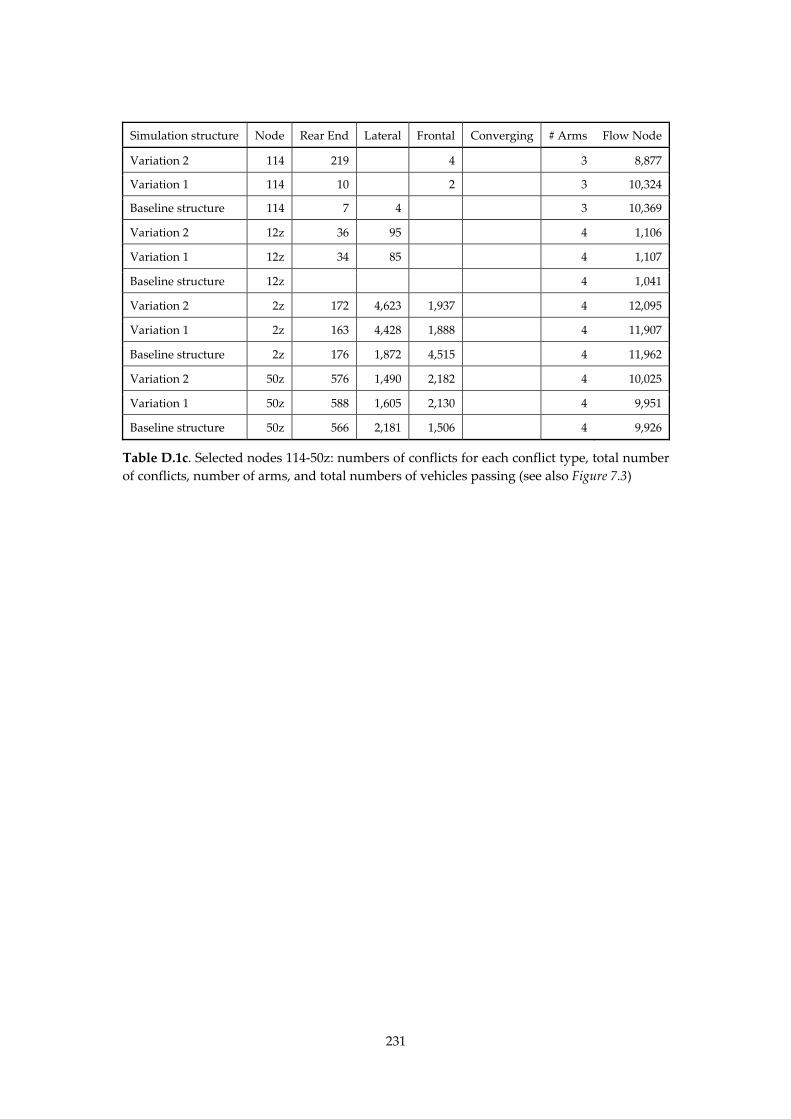
231
Simulation structure Node Rear End Lateral Frontal Converging # Arms Flow Node
Variation 2 114 219 4 3 8,877
Variation 1 114 10 2 3 10,324
Baseline structure 114 7 4 3 10,369
Variation 2 12z 36 95 4 1,106
Variation 1 12z 34 85 4 1,107
Baseline structure 12z 4 1,041
Variation 2 2z 172 4,623 1,937 4 12,095
Variation 1 2z 163 4,428 1,888 4 11,907
Baseline structure 2z 176 1,872 4,515 4 11,962
Variation 2 50z 576 1,490 2,182 4 10,025
Variation 1 50z 588 1,605 2,130 4 9,951
Baseline structure 50z 566 2,181 1,506 4 9,926
Table D.1c. Selected nodes 114‐50z: numbers of conflicts for each conflict type, total number
of conflicts, number of arms, and total numbers of vehicles passing (see also Figure 7.3)

233
Summary
The subject of this study is about the influence of network structure and road
classification on road safety. Road safety, or unsafety, is usually expressed as
the number of crashes or casualties. It is not evident how one can relate what
happens at street level to the decisions regarding network design and the
elaboration of this design. Traffic circulation can be regarded as the link
between these two levels. Behind traffic circulation is the individual who
decides to travel from a point of origin to a destination, using a particular
route. The route is the starting point for this study. That is because network
structure and road classification are important preconditions for traffic
circulation and route choice, while the intersecting routes will determine the
crash locations. This study will therefore focus on the effects of changing
route choices on road safety. The changes in route choice may be the result
of:
1. (intended) changes in the structure of the road network
2. a change in traffic circulation, e.g. on account of an alteration of a traffic
signal system or of congestion on the main roads
3. instructions to car drivers through navigation systems or route
guidance signs
These changes, adaptations and instructions aim to improve the traffic and
transport system as a whole. This study is undertaken to find the effect of the
changes/instructions enumerated above on the safety of all road users in the
road network. This study will show whether an improvement can be
attained and how it can be attained.
In this study, an attempt was made to connect different worlds; the world of
transport network design, the world of route choice research, the world of
micro‐simulation modelling, and finally, the world of surrogate safety
measures (conflict indicators).
The topic of this study was inspired by the functional requirements of
Sustainable Safety, in particular that the shortest and safest route should
coincide. Would it be possible to determine whether this requirement can be
fulfilled? For answering this question, one needs a method that can represent
several safety aspects of trips and routes. Existing methods only show the
safety of either intersections or road sections. New methods had to be
developed for answering the aforementioned questions. These methods are
able to show the results of the improvements for road safety and for traffic
234
flow. The methods can predict the results before the improvements will
actually be implemented.
The topic relates to the following five main research areas: road networks,
use of the road network, routes and route choice, influencing route choice,
and safety aspects of the four previous areas. These main research areas have
been subdivided into eight subjects of this study.
1. Characteristics of transportation networks and road networks; influence on
both the generation of traffic and the circulation of traffic in the road network
Indicators based on the number of crossing or conflicting vehicles and the
type of these conflicts are relevant if road structures need to be selected for
increased road safety. Literature shows a number of indications of some road
structures having low numbers of crossing vehicles. On the other hand, these
structures can have longer distances travelled, which means more exposure
to risk. In theory, some structures have low numbers of crossings as well as
short distances travelled.
2. Road network structure and road classification: their influence on traffic
circulation and its road safety aspects
In the Netherlands, the methods for arriving at a network structure and a
road classification are not a foregone conclusion. The design principles and
rules of thumb are mostly based on practical experience. The scientific
foundation for this set of principles, requirements and rules is very frail.
A series of requirements was formulated in Sustainable Safety with the
purpose of improving the functioning of the road network safety and
efficiency. In this study, the method of ʹintegrated network designʹ was
developed to test whether the road network meets these requirements.
3. Route choice in road networks; options to influence route choice
Car drivers mention ʹfastest routeʹ and ʹshortest routeʹ as main preferences
for their route choice. The next preference is ʹprior knowledge about a routeʹ.
Car drivers hardly ever take ʹsafety of a routeʹ into consideration when
choosing a route. Prior to a trip, most drivers take note of traffic information,
mostly by radio, television or Internet. This information will largely
determine route choice or departure time. The traffic information en route
comes from radio, personal observation, variable message systems, and, for
some drivers, a navigation system. A substantial proportion of drivers
change their route because of this information.
The expected total effect of navigation systems is: less exposure at the
expense of some loss of attention to the other road users.
235
4. Road safety aspects of road network structure and road classification; results
from modelling studies and evaluation studies
Countermeasures regarding network structure and road classification appear
to result in crash or casualty reductions ranging from 40 to 80 percent. In
most cases, safety on the surrounding roads hardly worsened, because
additional measures were taken.
5. Detecting the effects on road safety by changes in route choice; methodological
issues and review of different types of studies
From a series of methods, it can be concluded that a few methods are suited
for studying road safety effects of changes in the use of the road network,
caused by adaptations of the network structure and/or road classification.
The effects of these changes on route choice, in particular, determine the
choice of method. These methods are: key safety indicators, crash prediction
models, comparing features to requirements, and surrogate safety measures
(used in micro‐simulation models). Only surrogate safety measures will
show output for the safety of individual routes.
6. More detailed analysis of road safety indicators; simulated conflicts and
recorded crashes
The estimated numbers of conflicts between vehicles in a micro‐simulation
model (S‐Paramics) have been calculated here according to a specified
method. The number of conflicts at junctions and the number of passing
motor vehicles appear to be quantitatively related to the number of observed
crashes for all junctions. The goodness of fit of this relationship could be
statistically confirmed.
Models like S‐Paramics are, to a great extent, black boxes. For research
purposes, the internal modelling of vehicle movements and interactions
should be clearer.
The model does not yet take traffic other than motor vehicles into account.
Addition of cyclist and pedestrian movements is, however, desired.
7. More detailed analysis of road safety indicators; simulated conflicts, route
characteristics and route criteria
The route score consists of a number of safety criteria. Each criterion can be
weighted. The route scores change slightly if the weighting of the criteria is
adapted. The numbers of conflicts are directly related to the route score. The
weightings are not necessary to improve the relation between route score
and conflict indicators.
236
A high value for the route score is related to a lower number of conflicts, to a
lower conflict density, and to a lower conflict risk.
8. Changing route choice for more safety; adapting road structure.
The application of an integrated network design method to the study area
showed that many connections use roads which have a much higher position
in the road network than desired according to the method. This conclusion
was supported in other (foreign) studies. This finding clearly shows the
structure of the road network in the Netherlands: many main roads
(motorways) facilitating as many connections as possible, disregarding the
distance between the origin and destination of these connections.
Recommendations
This study shows that, in existing road networks, the safest route does not
always coincide with the fastest route. However, car drivers tend to choose
the fastest route. Therefore, the fastest routes should be converted to routes
that are also the safest.
The importance of road classification for road safety purposes seems to be
underestimated. In the Netherlands, the methods for classifying roads could
be improved substantially. This study proposes a method for classifying
roads: integrated network design. Whether this method really benefits road
safety will have to be the subject of further research. This method should be
applied to more areas than the present study area. This may show whether
the results depend on the (type of) area. From these findings, the issues of
generalization and practical application should be resolved.
Road safety will benefit from spreading traffic over a greater number of
roads. However, the cost effectiveness of the increase in road length is still a
matter to be considered.
Another important issue in this study is the safety indicators (surrogate
safety measures). All safety indicators, other than crash figures, are still being
researched. A great deal of study is needed before crash figures can be
replaced by other safety indicators. However, the conflict indicators in micro‐
simulation models appear to be a promising approach in finding adequate
and accurate safety indicators.
The safety criteria of route choice should be incorporated into navigation
systems. A test is recommended to discover the effects of the actual
advantages for safety.
237
Samenvatting
Deze studie gaat over de invloed van netwerkstructuur en wegcategorisering
op verkeersveiligheid. Verkeersveiligheid, of ‐onveiligheid, wordt meestal
uitgedrukt in aantallen slachtoffers of ongevallen. Het is niet duidelijk hoe
men gebeurtenissen op straat kan relateren aan beslissingen op het niveau
van het wegennet of aan de uitwerking daarvan. Verkeerscirculatie
beschouwt men als de verbinding tussen beide niveaus. Achter deze
verkeerscirculatie zit de individuele verkeersdeelnemer die beslist om van
herkomst naar bestemming te reizen, via een specifieke route. De route is het
startpunt van deze studie. Dat is omdat netwerkstructuur en wegcategori‐
sering belangrijke voorwaarden zijn voor de verkeerscirculatie en de
routekeuze. Terwijl de snijpunten van de gekozen routes de ongevalslocaties
bepalen. De studie zal daarom focussen op de veranderingen in routekeuze
op verkeersveiligheid. Veranderingen in routekeuze kunnen plaatsvinden
door:
1. (geplande) veranderingen in de netwerkstructuur;
2. verandering in verkeerscirculatie, bijvoorbeeld door een aanpassing
van een verkeersregelinstallatie of door congestie op hoofdwegen;
3. aanwijzingen aan autobestuurders door een navigatiesysteem of door
aanwijzingen langs de weg.
Deze veranderingen, aanpassingen en aanwijzingen zijn bedoeld om het
verkeerssysteem als geheel te verbeteren. Deze studie is uitgevoerd om het
effect vast te stellen van bovengenoemde veranderingen of aanwijzingen op
de verkeersveiligheid van alle weggebruikers. Deze studie toont aan of een
verbetering wordt bereikt en zo ja, op welke manier.
In deze studie is geprobeerd verschillende werelden te verenigen: de wereld
van het ontwerp van vervoersnetwerken, de wereld van het routekeuze‐
onderzoek, de wereld van microsimulatiemodellen, en ten slotte, de wereld
van de niet‐ongevalgegevens, meestal aangeduid met conflictindicatoren
(ʹsurrogate safety measuresʹ).
Het onderwerp van deze studie is geïnspireerd door de functionele eisen van
Duurzaam Veilig, in het bijzonder de eis dat de veiligste en snelste route
moeten samenvallen. Is het mogelijk om vast te stellen of aan deze eis kan
worden voldaan? Om deze vraag te kunnen beantwoorden is een methode
nodig die uitdrukking geeft aan verschillende veiligheidsaspecten van
verplaatsingen en routes. Bestaande methoden laten alleen de veiligheid van
wegvakken of kruispunten zien, zelden de aaneenschakeling van beide
238
elementen. Nieuwe methoden moesten worden ontwikkeld om de
voorgaande vraagstelling aan te pakken. Deze methoden maken het mogelijk
om het effect van verbeteringen te laten zien op zowel de veiligheid als de
doorstroming van het verkeer. De methoden geven een prognose van de
resultaten voordat de verbeteringen daadwerkelijk tot stand zijn gebracht.
Deze studie richt zich op de volgende onderzoeksgebieden: vervoers‐
netwerken en wegennetten, gebruik van het wegennet, routes en routekeuze,
beïnvloeding van routekeuze, en verkeersveiligheidsaspecten van de
voornoemde gebieden. Deze onderzoeksgebieden zijn onderverdeeld in de
volgende acht onderwerpen.
1. Kenmerken van vervoersnetwerken en wegennetten; invloed op de vervoers‐
vraag en op de verkeerscirculatie in het wegennet
Of een netwerkstructuur voldoende verkeersveilig zal zijn, kan men nagaan
door indicatoren te hanteren die een schatting geven van het aantal
kruisende of conflicterende voertuigen en/of van de voorkomende conflict‐
typen. De literatuur laat zien dat in sommige netwerkstructuren een gering
aantal kruisende voertuigen mag worden verwacht. Anderzijds zijn de
afgelegde afstanden dan meestal groter; dat betekent meer blootstelling aan
gevaar. Er zijn echter netwerkstructuren die zowel een gering aantal
kruisende voertuigen als kortere afgelegde afstanden vertonen.
2. Netwerkstructuur en wegcategorisering; hun invloed op de verkeerscirculatie
en hun verkeersveiligheidsaspecten
In Nederland is het nog geen uitgemaakte zaak welke methoden geschikt
zijn om de netwerkstructuur en de wegcategorisering respectievelijk te
ontwerpen en vast te stellen. De gehanteerde ontwerpprincipes en vuist‐
regels zijn voornamelijk gebaseerd op praktijkervaring. De wetenschappe‐
lijke onderbouwing voor deze principes, eisen en vuistegels is zeer zwak.
In Duurzaam Veilig is een pakket van eisen geformuleerd met als doel het
wegennet veiliger en efficiënter te laten functioneren. In deze studie is de
kernenmethode ontwikkeld om na te gaan of het wegennet voldoet aan de
gestelde eisen.
3. Routekeuze in wegennetten; mogelijkheden om routekeuze te beïnvloeden
Autobestuurders noemen ʹsnelste routeʹ en ʹkortste routeʹ als de belangrijkste
voorkeuren bij hun routekeuze. De derde voorkeur is ʹvoorgaande kennis
over een routeʹ. Autobestuurders letten bij hun routekeuze zelden op
ʹveiligheid op een routeʹ. Voorafgaand aan een verplaatsing nemen de meeste
bestuurders kennis van verkeersinformatie via radio, televisie of internet.
239
Deze informatie bepaalt in hoofdlijnen de vertrektijd en de routekeuze. De
verkeersinformatie onderweg verkrijgt men via de radio, eigen observatie,
dynamische route‐informatie en, voor sommigen, het navigatiesysteem. Een
aanzienlijk deel van de bestuurders verandert de route op grond van deze
informatie.
Het verwachte totale effect van navigatiesystemen is: minder blootstelling
aan gevaar ten koste van enig verlies aan aandacht voor andere weg‐
gebruikers.
4. Verkeersveiligheidsaspecten van netwerkstructuren en van wegcategorisering;
resultaten uit modelstudies en evaluatiestudies
Maatregelen op het niveau van netwerkstructuur en wegcategorisering
hebben in de praktijk geleid tot grote dalingen (40 tot 80 procent) in het
aantal verkeersslachtoffers. In de meeste gevallen is de onveiligheid op de
omliggende wegen van deze aangepaste gebieden nauwelijks verslechterd
doordat aanvullende maatregelen waren genomen.
5. Het veiligheidseffect van een veranderde routekeuze vaststellen; methodo‐
logische kwesties en een overzicht van diverse studies
Uit een aantal verschillende studies kan worden afgeleid dat er enkele
geschikte methoden zijn om de veiligheidseffecten te bepalen van
veranderingen in het gebruik van het wegennet. Dit betreft veranderingen
die veroorzaakt zijn door aanpassingen van de netwerkstructuur en/of de
wegcategorisering. De hier gezochte methoden moeten inzicht bieden in het
effect van veranderingen op de routekeuze. Deze methoden zijn: risicocijfers,
ʹcrash prediction modelsʹ, vergelijking van verkeersvoorzieningen met de
gestelde verkeerskundige eisen, en veiligheidsindicatoren die in micro‐
simulatiemodellen worden gebruikt (ʹsurrogate safety measuresʹ). Alleen de
laatstgenoemde methode laat de veiligheid van individuele routes zien.
6. Gedetailleerde analyse van veiligheidindicatoren; gesimuleerde conflicten en
geregistreerde ongevallen
De aantallen conflicten tussen voertuigen in het hier gebruikte micro‐
simulatiemodel (S‐Paramics) zijn geschat volgens een methode die in deze
studie is beschreven. Het aantal geschatte conflicten op kruispunten is
gerelateerd aan het aantal geregistreerde ongevallen op die kruispunten.
Hiertussen blijkt een kwantitatieve relatie te bestaan; dit is statistisch
onderbouwd.
Modellen zoals S‐Paramics zijn in grote mate een ʹblack boxʹ. Voor
onderzoeksdoeleinden zou er meer duidelijkheid moeten komen over de
240
modellering van de bewegingen van de voertuigen en van de onderlinge
reacties tussen de voertuigen.
In het gebruikte model zijn alleen motorvoertuigen beschouwd. Toevoeging
van fietsers en voetgangers is wenselijk.
7. Gedetailleerde analyse van veiligheidsindicatoren; gesimuleerde conflicten,
kenmerken van routes en routecriteria
De zogeheten routescore bestaat uit een aantal veiligheidscriteria. Elk
criterium kan worden voorzien van een weegfactor waardoor de onderlinge
verhoudingen tussen de weegfactoren veranderen. De routescores ver‐
anderen in geringe mate bij toepassing van deze weegfactoren. De
routescores zijn direct gerelateerd aan het geschatte aantal conflicten per
route. Het gebruik van weegfactoren beïnvloedt deze relatie nauwelijks.
Een hoge waarde van de routescore zou theoretisch overeen moeten komen
met een laag aantal conflicten, met een lage conflictdichtheid en met een laag
conflictrisico. Dit blijkt volgens de geanalyseerde gegevens het geval te zijn.
8. De routekeuze veranderen om de veiligheid te bevorderen; aanpassing van de
netwerkstructuur
De toepassing van de kernenmethode op het studiegebied laat zien dat veel
verbindingen tussen kernen via wegen verlopen die een veel hogere functie
in het netwerk hebben dan voor die verbindingen (volgens de methode)
gewenst is. Deze conclusie is ook in andere (buitenlandse) studies getrokken.
Deze bevinding laat zien dat het Nederlandse wegennet een structuur heeft
die bestaat uit relatief veel autosnelwegen met veel aansluitingen en dat veel
routes via deze wegen lopen, ongeacht de afstand van verplaatsing.
Aanbevelingen
Deze studie laat zien dat in bestaande wegennetten de veiligste route niet
altijd via de snelste route loopt. Autobestuurders kiezen echter meestal voor
de snelste route. Daarom zouden de snelste routes moeten worden aangepast
zodat ze ook de veiligste worden.
Het belang van wegcategorisering voor veiligheidsdoeleinden wordt
onderschat. In Nederland kan de methode om wegen te categoriseren flink
worden verbeterd door de kernenmethode toe te passen. Of deze methode
daadwerkelijk de veiligheid zal verbeteren verdient nadere studie. In deze
studie is de methode toegepast op één studiegebied; toepassing op meer
gebieden is gewenst. Daaruit zal blijken of de methode generaliseerbaar is.
Vervolgens is een bredere toepassing aan de orde.

241
De verkeersveiligheid is ermee gediend om het verkeer over verschillende
routes te spreiden. Onderzoek is gewenst naar de maatschappelijke
kosteneffectiviteit hiervan.
In deze studie zijn veiligheidsindicatoren gebruikt, met name conflict‐
indicatoren en routescores. Alle veiligheidsindicatoren, anders dan
ongevallencijfers, zijn (internationaal) onderwerp van onderzoek. Uit de
resultaten van dat onderzoek moet blijken of het verantwoord is om
veiligheidsindicatoren in plaats van ongevallencijfers te hanteren. Uit deze
studie blijkt dat conflictindicatoren sterk gerelateerd zijn aan ongevallen‐
cijfers. Dit is een belangrijke stap op weg naar adequate veiligheids‐
indicatoren.
De hier gehanteerde veiligheidscriteria voor routekeuze kunnen ingebouwd
worden in navigatiesystemen. In een pilotstudie kunnen de werkelijke
effecten hiervan op veiligheid worden onderzocht.

243
Curriculum Vitae
Atze Dijkstra was born in Groningen, on 19 November 1954. He studied civil
engineering at the Delft University of Technology. After his graduation, he
worked as a researcher at the Transportation and Traffic Engineering Section
of the Faculty of Civil Engineering. In 1983 he joined the SWOV Institute for
Road Safety Research as a researcher, a post he fulfilled until 1992. His main
research projects dealt with the analysis of the safety aspects of bicycle
facilities, the evaluation of 30 km/h zones, and the analysis of quantitative
relations between road characteristics (of main rural and urban roads) and
crash indicators. When he left SWOV in 1992, he was a project manager
responsible for the research programme ʹDesigning safer roadsʹ.
From 1992 until 1996 he worked as a researcher and research manager at the
OTB Research Institute for Housing, Urban and Mobility Studies (an institute
of the Delft University of Technology). His work focused on both goods
transport by rail (evaluation of the existing capacity of the rail
infrastructure), and on internal goods transport, using the Maasvlakte (Port
of Rotterdam) as a case study.
He rejoined the SWOV as a senior researcher in 1996. From 1996 to 1998 he
was the project manager of several work packages in European research
projects regarding bicycle and pedestrian facilities (ADONIS), and regarding
the design of road infrastructure (SAFESTAR). SAFESTAR was also the
platform from which Road Safety Audits in the Netherlands were launched.
He set up the national course for road safety auditors; a course that has been
presented every year since 2001.
From 1999 to 2003 he was the manager of the research programme ʹRoad
design and road safetyʹ. Within this programme he set up and supervised the
evaluation of the newly built 60 km/h zones. In this period, Atze was a
member of a number of national working groups (organized by CROW) on
various geometrical and related topics (incl. road humps, bicycle facilities,
pedestrian crossings).
At the end of 2003 Atze started working on the project ʹRoute choice in a
road networkʹ which ultimately resulted in his thesis. This eight‐year project
was an opportunity for him to get extensively acquainted with the intricacies
of micro‐simulation modelling. During this period, he also wrote many fact
sheets, evaluated the safety of bicycle facilities at roundabouts, and studied
the effects of a robust road network on road safety.

245
SWOV‐Dissertatiereeks
In deze reeks zijn eerder verschenen:
Jolieke Mesken (2006). Determinants and consequences of driversʹ emotions.
Ragnhild Davidse (2007). Assisting the older driver: Intersection design and in‐car
devices to improve the safety of the older driver.
Maura Houtenbos (2008). Expecting the unexpected: A study of interaction
behaviour at intersections.
Frits Bijleveld (2008). Time series analysis in road safety research using state space
methods.
Saskia de Craen (2010). The X‐factor; A longitudinal study of calibration in young
novice drivers.

En route to safer roads
Atze Dijkstra
En
route to safer road
s A
tze Dijkstra
ISB
N: 978-90-73946-08-8
How road structure and road classificationcan affect road safety