empirical evidence on the importance of aggregation

Empirical Evidence on the Importance ofAggregation, Asymmetry, andJumps for Volatility Prediction*

Diep Duong1and Norman R. Swanson21Utica College and 2Rutgers University

June 2014

Abstract

Many recent modelling advances in finance topics ranging from the pricing of volatility-based derivative products

to asset management are predicated on the importance of jumps, or discontinuous movements in asset returns. In light

of this, a number of recent papers have addressed volatility predictability, some from the perspective of the usefulness

of jumps in forecasting volatility. Key papers in this area include Andersen, Bollerslev, Diebold and Labys (2003),

Corsi (2004), Andersen, Bollerslev and Diebold (2007), Corsi, Pirino and Reno (2008), Barndorff, Kinnebrock, and

Shephard (2010), Patton and Shephard (2011), and the references cited therein. In this paper, we review the extant

literature and then present new empirical evidence on the predictive content of realized measures of jump power

variations (including upside and downside risk, jump asymmetry, and truncated jump variables), constructed using

instantaneous returns, i.e., || 0 ≤ ≤ 6, in the spirit of Ding, Granger and Engle (1993) and Ding and Granger(1996). We also present new empirical evidence on the predictive content of realized measures of truncated large jump

variations, constructed using truncated squared instantaneous return, i.e., 2 × || where is the threshold

jump size Our prediction experiments use high frequency price returns constructed using S&P500 futures data as well

as stocks in the Dow 30, and our empirical implementation involves estimating linear and nonlinear heterogeneous

autoregressive realized volatility (HAR-RV) type models. We find that past "large" jump power variations help

less in the prediction of future realized volatility, than past "small" jump power variations. Additionally, we find

evidence that past realized signed jump power variations, which have not previously been examined in this literature,

are strongly correlated with future volatility, and that past downside jump variations matter in prediction. Finally,

incorporation of downside and upside jump power variations does improve predictability, albeit to a limited extent.

JEL Classification: C58, C53, C22.

Keywords: realized volatility, jump power variations, downside risk, semivariances, market mi-

crostructure, volatility forecasts, jump test.

∗Diep Duong, Utica College, 1600 Burrstone Road, Utica, NY 13502, USA, [email protected]. Norman R. Swanson, De-partment of Economics, Rutgers University, 75 Hamilton Street, New Brunswick, NJ 08901, USA, [email protected].

The authors wish to thank the editor, Michael McAleer, for providing much guideance and many useful comments on earlier

versions of this paper. Additionally, we wish to thank two anonymous referees, Valentina Corradi, Roger Klein, John Landon-

Lane, Richard McLean, George Tauchen and participants at workshops given at the Bank of Canada, East Carolina University,

Rutgers University, and Utica College for many useful comments and discussions.

1 Introduction

Many recent modelling advances in asset pricing and management are predicated on the impor-

tance of jumps, or discontinuous movements in asset returns. Indeed, if jumps are found to be

present in the data, the economic implications of including jump processes in dynamic asset pricing

exercises are substantial. For example, the incorporation of jumps leads to break-downs in typical

market completeness conditions needed for portfolio replication strategies in derivatives valuations.

Additionally, jumps complicate the implementation of "state of the art" change of risk measures

in risk neutral pricing. As a result, asset allocation and risk management, which heavily depend

on risk measures and underlying asset return dynamics, are affected. In volatility measurement, it

is necessary to separate out the volatility due to jumps or construct variables that appropriately

summarize information generated by jumps. The above considerations are of particular importance,

given recent evidence on the importance of jumps, both "finite activity jumps" (see e.g., Huang

and Tauchen (2005)) and "infinite activity jumps" (see e.g., Aït-Sahalia and Jacod (2009b)) that

is reported in the literature.1

In this paper, we add to the empirical literature on volatility prediction by carrying out a

series of experiments in order to ascertain the usefulness of a variety of jump variables, including

realized measures of jump power variations that are designed to estimate upside and downside risk,

jump asymmetry, and truncated "large" jumps, for example. Key earlier related papers include

Andersen, Bollerslev, Diebold and Labys (2003), Corsi (2004), Andersen, Bollerslev and Diebold

(ABD: 2007), Corsi, Pirino and Reno (2008), Barndorff, Kinnebrock, and Shephard (BKS: 2010),

Patton and Shephard (PS: 2011), and the references cited therein.

There are two ingredients in the experiments that we carry out. The first ingredient involves

the choice of volatility estimator. One available estimator is based on "backing out" volatility

from parametric ARCH, GARCH, stochastic volatility, or derivatives pricing models. Another

estimator, which we use, is "model free". Examples include realized volatility (RV), as examined in

the seminal paper by Andersen, Bollerslev, Diebold and Labys (2001), and variants thereof such as

bipower variation, tripower variation, multipower variation, semivariance, and various others.2 One

reason for the use of model free realized measures (RMs), is that they allow us to treat volatility

as if it is observed, when we subsequently fit regressions in order to assess predictability. 3 The

RMs that we implement are predicated on recent theoretical advances due to Jacod (2008), BKS

1For other examples of work in this area, see Aït-Sahalia (2002), Carr, Geman, Madan, Yor (2002), Barndorff-

Nielsen and Shephard (2004, 2006), Cont and Mancini (2007), Jacod (2008), Jiang and Oomen (2008), Lee and

Mykland (2008), Aït-Sahalia and Jacod (2009a), Todorov and Tauchen (2010), and the references cited therein.2See Barndorff-Nielsen and Shephard (2004), Aït-Sahalia, Mykland and Zhang (2005), Zhang (2006), Barndorf-

Nielsen, Hansen, Lunde, and Shephard (2008), Jacod (2008), BKS (2010), and the references cited therein.3Modeling and forecasting RMs is important not only because RMs are natural proxies for volatility, but also

because of the many practical applications and uses of RMs in constructing synthetic measures of risk in the financial

markets (see e.g., Duong and Swanson (2011) for a discussion of the VIX and other derivatives constructed using

RMs). Additionally, see Andersen, Bollerslev, Diebold and Labys (2003), Corsi (2004), and ABD (2007), and Corradi,

Distaso and Swanson (2009, 2011) for a discussion of prediction using RMs.

1

(2010), Todorov and Tauchen (2010), and Aït-Sahalia and Jacod (2012). In particular, the limit

theory that we adopt allows us to use RMs to construct estimators of downside and upside jump

power variations using intra-daily positive and negative returns. These estimators are suggested

by BKS (2010) as alternatives to the semivariances implemented in Patton and Shephard (2011).

We also examine jump asymmetry (i.e., realized signed jump power variation).

The second ingredient involves which variables to use to measure jumps. Once jumps are

found, one approach to capture large jump variations is to use the jump decomposition technique

implemented in Duong and Swanson (2011) to construct realized measures (RMs) of the variational

contribution of large and small jumps to total variation. Another approach, which is the main focus

of this paper is to examine various different RMs of jump power variations, formed using power

transformations of the instantaneous return, i.e., ||. The analysis of power transformations

of returns is not new. Ding, Granger and Engle (1993) and Ding and Granger (1996) develop

long memory asymmetric power ARCH models based on power transformations of daily absolute

returns. They find that the autocorrelations of power transformations of S&P500 returns are the

strongest for 1. In the context of high frequency data, Liu and Maheu (2005) and Ghysels

and Sohn (GS: 2009) study the predictability of future realized volatility using past absolute power

variations and multipower variations. Ghysels and Sohn (2009) find that the optimal value of is

approximately unity. However, their empirical evidence considers the continuous class of models,

and does not account for jumps. In related recent work that is closest to that reported in this

paper, BKS (2010) construct new estimators of downside (and upside) risk (i.e., so-called realized

semivariances), using square transformations of positive and negative intra-daily return, and find

that downside risk measures are important when attempting to model and understand risk They

note, as quoted from Granger (2008), that: ‘It was understood that risk relates to an unfortunate

event occurring, so for an investment this corresponds to a low, or even negative, return. Thus

getting returns in the lower tail of the return distribution constitutes this “downside risk.” However,

it is not easy to get a simple measure of this risk.’ This point is noteworthy, since it is argued in

the literature (see e.g., Ang, Chen and Xing (2006)), that investors treat downside losses differently

than upside gains. 4

Of note is that the role of the size of jumps in forecasting can be gauged (to some extent)

through examination of the order of For this reason, we consider jump power variations with

0 ≤ ≤ 6 While previous authors have focused on ≤ 2 allowing for a wider range of valuesfor is sensible, given that convergence to jump power variation occurs only when 2 (see e.g.,

Todorov and Tauchen (2010) and BKS (2010)). 5 As discussed above, our prediction experiments

4 In the parametric framework, some authors also develop approaches to modeling time-varying higher order

conditional moments (see e.g., Timmermann (2000) and Perez-Quiros and Timmermann (2001). Maheu and Curdy

(2004) take this sort of analysis one step further and incorporate past jumps as a new source of asymmetry, and find

improved volatility forecastability.5 In our implementation, prediction results for 6 are qualitatively the same as those for = 6 and are therefore

not reported on.

2

are designed to separately analyze "large" and "small" jumps using jump power variation RMs.

For completeness, we also analyze jumps using RMs of truncated large jump variations. These

are constructed using squared instantaneous returns, i.e., 2 × || where || is an indicatortaking the value 1 if || and 0 otherwise. Analogous to the choice of large jumps variations

depend on the truncation level 0. A grid search is carried out in order to provide evidence on

"optimal" values for use in volatility prediction.

The dataset used in our empirical investigation consists of high frequency price returns con-

structed using S&P500 futures index data for the period 1993-2009, as well as stocks in the Dow 30,

for the period 1993-2008; and our empirical implementation involves estimating linear and nonlinear

extended heterogeneous autoregressive realized volatility (HAR-RV) type models. Our findings can

be summarized as follows. First, we find evidence that jumps characterize the structure of both the

S&P500 futures index and the individual stocks that we examine. Second, our experiments indicate

accuracy improvements, both in- and out-of-sample, when RMs of jump power variations are used

as additional predictors in HAR-RV type models. However, past "large" jump power variations help

less in the prediction of future realized volatility, than past "small" jump power variations. In a

related finding, we note that seemingly rare and possibly jumps do not help in prediction, while

smaller, less rare and possibly serially correlated jumps do help. Third, the continuous component

dominates in all prediction experiments, which is consistent with previous findings in the literature

on volatility forecasting using high frequency data. Fourth, incorporation of downside and upside

jump power variations does improve predictability, albeit to a limited extent. Fifth, comparing "no

jump test" cases with "jump test" cases indicates that findings do change, to some degree, when

jump tests are used in the construction of jump variation variables. Additionally, the power of

associated with our 2−"best" model is higher when S&P500 index returns are predicted, thanwhen individual DOW components are predicted. This suggests that aggregation plays a role in

risk prediction. Values of less than 2 dominate for individual stocks, while values greater than

2 dominate for our index variable. Finally, our prediction experiments based on the use of RMs

of truncated large jump variations constructed using the jump decomposition approach (see above

discussion) are consistent with the above finding that larger jump variations help less in the pre-

diction of future realized volatility than smaller jump variations. In particular, out-of-sample 2

values associated with the grid of truncation levels, are monotonically decreasing in .

A general finding that permeates all of our experiments is that what’s best for in-sample analysis

is far from best for out-of-sample analysis. Another general finding is that jumps do play a role,

at least when modelling aggregate (index) data such as S&P500 futures returns; and while jump

risk power variations may not be important for in-sample fit, they clearly play an important role

in out-of-sample volatility prediction.

The rest of the paper is organized as follows. Section 2 discusses volatility and jumps, while

Section 3 discusses the various realized measures of price jump variation that we examine. Section 4

3

outlines our experimental setup, and Section 5 gathers our empirical findings. Concluding remarks

are contained Section 6.

2 Volatility and Price Jump Variations

2.1 Set-up

We adopt a general semi-parametric specification for asset prices. Following Todorov and Tauchen

(2010), the log-price of asset, = log() is assumed to be an Itô semimartingale process,

= 0 +

Z

0

+

Z

0

+ (1)

where 0 +R 0+

R 0 is a Brownian semi-martingale and is a pure jump process which

is the sum of all "discontinuous" price movements up to time

=X≤∆

is assumed to be finite6 and a jump at time is defined as ∆ = − −.

When the jump component is a compound Poisson process (CPP) - i.e. a finite activity jump

process - then,

=

X=1

(2)

where is number of jumps on [0 ]. follows a Poisson process, and the jump magnitudes,

i.e. the 0 are random variables. The CPP assumption has been widely used in the literature

on modeling, forecasting, and testing for jumps. However, jumps may arise in other model setups,

such as when infinite activity jumps are specified (see Todorov and Tauchen (2010)).

The empirical evidence discussed in this paper involves examining the variation of the log-price

jump component using an equally spaced path of historically observed prices, i.e. {0 1∆ 2∆ ∆},where the sampling frequency, ∆ =

is deterministic. The intra-daily return or increment of

is

= ∆ − (−1)∆

Returns are observed at various frequencies. However, volatility of log-prices is often treated as

an unobserved variable. The "true" price variance (risk) is defined in this paper by the quadratic

variation of the process , i.e.,

= [ ] =

Z

0

2+

6See, for example Jacod (2008) or Todorov and Tauchen (2010) for the conditions for the finiteness of jumps.

4

where the variation of the continuous component (integrated volatility) is

=

Z

0

2

and the variation of the price jump component is

=X≤(∆)

2

Realized volatility (RV), is constructed by simply summing up all successive intra-daily squared

returns, and converges to the quadratic variation of the process, as →∞ 7,

=

X=1

2−→ = + (3)

where ucp denotes uniform convergence in probability.

2.2 Jump Tests and Jump Decompositions

In this section, we review results on jump tests applied in this paper and the jump decomposition

approach used in Duong and Swanson (2011) and Aït-Sahalia and Jacod (2012).

2.2.1 Testing for Jumps

Jump detection is useful as a "pre-test", prior to constructing RMs of jump and continuous com-

ponents of a variable. We implement the jump test methodology of Huang and Tauchen (2005)

and BNS (2006), extended to processes such as (1).8 The key point of the test methodology is that

under the null hypothesis of no jumps, the difference between the estimators of variation of the

continuous component and total quadratic variation should be close to 0. We follow the empirical

strategy in Duong and Swanson (2011) in which adjusted jump ratio statistics developed by Huang

and Tauchen (2005) are used, i.e.,

=

pq

(−1d(c )2)

Ã1−

c P=1()

2

!−→ (0 1)

7This is a standard result in high frequency econometrics. For instance, see Todorov and Tauchen (2010).8As discussed in Duong and Swanson (2011), the extension is based on limit theorems recently developed by Jacod

(2008) and Aït-Sahalia and Jacod (2009a). For instance, let () = , let be the law (0 2) and let ()

be the integral of with respect to this law. Then:1

∆

∆

=1

(√∆

)2 −

0

()

−−→

0

(

2)− 2() (4)

Here, − denotes stable convergence in law, which also implies convergence in distribution. For = 2 the above

theorem is the same as BNS (2006), which is the key limit theorem for their jump test statistics derivation.

5

where c (tripower variation) and d (multipower variation) are estimators ofR 02 and ofR

04, respectively. In particular,

c = 23 23 23−323

and c = ∆−1 4

3 43 43−343

(5)

where = (||) and is a (0 1) random variable, with

12=

X=2

||1 |−1|2 |−| ,

where 12 are positive, such thatP1 = In general, given a daily test statistic,

() where is the number of observations per day and is the test significance level, we reject

the null hypothesis if () is in excess of the critical value Φ leading to a conclusion that there

are jumps during the day. The converse holds if () Φ.

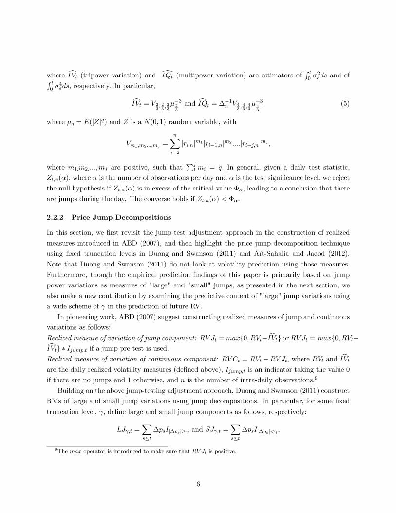
2.2.2 Price Jump Decompositions

In this section, we first revisit the jump-test adjustment approach in the construction of realized

measures introduced in ABD (2007), and then highlight the price jump decomposition technique

using fixed truncation levels in Duong and Swanson (2011) and Aït-Sahalia and Jacod (2012).

Note that Duong and Swanson (2011) do not look at volatility prediction using those measures.

Furthermore, though the empirical prediction findings of this paper is primarily based on jump

power variations as measures of "large" and "small" jumps, as presented in the next section, we

also make a new contribution by examining the predictive content of "large" jump variations using

a wide scheme of in the prediction of future RV.

In pioneering work, ABD (2007) suggest constructing realized measures of jump and continuous

variations as follows:

Realized measure of variation of jump component: ={0 −c} or = {0 −c} ∗ if a jump pre-test is used.

Realized measure of variation of continuous component: = − where and care the daily realized volatility measures (defined above), is an indicator taking the value 0

if there are no jumps and 1 otherwise, and is the number of intra-daily observations.9

Building on the above jump-testing adjustment approach, Duong and Swanson (2011) construct

RMs of large and small jump variations using jump decompositions. In particular, for some fixed

truncation level, , define large and small jump components as follows, respectively:

=X≤∆|∆|≥ and =

X≤∆|∆|

9The operator is introduced to make sure that is positive.

6

where |∆|≥ AsP

=1 2||≥ converges uniformly in probability to

P≤(∆)

2|∆|≥ as goes to infinity, the variation of jumps with magnitude larger than and smaller than are

denoted and calculated as follows:10

Realized measure of truncated large jump variation: = min{ P

=1 2||≥} or

= min{ (P

=1 2 ∗ ||≥) ∗ } if jump test is applied.

Realized measure of truncated small jump variation: = − where is

defined above and ||≥ is an indicator taking the value 1 if || ≥ and 0 otherwise.11

3 Jump and Signed Jump Power Variations

In the previous section, we discussed jump variation decompositions using truncation levels. Note

that a key difficulty in the application of this decomposition approach lies in the choice of truncation

levels, which is arbitrary. Although we address this issue to some extent via use of a grid search,

recent theoretical advances suggest that using power variations to measure the contribution of

jumps may prove useful. In particular, recent limit theory developed in the financial econometric

literature allows us to assess jump variations from various spectrum using jump power variations

formulated by power transformation of absolute log-price jumps (|∆|).12 In particular, definethe jump power variation as follows:

=X0≤

|∆|, (6)

with "upside" jump power variation defined as

+ =X0≤

|∆|∆0, (7)

and "downside" jump power variation defined as

− =X0≤

|∆|∆0. (8)

Finally, measure jump asymmetry using so-called signed jump power variation, defined as follows,

=X0≤

|∆|∆0 −X0≤

|∆|∆0. (9)

In the above expressions, we are interested in the case where ≥ 2. Note that for large valuesof

+

− are dominated by large jumps. For 2 the jump variations

are not always guaranteed to be finite. One of our main goals in this paper is to construct and

10See Jacod (2008), Aït-Sahalia and Jacod (2012) for further details.11As done in a related context in ABD (2007), the min operator is introduced to make sure that ≤ 12For further discussion, see above, and refer to Jacod (2008), BKS(2010), Todorov and Tauchen (2010) and

Aït-Sahalia and Jacod (2012).

7

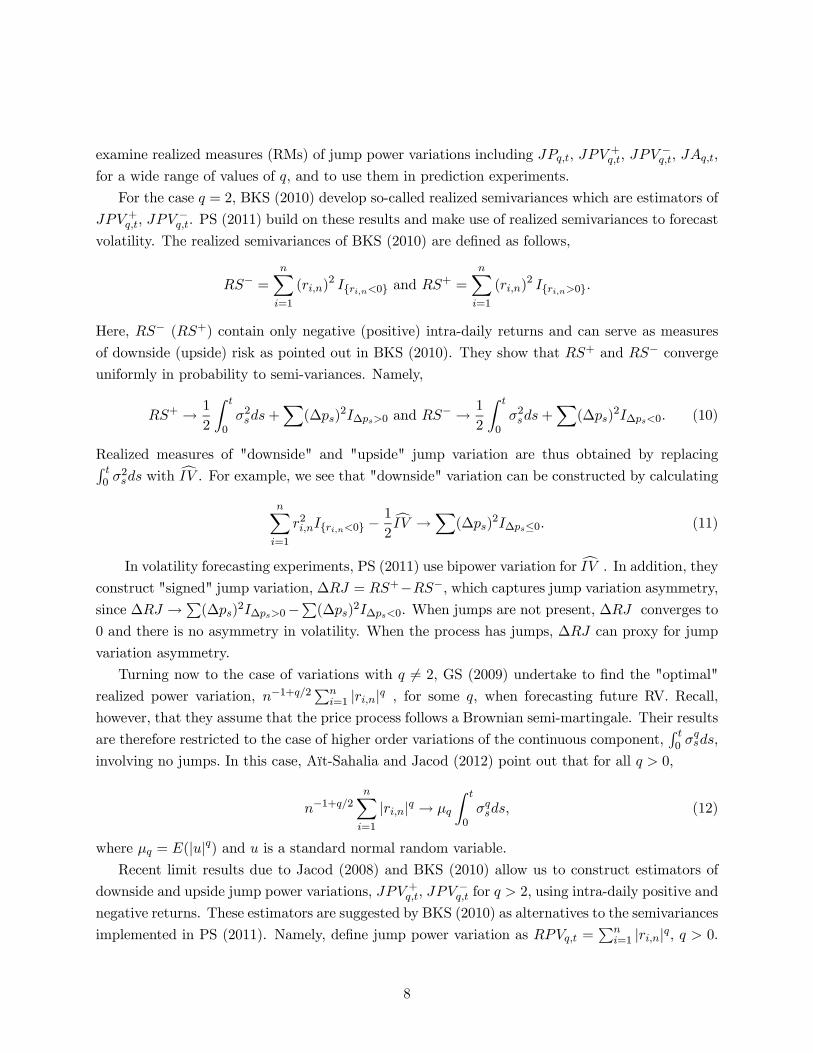
examine realized measures (RMs) of jump power variations including +

−

for a wide range of values of , and to use them in prediction experiments.

For the case = 2, BKS (2010) develop so-called realized semivariances which are estimators of

+ −. PS (2011) build on these results and make use of realized semivariances to forecast

volatility. The realized semivariances of BKS (2010) are defined as follows,

− =X=1

()2 {0} and + =

X=1

()2 {0}.

Here, − (+) contain only negative (positive) intra-daily returns and can serve as measuresof downside (upside) risk as pointed out in BKS (2010). They show that + and − convergeuniformly in probability to semi-variances. Namely,

+ → 1

2

Z

0

2+X(∆)

2∆0 and − → 1

2

Z

0

2+X(∆)

2∆0. (10)

Realized measures of "downside" and "upside" jump variation are thus obtained by replacingR 02 with

c . For example, we see that "downside" variation can be constructed by calculatingX=1

2{0} −1

2c →X

(∆)2∆≤0. (11)

In volatility forecasting experiments, PS (2011) use bipower variation for c . In addition, theyconstruct "signed" jump variation, ∆ = +−− which captures jump variation asymmetry,since ∆ →P

(∆)2∆0−

P(∆)

2∆0. When jumps are not present, ∆ converges to

0 and there is no asymmetry in volatility. When the process has jumps, ∆ can proxy for jump

variation asymmetry.

Turning now to the case of variations with 6= 2 GS (2009) undertake to find the "optimal"realized power variation, −1+2

P=1 || , for some , when forecasting future RV Recall,

however, that they assume that the price process follows a Brownian semi-martingale. Their results

are therefore restricted to the case of higher order variations of the continuous component,R 0

involving no jumps In this case, Aït-Sahalia and Jacod (2012) point out that for all 0

−1+2X=1

|| →

Z

0

, (12)

where = (||) and is a standard normal random variable.

Recent limit results due to Jacod (2008) and BKS (2010) allow us to construct estimators of

downside and upside jump power variations, + − for 2 using intra-daily positive and

negative returns. These estimators are suggested by BKS (2010) as alternatives to the semivariances

implemented in PS (2011). Namely, define jump power variation as =P

=1 || 0

8

Realized downside and upside power variations are defined as,

+ =

X=1

|+| and − =X=1

|−|, 2

where +and −are positive and negative intra-daily returns, respectively.Convergence of theabove RMs to jump power variations occurs when 2. Therefore, in our prediction experiments,

differentiating our approach from that of previous authors, we are particularly interested a range

of from 2 to 6

In their analysis of the limiting behavior of Todorov and Tauchen (2010) summarize

selected results from BNS (2004, 2006) and Jacod (2008). In their set-up, the log-price process

contains continuous martingale, jump and drift components. The value of directly affects the

limiting behavior of . For instance, for 2 the limit of is determined by the

continuous martingale. For 2 the limit is driven by jump component. When = 2 both

continuous and jump components contribute to the limit of . The results are summarized

as follows, ⎧⎪⎨⎪⎩∆1−2

−→ R 0 , if 0 2,

−→ if = 2,

−→ if 2.

(13)

BKS (2010) point out that we can go one step further and decompose jump power variations

into upside movements and downside movements, i.e.,½+

−→ +

−−→ −

if 2 (14)

As mentioned earlier, for 2 scaled converges to the power variation of the continuous

component, i.e. no jumps. Intuitively, with 2 scaled +

− eliminate all variations

due to the continuous component and keep all "large" jumps. In addition, these realized measures

are evidently dominated by larger jumps the higher the value of . Finally, building on (14), we

construct a new RM of jump power variation asymmetry, so-called "signed" jump power variation.

It is straightforward to verify that,

= + −−−→

In our forecasting experiments, we also examine the usefulness of this new jump asymmetry variable,

for a wide range of values of 2. Of final note is that, as elsewhere in this paper, we use

12 to estimate

R 0 in all calculations of jump variations.

In summary, at a particular day the (daily) variables that we construct when carrying out

our prediction experiments are as follows:

Realized Measure of th order power variation : =P

=1 || with 0,

9

Realized Measure of th order upside jump power variation: + =P

=1

³|+|

´ 2,

Realized Measure of th order downside jump power variation: − =P

=1

³|−|

´, 2,

Realized Measure of th order signed jumps power variation: = + −−, 2.Additionally, we consider variants of all of these variables that are multiplied by an indicator

variable, , where = 1 if jumps occur at day and = 0 otherwise Thus, for

example, we also model = ∗{P

=1 ||}, + = ∗{P

=1

³|+|

´}, − =

∗ {P

=1

³|−|

´}, and = ∗ {+ −−}.

4 Prediction Models and Methodology

In a classic paper, Ding, Granger and Engle (DGE: 1993) found that the auto-correlation of power

transformations of daily S&P500 returns is strongest when = 1, as opposed to the value =

2 which was previously widely used in the literature This led them to formulate the so-called

Asymmetric Power ARCH (APARCH) model. The APARCH specification allows for flexibility via

use of th power transformations of absolute returns. GS (2009) point out that this class of models

ends up working with volatility that is not measured by squared returns, which is what researchers

and practitioners care about the most. Using five-minute intra-daily returns on the Dow Jones

composite index for the period 1993-2000, GS (2009) carry out a thorough empirical correlation

analysis (using MIDAS) of daily RV and realized power variations, with the forecasting horizon

from one to four weeks. They conclude that realized power variation with = 1 and future RV

display the strongest cross-correlation over the first 10 lags. Beyond the first 10 lags, the cross-

correlation holds for = 05. This suggests that predicting RV using variables such as realized

power variation might yield better results compared to simply using lags of RV.

As mentioned in the introduction, our approach is to utilize power variation variables (and

truncated jump variables) that capture information generated by jumps in prediction experiments

wherein HAR-RV models are estimated. The HAR-RV model, initially developed in Corsi (2004), is

formulated on the basis of the so-called Heterogeneous ARCH, or HARCH class of models analyzed

by Müller et al. (1997), in which the conditional variance of discretely sampled returns is parame-

terized as a linear function of the lagged squared returns over the identical return horizon together

with the squared returns over shorter return horizons. Intuitively, different groups of investors have

different investment horizons, and consequently behave differently. The original HAR-RV model

is a constrained AR(22) model and is convenient in applications, as volatility is treated as if it is

observed.

Define the multi-period normalized realized measures for jump and continuous components as

the average of the corresponding one-period measures. Namely for daily time series construct

+ such that

+ = −1[+1 + +2 + + +] (15)

10

where is an integer. + aggregates information between time + 1 and + The daily time

series can be any of +

− or with = {01}=60=1 . In

addition, can be with = {1 + ( − 1) ∗ }=1 where 1 and are the choices

of minimum and the maximum level of and is number of grid points. 13

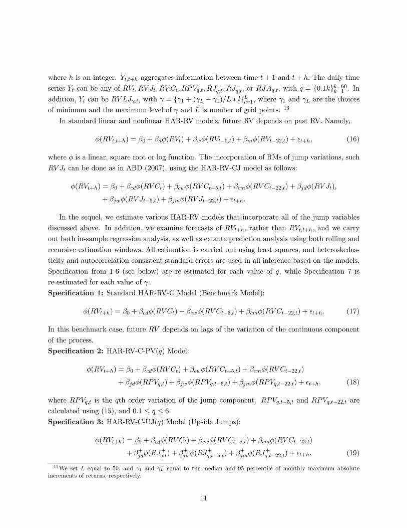
In standard linear and nonlinear HAR-RV models, future RV depends on past RV. Namely,

(+) = 0 + () + (−5) + (−22) + +, (16)

where is a linear, square root or log function. The incorporation of RMs of jump variations, such

can be done as in ABD (2007), using the HAR-RV-CJ model as follows:

(+) = 0 + ( ) + ( −5) + ( −22) + ( )

+ ( −5) + ( −22) + +

In the sequel, we estimate various HAR-RV models that incorporate all of the jump variables

discussed above. In addition, we examine forecasts of + rather than +, and we carry

out both in-sample regression analysis, as well as ex ante prediction analysis using both rolling and

recursive estimation windows All estimation is carried out using least squares, and heteroskedas-

ticity and autocorrelation consistent standard errors are used in all inference based on the models.

Specification from 1-6 (see below) are re-estimated for each value of while Specification 7 is

re-estimated for each value of .

Specification 1: Standard HAR-RV-C Model (Benchmark Model):

(+) = 0 + ( ) + ( −5) + ( −22) + + (17)

In this benchmark case, future depends on lags of the variation of the continuous component

of the process.

Specification 2: HAR-RV-C-PV() Model:

(+) = 0 + ( ) + ( −5) + ( −22)

+ () + (−5) + (−22) + + (18)

where is the th order variation of the jump component. −5 and −22 arecalculated using (15), and 01 ≤ ≤ 6Specification 3: HAR-RV-C-UJ() Model (Upside Jumps):

(+) = 0 + ( ) + ( −5) + ( −22)

+ +(+) + +(

+−5) + +(

+−22) + + (19)

13We set equal to 50, and 1 and equal to the median and 95 percentile of monthly maximum absolute

increments of returns, respectively.

11

+ +−5

+−22 measure the th order power variation of positive jumps today, last week,

and last month, and are calculated using (15), and 21 ≤ ≤ 6Specification 4: HAR-RV-C-DJ() Model (Downside Jumps):

(+) = 0 + ( ) + ( −5) + ( −22)

+ −(−) + −(

−−5) + −(

−−22) + + (20)

The range of is 21 ≤ ≤ 6Specification 5: HAR-RV-C-UDJ() Model (Upside and Downside Jumps):

(+) = 0 + ( ) + ( −5) + ( −22)

+ +(+) + +(

+−5) + +(

+−22)

+ −(−) + −(

−−5) + −(

−−22) + + (21)

Specification 6: HAR-RV-C-APJ() Model (Asymmetric Jumps):

(+) = 0 + ( ) + ( −5) + ( −22)

+ () + (−5) + (−22) + + (22)

This model uses RMs of signed jump power variations, i.e., measures of jump asymmetry, as

explanatory variables. These variables, −5 and −22 are calculated using(15).

Specification 7: HAR-RV-C-LJ() Model (Truncated Large Jumps):

(+) = 0 + ( ) + ( −5) + ( −22)

+ ( ) + ( −5) + ( −22) + + (23)

The forecast horizons that we examine are = 1 5 22 which correspond to one day, one week,

and one month ahead, respectively. For each specification (except for Specifications 1, 2 and 7),

there are 40 variants, corresponding to 40 different values of For specification 2, there are 60 vari-

ants and there are 50 variants for specification 7. In our forecasting experiments, the entire sample

of observations is divided into two samples, the estimation sample containing observations,

and the prediction sample containing = − (minus ) observations. Both rolling and recursivewindows of data are used in model estimation, prior to the construction of each new prediction. In

addition to reporting out-of-sample 2 statistics, calculated by projecting RV forecasts on historical

RV, we also report traditional in-sample adjusted 2 statistics calculated the using entire sample

of observations. In our prediction experiments, we also carry out pairwise Diebold and Mariano

(DM: 1995) predictive accuracy tests. Our DM tests assume quadratic loss, have a null of equal

predictive ability, and are asymptotically normally distributed (under a nonnestedness assumption

- see Corradi and Swanson (2006) and the references cited therein for a complete discussion). The

12

test statistic is = −1P

=1 (b) where = b21+ − b22+the bs are forecast errors fromthe two competing models, and b is a heteroskedasticity and autocorrelation consistent estimatorof the standard error of the mean of .

5 Empirical Findings

5.1 Data Description

S&P500 futures index and Dow 30 individual stock datasets (collected for the period 1993-2009

and 1993-2008, respectively) were obtained from the TAQ database. When processing the data, we

followed the common practice of eliminating from the sample those days with infrequent trades (less

than 60 transactions at our 5 minute frequency). In the literature, two methods are often applied

for filtering out an evenly-spaced sample - the previous tick method and the interpolation method

(Dacorogna, Gencay, Müller, Olsen, and Pictet (2001)). As shown in Hansen and Lund (2006), in

applications using quadratic variation, the interpolation method should not be used, as it leads to

realized volatilities with value 0 (see Lemma 3 in their paper). Therefore, we use the previous tick

method (i.e. choosing the last price observed during a given interval). We restrict our dataset to

regular time and ignore ad hoc transactions outside of this time interval. To reduce microstructure

noise effects, the suggested sampling frequency in the literature ranges from 5 minutes to 30 minutes.

We choose the 5 minute frequency, yielding 78 observations per day in most cases.14

5.2 Contribution of Jumps to Realized Volatility

All daily statistics are calculated using the formulae in Sections 2 with

∆ =1

=

1

# of 5 minute transactions / day

For instance, ∆ = 178 for most of the stocks in the sample. This implies that the time interval

[0 1] maps into a beginning time of 9 am (set equal to 0) and an end time of 4:30 pm (set equal

to 1), in our setup In all calculations involving integrated volatility and integrated quarticity, we

use multipower variation, as discussed above. Let denote the number of days in the sample. We

construct the time series {()}=1 andn

o=1

The average relative

contribution of continuous, jump, and large jump components to the variation of the process is

reported using the mean of the sample (i.e., we report the means of

and

)15 In this context, an important step is the choice truncation level, . If we choose arbitrarily large

truncation levels, then clearly we will find no evidence of large jumps. Also, one might imagine

14A main drawback of realized measures constructed using high frequency data is that they are contaminated by

mictrostructure noise, and hence our use of a 5 minute data interval. See Aït-Sahalia, Mykland and Zhang (2005)

for further dicussion.15 In the sequel, we provide numerical results for S&P500 futures, in cases were brevity becomes and issue, and

where qualitative findings remain the same. Complete results are available upon request.

13

proceeding by picking truncation levels based on the percentiles of the entire historical sample of

5 minute returns. However, results will then be difficult to interpret, as the usual choice of 90

percentiles leads to virtually no large jumps while the choice of 10 percentiles leads to a very

large number of large jumps. In addition, large jumps are often thought of as abnormal events that

arise at a frequency of one in several months or even years. Therefore, a reasonable way to proceed

is to pick the truncation level on the basis of the sample of the monthly maximal increments,

i.e., monthly abnormal events. Specifically, we set four levels = 1 2 3 4 to be the 50 75

90 and 95 percentiles of the entire sample of maximal increments from 1993-2009 for S&P500

futures and from 1993-2008 for the Dow 30 components. This is done in order to construct the

summary statistics reported in Table 1; while grid search based results are discussed in a subsequent

section. In particular, Table 1 summarizes average percentage of daily variation of the continuous

and jump components, at truncation levels 1 2 3 4 relative to daily realized variances, for the

sample period from 1993-2009, across jump pre-test significance levels, = 00001, 0001 0005

and 001. For example, at the = 0001 and 00001 levels, the average daily jump variations are

25.3% and 14.4% during the 1993-2009 period, respectively. Corresponding average variations of

large daily jumps at truncation level 3 are 1.7% and 0.8% respectively. This evidence is consistent

with previous evidence reported in the literature and discussed above regarding the clear prevalence

of jumps in financial data. For example, using the Dow 30 components examined in this paper,

Duong and Swanson (2011) find clear evidence of jumps.

5.3 RV Prediction using Realized Jump Power Variations and Realized Trun-

cated Large Jump Variations

We begin by calculating all daily RMs, as discussed above, using our S&P500 dataset; yielding

time series with = 4123 observations. In our out-of-sample forecasting experiments, we set

= 410.16 The models used in our experiments are discussed above and summarized in Section

3. Finally, as a point of reference, recall that the empirical analyses of exchange rates, equity

index returns, and bond yields reported in ABD (2007) suggest that the volatility jump component

is both highly important and distinctly less persistent than the continuous component, and that

separating "rough" jump movements from smooth continuous movements results in significant in-

sample volatility forecast improvements (i.e., linear and nonlinear HAR-RV-CJ models perform

better than models without "separate" jumps). In this section, we first discuss Specifications-6

outlined in Section 4. Specification 7 is thereafter discussed.

Consider S&P500 futures. Predictive performance is measured by both in-sample and out-of

sample 2 which is similar to approach taken in ABD (2007). We also carry out DM (1995)

predictive accuracy tests to determine whether the choice of matters when forecasting RV. Table

2 reports regression estimates, as well as in-sample and out-of-sample 2 values for linear, square

16We also analyzed alternative out-of-sample periods, including ={210, 310, 510, 610,710}. Results were quali-

tatively similar to those reported here, and are available upon request.

14

root and log HAR-RV-C models at daily ( = 1), weekly ( = 5) and monthly ( = 22) prediction

horizons. Entries in brackets are robust -statistics. When comparing in-sample and out-of-sample

2 statistics, it is clear that the square root and log models perform much better than their linear

counterparts, regardless of prediction horizon. For instance, for = 1 the in-sample and out-of-

sample 2 statistics for square root models are 0.45 and 0.34 while those of their linear counterparts

are 0.35 and 0.24, respectively. In addition, the estimates of , , as well as associated

-statistics confirm the long memory (persistence) property of volatility. For the linear model with

= 1 the -statistic associated with is 781 implying that the continuous component from the

previous month is potentially important for one-day ahead prediction of volatility. This statistical

pattern holds for square root and log models, across all forecast horizons. In addition, at prediction

horizon = 22 while the in-sample 2s are large, out-of sample results show deteriorating behavior,

as might be expected.

When constructing, +,

−, and, values of including {21 22 58 59 60}

were tried.17 Larger values of effectively eliminate the effects of the continuous component and of

smaller jumps, while magnifying the relevance of large jumps. In Tables 3A-3C, we report results

only for = 25 and = 5, as these are two good representative cases when distinguishing between

small and large jump power variations. Each table contains results of the jump coefficient esti-

mates and in- and out-sample 2 for linear, square root and log models.18 All bracketed entries

are -statistics. Observe first that jump coefficients are not usually statistically significant for = 5

(large jumps). This result holds across all model specifications, and holds for all cases where = 5.

For = 25, -statistics are significant for in linear and square root HAR-RV-C-PV() models.

For instance, the -statistics are 2.24 for = 1 and 1.98 for = 22 in linear models, respectively.

Turning to our "full decomposition" HAR-RV-C-UDJ() model reported in Table 3B, note that

the -statistic associated with − is 2.14, for = 22 in linear models.19 Upward jump variations

generally have a negligible impact in our prediction models, however. Most interestingly, correla-

tion between past and future is rather strong across all forecast horizons (daily, weekly

and monthly) for linear and square root models, as indicated by a large number of statistically

significant coefficient estimates on this variable (see Table 3C).

Table 4A summarizes results of tests carried out to compare the predictive accuracy of a subset

of our prediction models. In particular, and for each model listed in the first column of the table,

denotes the value of that yields the largest out-of-sample 2 values while denotes the value of

that yields the smallest 2 values, for = {25 + ∗ 01}=35=0 . The DM statistics in the first row

17For 6, prediction results are qualitatively the same as when = 6 and are therefore not discussed.18Table 2 already confirms the predictive performance of the realized measures of the continuous component. For

brevity, we thus exclude and further presentation of parameter estimates associated with continuous components.

Complete results are available upon request.19For brevity, we do not include a table for the HAR-RV-C-DJ () specification. Our experiments showed, however,

that downward jump variations have an impact on our predictions for the case = 25 across all forecast horizons.

For instance, for square root model, −statistics associated with are 2.10 for = 1 and = 22 respectively

while −statistic associated with is 252 for = 5

15

of each panel of the table are based on the comparison of each pair of ( ) models, and positive

values indicate that the model dominates, in terms of out-of-sample mean square forecast error

fit. Since almost all DM statistics are statistically significant and positive, we have evidence that

the highest out-of-sample 2 model is statistically superior to the lowest. Moreover, as we generally

see that = 25, we have strong evidence that large, seemingly rare and possibly jumps do not

help in prediction, while smaller, less rare and possibly serially correlated jumps do help.

Continuing our discussion of predictive performance, note that our prediction experiments show

improvements, both in- and out-of-sample, when RMs of jump power variations are used as addi-

tional predictors in volatility forecasting. For example, at forecast horizons = 1 and = 5, the

out-of sample 2 values of the benchmark HAR-RV-C square root models are 0.34 for = 1 and

0.24 for = 5 Compare these values with those of 0.37 and 0.26, which obtain when our HAR-

RV-C-PV() model is used to construct forecasts. This is equivalent to an 8% and 7.5% increase in

2 when switching from HAR-RV-C to HAR-RV-C-PV models. However, as shown in the table,

the continuous component, dominates in all prediction experiments, which is consistent with

previous findings in the literature on volatility forecasting using high frequency data. Moreover,

there is little improvements in 2 when HAR-RV-C-UDJ() is used for prediction. Interestingly,

results in the table suggest that in- and out-of sample 2 values are smaller, the larger is (com-

pare the cases where = 25 and = 5). This pattern is clearly depicted in the figures discussed

below.20

Finally, the above conclusions are confirmed in Figures 1, 2, and 4. In these figures, both in-

and out-of-sample 2 values are reported. In all plots, the vertical axis ranges from 0 to 1 and

denotes the value 2. The horizontal axis ranges from 0.1 to 6, representing 60 grid points of values

of , i.e. = {0 + 01 ∗ }60=1.Notice first that there is little to choose between the models, in a majority of cases, confirming

our earlier finding that jumps, while prevalent, add relatively little to predictive accuracy.

Second, comparing "no jump test" cases with "jump test" cases indicates that findings do

change, to some degree, when jump pre-tests are used in the construction of jump variation vari-

ables. In particular, compare Figures 1A and 1B (the case where S&P500 futures are modelled).

The maximal out-of-sample 2 values that are achieved when no jump tests are used are usually

modestly higher, for linear and square root models. Naturally, the 2−"best" value of also varies,although to a very small extent, when comparing these two figures. The same broad result holds

when comparing in-sample 2 values. For illustration, we present the in-sample prediction results

for S&P500 futures when jump tests are used in Figure 2. In summary, little is gained in our exper-

iments by constructing realized measures that directly incorporate a variable indicating whether

our jump test find evidence of jumps during a particular day.

Third, Figures 2 and 4 clearly indicates that the 2−"best" value of is higher when S&P50020Note that our figures only summarize linear and square root models. Qualitatively similar figures for log models

are available upon request.

16

index returns are predicted, than when individual DOW components are predicted (see Figure

4). This suggests that aggregation plays a crucial role in risk prediction. Values of less than 2

dominate under individual stocks, while values greater than 2 dominate under our index variable

as shown in Figure 2. Evidently, jumps matter much more for risk prediction in a return variable

that aggregates many jumps from many companies than in isolated companies. Finally, while the

in-sample 2−"best" value of is always far less than 2 for square root models, when evaluatingthe S&P500 index (see Figures 2), the out—of-sample 2−"best" value of is always far greaterthan 2 when jump tests are used (see Figures 1B). This rather interesting finding suggests that

what’s best for in-sample analysis is far from best for out-of-sample analysis. In particular, jumps

do play a role, at least when modelling aggregate (index) data such as S&P500 futures returns; and

while modelling jump risk power variations may not be important for in-sample fit, it clearly plays

an important role in out-of-sample volatility prediction.

In closing, we turn to the HAR-RV-C-LJ () model (Specification 7). The motivation for the

examination of this specification is twofold. First, we use the prediction results of HAR-RV-C-LJ ()

as a robustness check of our finding that "large" jumps help less for prediction than "small" jumps

in the prediction of future RV. Second, as discussed in Section 3, though the construction of large

jump variations by the jump decomposition approach is intuitively interesting, the implementation

of this method is not straightforward due to the fact that is arbitrarily chosen. Our approach is

to simply carry out a grid search across , in order to ascertain the threshold yielding the largest

out-of-sample 2, for S&P500 futures and a sample of Dow 30 components. For our application,

we set = [1 50] and we set the number of grid points to be 50 where 1 and 50 correspond to

the median and 95th percentiles of the monthly maximum absolute increments of S&P500 futures

returns (or Dow 30 component returns).21 Similar to the RV prediction using the HAR-RV-C-PV()

model, we re-estimated the HAR-RV-C-LJ () model for = {1 (50 − 1)50 ∗ }50=1 and carriedout forecasting experiments. Table 3D reports estimation results for two representative cases (i.e.,

small ( = 20) and large ( = 40) jump variations) for S&P500 futures returns. T- statistics are

significant for both = 20 and = 40, suggesting that jumps matter. However, both in- and

out-of-sample 2 values are marginally higher for = 20. These results are confirmed in Table 4B,

where DM predictive accuracy tests are reported, since the DM statistics indicate test rejection.

In this table, and denote the values of grid point that yield the largest and smallest 2,

respectively, for = {1 2 50}. In many cases, is close to 1 while is close to 50. Thus, wehave further evidence that larger jumps help less in the prediction of future volatility. Figures 3 and

5 contain plots of out-of sample 2 statistics for S&P500 futures as well as selected components

of Dow 30 based on the HAR-RV-C-LJ () model. In these figures, 2 appears on the vertical

axis, while the horizontal axis has values ranging from 1 to 50, representing the 50 grid pointsi.e.

{1 (50 − 1)50 ∗ }50=1. Though the changes are marginal, all the figures share a similar pattern21We also experimented with various other intervals chosen on the basis of different return percentiles. The choice

of median and 95th percentiles is reported for illustrative purposes.

17

in which 2-values are monotonically decreasing as the truncation level, increases. This again

points to a conclusion that larger jumps help less in the prediction of future RV than smaller jumps.

6 Concluding Remarks

In this paper, we examine jump power variations and truncated large jump variations in the context

of volatility forecasting. Our key findings can be summarized as follows. First, we find evidence

that jumps characterize the structure of S&P500 futures and the individual stocks that we examine.

Second, our prediction experiments show improvements, both in- and out-of-sample, when RMs of

jump power variations are used as additional predictors in volatility forecasting. However, past

"large" jump power variations help less in the prediction of future realized volatility, than past

"small" jump power variations. Third, the continuous component dominates in all prediction

experiments, which is consistent with previous findings in the literature on volatility forecasting

using high frequency data. Fourth, incorporation of downside and upside jump power variations

does improve predictability, albeit to a limited extent. Fifth, comparing jump measures constructed

with no pre-jump test with those constructed using a jump pre-test indicates that findings do

change, to some degree, when jump tests are used in the construction of jump variation variables.

Additionally, the power of associated with our 2−"best" model is higher when S&P500 indexreturns are predicted, than when individual DOW components are predicted. This suggests that

aggregation plays a role in risk prediction. Values of less than 2 dominate for individual stocks,

while values greater than 2 dominate for our index variable. Taken together, these results suggest

that what’s best for in-sample analysis is far from best for out-of-sample analysis. Finally, empirical

analysis on the predictive content of the RMs of truncated large jump variations is consistent with

the above finding that large jumps help less than small jumps.

Many questions remain for future research. For example, the empirical findings in this paper

are based on theoretical results that do not take into account microstructure noise. A next natural

step would be to examine microstructure noise robust estimators of jump power variations such

as those developed in Li (2013) using ultra high frequency data (see also Fan and Wang (2008),

Jacod, Podolskij and Vetter (2010), and Zu and Boswik (2014)).22 In this case, predictive perfor-

mance measures would need to be corrected to incorporate microstructure noise effects. (see Asai,

McAleer, and Medeiros (2012) for an interesting discussion of modelling and forecasting noisy re-

alized volatility). Additionally, it remains to be seen whether prediction based "gains" associated

with modelling jumps translate into improved performance when carrying out real-world derivative

pricing, asset allocation, and hedging exercises.

22Note that many papers in the literature on RV prediction use "standard" 5-minute data, which has been shown by

Aït-Sahalia, Mykland, and Zhang (2005) to be the "optimal" frequency for mitigating the impact of microstructure

noise. Also, there is very limited evidence on the predictive superiority of a particular frequency versus the other. For

example, an empirical analysis by Liu, Patton, and Sheppard (2012) shows that it is difficult for other complicated

realized measures of volatility using different frequencies to beat 5-minute RV.

18

ReferencesAït-Sahalia, Y. (2002). Telling from discrete data whether the underlying continuous-time

model is a diffusion. Journal of Finance 57, 2075-2112.

Aït-Sahalia, Y. and Jacod, J. (2009a). Testing for Jumps in a Discretely Observed Process.

Annals of Statistics 37, 184-222.

Aït-Sahalia, Y. and Jacod, J. (2009b). Estimating the Degree of Activity of Jumps in High

Frequency Data. Annals of Statistics 37, 2202-2244.

Aït-Sahalia, Y. and Jacod, J. (2012). Analyzing the Spectrum of Asset Returns: Jump and

Volatility Components in High Frequency Data. Journal of Economic Literature 50, 1007-1050.

Aït-Sahalia, Y., Mykland, P. A., and Zhang, L. (2005). How Often to Sample a Continuous-

Time Process in the Presence of Market Microstructure Noise. Review of Financial Studies 18,

351-416.

Andersen, T. G., Bollerslev, T., and Diebold, F. X. (2007). Roughing it Up: Including Jump

Components in the Measurement, Modeling and Forecasting of Return Volatility. Review of Eco-

nomics and Statistics 89, 701-720.

Andersen, T. G., Bollerslev, T., Diebold, F.X. and Labys, P. (2001). The Distribution of

Exchange Rate Volatility. Journal of the American Statistical Association 96, 42-55. Correction

Published in 2003, volume 98, page 501.

Andersen, T.G., Bollerslev, T., Diebold, F.X. and Labys, P. (2003). Modelling and Forecasting

Realized Volatility. Econometrica 71, 579-626.

Ang, A., Chen, J., and Xing, Y. (2006). Downside Risk. Review of Financial Studies 19,

1191-1239.

Asai, M., McAleer, M. and Medeiros M. (2012). “Modelling and Forecasting Daily Volatility

with Noisy Realized Volatility Measures”. Computational Statistics & Data Analysis, 56, 217-230.

Barndorff-Nielsen, O.E., Shephard, N. (2004). Power and Bipower Variation with Stochastic

Volatility and Jumps (with discussion). Journal of Financial Econometrics 2, 1-48.

Barndorff-Nielsen, O.E., Shephard, N. (2006). Econometrics of Testing for Jumps in Financial

Economics using Bipower Variation. Journal of Financial Econometrics 4, 1-30.

Barndorff-Nielsen, O.E., Hansen, P.R., Lunde A. and Shephard, N. (2008). Designing Realized

Kernels to Measure the Ex-Post Variation of Equity Prices in the Presence of Noise. Econometrica

76, 1481-1536.

Barndorff-Nielsen O.E., Kinnebrock, S. and Shephard, N. (2010). Measuring downside risk -

realised semivariance,” in Volatility and Time Series Econometrics: Essays in Honor of Robert F.

Engle, ed. by Bollerslev, T., Russell, J. and Watson, M. Oxford University Press.

Carr, P., Geman, H., Madan, D.B., Yor, M., (2002). The Fine Structure of Asset Returns: An

Empirical Investigation. Journal of Business 75, 305-332.

Cont, R. and Mancini, C. (2007). Nonparametric Tests for Analyzing the Fine Structure of

19

Price Fluctuations. Working Paper, Columbia University Center for Financial Engineering.

Corradi, V. and Swanson N.R. (2006). Predictive Density Evaluation. Printed in Clive W.J.

Granger, Graham Elliot and Allan Timmerman. Handbook of Economic Forecasting, Elsevier,

Amsterdam, 197-284.

Corradi, V., Distaso, W. and Swanson N.R. (2009). Predictive Density Estimators for Daily

Volatility Based on the Use of Realized Measures. Journal of Econometrics 150, 119-138.

Corradi, V., Distaso, W. and Swanson N.R. (2011). Predictive Infererence for Integrated Volatil-

ity. Journal of the American Statistical Association 106, 1496-1512.

Corsi, F. (2004). A Simple Long Memory Model of Realized Volatility. Working Paper, Uni-

versity of Southern Switzerland.

Corsi, F., Pirino, D., Reno, R. (2008). Volatility Forecasting: The Jumps Do Matter. SSRN

Working Paper.

Dacorogna, M.M., Gencay, R., Müller, U., Olsen, R.B., and Pictet, O.B. (2001). An Intro-

duction to High-Frequency Finance. Academic Press: London.

Diebold, F. X. and Mariano, R. S. (1995). Comparing Predictive Accuracy. Journal of Business

and Economic Statistics 13(3), 253-63.

Ding, Z., C. Granger, and Engle, R. (1993). A Long Memory Property of Stock Market Returns

and a New Model. Journal of Empirical Finance 1, 83-106.

Ding, Z. and Granger, C. W. J. (1996). Modeling Volatility Persistence of Speculative Returns:

A New Approach. Journal of Econometrics 73, 185-215.

Duong, D. and Swanson, N.R. (2011). Volatility in Discrete and Continuous Time Models:

A Survey with New Evidence on Large and Small Jumps, Missing Data Methods: Advances in

Econometrics 27, 179-233.

Fan, J. and Wang, Y. (2008). Spot Volatility Estimation for High-Frequency Data. Statistics

and Its Interface 1, 279—288.

Ghysels, E. and Sohn, B. (2009). Which Power Variation Predicts Volatility Well ? Journal of

Empirical Finance, 16, 686-700.

Granger, C.W. J. (2008). In Praise of Pragmatic Econometrics. In J. L. Castle and N. Shephard

(Eds.), The Methodology and Practice of Econometrics: A Festschrift in honour of David F Hendry,

105-116. Oxford University Press.

Hansen, P.R. and Lunde, A. (2006). Realized Variance and Market Microstructure noise (with

comments and rejoinder). Journal of Business and Economic Statistics 24, 127-218.

Huang, X. and Tauchen, G. (2005). The Relative Contribution of Jumps to Total Price Variance.

Journal of Financial Econometrics 3, 456-499.

Jacod J. (2008), Asymptotic Properties of Realized Power Variations and Related Functionals

of Semimartingales. Stochastic Processes and Their Applications 118, 517-559.

Jacod, J., Podolskij, M. and Vetter, M. (2010), Limit Theorems for Moving Averages of Dis-

20

cretized Processes Plus Noise, Annals of Statistics 38, 1478-1545.

Jiang, G. J. and Oomen, R.C.A. (2008). Testing for Jumps when Asset Prices are Observed

with Noise - A "Swap Variance" Approach. Journal of Econometrics 144, 352-370.

Lee, S. and Mykland, P. A. (2008). Jumps in Financial Markets: A New Nonparametric Test

and Jump Clustering. Review of Financial Studies 21, 2535-2563.

Li, Jia (2013). Robust Estimation and Inference for Jumps in Noisy High Frequency Data: a

Local-to-Continuity Theory for the Pre-averaging Method. Econometrica 81, 1673-1693.

Liu, C. and Maheu, M.J. (2005). Modeling and Forecasting Realized Volatility: The Role of

Power Variation. Working Paper, University of Toronto.

Liu, L., Patton, A.J. and Sheppard, K. (2012). Does Anything Beat 5-Minute RV? A Compar-

ison of Realized Measures Across Multiple Asset Classes. Working Paper, Duke University.

Maheu, J. M., and McCurdy, T. H. (2004). News Arrival, Jump Dynamics and Volatility

Components for Individual Stock Returns. Journal of Finance 59, 755-793.

Müller, U. A., Dacorogna, M.M., Davé, R.D., Olsen, R.B., Pictet, O.V. and von Weizsäcker, J.

E. (1997). Volatilities of Different Time Resolutions - Analyzing the Dynamics of Market Compo-

nents. Journal of Empirical Finance 4, 213-239.

Perez-Quiros, G., and Timmermann, A. (2001). Business Cycle Asymmetries in Stock Returns:

Evidence from Higher Order Moments and Conditional Densities. Journal of Econometrics 103,

259-306.

Patton, A. and Shephard, K. (2011). Good Volatility, Bad Volatility: Signed Jumps and Per-

sistence of Volatility. Working Paper, Duke University.

Timmermann, A. (2000). Moments of Markov Switching models. Journal of Econometrics 96,

75-111.

Todorov, V. and Tauchen, G. (2010). Activity Signature Functions with Application for High-

Frequency Data Analysis. Journal of Econometrics 154, 125-138.

Zhang, L. (2006). Efficient Estimation of Stochastic Volatility Using Noisy Observations: A

Multi-Scale Approach. Bernoulli 12, 1019-1043.

Zu, Y. and Boswijk, H.P. (2014). Estimating SPot Volatility with High -Frequency Data.

Journal of Econometrics 181, 117-135.

21

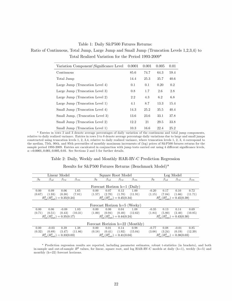
Table 1: Daily S&P500 Futures Returns:

Ratio of Continuous, Total Jump, Large Jump and Small Jump (Truncation Levels 1,2,3,4) to

Total Realized Variation for the Period 1993-2009*

Variation Component\Significance Level 0.0001 0.001 0.005 0.01

Continuous 85.6 74.7 64.3 59.4

Total Jump 14.4 25.3 35.7 40.6

Large Jump (Truncation Level 4) 0.1 0.1 0.20 0.2




Small Jump (Truncation Level 4) 14.3 25.2 35.5 40.4

Small Jump, (Truncation Level 3) 13.6 23.6 33.1 37.8

Small Jump (Truncation Level 2) 12.2 21 29.5 33.8

Small Jump (Truncation Level 1) 10.3 16.6 22.4 25.2∗ Entries in rows 2 and 3 denote average percentages of daily variation of the continuous and total jump components,

relative to daily realized variance. Entries in rows 3 to 8 denote average percentage daily variations due to large and small jumps

constructed using truncation levels 1, 2, 3,4, relative to daily realized variance, where truncation levels 1, 2, 3, 4 correspond to

the median, 75th, 90th, and 95th percentiles of monthly maximum increments of (log) prices of S&P500 futures returns for the

sample period 1993-2009. Entries are caculcated in conjunction with jump tests carried out using 4 different significance levels,

=00001 0001 0005 001. See Sections 2 and 5 for further details.

Table 2: Daily, Weekly and Monthly HAR-RV-C Prediction Regression

Results for S&P500 Futures Returns (Benchmark Model)*

Linear Model Square Root Model Log Model0 0 0

Forecast Horizon h=1 (Daily)0.00 0.09 0.06 1.65 0.00 0.07 0.12 1.00 -0.20 0.17 0.10 0.72

(0.67) (1.93) (0.38) (7.81) (1.57) (2.70) (1.70) (11.91) (1.15) (7.04) (1.66) (11.71)

2(2) = 035(024) 2(

2) = 045(034) 2(

2) = 045(039)

Forecast Horizon h=5 (Weeky)0.00 0.06 -0.08 1.83 0.00 0.06 0.04 1.08 -0.35 0.13 0.14 0.69

(0.71) (0.51) (0.43) (10.31) (1.00) (0.94) (0.40) (12.62) (1.84) (5.80) (2.40) (10.85)

2(2) = 035(017) 2(

2) = 044(024) 2(

2) = 043(030)

Forecast Horizion h=22 (Monthly)0.00 -0.03 0.39 1.38 0.00 0.01 0.14 0.98 -0.77 0.08 -0.01 0.85

(0.32) (0.89) (3.47) (11.86) (0.18) (0.41) (1.92) (15.04) (3.08) (3.24) (0.19) (12.39)

2(2) = 033(003) 2(

2) = 041(004) 2(

2) = 038(003)

∗ Prediction regression results are reported, including parameter estimates, robust t-statistics (in brackets), and bothin-sample and out-of-sample 2 values, for linear, square root, and log HAR-RV-C models at daily (h=1), weekly (h=5) and

monthly (h=22) forecast horizons.

22

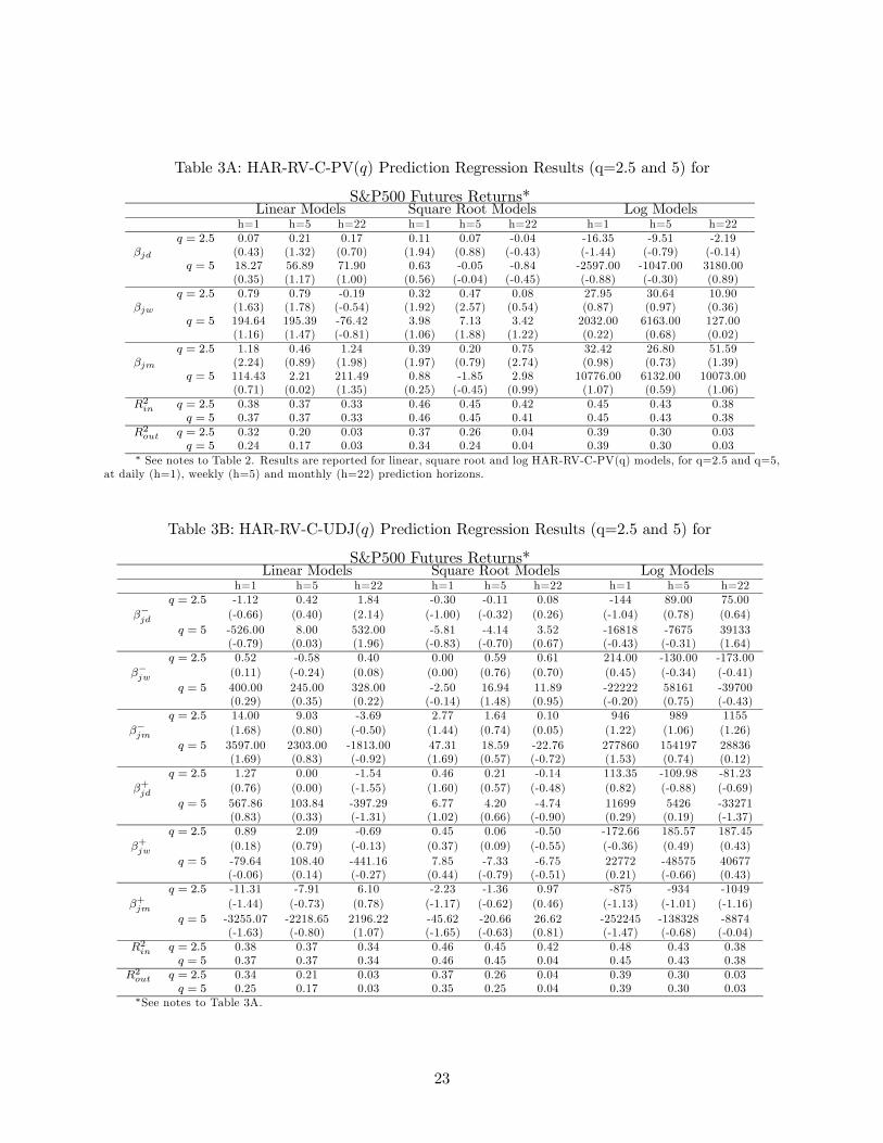
Table 3A: HAR-RV-C-PV() Prediction Regression Results (q=2.5 and 5) for

S&P500 Futures Returns*Linear Models Square Root Models Log Models

h=1 h=5 h=22 h=1 h=5 h=22 h=1 h=5 h=22

= 25 0.07 0.21 0.17 0.11 0.07 -0.04 -16.35 -9.51 -2.19

(0.43) (1.32) (0.70) (1.94) (0.88) (-0.43) (-1.44) (-0.79) (-0.14)

= 5 18.27 56.89 71.90 0.63 -0.05 -0.84 -2597.00 -1047.00 3180.00

(0.35) (1.17) (1.00) (0.56) (-0.04) (-0.45) (-0.88) (-0.30) (0.89)

= 25 0.79 0.79 -0.19 0.32 0.47 0.08 27.95 30.64 10.90

(1.63) (1.78) (-0.54) (1.92) (2.57) (0.54) (0.87) (0.97) (0.36)

= 5 194.64 195.39 -76.42 3.98 7.13 3.42 2032.00 6163.00 127.00

(1.16) (1.47) (-0.81) (1.06) (1.88) (1.22) (0.22) (0.68) (0.02)

= 25 1.18 0.46 1.24 0.39 0.20 0.75 32.42 26.80 51.59

(2.24) (0.89) (1.98) (1.97) (0.79) (2.74) (0.98) (0.73) (1.39)

= 5 114.43 2.21 211.49 0.88 -1.85 2.98 10776.00 6132.00 10073.00

(0.71) (0.02) (1.35) (0.25) (-0.45) (0.99) (1.07) (0.59) (1.06)

2 = 25 0.38 0.37 0.33 0.46 0.45 0.42 0.45 0.43 0.38

= 5 0.37 0.37 0.33 0.46 0.45 0.41 0.45 0.43 0.38

2 = 25 0.32 0.20 0.03 0.37 0.26 0.04 0.39 0.30 0.03

= 5 0.24 0.17 0.03 0.34 0.24 0.04 0.39 0.30 0.03∗ See notes to Table 2. Results are reported for linear, square root and log HAR-RV-C-PV(q) models, for q=2.5 and q=5,

at daily (h=1), weekly (h=5) and monthly (h=22) prediction horizons.

Table 3B: HAR-RV-C-UDJ() Prediction Regression Results (q=2.5 and 5) for


h=1 h=5 h=22 h=1 h=5 h=22 h=1 h=5 h=22

= 25 -1.12 0.42 1.84 -0.30 -0.11 0.08 -144 89.00 75.00

−

(-0.66) (0.40) (2.14) (-1.00) (-0.32) (0.26) (-1.04) (0.78) (0.64)

= 5 -526.00 8.00 532.00 -5.81 -4.14 3.52 -16818 -7675 39133

(-0.79) (0.03) (1.96) (-0.83) (-0.70) (0.67) (-0.43) (-0.31) (1.64)

= 25 0.52 -0.58 0.40 0.00 0.59 0.61 214.00 -130.00 -173.00

− (0.11) (-0.24) (0.08) (0.00) (0.76) (0.70) (0.45) (-0.34) (-0.41)

= 5 400.00 245.00 328.00 -2.50 16.94 11.89 -22222 58161 -39700

(0.29) (0.35) (0.22) (-0.14) (1.48) (0.95) (-0.20) (0.75) (-0.43)

= 25 14.00 9.03 -3.69 2.77 1.64 0.10 946 989 1155

− (1.68) (0.80) (-0.50) (1.44) (0.74) (0.05) (1.22) (1.06) (1.26)

= 5 3597.00 2303.00 -1813.00 47.31 18.59 -22.76 277860 154197 28836

(1.69) (0.83) (-0.92) (1.69) (0.57) (-0.72) (1.53) (0.74) (0.12)

= 25 1.27 0.00 -1.54 0.46 0.21 -0.14 113.35 -109.98 -81.23

+

(0.76) (0.00) (-1.55) (1.60) (0.57) (-0.48) (0.82) (-0.88) (-0.69)

= 5 567.86 103.84 -397.29 6.77 4.20 -4.74 11699 5426 -33271

(0.83) (0.33) (-1.31) (1.02) (0.66) (-0.90) (0.29) (0.19) (-1.37)

= 25 0.89 2.09 -0.69 0.45 0.06 -0.50 -172.66 185.57 187.45

+ (0.18) (0.79) (-0.13) (0.37) (0.09) (-0.55) (-0.36) (0.49) (0.43)

= 5 -79.64 108.40 -441.16 7.85 -7.33 -6.75 22772 -48575 40677

(-0.06) (0.14) (-0.27) (0.44) (-0.79) (-0.51) (0.21) (-0.66) (0.43)

= 25 -11.31 -7.91 6.10 -2.23 -1.36 0.97 -875 -934 -1049

+ (-1.44) (-0.73) (0.78) (-1.17) (-0.62) (0.46) (-1.13) (-1.01) (-1.16)

= 5 -3255.07 -2218.65 2196.22 -45.62 -20.66 26.62 -252245 -138328 -8874

(-1.63) (-0.80) (1.07) (-1.65) (-0.63) (0.81) (-1.47) (-0.68) (-0.04)

2 = 25 0.38 0.37 0.34 0.46 0.45 0.42 0.48 0.43 0.38

= 5 0.37 0.37 0.34 0.46 0.45 0.04 0.45 0.43 0.38

2 = 25 0.34 0.21 0.03 0.37 0.26 0.04 0.39 0.30 0.03

= 5 0.25 0.17 0.03 0.35 0.25 0.04 0.39 0.30 0.03∗See notes to Table 3A.

23

Table 3C: HAR-RV-C-APJ() Prediction Regression Results (q=2.5 and 5) for


h=1 h=5 h=22 h=1 h=5 h=22 h=1 h=5 h=22

= 25 0.07 0.21 0.17 0.08 0.05 -0.03 -16.14 -9.32 -2.04

(0.43) (1.32) (0.70) (1.97) (0.90) (-0.43) (-1.43) (-0.78) (-0.13)

= 5 18.27 56.89 71.90 0.45 0.00 -0.59 -2596.87 -1046.81 3180.15

(0.35) (1.17) (1.00) (0.57) (0.00) (-0.45) (-0.88) (-0.30) (0.89)

= 25 0.79 0.79 -0.19 0.23 0.33 0.06 27.70 30.42 10.64

(1.63) (1.78) (-0.54) (1.93) (2.59) (0.55) (0.87) (0.97) (0.36)

= 5 194.64 195.39 -76.42 2.94 4.93 2.42 2031.94 6162.49 127.11

(1.16) (1.47) (-0.81) (1.11) (1.90) (1.23) (0.22) (0.68) (0.02)

= 25 1.18 0.46 1.24 0.27 0.14 0.53 32.37 26.71 51.50

(2.24) (0.89) (1.98) (1.95) (0.81) (2.74) (0.99) (0.73) (1.39)

= 5 114.43 2.21 211.49 0.50 -1.22 2.10 10776.18 6131.78 10073.20

(0.71) (0.02) (1.35) (0.20) (-0.44) (0.99) (1.07) (0.59) (1.06)

2 = 25 0.38 0.37 0.34 0.46 0.45 0.42 0.45 0.43 0.38

= 5 0.37 0.37 0.34 0.46 0.45 0.42 0.45 0.43 0.38

2 = 25 0.32 0.20 0.03 0.37 0.26 0.04 0.39 0.30 0.03

= 5 0.24 0.17 0.03 0.34 0.24 0.04 0.39 0.30 0.03∗See notes to Table 3A.

Table 3D: HAR-RV-C-LJ() Prediction Regression Results ( = 20 and 40) for

S&P500 Futures Returns, with Jump Test*Linear Models Square Root Models Log Models

= 20 0.01 0.07 0.04 0.03 0.06 -0.02 1.37 5.94 1.40

(0.24) (1.34) (0.64) (1.23) (1.59) (-0.50) (0.44) (1.38) (0.26)

= 40 0.02 0.07 0.13 0.04 0.03 0.07 0.82 2.83 10.58

(0.30) (1.02) (1.39) (0.74) (0.51) (1.01) (0.24) (0.64) (2.16)

= 20 0.27 0.26 -0.06 0.14 0.11 0.03 10.55 20.04 -7.97

(1.98) (1.99) (-0.54) (2.75) (2.14) (0.62) (0.92) (2.26) (-0.80)

= 40 0.27 0.36 -0.20 0.12 0.23 -0.07 1.43 23.89 -18.55

(1.36) (2.26) (-1.94) (1.10) (2.77) (-0.89) (0.11) (2.86) (-2.28)

= 20 0.46 0.17 0.42 0.08 0.07 0.21 -40.41 -55.06 -18.16

(2.64) (0.95) (1.97) (1.34) (1.09) (2.55) (-0.81) (-1.01) (-0.34)

= 40 0.18 -0.13 0.19 0.01 -0.11 0.09 -17.43 -43.01 -12.85

(0.91) (-0.94) (0.91) (0.13) (-1.23) (0.98) (-0.59) (-1.34) (-0.38)

2 = 20 0.38 0.37 0.33 0.46 0.45 0.42 0.02 0.02 0.02

= 40 0.37 0.37 0.33 0.45 0.45 0.41 0.02 0.02 0.02

2 = 20 0.27 0.15 0.02 0.35 0.23 0.03 0.33 0.25 0.02

= 40 0.26 0.15 0.02 0.34 0.22 0.02 0.33 0.25 0.02∗ See notes to Table 3A. Results are reported for linear, square root and log HAR-RV-C-LJ() models, for two selected

truncation levels, = 20 and = 40, where = {1 + (50 − 1)50 ∗ }=50=1, where 1 and 50 correspond to the median

and to 95th percentile of monthly maximum increments of S&P500 futures returns. See Sections 4 and 5 for further details.

24

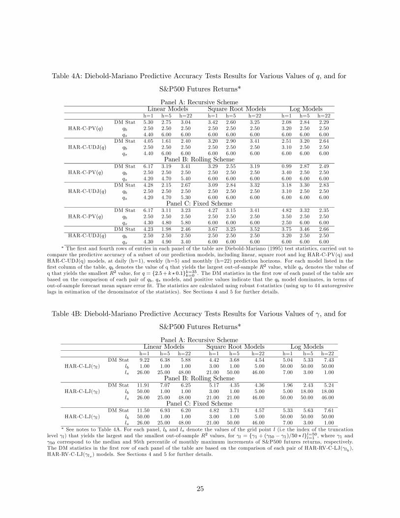
Table 4A: Diebold-Mariano Predictive Accuracy Tests Results for Various Values of and for

S&P500 Futures Returns*

Panel A: Recursive SchemeLinear Models Square Root Models Log Models

h=1 h=5 h=22 h=1 h=5 h=22 h=1 h=5 h=22

DM Stat 5.30 2.75 3.04 3.42 2.60 3.25 2.08 2.84 2.29

HAR-C-PV() 2.50 2.50 2.50 2.50 2.50 2.50 3.20 2.50 2.50

4.40 6.00 6.00 6.00 6.00 6.00 6.00 6.00 6.00

DM Stat 4.05 1.61 2.40 3.20 2.90 3.41 2.51 3.20 2.64

HAR-C-UDJ() 2.50 2.50 2.50 2.50 2.50 2.50 3.10 2.50 2.50

4.40 6.00 6.00 6.00 6.00 6.00 6.00 6.00 6.00

Panel B: Rolling SchemeDM Stat 6.17 3.19 3.41 3.29 2.55 3.19 0.99 2.87 2.49

HAR-C-PV() 2.50 2.50 2.50 2.50 2.50 2.50 3.40 2.50 2.50

4.20 4.70 5.40 6.00 6.00 6.00 6.00 6.00 6.00

DM Stat 4.28 2.15 2.67 3.09 2.84 3.32 3.18 3.30 2.83

HAR-C-UDJ() 2.50 2.50 2.50 2.50 2.50 2.50 3.10 2.50 2.50

4.20 4.70 5.30 6.00 6.00 6.00 6.00 6.00 6.00

Panel C: Fixed SchemeDM Stat 6.17 3.11 3.23 4.27 3.15 3.41 4.82 3.32 2.35

HAR-C-PV() 2.50 2.50 2.50 2.50 2.50 2.50 3.50 2.50 2.50

4.30 4.80 5.80 6.00 6.00 6.00 2.50 6.00 6.00

DM Stat 4.23 1.98 2.46 3.67 3.25 3.52 3.75 3.46 2.66

HAR-C-UDJ() 2.50 2.50 2.50 2.50 2.50 2.50 3.20 2.50 2.50

4.30 4.90 3.40 6.00 6.00 6.00 6.00 6.00 6.00∗ The first and fourth rows of entries in each panel of the table are Diebold-Mariano (1995) test statistics, carried out to

compare the predictive accuracy of a subset of our prediction models, including linear, square root and log HAR-C-PV(q) and

HAR-C-UDJ(q) models, at daily (h=1), weekly (h=5) and monthly (h=22) prediction horizons. For each model listed in the

first column of the table, denotes the value of q that yields the largest out-of-sample 2 value, while denotes the value of

q that yields the smallest 2 value, for = {25+ ∗ 01}=35=0 . The DM statistics in the first row of each panel of the table are

based on the comparison of each pair of , models, and positive values indicate that the model dominates, in terms of

out-of-sample forecast mean square error fit. The statistics are calculated using robust -statistics (using up to 44 autoregresive

lags in estimation of the denominator of the statistics). See Sections 4 and 5 for further details.

Table 4B: Diebold-Mariano Predictive Accuracy Tests Results for Various Values of and for

S&P500 Futures Returns*

Panel A: Recursive SchemeLinear Models Square Root Models Log Models

h=1 h=5 h=22 h=1 h=5 h=22 h=1 h=5 h=22

DM Stat 9.22 6.38 5.88 4.42 3.68 4.54 5.04 5.33 7.43

HAR-C-LJ() 1.00 1.00 1.00 3.00 1.00 5.00 50.00 50.00 50.00

26.00 25.00 48.00 21.00 50.00 46.00 7.00 3.00 1.00

Panel B: Rolling SchemeDM Stat 11.91 7.07 6.25 5.17 4.35 4.36 1.96 2.43 5.24

HAR-C-LJ() 50.00 1.00 1.00 3.00 1.00 5.00 5.00 18.00 18.00

26.00 25.00 48.00 21.00 21.00 46.00 50.00 50.00 46.00

Panel C: Fixed SchemeDM Stat 11.50 6.93 6.20 4.82 3.71 4.57 5.33 5.63 7.61

HAR-C-LJ() 50.00 1.00 1.00 3.00 1.00 5.00 50.00 50.00 50.00

26.00 25.00 48.00 21.00 50.00 46.00 7.00 3.00 1.00∗ See notes to Table 4A. For each panel, and denote the values of the grid point (i.e the index of the truncation

level ) that yields the largest and the smallest out-of-sample 2 values, for = {1 + (50 − 1)50 ∗ }=50=1

, where 1 and

50 correspond to the median and 95th percentile of monthly maximum increments of S&P500 futures returns, respectively.

The DM statistics in the first row of each panel of the table are based on the comparison of each pair of HAR-RV-C-LJ( ),

HAR-RV-C-LJ( ) models. See Sections 4 and 5 for further details.

25

Figure 1A: Out-of-sample 2 Values for S&P500 Futures for Jump Power Variation Models,

No Jump Test*

.08

.12

.16

.20

.24

.28

.32

.36

.40

1 2 3 4 5 6

Power q

HAR-RV-CHAR-RV-C-PVHAR-RV-C-UJHAR-RV-C-DJHAR-RV-C-UDJ

Linear Model and Forecast Horizon h=1

.08

.12

.16

.20

.24

.28

.32

.36

.40

1 2 3 4 5 6

Power q


Square Root Model and Forecast Horizon h=1

.08

.12

.16

.20

.24

.28

.32

.36

.40

1 2 3 4 5 6

Power q



.08

.12

.16

.20

.24

.28

.32

.36

.40

0.4 0.8 1.2 1.6 2.0 2.4 2.8 3.2 3.6 4.0

Power q



∗ The figure contains plots of out-of-sample 2 values for linear, square root HAR-RV-C, HAR-RV-C-PV(q), HAR-RV-C-UJ(q), HAR-RV-C-DJ(q), HAR-RV-C-UDJ(q) models at daily (h=1), weekly (h=5) and monthly (h=22) prediction horizons,

for the case where jumps tests are not used when calculating realized measures of jumps for S&P500 futures returns, for the

sample period 1993-2009. In each plot, the vertical axis contains entries ranging from 0 to 1. These are 2 statistic values.

Horizontal axis entries range from 0.1 to 6, representing 60 grid points of values of q, i.e. = {0 + 01 ∗ ∗ 01}=60=0

. See

Sections 4 and 5 for further details.

Figure 1B: Out-of-sample 2 Values for S&P500 Futures for Jump Power Variation Models,

with Jump Test

.08

.12

.16

.20

.24

.28

.32

.36

.40

1 2 3 4 5 6

Power q



.08

.12

.16

.20

.24

.28

.32

.36

.40

1 2 3 4 5 6

Power q



.08

.12

.16

.20

.24

.28

.32

.36

.40

1 2 3 4 5 6

Power q



.08

.12

.16

.20

.24

.28

.32

.36

.40

1 2 3 4 5 6

Power q



∗ See notes to Figure 1A. This figure is analagous to Figure 1A, except that all the realized measures of jump variationsare calculated after jump pre-testing. See Sections 4 and 5 for further details.

26

Figure 2: In-sample 2 Values for S&P500 Futures for Jump Power Variation Models, with Jump

Test*

.32

.36

.40

.44

.48

.52

1 2 3 4 5 6

P o w e r q

L in e a r M o d e l a n d F o r e c a s t H o r iz o n h = 1

.32

.36

.40

.44

.48

.52

1 2 3 4 5 6

P o w e r q

S q u a r e R o o t M o d e l a n d F o r e c a s t H o r izo n h = 1

.32

.36

.40

.44

.48

.52

1 2 3 4 5 6

P o w e r q

L in e a r M o d e l a n d F o r e c a s t H o r iz o n h = 5

.32

.36

.40

.44

.48

.52

1 2 3 4 5 6

P o w e r q

S q u a r e R o o t M o d e l a n d F o r e c a s t H o r izo n h = 5

∗ See note to Figure 1B. This figure is analagous to Figure 1B, except that all the plotted values are in-sample 2 statisticvalues.

Figure 3: Out-of-sample 2 Values for S&P500 Futures for Square Root HAR-RV-C-LJ ()

Model, with Jump Test

.10

.15

.20

.25

.30

.35

.40

5 10 15 20 25 30 35 40 45 50

HA R -R V -C -L J

L ine ar M od e l an d F o rec as t Hor izo n h= 1

.10

.15

.20

.25

.30

.35

.40

5 10 15 20 25 30 35 40 45 50

HA R -R V -C -L J

S qu are Roo t M o de l a nd F o re c a st Ho r izon h = 1

.10

.15

.20

.25

.30

.35

.40

5 10 15 20 25 30 35 40 45 50

HA R -R V -C -L J

L ine ar M od e l an d F o rec as t Hor izo n h= 5

.10

.15

.20

.25

.30

.35

.40

5 10 15 20 25 30 35 40 45 50

HA R -R V -C -L J

S qu are Roo t M o de l a nd F o re c a st Ho r izon h = 5

∗ The figure contains plots of out-of-sample 2 statistic values for linear and square root HAR-RV-C-LJ() models atdaily (h=1) and weekly (h=5) prediction horizons, for the case where jumps tests are used when calculating realized measures

of large jump variations for S&P500 futures returns, for the sample period 1993-2009. In each plot, the vertical axis contains

entries ranging from 0 to 1. These are 2 statistic values. Horizontal axis entries range from 1 to 50, representing 50 grid

points of values of truncation level , i.e., = {1 + (50 − 1)50 ∗ }=50=1, where 1 and 50 correspond to median and 95th

percentile monthly maximum increments of S&P500 futures returns, respectively. See Sections 4 and 5 for further details.

27

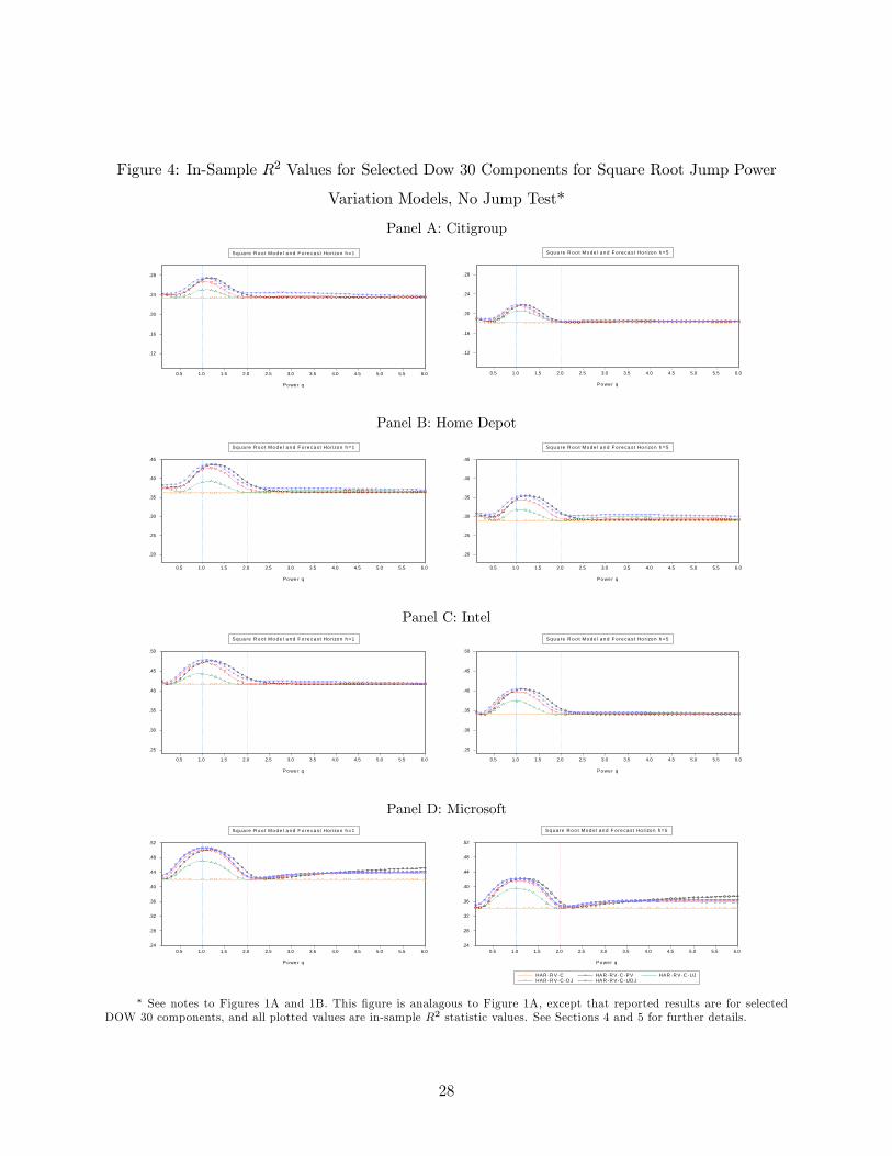
Figure 4: In-Sample 2 Values for Selected Dow 30 Components for Square Root Jump Power

Variation Models, No Jump Test*

Panel A: Citigroup

.12

.16

.20

.24

.28

0.5 1.0 1.5 2.0 2.5 3.0 3.5 4.0 4.5 5.0 5.5 6.0

Po we r q

S q u a re R o o t M o d e l a n d F o re ca s t Ho r izo n h =1

.12

.16

.20

.24

.28

0.5 1.0 1.5 2.0 2.5 3.0 3.5 4.0 4.5 5.0 5.5 6.0

Po we r q


Panel B: Home Depot

.20

.25

.30

.35

.40

.45

0.5 1.0 1.5 2.0 2.5 3.0 3.5 4.0 4.5 5.0 5.5 6.0

Po we r q


.20

.25

.30

.35

.40

.45

0.5 1.0 1.5 2.0 2.5 3.0 3.5 4.0 4.5 5.0 5.5 6.0

Po we r q


Panel C: Intel

.25

.30

.35

.40

.45

.50

0.5 1.0 1.5 2.0 2.5 3.0 3.5 4.0 4.5 5.0 5.5 6.0

Po we r q


.25

.30

.35

.40

.45

.50

0.5 1.0 1.5 2.0 2.5 3.0 3.5 4.0 4.5 5.0 5.5 6.0

Po we r q


Panel D: Microsoft

.24

.28

.32

.36

.40

.44

.48

.52

0.5 1.0 1.5 2.0 2.5 3.0 3.5 4.0 4.5 5.0 5.5 6.0

Po we r q


.24

.28

.32

.36

.40

.44

.48

.52

0.5 1.0 1.5 2.0 2.5 3.0 3.5 4.0 4.5 5.0 5.5 6.0

P o we r q

HAR -R V-C HA R -R V -C -P V HAR -R V -C -UJHAR -R V-C -D J HA R -R V -C -UD J


∗ See notes to Figures 1A and 1B. This figure is analagous to Figure 1A, except that reported results are for selected

DOW 30 components, and all plotted values are in-sample 2 statistic values. See Sections 4 and 5 for further details.

28

Figure 5: Out-of-Sample 2 Values for Selected Dow 30 Components for Square Root

HAR-RV-C-LJ () Model, No Jump Test*

Panel A: Citigroup

.40

.45

.50

.55

.60

.65

5 10 15 20 25 30 35 40 45 50

HAR-RV-C-LJ


.40

.45

.50

.55

.60

.65

5 10 15 20 25 30 35 40 45 50

HAR-RV-C-LJ


Panel B: Home Depot

.20

.22

.24

.26

.28

.30

5 10 15 20 25 30 35 40 45 50

HAR-RV-C-LJ


.20

.22

.24

.26

.28

.30

5 10 15 20 25 30 35 40 45 50

HAR-RV-C-LJ


Panel C: Intel

.20

.25

.30

.35

.40

.45

5 10 15 20 25 30 35 40 45 50

HAR-RV-C-LJ


.20

.25

.30

.35

.40

.45

5 10 15 20 25 30 35 40 45 50

HAR-RV-C-LJ

Square Root Model and Forecat Horizon h=5

Panel D: Microsoft

.15

.18

.20

.23

.25

.28

.30

.33

.35

5 10 15 20 25 30 35 40 45 50

HAR-RV-C-LJ


.15

.18

.20

.23

.25

.28

.30

.33

.35

5 10 15 20 25 30 35 40 45 50

HAR-RV-C-LJ


∗ This figure is analagous to Figure 3, except that reported results are for selected DOW 30 components. See Sections 4

and 5 for further details.

29

empirical evidence on the importance of aggregation

Documents