An ESRC Research Group

Empirical determinants of corruption: A sensitivity analysis

GPRG-WPS-012

Danila Serra

Global Poverty Research Group

Website: http://www.gprg.org/

The support of the Economic and Social Research Council (ESRC) is gratefully acknowledged. The work was part of the

programme of the ESRC Global Poverty Research Group.

Empirical determinants of corruption:

A sensitivity analysis∗

Danila Serra†

Revised: June 2004

Abstract

Many variables have been proposed by past studies as significant determinants of corrup-

tion. This paper asks if their estimated impact on corruption is robust to alteration of the

information set. A "Global Sensitivity Analysis", based on the Leamer’s Extreme-Bounds

Analysis gives a clear answer: five variables are robustly related to corruption. Corruption

is lower in richer countries, where democratic institutions have been preserved for a long

continuous period, and the population is mainly Protestant. Corruption is instead higher

where political instability is a major problem. Finally, a country’s colonial heritage appears

to be a significant determinant of present corruption.

JEL Classification: D72, D73, H11

Key words: corruption, determinants, sensitivity, robustness, extreme-bounds.

∗I am grateful to Oriana Bandiera, Eliana La Ferrara, Guido Tabellini and an anonymous referee for their usefulcomments and suggestions. I am also indebted to Francesco Daveri and Andrea Galeotti for precious discussionson the main idea of the paper.

†CSAE, Department of Economics, University of Oxford. danila.serra@economics.ox.ac.uk

1

Danila Serra

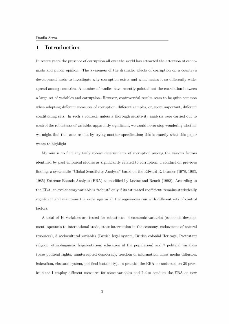
1 Introduction

In recent years the presence of corruption all over the world has attracted the attention of econo-

mists and public opinion. The awareness of the dramatic effects of corruption on a country’s

development leads to investigate why corruption exists and what makes it so differently wide-

spread among countries. A number of studies have recently pointed out the correlation between

a large set of variables and corruption. However, controversial results seem to be quite common

when adopting different measures of corruption, different samples, or, more important, different

conditioning sets. In such a context, unless a thorough sensitivity analysis were carried out to

control the robustness of variables apparently significant, we would never stop wondering whether

we might find the same results by trying another specification; this is exactly what this paper

wants to highlight.

My aim is to find any truly robust determinants of corruption among the various factors

identified by past empirical studies as significantly related to corruption. I conduct on previous

findings a systematic “Global Sensitivity Analysis” based on the Edward E. Leamer (1978, 1983,

1985) Extreme-Bounds Analysis (EBA) as modified by Levine and Renelt (1992). According to

the EBA, an explanatory variable is “robust” only if its estimated coefficient remains statistically

significant and maintains the same sign in all the regressions run with different sets of control

factors.

A total of 16 variables are tested for robustness: 4 economic variables (economic develop-

ment, openness to international trade, state intervention in the economy, endowment of natural

resources), 5 sociocultural variables (British legal system, British colonial Heritage, Protestant

religion, ethnolinguistic fragmentation, education of the population) and 7 political variables

(base political rights, uninterrupted democracy, freedom of information, mass media diffusion,

federalism, electoral system, political instability). In practice the EBA is conducted on 28 prox-

ies since I employ different measures for some variables and I also conduct the EBA on new

2

Danila Serra

variables generated by employing the principal component analysis on highly correlated explana-

tory variables. Unfortunately many explanatory variables which have been included by past

studies among the potential determinants of corruption are clearly endogenous. One should be

aware that for these factors the EBA could only identify robust correlations, whereas the causal

direction remains an open issue which is possibly left to future research.

This paper also makes a contribution to the EBA methodology: for the first time, to the

best of my knowledge, the robustness check is conducted on vectors of dummies instead of a

single variable of interest. I indeed test the robustness of 2 vectors of dummies: a legal vector,

composed by all the legal origin dummies introduced by La Porta et al. (1998), and a colonial

vector accounting for each country’s colonial heritage.

The data employed cover a total of 62 countries, both developed and developing; the measure

of corruption used is the Graft index by Kaufmann et al.(1998). I also check my findings by

replacing Graft with the average value of Corruption Perception Index (CPI by Transparency

International) for the period 1997-1999.

The EBA results strongly support the work by Treisman (2000) and can be summarized as

follows. Five variables passed the Extreme Bounds Analysis. These are: economic development,

Protestant religion, colonial heritage, uninterrupted democracy and political instability. First,

the estimates show a negative strong correlation between economic development and corruption:

as theoretically predicted and empirically shown by previous studies, corruption is lower in richer

countries. Second, the dummy for uninterrupted democracy shows a strong statistically significant

coefficient with the predicted negative sign in all the regression run. As Treisman (2000) pointed

out, what seems to reduce corruption is not the actual level of democracy, but whether a country

has maintained democratic institutions for a long continuous time. Third, the regressions run for

political instability suggests that a higher level of political instability is associated with a higher

level of overall corruption. Fourth, countries where citizens are prevalently Protestant seem to

be less corruption, as previously documented by La Porta et al. (1999) and Treisman (2000).

3

Danila Serra

Finally the robustness of the colonial vector provides evidence that a country’s colonial history

did play a role in determining its actual level of corruption. This result strongly supports the

arguments and findings of Tresiman (2000) that it might be a country’s "legal culture" rather

than the presence of a common low legal system that directly influences corruption.

This paper makes a contribution to the empirical literature that seeks to understand the

causes of corruption. In particular the sensitivity analysis implemented shows that most variables

presented as robust in previous studies are instead highly sensitive to changes in the empirical

specification. A number of measures are taken in order to prevent the EBA results to be driven

by multicollinearity among the explanatory variables. When this is the case the correlations

that could bias the EBA findings are highlighted. Moreover, the unlikelihood to pass this highly

demanding test should be seen as an additional reason to believe that those variables which

succeded are undoubtely related with corruption.

The paper is organized as follows. Section 2 briefly presents the primary findings and contro-

versies of the empirical literature on corruption’s determinants. Section 3 and Section 4 describe

the specific estimate process and the data used. Section 5 discusses the empirical results and

Section 6 summarizes the main findings.

2 Controversies in the Empirical Literature

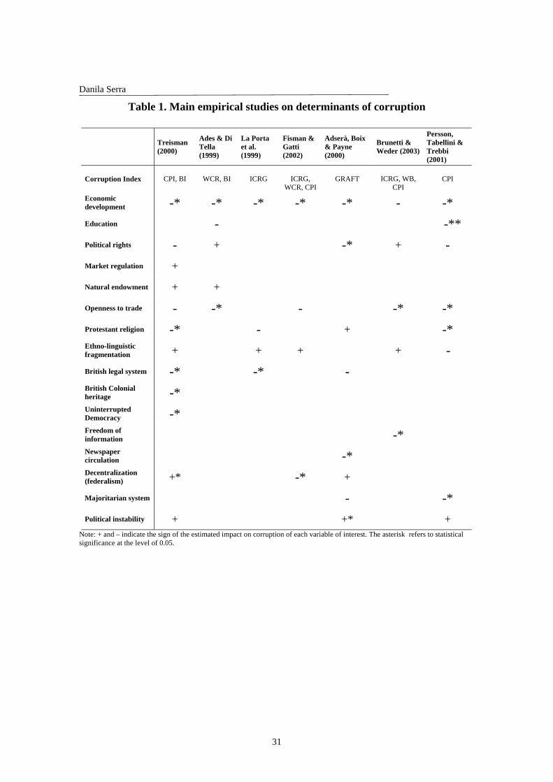
When looking at the most recent and relevant empirical contributions on corruption’s determi-

nants, summarized in Table 1, one should first note the wide consensus in the literature about the

existence of some negative correlation between corruption and economic development. Any em-

pirical study on this matter includes, indeed, some proxy for economic development (mostly

per capita GDP) among the explanatory variables. In contrast, the other explanatory variables

usually vary among studies by different authors. Moreover, it is possible to find factors which

change sign and/or statistical significance from one study to another, based on slightly different

4

Danila Serra

empirical specifications.

-Table 1 -

La Porta, Lopez-de-Silanes, Shleifer and Vishny (1997, 1999) document for instance the rel-

evance of a country’s legal system and religious affiliation in causing corruption; however,

the same variables lose statistical significance in the work by Adserà, Boix and Payne (2000) who

instead point out how corruption may be significantly lowered by the diffusion of daily news-

papers in a democratic context. Also Brunetti and Weder (2003) focus on the negative impact

that citizens’ information may have on corruption, but only when freedom of information is

guaranteed1.

Ades and Di Tella (1999) suggest that openness to foreign trade is a primary factor for

experiencing relatively low corruption. Leite and Weidmann (1999) achieve similar results for

openness by using a different proxy and also point out the positive impact that a country’s en-

dowment of natural resources can have on corruption. Treisman (2000), however, documents

the fragility of the same variable when controlling for development and uninterrupted democracy.

The role of government decentralization in causing corruption is also object of a ferment

debate. On the one hand Fisman and Gatti (2002), among the others, provide evidence of a

negative impact on corruption (i.e. fiscal decentralization leads to less corruption); on the other

hand Treisman (2000) claims a negative correlation between corruption and a federal dummy.

Persson, Tabellini and Trebbi (2001) focus instead on electoral rules; they show how corruption

is lower where electoral systems are pure majoritarian, based on single-member district, plurality

rule and no voting list. Nevertheless Adserà, Boix and Payne (2000) find the dummy for an

electoral system based on proportional representation statistically insignificant. The study by

Treisman (2000) seems to be the most exhaustive, for the objective of this work, for he tries to

find out what causes corruption by controlling for the most wide set of explanatory factors. The

main result of his analysis is the significant impact on corruption of economic development,

Protestant religion, British colonial heritage and democracy uninterrupted for a 46 years

5

Danila Serra

period (1950-1995).

The measurement of corruption increases the difficulty of conducting any empirical study on it.

All the available data are perception indexes provided by private firms and international organi-

zations based on surveys of country citizens or business analysts. These values are far from being

objective measures. Further, these corruption perception indexes could give even more distort

information since the main aim of institutions providing corruption data is to give some country

risk assessments to international investors. According to this view, simple corruption perception

indexes, produced by individual sources, like BI (Business International), ICRG (International

country Risk Guide), WB (World Bank index), WCR (World Competitiveness Report), should

be less reliable than aggregate corruption indicators, like CPI (Corruption perception Index by

Transparency International) and Graft (by Kaufmann, Kraay and Zoido-Lobatòn, 1998) that,

being based on corruption data coming from different sources, include perceptions by citizens as

well as by risk analysts and experts2.

After this brief illustraton of how different corruption indicators, samples of countries, and,

more importantly, empirical specifications might have driven opposite conclusions reached by

previous studies, I look for robust correlations between each explanatory variable and corruption.

3 Extreme Bounds Analysis: Empirical Methodology

Edward E. Leamer (1978), in explaining the common estimation approach used by econometri-

cians, reports this emblematic sentence:

”If you torture data long enough, Nature will confess”

(Coase)

Trying several specifications and choosing the one most favorable to the desired empirical

result, is exactly what this work wants to avoid. I apply to 16 potential determinants of corruption

6

Danila Serra

(the same displayed in the first column of Table 1) a “global sensitivity analysis” based on the

Leamer’s (1978, 1983, 1985) Extreme Bounds Analysis (EBA) as modified by Levine and Renelt

(1992) in their study of growth regressions.

The EBA relies on linear OLS regressions of the following form:

C = α+ βM + γiI+ δzZ

where the dependent variable is the level of corruption perceived in each country according

to the GRAFT index, composed by Kaufmann, Kraay and Zoido-Lobaton (1998), M is the

variable of interest that I want to test, I is a set of basic control variables always included in the

regression, while Z is a set of up to three variables chosen from the most relevant explanatory

factors considered by past studies (see table 1). I choose to have per capita income as the only

I-variable in the EBA specification, for it has been included in any empirical study on corruption

and always found strongly statistically significant3.

The EBA consists of estimating β by modifying the number and the composition of the

conditioning information set Z. If the extreme upper bound and the extreme lower bound of

coefficient β - respectively defined as the estimated coefficients corresponding to the highest

value of β plus twice its standard error and the lowest value of β minus twice its standard error,

result statistically significant (at the conventional level) and with the same sign, the variable M

is considered robust to specification changes4. Note that the Extreme-Bounds Analysis does not

provide support to any causal links between the dependent variable and the M-variable, even if

it results robust; that is, even if a right-hand variable passes the test, it cannot be considered

a robust “determinant” of corruption unless there are no doubts about the causality of the

correlation identified by the EBA.

This paper also presents an extension of the typical Extreme-Bounds Analysis: the test is for

the first time, to the best of my knowledge, applied to vectors of dummies (a legal vector and a

7

Danila Serra

colonial vector). In this case the sensitivity analysis consists in testing the joint significance of

the dummies composing the vector. The estimation steps do not change: the significance of the

M-vector (i.e. an F-value larger than the critical value) is studied when changing the conditioning

set of variables as described above.

The Extreme Bounds Analysis has been criticized for being a too “draconian” in its way of

distinguishing among fragile and robust variables (see Sala-i-Martin, 1997). The most relevant

objection concerns the multicollinearity problems involved when adding Z-variables to the base

specification. A high correlation between the M-variable and just one Z-variable could indeed

induce the loss of significance of β whenever the collinear variable is controlled for. Moreover, an

extremely volatile sign of β could be the result of the presence/absence of the collinear variable/s

in the specification.

In order to deal with this problem, I first modify the original Leamer’s sensitivity analysis

following the suggestions of Levine and Renelt (1992). More in detail, I restrict the number of

explanatory variables in the specification model to a maximum of 5 when three Z-variables are

added. Further, when testing the robustness of one variable, I drop from the control factors

those proxies likely to measure highly related aspects. For example, when I apply the EBA to

the dummy for pure majoritarian electoral rule (maj ) I drop the proxies for the dimension of the

electoral district (dismag) and percentage of vote on list (plist).

The most important measure taken to handle multicollinearity is the registration of the num-

ber of regressions which show an insignificant estimated coefficient of the M- variable. In this

way, sensitivity results for all the variables of interest are easily comparable, making it possible

to understand whether one variable did not pass the EBA due to collinearity with one or more

control factors or to its “truly fragile” nature. If indeed all or almost all the regressions run lead

to an insignificant coefficient we can confidently consider that M-variable as fragile. If the num-

ber of insignificant regressions is instead low compared to the total we could mistake the EBA

results if we declared M as fragile before taking a closer look at the Z-variables entering the

8

Danila Serra

few insignificant regressions. This would make it possible to motivate the failures of the "almost

robust" M-variable and, in this way, distinguish between its truly fragile nature and collinearity

biases.

As an additional attempt to tackle potential collinearity I finally apply principal component

analysis (pca) to two groups of explanatory variables whose correlation with corruption is thought

of as capturing the same economic, sociocultural or institutional aspects. I then conduct the EBA

on the first component which, as I will explain in the next session, accounts in both cases for

more than 65 per cent of the total variance.

3.1 Data Description

The analysis is based on cross-country data covering a total of 62 countries, both developed and

developing. The sample could have been larger since for some variables more than 62 observations

were available, but I choose to restrict the sample in order to have each variable covering the

same countries and, therefore, to lower the chance to bias the estimates. Almost all economic,

sociocultural and institutional variables used in this study refer to average values over the period

1990-1998.

I test the robustness of 16 variables (shown in the first column of Table 1), for a total of

28 proxies (i.e. 28 M variables) since for some variables I check the results by using alternative

measures. For each M-variable the test relies on a total of 299 regressions, with the exception of

the 377 regressions for the I-variable. I also consider a vector of legal origin dummies, found by

La Porta et al. (1998) to be significantly related to corruption, and a vector of colonial heritage

dummies claimed to be highly predictive of corruption by Tresiman (2000).

To measure corruption I employ two aggregate perception indicators: the Corruption Percep-

tion Index (CPI) by Transparency International and the Graft Index by Kaufmann, Kraay and

Zoido-Lobaton (1999). Both measures are based on single perception indexes computed from

9

Danila Serra

surveys of business people, local citizens or experts’ opinions. The aggregation of corruption val-

ues coming from different sources should lower the measurement error intrinsic to any subjective

measure.

The primary differences between the 2 indicators is the aggregating methodology. The Graft

index aggregates individual corruption indicators by using an unobserved components model

which presents the corruption values coming from each source as a linear function of the un-

observed component (the existing true corruption) plus a disturbance term which reflects the

perception errors and the lack of sample coincidence among individual indicators5. The Graft

index is based on data coming from 11 institutional sources and it ranges from a minimum of -2.5

(lack of corruption) to a maximum of 2.5 (worst corruption). The CPI is instead constructed as

a simple mean of values from individual sources opportunely standardized and equally weighted.

I employ the average value of CPI for the period 1997-1999. In 1997 the CPI is constructed by

aggregating corruption data from 6 different sources (for a total of 7 surveys), while in 1998 the

sources included are 7 (for a total of 12 surveys) and 10 (for 14 surveys) in 1999. It assumes values

ranging from 0 (worst corruption) to 10 (lack of corruption). I rescaled both indicators in order

to have higher values associated with higher corruption. It is worth noting that although the CPI

and the Graft index are not based on the same number and types of individual corruption indexes

and rely on different aggregation methodologies, they appear to be highly correlated (ρ = 97). A

strong correlation between indexes is especially important in the context of subjective measures

for it is most likely to reflect consistency in the evaluations and individual perceptions coming

from different sources6.

• I-Variables Data

The only I-variable included the model is economic development proxied by the logarithm of

GDP per capita, adjusted for purchasing power (lyp).

• Economic Data

10

Danila Serra

Among the economic explanatory variables, the presence of State regulation of the economy

is proxied by the “regulatory burden” (reg) constructed by Kaufmann et al. (1999) to take into

account the incidence of market-unfriendly policies on illicit rent appropriation. Higher values

indicate less government intervention. The endowment of natural resources is measured as the

fraction of GDP produced in the Mining and Quarrying sectors (mining).

To test the robustness of a country’s openness to foreign trade I consider 3 alternative proxies:

the sum of exports and imports of goods and services measured as a share of GDP (trade), the

sum of merchandise exports and imports divided by the value of GDP measures in current US

dollars (open), and an index compiled by Sachs and Warner (1995) measuring the fraction of

years during the period 1950-1994 that the economy has been open, ranging from 0 to 1 scale

(yrsopen).

Trade policies and market-unfriendly policies are theoretically related to corruption for similar

reasons. The imposition of tariffs or quantitative restricton as well market regulations are indeed

thought of as creating more opportunities for rent appropriation by providing public officials a

higher discretionary power. A principal component analysis highlighting the common features of

the two variables is therefore sensible, in order to reduce collinearity biases potentially generated

by the inclusion of both reg and open or yrsopen in the specification. The first component, which

I call government intervention (inter) and explains 67 per cent of the variation, is then screened

for robustness according to the EBA approach.

• Sociocultural Data

Protestant religion is measured as the percentage of the population belonging to the Protes-

tant religion in 1980 (prot80). For the ethnolinguistic fragmentation I employ 2 proxies: avelf

and ethno. They capture the probability that two randomly selected persons from a given coun-

try will not belong to the same ethnolinguistic group; they both range from 0 (homogeneous)

to 1 (strongly fractionalized). The level of education is measured as the average educational

11

Danila Serra

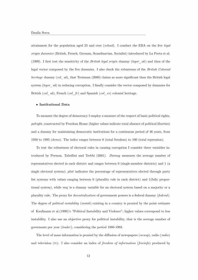
attainment for the population aged 25 and over (school). I conduct the EBA on the five legal

origin dummies (British, French, German, Scandinavian, Socialist) introduced by La Porta et al.

(1999). I first test the sensitivity of the British legal origin dummy (legor_uk) and then of the

legal vector composed by the five dummies. I also check the robustness of the British Colonial

heritage dummy (col_uk), that Treisman (2000) claims as more significant than the British legal

system (legor_uk) in reducing corruption. I finally consider the vector composed by dummies for

British (col_uk), French (col_fr) and Spanish (col_es) colonial heritage.

• Institutional Data

To measure the degree of democracy I employ a measure of the respect of basic political rights,

polright, constructed by Freedom House (higher values indicate total absence of political liberties)

and a dummy for maintaining democratic institutions for a continuous period of 46 years, from

1950 to 1995 (demo). The index ranges between 0 (total freedom) to 100 (total repression).

To test the robustness of electoral rules in causing corruption I consider three variables in-

troduced by Persson, Tabellini and Trebbi (2001). Dismag measures the average number of

representatives elected in each district and ranges between 0 (single-member districts) and 1 (a

single electoral system); plist indicates the percentage of representatives elected through party

list systems with values ranging between 0 (plurality rule in each district) and 1(fully propor-

tional system), while maj is a dummy variable for an electoral system based on a majority or a

plurality rule. The proxy for decentralization of government powers is a federal dummy (federal).

The degree of political instability (instab) existing in a country is proxied by the point estimate

of Kaufmann et al.(1999)’s “Political Instability and Violence”; higher values correspond to less

instability. I also use an objective proxy for political instability, that is the average number of

governants per year (leader), considering the period 1980-1993.

The level of mass information is proxied by the diffusion of newspapers (newsp), radio (radio)

and television (tv). I also consider an index of freedom of information (freeinfo) produced by

12

Danila Serra

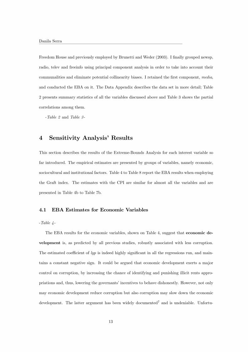
Freedom House and previously employed by Brunetti and Weder (2003). I finally grouped newsp,

radio, telev and freeinfo using principal component analysis in order to take into account their

communalities and eliminate potential collinearity biases. I retained the first component, media,

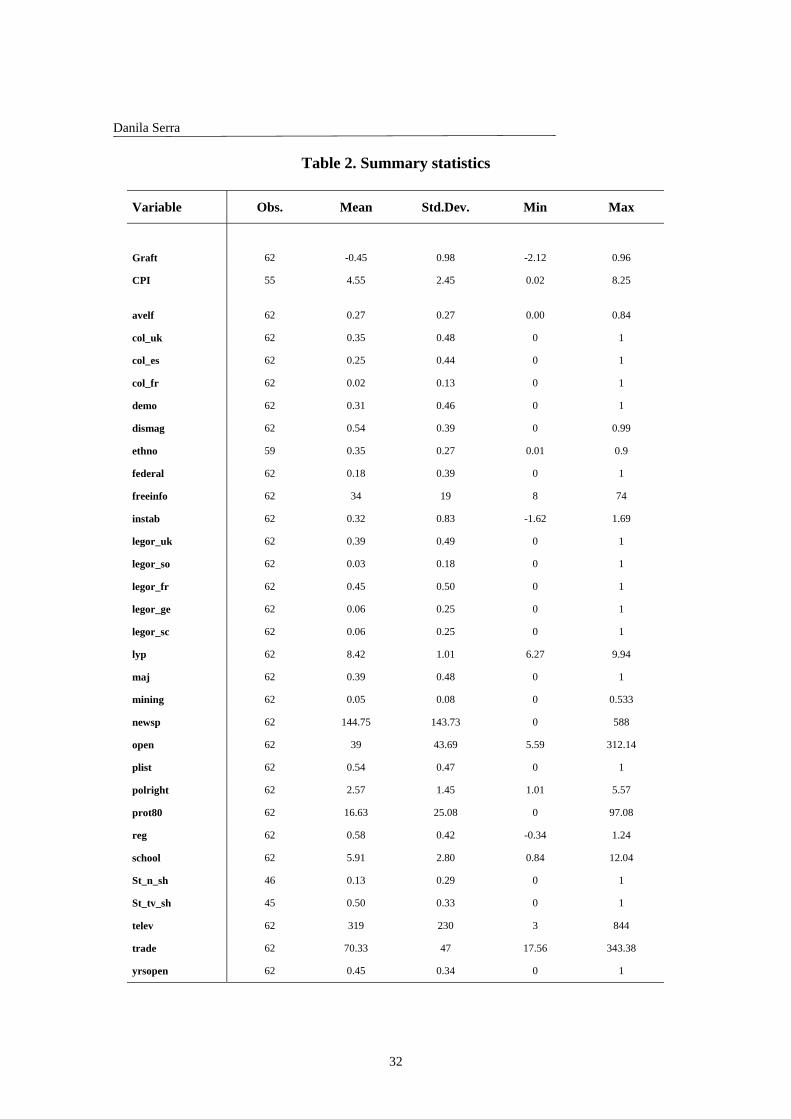
and conducted the EBA on it. The Data Appendix describes the data set in more detail; Table

2 presents summary statistics of all the variables discussed above and Table 3 shows the partial

correlations among them.

-Table 2 and Table 3 -

4 Sensitivity Analysis’ Results

This section describes the results of the Extreme-Bounds Analysis for each interest variable so

far introduced. The empirical estimates are presented by groups of variables, namely economic,

sociocultural and institutional factors. Table 4 to Table 8 report the EBA results when employing

the Graft index. The estimates with the CPI are similar for almost all the variables and are

presented in Table 4b to Table 7b.

4.1 EBA Estimates for Economic Variables

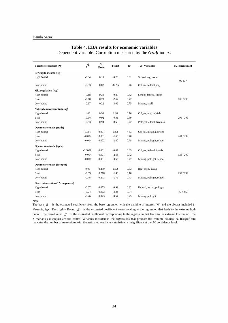
-Table 4 -

The EBA results for the economic variables, shown on Table 4, suggest that economic de-

velopment is, as predicted by all previous studies, robustly associated with less corruption.

The estimated coefficient of lyp is indeed highly significant in all the regressions run, and main-

tains a constant negative sign. It could be argued that economic development exerts a major

control on corruption, by increasing the chance of identifying and punishing illicit rents appro-

priations and, thus, lowering the governants’ incentives to behave dishonestly. However, not only

may economic development reduce corruption but also corruption may slow down the economic

development. The latter argument has been widely documented7 and is undeniable. Unfortu-

13

Danila Serra

nately the Extreme-Bounds Analysis can only establish robust linear correlations and therefore

cannot solve the causation problem. Future research on causes of corruption should therefore

carefully address the endogeneity problem existing in the robust correlation between corruption

and economic development8.

Previous studies argue that the higher the governmental role in the economic sphere, the more

will be the occasions for illicit appropriations of resources by public officials. The EBA shows,

however, the fragility of the market regulation proxy (reg). As shown on Table 4, even though

reg presents the theoretically expected negative sign (i.e. more corruption associated with more

market regulations) its estimated coefficient loses statistical significance in more than 30 per cent

of the regressions run. Equally, none of the 3 proxies for openness to foreign competition is

robust, and among them only open maintains a constant negative sign, as theoretically expected,

but it still loses statistical significance in nearly 40 per cent of the regressions run.

Better results are obtained for the first component retained from the principal component on

the trade variables and the regulations index. Inter presents indeed a contsant negative sign and

looses significance in 47 out of 232 regressions run. The main cause of this lack of significance

in relatively few regressions seems to be the inclusion of the proxy for political instability in the

specification. Inter and instab are indeed highly correlated (ρ = 0.72); government intervention

in the economy appears to be higher the lower political instability is9, yet political instability, as

we will see later, is robustly negatively related to corruption. Finally, the proxy for endowment

of natural resources also comes out as fragile. Our result replicates those of Treisman (2000);

the estimated impact of natural endowment on corruption disappears when adopting specification

comprehensive of proxies for economic development and uninterrupted democracy.

4.2 EBA Estimates for Sociocultural Variables

Recent empirical studies (see La Porta et al., 1997, 1999, and Treisman, 2000) point out the

positive or negative impact that different religions may have on corruption. This could be due,

14

Danila Serra

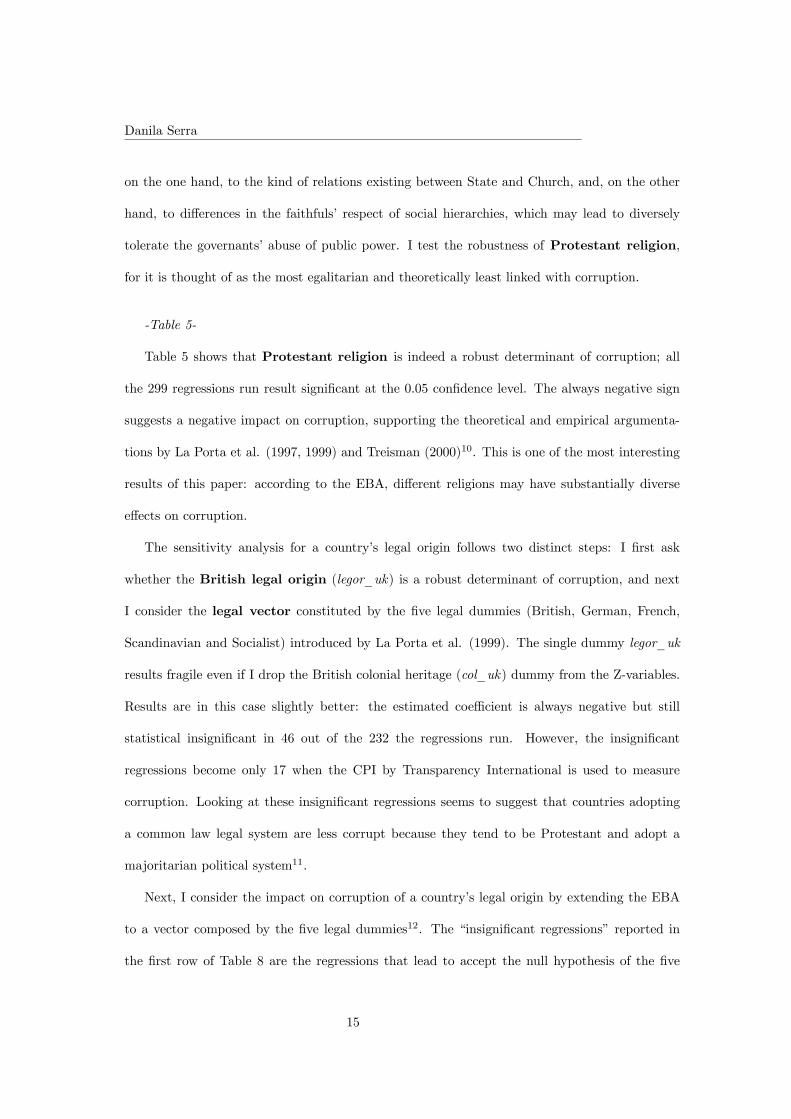
on the one hand, to the kind of relations existing between State and Church, and, on the other

hand, to differences in the faithfuls’ respect of social hierarchies, which may lead to diversely

tolerate the governants’ abuse of public power. I test the robustness of Protestant religion,

for it is thought of as the most egalitarian and theoretically least linked with corruption.

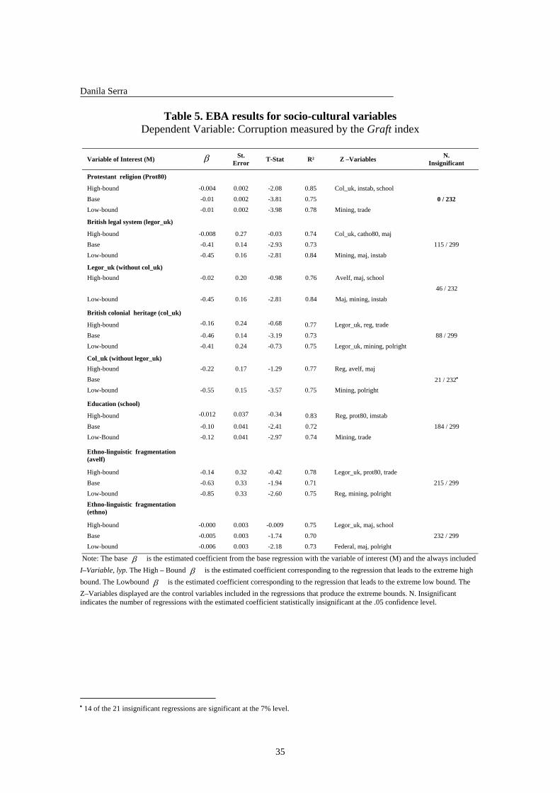
-Table 5-

Table 5 shows that Protestant religion is indeed a robust determinant of corruption; all

the 299 regressions run result significant at the 0.05 confidence level. The always negative sign

suggests a negative impact on corruption, supporting the theoretical and empirical argumenta-

tions by La Porta et al. (1997, 1999) and Treisman (2000)10. This is one of the most interesting

results of this paper: according to the EBA, different religions may have substantially diverse

effects on corruption.

The sensitivity analysis for a country’s legal origin follows two distinct steps: I first ask

whether the British legal origin (legor_uk) is a robust determinant of corruption, and next

I consider the legal vector constituted by the five legal dummies (British, German, French,

Scandinavian and Socialist) introduced by La Porta et al. (1999). The single dummy legor_uk

results fragile even if I drop the British colonial heritage (col_uk) dummy from the Z-variables.

Results are in this case slightly better: the estimated coefficient is always negative but still

statistical insignificant in 46 out of the 232 the regressions run. However, the insignificant

regressions become only 17 when the CPI by Transparency International is used to measure

corruption. Looking at these insignificant regressions seems to suggest that countries adopting

a common law legal system are less corrupt because they tend to be Protestant and adopt a

majoritarian political system11.

Next, I consider the impact on corruption of a country’s legal origin by extending the EBA

to a vector composed by the five legal dummies12. The “insignificant regressions” reported in

the first row of Table 8 are the regressions that lead to accept the null hypothesis of the five

15

Danila Serra

dummies’ coefficients jointly equal to zero.

-Table 8-

Results seem to confirm the findings obtained for legor_uk. The loss of statistical joint

significance of the legal vector 31 regressions (only 18 when the Transparency Index is employed

for corruption) is indeed due to the inclusion of the British colonial dummy, the Protestant

religion and the majoritarian political system in the empirical specification.

Treisman (2000) claimed that what really matters on corruption is not a country’s legal

system but its “legal culture”, strongly linked with its colonial heritage. The Extreme-Bounds

Analysis applied to the British Colonial heritage provides indeed better results compared to

the British legal origin’s ones. What comes out is that not only does col_uk lose significance

in a lower number of regressions than legor_uk but if legor_uk is dropped from the set of

Z-variables, col_uk results nearly robust. Only 21 regressions present indeed an insignificant

estimated coefficient; moreover, 14 out of 21 are significant at the 0.07 confidence level. Results

obtained with the CPI are even better, with col_uk always significant when legor_uk is excluded

from the set of Z-variables.

The different EBA results found for the British colonial heritage and the British legal origin

suggest that the reason for observing relatively lower levels of corruption in former British colonies

goes somehow behind the adoption of a common law legal system, as Treiman (2000) has pointed

out. This result is confirmed when the EBA is conducted on the vector composed by the colonial

dummies; the colonial vector is indeed significant in all the 299 regressions run, with the British

colonial dummy being the only one showing a negative sign. Colonial traditions seem therefore

to play a consistently significant role in determing the present level of perceived corruption.

To conclude, Table 5 reports the EBA results for education of the population and ethno-

linguistic fragmentation. As it is clear from the number of insignificant regressions and from

the sign of the coefficients’ bounds, both variables are highly sensitive to changes in the control

16

Danila Serra

factors included in the empirical specification13.

4.3 EBA Estimates for Institutional Variables

It is a common belief that incentives and opportunities of generating corruption are strongly

linked with political institutions; therefore, the empirical literature on determinants of corruption

includes many institutional factors among the potential causes of corruption.

The presence of democratic institutions is one of the main factors considered by past

studies on corruption’s determinants. On a theoretic viewpoint, illicit governants’ behavior can

be prevented only when basic political rights are effectively guaranteed to citizens. Unfortunately,

it is also true that corrupt governants are more likely to limit the citizens’ control on their power

through the instrument of vote. Therefore, due to simultaneity problems, even if some proxy

for democracy resulted robust, we should not stop wondering about the causal direction of that

correlation. According to the EBA, actual democracy (polright) is weakly related with corruption

whereas uninterrupted democracy (demo) results highly significant in reducing corruption.

-Table 6-

All the regressions run for demo show indeed a stable negative coefficient, always strongly

statistical significant. Therefore what seems to matter for corruption is not the presence of demo-

cratic institutions newly legitimated and implemented (polright is indeed fragile), but democratic

principles consolidated during a long continuous period (see also Treisman, 2000). In other words,

it seems that civic participation to political activities is effective in increasing the risk for corrupt

incumbents being caught and punished (i.e. less incentives to illicit rent appropriation) only if

democratic institutions are so rooted in a country to make political elections really a mean of

control over governants’ activities. Note that the use of such a proxy for continuous democratic

institutions also removes the simultaneity problem.

It is also a common opinion that every democratic regime should grant some basic rights such

17

Danila Serra

as freedom of expression and information. Theoretically, if the electorate is not sufficiently

and correctly informed, the vote will not be an efficient instrument to control public corruption.

However, the three proxies for the degree of mass media diffusion among citizens, radio, tv, and

newsp, result fragile. Nevertheless, as pointed out by Besley, Burgess and Prat (2002), a proxy

for the diffusion of mass media could be a biased measure of citizens’ degree of information for

it does not consider the lack of freedom normally experienced by journalists. Political pressures

on media could in fact inhibit the diffusion of news on corrupt acts, vanishing, in this way the

theoretic negative impact of media on corruption. This is why I also check the sensitivity of

the freedom of information index14. As shown on Table 6, although freeinfo conserves the

predicted sign (positive, since freeinfo assumes higher values when freedom is lower), it loses

statistical significance in nearly all the regressions run. Unsatisfactory results are also obtained

for the first component of the principal component analysis conducted on all the media variables,

freedom of information included. The variable media looses indeed statistical significance in

almost 40 per cent of the regressions run and presents a volatile sign.

The federal dummy also comes out as fragile. Although its constantly positive sign seems

to suggest a positive impact on corruption, its luck of significance in more than 60 per cent of

the regressions does not allow us to claim neither a positive nor a negative correlation between

this variable and corruption.

In order to estimate the impact of electoral rules on corruption I follow the estimation

procedure of the only empirical study (Persson, Tabellini and Trebbi, 2000), to the best of my

knowledge, which deeply investigate the effects of different electoral systems on corruption. I first

consider two related but distinct dimensions of electoral rules, the electoral district magnitude

(dismag) and the percentage of representatives elected on a party list (plist), and then I check

the robustness of the dummy for the majoritarian electoral system (maj ). As shown on Table 6,

none of the proxies maintains a constant sign and/or conserves an acceptable level of statistical

significance. One could argue that the electoral rules can affect corruption only if citizens can

18

Danila Serra

effectively use the instrument of vote, therefore, if I don’t control for this, the electoral proxies

are not expected to be statistical significant. This is the reason why I also apply the EBA to

interactions between a dummy for democracy and all the institutional variables, as I will explain

later.

Finally, table 6 reports the high, robust correlation between political instability and cor-

ruption. The estimated sign is stable and always negative, as theoretically expected: since higher

values of instab mean less political instability, a negative sign suggests indeed that more political

instability (low instab) leads to more corruption (high Graft). This result conforms therefore

to previous studies, claiming that public officials will decide to behave more opportunistically if

there is a high probability of losing their office next period due to political instability. In other

words, incumbents will be more corrupt where high instability lowers the probability of future

rents appropriation15. However, it is also reasonable for corrupt governments to be the cause of

high political instability. Unfortunately once again the EBA cannot solve the reverse causality

problem, which remains a primary open issue which is possibly left to future research.

• The last check: Interactive Terms

To further check the relevance of institutional factors in determining corruption I also take

as M-variable the interaction between each institutional factor and a dummy for currently being

a democracy (demo_c) constructed on the basis of polright, with the value 3 taken as the

benchmark. Many political institutions can indeed have some effects on corruption only if political

rights are sufficiently guaranteed to citizens. The EBA results for the interactive terms16 show the

robustness of “freeinfo*democracy”, which conserves the predicted positive sign and statistical

significance in 213 out of 232 regressions17.

-Table 7-

This outcome suggests that freedom of information does matter in reducing corruption under

condition of political freedom. Also the results for the interaction between electoral district

19

Danila Serra

magnitude (dismag) and democracy seem to be relevant, especially if compared to the EBA

estimates for dismag taken as a single M-variable: the interactive term shows indeed a constant

negative sign and looses statistical in relatively fewer regressions. This means that the magnitude

of the electoral district could have some effect on reducing corruption only if citizens are given

a real control power on governants by means of the electoral consensus. Unfortunately these

results do not hold when the Graft index is replaced by the CPI to measure corruption.

5 Conclusions

This paper’s aim was to test the robustness of previous empirical evidence on corruption’s deter-

minants. I addressed this issue by implementing a global sensitivity analysis based on the E. E.

Leamer’s EBA. Five of the 28 proxies examined reveal to be highly related to perceived corrup-

tion. First, richer countries tend to have less corruption then poorest ones. Second, democratic

institutions do exert a certain control on corruption only when they have been continuously held

for decades. Third, countries characterized by more political instability result to be more cor-

rupt. Fourth, prevalently Protestant countries seem to be less corrupt. Finally colonial heritage

appears to be strongly correlated with the current level of corruption, possibly due to the legal

cultures inherited from the former colonising countries as suggested by Triesman (2000).

The strong requirements of the EBA procedure provide evidence to believe that these five

variables are truly correlated with corruption. The endogeneous nature of economic development,

democratic institutions and political instability remains however an open issue left to future

research on corruption for the EBA cannot solve the causation problem. Due to collinearity

problems, the Extreme-Bounds Analysis does not allow to claim the irrelevance of all the other

explanatory variables which resulted fragile. However, we can still be confident on the true

fragility of those variables, like endowment of natural resources, ethnolinguistic fragmentation

and political rights, which resulted insignificant in all or nearly all the regressions run.

20

Danila Serra

Notes1Further efforts in showing the links between corruption and mass media have recently been

made by Djankov et al. (2003) and Besley et al. (2002), not shown in Table 1, who underline

how media ownership could be crucial in assuring (or preventing) freedom of information.

2Knack and Azfar (2000) underline how the choice of countries to assign a value for corruption

is mainly driven by the interests of foreign investors. This leads, for most corruption indicators, to

small samples of countries, generally representing large markets characterized by low corruption.

The CPI and the Graft index, by aggregating individual corruption indicators, result less biased

toward larger and less corrupt countries.

3In a preliminary analysis I also included a measure of human capital and guarantee of basic

political rights among the I-variables. Their lack of significance in nearly all the regressions run

motivated their subsequent exclusion from the I- matrix.

4See Leamer (1978, 1983) and Levine and Renelt (1992) for details.

5For more details on the estimation procedure, see Kaufmann, Kraay and Zoido-Lobadon

(1999)

6The CPI presents however missing data for the following 7 countries: Bangladesh, Dominican

Repulic, Gambia, Ghana, Papua New Guinea, Sri Lanka, Trinidad and Tobago. The EBA results

employing the CPI could therefore be more biased toward less corrupt countries, compared to

those based on the Graft index.

7See Mauro (1995) among the others.

8Note that Treisman (2000) has already provided evidence for a direct effect of economic

development on corruption (whetever the effect of corruption on economic development is) by

running 2SLS using the distance from the Equator as instrument for per capita income.

9Remember that higher values of instab indicate lower political instability.

10The EBA applied to a proxy for Catholic religion (catho80 ), which is theoretically the most

hierarchical religion and theoretically most linked with corruption, gives similar results with the

21

Danila Serra

opposite sign. High collinearity with prot80 motivates its exclusion from the present analysis.

11Note that the inclusion of maj in the regression makes both the coefficients of legor_uk and

maj insignificant.

12La Porta et al. (1999) distinguish between two main legal system typologies, ”common law”

and ”civil law”, based on the assumption that they essentially differ in the relative power of the

State and private property owners, and, as a consequence, in the levels of protection granted to

individual citizens against abuses of power by public officials. More in detail, distinction is made

among British, French, German, Scandinavian and Socialist legal systems.

13The loss of statistical significance of ethno-linguistic fragmentation when controlling for per

capita income (one of our I-variables) could be explained by argumenting that ethnic fragmenta-

tion has only an indirect effect on corruption by means of economic development (see Treisman,

2000).

14Following Besley et al. (2002) and Djankov et al. (2003), I also applied the EBA to proxies for

state-owned newspapers and tv stations, thought they tend to register “political capture” of the

media rather than potential causes of corruption. More in detail, I considered the market share

of state-owned newspapers/TV stations out of the five largest daily newspapers/TV stations.

However, for these variables the sample used is restricted to only 45 countries.The proxy for

state owned tv stations passed the EBA with a significant negative sign. This result confirms

what has been pointed out by Besley et al.(2002): state owned media are more likely to hide bad

news on the government, such as illicit appropriation of public resources. This would lead to a

lower perception of corruption (but not to less corruption!).

15Using an objective proxy for political instability - the average number of governants per year

(leader) during the period 1980-1993, political instability looses statistical significance in almost

all the regressions run though it conserves the expected positive sign.

16Table 7 reports the EBA results only for those interactions whose estimates present substan-

tial changes compared to the corresponding not interacted estimates.

22

Danila Serra

17The 20 insignificant regressions indicate the presence of collinearity problems due to the

inclusion of instab among the explanatory variables. However the fact that more than 50 regres-

sions with instab entering the specifcation presents a significant coefficient for demo_c*freeinfo

suggests that the resulting negative impact of freedom of information on corruption cannot be

thought of as merely driven by its negative correlation with political instability.

References

[1] Ades, A. and R. Di Tella (1997). National Champions and Corruption: Some Unpleasant

Interventionist Arithmetic. The Economic Journal 107(443): 1023-42.

[2] Ades, A. and R. DI Tella (1999). Rents, Competition and Corruption. American Economic

Review 89: 982-993.

[3] Adserà A. , C. Boix and M. Payne (2000). Are You Being Served? Political Accountability

and Quality of Government. IADP working paper 438.

[4] Besley, T. and R. Burgess (2002). The Political Economy of Government Responsive-

ness:Theory and Evidence from India. The Quarterly Journal of Economics 117: 1415-1452.

[5] Besley, T., R. Burgess and A. Prat (2002). Mass Media and Political Accountability. De-

partment of Economics working paper, London School of Economics, February.

[6] Brunetti A. and B. Weder (2003).A Free Press is Bad News for Corruption, forthcoming,

Journal of Public Economics.check!

[7] Djankov S., C. McLiesh, T. Nenova and A. Shleifer (2003).Who Owns the Media?. Journal

of Law and Economics, forthcoming.

[8] Fisman, R. and R. Gatti (2002). Decentralization and Corruption: Cross-Country and Cross-

State Evidence. Journal of Public Economics 83 (3): 325-345.

23

Danila Serra

[9] Freedom House (2001). Press Freedom Survey 2001.

[10] Kaufmann D., A. Kraay and P. Loido-Zobatòn (1999). Aggregating Governance Indicators.

World Bank working paper 2195.

[11] Kaufmann D., A. Kraay and P. Loido-Zobatòn (1999). Governance Matters. World Bank

working paper 2196.

[12] Kaufmann, D. (1997). Corruption: The Facts. Foreign Policy 107.

[13] Knack S. and O. Azfar (2000). Are Larger Countries Really More Corrupt?. World Bank

working paper 2470.

[14] Lambsdorff, J. G. (1998).Corruption in Comparative Perception. In A. K. Jain (Ed.) The

Economics of Corruption. Kluwer Academic Publishers.

[15] Lambsdorff, J. G. (2000). Background Paper to the 2000 Corruption Perceptions Index.

Framework Document, Transparency International and Göttingen University.

[16] La Porta R., F. Lopez-de-Silanes, A. Shleifer and R.W. Vishny (1997). Trust in Large

Organisations. The American Economic Review, Papers and Proceedings, 87(2): 333-338.

[17] La Porta R., F. Lopez-de-Silanes, A. Shleifer and R.W. Vishny (1999). The Quality of

Government. The Journal of Law, Economics and Organization 15: 222-79.

[18] Leamer E. E. (1978). Specification Searches: Ad Hoc Inference from Non-Experimental Data,

New York: Wiley.

[19] Leamer, E. E. (1983). Let’s take the con out of econometrics. American Economic Review

73(3): 31-43.

[20] Leamer, E. And and L. Herman (1983) “Reporting the Fragility of Regression Estimates”,

Review of Economics and Statistics, 65: 306-17.

24

Danila Serra

[21] Leamer, E. E. (1985), “Sensitivity Analysis Would Help”, American Economic Review, 75

(5): 31-43.

[22] Leite, C. and J. Weidmann (1999) Does Mother Nature Corrupt? Natural Resources, Cor-

ruption and Economic Growth. IMF working paper, 99/85.

[23] Levine, R. and D. Renelt (1992). A Sensitivity Analysis of Cross-Country Growth Regres-

sions. American Economic Review 82(4): 942-963.

[24] Levine, R. and S. Zervos (1993). Looking at the Facts: What we Know about Policy and

Growth from Cross-Country Analysis. World Bank working paper 1115.

[25] Mauro P. (1995). Corruption and Growth. Quarterly Journal of Economics 110: 681-712.

[26] Persson, T. and G. Tabellini (2000). Political Economics: Explaining Economic Policy. MIT

Press.

[27] Persson, T., G. Tabellini and F. Trebbi (2003). Electoral Rules and Corruption. Journal of

the European Economic Association 1(4): 958-989.

[28] Sala-i-Martin, Xavier (1997). I Just Run Four Million Regressions. NBER working paper

6252.

[29] Tanzi, V. (1998). Corruption Around the World: Causes, Consequences, Scope, and Cures.

IMF Staff Papers 45(4).

[30] Treisman, D. (2000). The Causes of Corruption: A Cross-National Study. Journal of Public

Economics 76: 399-457.

[31] World Bank (1997-99). World development report. New York, Oxford University Press.

[32] World Bank (2001). World Development Indicators.

25

Danila Serra

DATA APPENDIX

Dependent Variable

GRAFT = proxy for Political and Bureaucratic Corruption built by Kaufmann et al. (1999).

The index aggregate individual corruption indicators from eleven different sources by using an

unobserved components. Original scores range from -2.5 to 2.5 with higher values corresponding

to better outcome. The index is rescaled to have higher values associated to more corruption.

Source: Kaufmann et al. (1999), available at www.worldbank.org/wbi/gac.

CPI = proxy for Political Corruption and Bureaucratic Corruption published by Trans-

parency International since 1995. The index employed is the average of the CPI (Corruption

Perception Index) over the period 1997-1999. Original scores, ranging from 0 (= completly cor-

rupt) to 10 (= clean) have been rescaled to have higher values associated to more corruption.

Source: Transparency International (www.transparency.de) and Internet Center for Corruption

Research (www.gwdg.de/~uwvw).

• Economic Variables

LYP = logarithm of real GDP per capita in constant dollars (international prices, base

year 1985). Data trough 1992 are taken from the Penn World Table 5.6, while data on the

period 1993-1998 are taken from the Easterly’s series available on the World Bank’s web site on

www.worldbank.org.

MINING = fraction of GDP produced in the Mining and Quarrying sector. Data are for

the year 1988 when possible, or the closest available year. The LYP data have been netted out

of ”mining”. Source: Jones C., Hall E. H., QJE (Feb. 1999).

OPEN = proxy for the degree of a country openness to international competition. It is the

sum of merchandise exports and imports measured in current U.S. dollar divided by the value

of GDP converted to international dollars using purchasing power parity (PPP) rates. Data

26

Danila Serra

are average for years 1997 and 1998. Source: The World Bank’s World Development Indicators

(CD-ROM 2000).

REG = proxy for the extend of State intervention in economic markets. It is the ”Regulatory

Burden”, the fourth cluster of Kaufmann et. al. (1999)’s governance indicators. It focuses on

the government policies including measures of the incidence of market-unfriendly policies such as

price controls or inadequate bank supervision, as well as, on perceptions of the burdens imposed

by excessive regulation in areas such as foreign trade and business development. It ranges from

around -2.5 to around 2.5 with higher values corresponding to better outcome. Source: Kaufmann

et al. (1999a.), available at www.worldbank.org/wbi/gac.

TRADE = proxy for the extend of openness to foreign competition. It is the sum of exports

and imports of goods and services measured as a share of gross domestic product. Source: The

World Bank’s World Development Indicators (CD-ROM 2000).

YRSOPEN = proxy for the extent of openness to foreign competition. The index compiled

by Sachs and Warner (1995), measures the fraction of years during the period 1950-1994 that

the economy has been open and is measured on a [0,1] scale. A country is considered open if

it satisfies all of the following criteria: i) nontariff barriers cover less than 40 percent of trade,

ii) average tariff rates are less than 40 percent, iii) any black market premium was less than 20

percent during the 1970s and 1980s, iv) the Country is not classified as socialist by Kornai [1992]

and v) the government does not monopolize major exports. Source: Jones C., Hall E. H., QJE

(Feb. 1999).

• Sociocultural Variables

AVELF = index of Ethnolinguistic Fractionalization that approximates for the level of lack

of ethnic and linguistic cohesion within a country. It ranges from 0 (homogeneous) to 1 (strongly

fractionalized) and averages 5 different indexes. The components are: 1) Atlas Narodov Mira,

1960; 2) Muller, 1964; Roberts, 1962; 4) and 5) Gunnemark, 1991. Source: La Porta et al.

27

Danila Serra

(1998). For Central and Eastern Europe countries computations follow Mauro (1995) with data

from Quain (1999).

CATHO80 = percentage of the population belonging to the Roman Catholic religion in

1980. The values are in percent (scale from 0 to 100). Source: La Porta et al. (1999).

COL_(ES, FR, UK) = dummy variable taking the value 1 if the country has been a colony

of Spain (or Portugal) (ES), France (FR) or United Kingdom (UK) for a significant time and 0

otherwise. Source: Wacziarg (1996).

ETHNO = index of ethno-linguistic fractionalization that captures the probability that two

randomly selected persons from a given country will not belong to the same ethnolinguistic group.

Source: Mauro (1995) and Taylor C.L., Hudson M.c., World Handbook of Politcal and Social

Indicators II: Cross-National Aggregate Data 1950-1965.

LEGOR_(FR, GE, SC, SO, UK)= dummy variable for the origin of the legal system and,

consequently, of the original electoral law for each Country. Five possible origins are considered:

Anglo-Saxon Common Law (uk), French Civil Law (fr), German Civil Law (ge), Socialist Law

(so), and Scandinavian Law (sc). Source: La Porta et al. (1999).

PROT80= percentage of the population of each Country belonging to the Protestant religion

in 1980. The values are in percent (scale from 0 to 100). Source: La Porta et al. (1999).

SCHOOL = years of schooling (education). Average educational attainment is measured in

1985 for the population aged 25 and over as reported by Barro and Lee (1993). Source: Jones

C., Hall E. H., QJE (Feb. 1999).

• Institutional Variables

DEMO = dummy for continuous democracy from 1950 to 1995. A country is considered

democratic by criteria of Alvarez etal. 1996: (1) the chief executive is elected, (2) the legislature

(at least its lower house) is elected, (3) more that one partycontests elections, and (4) during the

last three elections of a chief executive there has been at least one turnover of power between

28

Danila Serra

parties. Data are from Treisman (2000).

DISMAG = electoral district magnitude. It is a measure of the average number of represen-

tatives elected in each district. It ranges between 0 and 1, taking a value of 0 for a system with

only single-member districts and close to 1 for a system with a single electoral district. Source:

Persson, Tabellini, Trebbi (2000).

FEDERAL = federalism dummy. Source: Boix 2000.

FREEINFO = index of freedom of information provided by Freedom House since 1997

on the basis of the following criteria: 1) laws and regulations that influence media content 2)

political influence over media content; 3) economic influence over media content 4) repressive

actions which constitute violations of press freedom. Values range from 0 (total freedom) to 100

(total repression). Source: Freedom House.

INSTAB = proxy for the possibility to have wrenching changes in government. It is the point

estimate of Kaufmann et al.(1999)’s “Political Instability and Violence”, and ranges from around

-2.5 to around 2.5 (higher values correspond to less political instability). Source: Kaufmann et

al. (1999), available at www.worldbank.org/wbi/gac.

LEADER = number of government leaders in the recent period divided by the length of

period in years. Leader is PM in parliamentary systems, president or head of state in presidential

or non-democracy. Source Rulers database: http//www.geocities.com/Athens/1058/rulers.html.

MAJ= dummy variable taking the value 1 in presence of either a majority or a plurality

rule, 0 otherwise. Only legislative elections are considered. Source: Persson, Tabellini and

Trebbi (2001).

NEWSP = Circulation of daily newspapers, where newspapers are journals published at

least four times a week. Data are for 1996. Source: World Development Indicators, World Bank.

PLIST = percentage of representatives elected through party list systems. It ranges between

0 (under plurality rule in every district) and 1 (in a system with full proportionality). Source:

Persson, Tabellini, Trebbi (2001).

29

Danila Serra

POLRIGHT = proxy for the extend of respect of basic political rights. The index ranges

from 1 (max freedom) to 7 (total absence of political rights). Values are averages of data from

1990/01 to 1998/99 assessments. Source: Freedom house.

RADIO = Number of radio receptors for thousands of inhabitants. Data are for 1999.

Source: World Development Indicators, World Bank.

SNEWSP_SH= The market share of state owned newspapers out of the aggregate market

share of the five largest daily newspapers (by circulation), 1999. Source: Djankov et al. (2001)

STV_SH= The marjet share of state-owned tv stations out of the aggregate market share

of the five largest tv stations (by viewership), 1999. Source: Djankov et al. (2001)

TV = Number of televisions for thousands of inhabitans. Data are for 1999. Source: Inter-

national Telecommunication Union (ITU), World Bank.

30

Danila Serra

31

Table 1. Main empirical studies on determinants of corruption

Treisman (2000)

Ades & Di Tella (1999)

La Porta et al. (1999)

Fisman & Gatti (2002)

Adserà, Boix & Payne (2000)

Brunetti & Weder (2003)

Persson, Tabellini & Trebbi (2001)

Corruption Index CPI, BI WCR, BI ICRG

ICRG, WCR, CPI

GRAFT

ICRG, WB, CPI

CPI

Economic development -* -* -* -* -* - -* Education - -** Political rights - + -* + - Market regulation + Natural endowment + + Openness to trade - -* - -* -* Protestant religion -* - + -* Ethno-linguistic fragmentation + + + + - British legal system -* -* - British Colonial heritage -* Uninterrupted Democracy -* Freedom of information -* Newspaper circulation -* Decentralization (federalism) +* -* +

Majoritarian system - -* Political instability + +* +

Note: + and – indicate the sign of the estimated impact on corruption of each variable of interest. The asterisk refers to statistical significance at the level of 0.05.

Danila Serra

32

Table 2. Summary statistics

Variable Obs. Mean Std.Dev. Min Max

Graft 62 -0.45 0.98 -2.12 0.96

CPI 55 4.55 2.45 0.02 8.25

avelf 62 0.27 0.27 0.00 0.84

col_uk 62 0.35 0.48 0 1

col_es 62 0.25 0.44 0 1

col_fr 62 0.02 0.13 0 1

demo 62 0.31 0.46 0 1

dismag 62 0.54 0.39 0 0.99

ethno 59 0.35 0.27 0.01 0.9

federal 62 0.18 0.39 0 1

freeinfo 62 34 19 8 74

instab 62 0.32 0.83 -1.62 1.69

legor_uk 62 0.39 0.49 0 1

legor_so 62 0.03 0.18 0 1

legor_fr 62 0.45 0.50 0 1

legor_ge 62 0.06 0.25 0 1

legor_sc 62 0.06 0.25 0 1

lyp 62 8.42 1.01 6.27 9.94

maj 62 0.39 0.48 0 1

mining 62 0.05 0.08 0 0.533

newsp 62 144.75 143.73 0 588

open 62 39 43.69 5.59 312.14

plist 62 0.54 0.47 0 1

polright 62 2.57 1.45 1.01 5.57

prot80 62 16.63 25.08 0 97.08

reg 62 0.58 0.42 -0.34 1.24

school 62 5.91 2.80 0.84 12.04

St_n_sh 46 0.13 0.29 0 1

St_tv_sh 45 0.50 0.33 0 1

telev 62 319 230 3 844

trade 62 70.33 47 17.56 343.38

yrsopen 62 0.45 0.34 0 1

Danila Serra

33

Table 3. Simple correlations among variables A

VE

LF

CA

TH

O80

CO

L_E

S

CO

L_F

R

CO

L_U

K

CPI

DE

MO

DIS

MA

G

FED

ER

AL

FRE

EIN

FO

GR

AFT

INST

AB

LE

GO

R_F

R

LE

GO

R_G

E

LE

GO

R_S

C

LE

GO

R_S

O

LE

GO

R_U

K

LY

P

MA

J

MIN

ING

NE

WSP

OPE

N

PLIS

T

POL

RIG

HT

PRO

T80

RA

DIO

RE

G

SCH

OO

L

TE

LE

V

TR

AD

E

YR

SOPE

N

AVELF 1

CATHO80 -0.21 1

COL_ES -0.07 0.65 1

COL_FR 0.25 -0.14 -0.08 1

COL_UK 0.47 -0.43 -0.44 -0.09 1

CPI 0.38 0.40 0.56 0.12 -0.04 1

DEMO -0.33 -0.09 -0.31 -0.09 -0.13 -0.77 1

DISMAG -0.39 0.33 0.30 0.07 -0.51 -0.02 0.06 1

FEDERAL -0.13 0.15 0.11 -0.06 -0.08 -0.14 0.24 -0.09 1

FREEINFO 0.38 -0.18 0.13 0.00 0.30 0.56 -0.59 -0.15 -0.19 1

GRAFT 0.38 0.28 0.46 0.09 0.05 0.97 -0.78 -0.09 -0.20 0.57 1

INSTAB -0.40 -0.07 -0.35 -0.18 -0.17 -0.85 0.66 0.03 0.22 -0.60 -0.83 1

LEGOR_FR -0.22 0.67 0.65 0.14 -0.54 0.53 -0.25 0.45 -0.08 0.03 0.37 -0.29 1

LEGOR_GE -0.17 -0.02 -0.15 -0.03 -0.19 -0.25 0.25 0.13 0.39 -0.27 -0.27 0.34 -0.24 1

LEGOR_SC -0.20 -0.31 -0.15 -0.03 -0.19 -0.47 0.40 0.24 -0.12 -0.17 -0.42 0.35 -0.24 -0.07 1

LEGOR_SO -0.15 0.09 -0.11 -0.02 -0.14 0.26 -0.12 0.07 -0.08 -0.10 -0.02 0.16 -0.17 -0.05 -0.05 1

LEGOR_UK 0.47 -0.55 -0.47 -0.10 0.79 -0.16 -0.03 -0.67 -0.02 0.22 -0.02 -0.11 -0.72 -0.21 -0.21 -0.15 1

LYP -0.60 -0.03 -0.22 -0.18 -0.30 -0.80 0.71 0.24 0.38 -0.59 -0.83 0.72 -0.11 0.33 0.30 0.00 -0.21 1

MAJ 0.38 -0.45 -0.33 -0.10 0.58 -0.07 -0.12 -0.87 -0.02 0.22 0.02 -0.01 -0.47 -0.17 -0.21 -0.15 0.72 -0.24 1

MINING 0.20 -0.10 0.00 -0.07 0.30 0.09 -0.23 -0.31 -0.05 0.03 0.14 -0.05 -0.16 -0.12 -0.08 -0.01 0.26 -0.20 0.30 1

NEWSP -0.45 -0.28 -0.25 -0.13 -0.26 -0.73 0.62 0.22 0.19 -0.40 -0.74 0.68 -0.30 0.43 0.56 0.01 -0.20 0.78 -0.19 -0.21 1

OPEN -0.10 -0.16 -0.28 -0.05 0.14 -0.53 0.33 0.13 0.02 -0.07 -0.54 0.51 -0.23 0.12 0.18 -0.07 0.10 0.46 0.05 -0.05 0.46 1

PLIST -0.37 0.42 0.28 0.01 -0.49 0.02 0.14 0.89 -0.04 -0.21 -0.05 0.02 0.43 0.06 0.26 0.09 -0.63 0.20 -0.93 -0.26 0.15 -0.01 1

POLRIGHT 0.59 -0.13 0.14 0.16 0.37 0.62 -0.66 -0.21 -0.15 0.83 0.65 -0.68 0.04 -0.25 -0.27 -0.12 0.27 -0.74 0.29 -0.01 -0.58 -0.12 -0.30 1

PROT80 -0.05 -0.43 -0.33 -0.09 0.05 -0.59 0.48 -0.07 0.03 -0.32 -0.47 0.41 -0.48 0.08 0.76 -0.04 0.09 0.29 0.03 0.15 0.49 0.18 0.01 -0.34 1

RADIO -0.40 -0.15 -0.23 -0.14 -0.17 -0.70 0.76 -0.03 0.33 -0.57 -0.72 0.67 -0.29 0.21 0.38 0.01 -0.01 0.71 -0.01 -0.23 0.68 0.26 0.02 -0.62 0.52 1

REG -0.51 0.11 -0.13 -0.28 -0.15 -0.70 0.57 0.24 0.12 -0.54 -0.72 0.66 -0.03 0.12 0.26 0.06 -0.18 0.72 -0.20 -0.12 0.57 0.45 0.23 -0.62 0.29 0.64 1

SCHOOL -0.45 -0.08 -0.20 -0.16 -0.22 -0.79 0.73 0.15 0.26 -0.62 -0.77 0.69 -0.25 0.21 0.38 0.24 -0.13 0.81 -0.19 -0.17 0.73 0.26 0.19 -0.73 0.44 0.78 0.70 1

TELEVISION -0.52 -0.07 -0.29 -0.16 -0.33 -0.76 0.71 0.13 0.30 -0.62 -0.81 0.73 -0.15 0.30 0.34 0.08 -0.19 0.88 -0.17 -0.30 0.77 0.27 0.16 -0.75 0.37 0.81 0.68 0.83 1

TRADE 0.11 -0.19 -0.20 -0.01 0.36 -0.22 -0.01 -0.03 -0.12 0.22 -0.18 0.22 -0.18 -0.09 -0.02 -0.04 0.25 0.08 0.24 0.08 0.10 0.83 -0.18 0.21 -0.01 -0.05 0.15 -0.07 -0.13 1

YRSOPEN -0.30 -0.06 -0.22 -0.17 -0.22 -0.62 0.54 0.18 0.24 -0.36 -0.64 0.60 -0.07 0.29 0.25 -0.18 -0.14 0.68 -0.05 -0.17 0.54 0.48 0.07 -0.43 0.21 0.57 0.57 0.50 0.62 0.26 1

Danila Serra

34

Table 4. EBA results for economic variables

Dependent variable: Corruption measured by the Graft index.

Variable of Interest (M) β St.

Error T-Stat R² Z –Variables N. Insignificant

Per capita income (lyp)

High-bound -0.34 0.10 -3.28 0.81 School, reg, instab 0 / 377 Low-bound -0.93 0.07 -12.95 0.76 Col_uk, federal, maj

Mkt regulation (reg) High-bound -0.18 0.21 -0.89 0.82 School, federal, instab Base -0.60 0.23 -2.62 0.72 106 / 299 Low-bound -0.67 0.22 -3.02 0.75 Mining, avelf

Natural endowment (mining)

High-bound 1.09 0.93 1.18 0.76 Col_uk, maj, polright Base -0.38 0.92 -0.41 0.69 299 / 299 Low-bound -0.53 0.94 -0.56 0.72 Polright,federal, freeinfo

Openness to trade (trade)

High-bound 0.001 0.001 0.83 0.84 Col_uk, instab, polright Base -0.002 0.001 -1.66 0.70 244 / 299 Low-bound -0.004 0.002 -2.50 0.75 Mining, polright, school

Openness to trade (open)

High-bound -0.0001 0.001 -0.07 0.85 Col_uk, federal, instab Base -0.004 0.001 -2.53 0.72 125 / 299 Low-bound -0.006 0.001 -3.55 0.77 Mining, polright, school

Openness to trade (yrsopen)

High-bound 0.03 0.230 0.12 0.83 Reg, avelf, instab Base -0.39 0.278 -1.40 0.70 292 / 299 Low-bound -0.48 0.273 -1.75 0.73 Mining, polright, school

Govt. intervention (1st component)

High-bound -0.07 0.075 -0.99 0.82 Federal, instab, polright Base -0.24 0.072 -3.31 0.74 47 / 232 Low-bound -0.26 0.073 -3.54 0.75 Mining, polright

Note: The base β is the estimated coefficient from the base regression with the variable of interest (M) and the always included I–Variable, lyp. The High – Bound β is the estimated coefficient corresponding to the regression that leads to the extreme high bound. The Low-Bound β is the estimated coefficient corresponding to the regression that leads to the extreme low bound. The Z–Variables displayed are the control variables included in the regressions that produce the extreme bounds. N. Insignificant indicates the number of regressions with the estimated coefficient statistically insignificant at the .05 confidence level.

Danila Serra

35

Table 5. EBA results for socio-cultural variables

Dependent Variable: Corruption measured by the Graft index

Variable of Interest (M) β St. Error T-Stat R² Z –Variables N.

Insignificant

Protestant religion (Prot80)

High-bound -0.004 0.002 -2.08 0.85 Col_uk, instab, school Base -0.01 0.002 -3.81 0.75 0 / 232 Low-bound -0.01 0.002 -3.98 0.78 Mining, trade

British legal system (legor_uk)

High-bound -0.008 0.27 -0.03 0.74 Col_uk, catho80, maj Base -0.41 0.14 -2.93 0.73 115 / 299 Low-bound -0.45 0.16 -2.81 0.84 Mining, maj, instab

Legor_uk (without col_uk)

High-bound -0.02 0.20 -0.98 0.76 Avelf, maj, school 46 / 232 Low-bound -0.45 0.16 -2.81 0.84 Maj, mining, instab

British colonial heritage (col_uk)

High-bound -0.16 0.24 -0.68 0.77 Legor_uk, reg, trade Base -0.46 0.14 -3.19 0.73 88 / 299 Low-bound -0.41 0.24 -0.73 0.75 Legor_uk, mining, polright

Col_uk (without legor_uk)

High-bound -0.22 0.17 -1.29 0.77 Reg, avelf, maj Base 21 / 232• Low-bound -0.55 0.15 -3.57 0.75 Mining, polright

Education (school)

High-bound -0.012 0.037 -0.34 0.83 Reg, prot80, imstab Base -0.10 0.041 -2.41 0.72 184 / 299 Low-Bound -0.12 0.041 -2.97 0.74 Mining, trade

Ethno-linguistic fragmentation (avelf)

High-bound -0.14 0.32 -0.42 0.78 Legor_uk, prot80, trade Base -0.63 0.33 -1.94 0.71 215 / 299 Low-bound -0.85 0.33 -2.60 0.75 Reg, mining, polright Ethno-linguistic fragmentation (ethno)

High-bound -0.000 0.003 -0.009 0.75 Legor_uk, maj, school Base -0.005 0.003 -1.74 0.70 232 / 299 Low-bound -0.006 0.003 -2.18 0.73 Federal, maj, polright

Note: The base β is the estimated coefficient from the base regression with the variable of interest (M) and the always included I–Variable, lyp. The High – Bound β is the estimated coefficient corresponding to the regression that leads to the extreme high bound. The Lowbound β is the estimated coefficient corresponding to the regression that leads to the extreme low bound. The Z–Variables displayed are the control variables included in the regressions that produce the extreme bounds. N. Insignificant indicates the number of regressions with the estimated coefficient statistically insignificant at the .05 confidence level.

• 14 of the 21 insignificant regressions are significant at the 7% level.

Danila Serra

36

Table 6. EBA results for institutional variables

Dependent Variable: Corruption measured by the Graft index

Variable of Interest (M) β St. Error T-Stat R² Z-variables N.

Insignificant

Political rights (polright) High-bound 0.17 0.08 2.07 0.74 Mining, trade, avelf Base -0.05 0.073 0.069 0.70 290 / 299 Low-bound -0.13 0.11 -1.20 0.74 School, freeinfo, federal

Uninterrupted democracy (demo)

High-bound -0.37 0.17 -2.18 0.86 Legor_uk, prot80, instab Base -0.80 0.19 -4.17 0.76 0 / 299 Low-bound -0.88 0.20 -4.42 0.78 Mining, federal

Radio diffusion (radio)

High-bound -0.0000 0.0002 -0.27 0.78 School, prot80, maj Base -0.0006 0.0002 -2.76 0.72 159 / 299 Low-bound -0.0007 0.0002 -3.11 0.75 Mining, federal, polright

Newspaper readership (newsp)

High-bound 0.0002 0.0007 0.28 0.82 Prot80, mining, instab Base -0.002 0.0007 -2.12 0.71 157 / 299 Low-bound -0.002 0.0008 -2.13 0.71 Mining, polright

Television diffusion (tv)

High-bound -0.0002 0.0006 -0.31 0.82 Mining, prot80, instab Base -0.001 0.0006 -2.21 0.71 144 / 299 Low-bound -0.002 0.0007 -3.69 0.76 mining, trade

Freedom of information (freeinfo)

High-bound 0.011 0.007 1.57 0.72 Mining, polright, federal Base 0.006 0.005 1.37 0.70 254 / 299 Low-bound -0.002 0.004 -0.58 0.81 Reg, school, instab

Media (1st component)

High-bound 0.012 0.09 0.13 0.82 Prot80, school, instab Base -0.26 0.08 -3.33 0.74 81/ 299 Low-bound -0.035 0.08 -4.06 0.78 Mining, trade, polright Federalism (federal) High-bound 0.37 0.20 1.80 0.72 Mining, freeinfo, polright Base 0.32 0.19 1.66 0.70 211 / 299 Low-bound 0.15 0.20 0.74 0.74 Reg, trade, polright Electoral district magnitude (dismag) High-bound 0.43 0.19 2.31 0.75 Mining, federal, reg Base 0.31 0.18 1.69 0.70 265 / 299 Low-bound -0.36 0.19 -1.84 0.84 Legor_uk, instab, trade % vote on list (plist) High-bound 0.35 0.16 2.21 0.74 Mining, polright, reg Base 0.25 0.15 1.65 0.70 260 / 299 Low-bound -0.22 0.15 -1.47 0.84 Legor_uk, polright, instab Majoritarian electoral rule (maj) High-bound 0.11 0.17 0.66 0.83 Legor_uk, polright, instab Base -0.38 0.14 -2.61 0.72 124 / 299 Low-bound -0.44 0.15 -2.86 0.73 Mining, polright Political instability (instab) High-bound -0.39 0.10 -3.87 0.84 Reg, prot80, maj Base -0.56 0.10 -5.75 0.80 0 / 299 Low-bound -0.61 0.11 -5.38 0.81 Polright, trade, federal Political instability (leaders) High-bound 0.11 0.30 0.38 0.81 Trade, prot80, maj Base 0.48 0.34 1.40 0.70 281 / 299

Low-bound 0.59 0.33 1.77 0.76 Reg, school, polright

Danila Serra

37

Table 7. EBA results for interaction terms

Dependent Variable: Corruption measured by the Graft index.

Variable of Interest (M) β St.

Error T-Stat R² Z-Variables N. Insignificant

Democracy*maj High-bound 0.76 0.27 2.80 0.79 Reg, mining, freeinfo Base 0.59 0.28 2.09 0.74 91 / 232 Low-bound -0.13 0.26 -0.49 0.84 Mining, col_uk, instab

Democracy*plist

High-bound 0.007 0.29 0.03 0.82 Mining, avelf, instab Base -0.63 0.30 -2.09 0.73 84 / 232 Low-bound -0.80 0.30 -2.68 0.77 Freeinfo, mining, school

Democracy*dismag High-bound -0.04 0.35 -0.12 0.82 Mining, avelf, instab Base -0.81 0.37 -2.18 0.73 45 / 232 Low-bound -1.07 0.36 -2.95 0.78 Mining, freeinfo, federal Democracy*freeinfo High-bound 0.03 0.01 3.29 0.76 mining, federal Base 0.03 0.01 3.15 0.74 20 / 232 Low-bound 0.01 0.009 1.37 0.84 Reg, col_uk, instab

Note: The base β is the estimated coefficient from the base regression consisting, in this case, of the interactive term of interest (M), lyp

(I–Variable) and the variables in the interactive term taken as single factors. The High – Bound β is the estimated coefficient of

M corresponding to the regression that leads to the extreme high bound. The Low-Bound β is the estimated coefficient of M corresponding to the regression that leads to the extreme low bound. The Z–Variables displayed in the sixth column are the control variables included in the regressions that produce the extreme bounds. N. Insignificant indicates the number of regressions with the estimated coefficient statistically insignificant at the 0.05 level.

Danila Serra

38

Table 8. EBA applied to vectors of dummies

Vector of interest (M) Measure of corruption

Graft CPI

Vector for the legal system

N. insignificant 31 / 299 18 / 299

Vector for the colonial heritage

N. insignificant 0 / 232 21 / 299

Note: N. Insignificant indicates the number of regressions which present the F-value for the vector of interest higher than the critical F-value.

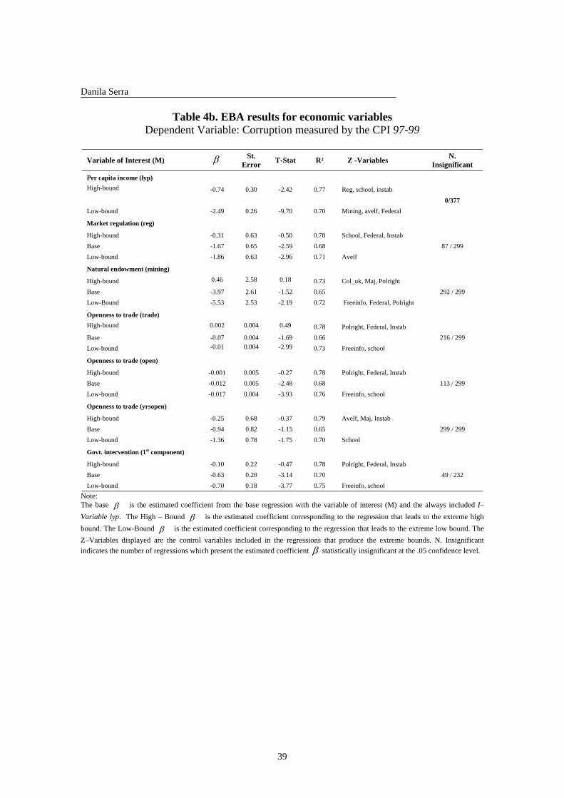
Danila Serra

39

Table 4b. EBA results for economic variables

Dependent Variable: Corruption measured by the CPI 97-99

Variable of Interest (M) β St. Error T-Stat R² Z -Variables N.

Insignificant

Per capita income (lyp) High-bound -0.74 0.30 -2.42 0.77 Reg, school, instab 0/377 Low-bound -2.49 0.26 -9.70 0.70 Mining, avelf, Federal

Market regulation (reg)

High-bound -0.31 0.63 -0.50 0.78 School, Federal, Instab Base -1.67 0.65 -2.59 0.68 87 / 299 Low-bound -1.86 0.63 -2.96 0.71 Avelf

Natural endowment (mining)

High-bound 0.46 2.58 0.18 0.73 Col_uk, Maj, Polright Base -3.97 2.61 -1.52 0.65 292 / 299 Low-Bound -5.53 2.53 -2.19 0.72 Freeinfo, Federal, Polright

Openness to trade (trade) High-bound 0.002 0.004 0.49 0.78 Polright, Federal, Instab Base -0.07 0.004 -1.69 0.66 216 / 299 Low-bound -0.01 0.004 -2.99 0.73 Freeinfo, school

Openness to trade (open)

High-bound -0.001 0.005 -0.27 0.78 Polright, Federal, Instab Base -0.012 0.005 -2.48 0.68 113 / 299 Low-bound -0.017 0.004 -3.93 0.76 Freeinfo, school

Openness to trade (yrsopen)

High-bound -0.25 0.68 -0.37 0.79 Avelf, Maj, Instab Base -0.94 0.82 -1.15 0.65 299 / 299 Low-bound -1.36 0.78 -1.75 0.70 School

Govt. intervention (1st component)

High-bound -0.10 0.22 -0.47 0.78 Polright, Federal, Instab Base -0.63 0.20 -3.14 0.70 49 / 232 Low-bound -0.70 0.18 -3.77 0.75 Freeinfo, school

Note: The base β is the estimated coefficient from the base regression with the variable of interest (M) and the always included I–Variable lyp. The High – Bound β is the estimated coefficient corresponding to the regression that leads to the extreme high bound. The Low-Bound β is the estimated coefficient corresponding to the regression that leads to the extreme low bound. The Z–Variables displayed are the control variables included in the regressions that produce the extreme bounds. N. Insignificant indicates the number of regressions which present the estimated coefficient β statistically insignificant at the .05 confidence level.

Danila Serra

40

Table 5b. EBA results for socio-cultural variables

Dependent Variable: Corruption measured by the CPI 97-99

Variable of Interest (M) β St. Error T-Stat R² Z -Variables N.

Insigniicant Protestant religion (prot80) High-bound -0.03 0.007 -3.83 0.82 School, Mining, Instab Base -0.04 0.007 -5.32 0.77 0 / 299 Low-bound -0.04 0.007 -5.24 0.77 Polright

British legal system (legor_uk)

High-bound -0.20 0.72 -0.29 0.75 Col_uk, School, Maj Base -1.37 0.39 -3.51 0.71 88 / 299 Low-bound -1.53 0.38 -4.00 0.74 Federal, Polright

Legor_uk (without col_uk)

High-bound -0.82 0.53 -1.54 0.75 School, Trade, Maj Base -1.37 0.39 -3.51 0.71 17 / 232 Low-Bound -1.53 0.38 -4.00 0.74 Polright, Federal

British colonial heritage (col_uk)

High-bound -0.49 0.67 -0.73 0.75 Reg, Trade, Legor_uk Base -1.45 0.41 -3.56 0.71 69 / 299 Low-Bound -1.12 0.66 -1.70 0.74 Legor_uk, Avelf, Freeinfo

Col_uk (without legor_uk)

High-bound -0.89 0.48 -1.85 0.75 Reg, Avelf, Maj Base -1.45 0.41 -3.56 0.71 0/ 232 Low-Bound -1.60 0.41 -3.86 0.72 Polright

Education (school)

High-bound 0.01 0.10 0.10 0.82 Reg, Prot80, Instab Base -0.29 0.11 -2.59 0.68 141 / 299 Low-Bound -0.34 0.12 -2.93 0.73 Polright, Mining, Trade

Ethno-linguistic fragmentation (Avelf)

High-bound -0.21 1.30 -0.20 0.71 Trade, legor_uk Base -1.63 0.98 -1.66 0.66 223 / 299 Low-bound -2.24 0.96 2.34 0.72 Polright, reg, federal

Ethno-linguistic fragmentation (Ethno)

High-bound 0.004 0.009 0.51 0.75 School, Legor_uk,Maj Base -0.01 0.009 -1.41 0.65 286 / 299 Low-bound -0.02 0.009 -2.02 0.71 Polright, trade federal

Note: The base β is the estimated coefficient from the base regression with the variable of interest (M) and the always included I–Variable, lyp. The High – Bound β is the estimated coefficient corresponding to the regression that leads to the extreme high bound. The Low-Bound β is the estimated coefficient corresponding to the regression that leads to the extreme low bound. The Z–Variables displayed are the control variables included in the regressions that produce the extreme bounds. N. Insignificant indicates the number of regressions which present the estimated coefficient β statistically insignificant at the .05 confidence level.

Danila Serra

41

Table 6b. EBA Results for Institutional Variables

Dependent Variable: Corruption measured by the CPI 97-99

Variable of Interest (M) β St. Error T-Stat R² Z-Variables N.

Insignificant

Political rights (polright) High-bound 0.50 0.21 2.30 0.73 Trade, Avelf, Maj Base 0.11 0.21 0.55 0.64 290 / 299 Low-bound -0.66 0.31 -2.11 0.72 Mining, Freeinfo, Federal Uninterrupted democracy (demo) High-bound -0.86 0.50 -1.71 0.83 Legor_uk, Prot80, Freeinfo Base -2.11 0.53 -3.99 0.72 0 / 299 Low-bound -2.44 0.54 -4.47 0.75 Mining, Polright

Freedom of information (freeinfo)

High-bound 0.05 0.02 2.60 0.72 Mining,Polright, Federal Base 0.02 0.01 1.57 0.65 203 / 299 Low-bound -0.002 0.01 -0.17 0.77 School, reg instab

Radio diffusion (radio)

High-bound 0.0008 0.0007 1.28 0.81 School, Prot80, Maj Base -0.001 0.0007 -2.16 0.67 223 / 299 Low-bound -0.002 0.0007 -2.82 0.72 Mining, federal, polright

Newspaper readership (newsp)

High-bound 0.0009 0.002 0.49 0.83 Prot80, Federal, Instab Base -0.005 0.002 -2.29 0.67 136 / 299 Low-bound -0.005 0.002 -2.39 0.69 Polright, mining

Television diffusion (tv)

High-bound 0.0006 0.001 0.45 0.82 School, Prot80, Instab

Base -0.003 0.002 -1.43 0.65 241 / 299 Low-bound -0.006 0.002 -2.94 0.73 Polright, mining, trade

Media (1st component)

High-bound 0.13 0.24 0.55 0.82 Prot80, school, Instab Base -0.66 0.22 -2.98 0.69 106 / 299 Low-bound -1.09 0.24 -4.43 0.77 Polright, Mining, Trade

Federalism (federal)

High-bound 1.29 0.51 2.51 0.72 Mining, Freeinfo, Polright Base 0.99 0.52 1.89 0.66 96 / 299 Low-bound 0.59 0.55 1.07 0.70 Reg, Trade, Polright

% vote on list (plist)

High-bound 1.04 0.44 2.33 0.70 Federal, Polright Base 0.79 0.44 1.81 0.66 225 / 299 Low-bound -0.44 0.44 1.01 0.81 Legor_uk, Polright, Instab

District magnitude (dismag)

High-bound 1.13 0.54 2.10 0.69 Federal, Polright Base 0.82 0.54 1.52 0.65 283 / 299 Low-bound -0.98 0.54 -1.81 0.82 Trade, Legor_uk, Instab

Majoritarian rule (maj)

High-bound 0.12 0.49 0.24 0.81 Legor_uk,Polright,Instab Base -1.16 0.41 -2.83 0.69 130 / 299 Low-bound -1.35 0.41 -3.30 0.72 Federal, Polright

Political instability (instab)

High-bound -0.88 0.32 -2.74 0.83 Trade, Prot80, Freeinfo Base -1.55 0.31 -5.06 0.76 0 / 232 Low-bound -1.77 0.37 -4.83 0.78 Trade, Federal, Polright

Table 7b. EBA results for interactive terms

Dependent Variable: Corruption measured by the CPI97-99 index

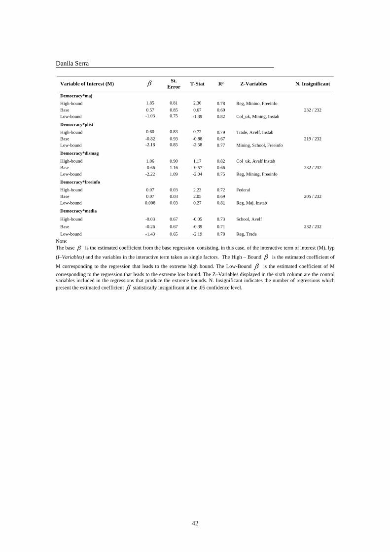
Danila Serra

42

Variable of Interest (M) β St.

Error T-Stat R² Z-Variables N. Insignificant

Democracy*maj

High-bound 1.85 0.81 2.30 0.78 Reg, Minino, Freeinfo Base 0.57 0.85 0.67 0.69 232 / 232 Low-bound -1.03 0.75 -1.39 0.82 Col_uk, Mining, Instab

Democracy*plist

High-bound 0.60 0.83 0.72 0.79 Trade, Avelf, Instab Base -0.82 0.93 -0.88 0.67 219 / 232 Low-bound -2.18 0.85 -2.58 0.77 Mining, School, Freeinfo

Democracy*dismag

High-bound 1.06 0.90 1.17 0.82 Col_uk, Avelf Instab Base -0.66 1.16 -0.57 0.66 232 / 232 Low-bound -2.22 1.09 -2.04 0.75 Reg, Mining, Freeinfo

Democracy*freeinfo

High-bound 0.07 0.03 2.23 0.72 Federal Base 0.07 0.03 2.05 0.69 205 / 232 Low-bound 0.008 0.03 0.27 0.81 Reg, Maj, Instab

Democracy*media

High-bound -0.03 0.67 -0.05 0.73 School, Avelf Base -0.26 0.67 -0.39 0.71 232 / 232 Low-bound -1.43 0.65 -2.19 0.78 Reg, Trade

Note: The base β is the estimated coefficient from the base regression consisting, in this case, of the interactive term of interest (M), lyp

(I–Variables) and the variables in the interactive term taken as single factors. The High – Bound β is the estimated coefficient of

M corresponding to the regression that leads to the extreme high bound. The Low-Bound β is the estimated coefficient of M corresponding to the regression that leads to the extreme low bound. The Z–Variables displayed in the sixth column are the control variables included in the regressions that produce the extreme bounds. N. Insignificant indicates the number of regressions which present the estimated coefficient β statistically insignificant at the .05 confidence level.