empirical approach to predict static capacity of drilled
TRANSCRIPT
5th World Congress on Civil, Structural, and Environmental Engineering (CSEE'20)
Lisbon, Portugal Virtual Conference – October 2020
Paper No. ICGRE 146
DOI: 10.11159/icgre20.146
ICGRE 146-1
Empirical Approach To Predict Static Capacity Of Drilled Shafts Based On High Strain Dynamic Pile Test Results
Ahmed Elgamal Mansoura Higher Institute of Engineering & Technology
Mansoura, Egypt
Abstract - The axial compression capacity of drilled shafts using full-scale tests has received the attention of many geotechnical
engineers. Regarding the extreme loads that large diameter shafts can resist, many cautions should be considered in the static load test
(SLT) application. The High Strain Dynamic Pile Test (HSDPT) is recommended as it propounds a substantial saving of time, cost, and
requirement of less space. Over the last decades, the signal matching analysis (e.g., Case Method, CAPWAP, and TNOWAVE) is
considered to be the most common procedure followed to predict the axial static response of piles based on HSDPT results. This paper
presents an empirical approach to predict the axial compression static capacity of drilled shafts based on HSDPT results. The ultimate
static pile capacity has estimated from HSDT results using a simplified formula that conveys the ultimate capacity to the pile set
occasioning from a hammer strike and not only the tip stratum properties but also other pile and soil/rock properties (shaft, tip soil, and
rock). Numerous well-documented full-scale tests and finite element models were used to develop and validate the suggested formula.
Keywords: High Strain Dynamic test, large diameter shaft, static pile capacity, finite element modelling, PLAXIS 3-D.
1. Introduction The traditional foundations are not appropriate to cope with revolutionary development in construction, which resulted
in structural elements that carry massive loads. Drilled shafts are most efficiently utilized where a strong bearing layer is
present. When placed to bear within or on a rock, extreme axial resistance can be achieved in a foundation with a small
footprint [1]. This is why large diameter drilled shafts have been frequently used than other deep foundations types. Also,
drilled shafts commonly utilized as an alternative solution in different subsurface conditions considering the mega-loads with
minimal settlement [1].
Owing to the long-time needed to perform, high cost, limitation of test space, and transportation difficulties, contractors
are seeking an alternative to conventional static load tests (SLTs) [2]. SLT is performed to verify the desired axial capacity
of pile structures. The methods of statement and data analysis procedure for SLT are well documented in the literature “[3]
[4]”. Recently, High Strain Dynamic Pile Test (HSDPT) adopted to supplement and in some cases, replace SLT. With more
advanced evaluation programs, the static bearing capacity determined from the results of HSDPT approximates the real static
bearing capacity, determined from SLT [5].
Calibrating HSDPT results with SLT for one or more initial piles reduce the time and number of required tests [6].
Regarding the same pile, performing an HSDPT after the fully mobilized SLT (test load = 1.5 times the pile static capacity)
may mislead the wave results [7]. Dynamic measurements were accurately recorded for each hammer blow by the two strain
transducers and two accelerometers that were fixed below the pile head, as shown in Fig. 1.
Consequently, the force (F) and velocity (V) records can be obtained as a function of time (t) by multiplying the pile
cross-sectional area (A) and the modulus of elasticity (E) by the measured strain (ε) and by integrating the recorded
acceleration (a) with time, respectively, as shown in Fig. 2.
The main concept of driving formulas and its modifications “[8] [9] [10] [11]”, is that the energy transferred to the pile
top equals to work done by the pile resistance for the observed pile set (S) in addition to the energy dissipated inside the pile
and within the soil during the pile impact using Eq. 1.
Eeff = eeffWhH = Qult(S + Sc) (1)

ICGRE 146-2
Where eeff is the effective energy transferred to the pile top which can also be calculated using Eq. 2[6], eeff is the
hammer efficiency that can be utilized 0.55 and 0.097 as an average value for driven and bored piles, respectively, for
dropped hammer, Qult is the ultimate pile static capacity and Sc is an empirical coefficient according to the pile elastic
compression during the impact load “[12] [13] [14] [15] [16]”.
Eeff = ∫ F(t) V(t) dtt
0
(2)
The value of the pile set can be obtained by integrating the velocity with time [6], see Fig. 2. The pile capacity can be
predicted from HSDPT after achieving a sufficient axial settlement that occurred during the impact event. A permanent net
penetration of as little as 2 mm per impact may indicate that adequate movement has occurred during the impact event to
mobilize the full capacity [6].
Fig. 1: Schematic sketch showing high strain dynamic testing of drilled shaft.
Fig. 2: Typical force and velocity schematic.

ICGRE 146-3
Achieving a successful HSDPT for a drilled shaft requires appropriate hammer details (i.e., weight, height, and caution
system) to cause sufficient pile movement. [6] recommends a hammer weight equal to 1% to 2% from the ultimate desired
pile capacity. [17] suggests values of Wh equal to 1%, 1.5%, and 2% from the desired ultimate pile capacity for piles rested
on a rock, friction piles, and drilled shafts with end bearing in coarse soils, respectively. The value of H should be varied
from 0.3m to 3m according to the same research. For test construction purposes, the light hammer weight with significant
height is more desirable than the heavy ones with low height [18].
Up to now, HSDPT is based on the practice, and the experience of one performed the test. The weight of the hammer
with corresponding height still to be determined. Some researches make focus on the confusing details of HSDPT to ensure
successful tests.[2] mentioned that dynamic tests will increasingly underestimate the results as the pile diameter and length
increase, possibly because insufficient energy is transmitted. Also, the correlation was best for piles in sand and gravel
compared with those in clay or in rock. [19] concluded that mobilized energy is a necessary requirement but an insufficient
condition. If so, it would be beneficial to know the energy levels or the impact value, which can trigger dynamic pile
settlement equal or similar to static pile settlement from SLT.
2. The concept of the study This research aims to create an empirical relationship between the hammer weight and corresponding height based on
the soil and pile properties considering the desired static capacity. Due to the few full-detailed historical data, Finite Element
Models (FEMs) that simulate SLT and HSDPT had been developed to fit out a well-established SLT/HSDPT results database.
Then formative a correlation between SLT and HSDPT to predict the axial compression capacity of large diameter shafts
based on soil, pile, and drop weight properties.
The drilled shafts studied had a range of diameters (D) from 800mm to 1500mm (broadly pile diameters) embedded in
different dense sandy soil layer (Dr = 30%, 60%, and 80%) with depth (Ls) and penetrated a limestone layer to a distance of
2D as shown in Fig. 3.
Fig. 3. The constitutive model used in the study.
The pile penetration distance (Lp) in the limestone layer was analysed to be 2D, 3D, and 4D, but the results found out
that the change of penetration depth has a slight effect on the pile behaviour under static and high strain dynamic tests. Table1
presents the pile's details modelled in FE analysis.

ICGRE 146-4
Table 1: Piles’ properties modeled in FE analysis.
D (mm)
800 1000 1200 1500 L
(m
) Ls (m)
20D 16 20 24 30
30D 24 30 36 45
40D 32 40 48 60
Lsock (m) 2D 1.6 2.0 2.4 3.0
In order to prepare the SLT-HSDPT results database, the FE procedure shall be verified to be used to model static and
high strain dynamic pile tests as cleared in the following sections.
3. Finite element modelling 3.1. Geometry and Boundary Conditions
PLAXIS 3-D 2018 is used to perform three-dimensional finite element models to simulate SLTs and HSDPTs,
respectively. Fig. 4 portrays the general layouts and soil meshing of the developed FEMs. For SLTs, the models extended to
50D and 30D in the horizontal and vertical directions, respectively, to release the effect of model boundary conditions. The
right and left edges were constrained from the horizontal movement only to avoid instability in the model analysis.
For the HSDPTs, the viscous boundaries were 150 D away from the pile center in each side in the horizontal plane (x-
y) and were applied to the bottom layer edge, which extended to 100D. This type of boundary was used to prevent errors
from being caused by the reflection effect of dynamic waves [20]. The bottom boundary of each model was constrained in
the horizontal and vertical directions.
Fig. 4: FE model geometry and boundary conditions for HSDPTs (PLAXIS 3-D).
3. 2. Meshing
3-D cubic volume shape was conducted around the pile, as shown in Fig. 5. The global mesh is medium to increase the
accuracy and save time, 3-D cubic volume shape was conducted around the pile with local refinement mesh (Rf = 0.1), as
shown in Fig. 6. Many trials were conducted to ensure that the model reaches to the accurate values.

ICGRE 146-5
Fig. 5: 3-D cubic volume shape.
Fig. 6: Mesh generation (Global + local refinement).
3.3. Soil and Pile Modelling
The 3-D tetrahedron elements were used to represent the soil for SLTs and HSDPTs. Different meshing sizes were
utilized to enhance the stress and settlement results. A zone of very fine mesh (with size 0.1m) was considered around and
below the pile. Progressively, the mesh size is increased until they reach the boundaries locations.
The hardening soil (HSM) model is used to define the isotropic soil layers. This model is an advanced double hardening
model (two surfaces represent the shear and compression yielding). The choice of this model is because of its ability to
capture the fundamental properties of soil material. HSM requires three different stiffnesses; (i) the secant modulus (E50ref)
from the standard drained triaxial test that can be assigned as a function of soil modulus of elasticity using Eq. 3, (ii) the
primary loading modulus (i.e., the tangent stiffness in oedometer loading) (Eoedref ) that equals to the value of E50
ref, (iii) the
unloading and reloading modulus (Eurref) which equals three times the value of E50
ref.
E50ref = E
2 − Rf
2
(3)

ICGRE 146-6
Where, Rf is a failure modification factor equals to 0.9 (recommended <1, [21]. One of the advantages of HSM is
that it considers the soil dilatancy angle (Ψ) which usually can be estimated from the soil internal friction angle (φ) (Ψ=
φ - 300) for soils that have a value of φ greater than 300. The pile was modelled as a linear-elastic material with mesh
elements as the surrounding soil (mesh size was taken as 0.1m). 3. 4. Interface Elements
The interaction between the soil/rock and the pile was defined using two elastic-perfectly plastic springs to simulate the
gapping and slipping. It should be noted that in calculating the interface element parameters, the value of R represents the
friction between soil and pile, which ranges from 0.6 to 1.0 according to pile material. The shear strength parameters at the
pile interface were taken as 𝟐 𝟑⁄ that of the neighboring soil. 3.5. Model Development
The non-linear analysis of SLTs was divided mainly into four construction stages, as shown in “Fig. 7”;
Stage 1 considers the initial stresses before pile installation.
Stage 2 Numerical instability is avoided by changing the soil in place of
pile-to-pile material and pile weight. All displacement results were cleared before applying the static load.
Stage 3 initiates by activating interface elements. In this stage, the static load was applied incrementally to simulate
the pile loading process as in the field testing.
The analysis of HSDPTs is a linear time history analysis to consider the impact load and contains two analysis
procedures. The first is an eigenvalue analysis type to determine the most effective time periods. The second analysis
procedure is the two modes that have the highest modal participation ratio are selected to perform the linear-time history
analysis ; this is the second analysis procedure.
Fig. 7: Stages of construction (static load).
3.6. HSDPT Simulation The impact load applied in the HSDPT could be simulated using a time history force function; see Fig. 2. The time
history function measured in the full-scale test performed by [13] was selected to produce the effective energy transferred to
the model piles head. Fig. 8 displays the time-history function used in the analysis of three different drops. It should be noted
that the forces in Fig. 8 were multiplied by constant factors (1, 2, 2.5, 3, 4, 5, and 6) to generate adequate energies to drive
the piles until they reach an acceptable displacement as previously illustrated. The HSDPT simulated model and its
construction stages show in Fig. 9.

ICGRE 146-7
Fig. 8: Typically applied time history functions for HSDPTs.
Fig. 9: Stages of construction (dynamic).
3.7. FEM Verification [13](Hussein et al. 1992) performed full-scale static and high strain dynamic load tests on a 660mm diameter concrete
pile with the equivalent pile properties presented in Table 2. The pile was free headed cast-in-place penetrated sandy and
clayey layers and rested on a weathered limestone with soil and rock properties shown in Table 3.
Table 2: Pile properties utilized for model calibration (after,[13]).
L (m) D (mm) γ (kN/m3) ν E (kPa)
13.70 660 25.67 0.2 2.4x10⁷
Table 3: soil/rock properties utilized for model calibration (after,[13]).
Layer Depth
(m)
Constitute
Model
Drainage
Type
γ Φ C
(kPa) ν
Eoed
(kN/m2)
E50
(kN/m2)
Eur
(kN/m2) (kN/m3) (degree)
Sand 0.0 -
9.15
Hardening
Soil model Drained 17 30 1 0.25 2500 2500 7500
Clay 9.15 –
11.0
Hardening
Soil model Undrained 18 1 50 0.3 12000 12000 36000
Limestone 11.0 –
40.0
Hardening
Soil model Drained 24 20 510.7 0.3 150000 150000 450000
The interface parameters were calculated as illustrated in section 3.3 and presented in Table 4. Fig. 10 showed the
measured and predicted pile-head load-displacement curves. A good agreement could be observed between the field results
and that obtained from the finite element model. The limestone Uniaxial Compressive Strength (UCS) is 1458.6 kPa [13].

ICGRE 146-8
Fig. 10: Measured and predicted load-displacement relationship for SLT validation.
The three dropped weights presented as time function forces in Fig. 11 were applied to the 3-D soil-pile model to validate
that the HSDPT can be modelled using PLAXIS 3-D 2018. No multiplier was applied to the three load functions (the same
in the field test). As reported by [13], the hammer had a weight of 97.5kN and dropped from heights equal to 0.92m, 2.14m,
and 2.44m. Fig. 11 portrayed the measured and predicted time-velocity relationship. Good agreements are observed for the
three different drops. The energies transferred to the pile top were calculated using Eq. 2 for the measured and the predicted
waves. The measured transferred energies were found to be 8.2 kN-m, 14.95 kN-m, and 25.5 kN-m for drops 1, 2, and 3,
respectively. The predicted ones were 10.8 kN-m, 17.85 kN-m, and 25.6 kN-m for the three drops, respectively.
(a) Drop 1 (0.92 m) (b) Drop 2 (2.14 m) (c) Drop 3 (2.44 m)
Fig. 11: Measured and predicted velocity versus time for HSDPT validation.
Table 4: FEM material properties.
Soil and rock properties
Density γ(kN/m3) φ (degree) UCS (MN/m2) ν* E* (kN/m2)
San
d Loose 17 30 - 0.25 15000
Medium dense 19 35 - 0.30 30000
Dense 21 40 - 0.35 60000
Limestone 22 28 100 0.30 10x106
Pile properties
Section Material D (mm) L (m) E (kPa) ν γ(kN/m3)
Circular Reinforced
concrete Table 1
2.2x10⁷ 0.2 25
* Values of soil Poisson`s ratio (ν) was assumed according to [22].

ICGRE 146-9
4. Database establishment (SLT-HSDPT database) Table 5 presents the soil, rock, and pile properties utilized in the FE analysis. It should be noted that the soil and rock
modulus of elasticity was estimated according to [22] and Eq. 3, respectively. The geometry, boundary condition, interface
parameters, and analysis stages were the same as illustrated in sections 3.1 to 3.4. The three load functions presented in
section 3.5 were utilized by applying multiplier factors to achieve an adequate displacement (i.e., >2mm).
The finite element analysis results are presented in Table 5 for each pile diameter from 800mm to 1500mm. All analysis
models were performed based on test data presented by [13], so the value of eeff can be used equal to 0.097.
As previously discussed, the eigenvalue analysis type was performed on each FE model to obtain the most critical modes
of shape. Choose the maximum of two-controlling time periods (modes of shape); the HSDPT results can be estimated from
the FE time-history analysis. The SLTs were simulated using PLAXIS 3-D 2018.[3] is the method was applied to the SLT
model results to predict the static capacity (Q10%).
Table 5: Inputs and outputs of FEMs.
D =
80
0 m
m
Lp (m) 17.6 25.6 33.6
Ls (m) 16 24 32
Lsock (m) 1.6 1.6 1.6
Dr (%) 30 60 80 30 60 80 30 60 80
UCS (MN/m2) 1.4 1.4 1.4 1.4 1.4 1.4 1.4 1.4 1.4
H (m) 4.8 2.8 2.2 4.3 1.6 1.2 3.2 1.5 1.0
Wh (kN) 154 170 186 334 370 406 436 458 506
S (mm) 3.51 3.46 3.42 4.89 4.75 4.63 6.41 5.9 5.45
Qult (kN)×104 0.84 1.58 2.15 1.40 4.2 5.98 3 6.90 10.98
D =
10
00
mm
Lp (m) 22 32 42
Ls (m) 20 30 40
Lsock (m) 2 2 2
Dr (%) 30 60 80 30 60 80 30 60 80
UCS (MN/m2) 1.4 1.4 1.4 1.4 1.4 1.4 1.4 1.4 1.4
H (m) 3 2.7 1.85 1.75 1.25 0.9 0.77 0.55 0.72
Wh (kN) 248 283 320 653 723 794 853 947 1041
S (mm) 2.7 2.65 2.59 6.0 5.76 5.53 8.07 7.4 6.3
Qult (kN)×104 2.12 2.54 4.03 6.80 10.23 15.13 19.23 28.62 21.66
D =
12
00
mm
Lp (m) 26 38 50
Ls (m) 24 36 48
Lsock (m) 2 2 2
Dr (%) 30 60 80 30 60 80 30 60 80
UCS (MN/m2) 1.4 1.4 1.4 1.4 1.4 1.4 1.4 1.4 1.4
H (m) 2.6 2.3 1.6 1.7 1.3 1.1 1 0.8 0.6
Wh (kN) 1125 1253 1480 1820 1950 2250 2430 2800 3150
S (mm) 2.27 2.21 2.15 3.36 3.15 3.0 4.42 4.0 3.72
Qult (kN)×104 5.79 7.0 11.1 11.9 16.3 20.7 24.76 33.07 47.0
D =
15
00
mm
Lp (m) 33 48 63
Ls (m) 30 45 60
Lsock (m) 3 3 3
Dr (%) 30 60 80 30 60 80 30 60 80
UCS (MN/m2) 1.4 1.4 1.4 1.4 1.4 1.4 1.4 1.4 1.4
H (m) 2.1 2.0 1.45 1.9 1.4 1.0 1.4 1.0 0.73
Wh (kN) 1256 1433 1619 1918 2222 2545 2645 3101 3591
S (mm) 0.97 0.966 0.96 2.79 2.60 2.42 3.52 3.23 2.98
Qult (kN)×104 8.08 9.13 13.70 13.61 20.04 30.21 22.3 34.04 50.27
ICGRE 146-10
5. Results discussion The results of SLT and HSDPT models have been analysed , and it was found that there is an empirical relationship
eq. 4 between static capacity (kN) of drilled shaft piles that penetrate soil/rock profiles as shown in Fig. 3 with the following
variables:
1. Wh , the weight of the hammer, kN;
2. H, corresponding drop height, m;
3. eeff, the efficiency of drop;
4. Dr, the relative density of the sandy layer;
5. D, pile diameter, mm;
6. Lsock, socket length, m;
7. LP, pile penetration distance in the limestone layer, m;
8. S, pile settlement, mm;
9. UCS, uniaxial compression strength of rock, MN/m2;
10. Ls, depth of sandy layer, m; The pile penetration distance (Lp) in the limestone layer
11. σv0` , effective stresses through pile shaft, MN/m2,
Qult = 1.30 + 0.23(eeff Wh H × 108)0.44
(eeff Wh H
WpLp)
1.51
exp (−0.05
Lp [
DrLs
100 +UCS Lsock
σvo, ]) (
SD)
−0.26 (D
Lp)
1.63
(4)
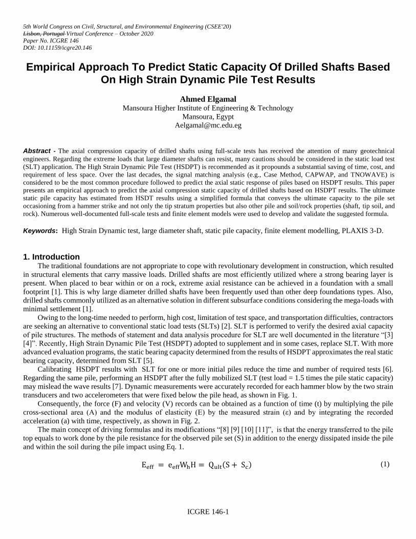
It seems there is a relationship between measured and predicated static pile capacity for different pile diameters, as
shown in Fig. (12). By using this relation no need to calibrate HSDPT with full-scale SLT. It can make safe more money,
time, and effort.
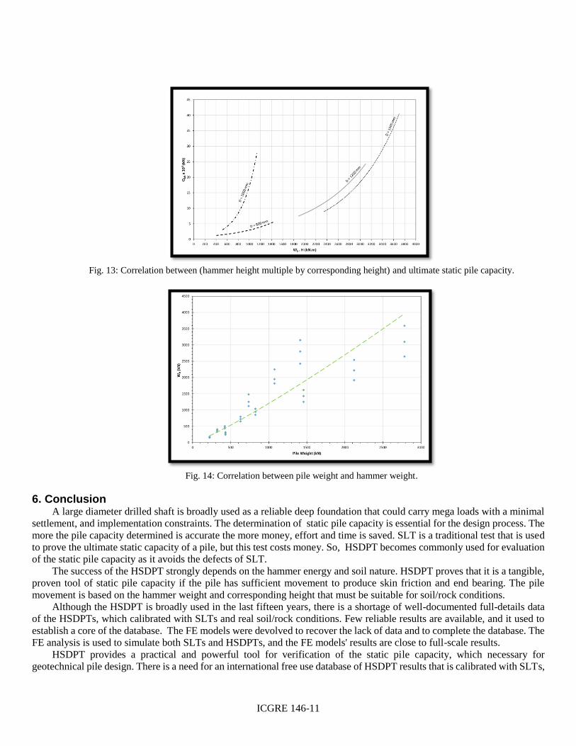
An increasing relationship between pile weight and the weight of the hammer is shown in Fig. (14). This relationship
is expected, especially in drilled shat, as the weight of the hammer produces a force that causes a pile movement, and this
force supposed to be close to the weight of the pile.
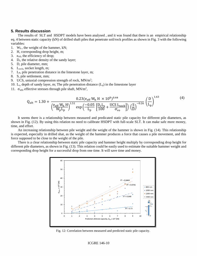
There is a clear relationship between static pile capacity and hammer height multiply by corresponding drop height for
different pile diameters, as shown in Fig. (13). This relation could be easily used to estimate the suitable hammer weight and
corresponding drop height for a successful drop from one time. It will save time and money.
Fig. 12: Correlation between measured and predicted static pile capacity.
ICGRE 146-11
Fig. 13: Correlation between (hammer height multiple by corresponding height) and ultimate static pile capacity.
Fig. 14: Correlation between pile weight and hammer weight.
6. Conclusion A large diameter drilled shaft is broadly used as a reliable deep foundation that could carry mega loads with a minimal
settlement, and implementation constraints. The determination of static pile capacity is essential for the design process. The
more the pile capacity determined is accurate the more money, effort and time is saved. SLT is a traditional test that is used
to prove the ultimate static capacity of a pile, but this test costs money. So, HSDPT becomes commonly used for evaluation
of the static pile capacity as it avoids the defects of SLT.
The success of the HSDPT strongly depends on the hammer energy and soil nature. HSDPT proves that it is a tangible,
proven tool of static pile capacity if the pile has sufficient movement to produce skin friction and end bearing. The pile
movement is based on the hammer weight and corresponding height that must be suitable for soil/rock conditions.
Although the HSDPT is broadly used in the last fifteen years, there is a shortage of well-documented full-details data
of the HSDPTs, which calibrated with SLTs and real soil/rock conditions. Few reliable results are available, and it used to
establish a core of the database. The FE models were devolved to recover the lack of data and to complete the database. The
FE analysis is used to simulate both SLTs and HSDPTs, and the FE models' results are close to full-scale results.
HSDPT provides a practical and powerful tool for verification of the static pile capacity, which necessary for
geotechnical pile design. There is a need for an international free use database of HSDPT results that is calibrated with SLTs,

ICGRE 146-12
to change the test from being experience-based into casual user based. This research will contribute to this attitude. More
studies are needed to cover all soil/rock conditions with reliable data.
References [1] O’Neill, M. W., and Reese, L. C. (1999). “Drilled shaft: construction procedures and design methods.” FHWA Report
No. IF-99-025.
[2] Long, M. (2007). “ Comparing dynamic and static test results of bored piles.” Proceeding of the Institution of Civil
Engineering, Geotechnical Engineering 160, January 2007, Issue GEI, Pages 43-94.
[3] Davisson, M. T. (1972). “High capacity piles.” Proc., Lect. Series on Innovation in Found. Const., ASCE, Illinois Section,
Chicago, p. 52.
[4] Fellenius, B. H. (1980). “The analysis of results from routine pile load tests. Ground Engineering.”, London, Vol. 13, No.
6, pp. 19 – 31.
[5] Schell, P., Szilvagyi, L., and Wolf, A. (2015). “ Case study of a static-dynamic pile load test program in Hungary.”,
Proceedings of the XVI ECSMGE, Geotechnical Engineering for Infrastructure and development,
DOI:101680/ecsmge.60678.
[6] ASTM (2017). “Standard test method for high-strain dynamic test,” Designation: D4945 – 17.
[7] Briaud, J.-L., Ballouz, M., and Nasr, G. (2000). “Static capacity prediction by dynamic methods for three bored piles.”,
ASCE, Journal of Geotechnical and Geoenvironmental Engineering, Vol. 126, No. 7, July 2000, Paper No. 17460.
[8] Gates, M. (1957). “Empirical formula for predicting pile bearing capacity.” ASCE March 1957, vol. 27,pp. 65-66.
[9] ENR (1965). "Michigan pile test program test results are released," Michigan State Highway Commission, March 1965,
Eng. News-Record, pp. 26-28, 33-34.
[10] Olson, R., and Flaate, K. (1967). “Pile-driving formulas for friction piles in sand.”, Journal of Soil Mechanics &
Foundations Division, vol. 92, pp. 279-296.
[11] Salgado, R., Zhang, Y. Abou-Jaoude, G., Loukidis, D., and Bisht, V. (2017). “Pile driving formulas based on pile wave
equation analyses.”, Computers and Geotechnics, Volume 81, January 2017, Pages 307-32.
[12] PC, L., and Broms, B. (1990). “Influence of pile driving hammer performance on driving criteria.” Geotech Engineering
, vol. 21,1990, pp. 63-69.
[13] Hussein, M., Townsend, F., Rausche, F., and LIKINS, G. (1992). “Dynamic testing of drilled shafts.” Transportation
Research Record, 1336.
[14] Allen, T. (2005). “Development of the WSDOT Pile Driving Formula and its calibration for Load and Resistance Factor
Design (LRFD),” WA-RD 610.1., Final research report, March 2005,Washington State Department of Transportation.
[15] Lam, J. (2007). “Termination criteria for high-capacity jacked and driven steel H-piles in Hong Kong,” Ph.D. thesis,
The University of Hong Kong, Hong Kong, China.
[16] Mostafa, Y. (2011). “Onshore and offshore pile installation in dense soils.” Journal of American Science, 2011;7(7),pp.
549–563.
[17] Robinson, B., Rausche, F., Likins, G., and Ealy, C. (2002). “Dynamic Load Testing of Drilled Shafts at National
Geotechnical Experimentation Sites.” Deep Foundations 2002: An International Perspective on Theory Design,
Construction, and Performance.
[18] Hussein, M., Likins, G., and Rausche, F. (1996). “Selection of a hammer for high-strain dynamic testing of cast-in-place
shafts.” Fifth International Conference on the Application of Stress-Wave Theory to Piles, Orlando, Florida, USA.
[19] Svinkin, MR (2019). “Sensible determination of pile capacity by dynamic methods.”, Geotechnical research 6(1):52-
67, https://doi.org/10.1680/jgere.18.00032.
[20] Lysmer, J., and Waas, G. (1972). “Shear waves in plane infinite structures.”, ASCE, Journal of Engineering Mechanics,
Feb. 1972, vol. 98, pp. 85 -105.
[21] PLAXIS 3-D (2018). “ PLAXIS 3-D Manual”.
[22] Bowles, J.E. (1996) “Foundation analysis and design.”, 5th Edition, The McGraw-Hill Companies, Inc., New York.