emitter localization and compressed sensing: a low cost

Rose-Hulman Institute of TechnologyRose-Hulman Scholar

Graduate Theses - Engineering Management Graduate Theses

Spring 5-2014

Emitter Localization and Compressed Sensing: ALow Cost Design Using Coarse Direction FindingAntennasAndrew Raymond WagnerRose-Hulman Institute of Technology, [email protected]

Follow this and additional works at: http://scholar.rose-hulman.edu/engineering_management_grad_theses

Part of the Computational Engineering Commons

This Thesis is brought to you for free and open access by the Graduate Theses at Rose-Hulman Scholar. It has been accepted for inclusion in GraduateTheses - Engineering Management by an authorized administrator of Rose-Hulman Scholar. For more information, please contact [email protected].

Recommended CitationWagner, Andrew Raymond, "Emitter Localization and Compressed Sensing: A Low Cost Design Using Coarse Direction FindingAntennas" (2014). Graduate Theses - Engineering Management. Paper 1.

http://scholar.rose-hulman.edu?utm_source=scholar.rose-hulman.edu%2Fengineering_management_grad_theses%2F1&utm_medium=PDF&utm_campaign=PDFCoverPages

http://scholar.rose-hulman.edu/engineering_management_grad_theses?utm_source=scholar.rose-hulman.edu%2Fengineering_management_grad_theses%2F1&utm_medium=PDF&utm_campaign=PDFCoverPages

http://scholar.rose-hulman.edu/graduate_theses?utm_source=scholar.rose-hulman.edu%2Fengineering_management_grad_theses%2F1&utm_medium=PDF&utm_campaign=PDFCoverPages



http://network.bepress.com/hgg/discipline/311?utm_source=scholar.rose-hulman.edu%2Fengineering_management_grad_theses%2F1&utm_medium=PDF&utm_campaign=PDFCoverPages

http://scholar.rose-hulman.edu/engineering_management_grad_theses/1?utm_source=scholar.rose-hulman.edu%2Fengineering_management_grad_theses%2F1&utm_medium=PDF&utm_campaign=PDFCoverPages

mailto:[email protected]

mailto:[email protected]

Emitter Localization and Compressed Sensing:

A Low Cost Design Using Coarse Direction Finding Antennas

A Thesis

Submitted to the Faculty

Of

Rose-Hulman Institute of Technology

By

Andrew Raymond Wagner

In Partial Fulfillment of the Requirements for the Degree

Of

Master of Science in Systems Engineering & Management (International Program)

May 2014

© 2014 Andrew Raymond Wagner

ABSTRACT

Wagner, Andrew Raymond

M.S.S.E.M.I

Rose-Hulman Institute of Technology

May 2014

Emitter Localization and Compressed Sensing: A Low Cost Design Using Coarse Direction Finding Antennas

Thesis Advisor: Dr. Deborah Walter

Research has been conducted to determine the location of uncooperative radio-frequency

(RF) emitters, using low cost sensors employing broadband, low directivity antennas.

Comparably lowered accuracy and longer response time may be appropriate trade-offs for size,

weight, and power (SWAP). These sensors can then be deployed on numerous testbeds, and

algorithms may take advantage of the reconfigurable, distributive network of sensors to precisely

determine the location. To conduct this research, a network of three reconfigurable sensors,

equipped for emitting and receiving RF signals, was designed based on Universal Software

Radio Peripheral (USRP™) technology. This thesis details the experiments conducted and the

results obtained to develop accurate models of the receiving sensors and to validate the emitter

location algorithm.

DEDICATION

I would like to first thank all of my family for their support as I worked towards

completing my master’s degree. My mother was especially supportive, not only throughout

graduate school, but throughout my entire education to instill a strong work ethic which has

made me persistent and hard-working with everything I do. She is truly a valuable asset to my

life and for this, I want to thank her.

Another thank you goes to the rest of my family, extended family, and friends who

provided me motivation especially when it was needed most throughout college. I am thankful

for all of the encouragement I have received from high school friends, college friends, and those

I have met while studying and traveling abroad.

I also owe my coworkers a sign of appreciation to thank them for the support I received

while in the process of completing my thesis. Having the opportunity to work with several

people who have received either a master’s degree or a doctorate has allowed me to look to them

for both guidance in my research and support.

ACKNOWLEDGEMENTS

I would first like to thank Dr. Deborah Walter for all of her help in completing this thesis.

Without her assistance, I could not imagine accomplishing this feat. Her knowledge of the

subject, thorough critiquing, and patience in dealing with my work progress was beneficial

towards guiding me to a completed thesis. She served as a valuable Thesis Advisor.

I would also like to thank Dr. Daniel Moore who was always available to lend advice not

only on my thesis, but throughout my graduate school program. I also extend my gratitude to my

German advisors from Hochschule Ulm, Prof. Dr. Dirk Bank and Prof. Dr. Roland Münzner.

This Thesis Advisory Committee is greatly appreciated.

Another thank you is extended to the senior design members at Rose-Hulman Institute of

Technology, as well as those students who took the time out of their busy schedules to help me

collect data for this research. I am greatly appreciative of all those students at Rose-Hulman who

are always there to help out others when possible.

I would finally like to thank all of those at Wright-Patterson Air Force Base and the

American Society of Engineering Education for the help I received while conducting research.

This thesis would not be completed without the guidance and testing equipment that was

provided to me from these groups.

ii

TABLE OF CONTENTS

Contents LIST OF FIGURES ............................................................................................................... iv LIST OF TABLES ................................................................................................................. vi LIST OF ABBREVIATIONS .............................................................................................. vii

1. INTRODUCTION..............................................................................................................1 1.1 CHAPTER OVERVIEW ...................................................................................1 1.2 PROBLEM STATEMENT ................................................................................1 1.3 RESEARCH OBJECTIVES, HYPOTHESIS, & QUESTIONS ....................2 1.4 PREVIEW ...........................................................................................................3

2. BACKGROUND ................................................................................................................4 2.1 CHAPTER OVERVIEW ...................................................................................4 2.2 THE MOBILE SENSOR TESTBED ................................................................4 2.3 GEOLOCATION/LOCALIZATION ...............................................................7 2.4 ELECTRONIC WARFARE ..............................................................................8 2.5 COMPRESSED SENSING ................................................................................9 2.6 CURRENT RESEARCH & APPLICATION AREAS ..................................11 2.7 SUMMARY .......................................................................................................12

3. OBJECTIVE 1 – MODEL/CALIBRATION TESTS ...................................................13 3.1 CHAPTER OVERVIEW .................................................................................13 3.2 PROBLEM DEFINITION ...............................................................................13 3.3 DEFINITION OF TERMS...............................................................................13 3.4 RSS VS. DISTANCE TEST .............................................................................14 3.5 ANTENNA TEST PATTERN .........................................................................19 3.6 INDOOR RANGE TESTING ..........................................................................22 3.7 RANGE GATING .............................................................................................26 3.8 SUMMARY .......................................................................................................30

4. OBJECTIVE 2 – FEASIBILITY ....................................................................................31 4.1 CHAPTER OVERVIEW .................................................................................31 4.2 OUTDOOR RANGE TESTING/TEST SCENARIOS ..................................31 4.3 GOALS AND HYPOTHESES .........................................................................32 4.4 LOCALIZATION TECHNIQUES .................................................................33

4.4.1 HOW OTHERS DO IT ...............................................................33 4.4.2 COMPRESSED SENSING .........................................................34

4.5 TEST SCENARIO #1 ........................................................................................35 4.6 TEST SCENARIO #1 RESULTS .....................................................................36 4.7 TEST SCENARIO #2 ........................................................................................39 4.8 TEST SCENARIO #2 RESULTS .....................................................................40 4.9 SUMMARY ........................................................................................................42

5. CONCLUSIONS AND RECOMMENDATIONS .........................................................44 5.1 CHAPTER OVERVIEW .................................................................................44 5.2 RESEARCH CONCLUSIONS ........................................................................44 5.3 RESEARCH SIGNIFICANCE ........................................................................49 5.4 FUTURE RESEARCH RECOMMENDATIONS .........................................49

iii

5.5 SUMMARY .......................................................................................................54 LIST OF REFERENCES ......................................................................................................55 APPENDIX A .........................................................................................................................57

iv

LIST OF FIGURES

Figure Page

Figure 2.1: Sensor Testbed Configurations ...............................................................................5

Figure 2.2: Emitter Testbed (left) and Receiver Testbed (right) ...............................................6

Figure 3.1: RSS vs. Distance Test Setup for Outdoor Experimentation ..................................15

Figure 3.2: RSS vs. Distance Outdoor Measurement Results & Piecewise Linear Fit ...........16

Figure 3.3: RSS vs. Distance Test Setup for Indoor Range .....................................................17

Figure 3.4: RSS vs. Distance Indoor Measurement Results ....................................................18

Figure 3.5: Receiver Antenna Pattern, Outdoor Measurement Results ...................................21

Figure 3.6: Receiver Antenna Pattern Test Setup for Indoor Range .......................................23

Figure 3.7: Receiver Antenna Pattern, Indoor Measurement Results & Model Data ..............25

Figure 3.8: Calibrated Gain vs. Frequency for Range Gating .................................................28

Figure 3.9: Calibrated Gain vs. Rotation Angle for Range Gating ..........................................29

Figure 4.1: Test Scenario Layout for Outdoor Experimentation .............................................32

Figure 4.2: (a) Emitter Location Unknown (left) and (b) Localized Emitter Location (right)

for Test Scenario #1 ...........................................................................................................35

Figure 4.3: Test Scenario #1 Path with “Error Reported” .......................................................37

Figure 4.4: (a) Emitter Location Unknown (left) and (b) Localized Emitter Location (right)

for Test Scenario #2 ...........................................................................................................40

Figure 4.5: Test Scenario #2 Path with “Error Reported” .......................................................41

Figure 5.1: RSS vs. Distance Measurement with AC Power, Log-Periodic Antenna .............45

v

Figure 5.2: RSS vs. Distance Measurement with AC Power, Omnidirectional Antenna ........46

Figure 5.3: Diagram of Signal Reflections from Ground Plane ..............................................47

Figure 5.4: RSS vs. Distance Measurement for Arena Testing ...............................................48

Figure 5.5: Ground Bounce Null Calculation ..........................................................................51

Figure 5.6: Ground Bounce Propagation .................................................................................52

vi

LIST OF TABLES

Table Page

Table 3.1: RSS vs. Distance Piecewise Linear Fit Values for Outdoor Experimentation of

Figure 3.2 ...........................................................................................................................19

Table 4.1: Simulated vs. Measured RSS Values for Test Scenario #1 ....................................38

Table 4.2: Simulated vs. Measured RSS Values for Test Scenario #2 ....................................42

vii

LIST OF ABBREVIATIONS

TDOA Time Difference of Arrival

AOA Angle of Arrival

RSS Received Signal Strength

CS Compressed Sensing

EW Electronic Warfare

MATLAB Matrix Laboratory

USRP Universal Software Radio Peripheral

SDR Software Defined Radio

ISM Industrial, Scientific, and Medical

GPS Global Positioning System

TOA Time of Arrival

ES Electronic Support

EP Electronic Self-Protection

EA Electronic Attack

UAV Unmanned Aerial Vehicle

viii

CCD Charge-Coupled Device

CMOS Complementary Metal-Oxide Semiconductor

FDOA Frequency Difference of Arrival

1

1. INTRODUCTION

1.1 Chapter Overview

This chapter presents a description of the problem and a need for the research. It also

presents the research hypothesis, as well as the objective tasks used in analyzing the hypothesis.

1.2 Problem Statement

The localization of radio-frequency signals emitted is an issue faced in many

applications, including those relating to safety, emergency, and security. Completing the task of

localizing an emitter of a particular signal requires expensive and calibrated equipment. These

pieces of equipment help to perform algorithm techniques which include, but are not limited to,

time difference of arrival (TDOA) and angle of arrival (AOA). For measuring the time difference

of a signal received at multiple receivers, each individual receiver needs to be synchronized

precisely in a way that can be quite difficult so that data collection can be performed

synchronously. If the angle of arrival technique were used, an expensive, highly directive

receiving antenna would need to be implemented which had a narrow beam width (for example,

1° or less).

An alternative approach to the expensive and highly complex localization systems is

presented in this research. The focus of this approach is on measuring the received signal

strength (RSS) as measured by a single receiver. The problem of using the RSS measurement, as

posed by [1], is that the values can be highly inaccurate and thus unreliable for use in localizing a

signal source. With the information contained within this research, a new approach using RSS

2

measurements and a mathematical process point towards a possible valid solution with

inexpensive equipment that is able to localize an emitter with some degree of accuracy.

The question is whether it is possible to develop a low cost solution using coarse

direction finding antennas. From a broad point of view, this research is intended to prove it is

possible to localize some number of emitters without compromising accuracy or precision as

compared with other localization techniques.

The benefits of correctly localizing a signal of interest with an economical low cost

solution cannot be entirely determined at this point. Situations where this technology would be

helpful range from uses in electronic warfare (EW) for the military to finding lost fire fighters or

miners in the event of a structural collapse or other emergency. A cheap solution to locate a

signal will surely spur advances in many sectors for personal, commercial, industrial, and

military use.

1.3 Research Objectives, Hypothesis, & Questions

The objective of this research is to test the hypothesis that a sensor network employing

low accuracy, low cost, coarse direction finding sensors is able to locate a given signal of interest

without compromising precision or accuracy. To test this hypothesis, a low cost mobile testbed

consisting of a number of sensors was used. Because the sensors of the system that is being

tested are not highly precise and accurate, an alternative approach other than the expensive

equipment paired with TDOA, AOA, etc. to analyze the data needed to be used. A method called

compressed sensing (CS) was introduced for calculating the emitter locations with the sensor

system. This approach assumes a sparse solution exists and that there are only a handful of

3

possible emitters, since it is not practical to measure a countless number of emitters. To test the

research hypothesis, two main objectives were established:

• Model the sensor system

• Prove the feasibility of the sensor system through the use of case studies

The first objective, modeling the sensor system, established calibration data. This

calibration data would be used to model the sensor system in a MATLAB [2] simulation which

was helpful in determining how the system might work in actual testing. The next objective of

proving the feasibility of the system through case studies resulted from the MATLAB

simulation. With this objective, tests were conducted outdoors with the testbeds to mimic how

UAVs might randomly navigate in a given space while measuring for the presence of some

number of emitters. The results from this testing could then be compared with the results from

the simulation.

1.4 Preview

Chapter 2: Background discusses in more detail the mobile testbed used for testing the

hypothesis. Related topics with the research are also discussed. Chapter 3: Objective 1 –

Model/Calibration Tests reviews the calibration tests and the results which were used in

modeling the sensor system. Chapter 4: Objective 2 - Feasibility provides results and analysis

from the case studies which prove the feasibility of the sensor system. Lastly, Chapter 5:

Conclusions and Recommendations provides a summary of the results of the research, their

significance as they pertain to the hypothesis, and recommendations for future work on the

capability of localizing a given emitted signal of interest.

4

2. BACKGROUND


In this chapter, the mobile testbed used for testing the hypothesis is discussed in more

detail. Related topics to the research are defined and current research and applications related to

this research are discussed. Throughout this chapter, and the rest of this thesis, the term testbed is

used to refer to a single mobile platform such as the receiver and emitter platforms. The term

system is generally used to collectively group the testbeds together.

2.2 The Mobile Sensor Testbed

The sensor testbeds for the research were developed by an undergraduate team at Rose-

Hulman Institute of Technology during the 2012/2013 academic year. The team designed and

built a sensor network with three guiding principles. The testbeds each needed to be mobile so

the sensor testbeds are mounted to wheel bases. The testbeds also needed to be reconfigurable.

The transmitting and receiving antennas of the testbeds are all controlled by an embedded

Universal Software Radio Peripheral (USRP). The remaining sensors, the communication with

the USRP, and the communication through Wi-Fi are all controlled by a BeagleBone processor.

Figure 2.1 shows the configuration of the sensors which demonstrates how all of the internal

communication works. Creating a relatively inexpensive solution was the third principle that

guided the design of the sensor system. Compared with highly capable and highly directive

antenna units currently used for geolocation purposes, the three testbeds used in the research

work could be replicated for a combined cost of under $6,000 in addition to the time associated

with building the system.

5

Figure 2.1: Sensor Testbed Configurations [3]

The sensor system that the research involved consisted of three nodes (testbeds): one

functioning as an emitter, one functioning as a receiver, and one which is capable of functioning

as either an emitting or a receiving testbed. It is the ability of reconfiguring the testbeds which

allows the third testbed to function as an emitter or a receiver, whichever is desirable for testing.

The only physical modification for this conversion is the altering of the antenna to be used, using

a simple omnidirectional antenna for the emitter testbed and a direction-sensitive log-periodic

antenna for the receiver testbed. One emitter testbed and one receiver testbed are shown in

Figure 2.2.

6

Figure 2.2: Emitter Testbed (left) and Receiver Testbed (right)

The USRP is a software defined radio (SDR) manufactured by Ettus Research. A

software defined radio is similar to a communication radio in that it can transmit or receive a

signal. The “software” term implies that the signal modulation and the carrier frequency are

software generated. One of the main reasons SDR’s are useful and practical in research like this

is because very minimal hardware modifications are required for them.

The operating frequency which is transmitted by the emitter testbed is currently 925

MHz, a frequency which falls within the industrial, scientific, and medical (ISM) band, a radio-

frequency band set aside for industrial, scientific, or medical purposes and allows for other low

power usage. This frequency can be altered depending on the testing environment. The USRP

was equipped with the RFX900 daughter card which allows a frequency of 750 – 1050 MHz to

be used, although other daughter cards may be used in place of the RFX900 which are capable of

use for some spectrum range between DC and 6 GHz [4].

7

All of the communication between the testbeds is done through a closed, private Wi-Fi

network alongside the base station. The base station is the user’s computer which is running

MATLAB. MATLAB is responsible for fetching data from each of the sensor testbeds. This data

includes information such as the longitude and latitude from the global positioning system

(GPS), the heading from the digital compass, the received signal strength (RSS, only from the

receiver testbeds) from the log-periodic antenna via the USRP, and a time stamp from an internal

clock to list the fetched data in chronological order when the data is listed in a text file.

2.3 Geolocation/Localization

Geolocation, similar to the global positioning system (GPS), deals with the localization of

objects in the real world. Sensors can be used to measure a specified frequency which results in

information such as the received signal strength (RSS), angle of arrival (AOA), time of arrival

(TOA), time difference of arrival (TDOA), and others, which can be used for the techniques and

algorithms mentioned in Section 4.4: Localization Techniques. Based on the configurations of

the sensors, a location can be calculated for the origin of a radio-frequency signal emission.

For this research, the RSS information is the only information being actively measured.

From the RSS value, and based on information about the log-periodic antenna of the receiving

testbed which helps produce AOA information, a desired location can be calculated. The result

of this calculation through multiple measurements can improve the localization of the signal

origin. The geolocation of an object or signal does not have to rely on only a single piece of

information, and it is common to use multiple pieces to verify and validate a location. With the

sensor system used in this research, multiple calibration tests were established to understand the

specifications of how the RSS value would be measured in a realistic setting. Explained more in

8

Chapter 3: Objective 1 – Model/Calibration Tests, the first objective of the research deals with

creating a model of the sensor system (more specifically the log-periodic antenna used with the

receiver testbed) in order to best characterize how an individual RSS value would affect the

geolocation of a signal.

2.4 Electronic Warfare

Electronic warfare (EW) is used by the military to advance diplomatic and economic

objectives or hinder undesired consequences. It refers to the use of the electromagnetic spectrum

to deny spectrum usage to the adversary, protect friendly usage of the spectrum, and to use the

spectrum for sensing and surveillance. The military employs usage of the electromagnetic

spectrum through radio communication; surveillance; sensing for detecting friendly, neutral, and

enemy forces; and remote wireless control [5]. Uses of EW are prevalent throughout a combat

situation in order to aid the Warfighter. The functions of EW are broken into three related

categories: electronic support (ES), electronic self-protection (EP), and electronic attack (EA)

[6]. ES helps to gather information about a potential threat to analyze ways to perform counter-

measure maneuvers. From analyzing the possible threats, the Warfighter employs EP to

manipulate bands of the spectrum to control conflicts and defend from enemy attacks. EA is

applied to then counter-attack a non-cooperative threat.

Use of EW attacks and counter-attacks has been around since the origination of radio

technology when the best technique was to jam a radio-frequency signal with noise. Now the

fight of the spectrum has evolved to incorporate uses in the air, at sea and underwater, on land,

and in space. Technology has evolved to better detect threats while also being able to operate

9

undetected. The electronic warfare battle is continuously progressing towards developing the

latest and greatest counter-measure to any known spectrum attack.

2.5 Compressed Sensing

This section deals with a broad overview of compressed sensing and relates how it can be

used with the objectives of this research. Compressed sensing (CS), a theory incorporated with

data acquisitions, states that an answer to algebraic matrix calculations can be recovered with a

smaller sample size than those normally used with traditional methods [7]. The algorithm is

useful when most of the data will be discarded due to size requirements of storage and

transmission. For this research, one particular characteristic of compressed sensing that will be

helpful is sparseness. That is, CS assumes and constrains solutions to linear systems of equations

that are sparse or mostly zero. When considering matrices, a matrix is sparse when most of its

values are 0. To easily show how this quality will be useful for this research, imagine a single

unmanned aerial vehicle (UAV) flying above a field where a signal may be emitting from one

particular unknown location. The UAV would scan a large area with its antenna to measure

where a signal may be present, but most measurements would not show signs of a signal.

Because the measured area would not contain emitters at most locations, this results in most of

the area as having a 0 for each location. When there is a signal measured, then there is a nonzero

value placed in that location of the matrix. Because most of the resulting matrix is zero, the CS

algorithm’s sparseness quality becomes favorable. If the measured area were 100 meters by 100

meters, and consider that each 1 meter square could represent one data point in a matrix, a sparse

matrix would contain mostly zero values so that the system of linear equations necessary to solve

the matrix simplifies to only a few calculations.

10

This example can also extend to include some number k emitters in a region that is being

measured. When there are k emitters in a region, the matrix would be considered k-sparse. The

number of measurements n over the measured grid (i.e., consider the grid mentioned above with

100 meters by 100 meters with 1 meter squares), with N = 10,000 data points, should result in n

being much smaller than N for compressed sensing to best work.

Much like the procedure of L-1 minimization mentioned in Bryan, the techniques for

sparse signal recovery work only if there are k number of components that have a value “much

larger” than the remaining N - k components [8]. This information will come into discussion in

Chapter 3: Objective 1 – Model/Calibration Tests and Chapter 4: Objective 2 – Feasibility. This

information is useful to understand how the measured noise floor, when testing with the emitter

and receiver testbeds, relates to the RSS measurements. The approximate noise floor level for

these tests was -107 dBm. Using Equation 2.1, this value equates to ~210-11 mW (essentially 0

mW). When comparing to a value such as -10 dBm (0.1 mW), it can be determined that 0.1 mW,

a number approximately 9 orders of magnitude greater, is “much larger” than the noise floor

value of 0 mW. The measured value of -10 dBm was possible when the receiver testbed was

aimed in the direction of the emitter. For both compressed sensing and L-1 minimization, the

number of measurements necessary to determine a solution varies depending on the number of

values that are non-zero values. The higher k is the more measurements that are necessary.

However, between the two procedures it is likely, although not definitive, for compressed

sensing to require fewer measurements to obtain an accurate result, which is why it has such

importance and is currently part of a growing area of research [9, 10].

𝑃𝑚𝑊 = 10 𝑃𝑑𝐵𝑚/10 ( 2.1 )

11

Equation 2.1 relates how the measured power in decibels (PdB) can be converted to power in

watts (PW).

2.6 Current Research & Application Areas

Because the idea of compressed sensing is still new, the applications for the concept are

continually growing. CS uses include, but are not limited to, photography, holography, and MRI

technology [11, 12]. Other uses relatable to this research include communications, compressive

radar, and facial recognition [13]. Although CS started as a subject of mathematical research, it

extends beyond math to many other fields including this relevance to the research contained in

this thesis.

For this research, a big benefit of CS is its usefulness in data acquisition. The algorithm

allows a complicated collection of large data to be obtained with equipment that has significant

hardware limitations. With this research, the limitation is the use of cheap equipment with

limited directivity. An example of this is the use of CCD or CMOS technology that is limited to

scanning the visible light portion of the electromagnetic spectrum. Using a CS camera equipped

with a micromirror array, however, could expand the capabilities of the technology,

incorporating a single photosensitive element rather than millions. This addition decreases both

the complexity and cost of the device. Much like with the camera example, CS allows for fewer

measurement points to be taken in order to determine a solution without the complexity and cost

of similar technologies.

12

2.7 Summary

Through this research, I hope to show that adding the CS algorithm to basic data

acquisition equipment can be of multiple benefits within EW. These benefits include, but are not

limited to, detecting hidden hostile threats, finding misplaced or stolen equipment, or tracking

the movements of potential threats. It is also a goal of this research to show that a sensor network

employing low accuracy, low cost, coarse direction finding sensors is able to geolocate a given

signal of interest with the use of compressed sensing without compromising precision or

accuracy when compared with an alternative unit, where this alternative unit might be any unit

that incorporates multiple pieces of information and algorithms or techniques with highly

accurate and expensive pieces of measurement equipment to obtain data. Because I do not

possess any similar technologies, a good measure to use for determining the validity of this

sensor system is to determine whether a localized solution is possible with a small number of

data points relative to the testing space. If the solution is accurately localized through multiple

tests, the sensor system could be considered a possible alternative for localization of emitted

radio-frequency signals.

13

3. OBJECTIVE 1 – MODEL/CALIBRATION TESTS


This chapter defines the calibration tests used and discusses their importance. The results

from these tests are also discussed.

3.2 Problem Definition

The first of the two main objectives was to create a more accurate representation of the

physical sensor testbeds. To do this, calibration tests were designed to measure specific variables

of the sensors. These variables could then be added into the MATLAB simulation for signal

measurements and the ideal localization of signals could be accomplished. The two main

variables of interest included how the receiver testbed measured the received signal strength

(RSS) falloff as the distance changed and how the RSS was altered as the angle of the receiver

testbed with respect to the emitter testbed changed.

3.3 Definition of Terms

As mentioned in Chapter 1: Introduction, time difference of arrival (TDOA) and angle of

arrival (AOA) are two techniques being used for signal localization. Section 2.3:

Geolocation/Localization also stated possible methods for geolocation purposes. Many types of

techniques can be found in [14], although the focus of the paper deals mostly with locating cell

phones and similar signal transmissions. This research is not limited to the localization of a cell

phone, but any piece of equipment that is capable of emitting a signal that might be friendly,

neutral, or an enemy. Two other techniques that will be explained more in Section 4.4:

14

Localization Techniques with TDOA and AOA are frequency difference of arrival (FDOA) and

time of arrival (TOA).

As mentioned in Section 2.3: Geolocation/Localization, the received signal strength

(RSS) and the angle of arrival (AOA) are the two pieces of information to be used in the

localization of a signal for this research. The RSS is simply the strength or magnitude of a signal

that is measured by the directionally sensitive log-periodic antenna of the receiver testbed. For

the sensor testbeds used in this research, the RSS was obtained in decibels (dBm) where a value

of 0 dBm is considered the maximum value that can be measured by a receiving sensor.

3.4 RSS vs. Distance Test

One of the two most important tests for modeling the sensor testbed was the RSS vs.

distance test. It is necessary to understand how the RSS in the receiver varied with distance as it

is critical in determining geocalculations. There are two extremes for the RSS: the signal falls off

as a function of 1/distance2 in the absence of a ground plane, and 1/distance4 with a perfect

ground plane [15]. This determined exactly what function(s) best modeled the current sensor

system in the particular testing environments.

The RSS vs. distance test was implemented in two different testing environments. For

most of the testing, it was desired that the measurements be taken in an environment similar to

that which the equipment would be used in practice (i.e., an outdoor location where interfering

signals may or may not be present). For this type of location, an open field with grass was used.

The testbed was also placed within a signal suppressing room (a high frequency indoor testing

range used to measure signals from 400 MHz to 16 GHz) to collect data as if it were within a

15

completely reflection-free environment. To mimic a reflection-free environment, the entirety of

the indoor testing range is covered with triangular absorbers, including both the floor and walls,

whose shape and material make them conducive to absorbing signals.

For the outdoor testing, the equipment used included the receiver and emitter testbeds, a

30 meter measuring tape, a router, and a base station (i.e., a laptop computer). The tape measure

was laid out across the ground to the full 30 meter extent. The emitter testbed was then placed

with the monopole antenna located exactly above the 0 meter mark of the tape measure. These

two items remained fixed after setup. For testing, the receiver testbed was placed over the tape

measure with the log-periodic antenna pointed at the monopole antenna for the maximum RSS

measurement. The receiver testbed was set above the integer meter marks from 1 meter to 30

meters as the laptop received data from the testbed. A picture of the outdoor testing setup with

annotations is shown in Figure 3.1. This data was then analyzed with MATLAB scripts compiled

for this research. The results from the outdoor RSS vs. distance testing are shown in Figure 3.2.

Figure 3.1: RSS vs. Distance Test Setup for Outdoor Experimentation

16

Figure 3.2: RSS vs. Distance Outdoor Measurement Results & Piecewise Linear Fit

For testing the RSS vs. distance measurement within the indoor range, an anechoic

chamber at the Air Force Research Laboratory of Wright-Patterson Air Force Base in Dayton,

Ohio was used (pictured in Figure 3.3). The difference from the outdoor testing was that the

emitter and receiver testbeds had specified testing locations due to the design of the indoor

testing range. As shown in Figure 3.3, most of the floor of the indoor range included signal-

absorbing cones. There were walkways around the perimeter of the testing facility which were

also made of signal-suppressive materials. The setup for testing the RSS vs. distance started by

placing the 30 meter tape measure across the walkway from the southeast corner to the southwest

corner. The maximum distance achieved was 21 meters rather than the 30 meters tested outdoors

due to space limitations. Again, the emitter testbed was placed with the monopole antenna

0 0.2 0.4 0.6 0.8 1 1.2 1.4 1.6-100

-80

-60

-40

-20

0

20

Log Distance (meters)

Nor

mal

ized

Rec

eive

d S

igna

l Stre

ngth

(dB

m)

Normalized RSS vs. Distance with Piecewise Linear Fit

17

located directly above the 0 meter mark of the tape measure and the log-periodic antenna of the

receiver testbed was aimed at the monopole antenna’s location. Similarly to the outdoor testing,

the indoor testing consisted of measuring the RSS of the receiver testbed at each integer distance

from the emitter testbed, but only up to 22 meters in distance. The results of the RSS vs. distance

testing from the indoor range are shown in Figure 3.4.

Figure 3.3: RSS vs. Distance Test Setup for Indoor Range

18

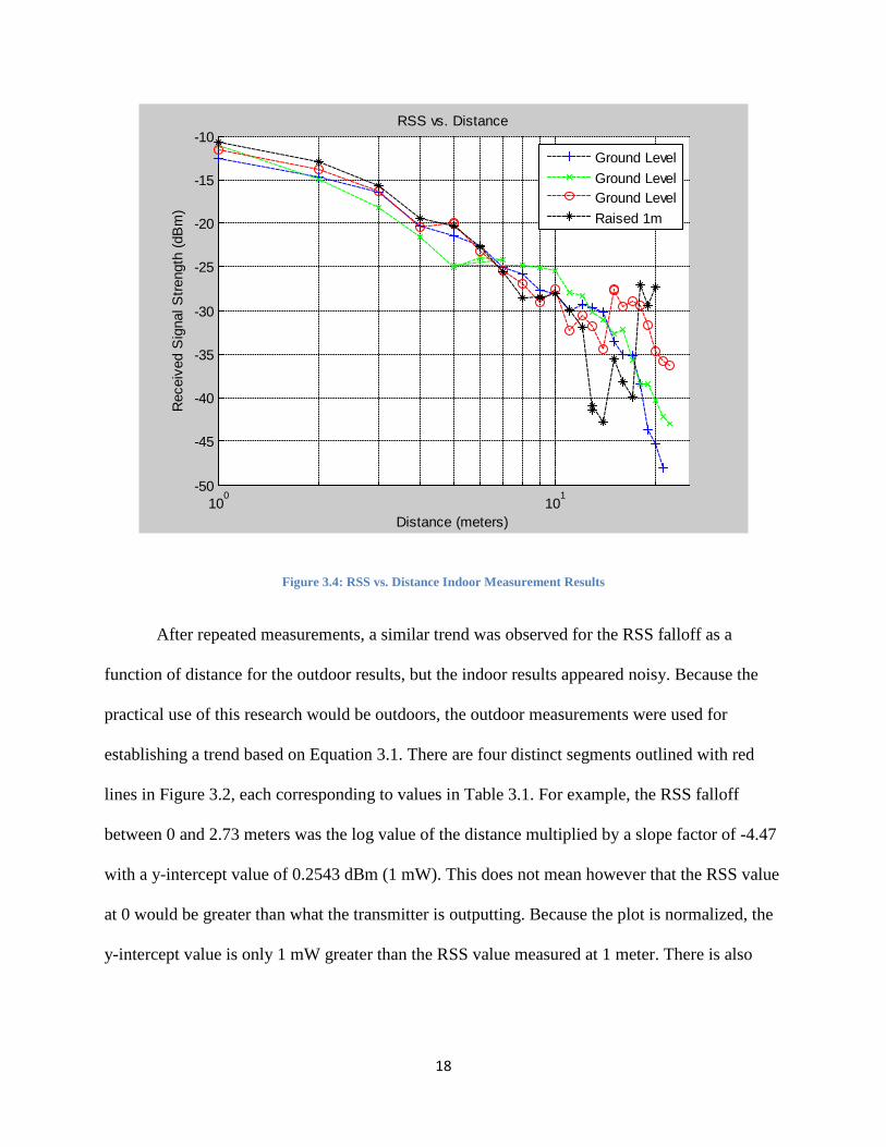
Figure 3.4: RSS vs. Distance Indoor Measurement Results

After repeated measurements, a similar trend was observed for the RSS falloff as a

function of distance for the outdoor results, but the indoor results appeared noisy. Because the

practical use of this research would be outdoors, the outdoor measurements were used for

establishing a trend based on Equation 3.1. There are four distinct segments outlined with red

lines in Figure 3.2, each corresponding to values in Table 3.1. For example, the RSS falloff

between 0 and 2.73 meters was the log value of the distance multiplied by a slope factor of -4.47

with a y-intercept value of 0.2543 dBm (1 mW). This does not mean however that the RSS value

at 0 would be greater than what the transmitter is outputting. Because the plot is normalized, the

y-intercept value is only 1 mW greater than the RSS value measured at 1 meter. There is also

100

101

-50

-45

-40

-35

-30

-25

-20

-15

-10

Distance (meters)

Rec

eive

d S

igna

l Stre

ngth

(dB

m)

RSS vs. Distance

Ground LevelGround LevelGround LevelRaised 1m

19

uncertainty based on possible interference, but this is just an approximation. The rest of the

piecewise fit line can be completed by inserting the values from Table 3.1 into Equation 3.1.

𝑅𝑆𝑆𝑑𝐵𝑚 = 𝑆𝑖 ∗ log10(𝑑𝑖𝑠𝑡𝑎𝑛𝑐𝑒) + 𝑏𝑖 ( 3.1 )

Equation 3.1 includes the received signal strength in decibels (RSSdBm), the slope of each portion

of the piecewise function (Si), and the y-intercept associated with each portion of the piecewise

function (bi).

Table 3.1: RSS vs. Distance Piecewise Linear Fit Values for Outdoor Experimentation of Figure 3.2

i Range Slope (Si) Y-intercept (bi) 1 0m < d ≤ 2.73m -4.47 0.2543 2 2.73m < d ≤ 8.74m -24.14 8.82 3 8.74m < d ≤ 17.61m -61.78 44.27 4 d ≥ 17.61m -186.84 200.1

With the indoor range measurements, the possible discrepancy is a result from the large spinning

metal tower within the range. Although the results were similar, they are unreliable for

determining a piecewise fit to compare with the outdoor results. For this reason, the outdoor

results were used as the base values. The piecewise linear fit for this solution does not agree with

the theory presented in Section 3.4: RSS vs. Distance Test but was used because of the

repeatability of the measurements.

3.5 Antenna Test Pattern

The second test that was conducted in each testing environment regarded determining the

antenna pattern. The importance of this test came from visualizing the front and back lobes of the

log-periodic antenna as well as the nulls. Because received signal strength is the only other piece

20

of information used in the calculation of a location for a specified signal, this test allowed the

equipment to measure the angle from which the signal originated, rather than incorporate more

test equipment with the sensor system to provide this information. For testing the research

hypothesis, a low accuracy antenna was used. Although the log-periodic antenna has a “front”

and “back” side, it is not capable of viewing a signal to within a degree and can be considered a

broadband antenna, meeting the hypothesized specification.

Because this type of test was conducted differently between the indoor and outdoor

testing environments, the indoor range version of this is detailed in Section 3.6: Indoor Range

Testing. The equipment for the outdoor antenna pattern measurements included the emitter and

receiver testbeds, a 30 meter measuring tape, a router, a base station (i.e., a laptop computer),

and an orienteering compass. The tape measure was placed across the ground to the extent of 5

meters. The emitter testbed was then placed with the monopole antenna located above the 0

meter mark of the tape measure. These two items remained fixed after setup. For testing, the

receiver testbed was placed above the tape measure with the log-periodic antenna located exactly

above the 5 meter mark. The laptop received data from the receiver testbed and then the testbed

was rotated approximately 10° to 20°, dependent on each individual test as many tests were

conducted. The orienteering compass was placed on the receiver testbed with the purpose of

allowing the person moving the testbed to visualize how far it had been rotated each time. The

compass was also initially used to verify that the digital compass mounted on the receiver testbed

was reliable. Because the data presented by the orienteering compass and with a grid on the

ground consistently did not match the digital compass, it was decided that the digital compass

was not reliable for obtaining heading angles. The outdoor testing of the antenna pattern had a

similar setup to that shown in Figure 3.1. Instead of having the receiver testbed stationed at

21

variable distances from the transmitter, however, the receiver testbed was placed 5 meters from

the emitter testbed and measurements were obtained while the testbed was rotated 360°. After

each test, the data collected could then be analyzed with MATLAB scripts compiled for this

research. The normalized results from the outdoor antenna pattern measurement for 12 April

2013 are shown in Figure 3.5.

Figure 3.5: Receiver Antenna Pattern, Outdoor Measurement Results

After observing the results of Figure 3.5, two distinct “lobes” were noticed. The front

lobe or main lobe was noticed between the 300° mark and the 90° mark. The half-power

bandwidth of the lobe ranged from 285° and 60° for a total bandwidth of 135°. For the half-

22

power bandwidth calculation, the bandwidth is bound by the 3 dBm drop from the peak signal.

The second lobe present was the back lobe, which was almost as expected. Because of the

geometry of the log-periodic antenna, it was possible to measure small amounts of a signal

through the back of the antenna which resulted in the back lobe. One concern with this

measurement was that the back lobe measured about 45% (nearly half) of the amount of signal

that the main lobe was capable of measuring according to Equation 2.1. Because log-periodic

antennas are generally direction sensitive, the back lobe should only capture a small percentage

of the signal (approximately 10 to 15%) compared with the front lobe; thus, the back lobe of

Figure 3.5 measured a much higher signal than expected for the back lobe measurement.

3.6 Indoor Range Testing

The antenna pattern measurements were conducted both in an outdoor environment and

within the indoor testing range used for the RSS vs. distance measurements. The indoor range

was equipped with hardware that allowed for more automated and reliable antenna pattern

measurements to be achieved. Rather than using the transmitter testbed using the monopole

antenna, the range was equipped with a directive transmitter that was able to reflect a specified

signal off a scattering plate. The scattered signal was then equally distributed over a quiet zone

located approximately 27 feet above the base of the tower. The top of the tower was located 20

feet above the ground, and a completely reflection-free zone was located in the range of 4 to 10

feet above the tower’s top. Fixed to the tower’s platform was a turntable device which was also

used. Because the purpose of this calibration test was to understand the antenna pattern of the

receiver testbed that would later be tested in case studies, it was important that the receiver

testbed be used for this test. The receiver testbed was placed on the turntable device of the tower

23

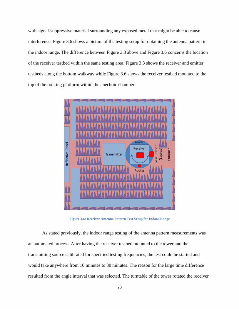
with signal-suppressive material surrounding any exposed metal that might be able to cause

interference. Figure 3.6 shows a picture of the testing setup for obtaining the antenna pattern in

the indoor range. The difference between Figure 3.3 above and Figure 3.6 concerns the location

of the receiver testbed within the same testing area. Figure 3.3 shows the receiver and emitter

testbeds along the bottom walkway while Figure 3.6 shows the receiver testbed mounted to the

top of the rotating platform within the anechoic chamber.

Figure 3.6: Receiver Antenna Pattern Test Setup for Indoor Range

As stated previously, the indoor range testing of the antenna pattern measurements was

an automated process. After having the receiver testbed mounted to the tower and the

transmitting source calibrated for specified testing frequencies, the test could be started and

would take anywhere from 10 minutes to 30 minutes. The reason for the large time difference

resulted from the angle interval that was selected. The turntable of the tower rotated the receiver

24

testbed exactly 360° throughout the entirety of the measurement process. The transmitting source

was continuously sending a signal. The program used for the indoor range testing equipment was

able to read the measured signal of the log-periodic antenna at any time and this was dictated by

the angle interval selected.

Because the testing was being conducted within an ideal zone, it was desired that a

complete data set was taken for multiple frequencies (900 MHz to 1 GHz and 2.3 GHz to 2.5

GHz) which can be tested as the points of interest are located within the ISM band. There was no

noticeable difference between points located 5° apart from the first antenna pattern

measurements of the indoor range using 1° testing intervals and it was then decided that 5°

intervals could be tested, reducing the testing time significantly. The tests for each frequency

were conducted at multiple times to ensure repeatability and included testing the elevation and

azimuth planes of the log-periodic antenna.

The automated test resulted in antenna patterns being obtained for roughly 100 evenly

spaced frequencies within the testing regions listed above. Because the frequency of interest for

analysis with this research was 925 MHz, the corresponding 925 MHz antenna pattern from the

indoor testing could be compared with the outdoor antenna pattern test results. The comparison

of the indoor results and simulation results is shown in Figure 3.7. The simulation results shown

in blue were a result of an antenna modeling program that used the geometry of the log-periodic

antenna to produce the “ideal” measurement with the antenna.

25

Figure 3.7: Receiver Antenna Pattern, Outdoor Measurement Results & Model Data

There are two antenna patterns within Figure 3.7. The red antenna pattern is from

normalized decibel measurements taken within the indoor range while the log-periodic antenna

was mounted to the top of the tower. The blue antenna pattern, as mentioned before, is the

normalized decibel result of simulation software for antennas called Computer Simulation

Technology (CST) [16]. The data collected to obtain an antenna pattern was the work of one of

the members from the undergraduate team at Rose-Hulman. The CST software incorporates the

geometry of an antenna to produce the simulated antenna pattern at any frequency range.

26

When comparing the two patterns, the first difference to be noticed is the lack of a back

lobe on the indoor range results. This is possibly a byproduct of the mount that was used while

taking measurements for the spinning antenna which was later tested in Section 3.7: Range

Gating. A signal-suppressive material was used to cover the metal mount and therefore the signal

was suppressed when it should have been measured on the back end of the antenna. Another

difference to be noted is the magnitude of the indoor range result compared with the simulation

software. The simulation uses no noise or reflections in its calculation of the antenna pattern

while the indoor range result dealt with a large metal platform to cause a bit of interference in an

indoor range that was not perfect at eliminating all reflections, as mentioned with the lack of a

back lobe before. Also as mentioned before with the outdoor measurement, from the computer

simulation a back lobe of less than 25% of the magnitude should be possible, although most of

the back lobe is closer to 15% of the normalized maximum. Because of the back lobe issue in the

Figure 3.7, a method referred to as range-gating was used to see if another measurement process

could be used to obtain a more realistic model of the log-periodic antenna’s pattern.

The antenna patterns of Figure 3.5 and Figure 3.7 are on separate scales because of the

programs used for their creation. Figure 3.5 was the result of a MATLAB script that allowed the

normalized antenna pattern to be created while Figure 3.7 was plotted in Microsoft Excel and

resulted in a normalized plot on the decibel scale. For conversion of these units, Section 3.7:

Range Gating discusses how to compare the two plots.

3.7 Range Gating

The procedure referred to as range-gating was introduced as a way to remove as much

reflection interference effects as possible with the indoor range measurements of the antenna

27

pattern due to the tower and other related equipment in the range. For this process, there are six

steps to complete [17]. First, a suitable bandwidth needed to be selected in order to be able to

determine which of the paths the desired path was, and which paths introduced multi-path

reflection. The bandwidth selected for this testing ranged from 900 MHz to 2 GHz as shown in

Figure 3.8, with emphasis on the range-gating measurements to include 911 MHz to 938.5 MHz,

approximately 14 MHz on each end of the 925 MHz that was being measured throughout this

research. The next step required the frequency response of each rotation angle be measured. The

rotating platform on the tower was used for this step. The Fourier transform of each frequency

response obtained the “range profile” at each rotation angle for the third step. The fourth step

used a window filter around the center frequency at each frequency response to eliminate any

multi-path reflection. Using the inverse Fourier transform, the power response was obtained at

each rotation angle. Finally, as shown in Figure 3.9, the plot of the gain vs. the rotation angle

was obtained. The plots for Figure 3.8 and Figure 3.9 are the result of a MATLAB script

developed by Tim Tanigawa at the Air Force Research Laboratory.

The setup for this testing procedure was similar to that of the antenna pattern

measurements with the exception that the antenna was mounted alone to the top of the rotating

platform on the tower. After obtaining one set of measurements, the antenna was shifted roughly

16 cm in order to create a half-wave offset.

28

Figure 3.8: Calibrated Gain vs. Frequency for Range Gating

Because the testing frequency was 925 MHz, it was useful that the calibrated gain vs.

frequency be determined to eliminate any multi-path effects. Because of the number of

measurements taken between 911 MHz and 938.5 MHz, the closest frequency to 925 MHz was

924.75 MHz. The plot for calibrated gain vs. rotation angle is shown in Figure 3.9.

800 1000 1200 1400 1600 1800 20001

1.5

2

2.5

3

3.5

4

4.5

5

5.5Calibrated Gain Versus Frequency

Frequency (MHz)

Gai

n (d

Bm

)

29

Figure 3.9: Calibrated Gain vs. Rotation Angle for Range Gating

The peak of the plot in Figure 3.9 is just below 3 dBm. Because power is halved at 3

dBm below the peak, the front lobe’s bandwidth spans from approximately -50° to 100°, with a

small amount of spurious signal around 90°. Outside of this range, the measurable gain becomes

much smaller. There is, between 160° and 200°, a back lobe present. The difference between the

maximum magnitude of the front lobe and the maximum magnitude of the back lobe shows that

the back lobe only measures about 20% of the magnitude of the front lobe. This is based on the

idea that for every 3 dBm drop, the power halves. This is calculated using the equation 10-3/10 =

0.50. The back to front lobe ratio is calculated from 10-7/10 = 0.1995. This 20% maximum

30

magnitude for the back lobe matches well with the computer simulation’s results of 15% to 25%

as shown in Figure 3.7.

3.8 Summary

With the use of these calibration tests, a model of the log-periodic antenna could be

created to include the RSS vs. distance falloff and the antenna pattern for the log-periodic

antenna. The RSS vs. distance calibration tests defined the signal falloff as the receiver testbed

was either closer or farther from the signal origin. The antenna pattern calibration test was used

to create a model for how the antenna measured a signal across an entire 360° area. The

normalized magnitude specifies how strong of a signal appears when measured equally from all

sides. The range gating procedure helped to eliminate reflections and interference effects of the

antenna pattern result from the indoor range. The indoor range result could then be compared

with the computer simulation to verify that the two results matched. The RSS vs. distance model

and the antenna pattern model are used in the simulation model when testing the feasibility of the

system. The two models are incorporated into MATLAB code to test on a scaled grid, explained

more in Chapter 4: Objective 2 - Feasibility.

31

4. OBJECTIVE 2 – FEASIBILITY


In this chapter, the hypothesis is reviewed and the results and analysis of the case study

testing to prove system feasibility are provided.

4.2 Outdoor Range Testing/Test Scenarios

The objective of this research was to test the hypothesis that a sensor network can employ

low accuracy, low cost, coarse direction finding sensors in an effort to locate some signal of

interest without compromising precision or accuracy. The first main objective was to model the

receiving antenna through calibration tests. The second objective was to understand how

practical the sensor system is through test scenarios. To do this, a testing grid of 50 meters by 50

meters was created across the ground, and then multiple “flight paths” were marked on the grid

to represent measurement locations to match simulation measurement points in MATLAB.

Figure 4.1 shows how the testing grid was designed within the outdoor testing range with the

flight path lines and emitter locations to be used for testing. Within the figure are both red dots

along green lines to represent the 5 meter marks and the X- and Y-axes created to have a grid to

match the simulation testing. The X-axis is along the right side of the figure and the Y-axis is on

the top side. The green lines intersect at (50, 0) rather than the typical (0, 0) intersection point.

The red and yellow dashed lines signify the testing paths begin at the same point (20, 20) and

extend in different directions. The red line was used for test scenario #1 and the yellow line for

test scenario #2. Along each of these paths, measurements were to be taken every 2.5 meters to

match the 250 meters per step that the simulation was used. The green dots in the figure

32

represent each of the emitter locations that were used for testing, with each dot corresponding to

a different flight path. Everything with the grid was scaled by a factor of 1/100 to the simulation

testing to compare nearly identical testing areas.

Figure 4.1: Test Scenario Layout for Outdoor Experimentation

4.3 Goals and Hypotheses

The MATLAB scripts used to localize emitters in previous research was now retrofitted

to incorporate a CS solver which could quickly solve the problem of determining an unknown

number of signal locations. For this reason, the measurements obtained through the test scenarios

would be added into the MATLAB simulation for calculations. The goal of these test scenarios

was to obtain both precise measurement locations and RSS measurements. At each measurement

33

point of the receiver testbed and the stationary emitter location, the X and Y coordinates were

noted for comparison to the MATLAB coordinates. The RSS values could also be compared

with the simulation’s measurements. More so, the RSS values were necessary to actually add to

the MATLAB simulation. Rather than overwriting MATLAB’s calculations for the RSS values

at each point, the RSS values from the test scenarios were input into the code so the CS solver

could, to some degree, attempt to localize an emitter solution based on the test scenario values.

4.4 Localization Techniques

4.4.1 How Others Do It

Section 3.3: Definition of Terms introduced multiple techniques that are used in

geolocation and localization. Though this section only covers a handful of techniques, there

are many other techniques that are capable of being used to perform similar activities. Time

difference of arrival (TDOA) and angle of arrival (AOA) were briefly discussed previously.

Two other similar techniques are frequency difference of arrival (FDOA) and time of arrival

(TOA). FDOA is similar to TDOA in that the technique measures a difference in a

transmitted signal. The difference is that FDOA measures the Doppler shift, requiring more

data to be sent between the measurement points. TOA is a technique that measures an

absolute time difference at a single measurement point rather than multiple points to send and

receive a signal. This technique is similar to a speed detector which sends a signal to a

potential speeder and then receives the signal, before sending another to measure the speed of

the object. Because this research does not focus on other techniques, less detail is required at

this time. The reasons for explaining the different techniques are only to exemplify how

complicated they can be to measure the origin of a signal when even multiple sensors and

34

multiples schemes are used. For this research, though, it is hypothesized that through the use

of compressed sensing only sensors that are equipped with low cost, low directivity

equipment are capable of working together to localize a signal of interest with similar

precision and accuracy as when using the techniques and algorithms mentioned above.

4.4.2 Compressed Sensing

This research introduces compressed sensing as a means to solve a highly complex

problem involving coarse measurements with speed, precision, and accuracy as compared

with similar approaches mentioned in Section 4.4.1: How Others Do It. The keys to being

able to use this process include not adding additional latency time to calculate localized

solutions and also doing so without losing the precision and accuracy that might be obtained

through other localization techniques. As explained in Section 2.5: Compressed Sensing, CS

is capable of taking a large matrix of mostly sparse data and equating a solution. In the case

of this research, the matrix is comprised of each point of the grid used for testing. This means

with the scenario testing the matrix has 50 rows and 50 columns. In each of the scenarios

tested, there were at most two emitters present. Within the matrix there could only be two

points where the value was much larger than the rest of the data. Because CS works with

linear types of data, the noise floor measurements represent the null data elements of the

matrix. This helps to establish a mostly sparse matrix or grid.

For the computer simulations and for comparing the test scenarios to them, a CS

solver was incorporated with the MATLAB programs. This software could handle large

amounts of data and solve the highly complex problems that would be too time-consuming to

do any other way.

35

4.5 Test Scenario #1

For test scenario #1, a path was randomly created using MATLAB with an emitter

located at the very center of the testing area as shown in Figure 4.2a, with the testing path

represented with a red dashed line and the actual emitter location represented with a star. Using

the MATLAB programs, the path was shown to be able to localize a solution for the emitter

location. Therefore, it should be possible for the receiver testbed to use CS to accurately localize

the emitter’s position as well. Figure 4.2b shows the receiver testbed indicated by the white

arrow. Also useful with this diagram is the X used to indicate the localized position of the emitter

and the pink pixel, both located in the same position. The CS solver is able to compute the

probability of the emitter being in a given position within the testing grid and assigns each value

of the matrix a probability percentage of containing the emitter. Because the MATLAB

simulation localizes the emitter to a small region, as denoted by the single pink pixel, the

solution is highly probable to lie within this area compared with anywhere else in the grid.

Before enough data points are collected, however, this location will not be exact, as is shown in

Figure 4.2a with the X on the side of the grid and not within the actual location of the emitter.

Figure 4.2: (a) Emitter Location Unknown (left) and (b) Localized Emitter Location (right) for Test Scenario #1

36

The bottom of Figure 4.2b includes some useful information. With this case, the CS

algorithm could determine the answer to the simulation in five time steps. This means that for

this example, only five measurements are necessary from a single receiver to correctly localize

the emitter’s position. This is not a general result, but shows how simple the process can be.

With this example, the accuracy of the localization equates to 70.7 meters within a 5000 meter

by 5000 meter testing grid. The value is not zero because the emitter location is actually located

at the center of a pixel while the CS solver is only able to localize a solution to the corners of a

pixel. 70.7 meters on this testing area is the distance from the center of a pixel to any of its

corners. Because the problem can easily be rescaled, these numbers are just arbitrary and are not

exact for each case.

4.6 Test Scenario #1 Results

From the solution presented by the MATLAB simulation, it could be expected that it is

possible to localize an emitter to a precise area within no fewer than 5 time steps as the solution

has completely clean, reflection-free measurements. Because the data collected at the outdoor

range was not perfect, in part from using low accuracy, low cost, coarse direction finding

sensors, it was expected that more than 5 data points would need to be collected. The receiver

testbed was moved along the designed path while measurements were obtained every 2.5 meters

to mimic 250 meters per second of velocity of the simulation receiver with measurements once

per second. There were a total of 30 measurements taken at each point, with 30 data points to

measure. After post-processing the data, the first 16 data points contained “reliable” data with the

rest being unused.

37

Figure 4.3 shows the MATLAB simulation window that was the result of the RSS

measurements being plugged into the program. From the response that the program gives, there

are clearly errors with both the program and the measurement data. Also, when there is an error

from the program, the axes do not generate and the entire test space has a 100% chance of

including the emitter without an indicator from the software to denote the estimated location.

The program and the CS solver are capable of working together to solve this same problem and

the data points that the program measures can be read out for comparison. As a way to compare

the simulated and measured data, Table 4.1 lists each at the first 10 data points of the testing path

for scenario #1.

Figure 4.3: Test Scenario #1 Path with "Error Reported"

after iteration 10

Nor

mal

ized

Em

itted

Pow

er

0

0.1

0.2

0.3

0.4

0.5

0.6

0.7

0.8

0.9

1

38

Table 4.1: Simulated vs. Measured RSS Values for Test Scenario #1

Time step

Simulated RSS (dBm)

Measured RSS (dBm)

1 -566.7850 -36.6879 2 -66.9486 -26.2029 3 -66.1206 -18.4566 4 -56.3472 -15.2490 5 -63.9925 -13.8612 6 -78.0844 -21.4015 7 -73.8473 -33.7489 8 -96.3121 -42.3575 9 -551.1461 -42.1785 10 -629.0995 -47.4084

There are two things to understand from Table 4.1. The first point is that there is a slight

correlation between the simulated and measured RSS. As the measured RSS values increase, the

simulated RSS values increase as well. When the measured RSS values decrease, the simulated

RSS values decrease. The closest point to the emitter testbed on the testing path occurs at time

step 5, exactly how the measured RSS column depicts. The second point to notice is how much

the two columns differ. The measured RSS data do not vary much relative to the magnitude of 20

differences with the simulated RSS data. No explanation for this has been accurately

hypothesized. The simulation is capable of using these numbers to solve the localization of the

emitter, but the true values can either produce inaccurate localizations or an “error” according to

the CS solver. These two simultaneous occurrences do not seem to correlate with one another. If

the receiver is truly getting closer to the emitter and detects a stronger signal and the signal can

also decrease when the antenna does not aim in the direction of the emitter, it seems likely that

the CS solver would be able to detect an offset of some sort to solve the problem free of errors.

39

4.7 Test Scenario #2

Similar to test scenario #1, the second test scenario used a randomly created path that

demonstrated promise in regards to accurately locating an emitter’s position. There were two

very similar setups tested in simulation for this case. One case used a single emitter located at

point (3000, 2000) while the other, as shown in Figure 4.4a, used a second emitter positioned at

point (1500, 3500). Due to Wi-Fi connectivity constraints within the outdoor testing area to

connect to each of the three devices needed for testing, the second emitter was omitted from test

scenario #2 measurements. Only the emitter at (3000, 2000) remained. The MATLAB

simulations showed that there is no change in emitter localization when only one emitter is used

versus two. The CS solver is still able to handle the change and each emitter is localized in the

same number of time steps, regardless of the number of other emitters which the receiver might

be able to measure while simulated. For this reason, there was no concern moving forward with

only the one emitter present in the testing area.

The bottom section of Figure 4.4b shows that in order to accurately locate both of the

emitters in the simulation, ten time steps would be necessary. Only four time steps were

necessary to locate the emitter at (1500, 3500) but it wasn’t until 10 time steps were completed

that the second emitter was located. When the first emitter is not present, as was the case for the

outdoor testing, ten time steps were still necessary according to the simulation to localize on the

emitter. When these emitter’s were created as text files for the simulation to use, they were

actually generated with their centers on the corners of pixels. For this reason it is possible that

the accuracy is equal to 0 meters offset from the actual locations. Again, the X that represents the

40

localization is within the single pink pixel which represents solutions that are very precise

compared with the overall grid space.

Figure 4.4: (a) Emitter Locations Unknown (left) and (b) Localized Emitter Locations (right) for Test Scenario #2

4.8 Test Scenario #2 Results

For test scenario #2, there were 30 data points to be measured with 30 RSS measurements

obtained at each data point. Due to a mechanical malfunction, only the first 17 data points were

able to be captured for post-processing. Because there were still more than the fewest number of

data points necessary per the simulation, and because of time constraints for the availability of

the testing area, the 17 data points were considered acceptable.

Figure 4.5 shows the similarity between the simulation results for test scenario #1 and

test scenario #2, which also results with “error reported” as the output from MATLAB. The

program is unable to calculate any sort of location for the emitter based on the measured RSS

values going out to 15 data points. Unlike the results of scenario #1, however, the simulation

RSS values do not balloon to such extreme values, as is shown in Table 4.2.

41

Figure 4.5: Test Scenario #2 with "Error Reported"

With the exception of the simulated RSS at time step one, the values of Table 4.2 initially

have similar trends. The CS solver is able to localize an emitter location based on the simulated

results, but not using the measured RSS values. One hypothesis for this case could be that the

simulated RSS values have a considerable change in signal strength over the course of the test

path while the measured signal does not vary as much.

after iteration 14

Nor

mal

ized

Em

itted

Pow

er

0

0.1

0.2

0.3

0.4

0.5

0.6

0.7

0.8

0.9

1

42

Table 4.2: Simulated vs. Measured RSS Values for Test Scenario #2

Time step

Simulated RSS (dBm)

Measured RSS (dBm)

1 -8.438110-5 -13.8095

2 -12.1203 -14.6288 3 -12.1654 -16.1556 4 -15.2055 -18.3453 5 -15.3540 -20.8611 6 -57.8917 -23.7286 7 -109.5424 -25.0367 8 -117.1915 -27.4573 9 -124.0281 -30.9817 10 -127.8085 -34.6878

4.9 Summary

When conducting the experimentation for test scenarios #1 and #2, the test paths that

were modeled had shown no indication of failure. The measurement points were shown to work

well in simulation when using the CS solver and MATLAB hand-in-hand to calculate received

signal strength values and compute a localization of the emitter. The measurement points were

mapped out with precision, being located no more than 10 cm from the point at which MATLAB

used. Multiple measurements were obtained at each test point for analysis. When examining the

data’s trends throughout the measurement paths, a pattern appeared that was seemed hopeful for

determining a location as simply as the program was capable of doing. As the receiver was

directed or placed near to the emitter, RSS readings were strong. When the emitter was not in

view of the receiver, the measurements approached the noise floor as would be expected.

Rather than allowing the simulation to calculate the signal strengths, the code was

replaced to read the measured RSS values. The solver received the RSS data from MATLAB to

compute and map out a solution within the testing grid. The end result, however, was that no

43

solution could be determined. A couple possible reasons for the inability of the simulation

software to compute a reliable localization could have come from the solver itself. The tool used

was free software for academic use but the compatibility with MATLAB might have had

underlying issues. Another, and more likely hypothesis, deals with the RSS falloff function

created. Because everything in MATLAB was without units, the simulation had no way of

knowing if the grid was 5000 meters squared or 50 meters squared. For this reason, it was

assumed that the piecewise function would work linearly between the two testing grids. What

might actually be true is that the grid was based off a particular order of magnitude (i.e., 1,000)

while the piecewise fit was based on ten. This could create a non-linearity with the problem. This

hypothesis was never proved or disproved.

44

5. CONCLUSIONS AND RECOMMENDATIONS


In this chapter, a summary of the research results are provided, the significance of the

results as they pertain to the hypothesis is discussed and recommendations for future work on the

capability of localizing an emitted signal are given.

5.2 Research Conclusions

After reviewing the plot of Figure 3.2 on page 15, the RSS vs. distance test does not

appear to be valid. The reasoning for this judgment is that the plotted data does not appear linear

on the log-log plot as should be expected, with a slope on the plot somewhere between negative

two (in the absence of a ground plane) and negative four (for environments with a perfect ground

plane) as was mentioned in Section 3.4: RSS vs. Distance Test. One hypothesis for this sudden

falloff as a function of distance was the result of the battery losing power as the tests were

conducted. Because every test started at 1 meter of separation between the two testbeds and

moved out to 30 meters throughout the test, time could be a factor for the battery discharging on

the emitter testbed and producing a weaker signal over time. To test this hypothesis, both the

power supplies of the receiver and emitter testbeds were replaced with AC power supplies for

constant power. The result of this alteration would help to demonstrate if battery loss were

responsible for the unexplained patterns being produced with the RSS vs. distance

measurements. The result of this alteration is shown in Figure 5.1. From comparison of multiple

points on the plot, a similar pattern is present. A slow linear drop through the first 15 to 17

meters is present with the sudden falloff coming beyond this point.

45

Figure 5.1: RSS vs. Distance Measurement with AC Power, Log-Periodic Antenna

Because there is no significant difference between when a battery pack is used to power

the testbeds and when AC power is applied, another difference to test concerned the antenna of

the receiver testbed. For the calibration tests and throughout the case scenario testing, the log-

periodic antenna was mounted to the receiver testbed. To test the possibility of this antenna

creating the unexplained effect with the plotted data, an omnidirectional antenna replaced the

log-periodic antenna and the RSS vs. distance test was replicated. Again, a similar sudden drop-

off appears in the received signal strength around the 15 meter point, although not as sudden as

before, as shown in Figure 5.2. The testing of this hypothesis still does not demonstrate where a

problem is occurring for the testing. Because the last two tests have shown that the RSS vs.

distance curve is repeatable, both the power supply and the receiving antenna can be ruled out as

factors for the repeatable behavior. Another alteration to the testing with the omnidirectional

0 0.2 0.4 0.6 0.8 1 1.2 1.4 1.6-100

-80

-60

-40

-20

0

20

Log Distance (m)

Nor

mal

ized

Rec

eive

d Si

gnal

Stre

ngth

(dBm

)Normalized RSS vs. Distance with AC Power, Log-Periodic Antenna

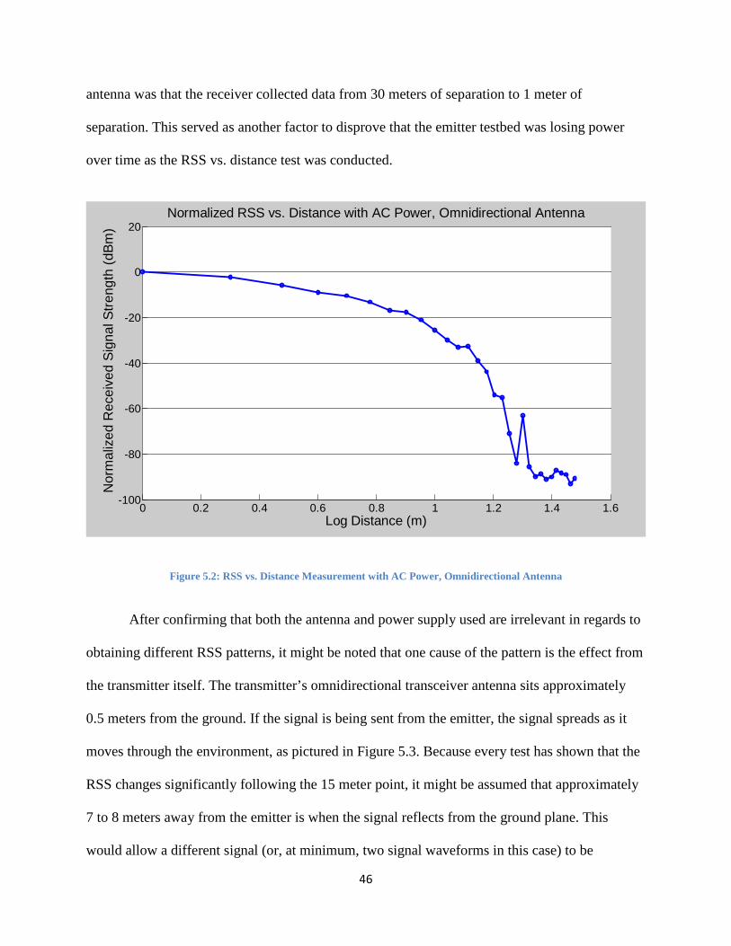
46

antenna was that the receiver collected data from 30 meters of separation to 1 meter of

separation. This served as another factor to disprove that the emitter testbed was losing power

over time as the RSS vs. distance test was conducted.

Figure 5.2: RSS vs. Distance Measurement with AC Power, Omnidirectional Antenna

After confirming that both the antenna and power supply used are irrelevant in regards to

obtaining different RSS patterns, it might be noted that one cause of the pattern is the effect from

the transmitter itself. The transmitter’s omnidirectional transceiver antenna sits approximately

0.5 meters from the ground. If the signal is being sent from the emitter, the signal spreads as it

moves through the environment, as pictured in Figure 5.3. Because every test has shown that the

RSS changes significantly following the 15 meter point, it might be assumed that approximately

7 to 8 meters away from the emitter is when the signal reflects from the ground plane. This

would allow a different signal (or, at minimum, two signal waveforms in this case) to be

0 0.2 0.4 0.6 0.8 1 1.2 1.4 1.6-100

-80

-60

-40

-20

0

20

Log Distance (m)

Nor

mal

ized

Rec

eive

d Si

gnal

Stre

ngth

(dBm

)

Normalized RSS vs. Distance with AC Power, Omnidirectional Antenna

47

measured at the receiving testbed’s antenna, regardless of the antenna used, thus creating a

different appearance to the collected data. Within Figure 5.3, when the signal reflects off the

ground, it gives the appearance to the receiver that multiple emitters might be present.

Figure 5.3: Diagram of Signal Reflections from Ground Plane

Another factor that was tested in an attempt to measure a linear pattern for the RSS falloff

as a function of distance was to change the ground plane of measurement. All of the previous

testing, with the exception of testing completed in the indoor testing range, had been conducted

on grassy surfaces within open fields. The testbeds were moved indoors to a basketball arena to

incorporate the smooth, even surfaces for a ground plane between them. Figure 5.4 shows that

not only are the RSS measurements linear across the distances measured, the measured RSS

appears stronger at greater distances because there is no point of sudden falloff with the data. As

opposed to measuring near the noise floor of approximately -107 dBm with the receiver testbed

on grassy surfaces, the receiver testbed within the arena was only able to measure an RSS

48

reading of approximately -40 dBm at 40 meters of separation from the emitter, a much larger

distance than was possible with the measurements on the grassy surface. Another factor that

could also have had an impact in the RSS measurements in the arena was the reflections from

any and all walls of the arena, which are likely responsible for the jumps in data for the first 10

meters. Because the distance measured reached 50 meters, it would be highly probable that many

transmitted waves had bounced off nearby objects before being measured by the receiver testbed.

The possible multi-path reception for the receiver might also explain why the signal is much

greater over the 50 meter span than was previously recorded for grassy surfaces.

Figure 5.4: RSS vs. Distance Measurement for Arena Testing

As it relates to the testing completed within this research, conducting the calibration tests

to model the log-periodic antenna and the case scenarios within the arena might have had a much

0 0.2 0.4 0.6 0.8 1 1.2 1.4 1.6-100

-80

-60

-40

-20

0

20

Log Distance (m)

Nor

mal

ized

Rec

eive

d Si

gnal

Stre

ngth

(dBm

)

Normalized RSS vs. Distance for Basketball Floor Ground Plane

49

different impact. Whether it would be a positive or negative impact, however, would depend on

the effects that the arena’s environment would have had on the emitted signals.

Another point to take into account is that for the original intended purposes of this

research (for use with UAVs to locate signals for a given reason), the ground plane effects would

not likely be factors to be concerned with. Assuming the UAVs are flying above the emitted

signals, both the ground plane and any effects from interfering nearby objects would not be

likely. This is with the exception of mountains or cliffs while the emitter lies within a valley of

some sort. Although this testing has not confirmed that this procedure would accurately and

precisely localize signals of interest, it may still be possible.

5.3 Research Significance

As mentioned before, although this research has not produced definite proof that this

procedure for localizing a signal works, there is still promise that it is possible. The ground

plane’s effect on the measured signal shows that a linear trend can be obtained but the effects

from any external interference are unknown at this time. This is a subject that might benefit from

any future research regarding the subject matter.

5.4 Future Research Recommendations

Through multiple tests to collect received signal strength data, the resulting data trends

have not appeared linear as would be expected in theory. This trend might be the result of an

insufficient amount of data collected, a ground plane creating inconsistent multipath effects, or

possibly even a gain control being implemented with the software defined radio. These points

50

should be the focus of future testing. It might still be possible that the RSS data can be linear, but

the conditions of this testing were not best suited for this outcome.

The first test to be tested in verifying if a linear data set can be obtained would be to take

the mobile sensor testbeds, without any modifications, and redo the RSS vs. distance test. While

previous testing was conducted from 1 to 30 meters, the updated test should be carried out to

approximately 50 or 60 meters. The reason for this test is that data might be approaching the

noise floor around 30 meters because this is a possible null for the data. If the test shows that the

data returns to a linear trend, with the exception of the null data, and does contain nulls

throughout the collected data, a linear fit could be measured. There are nulls in the data that can

be created by multipath reflections having equal magnitudes having opposite phases. More

discussion on the creation of nulls is discussed later with Figure 5.5 and Figure 5.6. If a linear fit

can be applied to the data set, this antenna model can be replaced and possibly analyzed through

the MATLAB simulation. If a linear trend cannot be measured, or there is no issue involving

nulls in the data, this test would be inconclusive and other tests should be completed.

A second test in trying to find a data set with a linear fit would include adjusting either

the operating frequency or antenna heights of all testbeds in order to determine if the possible

nulls with the data move. Because all other testing has been completed at 925 MHz, I would

personally recommend adjusting the antenna heights of each antenna to include a 2 to 3 meter

height increase. As shown in Figure 5.5, with both the transmitting and receiving antennas

located approximately 1 meter from the ground plane, any data collected beyond approximately

14 meters could result in nulls for the data. As with Figure 5.5, the line-of-sight path for the

transmitted signal might travel 14 meters, but one wave reflected on the ground plane will travel

51

only a small distance farther. This results in two signals possibly being detected at the receiver

with nearly equal magnitudes. Because the reflected wave comes from the ground plane, it can

also include a phase offset of 180°. When the two signals are then added up, the resulting signal

strength is much smaller than either of the two individual waves.

Figure 5.5: Ground Bounce Null Calculation

By adjusting the antenna heights, it would be expected that this eventual falloff, if data were only

taken for 1 to 30 meters again for the RSS vs. distance test, would come at a larger distance. This

falloff is possibly the downward trend of the nulls being created in the data. If the trend of signal

falloff occurring at larger distances is observed, then any higher possible antenna heights should

be used to redo the testing. Also, because the reflection coefficients for the ground planes and the

phase offsets are also related to the transmitting signal frequency, altering the frequency should

have a similar effect on the RSS data. The lower frequencies should pull the signal falloff closer

to 1 meter and higher frequencies should push the signal falloff away from 1 meter as with the

increase of antenna height. The signal falloff can be part of a larger trend in the data. The

observance of a falloff in the signal might be the creation of a null and the data would be

expected to increase again after the null point. Figure 5.6 shows an example of nulls in a data set

52

which includes the 1/distance2 trend out to the last null, then a 1/distance4 trend observed beyond

this point. This is the origin of the theory that was explained in Section 3.4: RSS vs. Distance

Test. It might be possible that the data collected in previous testing is just a small sample of the

larger picture of Figure 5.6 and the falloff pattern is the result of the first null of the data.

Figure 5.6: Ground Bounce Propagation

If the nulls are observed with the data, the trend for the data without using the null data points

should be used in creating a new model for the antenna.

The next test in determining if a linear trend can be observed with the RSS data would be

to conduct the RSS vs. distance test on a different ground plane. Because testing on the

basketball arena surface showed what might be a possible linear trend in the data, this test should

be further examined with more data points collected out to 50 or 60 meters. From the limited

amount of data already collected, a linear trend to the limit of the testing would be expected in

order to create a new model for the antenna to use with MATLAB. One possible predicament

53

with this test might be the multipath reflections caused by the surroundings, as finding a large

enough open space with a similar ground plane could be difficult. Another predicament with this

test might be that a ground plane that is less lossy, as compared with the grass field, could result

in more nulls being created in the data. As well as measuring more nulls in the data, the data

could result with all the nulls being properly measured. These effects should be considered when

analyzing the resulting data from this test.

The fourth test to be considered to understand why the previous RSS data was not linear,

would be with determining if the SDR from Ettus Research includes an automatic gain control

for higher power signals. The data before and after approximately 8 meters appears to have

different trends. It might be possible that the data before 8 meters was measured to be above a

certain threshold and the SDR automatically suppressed it so the observed signal from the base

station was much smaller than truly measured by the testbed. In order to verify if this is or is not

occurring, the emitter testbed’s output power should be decreased by a factor of two for example.

If the emitter is outputting half of the power that was used with the previous RSS vs. distance

tests and the SDR is having a suppression effect on the data, the newly acquired data should be

less of a significant falloff and more linear overall. The factor to decrease by may have to be

adjusted in order to get all data points to be free of suppression by the SDR. If there is no

automatic gain control within the SDR, measuring data at half of the original transmitted power

should result in a similar falloff in the data as the previous testing. If a linear trend is observed,

the new model of the antenna should be implemented with the MATLAB simulation.

After creating a new model for the antenna which does not include a linear trend to the

RSS data, I believe the next step is to determine if the test scenarios do result in correct

54

localizations for the emitters present. Then, similar testbeds that are designed on model airplanes

or even simple UAVs should be used for testing. Something that is capable of carrying a light

payload (5-8 pounds) could add the wireless components used in this research to collect actual

data in either an open field or a large arena. The testbeds could move about without interference

effects in an attempt to localize the emitted signals in real time, or even with post-processing. As

the work progresses, these capabilities could eventually be implemented with actual UAVs used

with the military or industrial companies whose work is relevant to this research.

5.5 Summary

Regardless of the failure to demonstrate that the procedure hypothesized could work to

accurately localize a given signal of interest, there are still possibilities of proving or disproving

that this process could be successful. There are still opportunities to alter parts of the testing

process in an attempt to obtain improved results as stated in the previous section. The improved

results could be paired with similar test scenarios and it might still be possible to show that a

signal can be localized with both precision and accuracy using the low cost sensors and

employing broadband, low directivity antennas.

55

LIST OF REFERENCES

[1] Stoep, J. V. “Design and Implementation of Reliable Localization Algorithms Using Received Signal Strength.” MS Thesis, University of Washington, Seattle, WA, 2009. Web. 3 Feb. 2014. <http://www.ee.washington.edu/research/nsl/Imote/vanderstoep_thesis.pdf>

[2] MATLAB. Natick, MA: The Mathworks, Inc., 2014. Computer software.

[3] Sensor Platform Configuration. “Low level Diagram.” ECE462 Team10 Final Report. 2014. Paper. 31 Mar. 2013.

[4] Ettus Research. Ettus Research, 2004. Web. 3 Feb. 2014. <http://ettus.com>

[5] Waghray, N. “Electronic Warfare: The Next Step in National Security.” India Conference (INDICON), (2011): 1-18. Web. 3 Feb. 2014. <http://ieeexplore.ieee.org/xpls/abs_all.jsp?arnumber=6139348>

[6] Spezio, A. E. “Electronic Warfare Systems.” Microwave Theory and Techniques, 50.3 (2002): 633-644. Web. 3 Feb. 2014. <http://ieeexplore.ieee.org/xpls/icp.jsp?arnumber=989948>

[7] Candes, E. J., and Wakin, M. B. “An Introduction to Compressive Sampling.” Signal Processing Magazine, 25.2 (2008): 21-30. Web. 3 Feb. 2014. <http://ieeexplore.ieee.org/stamp/stamp.jsp?tp=&arnumber=4472240>

[8] Bryan, K. and Leise, T. “Making Do with Less: An Introduction to Compressed Sensing.” SIAM Review, 55.3 (2013): 547-566. Web. 3 Feb. 2014. <http://epubs.siam.org/doi/pdf/10.1137/110837681>

[9] Schneider, D. “New Camera Chip Captures Only What It Needs.” IEEE Spectrum, (2013): 13-14. Web. 4 Apr. 2014. <http://ieeexplore.ieee.org/stamp/stamp.jsp?tp=&arnumber=6471041>

[10] Gang, H. et al. “Lensless Imaging by Compressive Sensing.” Image Processing (ICIP), (2013): 2101-2105. Web. 4 Apr. 2014. <http://ieeexplore.ieee.org/stamp/stamp.jsp?tp=&arnumber=6738433>

[11] Zhang, X. and Lam, E. Y. “Sectional Image Reconstruction in Optical Scanning Holography Using Compressed Sensing.” Image Processing (ICIP), (2010): 3349-3352. Web. 4 Apr. 2014. <http://ieeexplore.ieee.org/stamp/stamp.jsp?tp=&arnumber=5652768>

[12] Zhu, Z. et al. “Compressed Sensing MRI by Two-Dimensional Wavelet Filter Banks.” Multidimensional (nD) Systems (nDs), (2011): 1-6. Web. 4 Apr. 2014. <http://ieeexplore.ieee.org/stamp/stamp.jsp?tp=&arnumber=6076845>

56

[13] Lin, Z. et al. “Infrared Face Recognition Based on Compressive Sensing and PCA.” Computer Science and Automation Engineering (CSAE), (2011): 51-54. Web. 4 Apr. 2014. <http://ieeexplore.ieee.org/stamp/stamp.jsp?tp=&arnumber=5952421>

[14] Roxin, A., et al. “Survey of Wireless Geolocation Techniques.” Globecom Workshops, (2007): 1-30. Web. 3 Feb. 2014. <http://ieeexplore.ieee.org/stamp/stamp.jsp?tp=&arnumber=4437809>

[15] Black, B. A. et al. Introduction to Wireless Systems. Upper Saddle River, NJ: Prentice Hall, 2008. Print.

[16] CST. Framingham, MA: CST of America, Inc., 2014. Computer software.

[17] Li, H. J. et al. “Antenna Measurements in the Presence of Multipath Waves.” Progress in Electromagnetics Research, (2001): 157-178. Web. 3 Feb. 2014. <www.jpier.org/PIER/pier30/08.0002091.Li.LL.pdf>

57

APPENDIX A

Appendix A shows the data tables for the linear piecewise fit established from initial RSS

vs. distance testing and for comparison between simulated and measured RSS data values from

the test scenarios.

Table A.1: RSS vs. Distance Piecewise Linear Fit Values for Outdoor Experimentation of Figure 3.2

i Range Slope (Si) Y-intercept (bi) 1 0m < d ≤ 2.73m -4.47 0.2543 2 2.73m < d ≤ 8.74m -24.14 8.82 3 8.74m < d ≤ 17.61m -61.78 44.27 4 d ≥ 17.61m -186.84 200.1

Table A.2: Simulated vs. Measured RSS Values for Test Scenario #1

Time step

Simulated RSS (dBm)

Measured RSS (dBm)

1 -566.7850 -36.6879 2 -66.9486 -26.2029 3 -66.1206 -18.4566 4 -56.3472 -15.2490 5 -63.9925 -13.8612 6 -78.0844 -21.4015 7 -73.8473 -33.7489 8 -96.3121 -42.3575 9 -551.1461 -42.1785 10 -629.0995 -47.4084

58

Table A.3: Simulated vs. Measured RSS Values for Test Scenario #2

Time step

Simulated RSS (dBm)

Measured RSS (dBm)

1 -8.438110-5 -13.8095

2 -12.1203 -14.6288 3 -12.1654 -16.1556 4 -15.2055 -18.3453 5 -15.3540 -20.8611 6 -57.8917 -23.7286 7 -109.5424 -25.0367 8 -117.1915 -27.4573 9 -124.0281 -30.9817 10 -127.8085 -34.6878

emitter localization and compressed sensing: a low cost

Documents