emittance measurement algorithm and application to himm

EMITTANCE MEASUREMENT ALGORITHM AND APPLICATION TO HIMM CYCLOTRON*

Yong Chun Feng†,1, Rui Shi Mao1, Xiao Juan Wei Institute of Modern Physics, Chinese Academy of Sciences, 730000 Lanzhou, China

1also at Lanzhou Kejintaiji Corporation, LTD, 730000 Lanzhou, China

Abstract HIMM, a Heavy Ion Medical Machine, developed by In-

stitute of Modern Physics, has been in operation since April 2020. The beam emittance of the cyclotron exit is measured with the most often used techniques, i.e. slit-grid, Q-scan and 3-grid at a dedicated beam line which is not the actual HIMM optical line. The high speed data acquisition archi-tecture is based on FPGA, and motion control system is constructed based on the NI module.

The data post processing and emittance calculation is based on Python code with self-developed algorithm, in-cluding Levenberg–Marquardt optimization algorithm, thick lens model, dispersion effect correction, error bar fit, mismatch check, image denoise and “Zero-thresholding” calculation. The algorithm description and simulation are discussed in detail. The application of the algorithm to HIMM cyclotron is presented in this paper as well.

INTRODUCTION The heavy ion medical machine (HIMM) is developed

by the Institute of Modern Physics (IMP), which consists of two electron cyclotron resonance (ECR) ion sources, a cyclotron, a synchrotron ring and five nozzles [1]. The syn-chrotron has a compact structure with a circumference of 56.2 m. The layout of the HIMM complex is shown in Fig. 1. Up to now, the slow-extraction efficiency of HIMM has reached nearly 90% for all energies from 120 to 400 MeV/u. The spill duty factor has exceeded 90% at a sample rate of 10 kHz with the feedback-based slow-ex-traction technique applied [2, 3].

Figure 1: Layout of the HIMM complex.

Cyclotron, as the injector, plays a critical role in HIMM complex, which delivers the high quality beam to the ring through the MEBT (median energy beam transport line). The emittance and TWISS parameters measurement at the

exit of the cyclotron are essential. Before integrating the cyclotron into HIMM, a dedicated beam line is constructed temporarily at the laboratory, and the measurement of emit-tance is performed along it.

The emittance and TWISS parameters at the exit of the cyclotron are measured using three most commonly used methods, slit–grid [4-6], Q-scan [7-9] and 3-grid [8-10]. A cross-check is of capability to validate this measurement.

In this paper, optimizition algorithm for Q-scan and 3-grid is introduced, in which dispersion correction and thick lens model fit are of the most importance in improving the reconstruction accuracy of the emittance. In addition, slit-grid algorithm, especially denoising in reconstrucing the beam phase space is interpreted also. Both the optimizition algorithm and denoising process can result in a positive im-provement for emittance calculation from the view point of simulation and analytic derivation. Finally, the measure-ment results of the cyclotron are presented.

ALGORITHM DESCRIPTION AND SIMULATION

Optimizition Algorithm for Q-scan and 3-grid In the approximation of linear, beam transport along a

lattice can be expressed in the form of matrix, which indicate how the transfer elements impose a function to the beam. From the view of matrix point, a transfer matrix can be formulated as

𝑀 𝑎 𝑏𝑐 𝑑

(1)

without the loss of generality. The matrix must be symplec-tic, which is a remarkable property of a Hamiltonian sys-tem. After the implementation of the matrix, the squared distribution in the real space at the exit of the lattice ele-ment can be written as

∑ 𝑎 ⟨𝑥 ⟩ 𝐷 ⟨𝛿 ⟩ 2𝑎𝑏 ⟨𝑥 𝑥 ⟩ 𝐷𝐷 ⟨𝛿 ⟩ 𝑏 ⟨𝑥 ⟩ 𝐷 ⟨𝛿 ⟩ 2

, with the dispersion considered and chromaticity ignored. For a typical configuration of focus lens followed by a drift, the 𝑎 and 𝑏 can be expressed as

𝑎 𝑘 cos√𝑘𝑙 √𝑘𝐿𝑠𝑖𝑛√𝑘𝑙 𝑏 𝑘

√sin√𝑘𝑙 𝐿𝑐𝑜𝑠√𝑘𝑙 3

with 𝐿 the drift length, 𝑘 𝐵 𝐵𝜌⁄ , 𝐵 𝑙 𝐶 𝐶 𝐼 , 𝐶 and 𝐶 for calibrated coefficient of magnet. For Q-scan scheme, the desired values, i.e., ⟨𝑥 ⟩, ⟨𝑥 𝑥 ⟩, ⟨𝑥 ⟩, can be

___________________________________________

* Work supported by NSFC (Nos.12105336), NSFC (Nos. 11775281) , NSFC (Nos. 11905271) and the Natural Science Foundation of GansuProvince (No. 20JR10RA115) † [email protected]

10th Int. Beam Instrum. Conf. IBIC2021, Pohang, Rep. of Korea JACoW PublishingISBN: 978-3-95450-230-1 ISSN: 2673-5350 doi:10.18429/JACoW-IBIC2021-TUPP11

03 Transverse Profile and Emittance Monitors

TUPP11

209

Con

tent

from

this

wor

km

aybe

used

unde

rthe

term

sof

the

CC

BY

3.0

licen

ce(©

2021

).A

nydi

stri

butio

nof

this

wor

km

ustm

aint

ain

attr

ibut

ion

toth

eau

thor

(s),

title

ofth

ew

ork,

publ

ishe

r,an

dD

OI

obtained via solving a non-linear least squares problem with the objective function given as follows

∑ 𝑰,𝜶;𝐷,𝐷 ,𝛿 ∑ 4

, in which, 𝜶 ⟨𝑥 ⟩, ⟨𝑥 𝑥 ⟩, ⟨𝑥 ⟩ . To find a solution, the following minimization procedure would be imple-mented,

𝜶 arg min𝜶𝑆 𝜶 5

where 𝑆 𝜶 ∑ 𝑦 ∑ 𝑰,𝜶;𝐷,𝐷 ,𝛿 .

If data uncertainties involved, the minimization may be scaled with a weighting factor 𝜀 that refers to the un-certainties of the profile 𝑦 ,

𝜶 arg min𝜶 ∑∑ 𝑰,𝜶; , ,

6

The most widely used optimization algorithm for this is the so called Levenberg–Marquardt algorithm (LMA or just LM), which can be thought of a combination of the method of gradient descent and the Gauss-Newton algorithm (GNA), both of which are the most classical optimization algorithm. Thus, LMA adapts the advantages of both of the two algorithm, and hence has high performance as expected [11-13].

Figure 2: The difference between parabolic fit based thin lens model and LMA fit based thick lens model. Red dot-line is parabolic fit based thin lens model. Black dot-line is LMA fit based thick lens model, which agrees well with the theoretical emittance depicted by blue dot-line.

If 𝐷,𝐷 ,𝛿 are given at the measurement point beforehand, the TWISS parameters can be extracted with a high accuracy. For the case of unknown 𝐷,𝐷 ,𝛿 , to extract the whole parameters including 𝐷,𝐷 ,𝛿 simultaneously , at least one dipole must be involved along the transport line.

For 3-grid scheme, the variable would be drift length 𝐿 instead, hence, the objective function will be

∑ 𝑳,𝜶;𝐷,𝐷 ,𝛿 7

LMA is an iterative approach with trust-region searching strategy. For each iteration, the Jacobian matrix 𝑱𝜕𝒓 𝜕𝜶⁄ is given as the first step, and then the advance of 𝜶, ∆𝜶, is found by solving the following linear equation

𝑱 𝑱 𝜆𝑰 ∆𝜶 𝑱 𝒓 8

Where 𝑰 is the identity matrix and 𝜆 is a damping parameter to control the solution ∆𝜶 brings 𝒓 𝒓 down hill how fast. The error of the fitting parameters is estimated by the covariance matrix defined as 𝑪 𝑱 𝑱 and then the 1σ error bar is 𝜎 𝐶 for the i’th paremeter [14].

A simulaton is performed based on the discussion above. First, the dispersion-free beam line is tracked, comparision between parabolic fit based thin lens model and LMA fit based thick lens model is presented in Fig. 2. With thin lens model and parabolic fit applied, the solutions don’t converge to the actual one, and a visible difference is observed as expected. Highly overestimated results occur at high current cases, which can be inferred from the fact that thin lens approximation is reasonable only when the quadrupole current is low. LMA fit based thick lens model gives the desired results in comparison to the actual one with a deviation of 1.56%.

Typically, dispersion can result in overestimated measurement of emittance from the enlarged beam width. The typical treatment for dispersion is to subtract its contribution from the measured beam width [15], like that ⟨𝑥 ⟩ ⟨𝑥 ⟩ 𝐷 ⟨𝛿 ⟩ . However, this procedure is sometimes error-prone and of less robustness since the dis-persion has to be evaluated explicitly as a function of quad-rupole settings. An alternative is to take account of it as the fixed parameters in the fit model, which is more reasonable if the dispersion is given at the initial position as the first time, as interpreted in Eq. (5).

Figure 3: Left: non-zero dispersion induced beam width change. (green star) Diagnostics section is dispersion-free. (blue angle) Residual dispersion D = 5 m at the entrance of quadrupole. (red line) Fit using thick lens model with dis-persion correction algorithm applied. Right: reconstructed phase space plotted in normalized coordinates frame, which displays the mismatch qualitatively.

The simulation results of emittance change induced by dispersion are shown in Figs. 3 and 4. The beam width change induced by a non-zero dispersion can be observed


TUPP11Con

tent

from

this

wor

km

aybe

used

unde

rthe

term

sof

the

CC

BY

3.0

licen

ce(©

2021

).A

nydi

stri

butio

nof

this

wor

km

ustm

aint

ain

attr

ibut

ion

toth

eau

thor

(s),

title

ofth

ew

ork,

publ

ishe

r,an

dD

OI

210 03 Transverse Profile and Emittance Monitors

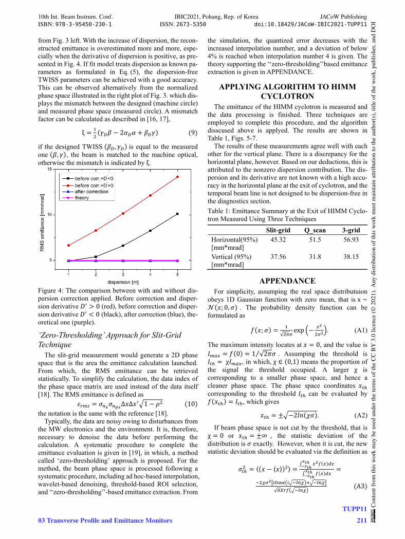
from Fig. 3 left. With the increase of dispersion, the recon-structed emittance is overestimated more and more, espe-cially when the derivative of dispersion is positive, as pre-sented in Fig. 4. If fit model treats dispersion as known pa-rameters as formulated in Eq. (5), the dispersion-free TWISS parameters can be achieved with a good accuracy. This can be observed alternatively from the normalized phase space illustrated in the right plot of Fig. 3. which dis-plays the mismatch between the designed (machine circle) and measured phase space (measured circle). A mismatch factor can be calculated as described in [16, 17],

ξ 𝛾 𝛽 2𝛼 𝛼 𝛽 𝛾 9

if the designed TWISS 𝛽 , 𝛾 is equal to the measured one 𝛽, 𝛾 , the beam is matched to the machine optical, otherwise the mismatch is indicated by ξ.

Figure 4: The comparison between with and without dis-persion correction applied. Before correction and disper-sion derivative 𝐷 0 (red), before correction and disper-sion derivative 𝐷 0 (black), after correction (blue), the-oretical one (purple).

‘Zero-Thresholding’ Approach for Slit-Grid Technique

The slit-grid measurement would generate a 2D phase space that is the area the emittance calculation launched. From which, the RMS emittance can be retrieved statistically. To simplify the calculation, the data index of the phase space matrix are used instead of the data itself [18]. The RMS emittance is defined as

𝜀 𝜎 𝜎 Δ𝑥Δ𝑥 1 𝜌 10 the notation is the same with the reference [18].

Typically, the data are noisy owing to disturbances from the MW electronics and the environment. It is, therefore, necessary to denoise the data before performing the calculation. A systematic procedure to complete the emittance evaluation is given in [19], in which, a method called ‘zero-thresholding’ approach is proposed. For the method, the beam phase space is processed following a systematic procedure, including ad hoc-based interpolation, wavelet-based denoising, threshold-based ROI selection, and ‘‘zero-thresholding’’-based emittance extraction. From

the simulation, the quantized error decreases with the increased interpolation number, and a deviation of below 4% is reached when interpolation number 4 is given. The theory supporting the ‘‘zero-thresholding’’based emittance extraction is given in APPENDANCE.

APPLYING ALGORITHM TO HIMM CYCLOTRON

The emittance of the HIMM cyclotron is measured and the data processing is finished. Three techniques are employed to complete this procedure, and the algorithm disscused above is applyed. The results are shown in Table 1, Figs. 5-7.

The results of these measurements agree well with each other for the vertical plane. There is a discrepancy for the horizontal plane, however. Based on our deductions, this is attributed to the nonzero dispersion contribution. The dis-persion and its derivative are not known with a high accu-racy in the horizontal plane at the exit of cyclotron, and the temporal beam line is not designed to be dispersion-free in the diagnostics section.

Table 1: Emittance Summary at the Exit of HIMM Cyclo-tron Measured Using Three Techniques

Slit-grid Q_scan 3-grid Horizontal(95%) [mm*mrad]

45.32 51.5 56.93

Vertical (95%) [mm*mrad]

37.56 31.8 38.15

APPENDANCE For simplicity, assumping the real space distributuion

obeys 1D Gaussian function with zero mean, that is x ∼𝒩 𝑥; 0,𝜎 . The probability density function can be formulated as

𝑓 𝑥;𝜎√

exp . (A1)

The maximum intensity locates at 𝑥 0, and the value is 𝐼 𝑓 0 1 √2𝜋𝜎⁄ . Assumping the threshold is 𝐼 χ𝐼 , in which, χ ∈ 0,1 means the proportion of the signal the threshold occupied. A larger χ is corresponding to a smaller phase space, and hence a cleaner phase space. The phase space coordinates 𝑥 corresponding to the threshold 𝐼 can be evaluated by 𝑓 𝑥 𝐼 , which gives

𝑥 2𝑙𝑛 𝜒𝜎 . (A2)

If beam phase space is not cut by the threshold, that is χ 0 or 𝑥 ∞ , the statistic deviation of the distribution is 𝜎 exactly. However, when it is cut, the new statistic deviation should be evaluated via the definition as

𝜎 ⟨ 𝑥 ⟨𝑥⟩ ⟩

√

A3



TUPP11

211

Con

tent

from

this

wor

km

aybe

used

unde

rthe

term

sof

the

CC

BY

3.0

licen

ce(©

2021

).A

nydi

stri

butio

nof

this

wor

km

ustm

aint

ain

attr

ibut

ion

toth

eau

thor

(s),

title

ofth

ew

ork,

publ

ishe

r,an

dD

OI

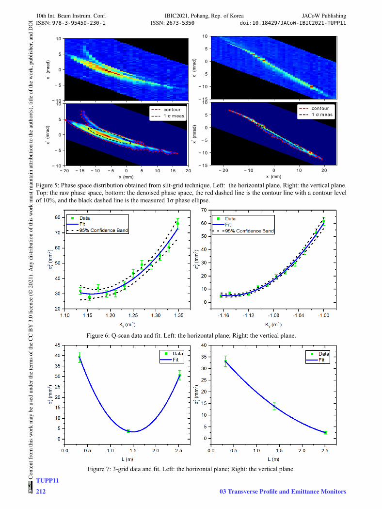
Figure 5: Phase space distribution obtained from slit-grid technique. Left: the horizontal plane, Right: the vertical plane. Top: the raw phase space, bottom: the denoised phase space, the red dashed line is the contour line with a contour level of 10%, and the black dashed line is the measured 1σ phase ellipse.

Figure 6: Q-scan data and fit. Left: the horizontal plane; Right: the vertical plane.

Figure 7: 3-grid data and fit. Left: the horizontal plane; Right: the vertical plane.


TUPP11Con

tent

from

this

wor

km

aybe

used

unde

rthe

term

sof

the

CC

BY

3.0

licen

ce(©

2021

).A

nydi

stri

butio

nof

this

wor

km

ustm

aint

ain

attr

ibut

ion

toth

eau

thor

(s),

title

ofth

ew

ork,

publ

ishe

r,an

dD

OI

212 03 Transverse Profile and Emittance Monitors

, in which 𝑖 is the complex, 𝐷𝑎𝑤 𝑥 ≡exp 𝑥 exp 𝑡 𝑑𝑡 is the Dawson’s integral,

𝐸𝑟𝑓 𝑧 ≡√

exp 𝑡 𝑑𝑡 is the Error function. The

ratio between 𝜎 and 𝜎 is

𝛿 𝜒√

. A4

The evolution of 𝛿 with χ is shown in Fig. 8. It is a monotonic decreasing function. The limit of 𝛿 𝜒 near the χ 0 is

lim→𝛿 𝜒 1 (A5)

, which indicates that 𝜎 approaches 𝜎 when χ approaches 0. It geives the correctness of the formulation Eq. (A4). With the increase of χ, a linear section occurs, which gives the possibility to approximate the 𝜎 with 𝜎 linearly. Series expansion of 𝛿 𝜒 at far away from χ 0 is

𝛿 𝜒 0.823 1.453 𝜒 0.1 𝒪 𝜒 0.1 . (A6)

Linear approximation gives a good estimation of 𝜎, as depicted in Fig. 8. Therein the dotted red line is a linear approximation of 𝛿 𝜒 . The deviation is large somewhat near the χ 0. The maximum deviation is 0.03, and the maximum deviation in terms of statistic deviation 𝜎 is less than 2%.

Figure 8: The evolution of 𝛿 with χ. Green line is 𝛿 𝜒 , dotted red line is a linear approximation.

REFERENCES [1] J. Yang et al., “Design of a compact structurecancer therapy

synchrotron”, Nucl. Instrum. Meth. A, vol. 756, pp. 19–22, 2014. https://doi.org/10.1016/j.nima.2014.04.050

[2] J. Shi et al., “Heavy ion medical machine (HIMM) slow ex-traction commissioning”, Nucl. Instrum. Meth. A, vol. 918, pp. 76–81, 2019. doi:10.1016/j.nima. .2018.11.014

[3] Y. C. Chen et al., “Optimization and Upgrade of Slow Ex-traction Control System for HIRFL CSR Main Ring”, in Proc. 16th Int. Conf. on Accelerator and Large Experi-mental Physics Control Systems (ICALEPCS'17), Barcelona, Spain, Oct. 2017, pp. 1663-1665. doi:10.18429/JACoW-ICALEPCS2017-THPHA122

[4] J. Montano et al., “Off-line emittance measurements of the SPES ion source at LNL”, Nucl. Instrum. Meth. A, vol. 648, pp. 238–245, 2011. doi:10.1016/j.nima.2011.05.038

[5] X.H. Wang, Z.G. He, and J. Fang, “Slit-based emittance measurement system for high-brightness injector at Hefei light source”, High Power Laser Part. Beams, vol. 24, pp. 457–462, 2012. doi:10.3788/HPLPB20122402.0457

[6] C. Xiao et al., “Measurement of the transverse four-dimen-sional beam rms-emittance of an intense uranium beam at 11.4MeV/u”, Nucl. Instrum. Meth. A, vol. 820, pp. 14-22, 2016. doi:10.1016/j.nima.2016.02.090

[7] F. Lohl et al., “Measurements of the transverse emittance at the FLASH injector at DESY”, Phys. Rev. Spec. Top. Accel. Beams, vol. 9, p. 092802, 2006. doi:10. 1103/PhysRevSTAB.9.092802

[8] M. Olvegard and V. Ziemann, “Effect of large momentum spread on emittance measurements”, Nucl. Instrum. Meth. A, vol. 707, pp. 114–119, 2013. doi:10.1016/j.nima.2012.12.114

[9] Z. Zhang and X.G. Jiang, “Pulsed intense electron beam emittance measurement”, Nucl. Sci. Tech., vol. 25, p. 060201, 2014. doi:10.13538/j.1001-8042/nst.25.060201

[10] L.Y. Zhang and J.J. Zhuang, “Calculation of two-screen emittance measurement”, Nucl. Instrum. Meth. A, vol. 407, pp. 356–358, 1998. doi:10.1016/S0168-9002(98)00049-7

[11] K. Levenberg, “A Method for the Solution of Certain Non-Linear Problems in Least Squares”, The Quarterly of Ap-plied Mathematics, vol. 2, pp. 164-168, 1944.

[12] D.W. Marquardt, “An algorithm for least-squares estimation of nonlinear parameters”, Journal of the Society for Indus-trial and Applied Mathematics, vol. 11(2), pp. 431-441, 1963.

[13] Mark K. Transtrum and James P. Sethna, “Improvements to the Levenberg-Marquardt algorithm for nonlinear least-squares minimization”, arXiv:1201.5885v1 [physics.data-an].

[14] X. Huang, S. Y. Lee, K. Y. Ng, and Y. Su, “Emittance meas-urement and modeling for the fermilab booster”, Phys. Rev. ST Accel. Beams, vol. 9 p. 014202, 2006. doi:10.1103/PhysRevSTAB.9.014202

[15] K. Holldack, J. Feikes, and W. Peatman, “Source size and emittance monitoring on BESSY II”, Nucl. Instrum. Meth. A, vol. 467, pp. 235-238, 2001. doi:10.1016/S0168-9002(01)00555-1

[16] M. G. Minty and F. Zimmermann, Measurement and Con-trol of Charged Particle Beams, Springer-Verlag Berlin Hei-delberg New York: Springer, 2003

[17] S. Y. Lee, Accelerator Physics (3thd Edition), Singapore: World Scientific, 2011.

[18] A. W. Chao et al., “Heavy Ion Linacs—Emittance Measure-ments P. Forck, P. Strehl”, in Handbook Of Accelerator Physics And Engineering (2nd Edition), Singapore: World Scientific, 2013, pp. 702-704.

[19] Y.-C. Feng et al., “Transverse emittance measurement for the heavy ion medical machine cyclotron”, Nucl. Sci. Tech., vol. 30(12), pp. 184, 2019. doi:10.1007/s41365-019-0699-7



TUPP11

213

Con

tent

from

this

wor

km

aybe

used

unde

rthe

term

sof

the

CC

BY

3.0

licen

ce(©

2021

).A

nydi

stri

butio

nof

this

wor

km

ustm

aint

ain

attr

ibut

ion

toth

eau

thor

(s),

title

ofth

ew

ork,

publ

ishe

r,an

dD

OI

emittance measurement algorithm and application to himm

Documents