emissions analysis routine for subsonic aircrafts using

Politecnico di Torino

Corso di Laurea Magistrale in Ingegneria Aerospaziale A.a. 2020/2021

Tesi di Laurea Magistrale Sessione di Laurea Ottobre 2021

Emissions analysis routine for subsonic aircrafts using biofuel

Relatori: Candidato: Nicole Viola Roberta Fusaro Davide Ferretto

Riccardo Biasco

2

Index

List of figures 1

List of tables 2

List of symbols 3

Introduction 4

Chapter 1 5

1 Aviation environmental impact and alternative fuels

1.1 Emissions from air transport 7

1.2 Actions for emission control and potential reduction 10

1.2.1 ICAO LTO cycle legislation 12

1.3 Biofuel, types, characteristics and production technologies 13

1.3.1 Biofuel production processes 15

1.3.2 Biofuel sources of supply 18

Chapter 2 22

2 Emissions calculation on mission profile: ICAO database and Fuel Flow method

II

2.1 ICAO data bank and LTO cycle prescriptions 23

2.2 ICAO database correction 25

2.2.1 Fuel flow correction 25

2.2.2 CO & Nox emission index correction 29

2.3 CO2 emissions calculation method 31

2.4 Fuel Flow Method 2 33

2.4.1 EI correction with altitude 36

2.4.2 Fuel Flow correction with altitude 39

2.4.3 Data interpolation and mission analysis 42

2.4.3.1 JET-A1 44

2.4.3.2 CSPK (100%) 45

2.4.3.3 JSPK (100%) 46

2.4.3.4 Results and discussion 47

3

Chapter 3 48

3 Icao database integration

3.1 Genetic gas generator performance analysis 48

3.2 Emission calculation with correlation based models 55

3.2.1 Nitrogen Oxides 55

3.2.2 Carbon dioxide and water 56

3.2.3 Carbon monoxide 56

3.2.4 Hydrocarbons 57

3.3 Example of calculation 58

Conclusions 64

Appendix A

Matlab code for Fuel Flow method application 65

Bibliography 80

1

List of Figures

Figure 1.1 Aviation Market forecast to 2050

Figure 1.2 Pollutant emissions in relation to fuel and air used for one hour of flight

Figure 1.3 Schematic Aviation Emissions Reduction Roadmap (IATA)

Figure 1.4 Life Cycle for kerosene and biofuel

Figure 1.5 German and Brasil arable land in comparison to land needed for biofuel

production

Figure 2.1 LTO cycle prescribed by ICAO in Annex 16 part II

Figure 2.2 Thrust, fuel flow and sfc for different blend of CSPK

Figure 2.3 Thrust, fuel flow and sfc for different blend of JSPK

Figure 2.4 Emissions characteristic curve CFM56-5°4 using JET-A

Figure 2.5 EICO LTO cycle for CFM56-5°4

Figure 2.6 EICO2 LTO cycle for CFM56-5°4

Figure 2.7 EIHC LTO cycle for CFM56-5°4

Figure 2.8 EINOx LTO cycle for CFM56-5°4

Figure 2.9 Gas generator scheme

Figure 2.10 Flow chart of the algorithm used to develop matlab code for emissions

calculations

Figure 3.1 Generic gas generator scheme

Figure 3.2 Thrust characteristics of typical aircraft engine

Figure 3.3 Specifications for General Electric CF6-50C2

Figure 3.4 Trend of the dosage f as a function of the end-of-combustion temperature

Figure 3.5 Emissions index related to F.F. for CO, CO2, HC and Nox for JET-A1

Figure 3.6 Emissions index related to T2 for CO, CO2, HC and Nox for JET-A1

Figure 3.7 Emissions index related to F.F. for CO, CO2, HC and Nox for CSPK

Figure 3.8 Emissions index related to T2 for CO, CO2, HC and Nox for CSPK

2

List of tables

Table 1.1 Summary of air traffic indicators

Table 1.2 Main emissions from the combustion process of aircraft engines and

corresponding radiative forcing

Table 1.3 Different type of biofuel and carbon emission reduction

Table 1.4 JSPK and CSPK chemical and phisical properties

Table 2.1 Biofuel properties

Table 2.2 Thrust, fuel flow and sfc for different blend of CSPK

Table 2.3 Thrust, fuel flow and sfc for different blend of JSPK

Table 2.4 Emission index CO correction [%]

Table 2.5 Emission index Nox correction [%]

Table 2.6 Emission index for CFM International CFM56-5A4 (Airbus A-320), for

different type of fuel

Table 2.7 Input parameters for mission profile simulation

Table 3.1 Data and results of simulation for CF6-50C2 using Jet-A1

Table 3.2 Data and results of simulation for CF6-50C2 using CSPK

4

Introduction

Air transport is an ever-expanding sector, it carries goods and people on a daily basis and

represents the most efficient and fastest means of connection in today's world. However, it has

limitations; it is necessary, together with technological development, to evaluate different

methodologies of approach to the problems arising from the environmental impact.The

emissions forecast for the coming years, in parallel with the growth forecast for the sector, make

it necessary to search for valid alternatives to reduce and control the amount of substances

emitted into the atmosphere. One of these lies in the use of alternative fuels with high efficiency

and low environmental impact, for the related life cycle. Among the most popular, due to their

peculiarities, there are biofuels.

This research aims to provide a method for assessing the pollutants emitted by air transport and

resulting from the use not only of traditional fuels, but also of alternative fuels (drop-in

biofuels). Specifically, with the use of pre-existing methods and studies and with the

implementation of new calculation algorithms, it is possible to analyze the emissions deriving

from a complete flight, modulated phase by phase according to the individual characteristics of

a complete mission profile. In order to be able to make the survey iterative, a code in Matlab

language has been developed that is capable of carrying out the analysis with the only request

of entering some input data.

The first chapter provides an overview of the current and future needs of air transport, growth

forecasts and the impact they could have on the environment. The issues relating to the

emissions of chemical compounds deriving from the combustion processes of aeronautical

engines are discussed and the fuels obtained from biomass are presented in broad terms,

focusing on the sources from which they can be obtained, on the production processes and

finally on the chemical and physical characteristics of the same. An overview is thus provided

which will be characterized in the second chapter by a more accurate description of the

peculiarities of the fuels, this time focused on the performance characteristics and the

corresponding emission index. A model is also proposed for calculating emissions at high

altitude and in general with varying flight conditions. This method is closely linked to the ICAO

emissions databank, from which it derives some fundamental parameters. In the case in which

it is necessary to disengage from the database, in chapter 3, an alternative model is proposed

that exploits empirical relationships to obtain the emission indexes, together with the

application of some basic equations of gas dynamics and the application of the performance

analysis on design of the aeronautical engine. Finally, in the appendix, the Matlab code

generated to complete the simulations and analyzes is proposed and made available.

5

Chapter 1

Aviation environmental impact and alternative fuels

In 2017, airlines around the world carried around 4.1 billion passengers, 56 million tons of

cargo on 37 million commercial flights. Every day, airplanes carry over 10 million passengers

and approximately $ 18 billion in goods. Aviation provides the world's only rapid transit

network, generating economic growth, creating jobs and facilitating international trade and

tourism. Over the course of the twentieth century, aviation has evolved to become one of the

most influential industries on the planet. The sector is constantly growing, and judging by the

studies of the International Civil Aviation Organization (ICAO), the trend is practically

exponential.

Figure 1.1 Aviation Market forecast to 2050

6

Together with the increase in flights and fleets, if the situation remained unchanged from a

technological point of view, there would be a dizzying increase in airborne pollutants. In 2016,

aviation was responsible for 3.6% of total emissions of green house gas (GHG, main responsible

for the greenhouse effect) within the European Union and 13.4% of emissions attributable to

transport alone.1

From figure 1.1 and table 1.1 it is possible to see how the aviation market is destined for

constant growth. The growing trend is also evident in the data obtained from the European

Aviation Safety Agency (EASA), and specifically in the IATA (International Air Transport

Association) indicators. Year after year, the number of short, medium and long-haul flights, the

number of passengers, the quantities of goods, the distances traveled and the number of airlines,

as well as the number of fleets and aircraft per fleet, increase with growth rates of over 50% in

some cases. It is therefore necessary and in the common interest to address the issue of

sustainability in order to mitigate the environmental impact of the sector.

Table 1.1 Summary of air traffic indicators2

1 European aviation environmental report, Colonia, 2019, EASA 2 European aviation environmental report, Colonia, 2019, EASA

7

1.1 Emissions from air transport

Aircraft emit a range of gases and particles which affect the atmosphere. In the context of

climate change, the major emissions are CO2, nitrogen oxides (NOx), water vapour (H2O),

sulphur oxides (SOx) and soot. A summary of the atmospheric impacts of these agents and

estimates of their associated radiative forcings in 2000 is provided in Table 1.2 Radiative

forcing is a measure of the impact of an agent on the energy balance of the earth’s atmosphere.

It is technically defined as the change in net irradiance at the tropopause (i.e. the boundary

between the troposphere and stratosphere) and is measured in watts per square metre (W/m2).

A positive number indicates the agent has a warming effect, a negative number indicates a

cooling agent.

Table 1.2 Main emissions from the combustion process of aircraft engines and corresponding radiative forcing

8

According to the data reported by the member states of the United Nations Framework

Convention on Climate Change (UNFCCC), the annual carbon dioxide emissions of all flights

operating in the areas of the European Union increased by 95% - from 88 to 171 million tons -

between 1990 and 2016. Future emissions, according to the same studies, will vary by + 21%

in 2040, or reaching 198 million tons. Similarly, the nitrogen monoxide produced in flight

annually increased from 313,000 to 700,000 tons from 1990 to 2016, and is expected to reach

1000000 tons in 20403. The amount of these emissions, which contribute to the greenhouse

effect, obviously contribute to the rise in the average earth temperature, with disastrous and

well-known consequences on the ecosystem. It is estimated by the Intergovernmental Panel on

Climate Change (IPCC) that by the year 2100 the world will see a temperature change of 2.5–

7.8 °C above the average for the years between 1850 and 19004.

The effects of emissions into the atmosphere can be grouped into three macro categories5:

- Direct GHG emissions (CO2 and H2O).

Combustion of fossil fuel results in the formation of CO2 gas which is typically released

as engine emissions. For every kilogram of fuel burned, 3.155 kg of CO2 are formed. It

is accepted within the scientific community that these fossil fuel emissions have resulted

in increases in atmospheric CO2 levels6.

arbon dioxide is a gas with high thermodynamic and photochemical stability, and

consequently is highly durable over time (100 years) Nowadays, CO2 emissions from

the aviation sector alone constitute 2% of all emissions anthropogenic and 10-13% of

emissions deriving from transport in general7. Another element of considerable

importance is water vapor H2O, which contributes to global warming. However, the

vapor emissions attributable to air transport are negligible compared to those from other

sources, such as evaporation from the earth's surface, and also typically the vapor is

disposed of in a couple of weeks by precipitation. If these emissions are released at an

altitude lower than that of the tropopause, they do not constitute a substantial problem,

precisely because the time spent in the atmosphere is, as already mentioned, short;

- Emissions that can contribute to the formation of GHG (NOx and CO).

The nitrogen oxides produced by aviation make up 2% of the total anthropogenic

production. The residence time of the molecule varies with altitude: in the vicinity of

the tropopause it is 10 times greater than that of the soil. It is usually converted into

ammonia HNO3 after weeks. This causes a considerable influence on the chemical

balance of the atmosphere. Reactions that have nitrogen oxides and carbon monoxide

as reactants can also generate ozone O3 as a secondary product. The latter, if present in

3 European aviation environmental report, Colonia, 2019, EASA 4 L. Zhang., T. L. Butler, B. Yang, Recent Trends, Opportunities and Challenges of Sustainable Aviation Fuel, Green Energy to Sustainability: Strategies for Global Industries, ed. 1, 2020 John Wiley & Sons Ltd., 2020 5 M. Shaefer, Methodologies for aviation emissions calculation – A comparison of alternative approaches towards 4D global inventories, Berlin University of Technology, German Aerospace Center (DLR), 2006 6 D. Daggett, Enabling Alternate Fuels for Commercial Aircraft, Cranfield University, 2009 7 Intergovernmental Panel on Climate Change: Aviation and Global Atmosphere, Cambridge university press, 1999

9

the stratosphere, acts as a screen for UV radiation, but at lower altitudes it is in effect a

green hous gas with a lifetime of the order of weeks;

- Substances or particulates that influence the formation and properties of clouds

The combustion inside aircraft engines produces, together with the other elements, soot

and sulphate particles. These are negligible compared to the quantities emitted to the

ground by other phenomena such as volcanic eruptions; however, their concentration in

the atmosphere could influence the generation of ozone, modify the properties of the

clouds, their composition and contribute to the formation of cirrus clouds. These are all

phenomena that contribute to the greenhouse effect;

Figure 1.2 Pollutant emissions in relation to fuel and air used for one hour of flight

10

1.2 Actions for emission control and potential reduction

In 2010, the member states drew up an agreement, through the ICAO, with the intention of

increasing the average efficiency of the fuels used by 2% per year, or reducing emissions and

imposing a maximum tolerable limit on them. In 2012, an action plan was signed for the first

time to outline the policies and guidelines to be universally followed to reduce the impact of

aviation on the climate. The initiative of 2012 is followed by that of 2016. In October 2016, the

International Civil Aviation Organization (ICAO) stated the new requirements in the Carbon

Offsetting and Reduction Scheme for International Aviation (CORSIA) (ICAO’s 39th

Assembly 2016). CORSIA is an international scheme for regulating CO2 emissions from Civil

Aviation. Its goal is to have a carbon neutral growth from 2020. CORSIA uses Market-based

environmental policy instruments to offset CO2 emissions: aircraft operators have to

purchase carbon credits8 from the carbon market. Starting in 2021, the scheme is voluntary for

all countries until 2027.

At the moment, aviation is not yet one of the main drivers of global warming, but the surge in

the growth trajectory of the sector suggests that it could become the decisive factor in the

coming decades.9

Sustainable mobility is an essential element for social and economic maintenance and

development. Air transport must therefore support economic growth by providing a means

capable of creating connections while respecting the prerogatives of an eco-sustainable system.

The Advisory Council for Aviation Research and Innovation in Europe (ACARE) has set 5

"goals of flightpath 2050" in order to be able to provide members some guidelines on which to

develop future projects, again for the only purpose of ensuring sustainable development:

- The technologies and procedures available in the sector must guarantee a reduction of

CO2 emissions per passenger / km of 75% and a reduction of nitrogen oxide emissions

of 90%;

- Taxi maneuvers must guarantee zero emission index;

- Airplanes will be designed and built to be as recyclable as possible;

- Europe will have to establish itself as a center of excellence for the research and use of

sustainable alternative fuels, including those for aviation, on the basis of a strong

European energy policy;

- Europe must be at the forefront of atmospheric impact research and must take the lead

in formulating a priority environmental action plan and in defining global environmental

standards;

Obviously, in order to achieve these objectives set for 2050, the configuration and operation of

aircraft will need to be gradually and significantly changed.10

8 A carbon credit or carbon credit is a negotiable certificate, or a security equivalent to one ton of CO2 not emitted or absorbed thanks to an environmental protection project carried out with the aim of reducing or reabsorbing global emissions of CO2 and other greenhouse gases. 9 A. Macintosh, L. Wallace, International Aviation Emissions to 2025: can emissions be stabilised without restricting domand?, Canberra, 2008, pp 5-6 10 Strategic research and innovation agenda, 2017 update, Advisory Council for Aviation Research and Innovation in Europe, Derby, 2017, pp 48-60

11

It is essential in today's landscape to carry out research and optimize the times in order to

provide new methodologies for approaching the problem of environmental sustainability. To

make possible the objectives set for the near future, it is necessary to improve and integrate the

existing systems and known technologies. Aviation, as suggested by ACARE, can reduce CO2

emissions by improving the efficiency of fuel, technology, operations and infrastructure, but

also by making it possible to use alternative and sustainable fuels (as in the case of biofuels ,

which will be discussed later). Fuel efficiency is widely discussed, a factor that indicates the

average fuel consumption usually referred to a single passenger per kilometer. If this value is

not increased, as required, by at least 2% per annum, the scenario generated will see a drastic

increase in airborne pollutants, a greater demand for fuel in parallel with the growing trend of

air transport and a consequent increase in medium prices.

It is therefore in the interest of the aeronautical industry to evaluate alternative fuels that can at

the same time increase fuel efficiency and ensure an energy source that does not come from

traditional fossil fuels. So the interest of the aviation industry stems from:

- Generation of additional sources;

- Potential cost reduction;

- Environmental advantages;

12

1.2.1 ICAO LTO cycle legislation

Aircraft engines must comply with the emission standards defined by ICAO in annex 16 volume

2. These regulations contain a limit imposed on the maximum emissions of pollutants, and

specifically CO, HC, Nox and soot during a predetermined landing cycle. and take off (LTO).

As an integral part of the certification process, manufacturers must provide data relating to

performance characteristics and emissions. All data is made available and public through the

ICAO engine exhaust emissions databank.

Specifically, the emissions for each phase are provided by means of an emission index, i.e. in

the form of grams of pollutant emitted per kg of fuel burned (fuel consumption is also supplied

in kg / s units).

The ICAO standards were generated mainly to have local air quality control available near

airports. Therefore, as anticipated, they only concern taxi operations, take offs, climb and

landing, i.e. operations that take place below 3000 ft.

Universal standards are also defined for the characteristic thrust of each phase, as well as for

the duration of the same. Emissions at high altitudes are omitted from the certification process,

and a method for their estimation, together with the requirements for the individual phases, will

be presented in the following chapters.

The fuel flow is used to calculate the total gross emissions 𝐷𝑝 of each pollutant during the entire

LTO cycle. Thrust specific value 𝐷𝑝 𝐹∞⁄ in g/kN is the relationship between the big missions

and the maximum thrust of the engine, and is used as a parameter for the imposition of the

upper limits of certification11:

- Regulatory smoke number:

83.6 ∙ (𝐹∞)−0.274

- Regulatory HC level:

𝐷𝑝

𝐹∞= 19.6 [

𝑔

𝑘𝑁]

- Regulatory CO level

𝐷𝑝

𝐹∞= 118 [

𝑔

𝑘𝑁]

- Regulatory Nox level:

different value, dependent on date of production, maximum thrust and overall pressure

ratio;

11 Environmental Protection, Annex 16, Vol. II, International Civil Aviation Organization, 3 ed., 2008

13

1.3 Biofuel, types, characteristics and production

technologies

The aviation industry uses specific fuels to power thrusters, and these are usually classified as

JET-A1 fuels. All fuels must strictly comply with certain specifications, wirh ASTM providing

the most common standards worldwide, also including the category of renewable and

sustainable fuels.

A suistainable alternative fuel can be described as one without negative environmental,

economic, and social impacts. In addition to having lower lifecycle green house gas (GHG)

emissions, sustainable biofuel should not compete with food or fresh water resources or

contribute to deforestation, while providing socioeconomic value to local communities where

plant stocks are grown. Oil base energy crops that can meet these sustainability criteria

include, but are not limited to jatropa, camelina and algae. Based on the recent results of well-

to-wheel12 Life Cycle Assessments (LCA) carried out by Michigan Technological University,

Bio-SPK (Synthetic Paraffinic Kerosene) made from jatropa and camelina oils can achieve a

reduction of GHG emissions between 65 and 80 percent relative to petroleum derived jet fuel13.

Therefore biofuels can potentially reduce GHG emissions and the consequent impact on climate

change compared to traditional fossil fuels if we refer to a complete well to wheel life cycle

analysis (fig. 1.4).

Achieving the pollutant reduction targets set as targets by international organizations such as

the ICAO requires, in view of the use of biofuels for this purpose, an increase in their production

and consumption.

Biofuels may theoretically be produced from any type of biomass, i.e. renewable living

organism utilizing carbon as a food source. However, the production of biofuels mostly comes

from the processing of grasses, plant seeds, and non-edible tree fruits. As a matter of fact,

contrary to fossil sources, biomass sources absorb carbon dioxide as they grow in a proportion

equivalent to that produced when the fuel is burnt in the jet engine. As a consequence, when the

extraction of fossil fuels releases large amounts of CO2 in the atmosphere, the growth of

biomass feedstocks absorbs large amounts of CO2. This absorption sometimes more than

compensates the remaining lifecycle CO2 emissions associated with the production of

biofuels.14

12 Well to wheel: it allows to compare fuels for energy analysis and can be used for environmental analysis. The primary objective of this index is to compare different propulsion technologies and fuels with each other. The comparison takes place by relating the effectiveness of the means of transport, the performance of the technology that makes it possible to obtain the fuel and the energy carrier used both to transport it and to store it. 13 J. D. Kinder, T. Rahmes, Evaluation of bio-derived synthetic paraffinic kerosene (Bio-SPK), The boeing Company, Sustainable Biofuels Research & Technology Program, 2009 14 A. P. Payan, M. Kirby, C. Y. Justin, D. N. Mavris, Meeting Emissions Reduction Targets: A Probabilistic Lifecycle Assessment of the Production of Alternative Jet Fuels, in American Institute of Aeronautics and Astronautics, School of Aerospace Engineering, Georgia Institute of Technology, Atlanta, 2015

14

Current fuel consumption for the entire international aviation sector according to ICAO

estimates of 2016 could reach 852 million tons in 2050; and approximately 426 million tons of

biofuels would be needed to achieve the objectives set for GHG reduction. However, current

production is very small and limited, managing to cover 1% of aircraft fuel consumption

worldwide15.

Figure 1.3 Schematic Aviation Emissions Reduction Roadmap (IATA)16

Figure 1.4 Life Cycle for kerosene and biofuel

15 Beginners guide to aviation biofuel, Air Transport Action Group, 2009 16 The IATA technology roadmap report, IATA, 3rd Edition, Montreal, QC, Canada, 2013

15

The vast majority of biofuels currently available are derived from oleochemical feedstocks (an

oleochemical is a chemical compound derived industrially from animal or vegetable oil or fats)

such as vegetable oil, animal fat and used cooking oil (UCO).

A further significant advantage in the use of biofuels, regardless of the potential reduction of

pollutants and the low environmental impact of their production process, lies in the fact that

they can be used on pre-existing aircraft configurations, without the need to make changes.

They are called "drop in" fuels. A “drop-in jet fuel blend” is a substitute for conventional jet

fuel, that is completely interchangeable and compatible with conventional jet fuel when blended

with conventional jet fuel. A drop-in fuel blend does not require adaptation of the

aircraft/engine fuel system or the fuel distribution network, and can be used “as is” on currently

flying turbine-powered aircraft.17

1.3.1 Biofuel production processes

In May 2016, the American Society for Testing and Materials (ASTM) certified four different

processes that can be used for the production of biofuels. As is known, obtaining such a

certification affects the possibility of exploiting this technology for powering commercial and

international flights.

The certification referred to is the ASTM standard D7566 and officially recognizes 4 production

processes:

- Hydroprocessed Esters and Fatty Acids (HEFA bio-jet), are derived from oleochemical

feedstocks. They represent the basic concept of biofuels, and were certified in 2011;

- Gasification through the Fischer-Tropsch method (FT), using urban organic waste

(MSW) or biomass. It is a high temperature biomass treatment process for the

production of a gas which is then used to generate synthetic hydrocarbon fuels over

catalysts;

- Synthesised Iso-Paraffinic fuels (SIP). It is a process that involves the fermentation of

sugars through microorganisms to create a hydrocarbon molecule called farnesene,

which in turn, treated with hydrogen, produces farnesane which is the actual fuel to be

blended with JET-A;

- Alcohol-to-jet like the SIP it provides for a fermentation process of sugars in alcohols

such as ethanol or buthanol and has been certified in 2016;

Nowadays, the majority of bio-fuels currently on the market are HEFA, also because the process

used is similar to that used for the production of diesel for road transport and beyond, so several

facilities benefit from this production technology.

17 Sustainable aviation fuels guide, ICAO, 2017

16

In total, in 2016 the total amount of the global HEFA fuel production capacity was around 4.3

billion liters per year. And if we hypothesize to use this quantity only for the aeronautical

market we would be able to cover only 1.5% of the needs of the sector.

One of the reasons why the presence of biofuels is so low in the sector is the cost of production.

HEFA fuels have a price that is higher than that of traditional fossil fuels as in the management

costs, in addition to production, it is necessary to consider the maintenance prices of the

plantations from which the raw materials are obtained. As an example, in 2016 the cost of palm

oil (which is the cheapest of all) was 0.45 USD / L, while the price of aviation fuel 0.25 USD /

L, practically half. To overcome this problem, several governments (such as Netherlands,

Norway, U.S.) are moving towards the implementation of specific policies in order to make it

possible to reduce spending on plantation maintenance and conversion processes18. And it will

be precisely these policies that establish the feasibility or otherwise of the objectives set for

2050. In recent years, the number of biofuel-powered commercial flights has increased

significantly and a downstream supply chain has been developed in some locations.

Another of the current limits to the large-scale use of these fuels is the lack of mature production

technology. The HEFA process has been present for several years and for this reason more

developed, but the cost of the raw material, or biomass obtained from plantations, is too high

and constitutes 80% of the cost of the fuel itself.

A table (1.3) is shown on the next page, obtained from an EASA report, which highlights the

peculiarities of the main biofuels, differentiating them according to the technology adopted for

the production process. Specifically, the percentages of possible reductions in carbon dioxide

emissions are highlighted.

18 D. Daggett, O. Hadaller, R. Hendricks, R. Walther, Alternative Fuels and their Potential Impact on Aviation, NASA, October 2006

17

Table 1.3 Different type of biofuel and carbon emission reduction

18

1.3.2 Biofuel sources of supply

Biofuels, as mentioned above, are mainly derived from plants, and can be considered

sustainable energy sources if a sufficient amount of crops can be grown to meet the demand19.

Unfortunately, several regions or states would not have adequate production capacity,

especially in relation to the areas available to be exploited by crops, to meet their own energy

needs. For example, the figure below shows that the land available for cultivation in Germany

covers 34% of the entire surface of the state.

Figure 1.5 German and Brasil arable land in comparison to land needed for biofuel production

To meet the demand for fuel of the same nation, attested to around 56.6 million tons in 200520,

with an equal amount in energy terms of biofuels, a arable area 4 times larger than that currently

available would be needed, in addition to the complete replacement of all the crops currently

present. However, the situation is quite different in other geographical areas, where the

available surface is far greater than that necessary to satisfy the demands of the market, such as

Brazil.

Replacing kerosene on a large scale in the aeronautical sector is by no means easy and it is a

challenge that various governments have been working on in recent years. As an example,

consider that even the global use of blends at 15% by volume of biofuels in JET-A1 is currently

impossible. In 2006, the US commercial fleet used approximately 51.5 billion liters of fuel over

the course of a year. 15% of annual consumption would correspond to 7.72 billion liters of

biofuel. Furthermore, considering that a plantation such as soybean (widely present in the

United States) produces about 225 liters of biofuel for each acre (0.0556 l/ 𝑚2), 34 million

acres of arable land would be needed, or about the entire area of Florida (140 billion 𝑚2)21.

19 Useful information about conventional and alternate fuels and their feedstocks, National Renewable Energy Lab, National Bioenegineering Center, june 2004 20 Lieberz, S., Germany Oilseeds and Products, Biodiesel in Germany – An Overview, USDA Report #GM2021, October 24, 2002 21 D. Daggett, O. Hadaller, R. Hendricks, R. Walther, Alternative Fuels and their Potential Impact on Aviation, NASA, October 2006

19

Renewable feedstocks are the best raw material from which to start the production of biofuels.

The fundamental characteristics of these sources reside in:

- Sustainability;

- Carbon dioxide recycling;

- Renewability;

- Eco-friendly technology;

- Less dependence on petroleum supplying countries;22

Generically favored sources are derived from crops, plantations, organic waste, forest residuals

and halophytes. Among the main ones, the main ones used for the production of biofuel, in

relation to their characteristics are:

- CAMELINA

It is a plant widely used for the production of vegetable oil, thanks to its seeds containing

a high oil content. The oil content varies between 30 and 40%, and is also a plant that

does not need fertilizers for growth, can be grown on poorly fertile soils and is not

affected by diseases and insects. The remains resulting from the extraction of the oil can

be safely used as animal feed. Furthermore, the production costs, for the reasons listed

above, are reduced compared to other crops, and are around 0.10-0.20 $ / l. In 2012,

around 750 million liters of oil were produced in the United States.

-JATROPHA

Like the camelina plantations, the jatropha is a plant species that can grow in marginal

land, not very fertile soils, it is a resistant plant and little affected by parasites. It grows

rapidly in geographic areas with a favorable climate. However, the waste produced by

obtaining the oil cannot be used in the food industry or on farms as it is poisonous, but

at the same time it can be exploited for the extraction of nitrogen, sodium and potassium.

- ALGAE

They constitute a valid alternative to remedy the current scarce provision of other

sources and vast arable land. They have a high lipid content, a high carbon dioxide

absorption rate during their life cycle, low land take and a high growth rate.

The most influential positive side lies in the fact that they do not affect and do not

conflict with other pre-existing crops since they do not require the availability of land

and especially water for their cultivation.

The remaining biomass as a result of oil extraction can be used for food purposes, as

feed for intensive farming, for the production of paper and bioplastics and again for the

production of energy.

- WASTES

The waste, as such, comes from different sources, and can be converted into biofuels

following different procedures. They are a widely present and economic resource.

22 Bozel JJ. The use of renewable feedstocks for the production of chemicals and materials-a brief overview of concepts

20

Furthermore, usually, above all, municipal organic waste is rich in fats and therefore are

suitable for the extraction of oils.

- HALOPHYTES

They are herbs that grow in salty waters, and in environments hostile to other plant

species. They are usually readily available in tropical and subtropical areas. Also in this

case there is no need to have arable land and moreover, as in the case of algae, obviously

they do not require the addition of water, consequently the production costs are very

low.

Due to the previous advanced knowledge of production technology and the current level of

progress, for this research, it was decided to focus attention on HEFA biofuels, and in particular

on those obtained from camelina and jatropha.

The latter choice is linked to the vast availability of information in this regard, such as the

chemical properties of the fuel obtained from them with the above methodology.

Hydroprocessed renewable jet fuels (HRJs) anche detti hydroprocessed esters and fatty acids

(HEFA) are typically paraffinic liquids with molecular formula 𝐶𝑛𝐻2𝑛+2, they are produced by

hydrodeoxygenation of vegetable oils and animal fats, and most of the by-products are made

up of water and propane. This category of fuels is peculiar for their high combustion energy

efficiency and for the possibility of being exploited even in the absence of a second element /

mixing fuel. They are free of aromatics and sulfur, have a high thermal stability. They can be

used without having to modify the architecture of the engines, they prevent the formation of

deposits and corrosion of the constituent elements of the engine, and their combustion is ash

free, they retain good properties even at low temperatures, which is why they can also be used

at high altitudes. Finally, the molecules are devoid of oxygen.23

Below is a table that lists the main characteristics and specifications of the fuels taken into

consideration. In the following chapters, a detailed analysis of the performance characteristics

deriving from the use of the aforementioned biofuels on aircraft engines is dealt with

23 Hari, Yaakob, Binitha, Aviation biofuel from renewable resources: routes, opportunities and challenges, renewable and suistenable energy reviews, 2015

21

Table 1.4 JSPK and CSPK chemical and phisical properties

Properties Jatropha Camelina

Density [kg/m^2] 864-880 780

Cetane number 46-55 50.4

Viscosity [mm^2/s @40°C] 3.7-5.8 3.8

Pour Point [°C] 5 -7

Flash Point [°C] 163-238 136

Lower Heating Value [MJ/kg] 44.4 44

CFPP [°C] -1.2 -3

Acid Value [mg/KOH] 0.34 -

Cloud Point [°C] 5 3

Oxidation Stability [h] 5 -

Iodine Value [I2/100g] 109.5 152.8

Sulphur Content [ppm] 12.9 -

Specific Gravity [g/ml] 0.876 0.882

Molecular Formula C12H26 C12H24.5

22

Chapter 2

Emissions calculation on mission profile: ICAO

database and Fuel Flow method II

The purpose of this work is to obtain an estimate of the emissions of pollutants as the parameters

of a mission profile vary. The method used to base this estimate is the fuel flow method 2. For

its correct application, however, it is necessary to know in advance the emissions values at sea

level, in order to then be able to make a correction based on the change in altitude applied to

the calculation of the fuel flow rate in the different flight conditions. For this purpose, the ICAO

databank provides a valid source from which obtaining the emission values at zero altitude,

however its limit lies in the unavailability of data relating to the use of non-traditional fuels.

Consequently, following previous studies on the characteristics and performance of biofuels, a

predictive estimate of the pollutants generated by them is made, thus expanding the availability

of data contained in the ICAO database.

The application of the different methods together allows to obtain an estimate of the emission

indexes for CO CO2 NOx and HC in the different phases of the mission profile, moment by

moment, and finally an estimate of the total emissions during the entire flight envelope.

The calculation algorithm that summarizes the procedure followed to obtain the results

discussed in the next chapter is presented below.

1) Obtaining corrective factors for 𝐸𝐼𝑠𝑙 and 𝑤𝑓 𝑠𝑙 resulting from the use of biofuels;

2) Expansion of the ICAO database with the inclusion of new types of fuel and

corresponding performance characteristics;

3) Application of fuel flow method to obtain EI and 𝑤𝑓 in different flight conditions;

4) Iteration of the fuel flow method to obtain emissions along the entire mission profile;

23

2.1 ICAO Annex 16: databank and LTO cycle prescriptions

The issue of the environmental impact of aircraft is included in Annex 16 of the Chicago

Convention, wich is in force in countries belonging to the ICAO – International Civil Aviation

Organization. Mentioned ICAO Annex 16 contains 2 parts: the first concerns at emissions and

the second one is about aircraft noise. The emissions parts include the description of the

metodology for assessing emission of harmful exhaust compounds from civil aircraft engines

by universal LTO test (Landing and Take-off). 24

This test is a mapping of the operations carried out near the airports, i.e. taxiing, take off,

climbing and approaching. For the case of civil aviation, the ICAO directives provide for a

different thrust configuration for each phase:

- Take off T=100% Tmax

- Climb out T=85% Tmax

- Approach T=30% Tmax

- Taxi T=7% Tmax

The reference emissions LTO cycle for the calculation and reporting of gaseous emissions are

represented by the following time in each operating mode. Phase Time in operating mode25:

- Take off t=0.7 min

- Climb out t=2.2 min

- Approach t=4 min

- Taxi t=26 min

Figure 2.1 LTO cycle prescribed by ICAO in Annex 16 part II

24 M. Nowak, R. Jasinski, M. Galant, Implementation of the LTO cycle in flight conditions using FNPT II MCC simulator, in IOP Conference series: materials science and engineering, pp 1-3 25 Annex 16: Environmental protection, vol II: Aircraft Engine Emissions, 4th ed., ICAO

24

The emissions obtained according to the LTO test is defined as the mass of harmful compound

per mass of fuel used in the test. It is esoressed as the mass of compounds in 1g referred to

1000g of consumed fuel.

A generalized emission characterization for each single phase is presented in summary.

- Take off: the phase is characterized by the lower quantity of HC and CO, but at the same

time by the maximum values of NOx which are the result of the high temperatures in

the combustion chamber;

- Climb: it differs slightly from the initial take off phase. In fact, the thrust is reduced by

only 15%, as well as all the other performance parameters, slightly reduced. This

guarantees a negligible variation in emissions;

- Approach and landing: emissions of carbon monoxide and unburnt hydrocarbons are

higher than in the climb and take off phases due to the lower temperature of the

combustion process;

- Taxi: the phase is characterized by a longer duration than the other phases and at the

same time by the maximum values of HC and CO emitted. This makes this phase the

most significant from the point of view of emissions within the entire LTO cycle;

Engine manufacturers generally carry out tests for certification and monitoring of polluting

emissions by varying the performance of the same from minimum to maximum power,

simulating the entire possible spectrum of flight regimes. However, the data obtained from these

tests are not made public by the certification bodies and manufacturing companies, except in

small quantities. Specifically, these are 4 characteristic points used in the calculations for

obtaining the certification corresponding to the LTO duty cycle. These data are in practice those

reported in the ICAO database. Although the inclusion in the data bank is entirely voluntary,

most of the certified engines are present there, starting from 1982, the year in which the ICAO

Emissions Standards were officially adopted.

So the International Civil Aviation Organization (ICAO) Engine Emissions Databank contains

information, voluntarily provided by manufacturers, on exhaust emissions of production

aircraft engines, measured according to the procedures in ICAO Annex 16 Vol II, and where

noted, certified by their States of Design as implemented in their national regulations. This

Databank contains information on only those engines that have entered production, irrespective

of the numbers actually produced. It has been compiled mainly from information supplied for

newly certified engines.

25

2.2 ICAO database correction

The data in the ICAO database, as anticipated, refer to tests conducted on engines fueled with

traditional JET-A fuel. This work aims to analyze the emissions resulting from the use of

biofuels. It is therefore necessary to make changes to the existing database, creating a parallel

one referring to the new fuel class.

In the literature there are several studies on the performance characteristics of gas generators of

aircraft engines. The results are presented below and refer to both the correction of the fuel flow

and the correction of the emission indices.

2.2.1 Fuel Flow correction

A study by the University of Cranfield examined the effects of the variation in calorific value

(heat capacity) and fuel density on the performance of the propulsion system in terms of thrust

and fuel consumption26. The influence of heat capacity and density was studied by simulating

the use of a biofuel in a high bypass ratio turbofan using a tool / software developed in house

called Pythia. Pythia is a software developed about 30 years ago by the University of Cranfield,

capable of carrying out analyzes on the performance of aircraft engines of any type both in

project conditions and in over-project conditions.

Two main types of biofuels were considered:

- Jatropa bio-synthetic paraffinic Kerosene, abbreviated JSPK, with molecular formula

𝐶12𝐻26

- Camelina bio-synthetic paraffinic kerosene, abbreviated CSPK, with molecular formula

𝐶12𝐻24.5;27

In order to exploit the data obtained experimentally from this previous study, the analysis in its

entirety will henceforth be developed with reference only to these two types of fuel.

26 Effects of biofuels properties on aircraft engine performance, in Aircraft Engineering and aerospace technology, 87(5), pp 437-443, Emerald, 2013 27 Muhammad Hanafi Azami, M. Savill, Comparative study of alternative biofuels on aircraft engine performance, in Journal of Aerospace Engineering, vol. 231, 2017, pp 1509-1521

26

Table 2.1 Biofuel properties

Properties Jatropha Camelina

Density [kg/m^2] 864-880 780

Cetane number 46-55 50.4

Viscosity [mm^2/s @40°C] 3.7-5.8 3.8

Pour Point [°C] 5 -7

Flash Point [°C] 163-238 136

Lower Heating Value [MJ/kg] 44.4 44

CFPP [°C] -1.2 -3

Acid Value [mg/KOH] 0.34 -

Cloud Point [°C] 5 3

Oxidation Stability [h] 5 -

Iodine Value [I2/100g] 109.5 152.8

Sulphur Content [ppm] 12.9 -

Specific Gravity [g/ml] 0.876 0.882

Molecular Formula C12H26 C12H24.5

The fuels considered were used both in pure form and in the form of a mixture in different

percentages with traditional JET-A fuels, and to be exact in blends at 20, 40, 60, 80 and 100%.

The purpose of the research is precisely to evaluate the effects and establish a relationship

between the percentage of blend used and the performance of the propulsion system.

Tables 3.1 and 3.2 show the percentage variation in engine thrust, fuel consumption and SFC,

calculated for the various biofuel blends (CSPK and JSPK respectively), comparing these

values to those obtained through the use of traditional JET fuel. Specifically, compared to JET-

A, both biofuels show an increase in thrust and fuel flow, but a reduction in the SFC, despite

the latter being negligible.

The data obtained from this study were used to obtain a corrective coefficient to be applied for

the correction of the fuel flow in the ICAO database tables, as, as is well known, this makes

available only and exclusively data obtained from experimental tests on aero engines powered

by JET-A. It is therefore assumed that the performance or behavior of each engine broadly

reflects that of the model used for the simulation using the PYTHIA software.

27

Table 2.2 Thrust, fuel flow and sfc for different blend of CSPK

BLEND THRUST FUEL FLOW SFC

20% 0.02 -0.49 -0.49

40% 0.04 -0.78 -0.82

60% 0.07 -1.09 -1.15

80% 0.1 -1.38 -1.47

100% 0.12 -1.69 -1.8

Table 2.3 Thrust, fuel flow and sfc for different blend of JSPK

BLEND THRUST FUEL FLOW SFC

20% 0.01 -0.6 -0.61

40% 0.03 -1.03 -1.05

60% 0.05 -1.46 -1.5

80% 0.07 -1.88 -1.94

100% 0.09 -2.31 -2.39

Figure 2.2 Thrust, fuel flow and sfc for different blend of CSPK

28

Figure 2.3 Thrust, fuel flow and sfc for different blend of JSPK

Once the corrective factors have been obtained to be able to modify the fuel flow made available

in the ICAO database, which we recall refers only and exclusively to the combustion of Jet-A1

fuel, it is necessary to find a method to calculate the emissions of pollutants, and specifically of

CO, NOx and HC, in relation to the use of biofuels.

As previously mentioned in this research it was decided to analyze only HEFA CSPK and JSPK

fuels.

29

2.2.2 Emission index correction

B. Gawron, T. Bialecki et al.28 stimate the emissions resulting from the use of biofuels.

Specifically, reference is made to HEFA CAM and UCO. CAM stands for Camelina, so it is

the equivalent of the CSPK; as for the UCO EFAs, on the other hand, they are biofuels obtained

from cooking oil. It was therefore necessary at this point to compare the properties of the latter

with those of the JSPK, in order to justify the replacement within the analysis. The data obtained

shows a remarkable similarity between the two categories of biofuels, in terms of density,

combustion efficiency and lower heating value, which is why it was considered appropriate to

exploit the data obtained experimentally from the combustion of UCO, assuming similar

characteristics and results for the JSPK.

The study derived percentage corrective factors to be applied to the data already present related

to the use of traditional fuel. The discussion neglects the variation of unburned hydrocarbons,

which is why their value will be kept constant during the subsequent analysis. Each simulation

of the aforementioned study, aimed at obtaining the emission indices, is carried out at different

rotational speed values of the engine, each related to the different thrust configurations

characteristic of each phase of the LTO cycle. As the rotational speed and consequently the

thrust of the engine increase, it is evident how the emissions of carbon monoxide are reduced,

while the emissions of nitrogen oxides and carbon dioxide are increasing.

Tables 3.4 and 3.5 summarize the research results that will be applied in order to create an

extension of the ICAO database for CSPK and JSPK biofuel cases

Table 2.4 Emission index CO correction [%]

IDLE APPROACH CRUISE TAKEOFF

CSPK 50% -6 -8.5 -0.5 11

CSPK 20% -2.4 -3.4 -0.2 4.4

CSPK 40% -4.8 -6.78 -0.4 8.8

CSPK 60% -7.2 -10.2 -0.6 13.2

CSPK 80% -9.6 -13.6 -0.8 17.6

CSPK 100% -12 -17 -1 22

JSPK 50% -4 -7 -6 0.2

JSPK 20% -1.6 -2.8 -2.4 0.08

28B. Gawron, T. Bialecki, A. Janicka, T. Suchocki, Combustion and Emissions Characteristics of the turbine engine fueled with HEFA Blends from different feedostock, in Energies, vol. 1277, 2020, pp 1-12

30

JSPK 40% -3.2 -5.6 -4.8 0.16

JSPK 60% -4.8 -8.4 -7.2 0.24

JSPK 80% -6.4 -11.2 -9.6 0.32

JSPK 100% -8 -14 -12 0.4

Table 2.5 Emission index Nox correction [%]

IDLE APPROACH CRUISE TAKEOFF

CSPK 50% 21.8 17.5 15 10.5

CSPK 20% 8.72 7 6 4.2

CSPK 40% 17.44 14 12 8.4

CSPK 60% 26.16 21 18 12.6

CSPK 80% 34.88 28 24 16.8

CSPK 100% 43.6 35 30 21

JSPK 50% 11.5 9.5 7.9 4.9

JSPK 20% 4.6 3.8 3.16 1.96

JSPK 40% 9.2 7.6 6.32 3.92

JSPK 60% 13.8 11.4 9.48 5.88

JSPK 80% 18.4 15.2 12.64 7.84

JSPK 100% 23 19 15.8 9.8

31

2.2.3 CO2 emissions calculation method

In the ICAO database there are no references regarding the production and emissions of carbon

dioxide. For this reason it was necessary to find in the literature a method suitable for

calculating the aforementioned emissions.

For this purpose it was assumed to use the COPERT model29. This estimates the emissions

generated by road transport and internal combustion engines. Although this model may seem

inappropriate at first sight, it differentiates between types of pollutants, which allows us to

exploit it even in the aeronautical case in the case of carbon dioxide emissions.

The model of calculating the exhaust emissions differs on the basis of the identification of four

groups of pollutants:

- Group 1: CO, NOx, COV, CH4, COVNM, N2O, NH3 e PM. For these pollutants,

specific emission factors linked to the different conditions of the engine and to the

operating cycles are used;

- Group 2: CO2, SO2. The emissions of these pollutants are estimated solely on the basis

of fuel consumption;

- Group 3: IPA, PCDD e POP. On these pollutants no detailed data is available and a

simplified methodology is used;

- Group 4: pollutants obtained as a fraction of total NMVOC emissions;

Obviously, the group of interest for the purposes of this request is Group 2, which makes it

possible to estimate CO2 emissions. And, as previously mentioned, although this refers to a

model developed for road transport, it can also be used on an aeronautical model as it is based

solely and exclusively on the combustion process, on the molecular characteristics of the fuel

and on its consumption.

So for the purposes of calculating CO2 emissions, it is assumed that the carbon content of the

fuel is oxidized to 99% into CO2. If the composition of the fuel is known, denoting by c, h and

o the mass fractions of the carbon, hydrogen and oxygen atoms, with c+h+o=1, the ratios

between hydrogen and carbon and between oxygen and carbon in the fuel are respectively equal

to:

𝑟𝐻:𝐶 = 11.916ℎ

𝑐

𝑟𝑂:𝐶 = 0.7507𝑜

𝑐

29 A. Bernetti, R. De Lauretis, G. Iarocci, F. Lena, R. Marra Campanale, E. Taurino, Inventario nazionale delle emissioni e disaggregazione provinciale, Istituto Superiore per la Ricerca e Protezione Ambientale, 2010

(2.1)

(2.2)

32

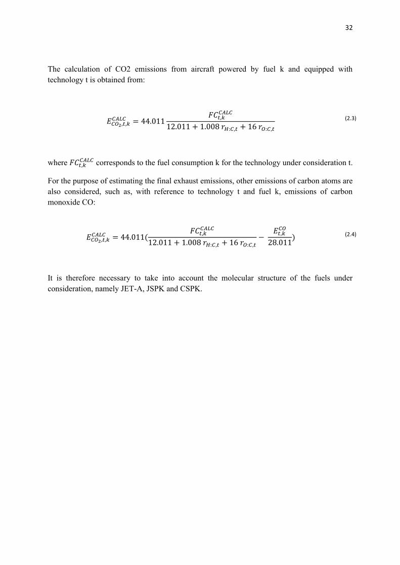
The calculation of CO2 emissions from aircraft powered by fuel k and equipped with

technology t is obtained from:

𝐸𝐶𝑂2,𝑡,𝑘𝐶𝐴𝐿𝐶 = 44.011

𝐹𝐶𝑡,𝑘𝐶𝐴𝐿𝐶

12.011 + 1.008 𝑟𝐻:𝐶,𝑡 + 16 𝑟𝑂:𝐶,𝑡

where 𝐹𝐶𝑡,𝑘𝐶𝐴𝐿𝐶 corresponds to the fuel consumption k for the technology under consideration t.

For the purpose of estimating the final exhaust emissions, other emissions of carbon atoms are

also considered, such as, with reference to technology t and fuel k, emissions of carbon

monoxide CO:

𝐸𝐶𝑂2,𝑡,𝑘𝐶𝐴𝐿𝐶 = 44.011(


12.011 + 1.008 𝑟𝐻:𝐶,𝑡 + 16 𝑟𝑂:𝐶,𝑡−

𝐸𝑡,𝑘𝐶𝑂

28.011)

It is therefore necessary to take into account the molecular structure of the fuels under

consideration, namely JET-A, JSPK and CSPK.

(2.3)

(2.4)

33

2.3 Obtaining characteristics curves

Table 3.6 shows part of the database thus obtained. Specifically, it was decided to report the

performance characteristics to varying the type of fuel for a single type of engine, purely by

way of example (CFM International CFM56-5A4). Regardless of this, obtaining the emission

values and fuel flow rates for each individual phase of the cycle, allows to obtain characteristic

curves (Fig. 3.4), which will be exploited in the subsequent part of the analysis.

The data will be interpolated through the values obtained from the fuel flow, allowing the

analysis of emissions at high altitude. By exploiting the a priori knowledge of the relationship

between EI and fuel flow in the different flight phases, thanks to the data obtained from the

ICAO database, it is possible to represent first degree curves.

By way of example, the graph obtained using the characteristics of the CFM56-5A4 engine

powered by traditional Jet fuel for the purposes of the simulation is shown. As mentioned

previously, CO and HC have a maximum value in the taxi phase and a decreasing trend with

increasing fuel flow. Conversely, opposite behavior for CO2 and NOx.

Figure 2.4 Emissions characteristic curve CFM56-5A4 using JET-A

34

Table 2.6 Emission index for CFM International CFM56-5A4 (Airbus A-320), for different type of fuel

As previously said about the ICAO regulations, it is possible to obtain the emission trend during

an entire LTO cycle by considering not only the values present in the database but also the

FuelJET A1 CSPK 20% CSPK 40% CSPK 60% CSPK 80% CSPK 100%JSPK 20% JSPK 40% JSPK 60% JSPK 80% JSPK 100%

Rated Thrust (kN)97.89 97.89 97.89 97.89 97.89 97.89 97.89 97.89 97.89 97.89 97.89

HC EI T/O (g/kg)0.23 0.23 0.23 0.23 0.23 0.23 0.23 0.23 0.23 0.23 0.23

HC EI C/O (g/kg)0.23 0.23 0.23 0.23 0.23 0.23 0.23 0.23 0.23 0.23 0.23

HC EI App (g/kg)0.5 0.5 0.5 0.5 0.5 0.5 0.5 0.5 0.5 0.5 0.5

HC EI Idle (g/kg)1.75 1.75 1.75 1.75 1.75 1.75 1.75 1.75 1.75 1.75 1.75

CO2 T/O kg/s2.7807 2.7999 2.7918 2.7831 2.7749 2.7662 2.7969 2.7848 2.7727 2.7609 2.7488

CO2 C/O kg/s2.294 2.3099 2.3032 2.296 2.2892 2.282 2.3073 2.2974 2.2874 2.2776 2.2676

CO2 App kg/s0.8091 0.7147 0.8123 0.8098 0.8074 0.8049 0.8138 0.8103 0.8068 0.8033 0.7998

CO2 Idle kg/s0.2945 0.2965 0.2957 0.2947 0.2939 0.293 0.2962 0.2949 0.2937 0.2924 0.2911

CO EI T/O (g/kg)1.1 1.1484 1.1968 1.2452 1.2936 1.342 1.0088 1.1018 1.1026 1.1035 1.1044

CO EI C/O (g/kg)1.1 1.0978 1.0956 1.0934 1.0912 1.089 1.0736 1.0472 1.0208 0.9944 0.968

CO EI App (g/kg)3.1 2.9946 2.8892 2.7838 2.6784 2.573 3.0132 2.9326 2.8396 2.7528 2.666

CO EI Idle (g/kg)20.3 19.8128 19.3256 18.8384 18.3512 17.864 19.9752 19.6504 19.3256 19.0008 18.676

NOx EI T/O (g/kg)22.64 23.5909 24.5418 25.4926 26.4435 27.3944 23.0837 23.5275 23.9712 24.415 24.8587

NOx EI C/O (g/kg)19.11 20.2566 21.4032 22.5498 23.6964 24.843 19.7139 20.3178 20.9216 21.5255 22.1294

NOx EI App (g/kg)8.51 9.1057 9.7014 10.2971 10.8928 11.4885 8.8334 9.1568 9.4801 9.8035 10.1269

NOx EI Idle (g/kg)4.04 4.3923 4.7446 5.0969 5.4492 5.8014 4.2258 4.4117 4.5975 4.7834 4.9692

Fuel Flow T/O (kg/sec)0.897 0.8926 0.89 0.8872 0.8846 0.8818 0.8916 0.8878 0.8839 0.8801 0.8763

Fuel Flow C/O (kg/sec)0.74 0.7364 0.7342 0.7319 0.7298 0.7275 0.7356 0.7324 0.7292 0.7261 0.7229

Fuel Flow App (kg/sec)0.261 0.2597 0.259 0.2582 0.2574 0.2566 0.2594 0.2583 0.2572 0.2561 0.2549

Fuel Flow Idle (kg/sec)0.095 0.0945 0.0943 0.094 0.0936 0.0933 0.0944 0.094 0.0936 0.0932 0.0928

Ambient Baro Min (kPa)94.7 94.7 94.7 94.7 94.7 94.7 94.7 94.7 94.7 94.7 94.7

Ambient Baro Max (kPa)95.6 95.6 95.6 95.6 95.6 95.6 95.6 95.6 95.6 95.6 95.6

Ambient Temp Min (K)280 280 280 280 280 280 280 280 280 280 280

Ambient Temp Max (K)291 291 291 291 291 291 291 291 291 291 291

Humidity Min (kg/kg)0.0026 0.0026 0.0026 0.0026 0.0026 0.0026 0.0026 0.0026 0.026 0.026 0.026

Humidity Max (kg/kg)0.0034 0.0034 0.0034 0.0034 0.0034 0.0034 0.0034 0.0034 0.0034 0.034 0.034

35

requirements regarding the duration of each individual phase. The following pages show the

graphs relating to emissions of CO (fig. 3.5), CO2 (fig. 3.6), HC (fig. 3.7), and Nox (fig. 3.8).

Figure 2.5 EICO LTO cycle for CFM56-5°4 Figure 2.6 EICO2 LTO cycle for CFM56-5°4

Figure 2.7 EIHC LTO cycle for CFM56-5°4 Figure 2.8 EINOx LTO cycle for CFM56-5°4

36

2.4 Fuel flow method 2

At this point, after having obtained the emission indices relating to a standard LTO cycle, a

method must be adopted that guarantees the possibility of carrying out the assessment as flight

conditions vary, thus allowing to obtain an estimate of the emissions of pollutants while

cruising, at high altitude and in general along an entire mission profile. For this purpose, the

Fuel Flow Method 2 is used30.

The recent scenarios, discussed extensively in the previous chapters, have led to the

aeronautical sector the need to quantify the emissions generated by aeroengines. The main and

best known method in the sector for the calculation of NOx HC and CO is the so-called "P3T3".

Although not as rigorous as the P3T3, the Fuel Flow Method represents a valid alternative for

emissions certification. This method can offer an approximation of the emissions with nominal

calculated values characterized by an error of 10-15% compared to those obtained with the

traditional P3T3.

The P3T3 requires knowledge of the evolution of the parameters inside the engine, and in

particular through the high pressure compressor and the combustor diffuser. The parameters

under consideration are the total pressure p3 (in this treatment p2), and the total temperature T3

(in this treatment T2), the input parameters in the combustor, the fuel flow rate wf. Furthermore,

for the sole purpose of calculating the emissions of nitrogen oxides, it is also necessary to know

the relative humidity of the environment. This information is then fed into a model that

evaluates the performance of the machine. It is evident that not all the information necessary to

carry out the analysis using the P3T3 method can be easily found, and some of them can only

be obtained through the proprietary performance model. As a consequence of this, methods

with a simplified approach have been proposed, based solely on the dependence on the flow

rate of fuel in the combustion chamber wf such as fuel flow. However, for the correct

application of the latter, knowledge of the typical emission indices of the LTO cycle is required,

usually provided after the ICAO certification process.

The method used is presented below, and is divided into two fundamental parts: the first aims

to obtain a correction of the emission indices as the altitude varies, the second instead is useful

for obtaining a relationship that allows to correct the value of fuel flow with altitude.

30 D. Dubois, G. C. Paynter, Fuel Flow Method 2 for estimating Aircraft emissions, The Boeing Company, SAE international, 2006

37

2.4.1 Emission index correction with altitude

It is assumed that the compression process between the combustor inlet and the air intake is

isentropic:

𝑇2

𝑇1= (

𝑝2

𝑝1)

𝛾−1𝛾

𝑇2 = 𝑇1(𝑝2

𝑝1)

𝛾−1𝛾

Figure 2.94 Gas generator scheme

Writing the equation to the flight conditions:

𝑇2 𝑎𝑙𝑡 = 𝑇1 𝑎𝑙𝑡(𝑝2 𝑎𝑙𝑡

𝑝1 𝑎𝑙𝑡)

𝛾−1𝛾

and at seal level

𝑇2 𝑠𝑙 = 518.67(𝑝2 𝑠𝑙

14.696)

𝛾−1𝛾

Furthermore it can be assumed that

𝑇2 𝑠𝑙 = 𝑇2 𝑎𝑙𝑡

Taking advantage of this last relationship, and joining it to the previous ones, we obtain:

(2.5)

(2.6)

(2.7)

(2.8)

(2.9)

38

𝑇1 𝑎𝑙𝑡(𝑝2 𝑎𝑙𝑡

𝑝1 𝑎𝑙𝑡)

𝛾−1𝛾 = 518.67(

𝑝2 𝑠𝑙

14.696)

𝛾−1𝛾

Which can be rewritten as

𝑝2𝑎𝑙𝑡

𝑝2 𝑠𝑙=

𝛿1

𝜃1

𝛾−1𝛾

A beta coefficient is now introduced which takes into account the ratio between total and static

quantities, such that

𝛽 = 1 +𝛾 − 1

2𝑀

2

You can then write that

𝑝2 𝑎𝑙𝑡

𝑝2 𝑠𝑙=

𝛿𝑎𝑚𝑏 𝛽𝛾

𝛾−1

(𝜃𝑎𝑚𝑏 𝛽)𝛾

𝛾−1

=𝛿𝑎𝑚𝑏

𝜃𝑎𝑚𝑏

𝛾𝛾−1

And considering γ=1.4 for air

𝑝2 𝑎𝑙𝑡

𝑝2 𝑠𝑙=

𝛿𝑎𝑚𝑏

𝜃𝑎𝑚𝑏1.5

If a polytropic efficiency is used to describe the compression between sections 2 of the

combustor inlet and 1 of the air intake, then the relationship between pressures and temperatures

becomes

𝑇2

𝑇1= (

𝑝2

𝑝1)

𝛾−1𝜂𝑝𝛾

And considering γ=1.38 e 𝜂𝑝 = 90%

𝑝2 𝑎𝑙𝑡

𝑝2 𝑠𝑙=

𝛿𝑎𝑚𝑏

𝜃𝑎𝑚𝑏1.3

A small further empirical correction is then made

𝑝2 𝑎𝑙𝑡

𝑝2 𝑠𝑙=

𝛿𝑎𝑚𝑏1.02

𝜃𝑎𝑚𝑏1.3

Substituting this result in the equations of the P3T3 model, we obtain:

𝐸𝐼𝐶𝑂𝑎𝑙𝑡 = 𝐸𝐼𝐶𝑂𝑠𝑙(𝜃𝑎𝑚𝑏

3.3

𝛿𝑎𝑚𝑏1.02 )𝑥

(2.10)

(2.11)

(2.12)

(2.13)

(2.14)

(2.15)

(2.16)

(2.17)

(2.18)

39

𝐸𝐼𝐻𝐶𝑎𝑙𝑡 = 𝐸𝐼𝐻𝐶𝑠𝑙(𝜃𝑎𝑚𝑏

3.3


𝐸𝐼𝑁𝑂𝑥𝑎𝑙𝑡 = 𝐸𝐼𝑁𝑂𝑥𝑠𝑙(𝜃𝑎𝑚𝑏

3.3


The exponents x and y, in the absence of further indications, are usually set at 1 and 0.5

respectively.

2.4.2 Fuel flow correction with altitude

By writing the energy balance equation to the combustor, a corrective factor for the fuel flow

rate can be obtained

𝜂𝑏𝑤𝑓𝐿𝐻𝑉 = (𝑤𝑓 + 𝑤𝑎)𝐶𝑝(𝑇3 − 𝑇2)

Since the fuel flow is typically less than 2% of the total air flow, and furthermore if both the air

flow and the fuel flow are assumed to be at the same temperature, i.e. T2, and have the same

heat specific, a simplification can be made and the equation can be rewritten as

𝜂𝑏𝑤𝑓𝐿𝐻𝑉 = 𝑤𝑎𝐶𝑝(𝑇3 − 𝑇2)

Applying this equation at altitude and at sea level, and assuming that the temperatures T3

and T2 remain unchanged with the altitude

𝑤𝑓 𝑠𝑙 = 𝑤𝑓 𝑎𝑙𝑡

𝑤𝑎 𝑠𝑙

𝑤𝑎 𝑎𝑙𝑡

𝜂𝑏 𝑎𝑙𝑡

𝜂𝑏 𝑠𝑙

The air flow in the combustor at sea level can be written as

𝑤𝑎 𝑠𝑙 = 𝑘𝑝2 𝑠𝑙

√𝑇2 𝑠𝑙

𝑓(𝑀2)𝑠𝑙

where

𝑘 = √𝛾

√𝑅 𝑇3

And the Mach function takes the form

𝑓(𝑀3)𝑠𝑙 = 𝑀(1

𝛾 − 12 𝑀2 + 1

)𝛾+1

2(𝛾−1)

(2.19)

(2.20)

(2.21)

(2.22)

(2.23)

(2.24)

(2.25)

(2.26)

40

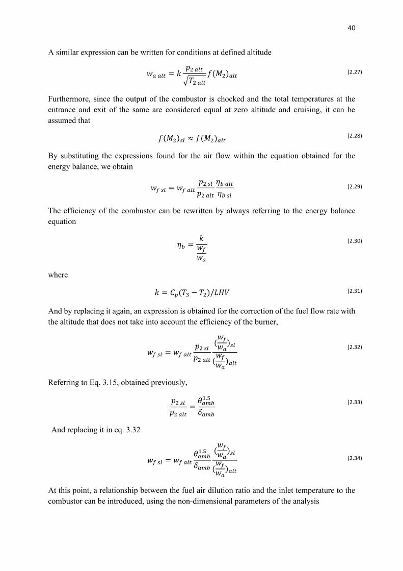
A similar expression can be written for conditions at defined altitude

𝑤𝑎 𝑎𝑙𝑡 = 𝑘𝑝2 𝑎𝑙𝑡

√𝑇2 𝑎𝑙𝑡

𝑓(𝑀2)𝑎𝑙𝑡

Furthermore, since the output of the combustor is chocked and the total temperatures at the

entrance and exit of the same are considered equal at zero altitude and cruising, it can be

assumed that

𝑓(𝑀2)𝑠𝑙 ≈ 𝑓(𝑀2)𝑎𝑙𝑡

By substituting the expressions found for the air flow within the equation obtained for the

energy balance, we obtain


𝑝2 𝑠𝑙

𝑝2 𝑎𝑙𝑡

𝜂𝑏 𝑎𝑙𝑡

𝜂𝑏 𝑠𝑙

The efficiency of the combustor can be rewritten by always referring to the energy balance

equation

𝜂𝑏 =𝑘

𝑤𝑓

𝑤𝑎

where

𝑘 = 𝐶𝑝(𝑇3 − 𝑇2)/𝐿𝐻𝑉

And by replacing it again, an expression is obtained for the correction of the fuel flow rate with

the altitude that does not take into account the efficiency of the burner,


𝑝2 𝑠𝑙

𝑝2 𝑎𝑙𝑡

(𝑤𝑓

𝑤𝑎)𝑠𝑙

(𝑤𝑓

𝑤𝑎)𝑎𝑙𝑡

Referring to Eq. 3.15, obtained previously,

𝑝2 𝑠𝑙

𝑝2 𝑎𝑙𝑡=

𝜃𝑎𝑚𝑏1.5

𝛿𝑎𝑚𝑏

And replacing it in eq. 3.32


𝜃𝑎𝑚𝑏1.5

𝛿𝑎𝑚𝑏

(𝑤𝑓

𝑤𝑎)𝑠𝑙

(𝑤𝑓


At this point, a relationship between the fuel air dilution ratio and the inlet temperature to the

combustor can be introduced, using the non-dimensional parameters of the analysis

(2.27)

(2.28)

(2.29)

(2.30)

(2.31)

(2.32)

(2.33)

(2.34)

41

𝑇2 𝑠𝑙 =𝑇2 𝑎𝑙𝑡

𝜃1

(𝑤𝑓

𝑤𝑎)𝑠𝑙 =

(𝑤𝑓


𝜃1

Then is introduced a corrective factork ,assumed constant,

(𝑤𝑓


𝜃1= 𝑘(

𝑇2 𝑠𝑙

𝜃1)𝑥

This last equation can also be rewritten at sea level,

(𝑤𝑓

𝑤𝑎)𝑎𝑙𝑡 = 𝑘(𝑇2 𝑠𝑙)

𝑥

And comparing the two relations (at altitude and at sea level), again considering the constant

T3 as the altitude varies,

(𝑤𝑓

𝑤𝑎)𝑠𝑙 = (

𝑤𝑓

𝑤𝑎)𝑎𝑙𝑡𝜃1

𝑥−1

Now, replacing the equation obtained within the relationship for calculating the fuel flow rate

at sea level (eq. 3.34)


𝜃𝑎𝑚𝑏3.5

𝛿𝑎𝑚𝑏𝜃1

𝑥−1

From experimental data the exponent x is fixed equal to 2 and consequently it is obtained:


𝜃𝑎𝑚𝑏3.5

𝛿𝑎𝑚𝑏𝜃1

Considering then compressible flow function relationships fot total to static pressure and

temperature,

𝜃1 = 𝜃𝑎𝑚𝑏(1 +𝛾 − 1

2𝑀2)

Replacing 𝜃1, and γ=1.4, eq. 3.41 will be


𝜃𝑎𝑚𝑏3.5

𝛿𝑎𝑚𝑏𝜃𝑎𝑚𝑏(1 + .2𝑀2)

From perturbation theory,

𝑒0.2𝑀2≈ (1 + .2𝑀2)

(2.35)

(2.36)

(2.37)

(2.38)

(2.39)

(2.40)

(2.41)

(2.42)

(2.43)

(2.44)

42

We can therefore write that


𝜃𝑎𝑚𝑏4.5

𝛿𝑎𝑚𝑏𝑒0.2𝑀2


𝜃𝑎𝑚𝑏3.8

𝛿𝑎𝑚𝑏𝑒0.2𝑀2

2.4.3 Data interpolation and mission analysis

The fuel flow allows first of all to obtain the fuel flow rate above sea level (eq. 3.46) knowing

the fuel flow rate at altitude. This relationship, together with the characteristic curves of

paragraph 3.4, will make it possible to calculate, by interpolation, the corresponding emissions

referring to sea level. Subsequently, thanks to relations 2.18, 2.19 and 2.20, it will be possible

to obtain the final result, that is the emissions of pollutants in the different flight conditions,

different from those of the LTO cycle.

Again by way of example, and referring to the previously reported case of the CFM56-5A4

engine, a complete analysis of the emissions along the typical mission profile of an Airbus

A320 is provided below, which is summarized in the table, together with the parameters entered

in input and required to perform the calculation. The code used to carry out the simulations is

contained in Appendix A, and consists of a series of iterative calculations, which instant by

instant calculate the emissions of compounds as the flight conditions vary by interpolating the

characteristic curves obtained from the database and the corrections presented above. Figure

2.10 shows a summary diagram of the calculation algorithm, highlighting inputs, outputs and

processes.

Table 2.7 Input parameters for mission profile simulation

IDLE TAKE OFF CLIMB CRUISE APPROACH LANDING

Max speed (M) 0.05 0.23 0.5 0.7 0.4 0.2

Max altitude [m] 0 1000 10000 10000 10000 1000

Min altitude [m] 0 0 1000 10000 1000 0

Time [s] 1200 60 120 3600 600 120

Fuel flow [kg/s] 0.01 0.9 0.7 0.5 0.3 0.2

(2.45)

(2.46)

43

Figure 2.10 Flow chart of the algorithm used to develop matlab code for emissions calculations

Three different simulations are then carried out in order to highlight the difference relating to

the use of different types of fuels. The first case sees the use of JET-A1, the second CSPK and

the third JSPK.

In the initial phase, a twin-engine configuration is set with a maximum thrust of the aircraft

equal to 200 kN; the results presented subsequently will therefore not refer to the performance

of the single engine, but to the entire propulsion system, thus representing a complete analysis

of the emissions generated by a short-haul flight (1.5 hours of operating cycle).

N.B in the histograms on the following pages: 1=taxi, 2=takeoff, 3=climb, 4=cruise,

5=approach, 6=landing.

44

2.4.3.1 JET-A1

45

2.4.3.2 CSPK (100%)

46

2.4.3.3 JSPK (100%)

47

2.4.3.4 Results and Discussion

It is evident that in the cases analyzed the greatest contribution of pollutants is to be attributed

to the cruise phase. This is not so much linked to the performance characteristics of the aircraft,

as to the time set for the aforementioned phase; for the simulation a time of 3600 sec has been

set (1h) for the cruise only, while all the other phases are typically of shorter duration. By

focusing on the total quantities of pollutants generated by the combustion of the three different

types of fuels, comparing kerosene and biofuels, for the latter it is possible to observe a

substantial reduction in the emissions of carbon dioxide, unburnt hydrocarbons and an icrease

nitrogen oxides, while it is a slight increase in the generation of carbon dioxide (albeit

negligible) is noticeable. Nevertheless, the advantage of using biofuels lies not so much in the

CO2 limitations related to its practical use as an oxidizer, as in the entire extraction and

production cycle, as widely described in chapter 1. Below are the histograms relating to the

production of compounds obtained from the above simulation.

48

Chapter 3

Icao database integration

The method presented in the following pages is designed for the occurrences in which it is

desired to carry out analysis of emissions by categories of engines that are not present in the

ICAO databank. It is therefore necessary to be able to obtain emission indices in order to expand

the existing database. It should be noted that the resulting indices refer to the pre-established

flight conditions and therefore do not always coincide with the SL conditions. Furthermore,

only and exclusively the cases in which the propulsion system operates in ON-DESIGN

conditions are considered. Considering the multitude of existing engines, and the variety of

them, the performance characteristics are analyzed for the gas generator group, which unites all

types of propulsion systems.

3.1 Generic gas generator performance analysis

The proposed alternative method aims at calculating the emissions of pollutants for those

engines not contained in the ICAO database and on which, not knowing the characteristics of

the respective LTO cycles -in terms of pollutants-, it is not possible to apply the fuel flow

method 2 previously proposed.

Specifically, by analyzing the performance on design of the engine, it is possible to obtain the

values of 𝑇2° and 𝑃2

° and then replace them in the appropriate relations for the calculation of

NOx, CO, CO2 and HC. In literature, these variables are indicated with 𝑇3° and 𝑝3

° for a

different denomination of the stages of the gas generator.

The starting point is the thermal balance in the combustion chamber, by equating the

corresponding enthalpy difference between sections 2 and 3 (inlet and outlet of the combustor)

and the thermal power:

𝑤𝑓𝐻𝑖𝜂𝑏 = (𝑤𝑓 + 𝑤𝑎)𝑐𝑝′ (𝑇3

° − 𝑇2°) (3.1)

49

Figure 3.1 Generic gas generator scheme

Subsequently, the factor 𝛼 can be introduced equal to the ratio between the air flow rate entering

the combustor 𝑤𝑎 and the fuel flow rate 𝑤𝑓, obtaining:

𝜂𝑏𝐻𝑖

(1 + 𝛼)𝑐𝑝′ = 𝑇3

° − 𝑇2°

Where 𝑇2° is the total temperature in the combustion chamber inlet equivalent to the temperature

leaving the compression stage and instead 𝑇3° is the temperature leaving the combustor, and

will be the degree of freedom of the system.

The specific heat 𝑐𝑝′ of the fluid after combustion can be expressed as:

𝑐𝑝′ = 𝑐�̅� +

1+𝛼𝑠𝑡

1+𝛼(54.818 + 0.7535𝑇𝑚

° )

𝑐�̅� = 946 +0.1844

2(𝑇3

° + 𝑇2°)

Where 𝑐�̅� is an average, approximate value. Substituting the relation 4 into the 3 we obtain:

𝑐𝑝′ = 946 +

0.1844

2(𝑇3

° + 𝑇2°) +

1 + 𝛼𝑠𝑡

1 + 𝛼[54.818 + 0.07535 (

𝑇3° + 𝑇2

°

2)]

𝑐𝑝′ = 𝑇3

° (0.1844

2+ 0.037675

1 + 𝛼𝑠𝑡

1 + 𝛼) + 𝑇2

° (0.1844

2+ 0.037675

1 + 𝛼𝑠𝑡

1 + 𝛼) + 946 + 54.818

1 + 𝛼𝑠𝑡

1 + 𝛼

(3.2)

(3.3)

(3.5)

(3.4)

(3.6)

50

At this point, for the sake of simplicity, a coefficient k is introduced, the terms of which can be

considered constant even when the environmental conditions vary

𝑘 =0.1844

2+ 0.03765

1 + 𝛼𝑠𝑡

1 + 𝛼

Obtaining a simplified expression for the specific heat at the end of the combustion process

𝑐𝑝′ = 𝑘𝑇3

° + 𝑘𝑇2° + 946 + 54.818

1 + 𝛼𝑠𝑡

1 + 𝛼

Relation 2 is now reported, resulting from the heat balance in the combustor

𝜂𝑏𝐻𝑖

(1 + 𝛼)= 𝑇3

°𝑐𝑝′ − 𝑇2

°𝑐𝑝′

And the expression 8 is replaced in the 9, developing the products

𝜂𝑏𝐻𝑖

(1 + 𝛼)= 𝑇3

° [𝑘𝑇3° + 𝑘𝑇2

° + 946 + 54.8181 + 𝛼𝑠𝑡

1 + 𝛼] − 𝑇2

°[𝑘𝑇3° + 𝑘𝑇2

° + 946 + 54.8181 + 𝛼𝑠𝑡

1 + 𝛼]

𝜂𝑏𝐻𝑖

(1 + 𝛼)= −𝑘𝑇3

°𝑇2° − 𝑘𝑇2

°2− 946𝑇2

° − 54.8181 + 𝛼𝑠𝑡

1 + 𝛼𝑇2

° + 𝑘𝑇3°2

+ 𝑘𝑇3°𝑇2

° + 946𝑇3°

+ 54.8181 + 𝛼𝑠𝑡

1 + 𝛼𝑇3

° = 0

𝜂𝑏𝐻𝑖

(1 + 𝛼)= −𝑘𝑇2

°2− 𝑇2

°(946 + 54.8181 + 𝛼𝑠𝑡

1 + 𝛼) + 𝑘𝑇3

°2+ 𝑇3

°(946 + 54.8181 + 𝛼𝑠𝑡

1 + 𝛼) = 0

For simplicity of discussion, also in this case a coefficient h is introduced, in order to obtain an

equation in which only the terms related to 𝑇2° and 𝑇3

° are evident

ℎ = (946 + 54.8181 + 𝛼𝑠𝑡

1 + 𝛼)

(3.13)

(3.7)

(3.8)

(3.9)

(3.10)

(3.11)

(3.12)

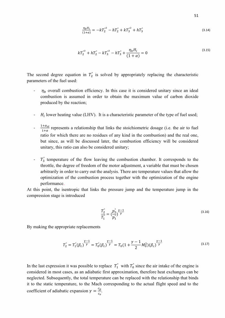
51

𝜂𝑏𝐻𝑖

(1+𝛼)= −𝑘𝑇2

°2− ℎ𝑇2

° + 𝑘𝑇3°2

+ ℎ𝑇3°

𝑘𝑇2°2

+ ℎ𝑇2° − 𝑘𝑇3

°2− ℎ𝑇3

° +𝜂𝑏𝐻𝑖

(1 + 𝛼)= 0

The second degree equation in 𝑇2° is solved by appropriately replacing the characteristic

parameters of the fuel used:

- 𝜂𝑏 overall combustion efficiency. In this case it is considered unitary since an ideal

combustion is assumed in order to obtain the maximum value of carbon dioxide

produced by the reaction;

- 𝐻𝑖 lower heating value (LHV). It is a characteristic parameter of the type of fuel used;

- 1+𝛼𝑠𝑡

1+𝛼 represents a relationship that links the stoichiometric dosage (i.e. the air to fuel

ratio for which there are no residues of any kind in the combustion) and the real one,

but since, as will be discussed later, the combustion efficiency will be considered

unitary, this ratio can also be considered unitary;

- 𝑇3° temperature of the flow leaving the combustion chamber. It corresponds to the

throttle, the degree of freedom of the motor adjustment, a variable that must be chosen

arbitrarily in order to carry out the analysis. There are temperature values that allow the

optimization of the combustion process together with the optimization of the engine

performance.

At this point, the isentropic that links the pressure jump and the temperature jump in the

compression stage is introduced

𝑇2°

𝑇1°

= (𝑝2

°

𝑝1°)

𝛾−1𝛾

By making the appropriate replacements

𝑇2° = 𝑇1

°(𝛽𝑐)𝛾−1

𝛾 = 𝑇0°(𝛽𝑐)

𝛾−1𝛾 = 𝑇0(1 +

𝛾 − 1

2𝑀0

2)(𝛽𝑐)𝛾−1

𝛾

In the last expression it was possible to replace 𝑇1° with 𝑇0

° since the air intake of the engine is

considered in most cases, as an adiabatic first approximation, therefore heat exchanges can be

neglected. Subsequently, the total temperature can be replaced with the relationship that binds

it to the static temperature, to the Mach corresponding to the actual flight speed and to the

coefficient of adiabatic expansion 𝛾 =𝑐𝑝

𝑐𝑣.

(3.16)

(3.14)

(3.15)

(3.17)

52

As for the second unknown 𝑝2° , it can be obtained as the product of significant pressure ratios,

station by station:

𝑝2° =

𝑝2°

𝑝1°

𝑝1°

𝑝0°

𝑝0°

𝑝0𝑝0

That is in other words

𝑝2° = 𝛽𝑐휀𝑑

𝑝0°

𝑝0𝑝0

Again, by exploiting the isentropic relations, the ratio between total and static pressure in

station 0 can be written, as

𝑝0°

𝑝0= (1 +

𝛾 − 1

2𝑀0

2)𝛾

𝛾−1

And replacing in the eq. 19

𝑝2° = 𝛽𝑐휀𝑑(1 +

𝛾 − 1

2𝑀0

2)𝛾

𝛾−1𝑝0

The pressure loss of the air intake is assumed unitary 휀𝑑 = 1, thus assuming an ideal efficiency

of the intake itself.

At this point we have found two expressions (eq. 3.21 and 3.17) that allow us to derive the two

unknown terms, 𝑇2° 𝑝2

° , which, when suitably substituted in the relations obtained by the

methods presented later, will allow an estimate of the pollutant emissions in on-design

conditions at pre-established altitude and flight conditions.

The only data required to carry out the analysis consist of:

- Dilution ratio of fuels in stoichiometric and non-stoichiometric conditions. Typically

the value of 𝑓 = 1 𝛼⁄ is around 0.0331. Nonetheless as anticipated, ratio 1+𝛼𝑠𝑡

1+𝛼 will be

considered unitary assuming an ideal combustion;

- Characteristics of the fuel, specifically lower heating value (𝐻𝑖);

- Ambient condition (𝑇0, 𝑝0) flight speed (𝑀0);

- Compression ratio (𝛽𝑐);

31 D. A. Sullivan, P. A. Mas, A Critical Review of NOx Correlations for Gas Turbine Combustors, in American Society of Mechanical Engineers, pp 3, 1976

(3.18)

(3.19)

(3.20)

(3.21)

53

In order to reduce the number of unknown variables required by the model presented, equation

17 and equation 15 are used by making a substitution. Assuming a temperature 𝑇3° at the end of

combustion (corresponding with the engine adjustment lever) it is possible to obtain the

compression ratio 𝛽𝑐.

𝑘[𝑇0(1 +𝛾−1

2𝑀0

2)(𝛽𝑐)𝛾−1

𝛾 ]2 + ℎ𝑇0(1 +𝛾−1

2𝑀0

2)(𝛽𝑐)𝛾−1

𝛾 − 𝑘𝑇3°2

− ℎ𝑇3° +

𝜂𝑏𝐻𝑖

(1+𝛼)= 0

𝑘𝑇02(1 +

𝛾−1

2𝑀0

2)2[(𝛽𝑐)𝛾−1

𝛾 ]2 + ℎ𝑇0(1 +𝛾−1

2𝑀0

2)(𝛽𝑐)𝛾−1

𝛾 − 𝑘𝑇3°2

− ℎ𝑇3° +

𝜂𝑏𝐻𝑖

(1+𝛼)= 0

From the previous one, solved as a second degree equation in (𝛽𝑐)𝛾−1

𝛾 it is possible to obtain

the value of 𝛽𝑐, which appropriately replaced in eq. 3.17 and 3.21, will allow to calculate the

two main variables unknowns, 𝑝2° and 𝑇2

°. The steps suggested above ensure the dependence of

the calculation on the fuel characteristics. In fact, the use of a different lower heating value will

allow the analysis of emissions to be carried out as a result of the choice of traditional fuels or

alternative fuels (biofuels).

In order to apply the method in its entirety, as is evident, knowledge of some parameters that

are not easy to hypothesize or to know a priori is required. References have been searched in

the literature which allow these variables to be approximated to experimentally obtained

average values in relation to other performance characteristics. For example, in the graph

below32 it is possible to establish a dependence between flight speed and the ratio between

thrust and air mass.

Figure 3.2 Thrust characteristics of typical aircraft engine

32 Jack D. Mattingly, Elements of gas turbine propulsion, 6 ed, New Delhi, Tata McGraw Hill, 2013, pp 28

(3.22)

(3.23)

54

In the hypothesis of obtaining the emission indexs for a standard LTO cycle, the flight speed

and consequently the speed of the flow entering the exoreactor can be obtained by consulting

this graph, after obtaining thrust and air flow values.

Instead, to obtain the mass of air, an approximation is made. According to Hill et al. , the dosage

(ratio between fuel flow and air flow into the engine) is typically equal 0.05. Knowing at this

point alpha and the fuel flow, which is also obtained from the ICAO prescriptions that describe

the standard cycle, it is possible to obtain the air flow.

Once these values have been obtained, the graph presented above can be exploited to derive the

maximum speed to be replaced in M0 for the calculation of emissions in each phase.

For the purposes of the calculation, knowledge of the fuel flow in the various phases of the LTO

cycle is required. As in the previous chapter, this information is set as input parameters. Or

alternatively knowledge of the SFC is required:

𝑤�̇� = 𝑆𝐹𝐶 ∙ 𝑇

𝑆𝐹𝐶 = 25𝑒(−0.05 𝐵𝑃𝑅) [𝑚𝑔/(𝑁 𝑠)]

Remembering that in the 4 distinct phases the thrust is equivalent to a fraction of the nominal

(100% take-off, 85% climb-out, 30% approach, 0.07% idle).

(3.24)

(3.25)

55

3.2 Emission calculation with correlation based models

The methods used for the emissions calculation all have a direct dependence on the two

parameters just calculated, 𝑝2° e 𝑇2

°, and have been drawn from previous and different studies.

They are called correlation based models

3.2.1 Nitrogen Oxides

For the calculation of nitrogen oxide emissions 𝑁𝑂𝑥33, the method proposed by AECMA34 -

European Association of Aerospace Industries- is used:

𝐸𝐼𝑁𝑂𝑋 = 2 + 28.5√𝑝2

°

3100exp (

𝑇2° − 825

250)

Alternatively, it is possible to calculate the emissions of nitrogen oxides using the method

proposed by NASA35.

𝐸𝐼𝑁𝑂𝑥 = 33.2(𝑝2

°

432.7)0.4exp (

𝑇2° − 459.67 − 1027

349.9+

6.29 − 6.3

53.2)

𝑝2° = Pressure of compressor exit (psia)

𝑇2°= Temperature of compressor exit (Deg R)

The NASA NEPP36 code used an equation to predict the NOx emissions at any given power

setting, based on the engine’s T3 and P3 conditions. The NASA NEPP data is not intended to

replicate any particular engine.

33 N. Chandrasekaran, A. Gua, Study of Prediction Methods for NOx Emission from Turbofan Engines, in Journal of Propulsion and Power, v. 28, n. 1, pp 179, Feb. 2012 34 Green, J. E., Greener by Design: The Technology Challenge, Aeronautical Journal, v. 106, n. 1056, pp. 57–113 Feb. 2002 35 David L. Daggett, Water Misting and Injection of Commercial Aircraft Engines to Reduce Airport Nox, pp 4, Seattle, Washington, National Aeronautics and Space Administration, 2004 36 The NEPP Program generates technical knowledge and recommendations about electrical, electronic, electromechanical (EEE) part performance, application, failure modes, test methods, reliability and supply chain quality within the context of NASA space flight missions and hardware. This information is made available to the NASA and high-reliability aerospace community through publications, web pages and links published on the website

(3.26)

(3.27)

56

3.2.2 Carbon dioxide and water

The carbon dioxide emissions 𝐶𝑂2 are calculated following the routine of the COPERT37

method (presented previously). In summary, this method exploits the combustion and molecular

characteristics, therefore it is independent from the performance of the propulsion system if not

for the dependence on the fuel flow rate.

Furthermore, to obtain the estimate of the maximum production of carbon dioxide, a unitary

combustion efficiency is assumed 𝜂𝑏 = 1, as anticipated in the discussion.

𝐸𝐶𝑂2,𝑡,𝑘𝐶𝐴𝐿𝐶 = 44.011


12.011 + 1.008 𝑟𝐻:𝐶,𝑡 + 16 𝑟𝑂:𝐶,𝑡

Alternatively, since carbon dioxide and water are the main products of hydrocarbon

combustion, their quantity emitted is directly proportional to the mass of fuel burned. In the

hypothesis of using an A-1 jet fuel, characterized by the molecular formula C12H23, 3156g of

CO2 and 1237g of H2O are produced for 1 kg of fuel. At this point it would be enough to have

the amount of fuel used. However, this method is valid only and exclusively for the calculation

of emissions deriving from the use of traditional fuels, thus not allowing a differentiated

treatment for biofuels. For this reason it is preferable to first use the COPERT method

(universal), and at the same time the calculation of water vapor will be subtracted from the

analysis.

3.2.3 Carbon monoxide

CO is formed by incomplete combustion and/or dissociation of CO2. Concentrations are high

at idle because of inadequate mixing, low temperature and fuel quenching on the walls38. The

CO carbon monoxide emissions are obtained from the relationship discussed by Deidewig et

al.39. Specifically, the emission index of carbon monoxide is related to the total volume of the

combustor 𝑉𝑐 and to the combustor loading parameter 𝜃𝑐:

𝐸𝐼𝐶𝑂 = 𝑓(𝑉𝑐 , 𝜃𝑐)

con 𝑉𝑐 combustor chamber volume, and

𝜃𝑐 = 𝑝2

° 𝑛 𝑒

𝑇2°

𝑏

𝑤𝑎𝑖𝑟

37 A. Bernetti, R. De Lauretis, G. Iarocci, F. Lena, R. Marra Campanale, E. Taurino, Inventario nazionale delle emissioni e disaggregazione provinciale, Istituto Superiore per la Ricerca e Protezione Ambientale, 2010 38 F. W. Lipfert, Correlation of Gas Turbine Emissions Data, in American Society of Mechanical Engineers, pp 3, 1972 39 F. Deidewig, A. Dopelheuer, M. Lecht, Methods to assess aircraft engine emissions in flight, ICAS-96-4.1.2, pp 136, DLR, Institute for Propulsion Technology, Cologne, Germany, 1996

(3.29)

(3.30)

(3.28)

57

where 𝑛 ≅ 1.75 and 𝑏 ≅ 300 𝐾

Ad esempio, per il caso particolare del CF6-50C2 (che verrà riportato in seguito), l’eq. 4.27 si

traduce in:

𝐸𝐼𝐶𝑂 = 369.6 (1

𝜃𝑐)2 − 14.96

1

𝜃𝑐+ 0.647

The German Aerospace Center (DLR) uses this alternative method. Emissions of CO and HC

result from incomplete combustion and are mostly produced at low power settings of the

engines, where the efficiency of the combustion process is low.40

This equation is obtained by Lefebvre correlation, that contains many common variables that

effect CO levels include combustor inlet pressure, pressure drop, primary zone temperature

(Tpz) and a ratio between the volume of combustion (Vc) and the volume needed for fuel to

evaporate (Ve)41.

𝐸𝐼𝐶𝑂 =86 ∙ 𝑚𝑎̇ ∙ 𝑇𝑝𝑧 ∙ exp (−0.0035𝑇𝑝𝑧)

(𝑉𝑐−𝑉𝑒)√∆𝑝2𝑝2

𝑝31.5

3.2.4 Hydrocarbons

The combustion residues, which occur when the combustion efficiency is not uniform, are

mainly made up of CO and HC42. Specifically, unburnt HC hydrocarbons represent on average

about 1% of total CO2 and H2O emissions. Their production is closely linked, as anticipated,

to the efficiency of the combustion process 𝜂𝑐

𝜂𝑐 = 100 − 0.1 ∙ 𝐸𝐼𝐻𝐶 − 0.02334 ∙ 𝐸𝐼𝐶𝑂 [%]

This formulation, proposed by the German Aerospace Center (DLR) uses an alternative

method, and is valid if the combustion efficiency is known a priori. In the case under

40 Martin Shaefer, Methodologies for Aviation Emission Calculation – A comparison of alternative approaches towards 4D global inventories, Berlin University of Technology, 2006 41 Michael David Marchand, Multi-Dimensional Carbon Monoxide Emissions Predictor for Preliminary Gas Turbine Combustor Design Optimization, University of Toronto, 2013 42 C.J. Eyers, D. Addleton, K. Atkinson, M.J. Broomhead, R. Christou, T. Elliff, R. Falk, I. Gee, D.S. Lee, C. Marizy, S. Michot, J. Middel, P. Newton, P. Norman, D. Raper, N. Stanciou, AERO2K Global Aviation Emissions Inventories for 2002 and 2025, Tech. Rep. QinetiQ, Farnbourugh, UK, 2004

(3.31)

(3.33)

(3.32)

58

consideration, however, there is no information regarding the process, in fact for the calculation

of carbon dioxide emissions the efficiency is assumed to be unitary (which would exclude the

generation of unburnt substances). Consequently, we are limited to calculating the hydrocarbon

emissions as a fraction of the total amount of carbon dioxide and water emissions, and being an

entity less than 0.01%, the calculation of the EIHC will be neglected.

3.3 Example of calculation

Below is an example of calculating the emissions on the LTO cycle of the CF6-50C2, a 230.5

kN nominal thrust engine. According to the ICAO requirements for the LTO cycle, the fuel

flow for each phase is:

- T/O 2.36 kg/s

- C/O 1.94 kg/s

- App 0.668 kg/s

- Idle 0.163 kg/s

The main performance characteristics of the turbofan under consideration are summarized

below.

Figure 3.3 Specifications for General Electric CF6-50C243

As evident in the analysis carried out previously, knowledge of the end-of-combustion

temperature TET, 𝑇3° is of fundamental importance. In this case the maximum value is equal to

1650 ° K. This temperature affects the dosage f, the ratio between fuel flow and air flow. In

static conditions at sea level, the fuel flow rate will be equal to the product of SFC and thrust:

43 Elodie Roux, Turbofan and Turbojet Engines Database Handbook, Edition Elodie Roux, Blagnac, France, 2007

59

𝑤�̇� = 𝑆𝐹𝐶 ∙ 𝑇 = 230500 ∙ 1.05 ∙ 10−5 = 2.42 𝑘𝑔/𝑠

This value is obtained using the maximum thrust value, for the purpose of analyzing the LTO

cycle, and corresponds to the takeoff conditions; it will therefore be necessary to jointly

evaluate the fuel flow rate in relation to the reduced thrust values for climb out, approach and

taxi.

𝑤𝑓,𝐶𝑂̇ = 𝑆𝐹𝐶 ∙ 𝑇 ∙ 0.85 = 195925 ∙ 1.05 ∙ 10−5 = 2.057 𝑘𝑔/𝑠

𝑤𝑓,𝐴𝑝𝑝̇ = 𝑆𝐹𝐶 ∙ 𝑇 ∙ 0.3 = 69150 ∙ 1.05 ∙ 10−5 = 0.7260 𝑘𝑔/𝑠

𝑤𝑓,𝐼𝑑𝑙𝑒̇ = 𝑆𝐹𝐶 ∙ 𝑇 ∙ 0.07 = 16135 ∙ 1.05 ∙ 10−5 = 0.1694 𝑘𝑔/𝑠

The values just calculated differ slightly from those provided within the ICAO database.

Another parameter to be obtained in order to complete the performance analysis and

consequently the emissions is the speed of the flow entering the engine, 𝑀0. For this purpose

the graph presented previously is exploited (Figure 3.2). From the data obtained in the literature,

the end-of-combustion temperature in the specific engine considered varies between a

minimum of 1450 ° K and 1663 ° K44. By making an approximation and assuming that the trend

between the thrust generated and the TIT is linear and linked by direct proportionality, the value

of 𝑇3can be obtained for each phase of the LTO cycle. Consequently, through the graph of the

following figure (3.4), it is possible to obtain the dosage ratio corresponding to each turbine

inlet temperature, assuming that the temperature of the reagents is 400 ° K.

44 C56–50A Engines, Aircraft Engineering and Aerospace Technology, Vol. 43 No. 9, pp. 28-32, 1971

(3.34)

(3.35)

(3.36)

(3.37)

60

Figure 3.4 Trend of the dosage f as a function of the end-of-combustion temperature45

At this point, all the data necessary to carry out the analysis are available. The table shows the

input data (marked by blue) and the simulation results (in red).

Table 3.1 Data and results of simulation for CF6-50C2 using Jet-A1

Take Off Climb Out Approach Idle

Thrust [N] 230500 195925 69150 16135

T3 [K] 1663 1631.5 1513.9 1464.9

f 0.037 0.036 0.0335 0.033

Fuel Flow [kg/s] 2.42 2.057 0.726 0.1694

M0 0.05 0.23 0.5 0.3

T2 [K] 462.658 458.175 399.323 355.7437

p2 [bar] 4.616 4.464 2.757 1.84

Beta c 4.494 3.799 2.617 1.855

EICO [g/kg] 0.75 0.45 22.959 20.778

EICO2 [kg] 8.557 7.034 2.422 0.591

EINOx [g/kg] 24.284 23.407 14.265 9.7

EIHC [g/kg] 0.536 0.553 0.457 0.705

The trends in CO and HC emissions are in contrast with those of CO2 and NOx: while the

former decrease as 𝑇2, 𝑇3 and fuel flow increase, the latter are characterized by proportional

growth.

45 P. G. Hill, C. R. Peterson, Mechanics and thermodynamics of propulsion, pp 244, Addison-Wesley Publishing Company, Cambridge,1992

61

The data thus obtained, as anticipated at the beginning of the chapter, refer to an LTO cycle for

the certification and control of pollutants, and will be the starting point for the application of

the Fuel Flow Method 2 of chapter 2.

Figure 3.5 Emissions index related to F.F. for CO, CO2, HC and Nox for JET-A1

Figure 3.6 Emissions index related to T2 for CO, CO2, HC and Nox for JET-A1

62

The advantage, in addition to the possibility of inserting exoreactors in the database for which

there are no experimental data, lies in the fact of being able to carry out analyzes also for

performances deriving from the use of unconventional fuels, thanks to the dependence of the

calculation of temperatures and pressures in the combustor by the characteristics of the fuel

itself, and specifically its efficiency and its lower calorific value.

Below is the analysis of the performance of the same engine, in the event that it is powered by

a mixture made up of 100% CSPK

As known, LHV becomes an utmost factor that influence engine thrust. Besides LHV, heat

capacity of the combustible mixture (fuel and air) (Cp) could be another factor that might affect

the amount of thrust generated by an aircraft engine. By the way, the LHV of JSPK is higher

than that of CSPK (JSPK = 44.3 MJ/kg and CSPK = 44.0 MJ/kg)46.

Again, the data used and the results obtained are presented in the table below.

Table 3.2 Data and results of simulation for CF6-50C2 using CSPK

Take Off Climb Out Approach Idle

Thrust [N] 230500 195925 69150 16135

T3 [K] 1663 1631.5 1513.9 1464.9

f 0.037 0.036 0.0335 0.033

Fuel Flow [kg/s] 2.36 1.94 0.668 0.163

M0 0.23 0.5 0.3 0.05

T2 [K] 443.713 439.705 381.857 338.351

p2 [bar] 3.987 3.863 2.357 1.544

Beta c 4.494 3.799 2.617 1.855

EICO [g/kg] 16.374 13.865 77.31 72.67

EICO2 [kg] 8.557 7.034 2.422 0.591

EINOx [g/kg] 20.775 20.094 12.248 8.2665

EIHC [g/kg] 0.4498 0.4803 0.4763 0.6178

46 Effects of biofuels properties on aircraft engine performance, in Aircraft Engineering and aerospace technology, 87(5), pp 437-443, Emerald, 2013

63

Figure 3.7 Emissions index related to F.F. for CO, CO2, HC and Nox for CSPK

Figure 3.8 Emissions index related to T2 for CO, CO2, HC and Nox for CSPK

64

Conclusions

From the results obtained, it is possible to deduce that the application of biofuels, as anticipated

by previous studies, is not so advantageous from the point of view of the reductions in emissions

produced during an operating cycle as a consequence of the combustion process.

The different lower heating value, which varies from fuel to fuel, and the different molecular

structure affect the process inside the combustion chamber, causing the variation of

fundamental parameters of pressure, temperature and dosage ratio between the amount of air

and fuel burne.

In fact, some of the pollutants, such as nitrogen oxides, are emitted in larger quantities if we

compare the use of biofuels to the use of A1 jet fuel. The other compounds, and specifically the

carbon monoxides, on the other hand, have an opposite trend, decreasing both in the case of

CSPK and JSPK. The latter are calculated only if the combustion process is not considered

ideal. Otherwise, an estimation of carbon dioxide emissions can be made, which according to

the estimates made is reduced, albeit to a negligible extent, due to the effect of the application

of alternative fuels. For this last occurrence, it should be specified that the advantage in the use

of biofuels does not lie so much in the analysis of the operating cycle and combustion, but if

we refer to the well to wheel life cycle, they certainly offer a valid application in order to reduce

the environmental impact of air transport. In fact, being fuels obtained from biomass, they

guarantee a limitation of carbon emissions deriving from the characteristic extraction and

production processes of kerosene. They are therefore considered potential substitutes for the

power supply of aeronautical engines, both for the environmental advantages and for their

potential application regardless of the changes to be made to the configuration of pre-existing

aircraft.

65

Appendix A

Matlab code for Fuel Flow method application

%% LETTURA DATI DA DATABASE

clear all

clc

disp('LETTURA DATI DA DATABASE');

spinta_tot=input('inserisci valore di spinta compreso tra 40 e 500

kN:');

numero_motori=input('inserisci numero motori (2 o 4):');

carburante1=input('Inserire 1 per JET-A, 2 per CSPK, 3 per JSPK:');

spinta=spinta_tot/numero_motori;

% CASO JET-A

if carburante1==1

[JETA,

MOTORE]=xlsread('DATABASE\DATABASE_JETA.xlsx','A2:AF620');

i=0;

for i=1:619

if spinta==JETA(i,1) || (spinta>JETA(i,1) &&

spinta<JETA(i+1,1))

mot=MOTORE(i, 1:2)

EIHC_TO=JETA(i,2);

EIHC_CO=JETA(i,3);

EIHC_App=JETA(i,4);

EIHC_Idle=JETA(i,5);

EICO2_TO=JETA(i,7);

EICO2_CO=JETA(i,8);

EICO2_App=JETA(i,9);

EICO2_Idle=JETA(i,10);

EICO_TO=JETA(i,11);

EICO_CO=JETA(i,12);

EICO_App=JETA(i,13);

EICO_Idle=JETA(i,14);

EINOx_TO=JETA(i,16);

EINOx_CO=JETA(i,17);

EINOx_App=JETA(i,18);

EINOx_Idle=JETA(i,19);

WF_SL_TO=JETA(i,21);

WF_SL_CO=JETA(i,22);

WF_SL_App=JETA(i,23);

WF_SL_Idle=JETA(i,24);

else

i=i+1;

end

end

%CASO CSPK

elseif carburante1==2

blend=input('Inserire percentuale miscela (20, 40, 60, 80,

100):');

if blend==20

[CSPK20,

MOTORE]=xlsread('DATABASE\DATABASE_CSPK20.xlsx','A2:AR620');

i=0;

for i=1:619

66

if spinta==CSPK20(i,1) ||

(spinta>CSPK20(i,1) && spinta<CSPK20(i+1,1))

mot=MOTORE(i, 1:2)

EIHC_TO=CSPK20(i,2);

EIHC_CO=CSPK20(i,3);

EIHC_App=CSPK20(i,4);

EIHC_Idle=CSPK20(i,5);

EICO2_TO=CSPK20(i,7);

EICO2_CO=CSPK20(i,8);

EICO2_App=CSPK20(i,9);

EICO2_Idle=CSPK20(i,10);

EICO_TO=CSPK20(i,11);

EICO_CO=CSPK20(i,13);

EICO_App=CSPK20(i,15);

EICO_Idle=CSPK20(i,17);

EINOx_TO=CSPK20(i,20);

EINOx_CO=CSPK20(i,22);

EINOx_App=CSPK20(i,24);

EINOx_Idle=CSPK20(i,26);

WF_SL_TO=CSPK20(i,29);

WF_SL_CO=CSPK20(i,31);

WF_SL_App=CSPK20(i,33);

WF_SL_Idle=CSPK20(i,35);

else

i=i+1;

end

end

elseif blend==40

[CSPK40,


i=0;

for i=1:619



mot=MOTORE(i, 1:2)





















else

67

i=i+1;

end

end

elseif blend==60

[CSPK60,


i=0;

for i=1:619



mot=MOTORE(i, 1:2)





















else

i=i+1;

end

end

elseif blend==80

[CSPK80,


i=0;

for i=1:619



mot=MOTORE(i, 1:2)













68









else

i=i+1;

end

end

elseif blend==100

[CSPK100,


i=0;

for i=1:619



mot=MOTORE(i, 1:2)





















else

i=i+1;

end

end

end

%CASO JSPK

elseif carburante1==3

blend=input('Inserire percentuale miscela (20, 40, 60, 80,

100):');

if blend==20

[JSPK20,

MOTORE]=xlsread('DATABASE\DATABASE_JSPK20.xlsx','A2:AR620');

i=0;

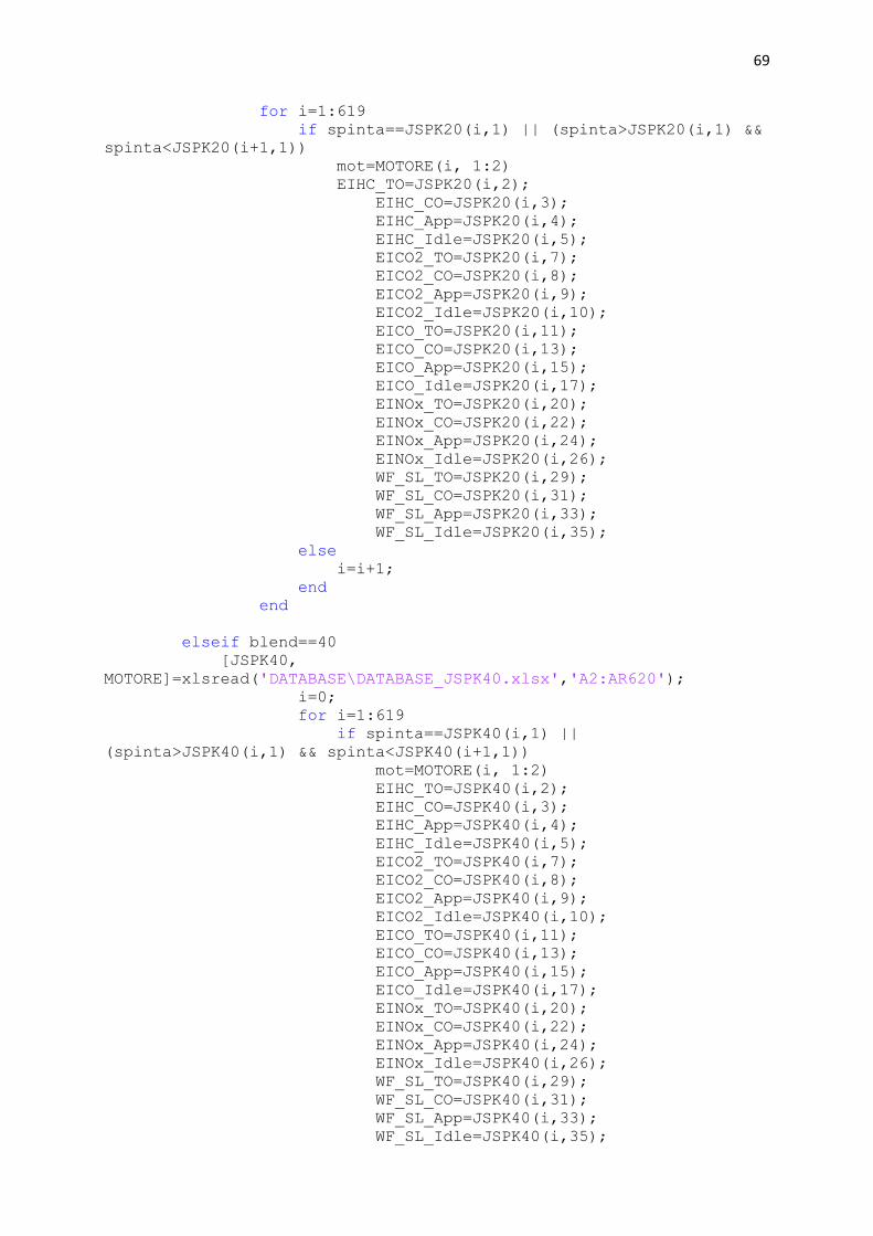
69

for i=1:619

if spinta==JSPK20(i,1) || (spinta>JSPK20(i,1) &&

spinta<JSPK20(i+1,1))

mot=MOTORE(i, 1:2)

EIHC_TO=JSPK20(i,2);

EIHC_CO=JSPK20(i,3);

EIHC_App=JSPK20(i,4);

EIHC_Idle=JSPK20(i,5);

EICO2_TO=JSPK20(i,7);

EICO2_CO=JSPK20(i,8);

EICO2_App=JSPK20(i,9);

EICO2_Idle=JSPK20(i,10);

EICO_TO=JSPK20(i,11);

EICO_CO=JSPK20(i,13);

EICO_App=JSPK20(i,15);

EICO_Idle=JSPK20(i,17);

EINOx_TO=JSPK20(i,20);

EINOx_CO=JSPK20(i,22);

EINOx_App=JSPK20(i,24);

EINOx_Idle=JSPK20(i,26);

WF_SL_TO=JSPK20(i,29);

WF_SL_CO=JSPK20(i,31);

WF_SL_App=JSPK20(i,33);

WF_SL_Idle=JSPK20(i,35);

else

i=i+1;

end

end

elseif blend==40

[JSPK40,


i=0;

for i=1:619

if spinta==JSPK40(i,1) ||

(spinta>JSPK40(i,1) && spinta<JSPK40(i+1,1))

mot=MOTORE(i, 1:2)





















70

else

i=i+1;

end

end

elseif blend==60

[JSPK60,


i=0;

for i=1:619



mot=MOTORE(i, 1:2)





















else

i=i+1;

end

end

elseif blend==80

[JSPK80,


i=0;

for i=1:619



mot=MOTORE(i, 1:2)












71










else

i=i+1;

end

end

elseif blend==100

[JSPK100,MOTORE]=xlsread('DATABASE\DATABASE_JSPK100.xlsx','A2:AR620'

);

i=0;

for i=1:619



mot=MOTORE(i, 1:2)





















else

i=i+1;

end

end

end

end

WF_SL=[WF_SL_TO WF_SL_CO WF_SL_App WF_SL_Idle];

EICO2_SL=[EICO2_TO EICO2_CO EICO2_App EICO2_Idle];

EICO_SL=[EICO_TO EICO_CO EICO_App EICO_Idle];

EIHC_SL=[EIHC_TO EIHC_CO EIHC_App EIHC_Idle];

EINOx_SL=[EINOx_TO EINOx_CO EINOx_App EINOx_Idle];

72

figure

loglog(WF_SL, EICO_SL , '- r *', WF_SL, EICO2_SL, '- y *', WF_SL,

EIHC_SL, '- b *', WF_SL, EINOx_SL, '- g *')

grid on;

xlabel("Portata combustibile S.L");

ylabel("Emissioni [g/kg]");

title("Andamento emissioni");

legend("CO_s_l", "CO2_s_l", "HC_s_l", "NOx_s_l");

%% CALCOLO EMISSIONI LTO CYCLE

%emissioni_tot_hc_idle= WF_SL_Idle*EIHC_Idle*1560;

%emissioni_tot_hc_to= WF_SL_TO*EIHC_TO*42;

%emissioni_tot_hc_co= WF_SL_CO*EIHC_CO*132;

%emissioni_tot_hc_app= WF_SL_App*EIHC_App*240;

%emissioni_tot_co_idle= WF_SL_Idle*EICO_Idle*1560;

%emissioni_tot_co_to= WF_SL_TO*EICO_TO*42;

%emissioni_tot_co_co= WF_SL_CO*EICO_CO*132;

%emissioni_tot_co_app= WF_SL_App*EICO_App*240;

%emissioni_tot_co2_idle= WF_SL_Idle*EICO2_Idle*1560;

%emissioni_tot_co2_to= WF_SL_TO*EICO2_TO*42;

%emissioni_tot_co2_co= WF_SL_CO*EICO2_CO*132;

%emissioni_tot_co2_app= WF_SL_App*EICO2_App*240;

%emissioni_tot_nox_idle= WF_SL_Idle*EINOx_Idle*1560;

%emissioni_tot_nox_to= WF_SL_TO*EINOx_TO*42;

%emissioni_tot_nox_co= WF_SL_CO*EINOx_CO*132;

%emissioni_tot_nox_app= WF_SL_App*EINOx_App*240;

WF_SL=[0 numero_motori*WF_SL_TO numero_motori*WF_SL_CO

numero_motori*WF_SL_App numero_motori*WF_SL_Idle];

EICO2_SL=[0 numero_motori*EICO2_TO numero_motori*EICO2_CO

numero_motori*EICO2_App numero_motori*EICO2_Idle];

EICO_SL=[0 numero_motori*EICO_TO numero_motori*EICO_CO

numero_motori*EICO_App numero_motori*EICO_Idle];

EIHC_SL=[0 numero_motori*EIHC_TO numero_motori*EIHC_CO

numero_motori*EIHC_App numero_motori*EIHC_Idle];

EINOx_SL=[0 numero_motori*EINOx_TO numero_motori*EINOx_CO

numero_motori*EINOx_App numero_motori*EINOx_Idle];

vett_t=[0 1560 1560 1602 1602 1734 1734 1974];

vett_em_CO=[EICO_SL(2) EICO_SL(2) EICO_SL(3) EICO_SL(3) EICO_SL(4)

EICO_SL(4) EICO_SL(5) EICO_SL(5)];

vett_em_HC=[EIHC_SL(2) EIHC_SL(2) EIHC_SL(3) EIHC_SL(3) EIHC_SL(4)

EIHC_SL(4) EICO_SL(5) EICO_SL(5)];

vett_em_NOx=[EINOx_SL(2) EINOx_SL(2) EINOx_SL(3) EINOx_SL(3)

EINOx_SL(4) EINOx_SL(4) EINOx_SL(5) EINOx_SL(5)];

vett_em_CO2=[EICO2_SL(2) EICO2_SL(2) EICO2_SL(3) EICO2_SL(3)

EICO2_SL(4) EICO2_SL(4) EICO2_SL(5) EICO2_SL(5)];

figure

plot(vett_t,vett_em_CO, '- r *','LineWidth',3);

title("EI CO LTO CYCLE");

xlabel("Time [s]");

73

ylabel("EI [g/kg]");

grid on

figure

plot(vett_t,vett_em_HC, '- r *','LineWidth',3);

title("EI HC LTO CYCLE");

xlabel("Time [s]");


grid on

figure

plot(vett_t,vett_em_CO2, '- r *','LineWidth',3);

title("EI CO2 LTO CYCLE");

xlabel("Time [s]");


grid on

figure

plot(vett_t,vett_em_NOx, '- r *','LineWidth',3);

title("EI NOx LTO CYCLE");

xlabel("Time [s]");


grid on

%% CALCOLO EMISSIONI AL VARIARE DELLA QUOTA / FUEL FLOW METHOD

disp('CALCOLO EMISSIONI AL VARIARE DELLA QUOTA / FUEL FLOW METHOD');

disp('INSERIMENTO CARATTERISTICHE MISSION PROFILE');

M_idle = input ('Inserire MACH massimo di taxi :');

M_TO = input('inserire MACH massimo di takeoff :');

M_CO = input('inserire MACH massimo di climbout :');

M_cruise = input('inserire MACH massimo di cruise :');

M_app = input('inserire MACH massimo di approach :');

M_landing = input('Inserire MACH massimo atterraggio :');

t_idle=input('Inserire durata manovra di taxi [s]:');

t_TO=input('Inserire durata manovra di decollo [s]:');

t_CO=input('Inserire durata totale climb out [s]:');

t_cruise=input('inserire durata totale crociera [s]:');

t_app=input('Inserire durata totale manovra avvicinamento [s]:');

t_landing=input('Inserire durata totale atterraggio [s]:');

z0_idle= input('inserire quota di decollo: ');

zf_idle= z0_idle;

z0_TO= z0_idle;

zf_TO= input('inserire quota fine manovra decollo: ');

z0_CO= zf_TO;

zf_CO= input('inserire quota fine climb out: ');

z0_cruise=zf_CO;

zf_cruise=z0_cruise;

z0_app= zf_CO;

zf_app= input('inserire quota di fine approach: ');

z0_landing=zf_app;

zf_landing=z0_landing;

74

Consumo_idle=input('Inserire portata combustibile della manovra di

taxi:');

Consumo_TO=input('Inserire portata combustibile della manovra di

decollo:');

Consumo_CO=input('Inserire portata combustibile della manovra di

climb-out:');

Consumo_cruise=input('Inserire portata combustibile in crociera:');

Consumo_app=input('Inserire portata combustibile della manovra di

avvicinamento:');

Consumo_landing=input('Inserire portata combustibile di

atterraggio:');

% PLOT DEL MISSION PROFILE

t_vett=[0 t_idle t_idle+t_TO t_idle+t_TO+t_CO

t_idle+t_TO+t_CO+t_cruise t_idle+t_TO+t_CO+t_cruise+t_app

t_idle+t_TO+t_CO+t_cruise+t_app+t_landing];

z_vett=[0 0 zf_TO zf_CO zf_CO zf_app 0];

figure

plot(t_vett,z_vett);

dt=1;

t_tot=t_idle+t_TO+t_CO+t_cruise+t_app+t_landing;

for t=1:t_tot

if t<t_idle

n=t_idle;

M=linspace(0,M_idle,n);

z=linspace(1,zf_idle,n);

T_amb=(15-0.0065.*z)+273.15;

p_amb=1.01325.*(T_amb./288.15).^5.25;

theta_amb=T_amb./518.67;

delta_amb=p_amb./14.696;

Consumo_idle_vet=linspace(0, Consumo_idle,n);

Wf_sl_idle=Consumo_idle_vet.*(theta_amb.^4.5)./(delta_amb).*exp(0.2.

*(M.^2));

F1=interp1(WF_SL, EICO2_SL, Wf_sl_idle, 'linear', 'extrap');

G1=interp1(WF_SL, EICO_SL, Wf_sl_idle, 'linear', 'extrap');

H1=interp1(WF_SL, EIHC_SL, Wf_sl_idle, 'linear', 'extrap');

I1=interp1(WF_SL, EINOx_SL, Wf_sl_idle, 'linear', 'extrap');

CO2_TOT_IDLE = F1.*((theta_amb.^3.3)./(delta_amb.^1.02));

CO_TOT_IDLE =

G1.*((theta_amb.^3.3)./(delta_amb.^1.02)).*Consumo_idle;%*(Consumo_i

dle*t_idle);%calcolo g di emissioni tramite fuel flow. Se non

effettuassi correzione, avrei g/kg come nel database

HC_TOT_IDLE =

H1.*((theta_amb.^3.3)./(delta_amb.^1.02)).*Consumo_idle;%*(Consumo_i

dle*t_idle);

NOx_TOT_IDLE =

I1.*(((delta_amb.^1.02)./(theta_amb.^3.3)).^0.5).*Consumo_idle;%*(Co

nsumo_idle*t_idle);

elseif (t>t_idle && t<(t_idle+t_TO))

n=t_TO;

75

M=linspace(M_idle, M_TO ,n);

z=linspace(zf_idle,zf_TO,n);

T_amb=(15-0.0065.*z)+273.15;

p_amb=1.01325.*(T_amb./288.15).^5.25;



Consumo_TO_vet=linspace(Consumo_idle, Consumo_TO,n);

Wf_sl_TO=Consumo_TO_vet.*(theta_amb.^4.5)./(delta_amb).*exp(0.2.*(M.

^2));

F2=interp1(WF_SL, EICO2_SL, Wf_sl_TO, 'linear', 'extrap');

G2=interp1(WF_SL, EICO_SL, Wf_sl_TO, 'linear', 'extrap');

H2=interp1(WF_SL, EIHC_SL, Wf_sl_TO, 'linear', 'extrap');

I2=interp1(WF_SL, EINOx_SL, Wf_sl_TO, 'linear', 'extrap');

CO2_TOT_TO = F2.*((theta_amb.^3.3)./(delta_amb.^1.02));

CO_TOT_TO =

G2.*((theta_amb.^3.3)./(delta_amb.^1.02)).*Consumo_TO;%*(Consumo_TO*

t_TO);

HC_TOT_TO =

H2.*((theta_amb.^3.3)./(delta_amb.^1.02)).*Consumo_TO;%*(Consumo_TO*

t_TO);

NOx_TOT_TO =

I2.*(((delta_amb.^1.02)./(theta_amb.^3.3)).^0.5).*Consumo_TO;%*(Cons

umo_TO*t_TO);

elseif (t>(t_idle+t_TO) && t<(t_idle+t_TO+t_CO))

n=t_CO;

M=linspace(M_TO, M_CO ,n);

z=linspace(zf_TO,zf_CO,n);

T_amb=(15-0.0065.*z)+273.15;

p_amb=1.01325.*(T_amb./288.15).^5.25;



Consumo_CO_vet=linspace(Consumo_TO, Consumo_CO, n);

Wf_sl_CO=Consumo_CO_vet.*(theta_amb.^4.5)./(delta_amb).*exp(0.2.*(M.

^2));

F3=interp1(WF_SL, EICO2_SL, Wf_sl_CO, 'linear', 'extrap');

G3=interp1(WF_SL, EICO_SL, Wf_sl_CO, 'linear', 'extrap');

H3=interp1(WF_SL, EIHC_SL, Wf_sl_CO, 'linear', 'extrap');

I3=interp1(WF_SL, EINOx_SL, Wf_sl_CO, 'linear', 'extrap');

CO2_TOT_CO = F3.*((theta_amb.^3.3)./(delta_amb.^1.02));

CO_TOT_CO =

G3.*((theta_amb.^3.3)./(delta_amb.^1.02)).*Consumo_CO;%*(Consumo_CO*

t_CO);

HC_TOT_CO =

H3.*((theta_amb.^3.3)./(delta_amb.^1.02)).*Consumo_CO;%*(Consumo_CO*

t_CO);

NOx_TOT_CO =

I3.*(((delta_amb.^1.02)./(theta_amb.^3.3)).^0.5).*Consumo_CO;%*(Cons

umo_CO*t_CO);

76

elseif (t>(t_idle+t_TO+t_CO) && t<(t_idle+t_TO+t_CO+t_cruise))

n=t_cruise;

M=(M_cruise*ones(n,1))';%linspace(M_CO,M_cruise,n);

z=(zf_cruise*ones(n,1))'; %linspace(zf_cruise,zf_cruise,n);

T_amb=(15-0.0065.*z)+273.15;

p_amb=1.01325.*(T_amb./288.15).^5.25;



Consumo_cruise_vet=

(Consumo_cruise*ones(n,1))';%linspace(Consumo_CO,Consumo_cruise, n);

Wf_sl_cruise=Consumo_cruise_vet.*(theta_amb.^4.5)./(delta_amb).*exp(

0.2.*(M.^2));

F4=interp1(WF_SL, EICO2_SL, Wf_sl_cruise, 'linear',

'extrap');

G4=interp1(WF_SL, EICO_SL, Wf_sl_cruise, 'linear',

'extrap');

H4=interp1(WF_SL, EIHC_SL, Wf_sl_cruise, 'linear',

'extrap');

I4=interp1(WF_SL, EINOx_SL, Wf_sl_cruise, 'linear',

'extrap');

CO2_TOT_CRUISE = F4.*((theta_amb.^3.3)./(delta_amb.^1.02));

CO_TOT_CRUISE =

G4.*((theta_amb.^3.3)./(delta_amb.^1.02)).*Consumo_cruise;%*(Consumo

_app*t_app);

HC_TOT_CRUISE =

H4.*((theta_amb.^3.3)./(delta_amb.^1.02)).*Consumo_cruise;%*(Consumo

_app*t_app);

NOx_TOT_CRUISE =

I4.*(((delta_amb.^1.02)./(theta_amb.^3.3)).^0.5).*Consumo_cruise;%*(

Consumo_app*t_app);

elseif (t>(t_idle+t_TO+t_CO+t_cruise) &&

t<(t_idle+t_TO+t_CO+t_cruise+t_app))

n=t_app;

M=linspace(M_cruise,M_app,n);

z=linspace(zf_CO,zf_app,n);

T_amb=(15-0.0065.*z)+273.15;

p_amb=1.01325.*(T_amb./288.15).^5.25;



Consumo_app_vet=linspace(Consumo_cruise,Consumo_app, n);

Wf_sl_app=Consumo_app_vet.*(theta_amb.^4.5)./(delta_amb).*exp(0.2.*(

M.^2));

F5=interp1(WF_SL, EICO2_SL, Wf_sl_app, 'linear', 'extrap');

G5=interp1(WF_SL, EICO_SL, Wf_sl_app, 'linear', 'extrap');

H5=interp1(WF_SL, EIHC_SL, Wf_sl_app, 'linear', 'extrap');

I5=interp1(WF_SL, EINOx_SL, Wf_sl_app, 'linear', 'extrap');

CO2_TOT_APP = F5.*((theta_amb.^3.3)./(delta_amb.^1.02));

CO_TOT_APP =

G5.*((theta_amb.^3.3)./(delta_amb.^1.02)).*Consumo_app;%*(Consumo_ap

p*t_app);

77

HC_TOT_APP =

H5.*((theta_amb.^3.3)./(delta_amb.^1.02)).*Consumo_app;%*(Consumo_ap

p*t_app);

NOx_TOT_APP =

I5.*(((delta_amb.^1.02)./(theta_amb.^3.3)).^0.5).*Consumo_app;%*(Con

sumo_app*t_app);

elseif (t>(t_idle+t_TO+t_CO+t_cruise+t_app) &&

t<(t_idle+t_TO+t_CO+t_cruise+t_app+t_landing))

n=t_landing;

M=linspace(M_landing,0,n);

z=linspace(zf_CO,zf_app,n);

T_amb=(15-0.0065.*z)+273.15;

p_amb=1.01325.*(T_amb./288.15).^5.25;



Consumo_landing_vet=linspace(Consumo_landing,0, n);

Wf_sl_landing=Consumo_landing_vet.*(theta_amb.^4.5)./(delta_amb).*ex

p(0.2.*(M.^2));

F6=interp1(WF_SL, EICO2_SL, Wf_sl_landing, 'linear',

'extrap');

G6=interp1(WF_SL, EICO_SL, Wf_sl_landing, 'linear',

'extrap');

H6=interp1(WF_SL, EIHC_SL, Wf_sl_landing, 'linear',

'extrap');

I6=interp1(WF_SL, EINOx_SL, Wf_sl_landing, 'linear',

'extrap');

CO2_TOT_LANDING = F6.*((theta_amb.^3.3)./(delta_amb.^1.02));

CO_TOT_LANDING =

G6.*((theta_amb.^3.3)./(delta_amb.^1.02)).*Consumo_landing;%*(Consum

o_app*t_app);

HC_TOT_LANDING =

H6.*((theta_amb.^3.3)./(delta_amb.^1.02)).*Consumo_landing;%*(Consum

o_app*t_app);

NOx_TOT_LANDING =

I6.*(((delta_amb.^1.02)./(theta_amb.^3.3)).^0.5).*Consumo_landing;%*

(Consumo_app*t_app);

end

t=t+dt;

end

%% PLOT CONSUMI SU MISSION PROFILE

figure

grid on

CO2_TOT=[CO2_TOT_IDLE CO2_TOT_TO CO2_TOT_CO CO2_TOT_CRUISE

CO2_TOT_APP CO2_TOT_LANDING];

m=length(CO2_TOT);

T=linspace(0,t_tot,m);

yyaxis left

78

plot(T, CO2_TOT, 'r');

title("ANDAMENTO EMISSIONI CO2 NEL TEMPO DI MISSIONE");

xlabel("Tempo [s]");

ylabel("Emissioni [kg]");

hold on

yyaxis right

plot(t_vett,z_vett, 'b', 'LineWidth',2);

ylabel("Quota [10^3 m]");

figure

grid on

CO_TOT=[CO_TOT_IDLE CO_TOT_TO CO_TOT_CO CO_TOT_CRUISE CO_TOT_APP

CO_TOT_LANDING];

yyaxis left

plot(T, CO_TOT, 'r');

title("ANDAMENTO EMISSIONI CO NEL TEMPO DI MISSIONE");



hold on

yyaxis right



figure

grid on

HC_TOT=[HC_TOT_IDLE HC_TOT_TO HC_TOT_CO HC_TOT_CRUISE HC_TOT_APP

HC_TOT_LANDING];

yyaxis left

plot(T, HC_TOT, 'r');

title("ANDAMENTO EMISSIONI HC NEL TEMPO DI MISSIONE");



hold on

yyaxis right



figure

grid on

NOx_TOT=[NOx_TOT_IDLE NOx_TOT_TO NOx_TOT_CO NOx_TOT_CRUISE

NOx_TOT_APP NOx_TOT_LANDING];

yyaxis left

plot(T, NOx_TOT, 'r');

title("ANDAMENTO EMISSIONI TO NEL TEMPO DI MISSIONE");



hold on

yyaxis right



%% PLOT ISTOGRAMMI CONSUMI

figure

K= [1 2 3 4 5 6];

CO= [ sum(CO_TOT_IDLE) sum(CO_TOT_TO) sum(CO_TOT_CO)

sum(CO_TOT_CRUISE) sum(CO_TOT_APP) sum(CO_TOT_LANDING)];

79

bar(K, CO );

grid on;

xlabel(" IDLE TAKE OFF CLIMB APPROACH");

ylabel("Emissioni [g]");

title("EMISSIONI TOTALI CO");

CO=sum(CO)

figure

HC= [ sum(HC_TOT_IDLE) sum(HC_TOT_TO) sum(HC_TOT_CO)

sum(HC_TOT_CRUISE) sum(HC_TOT_APP) sum(HC_TOT_LANDING)];

bar(K, HC );

grid on;



title("EMISSIONI TOTALI HC");

HC=sum(HC)

figure

CO2= [ sum(CO2_TOT_IDLE) sum(CO2_TOT_TO) sum(CO2_TOT_CO)

sum(CO2_TOT_CRUISE) sum(CO2_TOT_APP) sum(CO2_TOT_LANDING)];

bar(K, CO2 );

grid on;


ylabel("Emissioni [kg]");

title("EMISSIONI TOTALI CO2");

CO2=sum(CO2)

figure

NOx= [ sum(NOx_TOT_IDLE) sum(NOx_TOT_TO) sum(NOx_TOT_CO)

sum(NOx_TOT_CRUISE) sum(NOx_TOT_APP) sum(NOx_TOT_LANDING)];

bar(K, NOx );

grid on;



title("EMISSIONI TOTALI NOx");

NOx=sum(NOx)

80

Bibliography

- European aviation environmental report, Colonia, 2019, EASA

- L. Zhang., T. L. Butler, B. Yang, Recent Trends, Opportunities and Challenges of

Sustainable Aviation Fuel, Green Energy to Sustainability: Strategies for Global

Industries, ed. 1, 2020 John Wiley & Sons Ltd., 2020

- M. Shaefer, Methodologies for aviation emissions calculation – A comparison of

alternative approaches towards 4D global inventories, Berlin University of

Technology, German Aerospace Center (DLR), 2006

- D. Daggett, Enabling Alternate Fuels for Commercial Aircraft, Cranfield University,

2009

- Intergovernmental Panel on Climate Change: Aviation and Global Atmosphere,

Cambridge university press, 1999

- A. Macintosh, L. Wallace, International Aviation Emissions to 2025: can emissions be

stabilised without restricting domand?, Canberra, 2008, pp 5-6

- Strategic research and innovation agenda, 2017 update, Advisory Council for Aviation

Research and Innovation in Europe, Derby, 2017, pp 48-60

- Environmental Protection, Annex 16, Vol. II, International Civil Aviation

Organization, 3 ed., 2008

- J. D. Kinder, T. Rahmes, Evaluation of bio-derived synthetic paraffinic kerosene (Bio-

SPK), The boeing Company, Sustainable Biofuels Research & Technology Program,

2009

- A. P. Payan, M. Kirby, C. Y. Justin, D. N. Mavris, Meeting Emissions Reduction

Targets: A Probabilistic Lifecycle Assessment of the Production of Alternative Jet

Fuels, in American Institute of Aeronautics and Astronautics, School of Aerospace

Engineering, Georgia Institute of Technology, Atlanta, 2015

- Beginners guide to aviation biofuel, Air Transport Action Group, 2009

- The IATA technology roadmap report, IATA, 3rd Edition, Montreal, QC, Canada,

2013

- Sustainable aviation fuels guide, ICAO, 2017

- Useful information about conventional and alternate fuels and their feedstocks,

National Renewable Energy Lab, National Bioenegineering Center, june 2004

81

- Lieberz, S., Germany Oilseeds and Products, Biodiesel in Germany – An Overview,

USDA Report #GM2021, October 24, 2002

- D. Daggett, O. Hadaller, R. Hendricks, R. Walther, Alternative Fuels and their

Potential Impact on Aviation, NASA, October 2006

- Bozel JJ. The use of renewable feedstocks for the production of chemicals and

materials-a brief overview of concepts, National Renewable Energy Laboratory 2007

- Hari, Yaakob, Binitha, Aviation biofuel from renewable resources: routes,

opportunities and challenges, renewable and suistenable energy reviews, 2015

- M. Nowak, R. Jasinski, M. Galant, Implementation of the LTO cycle in flight

conditions using FNPT II MCC simulator, in IOP Conference series: materials science

and engineering, pp 1-3

- Annex 16: Environmental protection, vol II: Aircraft Engine Emissions, 4th ed., ICAO

- Effects of biofuels properties on aircraft engine performance, in Aircraft Engineering

and aerospace technology, 87(5), pp 437-443, Emerald, 2013

- Muhammad Hanafi Azami, M. Savill, Comparative study of alternative biofuels on

aircraft engine performance, in Journal of Aerospace Engineering, vol. 231, 2017, pp

1509-1521

- B. Gawron, T. Bialecki, A. Janicka, T. Suchocki, Combustion and Emissions

Characteristics of the turbine engine fueled with HEFA Blends from different

feedostock, in Energies, vol. 1277, 2020, pp 1-12

- A. Bernetti, R. De Lauretis, G. Iarocci, F. Lena, R. Marra Campanale, E. Taurino,

Inventario nazionale delle emissioni e disaggregazione provinciale, Istituto Superiore

per la Ricerca e Protezione Ambientale, 2010

- D. Dubois, G. C. Paynter, Fuel Flow Method 2 for estimating Aircraft emissions, The

Boeing Company, SAE international, 2006

- D. A. Sullivan, P. A. Mas, A Critical Review of NOx Correlations for Gas Turbine

Combustors, in American Society of Mechanical Engineers, pp 3, 1976

- Jack D. Mattingly, Elements of gas turbine propulsion, 6 ed, New Delhi, Tata McGraw

Hill, 2013, pp 28

- N. Chandrasekaran, A. Gua, Study of Prediction Methods for NOx Emission from

Turbofan Engines, in Journal of Propulsion and Power, v. 28, n. 1, pp 179, Feb. 2012

- Michael David Marchand, Multi-Dimensional Carbon Monoxide Emissions Predictor

for Preliminary Gas Turbine Combustor Design Optimization, University of Toronto,

2013

82

- David L. Daggett, Water Misting and Injection of Commercial Aircraft Engines to

Reduce Airport Nox, pp 4, Seattle, Washington, National Aeronautics and Space

Administration, 2004

- A. Bernetti, R. De Lauretis, G. Iarocci, F. Lena, R. Marra Campanale, E. Taurino,

Inventario nazionale delle emissioni e disaggregazione provinciale, Istituto Superiore

per la Ricerca e Protezione Ambientale, 2010

- F. W. Lipfert, Correlation of Gas Turbine Emissions Data, in American Society of

Mechanical Engineers, pp 3, 1972

- F. Deidewig, A. Dopelheuer, M. Lecht, Methods to assess aircraft engine emissions in

flight, ICAS-96-4.1.2, pp 136, DLR, Institute for Propulsion Technology, Cologne,

Germany, 1996

- Martin Shaefer, Methodologies for Aviation Emission Calculation – A comparison of

alternative approaches towards 4D global inventories, Berlin University of

Technology, 2006

- Michael David Marchand, Multi-Dimensional Carbon Monoxide Emissions Predictor

for Preliminary Gas Turbine Combustor Design Optimization, University of Toronto,

2013

- C.J. Eyers, D. Addleton, K. Atkinson, M.J. Broomhead, R. Christou, T. Elliff, R. Falk,

I. Gee, D.S. Lee, C. Marizy, S. Michot, J. Middel, P. Newton, P. Norman, D. Raper, N.

Stanciou, AERO2K Global Aviation Emissions Inventories for 2002 and 2025, Tech.

Rep. QinetiQ, Farnbourugh, UK, 2004

- Elodie Roux, Turbofan and Turbojet Engines Database Handbook, Edition Elodie

Roux, Blagnac, France, 2007

- C56–50A Engines, Aircraft Engineering and Aerospace Technology, Vol. 43 No. 9, pp.

28-32, 1971

- P. G. Hill, C. R. Peterson, Mechanics and thermodynamics of propulsion, pp 244,

Addison-Wesley Publishing Company, Cambridge,1992

- Effects of biofuels properties on aircraft engine performance, in Aircraft Engineering

and aerospace technology, 87(5), pp 437-443, Emerald, 2013

emissions analysis routine for subsonic aircrafts using

Documents