Emerging singularities in the bouncing loop cosmology

Jakub Mielczarek*

Astronomical Observatory, Jagiellonian University, 30-244 Krakow, Orla 171, Poland and The Niels Bohr Institute,Copenhagen University, Blegdamsvej 17, DK-2100 Copenhagen, Denmark

Marek Szydłowski+

Department of Theoretical Physics, Catholic University of Lublin, Al. Racławickie 14, 20-950 Lublin, Poland andMarc Kac Complex Systems Research Centre, Jagiellonian University, Reymonta 4, 30-059 Krakow, Poland

(Received 26 February 2008; published 6 June 2008)

In this paper we calculate Oð�4Þ corrections from holonomies in the loop quantum gravity, usually not

taken into account. Allowance of the corrections of this kind is equivalent with the choice of the new

quatization scheme. Quantization ambiguities in the loop quantum cosmology allow for this additional

freedom and presented corrections are consistent with the standard approach. We apply these corrections

to the flat Friedmann-Robertson-Walker cosmological model and calculate the modified Friedmann

equation. We show that the bounce appears in the models with the standard Oð�2Þ quantization scheme

and is shifted to the higher energies �bounce ¼ 3�c. Also, a pole in the Hubble parameter appears for

�pole ¼ 32�c corresponding to hyperinflation/deflation phases. This pole represents a curvature singularity

at which the scale factor is finite. In this scenario the singularity and bounce coexist. Moreover, we find

that an ordinary bouncing solution appears only when quantum corrections in the lowest order are

considered. Higher order corrections can lead to nonperturbative effects.

DOI: 10.1103/PhysRevD.77.124008 PACS numbers: 04.60.Pp, 98.80.Cq

I. INTRODUCTION

Strength of the gauge field F in some point x can beobtained from holonomy calculated around this point andtaking the limit of the zero length of the loop. Loopquantum gravity (LQG) is kind of gauge theory describinggravitational degrees of freedom in terms of gauge field Awhich is elements of suð2Þ algebra and conjugated variableE which is elements of suð2Þ� algebra [1]. To quantize thistheory in a background independent way one introducesholonomies of the Ashtekar connection A

h�½A� ¼ P expZ�A where 1-form A ¼ �iA

iadx

a; (1)

where �i ¼ � i2�i (�i are Pauli matrices) and conjugated

fluxes

FiS½E� ¼

ZSdFi where 2-form dFi ¼ �abcE

ai dx

b ^ dxc

(2)

as new fundamental variables [2,3]. Other variables likethe field strength F should be expressed in term of theseelementary variables. As we mentioned at the beginningthe field strength can be expressed in terms of holonomies.However, another aspect of loop quantization starts to beimportant here. Namely, an area operator possesses a dis-crete spectrum with minimal nonzero eigenvalue � [4]. Sowe cannot simply shrink to zero the area enclosed by the

loop. Instead of this we must stop the shrinking loop for aminimal value corresponding to the area gap �. This effectleads to quantum gravitational corrections to the expres-sion for classical field strength. The expression for the fieldstrength as a function of holonomies has a form [5]

Fkab ¼ lim

�! ��

��2

tr½�kðhð�Þhij

� I��2V2=3

0

o!iao!j

b þOð�4Þ�2

�; (3)

where the limit � ! �� corresponds to the minimal valueof the area gap �. However, this formula is adequate onlywhen Oð�4Þ terms can be neglected, i.e., in the classicallimit. In fact these terms, which form infinite series, are afunction of F and A. The expression for the F as a functionof holonomies should be therefore obtained by solving thisequation in terms of the first factor on the right side. In theclassical limit � ! 0 terms Oð�4Þ=�2 vanish and werecover a classical expression for the field strength. Untilnow in literature the first order quantum correction to fieldstrength has been investigated. It means that terms Oð�4Þhave been neglected. This approach was dictated by thechoice of the simplest quantization scheme. Namely, as ithas been shown by Bojowald [6–8], the precise effectiveHamiltonian must be a periodic function of the canonicalvariable c. The simplest form of this function we obtainwhen we perform the regularization of the expression forthe classical field strength cutting off the terms Oð�4Þ.This is a standard procedure in the loop quantumcosmology.In this paper we calculate and study another nonvanish-

ing contribution which is in fact a choice of the different*jakubm@poczta.onet.pl+uoszydlo@cyf-kr.edu.pl

PHYSICAL REVIEW D 77, 124008 (2008)

1550-7998=2008=77(12)=124008(6) 124008-1 � 2008 The American Physical Society

regularization of the expression for the field strength. Itmeans that we hold theOð�4Þ factor, which is a function ofF, and we solve equations for F as a function of theholonomies. This approach is equivalent to the choice ofthe new quantization scheme that is allowed due to quan-tization ambiguities.

The organization of the text is the following. In Sec. IIwe calculate the expression for F as a function of holon-omies in Oð�4Þ order. Then in Sec. III we apply this resultto the flat Friedmann-Robertson-Walker (FRW) cosmo-logical model. We show that obtained corrections haveimportant influence for this model. In Sec. V we summa-rize the results. Finally in the appendix we give somebasics of loop quantum cosmology connected with thesubject of this paper and explain the employed notation.

II. HOLONOMY CORRECTIONS

From the definition (1) we can calculate holonomy for ahomogeneous model in the particular direction oeai @a and

the length �V1=30

hð�Þi ¼ e�i�c ¼ I cos

��c

2

�þ 2�i sin

��c

2

�: (4)

From such particular holonomies we can construct a hol-onomy along the closed curve � ¼ hij as schematically

presented in the diagram below

which can be written as

hð�Þhij

¼ hð�Þi hð�Þ

j hð�Þ�1i hð�Þ�1

j ¼ e�Bie�Bje��Bie��Bj (5)

where we have introduced

Bi :¼ V1=30 Aa

oeai ¼ V1=30 c�i: (6)

Factors Bi are elements of suð2Þ algebra so to perform aproduct of exponents in Eq. (5) we need to use the Baker-Campbell-Hausdorff formula

eXeY ¼ expfX þ Y þ 12½X; Y� þ 1

12ð½X; ½X; Y��þ ½Y; ½Y; X��Þ � 1

24½Y; ½X; ½X; Y��� þ . . .g: (7)

To calculate the Oð�4Þ correction the elements of theexpansion written above are sufficient. Applying this for-mula to Eq. (5) we obtain

hð�Þhij

¼ exp

��2½Bi;Bj� þ�3

2½Bi þBj; ½Bi;Bj��

��4

12½Bj; ½Bi; ½Bi;Bj��� þ�4

6½Bi þBj; ½Bi

þBj; ½Bi;Bj��� þOð�5Þ�

¼ Iþ�2½Bi;Bj� þ�3

2½Bi þBj; ½Bi;Bj��

��4

12½Bj; ½Bi; ½Bi;Bj��� þ�4

6½Bi þBj; ½Bi

þBj; ½Bi;Bj��� þ�4

2½Bi;Bj�½Bi;Bj� þOð�5Þ: (8)

Now, multiplying this expression by �k, using definition(6), and taking a trace of both sides we obtain

tr½�kðhð�Þhij

� IÞ� ¼ �2c2h�ijl trð�k�lÞ þ�3

2c3h�ijlð�ilm þ �jlmÞ

� trð�k�mÞ ��4

12c4h�ijl�ilm�jmn trð�k�nÞ

þ�4

6c4h�ijlð�ilm þ �jlmÞð�imn þ �jmnÞ

� trð�k�nÞ þ�4

2c4h�ijl�ijm trð�k�l�mÞ:

(9)

We mention that fijkg are external indices and the Einsteinsummation convention is not fulfilled. The introducedparameter ch corresponds to the effective canonical vari-able c which is expressed as a function of holonomies.With use of Eq. (4) we can directly calculate the left side ofEq. (9); we obtain

tr ½�kðhð�Þhij

� IÞ� ¼ � �kij2

sin2ð�cÞ: (10)

Then, using properties of �i matrices we obtain

13�

4c4h ��2c2h þ sin2ð�cÞ ¼ 0: (11)

The Oð�3Þ order contribution simply vanishes. The solu-tions of this equation have a form

c2h� ¼1�

ffiffiffiffiffiffiffiffiffiffiffiffiffiffiffiffiffiffiffiffiffiffiffiffiffiffiffiffiffiffi1� 4

3 sin2ð�cÞ

q23�

2: (12)

When we expand the square in the solution for c2h� we

obtain

c2h� ¼�sinð�cÞ

�

�2 þ 1

3

sin4ð�cÞ�2

þ . . . : (13)

JAKUB MIELCZAREK AND MAREK SZYDŁOWSKI PHYSICAL REVIEW D 77, 124008 (2008)

124008-2

The first factor of the expansion corresponds to the knowncase when Oð�4Þ corrections are ignored. We can easilycheck then the classical limit � ! 0, c2h ! c2 is recoveredonly in the c2h� case. The case c2hþ should be therefore

treated as unphysical. However, as we will see in the nextsection, both solutions lead to the same modifiedFriedmann equation. So we can keep both solutions.

Finally, the expression for the effective field strength hasa form

Fkab ¼ �kij

1�ffiffiffiffiffiffiffiffiffiffiffiffiffiffiffiffiffiffiffiffiffiffiffiffiffiffiffiffiffiffi1� 4

3 sin2ð ��cÞ

q23 ��2V2=3

0

o!iao!j

b: (14)

We have performed here the limit � ! �� where

�� ¼ffiffiffiffiffiffiffi�

jpj

s: (15)

For details of this limit see Ref. [5] or appendices toRefs. [9–11].

As we mentioned earlier the precise effective Hamil-tonian must be a periodic function of c. In our case the

effective Hamiltonian has a form Heff �ffiffiffiffiffiffiffijpjp

c2h� where

the c2h� can be expressed as

c2h� ¼ 1

2 ��2

X1n¼1

ð2nÞ!ð2n� 1Þn!23n�1ð2iÞ2n

� ½expði ��cÞ � expð�i ��cÞ�2n: (16)

As we see this function is periodic and forms an infiniteseries numerated by integers. However, this infinity isallowed in the frames of loop quantum cosmology. Theobtained effective Hamiltonian is correct; however, it is notgiven by the simple function as we should expect forfundamental expressions. Thus, we should keep in mindthat we are looking for the effective Hamiltonian and thereare no circumstances that such a Hamiltonian must have amathematically simple allowed form.

In the next section we will use the calculated effectivefield strength F for the FRW k ¼ 0 cosmological model.

III. APPLICATION TO FRW k ¼ 0

With use of Eq. (14) we can derive the effectiveHamiltonian for the flat FRW model in the form

Heff ¼ � 3

8�G�2

1�ffiffiffiffiffiffiffiffiffiffiffiffiffiffiffiffiffiffiffiffiffiffiffiffiffiffiffiffiffiffi1� 4

3 sin2ð ��cÞ

q23 ��2

ffiffiffiffiffiffiffijpj

qþ jpj3=2�:

(17)

For details we refer the reader to the appendix. ThisHamiltonian fulfils the so-called Hamiltonian constraintHeff ¼ 0. From Hamilton equations we can calculate theevolution of the canonical variable p

_p ¼ fp;Heffg ¼ � 8�G�

3

@Heff

@c(18)

and with use of (17) we obtain

_p ¼ �ffiffiffiffiffiffiffijpjp� ��

2 sinð ��cÞ cosð ��cÞffiffiffiffiffiffiffiffiffiffiffiffiffiffiffiffiffiffiffiffiffiffiffiffiffiffiffiffiffiffi1� 4

3 sin2ð ��cÞ

q : (19)

Applying Eq. (19), the Hamiltonian constraint Heff ¼ 0,

and definition of the Hubble parameter H ¼ _p2p , we finally

derive the modified Friedmann equation

H2Oð�4Þ ¼

8�G

3�

�1� �

3�c

��3

4þ 1

4

1

ð1� 23

��cÞ2�; (20)

where we have introduced

�c ¼ffiffiffi3

p16�2�3l4Pl

: (21)

As we see the obtained equation does not depend on thesign � in the Hamiltonian. An analogous equation in thelowest order has been calculated earlier [5] and has a form

H2Oð�2Þ ¼

8�G

3�

�1� �

�c

�: (22)

This equation leads to the bounce for � ¼ �c. An analo-gous bounce is also present in the derived model (20);however, now the bounce is shifted to the higher energydensities

�bounce ¼ 3�c: (23)

Another important property is the pole in the Hubbleparameter for

�pole ¼ 32�c (24)

as we see from Eq. (20). We show these features in Fig. 1.In the upper panel we present H2 as a function of energydensity for Oð�2Þ and Oð�4Þ cases. In the lower panel wecompare the evolution of the Hubble parameter as a func-tion of p for the radiation dominated universe (� / 1=p2).In both cases we observe a nonperturbative feature,

namely, the pole for � ¼ 32�c. This fact indicates that

higher order corrections from holonomies can have impor-tant influence for dynamical behavior for small values of p.It is clear from a parameter of expansion (15) which growsfor small values of p. For large p the classical case isclearly recovered; however, behavior for small values of pis highly complicated. Namely, as our study suggests,higher order terms of expansion have nonperturbative in-fluence for dynamics and this fact can seriously complicatea simple bouncing universe picture. We investigate thisissue in the next section.

EMERGING SINGULARITIES IN THE BOUNCING LOOP . . . PHYSICAL REVIEW D 77, 124008 (2008)

124008-3

IV. QUALITATIVE ANALYSIS OF DYNAMICS

The advantage of qualitative methods of analysis ofdifferential equations [12] is that we obtain all evolutionalpaths for all admissible initial conditions. In this approachthe evolution of the system is represented by trajectories inthe phase space and asymptotic states by critical points. Wedemonstrate that dynamics of the model can be reduced toa two-dimensional autonomous dynamical system. Thesemethods allow one to distinguish a generic evolutionalscenario.

In Fig. 2 we show the phase portrait for all admissibleinitial conditions (all values of total energy E of the ficti-tious particle moving in a one-dimensional potential pro-portional to p3) for the model with the free scalar field.The physical trajectories are situated in the region at

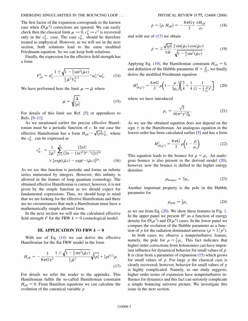
which E� V is nonnegative or p is larger than someminimal value and p0 is zero. The physical trajectorieslie in the nonshaded region bounded by a zero velocitycurve which represents a homoclinic orbit. Of course thewhole system is symmetric with respect to the reflection(H is changed in�H). The vertical (blue) line on the phaseportrait represents points at which trajectories pass hori-zontally through the inflection point (hyperinflationary/deflationary phases). Therefore, evolution comprises thebounce solution interpolating static phases of evolution,see Fig. 3. There is the intermediate phase of evolution atwhich we have the inflection point at the diagram of pðtÞ.Note that it is the singularity state with rapid growth of thescale factor, we call this phase the hyperinflation. It isimportant to note that energy density is finite during tran-sition through these singularities. Similar finite scale fac-tor singularities have been studied recently by Cannataet al. [13].In the phase diagram in Fig. 2 we adjoint a circle at

infinity in a standard way via Poincare construction. Notethat all trajectories are starting from an unstable node—representing a static Einstein universe and landing at astable node representing another static Einstein universe.Parisi et al. [14] pointed out that stability of Einstein

static models in high-energy modifications of general rela-tivity is important from the point of view of the so-calledemergent universe scenario [15]. Mulryne et al. [16] in-vestigated the stability of the Einstein static model and theyfound that the LQC Einstein static model is representing acenter type of critical point on the phase portrait. As it iswell known, such a critical point is structurally unstable.Note that in our case this static universe is representing a

FIG. 2 (color online). The phase portrait for all admissibleinitial conditions. The vertical (blue) line is representing pointsat which trajectories pass horizontally through the inflectionpoint (hyperinflationary/deflationary phases).

–4

–2

0

2

4

1 2 3 4ρ

–4

–2

0

2

4

1 2 3 4p

FIG. 1 (color online). Upper: Evolution of H2Oð�2Þ (red, bot-

tom curve) and H2Oð�4Þ (green, top curve) as a function of energy

density �. The parts below zero value of H2 are unphysical. The

� is in units of �c. Lower: Evolution of H2Oð�2Þ (red, bottom

curve) and H2Oð�4Þ (green, top curve) as a function of p for the

model with radiation (� / 1=p2). On both panels a physically

admissible region corresponds to H2 � 0.

JAKUB MIELCZAREK AND MAREK SZYDŁOWSKI PHYSICAL REVIEW D 77, 124008 (2008)

124008-4

node type of critical point. This modification of stability inthe presented model has important consequences for theemergent universe scenario, since as it is well known ingeneral relativity, a static universe is unstable and is rep-resented by a saddle type of critical point and therefore itrequires fine-tuning. Moreover, corrections consideredlead to a regularization of the big-bang singularity [17].

V. SUMMARY

In this paper we have calculated another nonvanishingcontribution to the quantum holonomy correction in loopquantum gravity. Quantum correction of this kind appearswhen we express the Ashtekar connection A and fieldstrength F in terms of holonomies. The source of quantummodification to classical expressions is a nonvanishing areaenclosed by a loop as the result of existence of the areagap �.

We had applied obtained corrections to the flat FRWcosmological model and then we calculated the result-ing quantum gravitational modifications to the Friedmannequation. The holonomy correction in the lowest order tothe flat FRW model was calculated earlier [5,18,19] andextensively studied [10,20]. These investigations uncov-ered existence of the bounce for energy scales �c. In thispicture the standard big-bang singularity is replaced by thenonsingular big bounce. Calculations performed in thepresent paper indicate that the holonomy correction inthe next nonvanishing order holds this picture. Namely,the initial singularity is still preserved. However thebounce appears now for higher energy density �bounce ¼3�c. Another important new feature is the appearance of apole in the Hubble parameter for �pole ¼ 3

2�c correspond-

ing to hyperinflationary/deflationary phases. This leads tomore complicated dynamical behavior at these energyscales.

We showed that the generic evolutional scenario for themodel with the free scalar field starts from the staticEinstein universe then recollapses passing through thecurvature singularity with a finite scale factor (hyperde-flation) towards the bounce and goes in the expandingphase through the second curvature singularity (hyperin-flation) and ends in the static Einstein universe. During thetransition through the singularities the universal criticalbehavior H / j�� �polej�1 holds. Therefore, in the pre-

sented scenario the bounce connects these two finite scalefactor singularities.As we see, the higher order quantum correction in LQG

can have an important influence on dynamical behavior ofcosmological models. It is not unlikely that the nonsingularbounce which appeared in the lowest order can be only anartifact of simplifications and can disappear when thewhole contribution will be taken into account. Furtherinvestigations of quantum corrections from LQG are stillnecessary. We conclude that higher order holonomycorrections and resulting different quantization schemesshould be also seriously taken into account inconsiderations.

ACKNOWLEDGMENTS

We thank Martin Bojowald for useful comments andprof. Jerzy Lewandowski and Łukasz Szulc for discus-sion during the workshop ‘‘Quantum Gravity in Cracow’’12-13.01.2008. Authors are grateful to Tomasz Stachowiakfor stimulating discussion. This work was supported in partby the Marie Curie Actions Transfer of Knowledge proj-ect COCOS (Contract No. MTKD-CT-2004-517186) andproject Particle Physics and Cosmology (Contract No.MTKD-CT-2005-029466).

APPENDIX: FLAT FRW MODEL IN LOOPQUANTUM GRAVITY

The FRW k ¼ 0 spacetime metric can be written as

ds2 ¼ �N2ðxÞdt2 þ qabdxadxb (A1)

where NðxÞ is the lapse function and the spatial part of themetric is expressed as

qab ¼ ij!ia!

jb ¼ a2ðtÞoqab ¼ a2ðtÞij

o!iao!j

b: (A2)

In this expression oqab is a fiducial metric and o!ia are co-

triads dual to the triads oeai ,o!iðoejÞ ¼ i

j whereo!i ¼

o!iadx

a and oei ¼ oeai @a. From these triads we constructthe Ashtekar variables

Aia �i

a þ �Kia ¼ cV�1=3

0o!i

a; (A3)

Eai

ffiffiffiffiffiffiffiffiffiffiffiffiffij detqj

qeai ¼ pV�2=3

0

ffiffiffiffiffioq

poeai ; (A4)

singularitiesscale factor

energy density

bounce

time

classical evolution

singularityclassical

quantum

quantumhyper−inflationhyper−deflation

FIG. 3 (color online). The schematic picture of the evolutionof the model. The top curve (green) represents the energy densityof the free scalar field. It is worth noting that this energy densityis finite during whole evolution, even during transitions throughsingularities. The bottom curve (blue) presents schematic evo-lution of the scale factor for the investigated model. The dashedcurve represents the classical evolution which is not realized inthe presented quantum model.

EMERGING SINGULARITIES IN THE BOUNCING LOOP . . . PHYSICAL REVIEW D 77, 124008 (2008)

124008-5

where

jpj ¼ a2V2=30 ; (A5)

c ¼ � _aV1=30 : (A6)

Note that the Gaussian constraint implies that p $ �pleads to the same physical results. The factor � is called the

Barbero-Immirzi parameter, � ¼ ln2=ð� ffiffiffi3

p Þ. In the defi-nition (A3) the spin connection is defined as

�ia ¼ ��ijkebj ð@½aekb� þ 1

2ecke

la@½celb�Þ; (A7)

and the extrinsic curvature is defined as

Kab ¼ 1

2N½ _qab � 2DðaNbÞ� (A8)

which corresponds to Kia :¼ Kabe

bi .

The scalar constraint, in the Ashtekar variables, hasthe form

HG ¼ 1

16�G

Z�d3xNðxÞ Ea

i Ebjffiffiffiffiffiffiffiffiffiffiffiffiffiffij detEjp

� ½"ijk kFkab � 2ð1þ �2ÞKi

½aKjb��; (A9)

where field strength is expressed as

Fkab ¼ @aA

kb � @bA

ka þ �kijA

iaA

jb: (A10)

With use of (A3), (A4), and (A10) the Hamiltonian (A9)assumes the form

HG ¼ � 3

8�G�2

ffiffiffiffiffiffiffijpj

qc2; (A11)

where we have assumed a gauge of NðxÞ ¼ 1. Quantumcorrections to this Hamiltonian come when we expressffiffiffiffiffiffiffijpjp

and c2 in terms of background-independent variables.

In this paper we have concentrated on the corrections to thefactor c2, called holonomy corrections. For a short reviewof quantum corrections we refer the reader to the appendixof Ref. [11].

[1] A. Ashtekar, Phys. Rev. D 36, 1587 (1987).[2] H. Nicolai, K. Peeters, and M. Zamaklar, Classical

Quantum Gravity 22, R193 (2005).[3] A. Perez, arXiv:gr-qc/0409061.[4] A. Ashtekar and J. Lewandowski, Classical Quantum

Gravity 14, A55 (1997).[5] A. Ashtekar, T. Pawlowski, and P. Singh, Phys. Rev. D 74,

084003 (2006).[6] M. Bojowald, Phys. Rev. D 75, 081301 (2007).[7] M. Bojowald, arXiv:0710.4919.[8] M. Bojowald, arXiv:0801.4001.[9] D.W. Chiou, Phys. Rev. D 76, 124037 (2007).[10] J. Mielczarek, T. Stachowiak, and M. Szydlowski,

arXiv:0801.0502.[11] J. Magueijo and P. Singh, Phys. Rev. D 76, 023510 (2007).[12] L. Perko, Differential Equations and Dynamical Systems

(Springer-Verlag, New York, 1991).[13] F. Cannata, A.Y. Kamenshchik, and D. Regoli,

arXiv:0801.2348.[14] L. Parisi, M. Bruni, R. Maartens, and K. Vandersloot,

Classical Quantum Gravity 24, 6243 (2007).[15] G. F. R. Ellis and R. Maartens, Classical Quantum Gravity

21, 223 (2004).[16] D. J. Mulryne, R. Tavakol, J. E. Lidsey, and G. F. R. Ellis,

Phys. Rev. D 71, 123512 (2005).[17] M. Bojowald, Phys. Rev. Lett. 86, 5227 (2001).[18] A. Ashtekar, T. Pawlowski, and P. Singh, Phys. Rev. Lett.

96, 141301 (2006).[19] A. Ashtekar, T. Pawlowski, and P. Singh, Phys. Rev. D 73,

124038 (2006).[20] P. Singh, K. Vandersloot, and G.V. Vereshchagin, Phys.

Rev. D 74, 043510 (2006).

JAKUB MIELCZAREK AND MAREK SZYDŁOWSKI PHYSICAL REVIEW D 77, 124008 (2008)

124008-6