emergent geometric organization and informative dimensions in
TRANSCRIPT

Emergent Geometric Organization and
Informative Dimensions in Coevolutionary
Algorithms
A Dissertation
Presented to
The Faculty of the Graduate School of Arts and Sciences
Brandeis University
Michtom School of Computer Science
Jordan B. Pollack, Advisor
In Partial Fulfillment
of the Requirements for the Degree
Doctor of Philosophy
by
Anthony Bucci
Aug, 2007

This dissertation, directed and approved by Anthony Bucci’s committee, has
been accepted and approved by the Graduate Faculty of Brandeis University
in partial fulfillment of the requirements for the degree of:
DOCTOR OF PHILOSOPHY
Adam B. Jaffe, Dean of Arts and Sciences
Dissertation Committee:
Jordan B. Pollack, Chair
Timothy J. Hickey
Marc Toussaint

c©Copyright by
Anthony Bucci
2007

To my parents, who gifted me with curiosity
and the stubbornness to follow where it leads.

Acknowledgments
It almost goes without saying that a piece of work this size could not have
been finished without the help of innumerable people. I wanted to extend my
gratitude to those who had the greatest impact on my thinking and writing
over the past eight years.
First, to my advisor Jordan Pollack. Jordan’s visionary quest for “mindless
intelligence,” a search for artificial intelligence without modeling the human
brain or mind, kept me engaged with a set of ideas and a set of people I would
otherwise never have encountered. Jordan’s enthusiasm and deep understand-
ing, not to mention his uncanny ability to direct attention to fertile areas of
research, are truly contagious and inspiring.
To Timothy Hickey and Marc Toussaint, who sat on my dissertation ex-
amining committee. Tim’s careful scrutiny uncovered what would have been
an embarrassing error. Marc, who has been interested in my work for several
years, painstakingly scoured the entirety of this dissertation, offering a myriad
small and large improvements along with suggestive interpretations of these
ideas from perspectives I had not considered.
v

vi
To past and present members of Jordan’s DEMO lab, including Ari Bader-
Natal, Keki Burjorjee, Edwin de Jong, Sevan Ficici, Simon Levy, Hod Lipson,
John Rieffel, Shiva Viswanathan, and Richard Watson. DEMO lab is a fecund
and stimulating research environment which contributed immeasurably to any
decent idea I had while there. Edwin, Sevan, Richard, and Shiva deserve spe-
cial mention. Edwin, whose unparalleled ability to implement complicated
algorithms and experiments have advanced the frontier of coevolutionary al-
gorithms research; I feel lucky to have had the opportunity to collaborate on
some of those efforts. Sevan, whose rigorous, careful thinking and understand-
ing of coevolutionary algorithms have served as a model for my own endeavors.
Shiva, for his thorough scholarship and for patient, thought-provoking discus-
sions. And Richard, whose infectious interest in Pareto coevolution, coupled
with a healthy disdain for unnecessary mathematics, both set me down this
path and kept my theorizing in check.
To friends and colleagues in the coevolutionary algorithms research com-
munity. I owe part of whatever meager knowledge I have of coevolutionary
algorithms to numerous conversations with Jeff Horn, Anthony Liekens, Liviu
Panait, Elena Popovici, Kenneth Stanley, and R. Paul Wiegand.
To the broader evolutionary computation community and those interested
in EC. I owe thanks to Ken De Jong, Sean Luke, Jon Rowe, Michael Vose, and
Abel Wolman, all of whom at one point or another graciously offered insights,
interest, or support for this work.
Finally, to Laura Chinchilla, whose light and faith guided me through some

vii
of my darkest moments. What would I have done without you?

Abstract
Emergent Geometric Organization and InformativeDimensions in Coevolutionary Algorithms
A dissertation presented to the Faculty ofthe Graduate School of Arts and Sciences ofBrandeis University, Waltham, Massachusetts
by Anthony Bucci
Coevolutionary algorithms vary entities which can play two or more distinct,
interacting roles, with the hope of producing raw material from which a highly-
capable composition can be constructed. Ranging in complexity from auto-
didactic checkers-learning systems to the evolution of competing agents in
3-d simulated physics, applications of these algorithms have proved both mo-
tivating and perplexing. Successful applications inspire further application,
supporting the belief that a correctly implemented form of evolution by nat-
ural selection can produce highly-capable entities with minimal human input
or intervention. However, the successes to date have generated limited insight
into how to transfer success to other domains. On the other hand, failed ap-
plications leave behind a frustratingly opaque trace of misbehavior. In either
case, the question of what worked or what went wrong is often left open.
One impediment to understanding the dynamics of coevolutionary algo-
rithms is that the interactive domains explored by these algorithms typically
lack an explicit objective function. Such a function is a clear guide for judg-
ing the progress or regress of an algorithm. However, in the absence of an
viii

ix
explicit yardstick to judge the value of coevolving entities, how should they be
measured?
To begin addressing this question, we start with the observation that in any
interaction, an entity is not only performing a task, it is also informing about
the capabilities of its interactants. In other words, an interaction can provide a
measurement. Entities themselves can therefore be treated as measuring rods,
here dubbed informative dimensions, against which other entities are incented
to improve. It is argued that when entities are only incented to perform well,
and adaptation of the function of measurement is neglected, algorithms tend
not to keep informative dimensions and thus fail to produce high-performing
entities.
It is demonstrated empirically that algorithms which are sensitized to these
yardsticks through an informativeness mechanism have better dynamic be-
havior; in particular, known pathologies such as overspecialization, cycling,
or relative overgeneralization are mitigated. We argue that in these cases an
emergent geometric organization of the population implicitly maintains infor-
mative dimensions, providing a direction to the evolving population and so
permitting continued improvement.

Contents
Abstract viii
1 Introduction 11.1 Performing and Informing . . . . . . . . . . . . . . . . . . . . 41.2 A Critique of Arms Races . . . . . . . . . . . . . . . . . . . . 6
1.2.1 Does Competition Help? . . . . . . . . . . . . . . . . . 71.2.2 Does Cooperation Help? . . . . . . . . . . . . . . . . . 15
1.3 The Problem of Measurement . . . . . . . . . . . . . . . . . . 211.4 Conceptual Background . . . . . . . . . . . . . . . . . . . . . 28
1.4.1 Evolutionary Algorithms . . . . . . . . . . . . . . . . . 281.4.2 Evolutionary Multi-objective Optimization . . . . . . . 291.4.3 Coevolutionary Algorithms . . . . . . . . . . . . . . . . 301.4.4 Pareto Coevolution . . . . . . . . . . . . . . . . . . . . 34
1.5 Overview . . . . . . . . . . . . . . . . . . . . . . . . . . . . . . 401.5.1 Perspective on Ideal Trainers . . . . . . . . . . . . . . 44
2 Mathematical Preliminaries 462.1 Ordered Sets . . . . . . . . . . . . . . . . . . . . . . . . . . . 462.2 Functions into Ordered Sets . . . . . . . . . . . . . . . . . . . 512.3 Poset Decomposition . . . . . . . . . . . . . . . . . . . . . . . 54
3 Informative Dimensions 573.1 Overview . . . . . . . . . . . . . . . . . . . . . . . . . . . . . . 573.2 Static Dimension Selection and Intransitivity . . . . . . . . . . 58
3.2.1 The Framework . . . . . . . . . . . . . . . . . . . . . . 603.2.2 Pareto Dominance and Intransitivity . . . . . . . . . . 693.2.3 Discussion . . . . . . . . . . . . . . . . . . . . . . . . . 73
3.3 Static Dimension Extraction . . . . . . . . . . . . . . . . . . . 74
x

CONTENTS xi
3.3.1 Geometrical Problem Structure . . . . . . . . . . . . . 753.3.2 Dimension-Extraction Algorithm . . . . . . . . . . . . 843.3.3 Experiments . . . . . . . . . . . . . . . . . . . . . . . . 863.3.4 Discussion . . . . . . . . . . . . . . . . . . . . . . . . . 89
3.4 Discussion . . . . . . . . . . . . . . . . . . . . . . . . . . . . . 90
4 Emergent Geometric Organization 944.1 Overview . . . . . . . . . . . . . . . . . . . . . . . . . . . . . . 944.2 Dynamic Dimension Selection and Underlying Objectives . . . 98
4.2.1 Orders and Coevolution . . . . . . . . . . . . . . . . . 994.2.2 Experiments . . . . . . . . . . . . . . . . . . . . . . . . 1044.2.3 Discussion . . . . . . . . . . . . . . . . . . . . . . . . . 112
4.3 Dynamic Dimension Selection and Relative Overgeneralization 1124.3.1 Background . . . . . . . . . . . . . . . . . . . . . . . . 1144.3.2 Analysis . . . . . . . . . . . . . . . . . . . . . . . . . . 1204.3.3 Experiments . . . . . . . . . . . . . . . . . . . . . . . . 1264.3.4 Discussion . . . . . . . . . . . . . . . . . . . . . . . . . 128
4.4 Discussion . . . . . . . . . . . . . . . . . . . . . . . . . . . . . 129
5 Conclusions, Critiques and Corollaries 1325.1 Dynamic Dimension Extraction . . . . . . . . . . . . . . . . . 1415.2 Extracted Dimensions Are Not Trivial . . . . . . . . . . . . . 1425.3 Informative Actions in CCEA . . . . . . . . . . . . . . . . . . 1455.4 Estimation-Exploration Algorithm . . . . . . . . . . . . . . . . 1475.5 Solution Concepts . . . . . . . . . . . . . . . . . . . . . . . . . 1495.6 Pathologies Revisited . . . . . . . . . . . . . . . . . . . . . . . 151
5.6.1 Resource Consumption . . . . . . . . . . . . . . . . . . 1515.6.2 Disengagement and Stalling . . . . . . . . . . . . . . . 1525.6.3 The Later is Better Effect . . . . . . . . . . . . . . . . 155
Bibliography 156

List of Tables
1.1 A simple payoff matrix illustrating why averaging or maximizingpayoff can be misleading. . . . . . . . . . . . . . . . . . . . . . 22
1.2 Rosin’s competitive fitness sharing calculation applied to thematrix in table 1.1. . . . . . . . . . . . . . . . . . . . . . . . . 23
4.1 Values of f1 and f2 on four points in the xy-plane spanning asquare which lies under the higher-valued peak. . . . . . . . . 122
4.2 Comparison of CCEA, cCCEA, and pCCEA on MTQ1. . . . . 1274.3 Control experiment comparing cCCEA and pCCEA on MTQ2. 128
xii

List of Figures
1.1 CIAO plot illustration. . . . . . . . . . . . . . . . . . . . . . . 111.2 Two hypothetical dynamics indistinguishable by CIAO plots
but distinguishable by AOG plots. . . . . . . . . . . . . . . . . 141.3 An illustration of how outcomes against one set of entities can
be used as objectives for another set, and the resulting non-dominated front. . . . . . . . . . . . . . . . . . . . . . . . . . 36
2.1 ≤pw and ⊆ can be distinct orders on [S → R]. Let S = {a, b},R = {0 < 1 < 2}. Observe that f1 ≤pw f2, but f1 6⊆ f2; and,f2 ⊆ f3, but f2 6≤pw f3. . . . . . . . . . . . . . . . . . . . . . . 53
3.1 Typical members of the families X and Y; see text for details. 773.2 Algorithm for coordinate system construction. . . . . . . . . . 923.3 Estimated number of dimensions in two numbers games, apply-
ing the algorithm in fig. 3.2. . . . . . . . . . . . . . . . . . . . 93
4.1 The preorder rock-stone-paper-scissors displayed as a graph. . 1024.2 The preorder rock-stone-paper-scissors pseudo-embedded into
the plane� 2 . . . . . . . . . . . . . . . . . . . . . . . . . . . . 103
4.3 Performance versus time of P-CHC and P-PHC on IG (intran-sitive game). . . . . . . . . . . . . . . . . . . . . . . . . . . . . 109
4.4 Performance of P-CHC and P-PHC on FG (focusing game). . 1104.5 Position in plane of final candidates from P-CHC run on pFG,
together with final candidates and tests from P-PHC. . . . . . 1114.6 Plot of MTQ1. . . . . . . . . . . . . . . . . . . . . . . . . . . 1184.7 Plot of MTQ2. . . . . . . . . . . . . . . . . . . . . . . . . . . 1184.8 Plot of candidates y∗ and y∗ as cross sections through MTQ1. 1244.9 Cross sections through MTQ1 defined by two different Y values. 125
xiii

Chapter 1
Introduction
This dissertation is concerned with a hope expressed by Arthur Samuel in his
influential work on machine learning. Samuel writes:
We have at our command computers with adequate data-handling
ability and with sufficient computational speed to make use of
machine-learning techniques, but our knowledge of the basic prin-
ciples of these techniques is still rudimentary. Lacking such knowl-
edge, it is necessary to specify methods of problem solution in
minute and exact detail, a time consuming and costly procedure.
Programming computers to learn from experience should eventu-
ally eliminate the need for much of this detailed programming effort
[93].
Recall that Samuel’s procedure learned an evaluation function for check-
ers board configurations which could then be used as a checkers player using
1
CHAPTER 1. INTRODUCTION 2
lookahead search. The evaluation function was represented as a weighted sum
of hand-constructed board features. The learning procedure learned which
terms should be present in the function as well as the weights of each term.
The self-play procedure kept a learner, Alpha, and played it against a test op-
ponent Beta. After some number of steps training Alpha, during which Beta
remained frozen, Alpha was copied to Beta and learning repeated. Thus the
test opponent Beta was always a frozen copy of the learner. The procedure
produced checkers players which were better than the average human player
[93].
Samuel’s method for learning checkers by self-play can be interpreted as
a simple coevolutionary algorithm. The Alpha player, which is changing with
experience, is pitted against the Beta player, which is frozen and used as a
measurement of Alpha’s abilities:
At the end of each self-play game a determination is made of the
relative playing ability of Alpha, as compared with Beta, by a
neutral portion of the program [93].
To elaborate the analogy with evolutionary computation, Samuel’s proce-
dure can be called a coevolutionary algorithm with two populations of size
1, asynchronous population updates, and domain-specific, deterministic vari-
ation operators. If this analogy between learning by self-play and coevolu-
tionary algorithms is taken seriously, Samuel’s enthusiasm for self-play pre-
figures the expressed belief that a properly configured coevolutionary pro-
CHAPTER 1. INTRODUCTION 3
cess can produce highly capable and complex entities in interactive domains
[96, 87, 69, 82, 45, 40, 39, 97, 99] without the need for “detailed programming
effort” beyond setting up the evolutionary algorithm itself.
Our aim in this chapter is to assess that hope in light of prior work. We will
conclude that while the hope is alive, existing methods are far from achieving
the general-purpose coevolutionary arms race which, until now, has been taken
as a guiding conception of a successful coevolutionary process. We ask: why
not? We hypothesize that the reason arms races have been difficult to induce
rests on two general trends in previous work:
1. The use of a single, numerical fitness value to compare entities;
2. The derivation of fitness from interactions with a pool of entities which
were incented to perform at a task, rather than to inform about the
abilities of other entities.
This dissertation argues that changing fitness values to be multi-objective
rather than single numerical values, and explicitly incenting individuals to
inform, can remedy two known impediments to inducing arms races, namely
overspecialization and cycling. The same move impacts and mitigates a pathol-
ogy in so-called cooperative coevolutionary algorithms where the arms race
conception has not been influential but nevertheless appears in a slightly al-
tered form. Taken together, these observations suggest that the conventional
view of arms races, broadly interpreted to encompass cooperative coevolution-
ary algorithms, may indeed be to blame for unsatisfactory algorithm perfor-

CHAPTER 1. INTRODUCTION 4
mance. To further bolster that claim, we prove theoretically that a wide class
of interactive domains possess implicit informative dimensions which func-
tion as measurements or objectives for performing entities. Generally there
is more than one such dimension (again yielding a multi-dimensional notion
of value), and they are unknown to a coevolutionary algorithm a priori. We
observe empirically that explicitly incenting certain entities to inform leads to
an emergent geometric organization of the informing entities into a represen-
tation of informative dimensions, thereby ensuring increases in performance
by providing the information backdrop against which such increases can be
measured. Failure to maintain informative dimensions can, and does, lead to
algorithm misbehavior. Thus, we propose an alternate conception of the aim
of a coevolutionary algorithm: instead of creating and sustaining an arms race,
an algorithm should simultaneously discover and ascend informative dimen-
sions.
The following sections motivate the need for work on this topic, detail the
conceptual background of these claims and give an overview of the argument.
1.1 Performing and Informing
Samuel exposes a split in roles which will be the central concept of this disser-
tation. The Alpha player, which is in a learning mode, is incented to perform
well at playing checkers. By contrast, the frozen Beta player, by functioning
as a measurement of Alpha’s play, is intended to inform well about Alpha’s

CHAPTER 1. INTRODUCTION 5
performance. The two roles are treated differently in Samuel’s learning algo-
rithm, with good reason: one would expect that even the strongest learning
algorithm will fail without a “trustworthy criteria for measuring performance”
[93].
While Samuel’s work describes learning against a measurement function in
detail, it does not aim to directly address the simultaneous adaptation of the
function of measurement. Rather than arising from a similarly complicated
assessment procedure, the Beta player is simply a copy of Alpha, frozen after
one cycle of learning and used as a fixed measurement in the next cycle. The
mechanism hinges on the conceit that as Alpha’s play improves, it also becomes
a better and better measurement of checkers play such that a copy of it suffices
to test future variations arising during learning. Similar mechanisms have been
employed in learning backgammon strategies [100, 82] as well as evolving the
morphology and behavior of 3-d simulated creatures [96].
A similar conceit has seen expression in the notion of a coevolutionary
arms race [28, 39, 72] in which two types of entity are locked in an escalating
struggle for dominance. The theory goes that as one type of entity improves,
the other type must simultaneously improve as well to avoid extinction or
stagnation. This algorithmic analog of the Red Queen Effect [101] is envisioned
as the hallmark of an ideal coevolutionary process. One may well believe
that if algorithms could be designed to maintain arms races, then they would
eventually, if not quickly, produce the entities best adapted to do well in the
interactive domain to which they are applied.

CHAPTER 1. INTRODUCTION 6
1.2 A Critique of Arms Races
Unfortunately, the arms race conception does not hold up to harder scrutiny,
for the simple reason that performing is not the same as informing. The
distinction between these two roles will be explored more carefully in chapter
3, section 3.2.1, which argues that these two roles can be quite different some
domains; and again in chapter 4, section 4.3.2, which argues that in other
domains, the two roles may indeed coincide to some degree. Here, consider a
criticism from the domain of learning games of strategy. Susan Epstein argues
that
Teaching a program by leading it repeatedly through the same
restricted paths, albeit high quality ones, is overly narrow prepa-
ration for the variations that appear in real-world experience. A
program that directs its own training may overlook important sit-
uations [37].
Epstein points out that a naıve application learning by self-play to game
strategy domains can lead to brittle strategies because the procedure has a
tendency to ignore large swathes of the game’s configuration space. Her ob-
servation hearkens back to Donald Michie’s experience with the MENACE
Tic-Tac-Toe learning procedure that training against a perfect Tic-Tac-Toe
player did not lead MENACE to a strong Tic-Tac-Toe strategy [65]. A re-
lated observation about the strength of coevolved Tic-Tac-Toe players has
also been made: evolving against a fixed strategy tends to produce brittle

CHAPTER 1. INTRODUCTION 7
strategies, a shortcoming which a coevolutionary algorithm can alleviate [2].
These works suggest that carefully selecting the opponents against which a
strategy is tested, in other words controlling how informing is done, has a
significant impact on the quality of the learned strategy.
Therefore, Samuel’s mechanism of using a copy of Alpha as a measure-
ment of Alpha’s later progress, while successful in learning checkers players,
backgammon strategies, or creature behavior, is not of general applicability.
Nevertheless, a variety of coevolutionary algorithms use a mechanism essen-
tially like Samuel’s to provide fitness information during evolution. In a typical
two-population coevolutionary algorithm, entities in one population are eval-
uated by interacting with entities from the other. They are then assigned a
fitness value intended to reflect their performance. Since entities are selected
on the basis of their fitness, the pool of entities which can be used as fitness
measurements via interaction has arisen from an incentive to perform well. If
both populations are adapting to performing the same task, as in [96, 100, 82],
then we have a mechanism much like Samuel’s, but elevated (at least in [96])
to populations of entities rather than individual entities.
1.2.1 Does Competition Help?
What if one set of entities is incented to perform well, while the other is
incented to make that difficult? In other words, instead of having two popu-
lations of entities, each of which is incented to excel at the task, why not have
one set attempt to perform well while the other attempts to stump, beat, or
CHAPTER 1. INTRODUCTION 8
otherwise expose shortcomings of the first? This kind of evolutionary zero-sum
game [64, 49] differs from Samuel’s mechanism by attaching different incentive
structures to the two different roles of performing and informing. In coevolu-
tionary algorithms research, this idea has arisen in several forms: for instance,
in coevolving abstract hosts and parasites [51, 40, 74, 81, 23, 4], pursuit and
evasion strategies [89, 66, 26, 72, 54], classifiers and test cases [57, 79, 59], func-
tion regression [75], robotics [73, 72, 45], and of course game strategy learning
[2, 92, 4, 24].
These methods have collectively been referred to as competitive coevolu-
tion [2, 89, 92, 45]. A feature they share is that the assessment of an entity in
one population is summarized in a composite number, the fitness, produced
by integrating over its interaction outcomes with individuals from the other
population. The integration may be by averaging, a weighted average, max-
imization, or more sophisticated methods. Nevertheless, entities are always
given a single numerical fitness which is used to decide which entities are bet-
ter.
Because of its aim to find “the best,” the line of work on competitive co-
evolution is replete with reactions against well-known pathological behavior
which call the lie on the arms race conception. Rather than finding the best
entities, straightforward applications of competitive coevolutionary techniques
frequently produce poor individuals and confusing dynamics. Behaviors such
as disengagement, cycling, overspecialization/focusing, and evolutionary for-

CHAPTER 1. INTRODUCTION 9
getting1 have all arisen often enough in applications that specific remedies
have been proposed for each.
Pathologies
To cite two examples of well-known pathologies:
Disengagement occurs when one population of entities provide no informa-
tion about the quality of the other coevolving entities. Rosin and Belew’s phan-
tom parasite [90], Juill’e and Pollack’s fitness sharing [58], Olsson’s method of
freezing one population until the other has evolved to beat all individuals in it
[74], Paredis’s X method [80], and Cartlidge and Bullock’s modulating para-
site virulence [23] have all been observed to prevent disengagement in certain
special cases.
Cycling, wherein the algorithm revisits the same points over and over again,
sometimes gaining and sometimes losing ground, has received considerable at-
tention. [22], for example, proposes “diffuse” coevolution, which essentially
increases the number of populations, as a remedy to cycling. Hornby and Mir-
tich [54] follows up this work, also using a robotics domain. Rosin and Belew,
by contrast, recommends a competitive fitness sharing mechanism which dis-
counts the fitness given to entity A interacting with B by the fitness all other
entities receive against B [92]. Juill’e and Pollack propose a similar mecha-
nism, where an entity receives a fitness bonus for doing well against opponents
which other entities cannot defeat [57]. Nolfi and Floreano observe that cycling
1See [103] for a survey of these.

CHAPTER 1. INTRODUCTION 10
tends to be damped with obstacles and walls are added to the environment of
coevolving pursuing/evading robots [72]. This last work raises the question of
whether arms races really can arise in competitive coevolution.
The identification of these various algorithmic misbehaviors has led to a
considerable amount of work focused on remedying them or monitoring the
progress of an algorithm while it is running, serving the aim of forcing an
arms race to occur. A summary of key work follows.
Remedies
Karl Sims’s best elite opponent technique [96] provides the inspiration for many
subsequent mechanisms. In Sims’s algorithm, simulated robots are pitted
against one another in a duel over a cube. Robots receive fitness boosts for
each moment they spend in contact with the cube while their opponent is not.
Sims uses a fitness metric based on how many opponents a robot beats to de-
cide which were the elites – that is, the best – in a population. At subsequent
generations, individuals are tested against (compete with) the best elite of the
previous generation.
Rosin’s hall of fame mechanism [91] accumulates the best individual from
each generation. Subsequent generations are then tested against a random
sample from the hall of fame. The intuition is that by broadening testing
to include former best individuals, an algorithm can maintain a direction for
coevolution.
In the sphere of monitoring progress, Cliff and Miller’s CIAO (Current
CHAPTER 1. INTRODUCTION 11
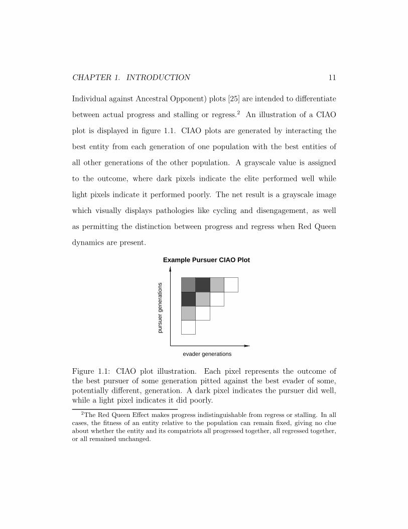
Individual against Ancestral Opponent) plots [25] are intended to differentiate
between actual progress and stalling or regress.2 An illustration of a CIAO
plot is displayed in figure 1.1. CIAO plots are generated by interacting the
best entity from each generation of one population with the best entities of
all other generations of the other population. A grayscale value is assigned
to the outcome, where dark pixels indicate the elite performed well while
light pixels indicate it performed poorly. The net result is a grayscale image
which visually displays pathologies like cycling and disengagement, as well
as permitting the distinction between progress and regress when Red Queen
dynamics are present.
purs
uer
gene
ratio
ns
evader generations
Example Pursuer CIAO Plot
Figure 1.1: CIAO plot illustration. Each pixel represents the outcome ofthe best pursuer of some generation pitted against the best evader of some,potentially different, generation. A dark pixel indicates the pursuer did well,while a light pixel indicates it did poorly.
2The Red Queen Effect makes progress indistinguishable from regress or stalling. In allcases, the fitness of an entity relative to the population can remain fixed, giving no clueabout whether the entity and its compatriots all progressed together, all regressed together,or all remained unchanged.

CHAPTER 1. INTRODUCTION 12
The master tournament of Nolfi and Floreano [44] takes the CIAO plot
one step further. After a run of an algorithm, a tournament is run amongst
the best of each population. That is, while CIAO plots compare the elite
pursuers against the elite evaders, the master’s tournament compares all the
elite pursuers against one another (and symmetrically, all the elite evaders
against one another). Thus, in addition to the information about cycling
and disengagement perceivable from a CIAO plot, the master’s tournament
permits one to see at which generation an innovation occurred in the pursuer
behavior. If, for instance, the elite pursuer from generation 100 is able to defeat
the elite pursuers from all previous generations in the master’s tournament,
the pursuer population apparently made some advance in pursuit behavior.
Similar, symmetric remarks apply to the evaders.
Techniques aimed at alleviating cycling behavior include diffusing entities
across multiple populations [22, 54] as well as dispersing them on a spatial
grid [51, 75]. Introducing obstacles [72] to the task domain has been reported
to dampen cycling behavior as well.
Disengagement, by contrast, is often attacked by allowing low-fit individu-
als a chance to survive to future generations. The intuition mirrors Minsky’s
discussion of hillclimbing in [67], which notes the tendency for such algorithms
to become stuck on what he terms mesas 3 or local optima. Algorithms which
keeps sub-par individuals may be able to escape such dead ends. The lesson
is that consolidating too quickly around what presently seem to be the best
3Plateaus in the evolutionary computation parlance.

CHAPTER 1. INTRODUCTION 13
individuals can lead to a lack of diversity and thus limited options for escaping
sub-optimal but dynamically-stable solutions. Competitive fitness sharing and
phantom parasites [90], Juille’s fitness sharing [59], and Cartlidge’s modulating
parasite virulence [23] re-weight the fitness of entities, whereas Olsson’s algo-
rithm [74] and Paredis’ X method [80] alter the rate at which populations are
updated, effectively delaying the time at which low-fit entities are discarded.
What’s in a Number?
It should be emphasized that all the mechanisms thus far surveyed rely on a
single numerical fitness value for entities, elaborating on but otherwise follow-
ing Sims’s best elite opponent conception [96]. In all cases the best individuals
are determined on the basis of this single number.
An exception is Bader-Natal’s all of generation (versus best of generation)
technique [6, 7]. An AOG plot resembles the CIAO plot. Rather than plotting
a pixel representing the outcome of the best entity of one population against
the best entity of the other, the AOG method plots a pixel summarizing the
interactions of entities in one population with those of the other. As with
CIAO, AOG plots can be used to detect cycling and disengagement as well as
to differentiate progress from regress when Red Queen dynamics are at play.
However, they additionally permit distinguishing two dynamics illustrated in
figure 1.2.
Thus, one advantage of an AOG method is that it can predict a potential
collapse in ability: if all but the best entity are decreasing in capability, effects

CHAPTER 1. INTRODUCTION 14
average
best
time
fitn
ess
best
time
fitn
ess
average
Figure 1.2: Two hypothetical dynamics indistinguishable by CIAO plots butdistinguishable by AOG plots. In both examples, the best individual takes thesame, increasing trajectory through fitness space. However, the average fitnessof the population is different, increasing in the left plot while decreasing in theright one.
like drift or noise might lead to the loss of that best and produce a catastrophic
decrease in the abilities represented in the population.
Summary
After surveying this much work on pathological algorithm behavior and pro-
posed remedies, a natural conclusion is that arms races are the exception
rather than the rule in competitive coevolution. If that is truly the case, then
perhaps another approach is warranted.
Rosin notes:
In competitive coevolution, we have two distinct reasons to save
individuals. One reason is to contribute genetic material to future
generations. Selection serves this purpose. The second reason to
save individuals is for the purposes of testing [91].
CHAPTER 1. INTRODUCTION 15
Rosin’s statement suggests the implicit belief that testing well arises nat-
urally from performing well. As with Samuel’s work, the pool of entities from
which tests are drawn, even if they come from a hall of fame, ultimately arises
from incentives to perform well. If this same belief truly lies behind work
identifying and studying coevolutionary pathologies, then perhaps the conceit
that informing is tantamount to performing is to blame. Furthermore, since
the reliance on single numerical fitness values for identifying best elite oppo-
nents is common to all experiments reporting pathological dynamics, perhaps
the reliance on numerical fitnesses should also be questioned.
1.2.2 Does Cooperation Help?
Cooperative coevolution refers to a class of coevolutionary algorithms intended
to optimize functions. Though the ideas of this class of algorithm are present
in [55], the term cooperative coevolution as it is used today is introduced in
[87]. The key idea behind this class of algorithms is to decompose potential
solutions into component parts, then test each component in the context of
an assembly built from other, coevolving parts (see [19], which elaborates this
test-based point of view). Each type of part is ensconced in its own population
and evolved separately using standard evolutionary computation techniques.
However, at the time when a part is to be evaluated, it is coupled with parts,
called collaborators from other populations to produce a working whole which
can be input to the objective function. Typically, parts are coupled with the
best (that is, highest-fitness) entities from the other populations, as well as

CHAPTER 1. INTRODUCTION 16
with randomly-selected entities. In general, there is a problem of collaborator
selection: exactly which other entities should be used to assess a given part?
The ultimate fitness given to the part is the maximum or average of the values
it received in the various assemblies in which it was assessed. That fitness is
used to make selection decisions and produce the next population.
Cooperative coevolutionary algorithms (CCEAs) have not typically been
associated with notions of arms race. Arms races are traditionally associated
with competitive coevolutionary algorithms. Yet it can already been seen that
cooperative coevolutionary algorithms share a number of features in common
with their competitive counterparts which make them worth considering from
the same perspective. For instance, CCEAs rely on single numerical fitness
values, the determination of best or elite entities from these numbers, and the
use of composites like maxima or averages to determine the fitness value.
Since the value of such mechanisms was critiqued in section 1.2.1, what are
we to make of their use in cooperative coevolutionary algorithms? Does the
cooperative nature of the evaluation, wherein parts are incented to perform
well with other parts rather than defeat them, make a difference to the argu-
ment of the previous section? Here we suggest it does not by surveying the
debate over collaboration methods and a pathology known as relative over-
generalization. We raise the question of whether the conflicting observations
of which collaboration method is most successful (and why), as well as the
relative overgeneralization phenomenon, can both be explained in terms of
inadequate testing of parts.

CHAPTER 1. INTRODUCTION 17
Collaboration Methods
When the objective function used in a cooperative coevolutionary algorithm is
separable in the sense that each component part has a fitness value independent
of the other parts, a coevolutionary algorithm is not necessary. Each type of
part can be independently evolved to a high level of fitness, and then the
highest-fitness entities can be combined into a whole which is guaranteed to
also be high fitness. Consequently, most attention has been paid to domains
which do not possess such a simple objective function. While a full survey of
the discussion over collaboration methods which has appeared in the literature
is beyond the scope of the present endeavor, we will focus on one line of work
regarding cross-population epistasis and several techniques which have been
used to study it.
In more complicated domains, it can happen that a part may appear to
have a high value when it is combined with one collaborator, but then appear
to have a poor value when it is combined with some other collaborator. As a
simple illustration, a charged AA battery has high value in a remote control
which takes AA batteries, but has almost no value in a remote control which
takes AAA batteries. A more formal example of this effect is analyzed in
chapter 4, section 4.3.
The broader observation of cross-population epistasis, of which the AA
battery example is a simple illustration, is the rule rather than the excep-
tion. Intuitively speaking, in the presence of such an effect, one must carefully
CHAPTER 1. INTRODUCTION 18
choose which collaborators are utilized to assess a given part. However, the
empirical analysis in [107] brings that intuition into question by demonstrating
that cross-population epistasis alone does not always necessitate complicated
collaboration schemes. [106], also an empirical study, furthers that work to
suggest that contradictory cross-population epistasis, of which the AA illustra-
tion is also a simplified example, has a stronger effect on which collaboration
method leads to successful coevolution.
Popovici and De Jong [83] have constructed a class of test functions which
contradict this conclusion. While all the test functions have contradictory
cross-population epistasis, the single-best collaboration method used in the
tested CCEA performs well in some cases but poorly in others. To explain
this difference, the authors apply two techniques. First is a dynamical systems
analysis technique first presented in [105] which tracks the trajectory of the
best individual of one or more of the populations through time (see also [85]).
The other is a notion of best response curves given in [86] which plots, for
each entity in one population, the entity in the other population with which
the first would receive its highest payoff.4 One conclusion drawn from these
studies is that if the trajectory of the best entity lands at the intersection of the
best response curves, then the algorithm has become stuck. These intersection
points are, in fact, Nash equilibria: since each entity is paired with the entity
with which it does best (hence the name best response curve), no entity has
4The authors note that this information is only available for simple test problems suchas those given in [84]; though the best response curves are not known in advance in hardproblems, and in fact may not even be curves, they demonstrably provide theoretical insight.

CHAPTER 1. INTRODUCTION 19
an incentive to change.
It should be stressed that the dynamical systems technique of tracking the
trajectory of the single best entity which runs through this line of work also
relies on a single, numerical fitness value. The best entity is identified by its
fitness, which is computed as an aggregate of its collaborations with entities in
another population. Compare the discussion of AOG plots in section What’s
in a Number, and in particular figure 1.2.
Pathology
Relative overgeneralization, as treated in [105], refers to the tendency of coop-
erative coevolutionary algorithms to prefer parts which perform suboptimally
in a large variety of assemblies, versus preferring parts which are present in
the globally optimal assemblies. The identification of this pathology in test
domains such as the class of maximum of two quadratics functions [105] contra-
dicts the intention expressed in [87] that cooperative coevolutionary algorithms
optimize functions.
A possible remedy to this pathology is proposed in [78]. Rather than
assessing a part only in the context of best or randomly-chosen parts, this
work suggests biasing the part’s assessment towards what it would be in the
context of parts which would appear in the global optima. Naturally, such
information is not available to a running algorithm; if it were, there would be
no need for coevolution.5 Nevertheless, the authors argue that if an estimate
5If we could obtain the optimal assessment of each instance of each type of part, we could

CHAPTER 1. INTRODUCTION 20
of the optimal assessment is available, it can be used to bias the evaluation of
parts and thus bias the algorithm towards the globally optimal solutions.
Once again, it cannot be overstressed that the identification of best enti-
ties comes from a single numerical fitness value computed as an aggregate of
interactions with members of other populations.
Summary
In short, the belief implicit in CCEA research has been that when exploring
a domain that involves cooperation, being good in an assembly is the best
way to inform about how good a component is. Credit assignment [70, 67]
to a part is done by testing that part in wholes made with other collabo-
rating parts. Often, the collaborators chosen are the best ones previously
encountered. CCEA work recognizes the shortcoming of this testing mode
by including random collaborators; a continuing debate has questioned which
of several possible collaborator selection methods works best. Furthermore,
if one seeks to optimize a function, as cooperative coevolutionary algorithms
were originally intended to do, the relative overgeneralization phenomenon be-
comes an undesirable algorithm behavior which is to be avoided [105]. Thus
far, the only technique available for avoiding relative overgeneralization has
been to bias the assessment of a part towards what its optimal assessment
would be, information which is generally unavailable to a running algorithm.
independently evolve the parts using this information as the objective. Several independentevolutionary algorithms would suffice for this task, obviating the need for a coevolutionaryalgorithm.
CHAPTER 1. INTRODUCTION 21
Notice that the pool of parts from which collaborator choices are made
have been incented to perform well. Further, note that Epstein warns against
using random choices for tests: “variety introduced into training by random
choice is unreliable preparation” [37].
Thus, the issues raised in section 1.2.1 concerning the shortcomings of
single numerical fitness assessments coming from interactions with performers
are just as relevant to cooperative coevolutionary algorithms as they are to
competitive ones, even if cooperative coevolutionary have not traditionally
been regarded as seeking arms races. Could it be that the lack of consensus
on collaboration methods and the relative overgeneralization pathology also
arise from uninformative testing?
1.3 The Problem of Measurement
To sum up where we have come so far, we have seen three broad classes of
testing or measuring methods in use in coevolutionary algorithms. First, we
considered methods like Samuel’s checkers learner, which use best-performing
players as tests of variations of the performing entities. Second, we discussed
competitive coevolutionary methods which inform about performing individu-
als by in some sense attacking their capabilities with other performers. Third,
we surveyed cooperative coevolutionary techniques which assign credit to en-
tities by assembling them into wholes and observing how well the whole does.
We found that in spite of compelling successes in particular domains, in general

CHAPTER 1. INTRODUCTION 22
brittleness, cycling and disengagement, or relative overgeneralization, respec-
tively plague the three approaches.
The overarching, motivating question of this dissertation is: could there be
a common cause to all these misbehaviors? Rather than being specific failings
of specific techniques in specific domains, could these failings all be the result
of the consolidation of interaction information into a single numerical fitness
value? Could the information loss entailed by such an integration be the
culprit? Moreover, since virtually all surveyed techniques test with entities
which were previously incented to perform, could it help to truly separate
these two roles and draw tests from entities which were directly incented to
inform? In other words, could there be a universal problem of measurement?
In order to flesh out the problem more fully, the next section gives reasons
to believe that aggregating in general is a poor choice of measurement. The
subsequent section outlines what might be done instead.
Why Are Aggregates Bad Measurements?
Consider the payoff matrix displayed in table 1.1.
t u v w max avga 100 0 0 0 100 25b 0 1 1 1 1 3
4
c 0 0 3 0 3 34
Table 1.1: A simple payoff matrix illustrating why averaging or maximizingpayoff can be misleading.
A note about terminology. Let us identify the set S = {a, b, c} as the

CHAPTER 1. INTRODUCTION 23
candidate solutions for the problem represented by this payoff matrix. The
intention is to find one or more members of S which are “good” in some sense.
Dually, let us identify the set T = {t, u, v, w} as test entities which provide
information about the candidate entities by interacting with them. Previously
we drew a distinction between performing and informing; that distinction is
instantiated here by asserting the candidate solution role is to perform, while
the test entity role is to inform.
The ranking of the entities S = {a, b, c} entailed by taking their maximum
payoff against T = {t, u, v, w} is a > c > b. The ranking entailed by taking
their average is a > b, a > c, and b = c. The two aggregation methods conflict
in the relative merits of b and c, but both agree that a is the best entity in S.
Now consider a more complicated example, the competitive fitness shar-
ing method described in [92]. Using that method, we derive the competitive
fitnesses show in table 1.2.
t u v w shared fitnessa 100 0 0 0 100
100= 1
b 0 1 1 1 1 + 14
+ 1 = 214
c 0 0 3 0 34
= 34
sum 100 1 4 1
Table 1.2: Rosin’s competitive fitness sharing calculation applied to the matrixin table 1.1.
Competitive fitness may change the ranking of individuals. Here, the rank-
ing given is b > a > c. In particular, a is no longer considered best; b is.
Further, where before c had at worst an ambiguous position in the ranking,

CHAPTER 1. INTRODUCTION 24
here c is definitively the worst entity.
Indeed, a variety of re-weightings of payoff values can and have been imag-
ined. The various weighting methods will often conflict in how they rank
entities, just as max, average, and competitive fitness sharing conflict. We are
assured of that conclusion by Arrow’s impossibility theorem [3].
To see this, think of each of the entities in T as producing a ranking of the
entities in S, a point of view we will explore more fully in chapter 3. In some
sense each test in T is voting on how it believes S should be ranked. Any
aggregate like max or average which produces a single numerical value also
produces a ranking of S. For example, we saw that max produces the ranking
a > c > b. Framed this way, the question of aggregating payoffs is precisely the
question of making social choice from individual values which Arrow’s book
treats. Mapped to the present context, Arrow’s impossibility theorem states
that under conditions when two tests conflict in how they rank entities, any
aggregate of the payoffs which is also a rank will conflict with at least one of
the tests.
Note in table 1.1, for instance, that u, treated as a voter, believes that b
is the best entity in S; it assigns b a 1, while it assigns all other entities a
0. max and average both conflict with u’s ranking, assigning b a secondary
place. Competitive fitness sharing agrees with u, as its rank states that b is
best. However, it conflicts with v, which gives c the highest payoff and hence
believes c is the best entity in S. This example illustrates just how severe the
conflict can be: competitive fitness sharing ranks c worst, even though the
CHAPTER 1. INTRODUCTION 25
test v asserts c is best. Arrow’s impossibility theorem, which generalizes to
any number of entities being ranked by any number of tests using any kind of
aggregating function, guarantees that there are always cases where this kind
of conflict can happen.
Another objection to raise regarding aggregating payoff values into a sin-
gle numerical fitness involves the arbitrariness of the precise numerical values
being used as payoff. In a board game like Tic-Tac-Toe, why is a win a 1 and
not 2, or 10, or 100? Why is a loss a -1 and not a 0, or a -1,000,000? The
game itself defines only symbolic, ranked outcomes: win > draw > loss; any
choice of numbers to associate with those three outcomes is arbitrary up to
the ordering.
Cooperative coevolutionary algorithms typically treat objective functions
of form f : X → � .6 Thus, in some sense they already give a numerical
value to components. However, rescaling fitness values is a common technique
in evolutionary computation which naturally presents itself in cooperative co-
evolutionary applications as well. Rescaling the output of f can be done in an
arbitrary way.
In both cases, there are applications in which numerical fitness values are
arbitrarily assigned to interactions. We therefore ramify the problem of mea-
surement: what can we do to alleviate the expected shortcomings of aggregate
measurements like max or average?
6Recall that X is decomposed into components, say as X1×X2, which are independentlyvaried; then the objective function takes form f : X1 × X2 → � .
CHAPTER 1. INTRODUCTION 26
What Can Be Done Instead?
The primary purpose of this dissertation is to argue that the alternative of not
aggregating at all is plausible, useful, and yields insight into both pathological
behavior on the one hand and ideal algorithm dynamics on the other. More
detail on that last statement will be given when we describe Pareto coevolution
in section 1.4.4 and when we overview this work in section 1.5. For now, let
us describe the idea of measurement more closely.
When we considered the shortcomings of aggregating in table 1.1 we saw
that each test entity can be thought of as ranking the other entities. In this
respect, a test entity is also acting as a measurement of those other entities.
The test v in that figure provided a measurement about a, b, and c such that
the ranking c > b > a resulted. Thus we are able to compare the entities with
respect to a single test-entity-as-measurement, independently of the other test
entities or any aggregation of payoffs. Likewise, the tests t, u and w each gave
independent rankings of the entities.
The important insight is to always do apples vs. apples comparisons. That
is, rather than aggregating, which reduces all payoffs to a common currency,
only assert that a > b, for instance, if all tests independently agree that this is
so. If one test says that a > b and another that b > a, a and b are incomparable.
In fact, there is more information: some subset of the tests give the rank a > b
(namely, {t}), while some other subset of the tests give the rank b > a (namely,
{u, v, w}).7
7It is also possible that some tests say these two are equal; for instance, u gives a and c

CHAPTER 1. INTRODUCTION 27
Another way to put it is that a > b only in a sense; here, in the sense
that a does better against the test t than b does. Likewise, b > a only in
the sense that b does better against the tests u, v, and w than a does. As
we saw, aggregates like max or averaging wash out this finer-grained sense of
comparison and assert a single ordering like a > b.
As chapter 3 will argue more fully, this discussion also provides a form of
aggregation. However, instead of being a single numerical value, the aggregate
in this case is a vector of outcomes. The apples vs. apples comparison proposed
in the previous paragraphs is the Pareto dominance comparison used in multi-
objective optimization. Using such a mechanism, we can still compare entities
without having to reduce them to the common currency of a single, numerical
fitness value.
One fallout of this point of view which marks the primary contribution of
this dissertation is that tests can be viewed as measuring rods against which the
set of candidate entities can be compared. Once we make that identification,
the question arises: what makes a good measuring rod? In other words, it
becomes unclear whether incenting test entities to perform well at the task
is adequate to produce measuring rods which give good information about
ranking the candidate entities. As we have argued, and will develop more
fully in later chapters, the two roles of performing and informing are not the
same and there is good reason to treat them differently in algorithms.
equal payoffs.
CHAPTER 1. INTRODUCTION 28
1.4 Conceptual Background
This work is placed squarely in the context of evolutionary computation, the
study of coevolutionary algorithms, and more specifically a recent conception
known as Pareto coevolution. This section is dedicated to detailing this con-
ceptual backdrop, as well as to reviewing salient work.
1.4.1 Evolutionary Algorithms
The phrase evolutionary algorithm, also evolutionary computation, refers to
a class of algorithms whose mechanisms are inspired by evolution by natu-
ral selection. The class includes genetic algorithms [52, 53, 50], evolution-
ary programming [46], evolution strategies [88, 12], and genetic programming
[60, 61, 62].8 While the various algorithms operate on different data structures9
and employ different mechanisms, attempts to unify the algorithms [8, 36] have
abstracted a basic form which all can be said to have:
• They are given an objective function with which to assess entities;
• They maintain a population (a multiset or distribution) of entities;
• They apply variation operators to the entities in a population to produce
variants;
8This list is not exhaustive; a skim of the Genetic and Evolutionary Computation Con-ference proceedings reveals a much wider variety of algorithms than list here. Evolutionarymulti-objective algorithms and coevolutionary algorithms will be reviewed shortly.
9Traditionally, symbol strings, finite state machines, real-valued vectors, and programtrees, respectively.

CHAPTER 1. INTRODUCTION 29
• They evaluate the entities in the population, usually assigning each a
numerical value called its fitness;
• They apply a selection operator to the population on the basis of the
entities’ fitnesses to produce a new, culled or rescaled population.
The variation and selection operators are generally stochastic. Evolution-
ary algorithms progress through a cycle of variation and selection to generate
a sequence of populations. If all goes well, an algorithm will halt with a pop-
ulation containing highly-capable entities as judged by the objective function
of the problem.
1.4.2 Evolutionary Multi-objective Optimization
Evolutionary Multi-objective Optimization (EMOO) algorithms [47], also called
multi-objective evolutionary algorithms (MOEA), differ from evolutionary al-
gorithms in that rather than using a single objective function, they use mul-
tiple objectives. Evaluation generally assigns a vector of objective values to
each entity rather than a single fitness value, and comparison between entities
takes place using Pareto dominance or Pareto covering. Generally speaking
the algorithms aim to find an approximation of the non-dominated front of
the objectives; namely the set of entities which are maximal (in the sense of
definition 2.1.4) with respect to the objectives.
To state these ideas more precisely, imagine S is some set of entities, and
for each 1 ≤ i ≤ n we have an objective function fi : S → � . An entity

CHAPTER 1. INTRODUCTION 30
s2 ∈ S (Pareto) covers another entity s1 ∈ S if, for all i, fi(s1) ≤ fi(s2). s2
(Pareto) dominates s1 if it covers s1 and, additionally, there exists a j such that
fj(s1) < f(s2). That is, s2 is strictly better than s1 on at least one objective
function. s1 and s2 are incomparable, or mutually non-dominated, when there
are i, j such that fi(s1) < fi(s2) and fj(s1) > fj(s2). In words, s1 is better
than s2 on some objective, while s2 is better than s1 on some other. An entity
is in the non-dominated front if no other entity dominates it; it follows that
any pair of entities on the front is either equal or non-dominated. Another
way to put it, and the reason the non-dominated front is a trade off surface,
is that a switch from some s1 on the front to an s2 on the front will either
leave us with all objective values unchanged, or will simultaneously increase
one objective while decreasing some other one (trading a gain in one for a
loss on the other). See [48] or [27] for a survey of evolutionary multi-objective
optimization algorithms. Chapter 2 will detail how Pareto covering, Pareto
dominance, and the non-dominated front ground in the theory of ordered sets.
1.4.3 Coevolutionary Algorithms
Coevolutionary algorithms [10, 11, 5, 51] follow the basic form of an evolution-
ary algorithm but differ in
• The type of objective function used; and,
• The evaluation of entities.
CHAPTER 1. INTRODUCTION 31
What About Populations?
Some authors insist an algorithm is not coevolutionary if it maintains only
one population, while others insist that a single-population algorithm can be
coevolutionary. Whichever way the debate on number of populations resolves,
it is clear that a coevolutionary algorithm requires its entities to play at least
two roles. Host/parasite coevolution, for instance, distinguishes between the
host role and the parasite role; similar distinctions are drawn in predator/prey
or pursuit and evasion domains. Game strategy evolution often differentiates
first-player strategies from second-player strategies. Even if a single entity can
play both roles, there are still two.
Interactive Domains
Coevolutionary algorithms typically operate over interactive domains, rather
than an objective function. Here that term is taken to mean a domain con-
sisting of one or more functions of form p : S × T → R where S and T are
sets of entities and R is some ordered set (often � ). Such a function encodes
the outcome of interactions between entities from S and entities from T ; when
s ∈ S and t ∈ T interact, they produce an outcome p(s, t) in the value set
R. p is an observation or measurement about the interaction. The role dis-
tinction shows up here in terms of the two arguments to the function p; S
is interpreted as the entities playing one role while T are the entities playing
the other. Objective functions of the sort typically employed in evolutionary

CHAPTER 1. INTRODUCTION 32
algorithms have form f : S → � and do not have such a role distinction. A
function of form p : S × T → R can be interpreted as a payoff matrix where
the s, tth entry is p(s, t). Thus the matrices used in game theory are ready
examples of such functions.
Often, interactive domains give separate outcomes to entities of different
roles. That is, there are two functions pS : S×T → RS and pT : S×T → RT .
If s ∈ S and t ∈ T , then the value pS(s, t) ∈ RS is interpreted as the value
that s receives as a result of its interaction with t. Symmetrically, pT (s, t) is
interpreted as the outcome t receives from its interaction with s. Examples of
domains of this sort arise in game theory [49, 41], where payoffs are assigned
differently depending on which role an entity plays. Games arising in game
theory typically assume numerical payoffs so that RS = RT = � . Thus we
have, for instance, that zero sum games are such that pS = −pT .
Evaluation
The evaluation of an entity is an integration, or aggregate, of the outcomes
it receives from the interactions in which it takes part. The evaluational
mechanism specifies both which interactants an entity will encounter as well
as how its outcomes are integrated into a final evaluation of the entity. We
will put aside the question of how interactants are chosen; though multiple
techniques exist, in the work described here we will use all the entities in the

CHAPTER 1. INTRODUCTION 33
other population as interactants.10
If pS is the outcome for S in an interactive domain, pS gives numerical
outcomes, we can give several, and an entity s ∈ S interacts with some subset
T ′ ⊂ T , we can give several common methods of integrating outcome informa-
tion:
• Summed fitness:∑
t∈T ′ pS(s, t)
• Average fitness: 1|T ′|
∑t∈T ′ pS(s, t)
• Maximum fitness: maxt∈T ′ pS(s, t)
When pS does not give numerical outcomes, summed and average fitness
cannot be defined directly. Typically, such outcomes are mapped to a numer-
ical value, which is then summed or averaged.11 Maximum fitness still has a
significance if the outcome set is non-numerical.
Regarding Representation
This dissertation is primarily concerned with the evaluation of entities. Though
representation, particularly the choice of variation operators, plays a large role
in determining the success of an algorithm, we will not be considering such
10Which is not to say the issue of selecting interactants is unimportant, only that wehave chosen to put aside that issue. While no theoretical problems arise when comparingtwo s1, s2 ∈ S which interact with the same subset of T , whenever s1 and s2 interact withdifferent subsets of T , as in tournament selection, we encounter the issue of comparing applesand oranges.
11For instance, board game domains typically give win/loss outcomes, which are orderedby loss < win. These are often mapped to 1/-1 or 1/0 outcomes, which can then be summedor averaged.

CHAPTER 1. INTRODUCTION 34
issues here (though see, for example, [99] for a recent commentary on the
importance of representation relative to evaluation; also see chapter 5).
1.4.4 Pareto Coevolution
The ideas behind Pareto coevolution were latent in Juille’s work [59, 57],
which identifies and discusses issues of testing candidate solutions diversely.
From this basis, Watson and Pollack suggest using multi-objective optimiza-
tion methods, particularly Pareto dominance, when comparing “symbiotic”
combinations of partial individuals into larger ones in the SEAM algorithm
[104]. The idea is that a combination of two partial individuals should be
preferred over each of its components if the combination Pareto dominates
both components with respect to a set of contexts built from other partial
individuals. The aim of the algorithm is then to combine enough partial indi-
viduals in this way that a highly-capable, complete individual is found. Along
similar lines, de Jong and Oates use a mechanism inspired by SEAM to de-
velop higher-level instructions from low-level, atomic instructions in a drawing
task [34]. They also use a form of Pareto dominance to decide when two low-
level drawing instructions can be combined together to form a higher-level,
composite instruction.
Ficici and Pollack discuss an application of evolutionary game theory to
the study of simple coevolutionary algorithms [41]. This work reviews the
notion of dominating strategies and notes the connections with multi-objective
optimization. The authors state:

CHAPTER 1. INTRODUCTION 35
Multi-objective optimization techniques may be explicitly applied
to coevolutionary domains without the use of replicators, such that
both strictly as well as weakly dominated strategies are rejected in
favor of Pareto-optimal strategies [41].
The first explicit applications of multi-objective ideas to coevolutionary
algorithms were to the evolution of cellular automata rule sets [42] and to a
simplified form of Texas Hold’em Poker [71]. [71] uses Pareto dominance in a
matrix of outcomes of poker hands to compare candidate players; however, it
is worth pointing out that the players found in this matrix are all explicitly
incented to perform well. In other words, there is no explicit pressure to inform
well in their algorithm. Ficici and Pollack, by contrast, introduce a distinction
between learning and teaching, applying the ideas to the cellular automata
majority function problem [42]. Learners12 are incented to perform well by
following gradient created by the teachers.13 A Pareto dominance comparison
is used for this purpose. The teachers, in their role of creating gradient, are
compared using a Pareto dominance mechanism also. However, instead of
using the outcome matrix as is done in [71], Ficici and Pollack form a new
matrix of distinctions between pairs of learners made by each teacher. The
teachers are then compared using Pareto dominance on the distinction matrix.
The work warns that comparing teachers by Pareto dominance on the original
outcome matrix is “inappropriate” because that comparison does not reveal
12Candidate solutions in the terminology used here13Tests in the present terminology

CHAPTER 1. INTRODUCTION 36
“dimensions of variation” in the problem [42]. Thus, this is an early example
of the recognition in Pareto coevolution of the difference between performing
and informing discussed in section 1.1.
Noble and Watson state that “the idea that players represent dimensions
of the game remains implicit in standard coevolutionary algorithms” and that
“Pareto coevolution makes the concept of ’players as dimensions’ explicit” [71]
To see what this means, consider figure 1.3.
p(s,t’)
p(s,t)
t’
s
tt
t’
Figure 1.3: An illustration of how outcomes against one set of entities can beused as objectives for another set, and the resulting non-dominated front. Thefigure on the left shows a candidate s plotted against two tests t and t′; s’sposition in the plane is determined by its outcomes against t and t′. The figureon the right shows the non-dominated front (circled) of candidates against tand t′.
The subfigure on the left illustrates how the outcomes of a candidate s
against two tests t and t′ can be viewed as embedding s in a plane by its
outcomes p(s, t) and p(s, t′). The figure on the right shows a sample of sev-
eral candidates, with the non-dominated front against t and t′ circled. The
CHAPTER 1. INTRODUCTION 37
candidates in the non-dominated front strike a trade off between performance
against t and performance against t′ such that a move from one candidate to
another which improves performance against one test will necessarily degrade
performance against another.14 Rather than aggregating performance values
against tests by max or average and provoking the critique by Arrow’s theorem
given in section 1.3, Pareto coevolutionary algorithms keep some fraction of
the non-dominated front.
Several algorithms utilizing these techniques have arisen in recent years.
We will consider P-PHC, DELPHI, IPCA, LAPCA, pCCEA, and oCCEA.
The population Pareto hillclimber (P-PHC) first discussed in [17] and also
here in chapter 4 maintains two populations of candidates and tests, comparing
a parent candidate against its offspring using Pareto dominance against the
tests. Tests are compared using a weak variant of the informativeness order
discussed in [18].
The DELPHI algorithm [35] is similar to P-PHC, though uses Pareto dom-
inance across the whole candidate population (unlike a hillclimber, which only
compares parent to offspring) and compares tests using the distinction mech-
anism given in [42]. DELPHI differs from P-PHC conceptually as well: while
P-PHC seeks a set of informative tests, DELPHI seeks a complete evaluation
set of tests. While the ideal test set discussed in [18] is also a complete eval-
uation set, complete evaluation can in principle be achieved with sets of tests
which are not ideal in the sense of [18].
14Unless the two possess equal outcomes against both tests.

CHAPTER 1. INTRODUCTION 38
The Incremental Pareto Coevolution Archive (IPCA) presented in [30]
maintains an unbounded archive of tests against which Pareto dominance
between the candidates is taken. Newly-generated candidates are compared
against existing ones using Pareto dominance; the algorithm maintains the
non-dominated front of candidates. However, tests are kept in an archive
which is intended to grow to provide accurate evaluation such as what might be
achieved with a complete evaluation set. Tests are added to the archive when
they show a distinction between the existing candidates and newly-generated
ones; this the archive grows to maintain distinctions among all the candidates
in any given generation. In an empirical study, IPCA is shown to alleviate a
shortcoming of DELPHI, which has a tendency to become stalled when useful
candidates are not generated frequently enough. However, IPCA’s unbounded
archive of tests can, and does, increase in an uncontrolled manner.
The Layered Pareto Coevolution Archive (LAPCA) algorithm is intended
to approximate the behavior of IPCA while addressing the issue of IPCA’s
unbounded archive [31]. LAPCA is much like IPCA. except that it only keeps
tests which show distinctions among a tunable number of Pareto layers of
candidates. Layers are formed as follows. The non-dominated front is the first
layer. Then the front is removed and a new non-dominated front is found; this
is the second layer. The process is repeated until no more candidates remain.
IPCA maintains only the first layer, the non-dominated front. LAPCA, by
contrast, has a parameter which controls how many layers of candidates the
algorithm should keep. Its test archive is then structured to maintain dis-

CHAPTER 1. INTRODUCTION 39
tinctions among all the layers of candidates. A newly-generated test is added
to the archive if it reveals a distinction which is not shown by the existing
archive. The empirical results in [31] demonstrate that LAPCA can achieve
comparable performance to IPCA while keeping the test archive bounded.
LAPCA has recently been applied to coevolving players in a simplified
version of the Pong video game [68]. The authors utilize Kenneth Stanley’s
NEAT algorithm [98] to develop neural network controllers for Pong players,
performing selection according to the mechanisms in LAPCA. LAPCA com-
pares favorably to Rosin’s hall of fame [91] in this application, though the
authors note that LAPCA uses more evaluations than the hall of fame.
In the realm of cooperative coevolution, the Pareto-based cooperative co-
evolutionary algorithm (pCCEA) presented in [19] and here again in chapter
4 uses Pareto dominance to compare component parts. The tests in this case
are the set of possible collaborators for that part. A distinguishing feature of
pCCEA is that entities in a given population play both roles of performing
and informing: as parts to be assessed, they are treated as performing, but
as collaborators for testing other parts, they are treated as informing. While
that work argues that an explicit informativeness mechanism is not necessary
in the test problems considered, Panait and Luke develop a new cooperative
coevolutionary algorithm, oCCEA, which adds an informativeness mechanism
in order to increase the efficiency of selecting actions in a multi-agent learning
problem [76].

CHAPTER 1. INTRODUCTION 40
1.5 Overview
This chapter has thus far been concerned with critiquing the conflation of the
two roles of performing and informing and the incarnation of that conflation
in the use of single, numerical fitness values aggregated from interactions with
entities incented only to perform. We now give an overview of the remainder
of this dissertation, which argues for and makes plausible the possibility that
switching to multi-objective comparison and explicitly incenting test entities
to inform allows an emergent geometric organization of test entities around
informative dimensions which mitigates algorithm misbehavior.
Chapter 2 gives mathematical background information, notation, and ref-
erences on the theory of ordered sets which is used throughout this work.
Chapters 3 and 4 are centered around two conceptual distinctions:
• The static analysis of an interactive domain, versus the observation of a
dynamic, running algorithm in one;
• The selection of a subset of tests as informative, versus the extraction of
higher-order structures which have the same effect as far as measuring
the performance of candidate solutions goes.15
15A distinction analogous to that between feature selection and feature extraction inmachine learning. We will comment further on this connection in chapter 5.

CHAPTER 1. INTRODUCTION 41
Chapter 3 argues that in fact the two roles of performing and informing
are quite different. The chapter proposes a measure, there called informative-
ness, which can be used to compare two tests-as-measuring-rods. It shows by
example that the ranking implied by informativeness is not the same as the
one implied by performance; it further argues that intransitivity in the case of
symmetrical interactive domains virtually disappears when using Pareto dom-
inance instead of aggregate fitness, suggesting that aggregating payoffs into a
single numerical fitness value is to blame for observations of intransitivity. The
chapter shows that interactive domains possess informative dimensions, giving
two distinct proposals for what those might be: one a dimension selection, the
other a dimension extraction. The two proposals are both static analyses of
domains.
Section 3.2 introduces the ideal test set, which is a selection of the set of
tests which produces the same ranking of candidate entities as the entire set
of tests. That section gives the informativeness ordering for comparing two
tests to see whether one gives more or “the same” ranking information as
another. An ideal test set can then be seen as the maximal elements of the
informativeness order.
Section 3.3, by contrast, gives a method for static dimension extraction.
It defines a notion of a coordinate system for an interactive domain which is
analogous to a coordinate system or set of basis vectors for a vector space.
The section defines a notion of axis for a coordinate system which is shown
to play the role of an informative dimension, a kind of objective function

CHAPTER 1. INTRODUCTION 42
which can be used to measure, or rank, candidate entities. Theoretically,
every interactive domain with binary outcomes is shown to possess at least
one coordinate system. A polynomial-time algorithm is given which can find
one such coordinate system, though it is not guaranteed to find the lowest-
dimensional one. A small validation experiment on two abstract test problems
is given, indicating the number of axes extracted may be an overestimate of
the true dimensionality of a domain.
Chapter 4 advances the claim that an informativeness mechanism embed-
ded in a running algorithm permits an emergent geometric organization of
the populations which mitigates certain algorithm pathologies. Two empiri-
cal studies of the dynamics of running algorithms are given, both involving
dimension selection.
Section 4.2 furthers the argument of section 3.2.2 that intransitivity and
cycling are effectively avoided by using Pareto coevolutionary techniques. The
section discusses another pathology, alternately called focusing or overspecial-
ization, which may be expected to produce deeper difficulties for running algo-
rithms than intransitivity does. It then investigates the dynamical behavior of
a particularly simple Pareto coevolutionary algorithm, the population-based
Pareto hillclimber (P-PHC) on a test problem designed to amplify the over-
specialization pathology. Plots of the populations of this algorithm indicate
that that the population of test entities, when incented to inform rather than
perform, organize around the known dimensions of the interactive domain un-

CHAPTER 1. INTRODUCTION 43
der consideration, and that this organization is what allows the algorithm to
avoid overspecializing.
Section 4.3 presents an empirical study which suggests that augmenting
a cooperative coevolutionary algorithm with Pareto dominance comparison
of individuals and an informativeness comparison on their possible collabo-
rators impacts both questions of collaborator selection as well as the relative
overgeneralization pathology. The section surveys previous work by Panait
et al. [78] which studied the relative overgeneralization behavior of a known
CCEA on two instances of a class of test problems known as maximum of
two quadratics, or MTQ, functions [105]. An analysis of the algorithm setup
and test problem used in [78] reveals that the initial population of the al-
gorithm could in fact have found the global optimum, indicating the CCEA
was actively pulling away from it and preferring the suboptimal solution of
that problem. The given CCEA is minimally modified to introduce a Pareto
dominance comparison between parts rather than using fitness derived from
collaborating with best or random collaborators as in the original algorithm. It
is theoretically observed that in this domain, and potentially in many coopera-
tive domain, informativeness coincides to some extent with Pareto dominance:
two parts which are non-dominated with respect to Pareto dominance are also
differently-informative when they are thought of as tests. Thus, it is argued
that the algorithm does not need an explicit informativeness mechanism, as
Pareto dominance will already keep differently-informative parts for use in
later collaborations. The modified algorithm, called pCCEA, is shown to re-
CHAPTER 1. INTRODUCTION 44
liably find the global optimum of two test problems, including one which is
rigged to be difficult even for full-mixing collaboration CCEAs.16
Chapter 5 sums up the work, points to future directions of work, and com-
pares against recent developments. In particular, the chapter discusses an
attempt to embed a dimension extraction algorithm in a running coevolution-
ary algorithm, a topic neglected in chapter 4.
1.5.1 Perspective on Ideal Trainers
The future work section of chapter 5 of Juille’s Ph.D. dissertation states
This implementation of the “Ideal” trainer concept ... relies on
some explicit strategies in order to maintain pressure towards adapt-
ability and to provide a direction for the evolution of the training
environment. This last strategy is based on the explicit defini-
tion of a partial order over the space of problems. However, this
methodology assumes that the space of problems has been identi-
fied and that any element of arbitrary “difficulty” can be accessed.
For many problems, this methodology cannot be applied directly
[56].
The work presented here can be seen as beginning to address these issues
of providing direction by measuring the difficulty of tests. Chapter 3 presents
16That is, CCEAs which test a part with all possible collaborators, rather than one ortwo, and pick the best from among all of them.

CHAPTER 1. INTRODUCTION 45
two methods for ordering17 the entities playing the role of tests (“problems”
in the quote above). Chapter 4 gives two empirical applications of the idea
which corroborate the belief that an algorithm can discover and exploit more
and more “difficult” tests, and that doing so improves coevolutionary dynam-
ics by alleviating cycling, overspecialization, and relative overgeneralization
pathologies in the particular experiments performed.
17In our case preordering rather than partially ordering.

Chapter 2
Mathematical Preliminaries
In this chapter we briefly recall some definitions from discrete mathematics,
particularly from the theory of ordered sets, also establishing notational con-
ventions we will use. We first define ordered sets as mathematical objects;
we then examine some ways these objects combine and relate. See [94] for
an elementary introduction to ordered sets, and [9] for information on more
advanced concepts such as pullbacks.
2.1 Ordered Sets
Recall the Cartesian product of two sets S and T is the set of ordered pairs
S × T = {(s, t) | s ∈ S, t ∈ T}. A binary relation on a set S is a subset Q ⊆
S × S. Given s1,s2 ∈ S and a binary relation Q on S, we say s1 and s2 relate
under Q, written s1Qs2, when (s1, s2) ∈ Q. We also say that two elements s1
46

CHAPTER 2. MATHEMATICAL PRELIMINARIES 47
and s2 which relate under Q are comparable according to Q; otherwise, they
are incomparable. In other words, if (s1, s2) ∈ Q or (s2, s1) ∈ Q, then s1 and
s2 are comparable; if neither is in Q, they are incomparable.
A binary relation Q on a set S is reflexive when, for all s ∈ S, sQs. Q
is transitive if, for all s1, s2, s3 ∈ S, s1Qs2 and s2Qs3 imply s1Qs3. Q is
anti-symmetric if for all s1, s2 ∈ S, s1Qs2 and s2Qs1 imply s1 = s2.
A binary relation Q is a preorder if it is both reflexive and transitive. If
a preorder is also anti-symmetric, it is a partial order. If, finally, all pairs of
individuals from S are comparable according to the partial order Q, then Q is
a total order or linear order. The usual order on the set of natural numbers is
a linear order, while the subset relation ⊆ is a canonical example of a partial
order (which is not linear when the set has more than one element). Note
that, in analogy with partial functions, a partial (or pre-) order need not define
relations between all pairs of members of S, whereas a total order must. We
will call S a preordered set or simply an ordered set when it is equipped with
a relation which is a pre-, partial, or total order. We will write the relation
≤S when we need to refer to it directly. If s1, s2 ∈ S, s1 ≤S s2 denotes that
s1 and s2 lie in relation ≤S; thus, when treating ≤S as a subset of S × S,
(s1, s2) ∈ S×S. We will write s2 ≥S s1 for the same relation. s1 6≤S s2 means
that (s1, s2) 6∈ S × S.
A binary relation Q on a set S expresses the same information as a di-
rected graph with vertices S; the elements of Q correspond to the edges of
the graph. Moreover, we can think about graphs in terms of their incidence

CHAPTER 2. MATHEMATICAL PRELIMINARIES 48
matrices. Consequently, one can think of these concepts in any of these ways,
as convenient.
Two ordered sets can be combined in a number of ways. For our purposes,
the two most useful are Cartesian product and intersection.
Definition 2.1.1 (Cartesian Product of Preordered Sets). Let S and
T be preordered sets. As sets, ≤S × ≤T ⊆ S × T × S × T . Hence, we can
interpret ≤S × ≤T as a relation on S × T . ≤S × ≤T will be an order of some
kind, but as shown in the example below, the type of order may change. To
be precise we define the Cartesian product of two preordered sets (S,≤S) and
(T,≤T ) by (S,≤S)× (T,≤T ) = (S × T,≤S × ≤T ). We will write this product
simply as S × T . If we take the Cartesian product of a preordered set S with
itself, we write it as S2 and the relation in particular as ≤2S. We define Sn and
≤nS similarly.
Example 2.1.2. The set of real numbers � is totally ordered by the usual
order ≤. � 2 = � × � is the familiar Cartesian plane. The order on � 2 is
≤ × ≤=≤2. Unrolling the definition: (x1, y1) ≤2 (x2, y2) ⇔ x1 ≤ y1∧x2 ≤ y2.
It is straightforward to verify ≤2 is a partial order. It is not a total order
because, for example, (0, 1) and (1, 0) are incomparable with respect to ≤2. �
Definition 2.1.3 (Intersection of Preordered Sets). Let S and T be
preordered sets. As a set, ≤S ∩ ≤T⊆ (S∩T )× (S∩T ). Thus ≤S ∩ ≤T is a re-
lation on S ∩ T which can be verified to be an order. Consequently, we de-
fine the intersection of two orders S and T to be (S∩T,≤S ∩ ≤T ). As with the Carte-

CHAPTER 2. MATHEMATICAL PRELIMINARIES 49
sian product, we will write this intersection as S ∩ T or ≤S ∩ ≤T .
Whereas a total order can have at most one maximum, a partial or preorder
can have many maxima, referred to as maximal elements.1
Definition 2.1.4 (Maximal Elements in Preordered Sets). A maximal
element of the preordered set S is any element s ∈ S with the property that,
for all other s ∈ S, s ≤S s⇒ s ≤S s. We will write S for the set of all maximal
elements of the preordered set S. It is possible that S = ∅ or S = S.
The following three relations can be derived from any order.
Definition 2.1.5 (Incomparability). Let S be a preordered set. Two ele-
ments a and b of S are incomparable, written a� b, if neither a ≤S b nor b ≤S a
hold.
Definition 2.1.6 (Strict Relation). Let S be a preordered set. Define <S
as follows: for all a, b ∈ S, a <S b if and only if a ≤S b and b 6≤S a.
Definition 2.1.7 (Similarity Relation). Let S be an preordered set. Define
the equivalence relation ∼S on S as follows: for all a, b ∈ S, a ∼S b if and only
if a ≤S b and b ≤S a. We will say a and b are similar when a ∼S b.
In a partial order, the similarity relation is the same as equality because
of anti-symmetry. However, the same is not the case in a preordered set,
1There is also a definition of maximum in partial and preorders which must be largerthan all other elements in the set. However, for our purposes maximal elements are muchmore useful.

CHAPTER 2. MATHEMATICAL PRELIMINARIES 50
and therein lies the difference between the two concepts. We can rephrase
definitions 2.1.4 and 2.1.6 in more familiar terms using ∼S. A maximal element
is a s ∈ S such that for all s ∈ S, s ≤S s ⇒ s ∼S s. Also, a <S b if and only
if a ≤S b and a 6∼S b.
We can make any preorder into a partial order by taking the quotient with
respect to ∼S:
Definition 2.1.8 (Quotient Order). Let S be an ordered set. Let S/∼S ,
read “S modulo (the equivalence) ∼S” be the set of equivalence classes of S
under ∼S. Given an a ∈ S, write [a] for the equivalence class of a under ∼S;
in particular, [a] = {a′ ∈ S | a′ ∼S a}. We define an order on S/∼S, which
we will also write ≤S , as follows. If [a] and [b] are two equivalence classes in
S/∼S , then [a] ≤S [b] in S/∼S if and only if a ≤S b in S.
The following proposition shows definition 2.1.8 is reasonable:
Proposition 2.1.9. The order ≤S on S/∼S is well-defined; furthermore, it is
a partial order.
Proof. Let a1, a2, b1, b2 ∈ S be such that a1 ∼S a2, b1 ∼S b2 and a1 ≤S b1.
To show well-definedness of ≤S on S/∼S, it suffices to show a2 ≤S b2. By
similarity, we know a2 ≤S a1 and b1 ≤S b2. We therefore have the following
chain: a2 ≤S a1 ≤S b1 ≤S b2. Then a2 ≤S b2 by transitivity, and ≤S is
a well-defined relation on S/∼S . The reflexivity and transitivity of ≤S on
S/∼S are clear from the definition. What remains is to show this relation
is antisymmetric. However, if a ≤S b and b ≤S a in S, then a ∼S b, and it

CHAPTER 2. MATHEMATICAL PRELIMINARIES 51
follows immediately that [a] = [b]. Consequently, [a] ≤S [b] and [b] ≤S [a]
imply [a] = [b]. Thus ≤S is a partial order on S/∼S .
2.2 Functions into Ordered Sets
Let S and T be preordered sets, and let f : S → T be a function. f is
monotone, or monotonic, if s1 ≤S s2 ⇒ f(s1) ≤T f(s2) for all s1, s2 ∈ S.
The intuition behind this definition is that f preserves order; put differently,
passage through the function f does not destroy any pairwise relations. If we
regard S and T as graphs, then a monotone f is exactly a graph homomor-
phism. f is an isomorphism of preordered sets if f is a monotone bijection
and, additionally, f−1 is monotone. Two isomorphic preordered sets are “the
same;” that is, they typify the same order structure, possibly differing in how
their elements are labeled. We will write S ∼= T to indicate S and T are
isomorphic preordered sets. Isomorphic preordered sets have “the same” max-
imal elements; i.e., if f : S → T is an isomorphism of preordered sets, then
f(S) = T .
Let S be a set, R a preordered set, and let f : S → R be a function; we
will call f a function into the preordered set R. Given such a function f , we
can pullback the order of R into S [9]. To be more precise,
Definition 2.2.1 (Pullback Orders). Let f : S → R be a function into
the preordered set R. Define the preorder ≤f on S as follows: s1 ≤f s2 ⇔
f(s1) ≤R f(s2) for all s1, s2 ∈ S. We will write the resulting preordered set

CHAPTER 2. MATHEMATICAL PRELIMINARIES 52
(S,≤f ) as Sf ; we will refer to it as the preorder induced on S by f .2 As defined,
≤f is the largest preorder on S making the function f monotone.
Lemma 2.2.2. Sf really is an ordered set.
Proof. That ≤f is reflexive is clear. Let s1, s2, s3 ∈ S be such that s1 ≤f s2
and s2 ≤f s3. In other words, f(s1) ≤R f(s2) and f(s2) ≤R f(s3). ≤R is
transitive, from which f(s1) ≤R f(s3) follows. By definition, then, s1 ≤f s3.
Since s1, s2 and s3 were arbitrary, ≤f is transitive, making it an order.
Following the convention in domain theory [1], write [S → R] for the set
of all functions from S to R. If R is a preordered set, we can order [S → R]
in several ways. First, we consider the pointwise order:
Definition 2.2.3 (Pointwise Order). Two functions f, g ∈ [S → R] lie
in order pointwise, which we write f ≤pw g or just f ≤ g, if for all s ∈ S,
f(s) ≤R g(s). The pointwise order is the default order on [S → R]. When we
speak of [S → R] as if it were ordered, we assume it has the pointwise order.
Lemma 2.2.4. ≤pw really is an order.
Proof. f(s) ≤R f(s) for any S because of the reflexivity of ≤R; thus, ≤pw is
reflexive. If f, g, h ∈ [S → R] are such that f ≤pw g and g ≤pw h, then for any
s ∈ S, f(s) ≤R g(s) and g(s) ≤R h(s). It follows from the transitivity of ≤R
that f(s) ≤R h(s) as well. Since s was arbitrary, f ≤pw h follows. Therefore,
≤pw is both reflexive and transitive, making it a preorder.
2Occasionally we will use the same symbol for the induced preorder on S. In other words,if ≤R is the order on R, we will sometimes write s ≤R s′ instead of s ≤f s′. The contextwill make clear what we mean by this abuse of notation.

CHAPTER 2. MATHEMATICAL PRELIMINARIES 53
f1 f2 f3
a 0 2 1b 1 1 0
Figure 2.1: ≤pw and ⊆ can be distinct orders on [S → R]. Let S = {a, b},R = {0 < 1 < 2}. Observe that f1 ≤pw f2, but f1 6⊆ f2; and, f2 ⊆ f3, butf2 6≤pw f3.
The second order we consider on [S → R] is via suborder:
Definition 2.2.5 (Suborder Order). Recall that an element f ∈ [S → R]
corresponds to a preorder on S, namely the pullback order ≤f defined above.
Given two functions f and g, we can ask whether ≤f ⊆ ≤g. We write f ⊆ g
when ≤f ⊆ ≤g. Explicitly, f ⊆ g holds when, for all s1, s2 ∈ S, f(s1) ≤R
f(s2) ⇒ g(s1) ≤R g(s2). The fact that ⊆ defined on functions is a preorder
derives from the fact that, as a relation between sets, ⊆ is a preorder (in fact,
a partial order).
Figure 2.1 shows ≤pw and ⊆ are distinct orders in general.
The action of currying a function, borrowed from the lambda calculus, will
be useful.3
Definition 2.2.6 (Currying). Given any function f : A × B → C, there is
an associated curried function A → [B → C]. The lambda calculus makes
heavy use of this association; thus, we will suggestively write this function
λb.f : A → [B → C] and call it f curried on B. It is defined as follows. For
3Take note that lambda application comes from the adjunction between the Cartesianproduct functor and the exponential functor in any Cartesian closed category; see [9] fordetails.

CHAPTER 2. MATHEMATICAL PRELIMINARIES 54
any a ∈ A, the function λb.f(a) maps b ∈ B to f(a, b) ∈ C. λa.f is defined
similarly.
2.3 Poset Decomposition
In this section we set up and state the poset decomposition theorem. Our
presentation borrows from [94], which should be consulted for details and
proofs.
Assume all posets are finite. We begin with the notion of linear extension:
Definition 2.3.1 (Linear Extension). A linear extension of an ordered set
R is a total ordering L of the elements of R which is consistent with R’s order.
In other words, if S is the underlying set of both R and L, the identity function
1S : S → S is monotone with respect to R in the domain and L in the range.
Example 2.3.2. Let R have elements {a, b, c} and relations a ≤ c, b ≤ c (i.e.,
a and b are incomparable). Then one linear extension of R puts these elements
in order a ≤ b ≤ c; call it L1. R has a second linear extension L2 putting the
elements in order b ≤ a ≤ c. �
In light of this example, we have the following:
Definition 2.3.3 (Linear Realizer). A linear realizer of a (finite) poset
R is a set {L1, . . . , Ln} of linear extensions of R such thatn⋂
i=1
Li = R. The
intersection means that the only comparisons inn⋂
i=1
Li are the ones which are
in all the Li; all other pairs of elements are incomparable.
CHAPTER 2. MATHEMATICAL PRELIMINARIES 55
Example 2.3.4. In example 2.3.2, L1 and L2 constitute a linear realizer
{L1, L2} of R. To see this, notice that a ≤ c and b ≤ c in both L1 and
L2, whereas a ≤ b in L1 while b ≤ a in L2. Thus, in L1
⋂L2, a ≤ c and b ≤ c
whereas a and b are incomparable. These relations are exactly the ones in R;
hence, R = L1
⋂L2. �
We have been leading up to the following fundamental fact about posets
which we state without proof.4
Theorem 2.3.5 (Poset Decomposition Theorem). Every finite poset has
a minimal realizer.
The “minimal” in the name “minimal realizer” means the linear realizer
contains a minimum number of linear extensions. This minimum, call it n,
is the dimension of R; alternately, R is called an n-dimensional poset. For
instance, the poset in examples 2.3.2 and 2.3.4 is two-dimensional. The justi-
fication for using the word “dimension” is via the following two lemmas:
Lemma 2.3.6. Every linear extension L of R gives rise to an embedding
x : R →�.
Proof. A linear extension of R is essentially a choice for putting the elements
of R into a list. If R = {s1, . . . , sm}, then L will be sσ(1) ≤ sσ(2) ≤ · · · ≤ sσ(m),
σ being some permutation of 1, . . . , m. Let us reindex R by defining ti = sσ(i).
4See [94] for details. The crux of the proof is to show that R has at least one linearrealizer; the finiteness of R guarantees this linear realizer must be finite, that there arefinitely many linear realizers for R, and that there is thus a minimal-sized one.

CHAPTER 2. MATHEMATICAL PRELIMINARIES 56
Then, the mapping x : R →�
defined by ti 7→ i, is monotonic by construction.
It is also injective, since we only index distinct elements of R.
Lemma 2.3.7 (Embedding Lemma). Every linear realizer {L1, . . . , Ln} of
R gives rise to an embedding φ : R→�
n .
Proof. By lemma 2.3.6, each Li gives rise to an injective, monotone function
xi : R →�. These functions define a sort of coordinate system for R. Define
the map φ : R →�
n by s 7→ (x1(s), . . . , xn(s)) for all s ∈ R. Each coordinate
xi of φ is injective and monotone; thus φ itself is too.
Remark 2.3.8. In particular, if R is an n-dimensional poset, it has a minimal
realizer {L1, . . . , Ln}. By lemma 2.3.7, there is thus an embedding φ : R →�
n .
�n embeds into � n , and so we see that φ can be regarded as embedding R
into ordered, n-dimensional Euclidean space. n is minimal in this case, so R
cannot be embedded into m-dimensional space for some smaller m. Thus the
name “n-dimensional poset.”

Chapter 3
Informative Dimensions
3.1 Overview
This chapter gives two proposals for instantiating the notion of informative
dimensions. Both proposals are theoretical in nature. Each is shown to capture
salient features of the interactive domain to which they are applied. Both are
static methods, applied to domains independently of any algorithm choices.
Both methods treat functions of the form p : S × T → R, where R is an
ordered set of outcomes or values, S is the set of possible candidate solutions,
T is the set of test entities, and the function p encodes the outcome of an
interaction between a candidate solution and a test entity, returning a value
which is a measurement of the candidate solution’s capability against a test.
Section 3.2 discusses the ideal test set, which is the set of maximally-
informative test entities taken with respect to the informativeness order defined
57

CHAPTER 3. INFORMATIVE DIMENSIONS 58
in that section. It is shown that comparing two candidate solutions with re-
spect to the ideal test set gives the same ordering as comparing them against
the entire set of tests. An application of the idea to symmetric, binary-outcome
domains reveals that using Pareto dominance over tests to compare candidate
solutions has the effect of removing cycles while leaving other ordering infor-
mation unchanged.
Section 3.3 gives a static dimension extraction method for binary-outcome
domains. It defines a notion of axis, which is a linearly-ordered subset of the
set of tests in which the ordering of the tests gives a sense of their difficulty. It
further defines a coordinate system as a set of axes. Coordinate systems can
have independence and spanning properties analogous to those among basis
vectors in a vector space.
The material presented in this chapter derives from previously published
work. The material in section 3.2 first appeared in [16] and was later elaborated
in [18]. The results in section 3.3 were published in [21].
3.2 Static Dimension Selection and Intransi-
tivity
This section assumes the reader is familiar with discrete mathematics. We give
relevant background material and establish notational conventions in chapter
2. We will freely use the notions of pullback order (definition 2.2.1) and cur-
rying a function (definition 2.2.6).

CHAPTER 3. INFORMATIVE DIMENSIONS 59
Section 3.2.1 defines a notion of solution for interactive domains with func-
tions of the form p : S × T → R, generalizing common solution concepts
used in genetic algorithm function optimization (EA) and multi-objective op-
timization (MOO). The key idea is to curry the function p on T ; the resulting
function has form S → [T → R], whence S can be thought of as taking values
in the set [T → R] instead of a more conventional value set like � . At first
glance this seems to be an overcomplicated exercise in symbol manipulation.
However, the set [T → R] can be ordered, and that order can be pulled back
into S. The order is essentially equivalent to the Pareto covering order, gener-
alized to interactive domains such that it covers the use of Pareto dominance
in Pareto coevolution (see chapter 1, section 1.4.4).
Armed with a way to compare entities and a notion of solution, we can
define a dual notion, the set of maximally-informative tests. The informative-
ness order is the corresponding order on the tests. It is not the same as Pareto
covering, however. The maximally-informative tests, or ideal test set, is our
first example of a set of informative dimensions, here a dimension selection
from the set of all possible tests. We show that the ideal test set gives the
same order, and hence same notion of solution, as the complete set of tests.
Furthermore, we argue that the ideal test set, were something known about it,
reveals something about the structure and difficulty of the interactive domain.
As an application of this space of ideas, section 3.2.2 considers the special
case of symmetric two-player, binary-outcome domains, showing the Pareto
dominance relation offers new information exactly when the domain is intran-

CHAPTER 3. INFORMATIVE DIMENSIONS 60
sitive. The “new information” is the conversion of some relation between two
entities lying in a cycle into an incomparability between them. Repeated ap-
plication of the move from the original domain to the one defined by Pareto
dominance leaves the original payoffs unchanged. Hence, one way to view
Pareto dominance in this special case of symmetric, binary-outcome domains
is that it removes cycles but leaves all other relations unchanged.
3.2.1 The Framework
In this section we develop a theoretical ordering of individuals in an interactive
domain. The order allows us to rank individuals in such a way that we can
express a solution as the set of maximal candidates. When applied to the
special case of function optimization, the set of maximal candidates is the
set of maxima of the objective function. When applied to multi-objective
optimization, the set of maximal candidates is exactly the Pareto front.
Dually, we can order tests by informativeness, and define the set of maximally-
informative tests. A key result, expressed in theorem 3.2.7, is that the maximally-
informative tests induce the same set of maximal candidates as the full set of
tests. Thus, we see the same information about ranking candidate solutions
using just the maximally-informative tests, a set which might be much smaller
than the full set T . Reducing the number of tests required to solve a problem
will have an impact on the efficiency of practical algorithms.
We conclude the section by arguing the difficulty of applying coevolution
to an interactive domain relates directly to the order structure of the set of

CHAPTER 3. INFORMATIVE DIMENSIONS 61
maximal candidates and the set of maximally-informative tests.
Throughout this section we will consider interactive domains which are
expressed with a function p : S × T → R. The only constraints we place on p
is that R be a linearly ordered set. We will write the order on R as ≤R.
Solution As Set of Maximal Candidates
A common class of problems attacked with EAs start with a function f : S →
� , with the task of finding elements of S which maximize f . Similarly, in a
common class of MOO problems, one starts with a set of functions fi : S → � ,
and the task is to find the Pareto front of the fi. In fact, the Pareto front is
a type of maximum too:
Proposition 3.2.1 (MOO as Maximization). The Pareto front of a set of
objectives fi : S → � (1 ≤ i ≤ n) is S〈f1,...,fn〉, the set of maximal elements
of the preorder induced on S by the function 〈f1, . . . , fn〉 into the partial order
� n .
Proof. The Pareto front consists of those s ∈ S which are not dominated by
any other s ∈ S. Define a preorder � on S as follows: s � s′ ⇔ ∀i, fi(s) ≤
fi(s′) for all s, s′ ∈ S. s � s′ expresses that s′ dominates or is equal to s.
Observe that s � s′ ⇔ s ≤〈f1,...,fn〉 s′ (see definition 2.2.1). The non-dominated
front is then F = {s ∈ S | ∀s ∈ S, s � s}. The condition ∀s ∈ S, s � s is
logically equivalent to the condition ∀s ∈ S, s � s⇒ s � s. Consequently, we
have that F = {s ∈ S | ∀s ∈ S, s � s ⇒ s � s} = {s ∈ S | ∀s ∈ S, s ≤f s ⇒

CHAPTER 3. INFORMATIVE DIMENSIONS 62
s ≤f s}, where f = 〈f1, . . . , fn〉. However, the latter set is Sf . Thus, we have
shown F = Sf .
As a result of this proposition, we can view MOO as a form of maximiza-
tion. Likewise, we can also view coevolution in interactive domains as maxi-
mization problems. The critical step is to curry the function p : S × T → R
on T to produce a function λt.p : S → [T → R]. This function precisely
expresses the association between a candidate, which is an element s ∈ S, and
its “vector” of objective values λt.p(s), which is an element of [T → R].
We can order the range [T → R] using the pointwise order ≤pw.1 Further-
more, we can pull the order on [T → R] back through the curried function
λt.p to produce an order on S. This pulled back order expresses the prac-
tice in multi-objective optimization of ordering two individuals s1, s2 ∈ S by
comparing their vectors of objective values. Namely, s1 � s2 exactly when
λt.p(s1) ≤pw λt.p(s2).
Now that we have a preorder on S, we propose the set of maximal elements
as a solution to the problem p : S × T → R. Formally,
Definition 3.2.2 (Maximal Candidates). The set of maximal candidates
of the interactive domain p : S × T → R is Sp = Sλt.p. Explicitly, Sp = {s ∈
S | ∀s ∈ S, [∀t ∈ T, p(s, t) ≤R p(s, t)] ⇒ [∀t ∈ T, p(s, t) ≤R p(s, t)]}. We will
call Sp ⊆ S the solution set of the domain p.
Here are two examples illustrating the definition:
1Proposition 3.2.1 suggests ≤pw really is the appropriate order to use.

CHAPTER 3. INFORMATIVE DIMENSIONS 63
Example 3.2.3. Rock-paper-scissors
In this simple game, S = {rock, paper, scissors}, T = S and R = {0 < 1}.
According to the rules of the game, the result of comparing rock with scissors,
for example, is that rock wins. We therefore give p : S×S → R as the matrix:
T
rock paper scissors
rock 1 0 1
S paper 1 1 0
scissors 0 1 1
Then the functions λt.p(s) are the rows of the matrix. Comparing these rows point-
wise, we see they are all incomparable. Consequently, in rock-paper-scissors, Sp =
{rock, paper, scissors} = S. Note that two entities are similar in the sense
of definition 2.1.7 if their rows are identical. �
Example 3.2.4. EA optimization and MOO
Consider optimization problems in which we have objectives fi : S → � for
1 ≤ i ≤ n. We can use these objectives to define a payoff function p(s, s′) =
f(s) − f(s′), where f = 〈f1, . . . , fn〉. For all s1, s2, s′ ∈ S, f(s1) − f(s′) ≤n
f(s2)− f(s′) ⇔ f(s1) ≤n f(s2) by adding f(s′) to both sides of the inequality.
It follows, therefore, that s is a maximal element with respect to Sλt.p if and
only if s is a maximal element of the function f . As a result, the solution set
Sp is exactly the Pareto front of f (see proposition 3.2.1). �

CHAPTER 3. INFORMATIVE DIMENSIONS 64
In light of the observation that definition 3.2.2 generalizes common solution
concepts used in MOO and EA optimization, it is a natural notion of solution
for coevolution as well. This particular solution concept is independent of algo-
rithm choices, in the same way that the problem statement “find the maxima
of the function f : S → � ” is independent of which flavor of algorithm one
uses to solve it. In that respect, this notion of solution lies at a more abstract
level than other solution concepts in common use such as “maximize average
fitness over the population.”
Maximally-Informative Test Set
Now we define the informativeness order among tests. The impact of the
definition is expressed in theorem 3.2.7, where we show the maxima of this
informativeness relation are sufficient for inducing the solution set. Finally,
we discuss the structure of the maximally-informative test set as a measure
for categorizing interactive domains.
Let ≤ be an order on a set S. Recall the similarity relation ∼ of definition
2.1.7, defined a ∼ b ⇔ a ≤ b ∧ b ≤ a, tells us which elements in S look
equivalent according to ≤. We can now define a relation among the possible
orders on S.
Definition 3.2.5 (Informativeness). Let ≤1 and ≤2 be two orders on S,
and let ∼1 and ∼2 be the corresponding similarity relations. Say ≤2 is more
informative than ≤1, written ≤1 � ≤2, if and only if ≤1 ⊆ ≤2 and ∼2 ⊆
∼1 (note the order of the subscripts). If we write ≤1 ⊆= ≤2 for the latter con-

CHAPTER 3. INFORMATIVE DIMENSIONS 65
dition, then � = ⊆ ∩ ⊆=.
Roughly speaking, to be informative, an order should have neither incom-
parable elements nor equal elements. The idea behind the definition is that
a test which shows two candidates to be incomparable,2 or shows them to be
equal, does not give us any information about how they relate to one another.
The relation ⊆ tells us when one order has fewer incomparable elements; the
relation ⊆= tells us when an order has fewer equal elements. Therefore, the
intersection ⊆ ∩ ⊆= tells us about both incomparability and equality.
We can use � to order [S → R]. Given f, g ∈ [S → R], write f � g when
≤f�≤g. Now we are in a position to describe the maximally-informative test
set. In words, it is the set of maximal elements in T with respect to the
pullback of the informativeness order on [S → R]. Formally,
Definition 3.2.6 (Maximally-Informative Test Set). Let p : S × T → R
represent an interactive domain, and let λs.p : T → [S → R] be p curried
on S. Let [S → R] have the informativeness order �. Pull this order back
through λs.p into T , and write the resulting ordered set as T�. Then the
maximally-informative test set for this domain is Tp = T� ⊆ T .
That definition 3.2.6 is useful is borne out by the following theorem:
Theorem 3.2.7. Let p : S × T → R be an interactive domain, and consider
p |Tp: S×Tp → R, the restriction of p to the maximally-informative tests. For
2a and b incomparable, a � b, means that neither (a, b) nor (b, a) are elements of ≤
CHAPTER 3. INFORMATIVE DIMENSIONS 66
brevity, write q for p |Tp. Then Sλt.p
∼= Sλt.q; in other words, the maximally-
informative set of tests induces the same order on S as the full set of tests T .
Consequently, it also induces the same set of maximal candidates.
Proof. We must show Sλt.p∼= Sλt.q. Explicitly, this isomorphism is equivalent
to the following: for all s1, s2 ∈ S, λt.p(s1) ≤pw λt.p(s2) ⇔ λt.p |Tp(s1) ≤pw
λt.p |Tp(s2). Unrolling still further, this equivalence translates into: for all
s1, s2 ∈ S, [∀t ∈ T, p(s1, t) ≤R p(s2, t)] ⇔ [∀t ∈ Tp, p(s1, t) ≤R p(s2, t)].
The forward implication holds trivially, because Tp ⊆ T . Consequently,
we focus our attention on showing ∀t ∈ Tp, p(s1, t) ≤R p(s2, t) ⇒ ∀t ∈
T, p(s1, t) ≤R p(s2, t), for any s1, s2 ∈ S. If we can show this implication,
we have the result.
Let s1, s2 ∈ S, and imagine there is a t ∈ T such that p(s1, t) 6≤R p(s2, t).
This is equivalent to saying that ∀t ∈ T, p(s1, t) ≤R p(s2, t) fails to hold. Since
R is a linearly ordered set, it follows that p(s1, t) >R p(s2, t). By definition
of Tp, there must be a t ∈ Tp such that t � t. But then p(s1, t) >R p(s2, t)
by definition of �. Therefore, if ∀t ∈ T, p(s1, t) ≤R p(s2, t) fails to hold, so
does ∀t ∈ Tp, p(s1, t) ≤R p(s2, t). The contrapositive of this fact is gives us the
result.
Theorem 3.2.7 shows that we do not need to use the full set of tests T in
order to distinguish individuals in S. In fact, the maximally-informative test
set Tp will induce the same order on S and so the same maximal candidates.
If Tp is a strict subset of T , then we can in theory solve the same problem p

CHAPTER 3. INFORMATIVE DIMENSIONS 67
using fewer tests. For this reason, we refer to the maximally-informative test
set as an ideal test set.
Here are some illustrative examples:
Example 3.2.8. Rock-paper-scissors, revisited
In the rock-paper-scissors incidence matrix (see example 3.2.3), the columns
are the λs.p(t). Reading left to right, the induced orders are {scissors <
rock ∼ paper}, {rock < paper ∼ scissors}, and {paper < rock ∼ scissors}.
None of these orders is a suborder of another. It follows that Tp = {rock, paper, scissors} =
T . �
Example 3.2.9. Consider the domain where S = T = {a, b, c} and R = {0 <
1 < 2}. p is given by the matrix
a b c
a 0 1 0
b 1 0 1
c 2 1 1
The orders induced on S are, left to right, {a < b < c}, {b < a ∼ c},
and {a < b ∼ c}. Observe that c � a, so Tp = {a, b} 6= T . Notice also that
Sp = {c}, so this example shows Sp and Tp can be distinct. That is, solutions
need not make good tests. �
Categorizing Domains Using Tests
Tp is too big. It could be there are tests t1, t2 ∈ Tp such that t1 ∼ t2, where
we are taking ∼ with respect to the informativeness order. In that case, t1

CHAPTER 3. INFORMATIVE DIMENSIONS 68
and t2 both induce the same order on S, so that either t1 or t2 individual
induce the same order on S as the set {t1, t2}. Thus, we really only need one
representative from each equivalence class of ∼ to preserve the order on S as
the ideal test set does. This observation leads us to:
Definition 3.2.10. The value |Tp/∼ | is the test-dimension of the domain p.
Then we have the following:
Theorem 3.2.11. Let n ≥ 1, and let the function f : S → � n be an optimiza-
tion problem. Define p : S × S → � n by p(s, s′) = f(s) − f(s′) for all s, s′ ∈
S. Then p has test-dimension 1.
Proof. The observation in example 3.2.4 that f(s1)− f(s′) ≤ f(s2)− f(s′) ⇔
f(s1) ≤ f(s2) leads to the result, because all tests s′ are equivalent.
Remark 3.2.12. A MOO problem with n objectives looks like it should have
test dimension n. However, in theorem 3.2.11 we are using the objectives
to compare pairs of individuals. Then the individuals are the tests, not the
objectives themselves. In that case, any single individual will do as a test. If
we were to treat the objectives themselves as tests, then a MOO problem with
n objectives would indeed have test dimension n.
We interpret theorem 3.2.11 as saying that “difficult” interactive domains
have test-dimension > 1. Rock-paper-scissors has test-dimension 3, for ex-
ample. Therefore, we can categorize domains on the basis of the test set

CHAPTER 3. INFORMATIVE DIMENSIONS 69
structure, independently of any search algorithms we might employ. Further-
more, domains with simple test set structure are likely to be simpler to solve
in practice. For instance, rock-paper-scissors has an intransitive cycle which
is reflected in its test set structure. As we saw, multi-objective optimization
problems, at least in the way we have formulated them, have a particularly
simple test set structure. Indeed, this structure is spelled out explicitly in
the definition of the problem, whereas in the typical coevolution application,
the test set structure is not known in advance but is implicit in the function
p : S × T → R. See Juille’s discussion of the cellular automaton majority
function problem in [59]. The test-dimension is a simple numerical measure of
the test set structure which gives us some information about the difficulty of
applying coevolution to the domain.
3.2.2 Pareto Dominance and Intransitivity
As an application of the concepts in section 3.2.1, we consider the special
class of interactive domains represented by functions p : S × S → {0 < 1}.
Functions of this form arise in the problem of learning deterministic game-
playing strategies through self-play, or in perfect-information, zero-sum games
encountered in game theory.
In this setting, we can view p as representing a relation on S. To be
specific, the relation is the subset p−1(1) ⊂ S×S. In other words, a relates to
b exactly when p(a, b) = 1. We will write this relation aRpb. In other words,
the relation aRpb holds exactly when p(a, b) = 1. Intuitively, we interpret aRpb

CHAPTER 3. INFORMATIVE DIMENSIONS 70
as “a loses or draws to b.” If p represents a symmetric game, the usual notion
of transitivity for a game is equivalent to the transitivity of the relation Rp.
A critical problem which arises in the dynamics of coevolutionary algorithms
stems from intransitive superiority cycles. Such a cycle always occurs when p
is not transitive because, in that case, there is a finite set of players ai ∈ S such
that p(ai−1, ai) = 1 and p(ai, ai−1) = 0 for 1 ≤ i ≤ n − 1, but p(an, a0) = 1.
Transitivity would dictate p(a0, an) = 1. Coevolutionary dynamics operating
on such a game can become stuck cycling amongst the ai without ever making
“real” progress. See [103] for a discussion of this issue.
One of the promises of Pareto coevolution is that it can help with intransi-
tive cycles by revealing the true relationship among the individuals in a cycle.3
We will show there is a close relationship between the transitivity of p and the
Pareto dominance relation. In particular, we will show in theorem 3.2.16 that
Rp is a preorder if and only if Pareto dominance over p is equal to Rp itself. In
other words, Pareto dominance gives us different information than the payoff
function p exactly when the latter is intransitive.4 One conclusion we can draw
from this fact is that Pareto coevolution can detect intransitive cycles. An-
other conclusion, lemma 3.2.19, is a potentially useful negative result. At first
glance, one might think multiple iterations of the Pareto relation construc-
tion (definition 3.2.13) would provide ever more information about a domain.
3We would like Pareto dominance to reveal they are incomparable.4It is worth emphasizing that these results apply only in this specific context of symmetric
binary-outcome domains, not in general. We make critical use of the symmetry in rolesbetween candidates and tests, and the fact that R contains only two comparable outcomes.

CHAPTER 3. INFORMATIVE DIMENSIONS 71
Lemma 3.2.19 shows this is not the case. Applying Pareto dominance to a re-
lation once sometimes produces a new relation, but applying the construction
twice is always equivalent to applying it once.
We will prove all results with respect to any relation R on a set S, Rp then
being a special case. We begin by constructing a new relation over S from R
which captures the Pareto dominance relation:
Definition 3.2.13 (Pareto Relation). The Pareto relation over R, written
�R, is defined as follows. For all a, b ∈ S, a �R b if and only if xRa ⇒ xRb
for all x ∈ S.
Remark 3.2.14. The Pareto relation over Rp corresponds to our usual notion
of Pareto dominance. Intuitively, the definition says “b dominates, or is equal
to, a if, whenever x draws or loses to a, then x draws or loses to b as well.”
The following proposition will be useful:
Proposition 3.2.15. �R is a preorder.
Proof. Clearly xRa ⇒ xRa for all x ∈ S; thus, a �R a, making �R reflexive.
If a �R b and b �R c for some a, b, c ∈ S, we want to show a �R c. But this
follows from the transitivity of ⇒: a �R b means xRa ⇒ xRb, while b �R c
means xRb ⇒ xRc, for all x ∈ S. So if we have xRa⇒ xRb and xRb ⇒ xRc,
it follows xRa ⇒ xRc, in other words, a �R c. �R is thus transitive, so is a
preorder.
Now we have the theorem:

CHAPTER 3. INFORMATIVE DIMENSIONS 72
Theorem 3.2.16. R = �R if and only if R is a preorder
Proof. The theorem is a consequence of the following two lemmas.
Lemma 3.2.17. R is reflexive if and only if �R ⊆ R.
Proof. To prove the forward implication, assume R is reflexive, and imagine
a �R b. We must show aRb. By definition, a �R b means xRa ⇒ xRb for all
x ∈ S. In particular, since aRa, it follows aRb. Thus, �R ⊆ R.
For the reverse implication, assume �R ⊆ R. Since �R is a preorder
(proposition 3.2.15), it is reflexive; it follows at once R must be also.
Lemma 3.2.18. R is transitive if and only if R ⊆ �R.
Proof. First consider the forward implication. Assume R is transitive; we must
show R ⊆ �R . Let aRb. By transitivity of R, we know that for any s ∈ S,
xRa and aRb imply xRb. It follows a �R b. Thus we have shown R ⊆ �R.
Now to the reverse implication. Assume R ⊆ �R. We want to show
R is transitive. So, let aRb and bRc. Because R ⊆ �R, the latter implies
b �R c, or equivalently, xRb ⇒ xRc. Coupled with the assumption that aRb,
we have immediately that aRc. In other words, we have shown R is transitive,
as needed.
An important consequence of theorem 3.2.16 is that iterating the Pareto
relation construction “tops out” after two applications. Formally,
Corollary 3.2.19. The mapping R 7→�R is idempotent; i.e., for any relation
R on a set S, ��R= �R.
CHAPTER 3. INFORMATIVE DIMENSIONS 73
Proof. Follows directly from proposition 3.2.15 and theorem 3.2.16.
Corollary 3.2.19 tells us that repeating the Pareto dominance construction
does not reveal any new information. For instance, if R represents the rock-
paper-scissors game, then �R is the identity relation I since each strategy is
incomparable to each other. In other words, the only relations are the reflexive
ones like rock �R rock. �I= I, as well; hence, ��R=�R.
3.2.3 Discussion
This section gave a static, dimension selection called the ideal test set. It was
shown that this notion of informative dimension leaves the notion of solution,
the maximal candidates with respect to Pareto dominance, unchanged. In
fact, it leaves all ordering information afford by Pareto dominance unchanged:
comparing two candidate solutions against only the ideal test set is equivalent
to comparing them against the set of all possible tests. Thus, all features of the
domain relevant to comparing entities is captured by this notion of informative
dimension.
This section further argued that in the special case of symmetric, binary-
outcome domains, Pareto dominance essentially removes cycles while leaving
all other ranking information unchanged. Heuristically speaking, the use of
Pareto dominance to compare entities might then be expected to reduce the
ill effects of cycles in a domain.

CHAPTER 3. INFORMATIVE DIMENSIONS 74
3.3 Static Dimension Extraction
This section gives a second static notion of informative dimension. However,
here we give a dimension extraction which, rather than simply selecting a
subset of tests, remaps outcome information into a coordinate system which
resembles a basis for a vector space. Thus, each axis of the type defined
here is one informative dimension, a coordinate system is a set of informative
dimensions, and the spanning property of coordinate systems guarantees that
comparing two candidate solutions with the coordinate system gives the same
ordering information as comparing them against the complete set of tests.
To elaborate, an axis is a linearly ordered set of tests. In a sense to be
detailed here, tests increase in difficulty as one ascends the axis. The outcomes
of a particular candidate solution against the tests in an axis can be used to
give it a coordinate on the axis. The higher a candidate is along an axis,
the more capable it is against the tests on the axis. Each candidate has a
coordinate on an axis, a specific test in the axis against which a candidate
receives a 0 outcome. Since that test can be associated with its index in
the linear order, a candidate’s coordinate can be associated with a number.
Thus, the axis can also be thought of as a numerical objective, or yardstick, of
the interactive domain. Two weakly independent axes give different rankings,
or measurements, of at least some candidate solutions. They thus differ as
objectives. The collection of axes into a coordinate system can be thought of
as giving a set of underlying objectives for the interactive domain [35].

CHAPTER 3. INFORMATIVE DIMENSIONS 75
This section proves that any finite, binary-outcome interactive domain has
a weakly-independent coordinate system which spans the original domain’s
Pareto dominance ordering. It also gives experimental validation of the ideas
by extracting dimensions from a running coevolutionary algorithm and com-
paring the dimensionality of the coordinate system against that of the in-
teractive domain itself. Section 3.3.1 gives the mathematical definition of
coordinate system for binary-outcome interactive domains. An example from
geometry motivates the definitions. Section 3.3.2 presents a polynomial-time
dimension-extraction algorithm which, given an interactive domain, constructs
a coordinate system for it. The coordinate system need not be minimal, but it
is guaranteed to span the domain in a certain precise sense and satisfy a weak
independence criterion. Finally, section 3.3.3 presents experimental valida-
tion of the formal and algorithmic ideas. We apply the dimension-extraction
algorithm to the test population in a coevolutionary simulation on two do-
mains with known dimension; we see that the algorithm correctly deduces the
dimension or overestimates it, depending on the domain.
3.3.1 Geometrical Problem Structure
Let p : S × T → 2 be any function, where S and T are finite sets5 and 2 is
the partially ordered set {0 < 1}. Here the set S is interpreted as the set of
candidate solutions; T is the set of tests or test cases, and 2 is the outcome of
applying a test to a candidate. The function p encodes the interaction between
5The finiteness assumption is not strictly necessary, but it greatly eases the exposition.

CHAPTER 3. INFORMATIVE DIMENSIONS 76
a test and a candidate; intuitively, we can think of it as a payoff function. Such
functions appear often in optimization and learning problems. For example:
Example 3.3.1 (Function approximation). Let f : T → � be a target
function defined over a set T , and let S be a set of model functions T → � .
The problem is to find a function in S that matches f as closely as possible.
Notice that if h ∈ S is some candidate function, then a point t ∈ T can serve as
a test of h. For example, we can define p : S×T → 2 by p(h, t) = δ(f(t), h(t)),
δ the Kronecker delta function.
Example 3.3.2 (Chess). Let S = T = {deterministic chess-playing strategies}.
For any two strategies s1, s2 ∈ S, define p(s1, s2) = 1 if s1 beats s2, 0 otherwise.
Then p is of form S × T → 2.
Example 3.3.3 (Multi-objective Optimization). Let S be a set of candi-
date solutions, and for each 0 ≤ i ≤ n− 1, let fi : S → 2 be an objective. The
optimization task is to find (an approximation of) the non-dominated front
of these n objectives. Let T = {f0, . . . , fn−1}, and define p : S × T → 2 by
p(s, fi) = fi(s) for any s ∈ S, fi ∈ T .
In this section, we will use such a function p to define an abstract coordinate
system on the set S. This coordinate system will give a precise meaning to
the notion of underlying objectives. In all of our examples, S will be finite. At
first glance it is not obvious what a coordinate system on a finite set might
look like. One of the major contributions in this section is forwarding an idea
about how we might do that.

CHAPTER 3. INFORMATIVE DIMENSIONS 77
x
y
r
rX
y
x
s
Ys
Figure 3.1: Typical members of the families X and Y; see text for details.
Motivation
As a motivating example for the definitions to follow, let us consider the 2-
dimensional Euclidean space E2, namely the set � × � with its canonical
coordinate system and pointwise order. Write x : E2 → � and y : E2 → �
for the two coordinate axes; for any point in E2, the function x returns the
point’s x coordinate and the function y returns its y coordinate. p ≤ q holds
for two points p, q ∈ E2 exactly when x(p) ≤ x(q) and y(p) ≤ y(q) both hold.
Now consider these two families of subsets of E2. For each r, s ∈ � :
Xr = {p ∈ E2|x(p) ≥ r} (3.1)
Ys = {p ∈ E2|y(p) ≥ s} (3.2)
Geometrically, Xr is the half plane consisting of the vertical line x = r and
all points to the right of it. Ys is the half plane consisting of the horizontal
line y = s and all points above it. Figure 3.1 illustrates these two families.
For brevity, let us write X for the family (Xr)r∈� and Y for (Ys)s∈� . In
other words, an element of the family X is one of the sets Xr, and an element

CHAPTER 3. INFORMATIVE DIMENSIONS 78
of Y is one of the sets Ys. We would like to show that X and Y can act as
stand-ins for the coordinate functions x and y. In particular, X and Y satisfy
the following three properties:
1. Linearity: For all r, s ∈ � , Xr ⊂ Xs or Xs ⊂ Xr. Furthermore,
Xr = Xs implies r = s. Similarly, Yr ⊂ Ys or Ys ⊂ Yr and Yr = Ys
implies r = s.
2. Independence: There exist r, s ∈ � such that Xr and Ys are incompa-
rable with respect to ⊆; that is, neither is a subset of the other.
3. Spanning: For all p ∈ E2 define f(p) = inf{r| p ∈ Xr} and g(p) =
inf{r| p ∈ Yr}. Then f and g are well-defined functions from E2 to � ,
and p ≤ q in E2 exactly when f(p) ≤ f(q) and g(p) ≤ g(q) both hold.6
Property 1 states that the family X is linearly ordered by ⊂; Y is as well.
Property 2 states that the two families X and Y give independent information
about E2. Finally, property 3 states that X and Y can together be used to
recover the order on E2; this is the sense in which they span the space.
Properties 1-3 make no reference to the special qualities of E2. In fact, they
require only the family X ∪Y of subsets of E2. Since we can define families of
subsets in any set, particularly finite ones, these three properties are a suitable
abstract notion of coordinate system which can be fruitfully extended to finite
sets.
6In this example f = x and g = y. This property is the definition of the order on E2 indisguise.

CHAPTER 3. INFORMATIVE DIMENSIONS 79
Coordinate Systems
Before defining a coordinate system on S, we will need some preliminary def-
initions to simplify notation.
Let p : S × T → 2 be any function on the finite sets S and T . For each
t ∈ T , define the set Vt = {s ∈ S|p(s, t) = 0}. The set Vt is therefore the subset
of all candidates which do poorly against the test t. We can use these sets to
define a preordering on T . Namely, define t1 ≤ t2 if Vt1 ⊂ Vt2 . Observe that
in general this will be a preorder: there is no guarantee that Vt1 = Vt2 implies
t1 = t2. However, reflexivity and transitivity hold. It will be convenient to
define two formal elements t−∞ and t∞ and extend the order ≤ from T to
T = T ∪ {t−∞, t∞} by defining t−∞ < t < t∞ for all t ∈ T . That is, t−∞ and
t∞ are respectively the minimum and maximum of ≤ extended to T . For any
subset U ⊂ T , we will write U for U ∪ {t−∞, t∞}. Under the mapping t 7→ Vt,
t−∞ corresponds to ∅ and t∞ corresponds to S. This formal device will make
certain arguments easier. In particular, for any s ∈ S and any U ⊂ T , there
will always be t1, t2 ∈ U such that p(s, t1) = 0 and p(s, t2) = 1. U will always
have a minimum and a maximum.
Section 3.2 argues that a function like p induces a natural ordering on the
set S which is related to the idea of Pareto dominance in multi-objective opti-
mization. We argue that this ordering captures important information about
how two candidate solutions in S compare to one another in an optimization
problem defined by p. Let us write � for this ordering; then for any s1, s2 ∈ S,

CHAPTER 3. INFORMATIVE DIMENSIONS 80
s1 � s2 holds if p(s1, t) ≤ p(s2, t) for all t ∈ T . For instance, in the multi-
objective optimization example, s1 � s2 exactly when fi(s1) ≤ fi(s2) for all
objectives fi ∈ T . In the multi-objective optimization literature the latter
condition means s2 covers s1.
With these preliminaries, we can define a coordinate system on S. The
sets Vt will play a role analogous to the Xr and Yr above. The ordering � on
S is the one we wish to span.
Definition 3.3.4 (Coordinate System). A family T = (Ti)i∈I of subsets of
T is a coordinate system for S (with axes Ti) if it satisfies the following two
properties:
1. Linearity: Each Ti is linearly ordered by ≤; in other words, for t1, t2 ∈
Ti, either Vt1 ⊂ Vt2 or Vt2 ⊂ Vt1 .
2. Spanning: For each i ∈ I, define xi : S → Ti by: xi(s) = min{t ∈
Ti| s ∈ Vt} = min{t ∈ Ti| p(s, t) = 0}, where the minimum is taken with
respect to the linear ordering on Ti. Then, for all s1, s2 ∈ S, s1 � s2 if
and only if ∀i ∈ I, xi(s1) ≤ xi(s2).
The definition of xi(s) as the minimal t ∈ Ti such that p(s, t) = 0 implies
that p(s, t) = 1 for all t < xi(s). The requirement that Ti be linearly ordered
guarantees that if s ∈ Vt1 and t1 < t2, then s ∈ Vt2 as well. It follows that if
t > xi(s), then s ∈ Vt; i.e., p(s, t) = 0. Consequently, if Ti = {t0 < t1 < · · · <
tki} is an axis and xi(s) = tj, we can picture s’s placement on the axis like
this:

CHAPTER 3. INFORMATIVE DIMENSIONS 81
p(s, t) 1 1 . . . 1 0 . . . 0
Ti t0 −→ t1 −→ . . . −→ tj−1 −→ tj −→ . . . −→ tki
This picture is the crux of what we mean by “axis.” For any candidate
s, the above picture holds. s’s coordinate on a particular axis is exactly that
place where it begins to fail against the tests of the axis. Intuitively, we can
think of an axis as representing a dimension of skill at the task, while s’s
coordinate represents how advanced it is in that skill.
We have not assumed independence because we would like to consider
coordinate systems that might have dependent axes. Much as in the theory
of vector spaces, we can show that a coordinate system of minimal size must
be independent. However, as we will see shortly, in this discrete case there is
more than one notion of independence which we must consider.
Definition 3.3.5 (Dimension). The dimension of S, written dim(S), is the
minimum of |T | taken over all coordinate systems T for S.
Remark 3.3.6. Because S and T are finite, dim(S) will be well-defined if we
can show at least one coordinate system for S exists. We will do so shortly.
In the meantime, let us assume coordinate systems exist and explore some
of their properties.
Definition 3.3.7 (Weak Independence). A coordinate system T for S is
weakly independent if, for all Ti, Tj ∈ T , there exist t ∈ Ti, u ∈ Tj such that
Vt and Vu are incomparable, meaning neither is a subset of the other.
CHAPTER 3. INFORMATIVE DIMENSIONS 82
Then we have a theorem reminiscent of linear algebra:
Theorem 3.3.8. Let T be a coordinate system for S such that |T | = dim(S).
Then T is weakly independent.
Proof. Suppose T is not weakly independent. Then there are two axes, call
them Ti and Tj, such that all tests in Ti are comparable to all tests in Tj.
Consequently, we can create a new coordinate system T ′ as follows. First,
T ′ has all the axes as T except Ti and Tj. Create a new axis Tk by forming
Ti ∪ Tj and then arbitrarily removing duplicates (which are t, u such that
Vt = Vu). The resulting Tk is then linearly ordered, and so can be an axis.
Put Tk in T ′. Then, T ′ is also a coordinate system for S, but |T ′| is one
less than |T |, contradicting the fact that T was minimal. Thus, T must be
independent. �
Existence of a Coordinate System
We now prove that any function p : S × T → 2 with S and T finite gives rise
to a coordinate system on S. Simply put, the set of all chains in T satisfies
definition 3.3.4. Once we can show one such coordinate system exists, we know
that a minimal one exists and there is a reasonable notion of the dimension of
S.
Definition 3.3.9. A chain in T is a subset C ⊂ T such that, for all t1, t2 ∈ C,
either Vt1 ⊂ Vt2 or Vt2 ⊂ Vt1 ; further, Vt1 = Vt2 implies t1 = t2.
Let C be the set of all chains in T . Then:

CHAPTER 3. INFORMATIVE DIMENSIONS 83
Theorem 3.3.10. C is a coordinate system for S.
Proof. Write C = (Ci)i∈I . By definition, each Ci is linear. Thus we need only
check that this family spans �.
(⇒) Assume s1 � s2. We want to show ∀i, xi(s1) ≤ xi(s2). Consider a
Ci ∈ C and imagine Ci = {t0 < t1 < · · · < tki}. If xi(s1) 6≤ xi(s2), i.e.
xi(s1) > xi(s2), we must have the following situation:
p(s1, t) 1 1 . . . 1 1 . . . 1 0 . . . 0
Ci t0 → t1 → . . . → tj2−1 → tj2 → . . . → tj1−1 → tj1 → . . . → tki
p(s2, t) 1 1 . . . 1 0 . . . 0 0 . . . 0
Ci t0 → t1 → . . . → tj2−1 → tj2 → . . . → tj1−1 → tj1 → . . . → tki
where xi(s1) = tj1 and xi(s2) = tj2. However, then p(s1, ti2) > p(s2, ti2),
which contradicts the assumption that s1 � s2. Thus, xi(s1) ≤ xi(s2). This
argument holds for any Ci and any s1, s2 ∈ S; therefore we have our result.
(⇐) Assume ∀i ∈ I, xi(s1) ≤ xi(s2). We have the following for each Ci ∈ C:
p(s1, t) 1 1 . . . 1 0 . . . 0 0 . . . 0
Ci t0 → t1 → . . . → tj1−1 → tj1 → . . . → tj2−1 → tj2 → . . . → tki

CHAPTER 3. INFORMATIVE DIMENSIONS 84
p(s2, t) 1 1 . . . 1 1 . . . 1 0 . . . 0
Ci t0 → t1 → . . . → tj1−1 → tj1 → . . . → tj2−1 → tj2 → . . . → tki
where xi(s1) = tj1 and xi(s2) = tj2 . It is clear from the diagram that for
all t ∈ Ci, p(s1, t) ≤ p(s2, t). This fact holds for any Ci. That is, we have for
all t ∈⋃i∈I
Ci, p(s1, t) ≤ p(s2, t). However,⋃i∈I
Ci = T , meaning we have s1 � s2.
Combining the above two implications, we have shown that s1 � s2 if and
only if ∀i ∈ I, xi(s1) ≤ xi(s2), for any s1, s2 ∈ S. Hence, C is a coordinate
system for S, as we set out to show. �
3.3.2 Dimension-Extraction Algorithm
In this section we give an algorithm whose runtime is polynomial in |S| and
|T | that finds a weakly-independent coordinate system for a set of candidates.
The algorithm accepts as input a set of candidates, a set of tests, and the
outcome of each candidate for each test and outputs a weakly independent
coordinate system for the tests. However, because the algorithm uses fast
heuristics to minimize dimension without becoming unacceptably slow, the
output coordinate system need not be of minimal dimension.7
The main idea of the algorithm is as follows. We start out with an empty
coordinate system, containing no axes. Next, tests are placed in the coordinate
system one by one, constructing new axes where necessary. A new axis is
7See the discussion of the difficulty of finding minimal-sized coordinate systems in section5.2.

CHAPTER 3. INFORMATIVE DIMENSIONS 85
required when no axis is present yet, or when a test is inconsistent with tests on
all existing axes. Two tests t, u are inconsistent if Vt and Vu are incomparable
with respect to ⊆. We now discuss two aspects of coordinate systems that
inform our algorithm.
In a valid coordinate system, the tests on each axis are ordered by strict-
ness; any test must minimally fail the candidates failed by its predecessors on
the axis. This constraint informs our heuristic for choosing the order in which
to consider tests: the first step of the algorithm is to sort the tests based on
the number of candidates they fail.
A second aspect of coordinate systems is that a test whose set of failed
candidates is the union of the sets of candidates failed by two other tests can
be viewed as the combination of those tests. For example, if a test t1 on
the first axis fails candidates s1 and s3 and a test t2 on the second axis fails
candidates s2 and s4, then a test located at position (t1, t2) in the coordinate
system must fail the union of the candidate sets: candidates {s1, s2, s3, s4}.
Since such a composite test provides no additional information about which
tests a candidate will pass or fail, it can be safely discarded. Therefore, the
second step of the algorithm is to remove any tests which can be written as
the combination of two other tests.
Once the tests have been sorted and superfluous tests removed, the proce-
dure is straightforward; tests are processed in order and are either placed on
an existing axis if possible, or on a new axis if necessary. The pseudocode of
the algorithm is as follows:
CHAPTER 3. INFORMATIVE DIMENSIONS 86
3.3.3 Experiments
As a validation of the ideas presented in the previous sections, we applied
our dimension-extraction algorithm to the populations of a coevolutionary
simulation. Here we report the procedure we used and the results of the
experiments.
Naturally, the question arises whether this algorithm will really extract
useful coordinate systems from an interactive domain. This question clearly
bears much further empirical study. Here we are content to address the simpler
question of whether the dimension extraction algorithm will give meaningful
answers for particular domains in which we know what the underlying objec-
tives are.
Method
The algorithm of fig. 3.2 was applied to the populations in a variant of the
Population Pareto Hill Climber (P-PHC) algorithm to be detailed in chapter
4, section 4.2. Briefly, a population of candidates and a separate population of
tests is maintained by the algorithm. At each time step, the tests are treated
as objectives that the candidates are trying to maximize. Each candidate is
given a single offspring, and the parent is replaced if the offspring does at least
as well as the parent on each test.
Tests are incented to find distinctions between candidates. If a and b are
two candidates, a test t makes a distinction between them if t(a) 6= t(b).

CHAPTER 3. INFORMATIVE DIMENSIONS 87
Each test is given one offspring; an offspring replaces its parent if it makes
a distinction the parent does not make. It is possible for an offspring to
lose distinctions which the parent also makes; we are not concerned with this
possibility in this algorithm. Except for this variation in test selection, all
other algorithm details are the same as those reported in section 4.2.
Two numbers games were used as test problems [103]. The first domain
was the Compare-on-One game presented in [35]. In this game, candidates
and tests are both n-tuples of numbers. c and t are compared on the single
coordinate where t is maximal. c “wins” the game if it is larger than t on
that coordinate. This game has been shown to induce a pathology known as
“focusing” or “overspecialization;” in conventional coevolutionary algorithms.
The second domain was the Transitive game. Again, candidates and
tests are n-tuples of numbers. This time, when a candidate c interacts with a
test t, c wins if it is at least as large as t on all dimensions.
Observe that the coevolutionary algorithm does not have access to the fact
that individuals are tuples of numbers. The games are given as black boxes to
the P-PHC algorithm and it must make best use of this win/loss information.
Consequently, when we run our dimension-extraction algorithm on the P-PHC
populations, we are hoping to see the algorithm discover the number n which
is the true dimension of the game.
We used the following procedure to estimate the number of dimensions. 10
independent copies of P-PHC were run for 2,000 time steps. At each time step,
the estimated number of dimensions in the current population was output ac-

CHAPTER 3. INFORMATIVE DIMENSIONS 88
cording to the dimension-extraction algorithm. This value was averaged across
the 10 runs to obtain a single “average run.” Then the following statistics were
calculated across all 2,000 time steps: the 10th and 90th percentiles; the upper
and lower quantiles; and the median. The number of true dimensions of the
underlying domain was varied from 1 to 16 and statistics were gathered for
each number of dimensions.
Results
Our results are presented in figure 3.3. These figures are box plots of the
estimated number of dimensions versus the true number of dimensions. The
boxes span the lower and upper quartiles of the dimension estimates; the
whiskers give the 10th and 90th percentiles. The plus marks the median of
the dimension estimates. The dotted line gives the expected answer.
The figure on the left gives the results for Compare-on-One. There is
good agreement between the estimated value of the number of dimensions and
theoretical value for dimension ranging from 1 to 16. Further, the variance in
the estimates is generally quite small.
The figure on the right gives the results for Transitive. In this case the
algorithm consistently overestimates the number of dimensions of the domain.
There is a larger amount of variance in the estimate as well when compared
with Compare-on-One. We only display up to 10 dimensions in the figure,
enough to see the trend.

CHAPTER 3. INFORMATIVE DIMENSIONS 89
3.3.4 Discussion
This section gave a second proposal for informative dimension, coordinate sys-
tems, which can be seen as a concrete instantiation of the idea of underlying
objectives discussed in [35]. It provided a algorithm whose runtime is polyno-
mial in the number of candidates and tests for extracting a coordinate system,
and gave validation experiments comparing extracted coordinate systems from
the populations of a running algorithm against the known dimensionality of
the domain on which the algorithm was running. It should be stressed that
the ideas presented in this section are specific to binary-outcome domains.
An axis here defined is a linearly-ordered set of tests. It has the property
that for any candidate solution, there is a corresponding test in the axis, its
coordinate, such that the candidate gets a 0 outcome against that test and
all tests after it on the axis, but gets a 1 outcome against all tests below.
Note that since a linear order is also a list, we can associate a number with a
candidate’s coordinate: the index of the corresponding test in the list. Thus,
there is a geometric interpretation of these ideas. An n-dimensional coordinate
system gives a way of embedding the candidate solutions into an n-dimensional
Euclidean space. There are thus connections with multi-objective optimization
and data visualization latent in this work.
CHAPTER 3. INFORMATIVE DIMENSIONS 90
3.4 Discussion
This chapter proposed two notions of informative dimensions. One, the ideal
test set, is a static selection of tests from the complete set of tests. The other,
coordinate systems, is a static dimension extraction which remaps the outcome
information of the tests into another space which nevertheless gives the same
ordering information among the candidate solutions.
Note that in the case of binary-outcome interactive domains, the complete
set of tests and the ideal test set are both trivial examples of coordinate sys-
tems. While the complete set of tests need not be weakly independent, the
ideal test set is. Thus, weakly-independent coordinate systems can be seen as
generalizations of the ideal test set when restricted to binary-outcome domains.
In any case, it seems fair to say that “interesting” interactive domains will
possess more than one informative dimension, regardless of which sense we use
for the last term. Furthermore, none of these are known in advance of running
a coevolutionary algorithm. While we may have some enumeration of the test
entities, and we can construct coordinate systems or ideal test sets from it,
none of that information is available before the algorithm starts. At best, an
algorithm can try to assemble this kind of information as it runs and generates
more and more entities.
The DECA algorithm described in 5.1 constructs a type of coordinate sys-
tem closely related to the one defined in definition 3.3.4 to guide evaluation
and selection. The algorithm keeps the coordinate system in a kind of archive,

CHAPTER 3. INFORMATIVE DIMENSIONS 91
modifying it as new individuals are encountered. The coordinate system to
provide accurate evaluation information about the population of candidate
solutions. However, one can imagine other ways of using coordinate system
information to guide a coevolutionary algorithm. For example,
• Discrimination: When two candidates appear equal, mutate the tests
on each axis where the candidates are placed, with the hope of finding
tests which discriminate those candidates.
• Managed Challenge: Prefer mutating tests near the upper ends of
axes rather than the lower ends. The idea is that tests near the low ends
of axes will soon become uninformative (e.g., if the candidates progress),
whereas the tests at the upper ends of axes are more challenging.8
We argued that axes can be thought of as numerical objectives in an inter-
active domain. This view allows the set of candidate solutions to be embedded
into an n-dimensional Euclidean space, giving a geometrical interpretation to
an interactive domain. The next chapter explores questions of how certain
coevolutionary algorithms using an informativeness incentive organize their
populations geometrically.
8See the discussion of managed challenge in section 5.4.
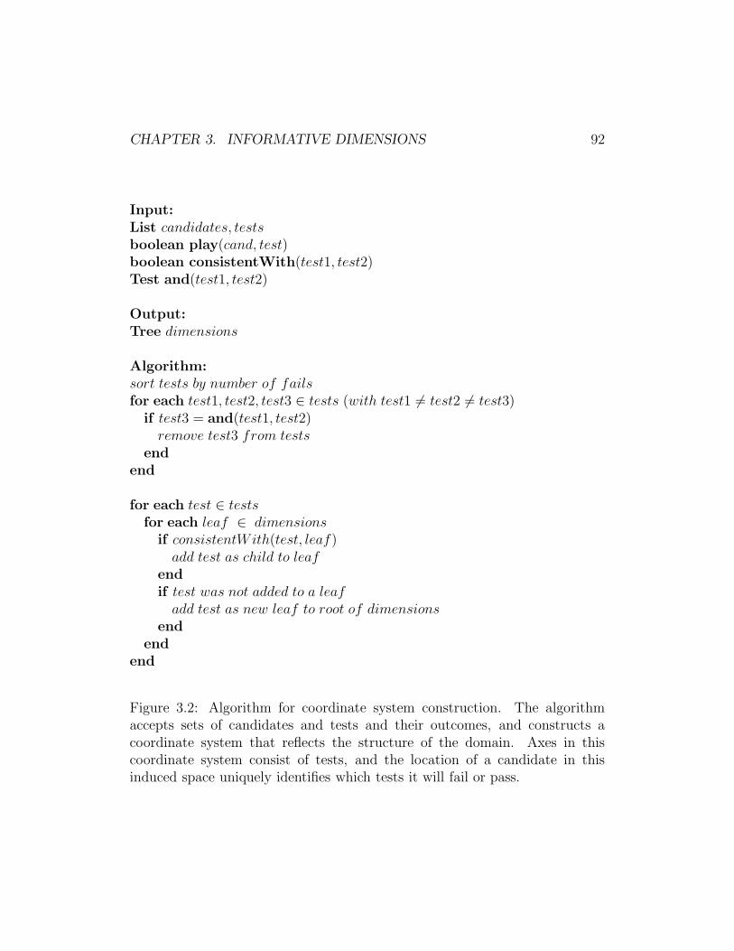
CHAPTER 3. INFORMATIVE DIMENSIONS 92
Input:List candidates, testsboolean play(cand, test)boolean consistentWith(test1, test2)Test and(test1, test2)
Output:Tree dimensions
Algorithm:sort tests by number of failsfor each test1, test2, test3 ∈ tests (with test1 6= test2 6= test3)
if test3 = and(test1, test2)remove test3 from tests
endend
for each test ∈ testsfor each leaf ∈ dimensions
if consistentWith(test, leaf)add test as child to leaf
endif test was not added to a leafadd test as new leaf to root of dimensions
endend
end
Figure 3.2: Algorithm for coordinate system construction. The algorithmaccepts sets of candidates and tests and their outcomes, and constructs acoordinate system that reflects the structure of the domain. Axes in thiscoordinate system consist of tests, and the location of a candidate in thisinduced space uniquely identifies which tests it will fail or pass.

CHAPTER 3. INFORMATIVE DIMENSIONS 93
2
4
6
8
10
12
14
16
2 4 6 8 10 12 14 16
Est
imat
ed n
umbe
r of
dim
ensi
ons
Number of dimensions
Estimated vs. actual number of dimensions, COMPARE-ON-ONE
2
4
6
8
10
12
14
16
18
20
1 2 3 4 5 6 7 8 9 10
Est
imat
ed n
umbe
r of
dim
ensi
ons
Number of dimensions
Estimated vs. actual number of dimensions, TRANSITIVE
Figure 3.3: Estimated number of dimensions in two numbers games, applyingthe algorithm in fig. 3.2 to the populations of a coevolutionary algorithm;see text for details. The left figure is the estimate for the Compare-on-
One game; note the tight correspondence with the theoretical number of di-mensions. On the right is the estimate for the Transitive game; here thealgorithm consistently overestimates.

Chapter 4
Emergent Geometric
Organization
4.1 Overview
This chapter argues the claim that algorithms augmented with an informa-
tiveness mechanism (or some equivalent) to dynamically select tests produce
better results than algorithms without such a mechanism. We argue the point
by giving two empirical studies, one comparing a Pareto coevolutionary al-
gorithm (P-PHC) against a more conventional coevolutionary algorithm on
two numbers games, the other comparing a cooperative coevolutionary algo-
rithm modified to use Pareto dominance (pCCEA) against a more conventional
CCEA. We observe
• That intransitivity in the domain does not necessarily lead to poor al-
94

CHAPTER 4. EMERGENT GEOMETRIC ORGANIZATION 95
gorithm performance, and that overspecialization is the more worrisome
pathology;
• That both intransitivity and overspecialization can be effectively ad-
dressed by comparing candidates using Pareto dominance and compar-
ing tests using informativeness (to allow dynamic selection of informative
tests);
• That the relative overspecialization phenomenon can also be effectively
addressed by comparing component parts using Pareto dominance, treat-
ing collaborators as tests.
We further observe in the numbers game experiments that when an in-
formativeness mechanism is in place, the population of test entities organizes
around the known dimensions in numbers game problems. This emergent ge-
ometric organization of the test entities in some sense corrals the candidate
solutions, preventing them from regressing on either dimension and thereby
avoiding overspecialization. It is unclear whether such an effect could be ex-
posed in the experiments on pCCEA, as there is no obvious way to visualize
the test domains in the plane. However, the improved performance of pC-
CEA over more conventional CCEAs suggests that something of the sort is
happening.
Section 4.2, an example of dynamic dimension selection, furthers the work
of chapter 3, section 3.2 by showing that any interactive domain represented
by a function of form p : S×T → R can be pseudoembedded into n-dimensional

CHAPTER 4. EMERGENT GEOMETRIC ORGANIZATION 96
Euclidean space for some n called the dimension of the domain. Based on that
observation, we can extend the observation made in chapter 3 that intransi-
tivity in the original domain disappears when Pareto dominance is used to
compare candidate entities. However, it is vital to realize that this conclusion
is only valid if we had all possible tests on hand to use for comparing. Since
a running algorithm never has such information available, this conclusion can
only be taken heuristically.
Nevertheless, the experiments in that section support the belief that this
heuristic conclusion can hold in practice. A Pareto coevolutionary algorithm,
P-PHC, which sues Pareto dominance to compare candidate entities and an
informativeness mechanism to compare tests does not have difficulties in the
intransitive domain pIG.
Imagining a domain embedded in an n-dimensional space suggests another
pathology, overspecialization. Ideally, we would like entities which have high
values on all dimensions of the domain. However, it may happen that instead
entities overspecialize on one dimension and neglect the others. A domain de-
signed to amplify this possibility, pFG is given. A conventional coevolutionary
algorithm, P-CHC, does indeed exhibit overspecialization behavior on this do-
main. However, P-PHC does not. Instead, P-PHC organizes the test entities
around the known dimensions of the domain, which pressures candidate enti-
ties to maintain capabilities on all dimensions simultaneously and thus avoid
overspecialization.

CHAPTER 4. EMERGENT GEOMETRIC ORGANIZATION 97
Section 4.3 reports the result of changing a conventional CCEA to com-
pare component parts using Pareto dominance over all possible collaborators.
The resulting algorithm, pCCEA, is compared to two other more conventional
CCEAs on two test problems designed to elicit the relative overgeneralization
phenomenon from CCEAs. The original, conventional CCEA exhibits this
phenomenon in every repetition of the experiment. cCCEA, a CCEA which
uses all possible collaborators for testing instead of just a subset, does not
exhibit relative overgeneralization on one test problem, but often exhibits it
on the second problem. pCCEA, by contrast, reliably avoids relative overgen-
eralization and finds the global optimum of both test problems.
Note that since cCCEA has access to all possible collaborators but uses the
maximum value to assign a part a single numerical fitness, cCCEA is subject to
the critiques of this practice raised in chapter 1. cCCEA has access to the same
pool of collaborators as pCCEA, yet pCCEA outperforms cCCEA on both test
problems. We conclude the switch away from using numerical fitnesses derived
from aggregates to using the multi-objective, Pareto dominance comparison
method explains the improved performance.
The results in this chapter are derived from previously published material.
Section 4.2 first appeared in [17], while section 4.3 is presented in [19].

CHAPTER 4. EMERGENT GEOMETRIC ORGANIZATION 98
4.2 Dynamic Dimension Selection and Under-
lying Objectives
This section extends the result of chapter 3, section 3.2 by showing that any
interactive domain represented by a function of form p : S × T → R can be
pseudoembedded into n-dimensional Euclidean space for some minimal n. We
conclude that intransitivity in the original domain disappears when Pareto
dominance is used to compare candidate entities. However, this conclusion is
only valid if we had all possible tests on hand to use for comparing. Since a
running algorithm never has such information available, this conclusion can
only be taken heuristically.
The experiments in that section support the belief that this heuristic con-
clusion can hold in practice. This section develops a Pareto coevolution al-
gorithm, P-PHC, which sues Pareto dominance to compare candidate entities
and an informativeness mechanism to compare tests does not have difficulties
in the intransitive game pIG.
Embedding a domain in an n-dimensional space suggests another pathol-
ogy, overspecialization. Ideally, we would like entities which have high values
on all dimensions of the domain. However, it may happen that entities over-
specialize on one dimension and neglect the others. A domain designed to
amplify this possibility, the focusing game pFG is given. We observe that
a conventional coevolutionary algorithm, P-CHC, does overspecialize in this
domain. However, P-PHC does not. Instead, P-PHC organizes the test enti-
CHAPTER 4. EMERGENT GEOMETRIC ORGANIZATION 99
ties around the known dimensions of the domain, which “corrals” candidate
entities to maintain capabilities on all dimensions simultaneously.
4.2.1 Orders and Coevolution
In this section we prove the preorder decomposition theorem. We apply our
results to interactive domains of form p : S × T → R, showing that any such
domain can be embedded into Euclidean n-space for some unknown n. Finally,
we work through an example to illustrate the concepts.
Applications to Coevolution
First, let us recall some important definitions and notation from chapter 2.
For any function f : S × T → R, where S is a set and R is a poset, write Sf
for the preordering induced on S by pullback, and write the order on Sf as
≤f . This definition means that s1 ≤f s2 exactly when f(s1) ≤R f(s2).1
As in definition 2.2.6, any function of form S × T → R can be curried to
a function of form S → [T → R], where [T → R] stands for the set of all
functions from T to R. If p : S × T → R, write λt.p for the corresponding
curried function.
Consequently, starting from an interactive domain p : S × T → R, with R
a poset, there is a corresponding preorder structure on the set S, namely the
Sλt.p we saw in definition 2.2.6. The basic idea is that two candidate solutions
1We can interpret this definition in terms of fitness functions: s1 ≤f s2 if s2’s fitness isat least as high as s1’s.

CHAPTER 4. EMERGENT GEOMETRIC ORGANIZATION 100
s1 and s2 lie in the relation s1 ≤λt.p s2 exactly when s2’s array of outcomes
covers s1’s. In other words, s2 does at least as well as s1 does against every
possible opponent. We refer the reader to chapter 3 for details and examples.
The poset decomposition theorem applies to partial orders, not preorders,
so we need to adjust it slightly. Our approach is to utilize the similarity relation
of definition 2.1.7. Recall that every preorder R comes with an equivalence
relation defined: s1 ∼ s2 if and only if s1 ≤R s2 and s2 ≤R s1. One way to
think about this relation is in the context of an objective function f : S → � .
s1 ∼ s2 exactly when the individuals s1 and s2 have the same fitness. In
a multi-objective context, s1 ∼ s2 when s1 and s2 have the same objective
vector. Given this equivalence relation, we can then prove the following:
Lemma 4.2.1. Let R be a finite preordered set. There is a canonical partially
ordered set Q = R/∼ and a surjective, monotone function π : R → Q (called
the projection) such that π(s1) = π(s2) if and only if s1 ∼ s2, for all s1, s2 ∈ R.
Q is called the quotient of R.
Proof. The proof that Q is a well-defined partial order is given in proposition
2.1.9. Let us show that π is surjective and monotone. Define π : R → Q by
π(s) = [s] for all s ∈ R, where [s] is the equivalence class of s under ∼. π is
surjective trivially, since the only equivalence classes in Q are of form [s] for
some s ∈ R. To see π is monotone, observe the order on Q is [s1] ≤Q [s2] if and
only if s1 ≤R s2. An equivalent way to state this definition is: π(s1) ≤Q π(s2)
if and only if s1 ≤R s2 (this is just rewriting [si] as π(si)). The “if” part proves

CHAPTER 4. EMERGENT GEOMETRIC ORGANIZATION 101
the monotonicity of π.
Lemma 4.2.1 permits us to adapt the poset decomposition theorem (the-
orem 2.3.5) to preorders. If R is a preorder, form the quotient Q = R/ ∼,
which will be a partial order. Apply the embedding lemma (lemma 2.3.7) to
yield an embedding φ : Q→�
n of Q in�
n . Composing φ with the projection
π gives a monotone function φ ◦ π : R →�
n which we call a pseudoembedding
of R into�
n . By this we mean the following. Write ψ for φ ◦ π. ψ is such
that ψ(s1) = ψ(s2) exactly when s1 ∼ s2. Consequently, ψ behaves like an
embedding, except that it sends equivalent individuals in R to the same point
in�
n . Otherwise, it sends non-equivalent elements in R to different points
in�
n while preserving the order relations between them. Let us record these
observations as:
Theorem 4.2.2 (Preorder Decomposition Theorem). Every finite pre-
order can be pseudo-embedded into�
n (and thus into � n). Moreover, every
finite preorder has a minimum n, the dimension of the preorder, for which
such pseudoembedding is possible.
Let us examine an example to help visualize the definitions.
Example 4.2.3. Consider the following game:.
p rock stone paper scissors
rock 0 0 −1 1
stone 0 0 −1 1
paper 1 1 0 −1
scissors −1 −1 1 0

CHAPTER 4. EMERGENT GEOMETRIC ORGANIZATION 102
paper
scissorsrock
stone
Figure 4.1: The preorder rock-stone-paper-scissors displayed as a graph. Anarrow between two individuals indicates a ≤ relationship; absence of an arrowindicates the individuals are incomparable.
This game is rock-paper-scissors with a clone of rock called “stone.” In
this case, S = T = {rock, stone, paper, scissors}, and R = {−1, 0, 1} with
−1 ≤ 0 ≤ 1.
By comparing the rows of this matrix, we can see that none of the strategies
dominates any of the others. Every strategy does well against at least one
opponent; likewise, every strategy does poorly against at least one opponent.
However, rock ∼ stone because their rows are identical. Consequently, the
induced preorder on {rock, stone, paper, scissors} contains only the relations
rock ≤ stone and stone ≤ rock. We show this preorder in figure 4.1.
When we mod out the equivalence relation ∼, we arrive at a partial order
consisting of the three equivalence classes {[rock], [paper], [scissors]}. In this
partial order, all three elements are incomparable to one another. This is, in
fact, a 2-dimensional partial order, with linear realizer L =
{([rock], [paper], [scissors]), ([scissors], [paper], [rock])}Figure 4.2 shows a plot
of the corresponding pseudoembedding.

CHAPTER 4. EMERGENT GEOMETRIC ORGANIZATION 103
0
1
2
3
4
5
0 1 2 3 4 5
Embedding of rock-stone-paper-scissors into Plane
[rock]={rock,stone}
[paper]={paper}
[scissors]={scissors}
Figure 4.2: The preorder rock-stone-paper-scissors pseudo-embedded into theplane
� 2
Discussion
We began with an interactive domain which may have had intransitive cycles
and other pathologies. We ended up with what amounts to an embedding of
the domain into�
n for some unknown dimension n.�
n is a particularly simple
partial order; in particular, it is transitive. How did we turn a pathological
problem into a nice transitive one?
The first point to note is that a pseudoembedding, while well-defined math-
ematically, is not easily computable. Indeed, it is has been known for some
time that even learning the dimension of a poset is NP-complete [110]. Fur-
thermore, to compute a poset decomposition, we need to have all the elements
of the poset on hand. While in many domains it is possible to enumerate all

CHAPTER 4. EMERGENT GEOMETRIC ORGANIZATION 104
solutions,2 it is typically intractable to do so. Thus, while pseudoembeddings
exist as mathematical objects, they are at least as expensive to compute as
solving the problem by brute force. This is not surprising; if we had a pseu-
doembedding in hand, we could treat our problem as a greater-than game
and solve it relatively easily. Pseudoembeddings thus encode a considerable
amount of information about the original domain which we have to “pay for”
somehow. In essence, what we have done is reorganize the information in a
domain.
A second point is that we can at least hope that the preorder decomposition
of an interactive domain can be approximated by a more practical algorithm.
In the next section, we will present a simple algorithm aimed at approximating
the preorder decomposition of a domain and show that it works reasonably
well on two instances of the numbers game.
4.2.2 Experiments
In this section we present our experimental results. We begin by recalling the
numbers game from [103]. Next, we describe the algorithms we employ and
our implementation choices. Finally, we present and discuss results.
The Numbers Game
“The numbers game” [103] actually refers to a class of games. Common among
them is that the set of individuals, call it S, consists of n-tuples of natural
2Exceptions include domains with real-valued parameters.

CHAPTER 4. EMERGENT GEOMETRIC ORGANIZATION 105
numbers. How we choose to compare individuals, and what choice we make for
n, define an instance of the game. In our experiments, we will be considering
two instances. In both, we will deviate somewhat from the score functions
defined in [103]. Instead of returning a score, we will construct our functions
to have form p : S × S → {0, 1}, where S =� 2 is the set of ordered pairs
of natural numbers, and the function p simply says which individual is bigger
(i.e., gets a bigger score or “wins” the game).
In our experiments we only present data for 2-dimensional domains, since
the issues we wish to emphasize are already visible at this low dimensionality.
For simplicity of presentation, we define these games for 2 dimensions only.
The Intransitive Game In this game, we first decide which dimensions of
the individuals are most closely matched, and then we decide which individual
is better on that dimension. The payoff function we use is:
pIG((i1, j1), (i2, j2)) =
1 if |i1 − i2| > |j1 − j2| and j1 > j2
1 if |j1 − j2| > |i1 − i2| and i1 > i2
0 otherwise
(4.1)
This game is intransitive; one cycle is (1, 6), (4, 5), (2, 4) [103]. (1, 6) and
(4, 5) are closest on the second dimension, so (1, 6) > (4, 5). (4, 5) and (2, 4)
are closest on the second dimension also, so (4, 5) > (2, 4). However, (2, 4) and
(1, 6) are closest on the first dimension, meaning (2, 4) > (1, 6). Nevertheless,
an individual with high values on both dimensions will tend to beat more

CHAPTER 4. EMERGENT GEOMETRIC ORGANIZATION 106
individuals than one without, and it seems, intuitively, that the best solutions
to this game are such individuals.
The Focusing Game In this game, the first and second individuals are
treated asymmetrically. The second individual is scanned to see on which
dimension it is highest. Then, it is compared to the first individual. The
first individual is better if it is higher on the best dimension of the second
individual. As a payoff function:
pFG((i1, j1), (i2, j2)) =
1 if i2 > j2 and i1 > i2
1 if j2 > i2 and j1 > j2
0 otherwise
(4.2)
Note that this game is transitive. However, the emphasis on one dimension
at the expense of others encourages individuals to race on one of the two
and neglect the second. Nevertheless, an individual which is high on both
dimensions will beat more individuals than one which is overspecialized on a
single dimension.
This game is closely related to the compare-on-one game described in
[35].3
3But note that pFG has range {0, 1} and requires strict inequalities for a 1 output,whereas compare-on-one has range {−1, 1} and does not require strict inequalities.
CHAPTER 4. EMERGENT GEOMETRIC ORGANIZATION 107
Algorithms and Setup
We will compare two algorithms, a population based coevolutionary hillclimber
(P-CHC) and a population based Pareto hillclimber (P-PHC). The P-CHC
has a single population. To assess the fitness of an individual, we sum how
it does against all other individuals according to the game we are testing.
The wrinkle is that each individual produces exactly one offspring, and the
offspring can only replace its parent if it is strictly better. This algorithm
uses a subjective fitness measure to assess individuals, but the constraint that
an offspring can only replace its own parent is a simple form of diversity
maintenance resembling deterministic crowding [63].
Our Pareto hillclimbing algorithm is similar in spirit to the DELPHI algo-
rithm presented in [35]. Our P-PHC operates as follows. There are two popu-
lations, candidates and tests. The candidates are assessed by playing against
all the tests. Rather than receiving a summed fitness, they receive an outcome
vector, as in evolutionary multi-objective optimization [48]. The outcome vec-
tors are then compared using Pareto dominance: candidate a is better than
candidate b if a does at least as well as b does versus all tests, and does better
against at least one. The tests are assessed differently, using an approximation
of informativeness. Since the outcome order is 0 < 1, the informativeness mea-
sure presented in section 3.2 collapses to comparing which pairs of candidates
a test says are equal. For our purposes, we will approximate informativeness
by simply counting how many pairs of candidates are made equal by a test.4 In
4This method has the advantage of being faster to compute. It is an approximation of

CHAPTER 4. EMERGENT GEOMETRIC ORGANIZATION 108
other words, each test has a score f(t) =∑
s1,s2∈Siδ(p(s1, t), p(s2, t)), where Si
is the current population, and δ(p(s1, t), p(s2, t)) returns 1 if p(s1, t) = p(s2, t),
0 otherwise. For our experiments, p will be one of pIG, or pFG. As in the co-
evolutionary hillclimber, in the Pareto hillclimber individuals receive only one
offspring, and an offspring can only replace its parent. However, the climbing
is done separately in the two populations.5
To factor out issues of representation and focus on evaluation, in our ex-
periments, genotype=phenotype. That is, individuals are simply pairs of num-
bers. To create a mutant, we add random noise to each coordinate with some
probability. Notice there is no mutation bias in any particular direction.
We will be using a population size of 100 for all experiments. In the
coevolutionary hillclimber, the single population will be 100 individuals; in
the Pareto hillclimber, there will be 50 candidates and 50 tests. The mutation
rate is 100%; mutation adds +1 or -1 to each dimension. No form of crossover
is used. We ran each simulation for 500 time steps.
Results
Figures 4.3 and 4.4 show performance versus evolutionary time for both P-CHC
and P-PHC on the payoff functions pIG and pFG. Note that the coevolutionary
hillclimber out paces the Pareto hillclimber. The Pareto hillclimber must
informativeness in the sense that two tests which receive unequal counts are incomparableaccording to the informativeness order.
5We should remark that neither of these algorithms was intended to be practical; rather,they are intended to test our ideas.

CHAPTER 4. EMERGENT GEOMETRIC ORGANIZATION 109
0
50
100
150
200
250
300
350
400
0 50 100 150 200 250 300 350 400 450 500
Per
form
ance
(su
m o
f coo
rds)
Evolutionary time
Performance of P-CHC and P-PHC on IG, versus Time
P-CHCP-PHC
Figure 4.3: Performance versus time of P-CHC and P-PHC on IG (intransitivegame). Plot shows a single, typical run. Performance is measured as the sumof the coordinates; the plot shows this value for the best individual of thepopulation at each time step.
adjust not only its candidates to make an improvement, but also its tests.
Updating the tests causes a lag, which slows down progress. The graphs are
intended to be qualitative, however; what is important is that both algorithms
make steady progress.
Note figure 4.3, the intransitive game. Unlike the algorithm used in [103],
P-CHC made continuous progress on the intransitive game. Since P-CHC
essentially adds only a diversity maintenance mechanism, it seems the diversity
is important to the success or failure of coevolution on this domain.
At first glance, the Pareto coevolution mechanism of P-PHC does not seem
to be adding anything. To understand more completely what is happening, in
figure 4.5, we plot the final candidates P-CHC found on a typical run on pFG,

CHAPTER 4. EMERGENT GEOMETRIC ORGANIZATION 110
0
50
100
150
200
250
300
350
400
0 50 100 150 200 250 300 350 400 450 500
Per
form
ance
(su
m o
f coo
rds)
Evolutionary time
Performance of P-CHC and P-PHC on FG, versus Time
P-CHCP-PHC
Figure 4.4: Performance of P-CHC and P-PHC on FG (focusing game). Plotshows a single, typical run. Performance is measured as the sum of the coor-dinates of the best individual.
together with the final candidates and tests which P-PHC found on a typical
run. Notice how P-CHC has overspecialized entirely on the horizontal dimen-
sion. While it made great progress there, it neglected the vertical dimension
entirely. By contrast, P-PHC has maintained progress on both dimensions
equally. While it did not move as far as P-CHC, it did remain balanced. Most
important are the tests P-PHC found. In the plot, the tests appear to be “cor-
ralling” the candidates, keeping them in a tight group near the main diagonal.
An animation of a typical run of P-PHC reveals this is indeed the case. The
tests keep step behind the candidates. The same configuration of tests and
candidates persists, but the group of them move slowly up and to the right,
towards the better values of this game.
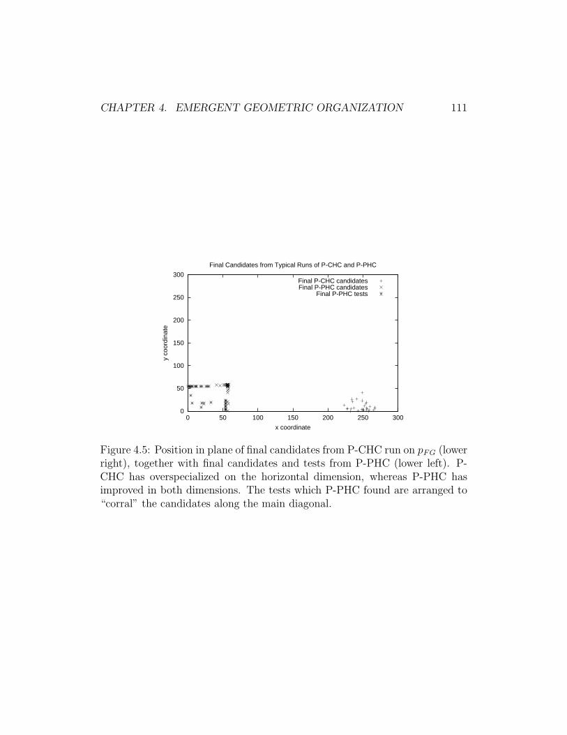
CHAPTER 4. EMERGENT GEOMETRIC ORGANIZATION 111
0
50
100
150
200
250
300
0 50 100 150 200 250 300
y co
ordi
nate
x coordinate
Final Candidates from Typical Runs of P-CHC and P-PHC
Final P-CHC candidatesFinal P-PHC candidates
Final P-PHC tests
Figure 4.5: Position in plane of final candidates from P-CHC run on pFG (lowerright), together with final candidates and tests from P-PHC (lower left). P-CHC has overspecialized on the horizontal dimension, whereas P-PHC hasimproved in both dimensions. The tests which P-PHC found are arranged to“corral” the candidates along the main diagonal.
CHAPTER 4. EMERGENT GEOMETRIC ORGANIZATION 112
4.2.3 Discussion
To sum up, we have shown mathematically that a wide class of interactive do-
mains, if properly construed, can be looked upon as n-dimensional, transitive,
greater-than games. The trouble is that discovering n is an NP-complete prob-
lem in general, let alone the embedding which would permit us to convert our
favorite interactive domain to a nicely-behaved transitive domain. Neverthe-
less, we feel the mathematical result does change the face of intransitivity. We
examined intransitivity experimentally, using insights gained from the math-
ematics, and saw that it may not be the demon it has been made out to be.
Instead, it may be that algorithms fail because they are overspecializing on
some dimensions of a domain at the expense of others.
4.3 Dynamic Dimension Selection and Rela-
tive Overgeneralization
This section reports the result of augmenting a conventional CCEA with a
Pareto dominance comparison of candidates, where dominance is taken over all
possible collaborators. The resulting algorithm, pCCEA, is compared to two
other, more conventional CCEAs on two maximum of two quadratics (MTQ)
problems designed to amplify relative overgeneralization. These problems have
two critical points, one of which is a local optimum sitting on a low, wide peak,
the other of which is a global optimum sitting on a wide, narrow peak. Relative
CHAPTER 4. EMERGENT GEOMETRIC ORGANIZATION 113
overgeneralization leads algorithms to prefer the lower, wider peak. In fact,
an analysis of the MTQ domains reveals that the initial population of the
algorithm is very likely to contain representatives on the peak containing the
global optimum. Yet the CCEA and cCCEA algorithms often do not find this
optimum, suggesting they actively pull away from the higher peak. Thus, the
relative overgeneralization phenomenon is not an accident of noise or drift, but
is encouraged by the selection method used in the algorithm.
Empirically, we observe that the original, conventional CCEA exhibits this
phenomenon in every repetition of the experiment. cCCEA, a CCEA which
uses all possible collaborators for testing instead of just a subset, does not
exhibit relative overgeneralization on one test problem, but often exhibits it
on the second problem. pCCEA, by contrast, reliably avoids relative overgen-
eralization and finds the global optimum of both test problems.
Note that since cCCEA has access to all possible collaborators but uses the
maximum value to assign a part a single numerical fitness, cCCEA is subject to
the critiques of this practice raised in chapter 1. cCCEA has access to the same
pool of collaborators as pCCEA, yet pCCEA outperforms cCCEA on both test
problems. We conclude the switch from numerical fitnesses from aggregates
to the multi-objective, Pareto dominance comparison method explains the
improved performance.
This section is organized as follows. In section 4.3.1 we give necessary
background from Pareto coevolution and cooperative coevolution. In section
4.3.2 we give and analyze the particular Maximum of Two Quadratics used

CHAPTER 4. EMERGENT GEOMETRIC ORGANIZATION 114
in [78] and in the experiments reported here. In section 4.3.3 we present our
experimental results. Finally, in section 4.3.4 we discuss implications of what
we have observed.
4.3.1 Background
Pareto Coevolution
Much of the material we are reviewing here can be found in more detail in
chapter 3, which should be consulted for details.
Let p : S × T → R be a function; here S and T are sets and R is a
preordered set. The set S can be thought of as the set of candidate solutions
(candidates). These are the entities which an algorithm is meant to optimize.
The set T can be thought of as tests; these individuals serve to test or measure
the candidates and give information about how good they are. The ordered set
R can be thought of as results or outcomes of interactions between candidates
and tests.
It is worth pointing out that both candidates and tests are roles that in-
dividuals can take. When we have an algorithm like a CCEA over a function
f : X × Y → � , we are in much the same situation as above: a two-place
function into an ordered set. However, the situation is slightly different. The
CCEA aims to optimize both individuals in X and individuals in Y ; thus these
sets act variously as candidates and tests. At the stage of the algorithm when
X elements are selected, X is acting as the candidate set to be optimized; the

CHAPTER 4. EMERGENT GEOMETRIC ORGANIZATION 115
possible collaborators from Y can then be thought of as tests measuring the
X values. However, when we consider updating Y , the roles reverse: the Y
values are candidates and the X values are tests.
Let us return to the function p. We can use this function to compare two
candidates s1, s2 ∈ S as follows: s2 (Pareto) covers s1, which we will denote
s1 � s2 if, for all t ∈ T , p(s1, t) ≤ p(s2, t). If each t ∈ T is thought of as
a test, this relation says that for each test, s2 does at least as well as s1. s2
Pareto dominates s1 if s1 � s2 and, in addition, there is a t ∈ T such that
p(s1, t) < p(s2, t). That is, s2 is at least as good as s1 against all tests and is
strictly better than s1 against at least one test.
If it happens that there are t1, t2 ∈ T such that p(s1, t1) < p(s2, t1) but
p(s1, t2) > p(s2, t2), then s1 and s2 are incomparable. We will denote incom-
parability s1 � s2 as in definition 2.1.5. The idea of incomparability in this
instance is that there are two tests, one which shows s2 is better than s1,
but another which shows s1 is better than s2. In this case we cannot give a
strict relationship between the two candidates; they each have value, albeit in
different ways.
The relation � is a preorder on the set S. As such it has a set of maximal
elements; these are elements s ∈ S such that if s � s, then s � s must also
hold, for any s ∈ S. In words, s is maximal if, whenever it appears to be
less than or equal to some other value, that value is less than or equal to it
(meaning the two values are equivalent). The set of all maximal elements of
� is called the Pareto optimal set, Pareto front, or non-dominated front by

CHAPTER 4. EMERGENT GEOMETRIC ORGANIZATION 116
various authors.
Thus far we have considered comparing candidates in S. What about the
tests in T ? An observation made in [42] is that it is not appropriate to use
Pareto covering or Pareto dominance to compare tests. Rather, as advocated
there and indeed in this dissertation as a whole, it makes sense to compare tests
according to how informative they are about ranking candidates. It suffices for
our purposes to consider two cases. If two tests t1, t2 ∈ T rank all the candidate
individuals in the same order, then they are equally informative. However, if
there are s1, s2 ∈ S such that p(s1, t1) < p(s2, t1) and p(s1, t2) > p(s2, t2), then
the tests t1 and t2 are differently informative.
Cooperative Coevolution
Cooperative coevolution has generally been presented as a framework as op-
posed to a particular algorithm. We will follow the scheme given in algorithm
2 of [105]. The algorithm keeps some indexed set of populations ps. For each
population ps, parents are selected, offspring generated via the variation op-
erators, collaborators are selected from the remaining populations, and the
individuals of ps are evaluated with these collaborators. The next generation
for population ps consists of the individuals which survive selection based on
this evaluation. Within this framework one is free to use whichever selection,
generation, variation, collaboration, and evaluation mechanism one wishes. In
what follows we will detail the choices which were made for the experiments
reported in section 4.3.3.

CHAPTER 4. EMERGENT GEOMETRIC ORGANIZATION 117
Some applications of cooperative coevolution involve a function of form
f : X×Y → � . The task is to find values in the sets X and Y which optimize
this function. One way to approach optimizing such a function is to define
two populations corresponding to settings for X and Y . The evaluation of two
individuals x ∈ X and y ∈ Y can then be f(x, y) or some function thereof.
Relative overgeneralization is already evident in simple scenarios like this one.
We will be considering two Maximum of Two Quadratics (MTQ) functions
[105]. Let f1 and f2 be two quadratic functions defined:
f1(x, y) = h1
(1 −
16(x− x1)2
s1−
16(y − y1)2
s1
)
f2(x, y) = h2
(1 −
16(x− x2)2
s2
−16(y − y2)
2
s2
)
where hi, si, xi and yi are parameters controlling the height, width, and
vertex of the function. Given two such functions, an MTQ function is defined:
MTQ(x, y) = max(f1(x, y), f2(x, y)) (4.3)
The function employed in [78] uses the following parameter settings: h1 =
50, s1 = 1.6, (x1, y1) = (34, 3
4); and h2 = 150, s2 = 1
32, (x2, y2) = (1
4, 1
4). 6 We
will denote this function MTQ1. We will also be considering a second function
MTQ2 which is MTQ1 but with h1 = 125. These two functions are displayed
6We have switched the positions of the global and local optima versus what was reportedin Panait et al.

CHAPTER 4. EMERGENT GEOMETRIC ORGANIZATION 118
00.2
0.40.6
0.81 0
0.20.4
0.60.8
1−500−400−300−200−100
0100200
Figure 4.6: Plot of MTQ1.
00.2
0.40.6
0.81 0
0.20.4
0.60.8
1−1400−1200−1000−800−600−400−200
0200
Figure 4.7: Plot of MTQ2.
in Figs. 4.6 and 4.7.
In our experiments we will be comparing three CCEAs. The first is as
in [78]; for brevity we call this algorithm simply CCEA. The sets X and Y
are both sets of reals, the unit interval [0, 1]. There are two populations,
one consisting of 32 individuals from X, the other containing 32 individuals
from Y . Tournament selection is used. Here, to perform selection on X for
example, two individuals x1, x2 are selected at random from the X popula-
tion. These individuals are varied by adding Gaussian noise with mean 0 and
standard deviation 0.05. Then the individuals are evaluated. Evaluation is
done by selecting the highest-valued individual y∗ from the Y population of

CHAPTER 4. EMERGENT GEOMETRIC ORGANIZATION 119
the previous generation7 as well as a random individual y. x1’s evaluation is
max(MTQ(x1, y∗),MTQ(x1, y)); i.e., the objective function value of x1 and
its best collaborator. Once evaluation is performed, a random value r between
0 and 1 is chosen. If r ≤ k, then the higher-valued of x1, x2 is added to the
next population; otherwise the lower-valued individual is added. Here k is
a parameter controlling the selection pressure; we have used k = 0.75 in all
experiments reported. One last point is that the highest-valued individual
of the previous generation is always carried forward unmodified to the next
generation.
The second CCEA variant, which we call pCCEA, has two modifications
over CCEA. First, at the stage when individuals are being compared, objective
value with a collaborator is not used. Instead, the two individuals are com-
pared according to Pareto dominance. That is, instead of considering adding
the individual with the higher objective value, we consider adding the domi-
nant individual; for instance, if x1 � x2 and r ≤ k, then x2 is added to the
next generation. If x1 � x2, both are added to the next generation. Second,
since there is no notion of best individual in this case, we will carry forward the
non-dominated front of the previous generation. It is possible that dominated
individuals make it into the population; thus, we first find the Pareto front of
the current population, carry that forward to the next generation, and fill in
any remaining space in the population with individuals selected as above.
The final CCEA, which we call cCCEA, has one modification over CCEA.
7Or from the current generation at step 1 of the algorithm

CHAPTER 4. EMERGENT GEOMETRIC ORGANIZATION 120
Instead of comparing individuals according to the best setting of the previous
generation, we will have each individual collaborate with all individuals in
the other population and give it the highest value it receives from all these
collaborations. We will use cCCEA as a control for pCCEA: since the Pareto
dominance mechanism in pCCEA has access to all individuals in the test
population, it seems only fair to give CCEA the same information and see
how well it performs.
4.3.2 Analysis
In this section we make two observations:
1. The initial populations of 32 X and Y settings frequently represent indi-
viduals on the higher peak. That is, there is a setting in the X population
and a setting in the Y population which, when paired together, lie on
the higher-valued peak;
2. In the domain defined byMTQ1, the globally-optimal and locally-optimal
settings for one population are Pareto optimal as well as being differently
informative when treated as tests of the other population.
The import of the first observation is that the initial population of these
algorithms already contains individuals which could potentially move to the
global optimum. In the case of the CCEA without the Pareto dominance
mechanism, the experimental observation that the algorithm often does not

CHAPTER 4. EMERGENT GEOMETRIC ORGANIZATION 121
find this global optimum implies that the algorithm is actively moving away
from the higher-valued peak.
The import of the second observation is that, unlike the situation in com-
petitive domains, a CCEA running on these MTQ functions does not require
an explicit informativeness mechanism to keep informative tests in the popu-
lation. Pareto dominance suffices. The reason is that in competitive domains,
Pareto dominant individuals tend to make poor tests; thus there is a need for
a separate mechanism to encourage informative tests to remain in the popu-
lation. In MTQ1 at least, the situation is different: Pareto optimal settings
tend to also be informative tests of their collaborators.
Initial Populations and the Higher Peak
We will show that, with an initial population of 32 X and Y individuals,
the initial population of a CCEA has roughly a 90% chance of containing a
representative on the higher-valued peak. To prove this, we will show that all
points (x, y) in the square spanned by the points (0.2, 0.2) and (0.29, 0.29) are
such that f2(x, y) > f1(x, y); i.e. are such that MTQ1(x, y) = f2(x, y). As
a result, the points are within this square are all on the higher-valued peak.
We will then calculate the probability that the initial population contains at
least one point in this square; this probability will give a lower bound on the
probability that the population contains a representative on this peak.
Because the region for which this relation holds is simply connected, it
suffices to show the corners of the square are all such that f2(x, y) > f1(x, y).

CHAPTER 4. EMERGENT GEOMETRIC ORGANIZATION 122
(x, y) f1 f2
(0.2, 0.2) -252.5 -225.0(0.2, 0.29) -207.05 -157.5(0.29, 0.2) -207.05 -157.5(0.29, 0.29) -161.6 -90.0
Table 4.1: Values of f1 and f2 on four points in the xy-plane spanning a squarewhich lies under the higher-valued peak.
In table 4.1 we give the values of f1 and f2 for the four corners of this square;
for all four points f2’s value is larger.
The probability that a value chosen uniformly randomly in the range [0, 1]
will land in the subinterval [0.2, 0.29] is p = 0.09. Now, if 32 values are
chosen uniformly randomly, the chance that at least one of them will lie in
the subinterval is 1 − (1 − p)32 or approximately 0.95. In other words, the
chance that the initial population of X values has at least one individual in
this range is roughly 0.95; similarly for Y . Thus, the probability that the initial
population has at least one X value and one Y value in [0.2, 0.29] is roughly
0.95·0.95 or roughly 0.90. In short, roughly 90% of runs of a CCEA with initial
population of 32 X and Y values should have at least one representative on
the higher-fitness peak.
Dominance and Informativeness
Much can be said about the dominance and informativeness structure in the
domain defined by MTQ1. We will simply show that the globally- and locally-
optimal individuals are Pareto optimal when treated as candidates and differ-

CHAPTER 4. EMERGENT GEOMETRIC ORGANIZATION 123
ently informative when treated as tests. Note that because of the symmetry
of the MTQ1 function, all statements made treating X individuals as candi-
dates apply equally well when Y values are treated as candidates. Similarly,
statements about Y individuals as tests apply when X individuals are treated
as tests.
Regarding dominance, let the Y values be candidates and X values tests.
Let y∗ = 14
be the globally-optimal setting for Y and let y∗ = 34
be the locally-
optimal setting. Fig. 4.8 depicts these two candidates as functions of X.
Note they are incomparable. For x1 ∈ (x, x′), MTQ1(x1, y∗) < MTQ1(x1, y∗).
However, for x2 6∈ [x, x′], MTQ1(x2, y∗) > MTQ1(x2, y∗). Thus, there is a
test, x1 which says that y∗ is better than y∗ and a test x2 which says that y∗
is better than y∗.
Furthermore, both these settings are Pareto optimal. For y∗, note that the
corresponding x∗ is such that for all y ∈ Y , MTQ1(x∗, y) < MTQ1(x∗, y∗).
Consequently, y∗ cannot be dominated and so must lie on the Pareto front.
Similarly, for y∗, MTQ1(x∗, y) < MTQ1(x
∗, y∗), meaning y∗ cannot be domi-
nated. Therefore both y∗ and y∗ are Pareto optimal as candidates.
Now let us consider informativeness when treating Y settings as tests.
Partition Y into two subsets T1 and T2 as follows: T1 = {y ∈ T |∀x ∈
X,MTQ1(x, y) = f1(x, y)} and T2 = Y \ T1. Note that y∗ ∈ T1 (because
all points (x, y∗) are on the lower-valued peak; see fig 4.8) and y∗ ∈ T2.
First we observe that all tests in T1 are equally informative. Recall that
this means they all put the X settings in the same order. Let y, y ′ ∈ T1 and

CHAPTER 4. EMERGENT GEOMETRIC ORGANIZATION 124
y*
y*
(x,x’)
−400
−300
−200
−100
0
100
200
0 0.2 0.4 0.6 0.8 1
Figure 4.8: Plot of candidates y∗ and y∗ as cross sections through MTQ1.The shaded interval (x, x′) consists of those X settings for which y∗ is betterthan y∗; for the remaining X settings, y∗ is better than y∗, making the twonon-dominated.
define two functions on X:
g(x) = f1(x, y)
h(x) = f1(x, y′)
Simply, g gives the value of x ∈ X when y is applied to it; h gives the value
of x when y′ is applied. Now let x, x′ ∈ X. Then g(x) ≤ g(x′) if and only if
h(x) ≤ h(x′). To see this, notice that g(x)+h116(y−y1)2
s1
−h116(y′−y1)2
s1
= h(x) for
any x. Since adding a quantity to both sides of an inequality does not change
its direction, g(x) ≤ g(x′) implies h(x) ≤ h(x′). A symmetrical argument
shows that h(x) ≤ h(x′) implies g(x) ≤ g(x′). Therefore g and h both induce
the same order on X by pullback. Since g(x) = f1(x, y) = MTQ1(x, y) and
h(x) = f1(x, y′) = MTQ1(x, y
′), it follows that y and y′ order X in the same
way. In other words y and y′ are equally informative tests. In particular, since
y∗ ∈ T1, this test orders X in the same way as all other tests in T1.

CHAPTER 4. EMERGENT GEOMETRIC ORGANIZATION 125
y=0.5
xx*
y’=0.25
−400
−300
−200
−100
0
100
200
0 0.2 0.4 0.6 0.8 1
Figure 4.9: Cross sections through MTQ1 defined by two different Y values.x∗ and x depicted here satisfy relations 4.4 through 4.6.
The situation in T2 is more complicated than in T1. It is beyond our scope
to go into a detailed analysis of the informativeness structure for T2. However,
we observe that the tests in T2 are differently informative than those in T1. To
see this, let y ∈ T1 and y′ ∈ T2, let x∗ = 14
be the globally-optimal X setting
and let x ∈ X be such that:
f1(x∗, y) < f1(x, y) (4.4)
f2(x, y′) < f1(x, y
′) (4.5)
f1(x, y′) < f2(x
∗, y′) (4.6)
Fig. 4.9 illustrates these relationships.
Relation 4.4 implies that MTQ1(x∗, y) < MTQ1(x, y), in other words that
test y ranks x∗ strictly lower than x. Relation 4.5 implies that MTQ1(x, y′) =
f1(x, y′). By definition of x∗, MTQ1(x
∗, y′) = f2(x∗, y′). Thus, relation 4.6
implies that MTQ1(x, y′) < MTQ1(x
∗, y′) or, in other words, that test y′
ranks x∗ strictly higher than x. In short, the tests y and y′ rank x and x∗

CHAPTER 4. EMERGENT GEOMETRIC ORGANIZATION 126
differently, so are differently informative. y and y′ were chosen arbitrarily from
T1 and T2, respectively, meaning that any test in T1 is differently informative
from any other test in T2. In particular, y∗ and y∗ are differently informative.
Recall that these two settings are also Pareto optimal; therefore we have shown
that two Pareto optimal settings for Y also make differently informative tests,
indicating a close relationship between Pareto dominance and informativeness
which is not typically present in competitive domains.
4.3.3 Experiments
In this section we will report on the experiments performed. We replicate the
case reported in [78] on MTQ1 when δ = 0. We then perform the same exper-
iment, this time using Pareto dominance to compare individuals as outlined
in section 4.3.1.
We ran CCEA, pCCEA, and cCCEA for 50 generations on MTQ1. We
repeated this experiment 250 times for each algorithm. Table 4.2 reports the
number of runs which found an individual near the global optimum8 and gives
the mean objective value of the highest-valued individual from each of the
250 runs. Recall that the objective value of the higher peak is 150, while
the objective value of the lower peak is 50. CCEA never finds high-quality
individuals; instead it always finds individuals at or near the local optimum,
corroborating what was observed in [78] (see, for instance, Fig. 2 in that paper
for the case δ = 0). By contrast, pCCEA reliably finds individuals at or near
8By which we mean the X and Y settings are in the range [0.24, 0.26]
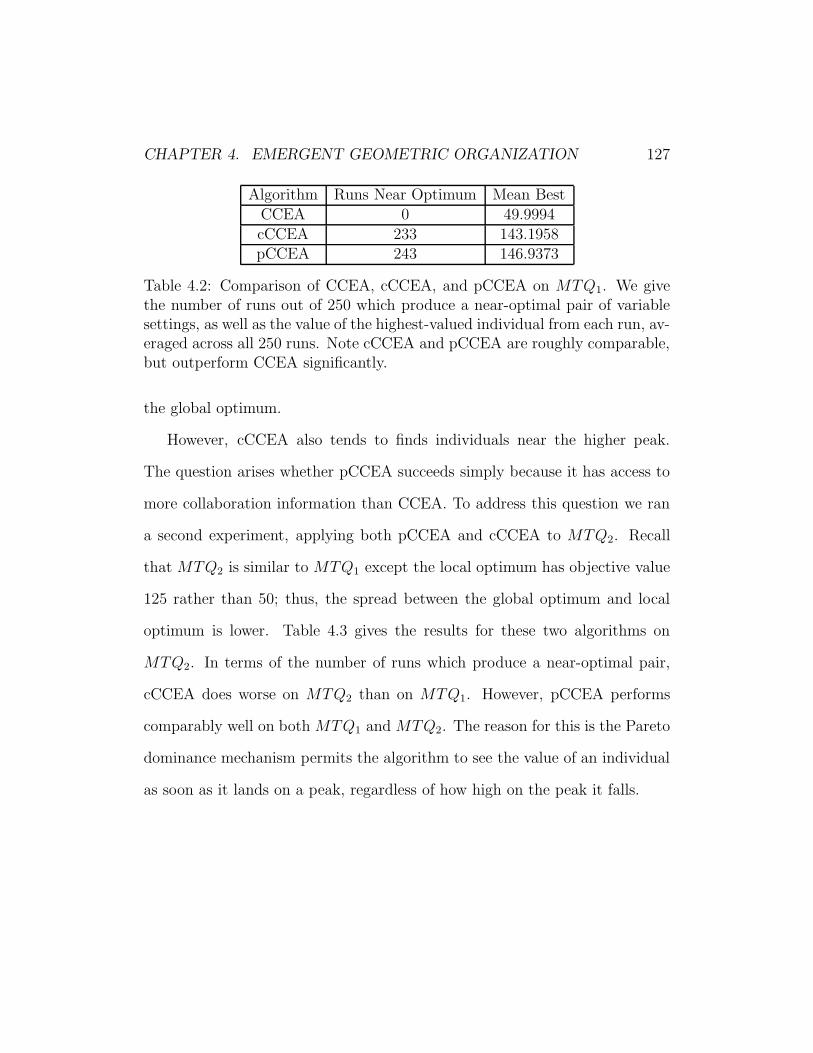
CHAPTER 4. EMERGENT GEOMETRIC ORGANIZATION 127
Algorithm Runs Near Optimum Mean BestCCEA 0 49.9994cCCEA 233 143.1958pCCEA 243 146.9373
Table 4.2: Comparison of CCEA, cCCEA, and pCCEA on MTQ1. We givethe number of runs out of 250 which produce a near-optimal pair of variablesettings, as well as the value of the highest-valued individual from each run, av-eraged across all 250 runs. Note cCCEA and pCCEA are roughly comparable,but outperform CCEA significantly.
the global optimum.
However, cCCEA also tends to finds individuals near the higher peak.
The question arises whether pCCEA succeeds simply because it has access to
more collaboration information than CCEA. To address this question we ran
a second experiment, applying both pCCEA and cCCEA to MTQ2. Recall
that MTQ2 is similar to MTQ1 except the local optimum has objective value
125 rather than 50; thus, the spread between the global optimum and local
optimum is lower. Table 4.3 gives the results for these two algorithms on
MTQ2. In terms of the number of runs which produce a near-optimal pair,
cCCEA does worse on MTQ2 than on MTQ1. However, pCCEA performs
comparably well on both MTQ1 and MTQ2. The reason for this is the Pareto
dominance mechanism permits the algorithm to see the value of an individual
as soon as it lands on a peak, regardless of how high on the peak it falls.

CHAPTER 4. EMERGENT GEOMETRIC ORGANIZATION 128
Algorithm Runs Near Optimum Mean BestcCCEA 177 142.6876pCCEA 248 149.3980
Table 4.3: Control experiment comparing cCCEA and pCCEA on MTQ2. Wegive number of runs out of 250 which produce a near-optimal pair of variablesettings, as well as the value of the highest-valued individual from each run,averaged across all 250 runs. Note cCCEA performs significantly worse on thisproblem than on MTQ1, whereas pCCEA performs comparably well.
4.3.4 Discussion
We began with the question of modifying the CCEA to promote the discov-
ery of global optima. pCCEA, a cooperative coevolutionary algorithm using
a Pareto dominance mechanism to compare individuals, achieves this aim re-
markably well. When compared with CCEA, pCCEA performs quite a bit
better. When compared with another modification of CCEA which uses the
same number of evaluations per generation against the same pool of collab-
orators (cCCEA), pCCEA performs comparably on MTQ1 but significantly
better on MTQ2. The explanation we give for the difference in performance on
MTQ2 is that cCCEA is sensitive to the relative, numerical objective values
of the two peaks, whereas pCCEA is sensitive to informational differences be-
tween individuals and is insensitive to their numerical values. One might say
that while maximizing performance over all collaborators shows how different
A is from B, Pareto dominance reveals how A is different from B. pCCEA’s
ability to find global optima suggests ideas from Pareto coevolution may fruit-
fully be applied to optimization with CCEAs in other domains, and supports

CHAPTER 4. EMERGENT GEOMETRIC ORGANIZATION 129
the critique of using aggregate fitness measures raised in chapter 1.
4.4 Discussion
Section 4.2 argued that any interactive domain expressed with a function of
form p : S × T → R can be construed as a greater-than game in some n-
dimensional Euclidean space. Such games would be straightforward for even
the simplest algorithms (provided n is small enough), if only the embedding
were known. Of course, such an embedding is exactly what is not known in
advance; in fact, it is not unreasonable to say that a successful coevolutionary
algorithm develops at least some part of such an embedding while running.
The organization of the test entities around the dimensions of the pFG do-
main is remarkable in that neither the game nor the algorithm exposes this
information. Rather, it is revealed or emerges as a consequence of the dynam-
ics induced by the informativeness mechanism. A very similar observation
has been made with a different algorithm, DELPHI, which uses a discrimina-
tion mechanism similar to informativeness to incent test entities [35]. These
observations suggest that emergent geometric organization may be a robust
phenomenon.
Section 4.3 did not directly treat the question of emergent geometric orga-
nization because the MTQ test functions used cannot easily be analyzed and
visualized to reveal the effect. However, the improvement of performance of
pCCEA over cCCEA and CCEA suggests that such an effect is occurring. The

CHAPTER 4. EMERGENT GEOMETRIC ORGANIZATION 130
collaborator pool used to test component parts must be maintaining a kind of
informational diversity to allow pCCEA to identify and scale the higher peak,
as the algorithms which do not have this mechanism fail to do so. Juxtapos-
ing these results on relative overgeneralization with those on overspecialization
suggest that the two phenomena may be closely linked and only appear differ-
ent because of the differences between the domains explored by the algorithms.
That is, adversarial domains which aim to evolve capable candidates may ex-
pose different algorithm misbehavior from cooperative domains which aim to
evolve capable wholes build from all types of entity, when at the core the
misbehavior is always arising from a failure to test adequately. The fact that
an informativeness criterion alleviates both pathologies is suggestive in this
regard.
Not to put too fine a point on it, section 4.3.2 showed that on MTQ1,
informativeness and Pareto optimality coincide to some degree: certain Pareto
optimal individuals are also differently informative. This observation raises an
intriguing question: could the relationship between informativeness and Pareto
dominance yield a metric of how competitive or cooperative a domain is? It
has been observed previously that in domains which have traditionally been
called competitive, for instance game playing, This dissertation has argued
that performing and informing, here Pareto dominance and informativeness,
are different: highly capable, dominant players are poor tests. In the domain
of chess playing, for example, Garry Kasparov is a dominant player, but the
outcomes of a set of players’ games against Kasparov would yield very little

CHAPTER 4. EMERGENT GEOMETRIC ORGANIZATION 131
information about how the players compare to one another. In short, the
discrepancy between informativeness and dominance in competitive domains
is marked, whereas at least on these examples of cooperative domains, the two
concepts appear related.

Chapter 5
Conclusions, Critiques and
Corollaries
Chapter 1 argued for a reassessment of the arms race conception of com-
petitive coevolutionary algorithms. Several pathological algorithm behaviors
which forestall arms races, particularly overspecialization and cycling, were
considered from the perspective of how entities were measured. In particular,
a conceptual split was drawn between performance, the measurement of how
well an entity performs at the task, and informativeness, the measurement
of how well an entity informs about the performance of other entities. The
reliance of previous methods on a single, numerical fitness value derived from
interactions with entities which were only incented to perform was posited as
the primary culprit in producing pathological algorithm behavior and prevent-
ing arms races from arising.
132
CHAPTER 5. CONCLUSIONS, CRITIQUES AND COROLLARIES 133
The chapter continued by arguing that cooperative coevolutionary algo-
rithms are vulnerable to the same critique. Though these algorithms have not
historically been conceived of as attempting to create and sustain arms races,
they do assess entities, or component parts, with collaborators drawn from a
pool of entities which have only been incented to perform. They also aggregate
interaction information into a numerical fitness assessment, just as competi-
tive coevolutionary algorithms do. Thus, they rely on the same questionable
basis of measurement that prevents arms races in competitive coevolutionary
algorithms. Seen in this light, the ongoing debate over collaboration selec-
tion methods, as well as the relative overgeneralization phenomenon, may also
stem from the shortcomings of numerical, aggregate measurements coming
from interaction with entities incented to perform.
In short, the difficulties encountered when applying either competitive or
cooperative coevolutionary algorithms were argued to arise from a common
cause: a failure of measurement, and in particular a failure to adequately and
explicitly treat the adaptation of the function of measurement in troubled
algorithms.
Given that single, aggregated fitness values are suspect, the question of
what to do instead arises. The case was made that switching to a multi-
objective value system is both possible and useful. Furthermore, if the cal-
culation of fitness from interactions with entities which were only incented to
perform is also troublesome, what can be done about that? The answer lay
in designing algorithms which explicitly incent entities to inform about the

CHAPTER 5. CONCLUSIONS, CRITIQUES AND COROLLARIES 134
performance of other entities. A case was made for this answer as well.
Two further conceptual splits become apparent at this point. One is be-
tween the static features of interactive domains, independently of algorithm
choices; and the dynamic behavior of running algorithms. The notion of infor-
mative dimension introduced in chapter 3 lies on the static side of this divide,
while the notion of emergent geometric organization of chapter 4 lies on the
dynamic side.
The static/dynamic split drawn here is by no means new. To cite a recent
example, Popovici and De Jong’s analysis of collaborator selection mechanisms
in cooperative coevolution suggested that “problem properties + algorithm
properties → system performance” [83]. We followed a similar formula, treat-
ing informative dimensions as static problem properties which give rise to an
emergent geometric organization impacting dynamic system performance.
The second conceptual split is between the selection of test entities to use
when measuring informativeness and the extraction of higher-order structures
which give the same information. This split mirrors that between feature
selection and feature extraction in machine learning, which has recently seen
application in evolutionary multi-objective optimization. Brockhoff et al., for
example, treat the question of how to reduce the number of objectives in
multi-objective optimization problems both during and after optimization [15].
The work surveys techniques for dimensionality reduction and proposes two
methods, one of which relates to feature selection and the other to feature

CHAPTER 5. CONCLUSIONS, CRITIQUES AND COROLLARIES 135
extraction.1
Chapter 3 gave two methods for identifying informative dimensions stati-
cally in interactive domains. Both methods are proven to maintain the Pareto
dominance relations among the candidate entities. Each therefore instantiates
the idea of an informative dimension with respect to Pareto dominance.
The first method, presented in section 3.2, treats individual test entities
as dimensions and provides a selection of a subset of these. The selection is
based on an ordering of test entities in terms of their informativeness about
the performance (instantiated as the Pareto dominance order) of the candidate
solutions. The set of maximal elements of the informativeness ordering, called
the ideal test set, is shown to give the same ranking among the candidate
entities as the entire set of possible tests; thus, in principle one only need use
the ideal test set, not the complete set of tests, to obtain correct ordering
information of candidate solutions. It is argued by example that the ideal test
set can be smaller than the full set of tests.2 It is worth pointing out that the
selection of the ideal test closely resembles the feature selection method used
by Brockhoff et al. in, for example, [15].3
The chapter argued further that the ideas of Pareto coevolution impact
1The latter is based on PCA, in fact, which maps the given dimensions of a data set intoa new coordinate system.
2There is reason to believe that interactive domains for which the only ideal test set isthe full set of tests are trivial. This will be the case if all entities lie in a large cycle, forinstance.
3Compare definition 3 in section 3.2 of that chapter with the definition of the ideal testset given in definition 3.2.6; in particular, tests which are incomparable with respect toinformativeness are conflicting in Brockhoff’s sense, and vice versa.

CHAPTER 5. CONCLUSIONS, CRITIQUES AND COROLLARIES 136
questions of cycling and intransitivity: when entities are compared using
Pareto dominance over tests, dominance cycles turn into sets of non-dominated
individuals. It is finally shown that for binary-valued tests, this construction
is idempotent. That is, repetition of the move from the original payoff matrix
to a matrix indicating which entities dominate which others does not provide
any new information not already available from Pareto dominance (and, by
extension, informativeness).
The second method defines a notion of axis for tests with binary outcomes.
An axis is a set of tests which is linearly ordered by a consistency relation
such that tests higher on an axis are more “difficult” in a precisely-defined
sense. A coordinate system is a collection of axes. It is proved that every
interactive domain with binary outcomes possesses coordinate systems which
span the original payoffs in the sense that whatever relation obtains between
two entities with respect to Pareto dominance also obtains when the pointwise
order induced by the coordinate system is used to compare them instead.
The section shows that a single axis can be thought of as a numerical-valued
objective, and a coordinate system can be thought of as a collection of such
objectives; the pointwise order, in this case, is Pareto covering with respect to
the numerical objectives.
An algorithm is given which finds a coordinate system for a set of candi-
date and test entities which runs in time polynomial in the number of entities.
A simple validation experiment is run on the populations of a simple coevolu-
tionary algorithm on two abstract test problems, suggesting that the extracted
CHAPTER 5. CONCLUSIONS, CRITIQUES AND COROLLARIES 137
coordinate systems reveal some of the structure which these test problems are
known to possess.
Chapter 4 described two empirical studies of algorithms modified with
an informativeness mechanism, arguing that so-modified coevolutionary algo-
rithms can identify and represent informative dimensions in their populations
and that the resulting emergent geometric organization of the population helps
to alleviate pathological algorithm behavior.
Section 4.2 posited that overspecialization (or focusing) presents harder
challenges to coevolutionary algorithms than cycling does. Theoretically speak-
ing, once Pareto dominance is taken as a performance criterion instead of
single numerical fitness values, the intransitivities in a domain disappear (a
point which was also argued in chapter 3). One would expect therefore that
comparing using Pareto dominance rather than numerical fitness values would
mitigate cycling behavior.4 Unfortunately, such global information about the
entire interactive domain’s structure is not available to a running algorithm.
However, it is observed that the P-PHC algorithm, which explicitly incents test
entities to inform, organizes test entities around dimensions in the problem do-
main. The result is that candidate solutions are tested on all these dimensions
and regress is prevented on all. A second, more conventional coevolutionary
algorithm, P-CHC, has a tendency to neglect one or more of these dimensions,
resulting in overspecialization. The notion of emergent geometric organization
4Further support for this expectation can be found in [38], which shows that the Paretooptimal set is a monotonic solution concept and hence is not vulnerable to the kind of cyclingthat work identifies in non-monotonic solution concepts.

CHAPTER 5. CONCLUSIONS, CRITIQUES AND COROLLARIES 138
is most clearly present in figure 4.5, which shows test entities clustered along
two dimensions of the example problem. The geometric organization of the
test entities in some sense “corrals” the candidate solutions such that regress
and overspecialization are prevented.
Section 4.3 established that changing a cooperative coevolutionary algo-
rithm to use a Pareto dominance comparison of parts impacts the relative
overgeneralization phenomenon and promotes the discovery of global optima.
Though thus far we have been arguing for the importance of emergent ge-
ometric organization arising from the use of an informativeness mechanism,
the pCCEA algorithm presented in section 4.3 does not implement such a
mechanism. Rather, it is argued that such a mechanism is not necessary: the
Pareto comparison of entities closely matches comparison by informativeness
such that the pool of candidate entities should also make informative tests.
In fact, empirical results verify that the pCCEA algorithm reliably finds the
global optimum of two test problems which were designed to make relative
overgeneralization extremely likely.
To sum up, this dissertation argued for the existence of informative di-
mensions in certain classes of interactive domains and gave two theoretically-
grounded methods for identifying them. There is now good reason to believe
that knowledge of informative dimensions aids the evolutionary process by mit-
igating cycling, overspecialization, and relative overgeneralization pathologies.
However, since a running algorithm does not have the global view afforded
by the theoretically present but a priori unknown informative dimensions, the

CHAPTER 5. CONCLUSIONS, CRITIQUES AND COROLLARIES 139
question remains whether some heuristic method may approximate the ex-
pected benefits of informative dimensions. To this end, several empirical stud-
ies using algorithms augmented with an informativeness mechanism suggested
that a geometric organization of test entities emerges during evolution. This
emergent geometric organization gives a local approximation of the informa-
tive dimensions and thus confers some of their benefits. Experiments showed
that on test problems which have been designed to induce known algorithm
pathologies, the introduction of an informativeness mechanism (or, in the case
of pCCEA, its proxy in Pareto dominance) and the use of Pareto dominance
to compare candidate entities, improves the dynamic behavior of algorithms
and the quality of candidate solutions found.
Where does the arms race conception stand, then? Though one might
maintain the arms race as a guiding principle for coevolutionary algorithm de-
sign by simply changing the terms of the race5, this work suggests a different
vision of what coevolutionary algorithms should be doing. Rather than aiming
to induce and sustain arms races, an algorithm should aim to simultaneously
discover and navigate the geometrical structure found in interactive domains.
Though it is hardly the last word on the subject, and is clearly preliminary
and incomplete, the present work makes plausible the conception of a coevo-
lutionary algorithm as unfolding an information space and ascending through
it.
5Instead of racing on numerical fitness values, entities race on Pareto dominance andinformativeness.

CHAPTER 5. CONCLUSIONS, CRITIQUES AND COROLLARIES 140
The remainder of this chapter will tie up loose ends, compare with recent,
related work, and point to additional algorithm pathologies which may result
from adopting the point of view argued here.
Regarding loose ends, chapter 3 treated informative dimensions from both a
dimension selection and a dimension extraction standpoint. However, chapter
4 only considered dynamic dimension selection, neglecting dynamic dimension
extraction. Section 5.1 treats that possibility.
Informative dimensions were proved to exist theoretically in chapter 3, and
an approximate algorithm for extracting dimensions was given in section 3.3.
The notion of informative dimensions was tested on abstract test problems, but
not on “real” problem domains. Thus the question remains whether the idea
will be useful in harder problems. There is the further question of whether an
exact algorithm could be designed which extracts a minimal-sized coordinate
system from an interactive domain. Section 5.2 discusses the development of
an exact extraction algorithm and an application of it to the game of Nim.
As for comparisons with recent work, section 5.3 cites efforts to introduce
an informativeness mechanism into a more conventional CCEA than the pC-
CEA algorithm, section 5.4 surveys the Estimation-Exploration Algorithm,
and section 5.5 considers solution concepts.
Finally, we end by considering new algorithm pathologies which may arise
in Pareto coevolutionary and related algorithms. Though overspecialization,
cycling, and relative overgeneralization pathologies may be effectively treated
with the ideas presented here, it is only reasonable to suspect that new issues

CHAPTER 5. CONCLUSIONS, CRITIQUES AND COROLLARIES 141
will arise. Section 5.6 discusses four possibilities which have been observed or
predicted.
5.1 Dynamic Dimension Extraction
Chapter 4 left open the question of whether a dimension extraction technique
can be embedded in a running algorithm in a way which will mitigate patholo-
gies and thus improve performance. While dimension selection was considered
in both a Pareto coevolutionary algorithm (in section 4.2) and a cooperative
coevolutionary algorithm (in section 4.3), the topic of dimension extraction
was not treated.
Joint work with Dr. Edwin de Jong fills this gap by embedding a variant
of the dimension extraction algorithm of section 3.3 into a coevolutionary al-
gorithm [29]. The Dimension Extracting Coevolutionary Algorithm (DECA)
extracts dimensions from the test population and the information gleaned is
then used to guide evaluation and selection. Experimental results are reported
for numbers games and a game called Tartarus (see, for example, [4]). Com-
parisons with IPCA [30], LAPCA [31], and MaxSolve [32] indicate that DECA
performs comparably well to these three algorithms on the tested problems.
The results suggest that coordinate systems extracted from the populations
of running algorithms, when used to guide evaluation and selection, can have
much the same effect as archives.
Work on DECA has thus far not analyzed the extracted coordinate sys-

CHAPTER 5. CONCLUSIONS, CRITIQUES AND COROLLARIES 142
tems. It would be worth examining what these look like and whether they
compare well with the dimensions of test problems when these are known in
advance. Comparing the extracted coordinate systems through time would
also be enlightening: does the algorithm successively find and keep tests along
each informative dimension of a domain? Are dimensions lost during evolu-
tion? When new dimensions are elucidated, can the algorithm detect this fact
and keep them? While positive answers to all these questions are expected,
experiments should examine them more closely.
5.2 Extracted Dimensions Are Not Trivial
Section 3.3 left two questions open. Firstly, the fact that minimal-sized coor-
dinate systems exist as theoretical objects does not guarantee that they can
be found by an algorithm. Secondly, even if such coordinate systems could be
found, there is no reason to think that they are meaningful. With these ques-
tions left unaddressed, it may be that coordinate systems are mathematical
curiosities with limited bearing on practical problems.
Joint work with Dr. Edwin de Jong has attended to both these questions
[33]. We will survey that work now.
An algorithm is given which provably extracts a minimal-sized coordinate
system for any finite, binary outcome interactive domain. While a worst-case
runtime complexity analysis is not given, it seems clear that the algorithm runs
in time at least exponential in the number of candidates and tests, making

CHAPTER 5. CONCLUSIONS, CRITIQUES AND COROLLARIES 143
it considerably less efficient than the algorithm in section 3.3. Further, the
type of coordinate system differs slightly from the one defined in that section.
Rather than using linearly-ordered sets of tests as axes, axes in that work
are sets of candidate solutions called solution failure sets. Each test entity
corresponds to a set of candidate solutions which fail it, so has an associated
solution failure set, but the algorithm permits “phantom” solution failure sets
not corresponding to any test entity which may make the coordinate system
smaller.
In spite of its computational complexity, the exact extraction algorithm is
applied to several small instances of the game of Nim. The instances are small
enough that the entire set of first-player strategies, the candidate solutions, can
be easily enumerated. Likewise, the set of second-player strategies, the tests,
can also be enumerated. In all instances reported the extracted coordinate
systems share several properties:
• They do not require “phantom” tests. Each solution failure set on each
axis directly corresponds to a test, in other words to a second-player
strategy; thus, in spite of the more complicated notion of coordinate
system, the ones actually extracted are of the same type as those defined
in section 3.3;
• The number of axes extracted is significantly smaller than the number
of tests;
• Within a given axis, all the test strategies play precisely the same moves

CHAPTER 5. CONCLUSIONS, CRITIQUES AND COROLLARIES 144
in all board configurations except one. In the single board configuration
where play varies among the tests, tests near the low end of the axis
play poor moves, while tests toward the high end of the axis play better
moves. The test at the highest end of the axis plays the optimal move
for that board configuration.
We can draw several conclusions from these observations. First, minimal-
sized coordinate systems can be extracted by an algorithm. Second, the ex-
tracted dimensions are not trivial: the number of axes is significantly smaller
than the full set of tests. The third, somewhat remarkable conclusion is that
extracted dimensions have an intuitive meaning in terms of capability at the
game. The dimension extraction algorithm is blind to features of the interac-
tive domain, meaning there is no reason to suspect that axes should have any
meaning to humans. However, the extraction of dimensions from instances of
Nim has thus far consistently produced axes which test how well candidate
solutions move in a single board configuration. It is not the case that each
board configuration has an associated axis, either; there are fewer axes than
board configurations as well.
An open question is whether the board configurations which actually do
correspond to axes have some special property which we could identify without
having to first extract dimensions. If that were the case, we could directly con-
struct axes: for a given board configuration, we could populate its associated
axis with players which play the same moves in all other configurations, but
vary on how they play in that one configuration. Or, we could directly test a

CHAPTER 5. CONCLUSIONS, CRITIQUES AND COROLLARIES 145
candidate solution’s ability without even constructing a coordinate system or
playing it against tests. We could simply check how it plays on those special
board configurations corresponding to axes.
5.3 Informative Actions in CCEA
Recent work on cooperative coevolutionary algorithms has followed up on the
results presented in section 4.3, adding an informativeness mechanism to a
conventional CCEA. An archive based CCEA, iCCEA, aims to find a minimal
set of parts which, when used as tests of collaborators, give the same ranking
information that comparing against all possible parts [77]. The pCCEA al-
gorithm in section 4.3 has precisely the same aim, though does not explicitly
seek a minimal-sized set of tests. iCCEA also differs from pCCEA in that
it pressures parts to not only inform well in the previous sense, but also to
inform well as tests. In other words, iCCEA has an explicit informativeness
and performance pressure on parts in each population. Section 4.3 argued
that such an informativeness mechanism was not necessary in the MTQ prob-
lems considered. The experimental results in [77] suggest otherwise, as the
iCCEA algorithm tends to outperform the pCCEA algorithm. On the other
hand, when discussing their results, the authors also note that pCCEA tends
to stall, as the Pareto front in several of the test domains is infinite. The pop-
ulation resources available for storing the Pareto front are quickly exhausted
and the pCCEA algorithm makes no further progress. The pressure to main-

CHAPTER 5. CONCLUSIONS, CRITIQUES AND COROLLARIES 146
tain a minimal set of informative test collaborators, rather than the entire
Pareto front, allows iCCEA to avoid this issue. In section 5.6.1 we will discuss
the issue of an overlarge Pareto front as a new, troubling pathology arising
in Pareto coevolutionary methods. For the time being, it is clear more work
needs to be done to understand precisely why iCCEA outperforms pCCEA.6
Was iCCEA’s informativeness mechanism really necessary? Could some other
mechanism for culling the Pareto front be added to pCCEA to permit it to
explore better, and if so would it achieve the performance levels of iCCEA?
In other work, the same authors explore similar questions from the per-
spective of multi-agent learning [76]. In this work, the entities in a population
are conceived as possible actions an agent may take. Each population corre-
sponds to a different agent which is selecting its action from the ones available
in its population.
Here, again, an informativeness mechanism is added to a conventional
CCEA to derive a new algorithm, oCCEA, based on the intuition that
Agents should not necessarily explore only their most promising
actions, but also those actions that provide the other agents with
accurate projections of the joint search space [76]
In other words, agents should focus not just on performing well, but also in-
6The performance improvements of iCCEA over pCCEA are not particularly marked inmany cases. On the MTQ functions for which pCCEA was designed, for instance, iCCEAfinds solutions which are better than what pCCEA finds only in the second decimal place.The optimal values are 150 for these functions, meaning the improvement was on the orderof 0.01%.

CHAPTER 5. CONCLUSIONS, CRITIQUES AND COROLLARIES 147
forming, which in this instance means providing agents in the other population
useful information for selecting their own actions. Once again, the question
remains whether the pCCEA algorithm could be modified with a mechanism
for keeping a smaller Pareto front such that it performs as well as oCCEA in
the experiments presented.
5.4 Estimation-Exploration Algorithm
The Estimation-Exploration Algorithm (EEA), first presented in [14], devel-
ops models of an unknown (black box) system using “intelligent tests;” the
algorithm is applied to grammar induction, gene network inference, evolu-
tionary robotics, and automated recovery problems. EEA is a coevolutionary
algorithm which maintains two populations. One, the estimation population,
contains a set of models of the black box system under scrutiny. The other,
the exploration population, contains the intelligent tests, namely inputs to the
system which are intended to expose discrepancies among the present popu-
lation of models. If we think of the models as candidate solutions, then the
EEA algorithm relates closely to ideas presented in this dissertation. Mod-
els, as candidate solutions, are incented to perform, or in this instance match
the black box system as well as possible. Tests, by contrast, are intended to
inform.
More precisely, tests are selected on the basis of two criteria:
1. How well they expose disagreements among the models; and

CHAPTER 5. CONCLUSIONS, CRITIQUES AND COROLLARIES 148
2. How well they show the correctness of the models, in terms of agreement
among the models on that test or between the best model’s output on
that test and the real system’s output.
The first criterion is much like informativeness, or more accurately a notion
of distinctions like that found in [42]. The incentive for a test to show how cor-
rect a model is is a kind of cooperative performance criterion not unlike that
used in cooperative coevolutionary algorithms. At this level of abstraction,
the mechanism is not unlike that used in Panait and Luke’s oCCEA algorithm
surveyed above. Just as in oCCEA, where agents choose both promising ac-
tions as well as actions which provide other agents accurate information, here
promising tests (those which show the correctness of models) as well as ones
which give accurate information (those which show disagreements among mod-
els) are both sought.
The “managed challenge” described in [13] introduces a test archive called
a test bank to EEA which is meant to alleviate disengagement. The archive
maintains tests which are too difficult for the current population of models, in
the sense that the best models have a high error rate compared to the target
system when exposed to that test input. The population of test entities (the
test suite), by contrast, contains easier, but still informative, tests. Pareto co-
evolutionary methods have thus far not addressed problems of disengagement;
perhaps an appropriate analog of managed challenge would help.
It should be mentioned that the “best” models are chosen according to
a subjective error measure which is ultimately a single, numerical value. As
CHAPTER 5. CONCLUSIONS, CRITIQUES AND COROLLARIES 149
yet, no work has been done to examine whether cycling or other pathologies
may result. If the critique of arms races in chapter 1 is to be believed, we
should expect some kind of pathological behavior from EEA as a result of the
reliance on single numbers as performance criteria. Further investigation of
this possibility is warranted.
5.5 Solution Concepts
As originally defined in [38], a solution concept is a binary predicate on the col-
lection of candidate solutions buildable from any population. It specifies which
of the available candidate solutions is to be regarded as an actual solution at
that point in evolutionary time.
As a simple example from evolutionary algorithms, consider an objective
function f : G → � from some set of genotypes G to the real numbers. If
Gt ⊂ G is considered to be the population at time t, we might take the set
∂Gt = arg maxg∈Gt
f(g) (5.1)
as the subset of Gt which we regard as (provisional) solutions at this point
in evolutionary time. The boundary operator ∂X denotes “set of solutions in
context X.” Equation 5.1 is the mathematical expression of a common solu-
tion concept, the “best of population” or “maximum fitness” concept. Notice
that an optimization problem is ill-defined without some solution concept;
stating “solve f : G → � ” has no meaning until we know we are to find the
CHAPTER 5. CONCLUSIONS, CRITIQUES AND COROLLARIES 150
maxima, and more specifically know that we seek, in this case, all of ∂G. The
fundamental hope behind local search in general and evolutionary algorithms
in particular is that knowledge of local solutions ∂Gt can direct an algorithm
towards the global solutions in ∂G.
Ficici’s notion of solution concept is a generalization of this idea to coevo-
lutionary algorithms. The interactive nature of the problem domains explored
by coevolutionary algorithms adds a level of complication to the definition
of solution which is not often encountered in more conventional optimization
problems. Furthermore, the fact that in recent years algorithms have used the
population contents as raw material for building candidate solutions, rather
than as containers of solutions, adds an additional layer of complication.7 So-
lution concepts take account of these complications.
[38] proves that the Pareto optimal set or non-dominated front is a mono-
tonic solution concept under certain conditions. Monotonic solution concepts
are preferred because they avoid a kind of cycling behavior which can arise
with non-monotonic ones. Thus, the use of Pareto dominance here and the
suggestion that the non-dominated front be used as a solution concept is theo-
retically justified not only because it provides an apples vs. apples comparison
mechanism and permits the discovery of informative tests, but also because it
is monotonic.
Future work should detail the precise connections between ideas of testing
7For instance, building a mixture of entities, or extracting the non-dominated set ofentities, from the final population means that the solution (mixture or set) was never itselfan object of search, but rather is built from the objects of search.

CHAPTER 5. CONCLUSIONS, CRITIQUES AND COROLLARIES 151
and measurement and solution concepts. See [20] for a discussion of solution
concepts from the perspective of order theory which might facilitate the making
of such connections.
While Ficici discusses the monotonicity of the Pareto non-dominated front
as a solution concept in [38], the question of whether the front plus an ideal test
set is monotonic is open. So is the question of whether the Pareto front plus
some coordinate system of tests. Future work should address these questions
as well.
5.6 Pathologies Revisited
If it is really the case that the techniques outlined in this dissertation provide
effective remedies to pathological cycling, overspecialization, and relative over-
generalization behaviors, what remains to be done? Surely no algorithm can
be well-behaved in all possible applications [108], coevolutionary free lunches
notwithstanding [109]. Indeed, several new pathological behaviors have been
identified in approaches like Pareto coevolution. We will survey three here.
5.6.1 Resource Consumption
Multi-objective optimization literature takes for granted that multi-objective
problems have a small number of objectives. The wisdom is that the Pareto
front grows intractably large as the number of objectives grows. Brockhoff et
al., for example, discuss the question of how to reduce the number of objectives
CHAPTER 5. CONCLUSIONS, CRITIQUES AND COROLLARIES 152
when there are too many to handle effectively [15].
Since Pareto coevolutionary algorithms hinge on the use of Pareto domi-
nance to compare candidate solutions, and since the number of tests may be
large (depending on population size), similar issues manifest. This dissertation
suggests methods, like the ideal test set or coordinate systems, for reducing
the number of tests or emergent objectives needed for comparing candidates.
Still, it is not clear that either of these methods will maintain a small and man-
ageable Pareto front on harder problems than the test problems to which they
have been applied to date. Noble and Watson comment on this issue in [71], for
instance, and give a mechanism for keeping the Pareto front reasonably-sized.
The benefits and risks of their mechanism are not clear, however, and several
questions remain. Is their mechanism monotonic in Ficici’s sense? If not, what
other mechanisms for pruning the Pareto front may be available? Are there
principled methods based on the order-theoretic background presented here?
Similar questions apply to the archive mechanism in [77] discussed in sec-
tion 5.3. Is the archive mechanism in iCCEA monotonic? Could pCCEA be
modified with a method for culling the Pareto front such that it avoids the
stalling issue (to be discussed in the next section) which seems to be respon-
sible for its lower performance when compared to iCCEA?
5.6.2 Disengagement and Stalling
Loosely speaking, disengagement has occurred when the evaluation informa-
tion produced by test entities no longer gives any ability to compare candidate

CHAPTER 5. CONCLUSIONS, CRITIQUES AND COROLLARIES 153
entities. A simple illustration would be a math test which all students in a
class fail. A teacher is left with no information about which students know the
material better and which know it worse on the basis of such a test. Stalling
can occur as a consequence of disengagement when an algorithm uses a strict
replacement policy. If the algorithm is no longer able to distinguish between
a candidate and its variants, and the only way for variants to replace their
parents is to perform strictly better, then the population will stop changing
and the algorithm has stalled.
Informativeness, which produces a pressure to expose distinctions among
candidate entities, might be expected to help prevent disengagement. How-
ever, while informative tests are known to distinguish among the present popu-
lation of candidates, that is no guarantee that such tests can distinguish those
candidates from variants being considered for the next generation.
Viswanathan and Pollack explore this question from the perspective of
learnability [102]. A test is learnable by a candidate if one of its variants re-
ceives a different outcome on the test than the original candidate does.8 A
complete learnable test set is then such that for any distinction which does
exist between a candidate and any one of its variants, the test set contains
a test which shows that distinction. The authors give an idealized, hillclimb-
ing style algorithm which is able to find a complete learnable test set for any
candidate at each time step. One might expect classic shortcomings of hill-
8Note that, from the perspective of testing, that test shows a distinction between, or isinformative about, the candidate and its variant.

CHAPTER 5. CONCLUSIONS, CRITIQUES AND COROLLARIES 154
climbers, particularly local optima, to plague even this idealized algorithm: if
a candidate is found which has an empty complete learnable test set, then the
algorithm has stalled. Yet this effect is a function of the representation, as
the comparison is being made between a candidate and one of its variants. A
different representation of the same problem might allow this same algorithm
to steadily progress. At this time it is unclear what makes a representation
suitable for a problem, though Viswanathan and Pollack’s efforts give one
theoretical suggestion for distinguishing good representations from poor ones,
though as yet no experimental verification has been conducted.
Besides an inability to distinguish candidates from their variants, another
source of disengagement and stalling which is peculiar to Pareto coevolutionary
algorithms results from the Pareto front growing too large. If the population
attempts to maintain the entire Pareto front of candidates over the current
test entities, and if that front grows to consume the entire population space,
then a kind of stalling has occurred. We commented on this issue of the size
of the Pareto front in section 5.6.1. As stated there, at this time it is not clear
how to approach this kind of disengagement in a principled way. Managed
challenge may help if the reason that variants of candidates are not replacing
their parents is an inability to distinguish; having a test bank of difficult tests
may allow such a distinction to be detected. Then again it may not; an
empirical study would help clarify the situation.

CHAPTER 5. CONCLUSIONS, CRITIQUES AND COROLLARIES 155
5.6.3 The Later is Better Effect
The Later is Better Effect refers to a theoretically possible though as yet un-
verified bloating pathology in coevolutionary algorithms which strictly utilize
a monotonic solution concept [20]. Under certain conditions, it can happen
that an algorithm prefers candidate solutions which appear later in evolution-
ary time regardless of whether they show any performance improvements over
the candidates which came before. This preference for candidates which ap-
pear later can lead to a kind of bloat, as such candidates will tend to have
larger support sets.9 It is possible such effects may have already arisen in the
application of the Nash memory [43] and LAPCA [68] algorithms, though the
connection has not yet been verified.
9If they are mixtures of pure strategies, for instance, or sets of entities as in the Paretofront.

Bibliography
[1] S. Abramsky and A. Jung. Domain theory. In S. Abramsky, D. Gabbay,and T. S. E. Maibaum, editors, Handbook of Logic in Computer ScienceVolume 3, pages 1–168. Oxford University Press, 1994.
[2] P. J. Angeline and J. B. Pollack. Competitive environments evolve bettersolutions for complex tasks. In S. Forrest, editor, Proceedings of the 5thInternational Conference on Genetic Algorithms (GA93), pages 264–270,San Francisco, CA, USA, 1993. Morgan Kaufmann Publishers Inc.
[3] K. J. Arrow. Social Choice and Individual Values. Chapman and Hall,London, 1951.
[4] D. Ashlock, S. Willson, and N. Leahy. Coevolution and tartarus. InProceedings of the 2004 IEEE Congress on Evolutionary Computation,pages 1618–1624. IEEE Press, 20-23 June 2004.
[5] R. Axelrod. The evolution of strategies in the iterated prisoner’sdilemma. In L. Davis, editor, Genetic Algorithms and Simulated An-nealing, Research Notes in Artificial Intelligence, pages 32–41, London,1987. Pitman Publishing.
[6] A. Bader-Natal and J. Pollack. A population-differential method of mon-itoring success and failure in coevolution. In Proceedings of the 2004Genetic and Evolutionary Computation Conference. Springer, 2004.
[7] A. Bader-Natal and J. Pollack. Towards metrics and visualizations sen-sitive to coevolutionary failures. In Proceedings of the 2005 AAAI FallSymposium on Coevolutionary and Coadaptive Systems. AAAI, 2005.AAAI Technical Report FS-05-03.
156

BIBLIOGRAPHY 157
[8] T. Baeck. Evolutionary Algorithms in Theory and Practice: EvolutionStrategies, Evolutionary Programming, Genetic Algorithms. Oxford Uni-versity Press, 1996.
[9] M. Barr and C. Wells. Category Theory for Computing Science. PrenticeHall International Series in Computer Science. Prentice Hall, New York,1st edition, 1990.
[10] N. A. Barricelli. Numerical testing of evolution theories. Part I: Theo-retical introduction and basic tests. Acta Biotheoretica, 16(1–2):69–98,1962.
[11] N. A. Barricelli. Numerical testing of evolution theories. Part II: Pre-liminary tests of performance, symbiogenesis and terrestrial life. ActaBiotheoretica, 16(3–4):99–126, 1963.
[12] H.-G. Beyer and H.-P. Schwefel. Evolution strategies: A comprehensiveintroduction. Journal Natural Computing, 1(1):3–52, 2002.
[13] J. C. Bongard and H. Lipson. ‘Managed challenge’ alleviates disengage-ment in co-evolutionary system identification. In Hans-Georg Beyer etal., editor, GECCO 2005: Proceedings of the 2005 conference on Geneticand evolutionary computation, volume 1, pages 531–538, WashingtonDC, USA, 25-29 June 2005. ACM Press.
[14] J. C. Bongard and H. Lipson. Nonlinear system identification usingcoevolution of models and tests. IEEE Transactions on EvolutionaryComputation, 9(4):361–383, August 2005.
[15] D. Brockhoff, D. K. Saxena, and E. Zitzler. Multi-Objective ProblemSolving From Nature: From Concepts to Applications, chapter On Han-dling Large Number of Objectives Posteriori and During Optimization.Springer-Verlag, Berlin, 2007.
[16] A. Bucci and J. B. Pollack. Order-Theoretic Analysis of CoevolutionProblems: Coevolutionary Statics. In A. M. Barry, editor, GECCO 2002:Proceedings of the Bird of a Feather Workshops, Genetic and Evolution-ary Computation Conference, pages 229–235, New York, 8 July 2002.AAAI.

BIBLIOGRAPHY 158
[17] A. Bucci and J. B. Pollack. Focusing versus intransitivity: Geometricalaspects of coevolution. In Erick Cantu-Paz et al., editor, Genetic andEvolutionary Computation Conference - GECCO 2003, volume 2723 ofLecture Notes in Computer Science, pages 250–261. Springer, 2003.
[18] A. Bucci and J. B. Pollack. A Mathematical Framework for the Studyof Coevolution. In K. De Jong, R. Poli, and J. Rowe, editors, FOGA 7:Proceedings of the Foundations of Genetic Algorithms Workshop, pages221–235, San Francisco, CA, 2003. Morgan Kaufmann Publishers.
[19] A. Bucci and J. B. Pollack. On identifying global optima in cooperativecoevolution. In Hans-Georg Beyer et al., editor, GECCO 2005: Proceed-ings of the 2005 conference on Genetic and evolutionary computation,volume 1, pages 539–544, Washington DC, USA, 25-29 June 2005. ACMPress.
[20] A. Bucci and J. B. Pollack. Thoughts on solution concepts. In DirkThierens et al., editor, GECCO 2007: Proceedings of the 9th annualconference on Genetic and evolutionary computation, volume 1, pages434–439, London, UK, 7-11 July 2007. ACM Press.
[21] A. Bucci, J. B. Pollack, and E. D. De Jong. Automated extractionof problem structure. In Kalyanmoy Deb et al., editor, Genetic andEvolutionary Computation Conference – GECCO 2004, volume 3102 ofLecture Notes in Computer Science, pages 501–512. Springer, 2004.
[22] S. Bullock. Co-evolutionary design: Implications for evolutionaryrobotics. Technical Report CSRP 384, School of Cognitive and Com-puting Sciences, University of Sussex, 1995. Presented as a poster at theThird European Conference on Artificial Life (ECAL 1995).
[23] J. Cartlidge and S. Bullock. Learning lessons from the common cold:How reducing parasite virulence improves coevolutionary optimization.In D. F. et al., editor, Proceedings of the Congress on Evolutionary Com-putation (CEC), pages 1420–1425. IEEE Press, 2002.
[24] K. Chellapilla and D. Fogel. Evolving neural networks to play check-ers without expert knowledge. IEEE Transactions on Neural Networks,10(6):1382–1391, 1999.
BIBLIOGRAPHY 159
[25] D. Cliff and G. F. Miller. Tracking the Red Queen: Measurementsof adaptive progress in co-evolutionary simulations. In F. Moran,A. Moreno, J. J. Merelo, and P. Chacon, editors, Proceedings of theThird European Conference on Artificial Life: Advances in ArtificialLife, volume 929 of LNAI, pages 200–218, Berlin, 1995. Springer.
[26] D. Cliff and G. F. Miller. Co-evolution of pursuit and evasion II: Simula-tion methods and results. In P. Maes, M. J. Mataric, J.-A. Meyer, J. B.Pollack, and S. W. Wilson, editors, From Animals to Animats. Proceed-ings of the Fourth International Conference on Simulation of AdaptiveBehavior, SAB-96, volume 4, pages 506–515, Cambridge, MA, 1996. TheMIT Press.
[27] C. A. C. Coello. An Updated Survey of GA-Based Multiobjective Op-timization Techniques. ACM Computing Surveys, 32(2):109–143, June2000.
[28] R. Dawkins and J. R. Krebs. Arms races between and within species.In Proceedings of the Royal Society of London B, volume 205, pages489–511, 1979.
[29] E. De Jong and A. Bucci. DECA: Dimension extracting coevolutionaryalgorithm. In Proceedings of the Genetic and Evolutionary ComputationConference, GECCO-06, pages 313–320, 2006.
[30] E. D. de Jong. The incremental pareto-coevolution archive. In K. Debet al., editors, Proceedings of the 2004 Genetic and Evolutionary Com-putation Conference, LNCS 3102, pages 525–536. Springer-Verlag, 2004.
[31] E. D. De Jong. Towards a Bounded Pareto-Coevolution Archive. InProceedings of the Congress on Evolutionary Computation – CEC’2004,volume 2, pages 2341–2348. IEEE Service Center, 2004.
[32] E. D. de Jong. The MaxSolve algorithm for coevolution. In Proceedingsof the 2005 Genetic and Evolutionary Computation Conference. ACM,2005.
[33] E. D. De Jong and A. Bucci. Multi-Objective Problem Solving From Na-ture: From Concepts to Applications, chapter Objective Set Compres-sion: Test-based Problems and Multi-objective Optimization. NaturalComputing Series. Springer-Verlag, Berlin, 2007.

BIBLIOGRAPHY 160
[34] E. D. De Jong and T. Oates. A coevolutionary approach to representa-tion development. In E. de Jong and T. Oates, editors, Proceedings ofthe ICML-2002 Workshop on Development of Representations, SydneyNSW 2052, 2002. The University of New South Wales. Online proceed-ings: http://www.demo.cs.brandeis.edu/icml02ws.
[35] E. D. De Jong and J. B. Pollack. Ideal evaluation from coevolution.Evolutionary Computation, 12(2):159–192, 2004.
[36] K. A. De Jong. Evolutionary Computation: A Unified Approach. MITPress, Cambridge, MA, 2006.
[37] S. L. Epstein. Toward an ideal trainer. Machine Learning, 15(3):251–277,1994.
[38] S. G. Ficici. Solution Concepts in Coevolutionary Algorithms. PhDthesis, Brandeis University, May 2004.
[39] S. G. Ficici and J. B. Pollack. Challenges in Coevolutionary Learning:Arms-Race Dynamics, Open-Endedness, and Mediocre Stable States. InC. Adami, R. K. Belew, H. Kitano, and C. Taylor, editors, ArtificialLife VI: Proc. of the Sixth Int. Conf. on Artificial Life, pages 238–247,Cambridge, MA, 1998. The MIT Press.
[40] S. G. Ficici and J. B. Pollack. Coevolving communicative behavior in alinear pursuer-evader game. In R. Pfeifer, B. Blumberg, J.-A. Meyer, andS. Wilson, editors, From Animals to Animats. Proceedings of the FifthInternational Conference on Simulation of Adaptive Behavior, SAB-98,pages 263–269, Cambridge, MA, 1998. The MIT Press.
[41] S. G. Ficici and J. B. Pollack. A game-theoretic approach to the simplecoevolutionary algorithm. In Schoenauer et al. [95], pages 467–476.
[42] S. G. Ficici and J. B. Pollack. Pareto optimality in coevolutionary learn-ing. In J. Kelemen and P. Sosık, editors, Sixth European Conference onArtificial Life (ECAL 2001), pages 316–325. Springer, 2001.
[43] S. G. Ficici and J. B. Pollack. A game-theoretic memory mechanism forcoevolution. In E. Cantu-Paz et al., editor, Genetic and EvolutionaryComputation – GECCO-2003, volume 2723 of LNCS, pages 286–297,Chicago, 12-16 July 2003. Springer-Verlag.

BIBLIOGRAPHY 161
[44] D. Floreano and S. Nolfi. God save the Red Queen! Competition inco-evolutionary robotics. In J. R. Koza, K. Deb, M. Dorigo, D. B. Fo-gel, M. Garzon, H. Iba, and R. L. Riolo, editors, Proceedings of theSecond Conference on Genetic Programming, pages 398–406. MorganKaufmann, 1997.
[45] D. Floreano, S. Nolfi, and F. Mondada. Competitive coevolutionaryrobotics: From theory to practice. In R. Pfeifer, B. Blumberg, J.-A.Meyer, and S. Wilson, editors, From Animals to Animats. Proceedings ofthe Fifth International Conference on Simulation of Adaptive Behavior,SAB-98, pages 512–524, Cambridge, MA, 1998. The MIT Press.
[46] L. Fogel, A. Owens, and M. Walsh. Artificial Intelligence through Sim-ulated Evolution. John Wiley and Sons, New York, NY, 1996.
[47] C. M. Fonseca and P. J. Fleming. Genetic Algorithms for MultiobjectiveOptimization: Formulation, Discussion and Generalization. In S. For-rest, editor, Proceedings of the Fifth International Conference on GeneticAlgorithms, ICGA-93, pages 416–423, San Francisco, CA, 1993. MorganKaufmann.
[48] C. M. Fonseca and P. J. Fleming. An Overview of Evolutionary Al-gorithms in Multiobjective Optimization. Evolutionary Computation,3(1):1–16, 1995.
[49] H. Gintis. Game Theory Evolving: A Population-Centered Introductionto Modeling Strategic Interaction. Princeton University Press, 2000.
[50] D. E. Goldberg. Genetic Algorithms in Search, Optimization, and Ma-chine Learning. Addison-Wesley, 1989.
[51] D. W. Hillis. Co-evolving Parasites Improve Simulated Evolution in anOptimization Procedure. Physica D, 42:228–234, 1990.
[52] J. Holland. Outline for a logical theory of adaptive systems. Journal ofthe ACM, 9(3):297–314, 1962.
[53] J. Holland. Adaptation In Natural and Artificial Systems. The Universityof Michigan Press, Ann Arbor, MI, 1975.

BIBLIOGRAPHY 162
[54] G. Hornby and B. Mirtich. Diffuse versus true coevolution in a physics-based world. In Banzhaf, Daida, Eiben, Garzon, Honavar, Jakiela, andSmith, editors, Proceedings of 1999 Genetic and Evolutionary Computa-tion Conference, pages 1305–1312. Morgan Kaufmann, 1999.
[55] P. Husbands and F. Mill. Simulated co-evolution as the mechanism foremergent planning and scheduling. In R. Belew and L. Booker, editors,Proceedings of the 4th International Conference on Genetic Algorithms,pages 264–270, San Francisco, CA, 1991. Morgan Kaufmann.
[56] H. Juille. Methods for Statistical Inference: Extending the EvolutionaryComputation Paradigm. PhD thesis, Brandeis University, 1999.
[57] H. Juille and J. B. Pollack. Co-evolving intertwined spirals. In L. Fogel,P. Angeline, and T. Baeck, editors, Evolutionary Programming V: Pro-ceedings of the Fifth Annual Conference on Evolutionary Programming,pages 461–468, Cambridge, MA, 1996. The MIT Press.
[58] H. Juille and J. B. Pollack. Coevolutionary learning: a case study. InProceedings of the 15th International Conference on Machine Learning,pages 251–259, San Francisco, CA, 1998. Morgan Kaufmann.
[59] H. Juille and J. B. Pollack. Coevolving the “ideal” trainer: Applica-tion to the discovery of cellular automata rules. In J. R. Koza et al.,editors, Proceedings of the Third Annual Genetic Programming Confer-ence, pages 519–527. Morgan Kaufmann, 1998.
[60] J. R. Koza. Hierarchical genetic algorithms operating on populationsof computer programs. In N. S. Sridharan, editor, Proceedings of theEleventh International Joint Conference on Artificial Intelligence IJCAI-89, volume 1, pages 768–774. Morgan Kaufmann, 20-25 Aug. 1989.
[61] J. R. Koza. Genetic Programming. The MIT Press, Cambridge, MA,1992.
[62] W. B. Langdon and R. Poli. Foundations of Genetic Programming.Springer-Verlag, Berlin, 2002.
[63] S. W. Mahfoud. Crowding and Preselection Revisited. In R. Manner andB. Manderick, editors, Parallel Problem Solving from Nature 2, pages27–36, Amsterdam, 1992. North-Holland.

BIBLIOGRAPHY 163
[64] J. Maynard Smith. Evolution and the theory of games. Cambridge Uni-versity Press, Cambridge, UK, 1982.
[65] D. Michie. On Machine Intelligence, chapter Trial and Error, pages11–23. Ellis Horwood Ltd., 1986.
[66] G. Miller and D. Cliff. Protean behavior in dynamic games: Argu-ments for the co-evolution of pursuit-evasion tactics. In D. Cliff, P. Hus-bands, J.-A. Meyer, and S. W. Wilson, editors, From Animals to Ani-mats 3: Proceedings of the Third International Conference on Simulationof Adaptive Behavior, SAB-94, pages 411–420, Cambridge, MA, 1994.The MIT Press.
[67] M. L. Minsky. Steps towards artificial intelligence. In E. A. Feigen-baum and J. Feldman, editors, Computers and Thought, pages 406–450.McGraw-Hill, 1963. Originally published in Proceedings of the Instituteof Radio Engineers, January, 1961 49:8–30.
[68] G. A. Monroy, K. O. Stanley, and R. Miikkulainen. Coevolution of Neu-ral Networks Using a Layered Pareto Archive. In GECCO ’06: Proceed-ings of the 8th Annual Conference on Genetic and Evolutionary Com-putation, pages 329–336. ACM Press, 2006.
[69] D. E. Moriarty and R. Miikkulainen. Forming neural networks throughefficient and adaptive coevolution. Evolutionary Computation, 5:373–399, 1997.
[70] A. Newell. The chess machine. In Proceedings of the 1955 Western JointComputer Conference, Session on Learning Machines, pages 101–108,1955.
[71] J. Noble and R. A. Watson. Pareto Coevolution: Using PerformanceAgainst Coevolved Opponents in a Game as Dimensions for Pareto Se-lection. In L. Spector et al., editor, Proceedings of the Genetic and Evo-lutionary Computation Conference, GECCO-2001, pages 493–500, SanFrancisco, CA, 2001. Morgan Kaufmann Publishers.
[72] S. Nolfi and D. Floreano. Co-evolving predator and prey robots: Do‘arm races’ arise in artificial evolution? Artificial Life, 4(4):311–335,1998.
BIBLIOGRAPHY 164
[73] S. Nolfi and D. Floreano. How co-evolution can enhance the adapta-tion power of artificial evolution: Implications for evolutionary robotics.In P. Husbands and J.-A. Meyer, editors, Proceedings of the First Eu-ropean Workshop on Evolutionary Robotics (EvoRobot98), pages 22–38.Springer, 1998.
[74] B. Olsson. A host-parasite genetic algorithm for asymmetric tasks. InC. Nedellec and C. Rouveirol, editors, Proceedings of the Ninth EuropeanConference on Machine Learning, pages 346–351. Springer, 1998.
[75] L. Pagie and P. Hogeweg. Evolutionary Consequences of CoevolvingTargets. Evolutionary Computation, 5(4):401–418, 1997.
[76] L. Panait and S. Luke. Selecting informative actions improves coop-erative multiagent learning. In AAMAS ’06: Proceedings of the FifthInternational Joint Conference on Autonomous Agents and MultiagentSystems, pages 760–766, New York, NY, USA, 2006. ACM Press.
[77] L. Panait, S. Luke, and J. F. Harrison. Archive-based cooperative coevo-lutionary algorithms. In M. K. et al., editor, GECCO 2006: Proceedingsof the 2006 Genetic and Evolutionary Computation Conference, pages345–352, Seattle, WA, 2006. ACM Press.
[78] L. Panait, R. P. Wiegand, and S. Luke. A sensitivity analysis of a coop-erative coevolutionary algorithm biased for optimization. In KalyanmoyDeb et al., editor, Genetic and Evolutionary Computation Conference –GECCO 2004, volume 3102 of Lecture Notes in Computer Science, pages573–584. Springer, 2004.
[79] J. Paredis. Coevolving cellular automata: Be aware of the Red Queen.In T. Back, editor, Proceedings of the Seventh International Conferenceon Genetic Algorithms, ICGA-97, San Francisco, CA, 1997. MorganKaufmann.
[80] J. Paredis. Coevolution, memory, and balance. In T. Dean, editor,International Joint Conference on Artificial Intelligence (IJCAI), SanFrancisco, CA, 1999. Morgan Kaufmann.
[81] J. Paredis. Towards balanced coevolution. In PPSN VI: Proceedingsof the 6th International Conference on Parallel Problem Solving fromNature, pages 497–506, London, UK, 2000. Springer-Verlag.

BIBLIOGRAPHY 165
[82] J. B. Pollack and A. D. Blair. Co-evolution in the successful learning ofbackgammon strategy. Machine Learning, 32(3):225–240, 1998.
[83] E. Popovici and K. A. De Jong. A dynamical systems analysis of col-laboration methods in cooperative co-evolution. In Proceedings of the2005 AAAI Fall Symposium on Coevolutionary and Coadaptive Systems.AAAI Press, 2005.
[84] E. Popovici and K. A. De Jong. Understanding cooperative co-evolutionary dynamics via simple fitness landscapes. In Proceedings ofthe Genetic and Evolutionary Computation Conference, 2005.
[85] E. Popovici and K. A. De Jong. The dynamics of the best individualsin co-evolution. Natural Computing, 5(3):229–255, 2006.
[86] E. Popovici and K. A. D. Jong. Understanding competitive co-evolutionary dynamics via fitness landscapes. In S. Luke, editor, Pro-ceedings of the AAAI Fall Symposium on Artificial Multi-agent Learning,Menlo Park, CA, 2004. AAAI Press.
[87] M. A. Potter and K. A. D. Jong. A cooperative coevolutionary approachto function optimization. In Y. Davidor and H.-P. Schwefel, editors,Proceedings of the Third Conference on Parallel Problems Solving fromNature (PPSN 3), pages 249–257. Springer-Verlag, 1994.
[88] I. Rechenberg. Cybernatic solution path of an experimental problem. InLibrary Translation, 1122, 1965.
[89] C. W. Reynolds. Competition, coevolution and the game of tag. In R. A.Brooks and P. Maes, editors, Proceedings of the Fourth InternationalWorkshop on the Synthesis and Simulation of Living Systems, pages 59–69, Cambridge, MA, 1994. The MIT Press.
[90] C. D. Rosin. Coevolutionary Search among Adversaries. PhD thesis,University of California, San Diego, CA, 1997.
[91] C. D. Rosin and R. Belew. New methods for competitive co-evolution.Evolutionary Computation, 5(1):1–29, 1997.
[92] C. D. Rosin and R. K. Belew. Methods for competitive co-evolution:Finding opponents worth beating. In L. J. Eshelman, editor, Proceedings

BIBLIOGRAPHY 166
of the 6th International Conference on Genetic Algorithms, pages 373–381, San Francisco, CA, USA, 1995. Morgan Kaufmann Publishers Inc.
[93] A. L. Samuel. Some studies in machine learning using the game of check-ers. IBM Journal of Research and Development, 3(2):210–229, Apr. 1959.Reprinted in E. A. Feigenbaum and J. Feldman (Eds.) 1963, Computersand Thought, McGraw-Hill, New York.
[94] E. R. Scheinerman. Mathematics: A Discrete Introduction. Brooks/Cole,Pacific Grove, CA, 1st edition, 2000.
[95] M. Schoenauer et al., editors. Parallel Problem Solving from Nature VI.Springer-Verlag, 2000.
[96] K. Sims. Evolving 3D Morphology and Behavior by Competition. InR. Brooks and P. Maes, editors, Artificial Life IV, pages 28–39, Cam-bridge, MA, 1994. The MIT Press.
[97] K. O. Stanley and R. Miikkulainen. Continual coevolution through com-plexification. In W. B. Langdon, E. Cantu-Paz, K. Mathias, R. Roy,D. Davis, R. Poli, K. Balakrishnan, V. Honavar, G. Rudolph, J. We-gener, L. Bull, M. A. Potter, A. C. Schultz, J. F. Miller, E. Burke, andN. Jonoska, editors, Proceedings of the Genetic and Evolutionary Com-putation Conference, GECCO-02:, pages 113–120, San Francisco, CA,2002. Morgan Kaufmann.
[98] K. O. Stanley and R. Miikkulainen. Evolving neural networks throughaugmenting topologies. Evolutionary Computation, 10(2):99–127, 2002.
[99] K. O. Stanley and R. Miikkulainen. Competitive coevolution throughevolutionary complexification. Journal of Artificial Intelligence Re-search, 21:63–100, 2004.
[100] G. Tesauro. Temporal difference learning and TD-gammon. Communi-cations of the ACM, 38(3):58–68, 1995.
[101] L. van Valen. A new evolutionary law. Evolutionary Theory, 1:1–30,1973.
[102] S. Viswanathan. On the coevolutionary construction of learnable gradi-ents. In Proceedings of the 2005 AAAI Fall Symposium on Coevolution-ary and Coadaptive Systems. AAAI Press, 2005.
BIBLIOGRAPHY 167
[103] R. Watson and J. B. Pollack. Coevolutionary dynamics in a minimal sub-strate. In L. Spector et al., editor, Proceedings of the Genetic and Evo-lutionary Computation Conference, GECCO-2001, San Francisco, CA,2001. Morgan Kaufmann Publishers.
[104] R. A. Watson and J. B. Pollack. Symbiotic combination as an alternativeto sexual recombination in genetic algorithms. In Schoenauer et al. [95],pages 425–434.
[105] R. P. Wiegand. An Analysis of Cooperative Coevolutionary Algorithms.PhD thesis, George Mason University, Fairfax, Virginia, 2003.
[106] R. P. Wiegand, K. A. De Jong, and W. C. Liles. The effects of repre-sentational bias on collaboration methods in cooperative coevolution. InParallel Problem Solving from Nature, PPSN-VII, pages 257–268, 2002.
[107] R. P. Wiegand, W. Liles, and K. De Jong. An empirical analysis of col-laboration methods in cooperative coevolutionary algorithms. In Pro-ceedings from the Genetic and Evolutionary Computation Conference,pages 1235–1242, 2001.
[108] D. Wolpert and W. Macready. No free lunch theorems for optimization.IEEE Transactions on Evolutionary Computation, 1(1):67–82, 1997.
[109] D. H. Wolpert and W. G. Macready. Coevolutionary free lunches. IEEETransactions on Evolutionary Computation, 9(6):721–735, 2005.
[110] M. Yannakakis. The Complexity of the Partial Order Dimension Prob-lem. SIAM Journal on Algebraic and Discrete Methods, 3(3):351–358,1982.