elmer: an r/bioconductor tool inferring regulatory … introduction this document provides an...
TRANSCRIPT

ELMER: An R/Bioconductor Tool
Inferring Regulatory Element Landscapes and Transcription Factor
Networks Using Methylomes
Lijing Yao [cre, aut], Ben Berman [aut], Peggy Farnham [aut]Hui Shen [ctb], Peter Laird [ctb], Simon Coetzee [ctb]
March 9, 2016
Contents
1 Introduction 21.1 Installing and loading ELMER . . . . . . . . . . . . . . . . . . . . . . . . . . . . . . . . . . . . . 2
2 Download example data 2
3 Quick start: running TCGA example 2
4 Input data 34.1 DNA methylation data . . . . . . . . . . . . . . . . . . . . . . . . . . . . . . . . . . . . . . . . 34.2 Gene expression data . . . . . . . . . . . . . . . . . . . . . . . . . . . . . . . . . . . . . . . . . 44.3 Sample information . . . . . . . . . . . . . . . . . . . . . . . . . . . . . . . . . . . . . . . . . . 54.4 Probe information . . . . . . . . . . . . . . . . . . . . . . . . . . . . . . . . . . . . . . . . . . . 54.5 Gene information . . . . . . . . . . . . . . . . . . . . . . . . . . . . . . . . . . . . . . . . . . . 64.6 MEE.data . . . . . . . . . . . . . . . . . . . . . . . . . . . . . . . . . . . . . . . . . . . . . . . 7
5 Illustration of ELMER analysis steps 85.1 Selection of probes within biofeatures . . . . . . . . . . . . . . . . . . . . . . . . . . . . . . . . 85.2 Identifying differentially methylated probes . . . . . . . . . . . . . . . . . . . . . . . . . . . . . . 85.3 Identifying putative probe-gene pairs . . . . . . . . . . . . . . . . . . . . . . . . . . . . . . . . . 105.4 Motif enrichment analysis on the selected probes . . . . . . . . . . . . . . . . . . . . . . . . . . 115.5 Identifying regulatory TFs . . . . . . . . . . . . . . . . . . . . . . . . . . . . . . . . . . . . . . . 13
6 Generating figures 156.1 Scatter plots . . . . . . . . . . . . . . . . . . . . . . . . . . . . . . . . . . . . . . . . . . . . . . 15
6.1.1 Scatter plot of one pair . . . . . . . . . . . . . . . . . . . . . . . . . . . . . . . . . . . . 166.1.2 TF expression vs. average DNA methylation . . . . . . . . . . . . . . . . . . . . . . . . . 17
6.2 Schematic plot . . . . . . . . . . . . . . . . . . . . . . . . . . . . . . . . . . . . . . . . . . . . . 176.2.1 Nearby Genes . . . . . . . . . . . . . . . . . . . . . . . . . . . . . . . . . . . . . . . . . 186.2.2 Nearby Probes . . . . . . . . . . . . . . . . . . . . . . . . . . . . . . . . . . . . . . . . . 18
6.3 Motif enrichment plot . . . . . . . . . . . . . . . . . . . . . . . . . . . . . . . . . . . . . . . . . 196.4 TF ranking plot . . . . . . . . . . . . . . . . . . . . . . . . . . . . . . . . . . . . . . . . . . . . 19
1

1 Introduction
This document provides an introduction of the ELMER, which is designed to combine DNA methylation and geneexpression data from human tissues to infer multi-level cis-regulatory networks. ELMER uses DNA methylationto identify enhancers, and correlates enhancer state with expression of nearby genes to identify one or moretranscriptional targets. Transcription factor (TF) binding site analysis of enhancers is coupled with expressionanalysis of all TFs to infer upstream regulators. This package can be easily applied to TCGA public availablecancer data sets and custom DNA methylation and gene expression data sets.
ELMER analyses have 5 main steps:
1. Identify distal enhancer probes on HM450K.2. Identify distal enhancer probes with significantly different DNA methyaltion level in control group and experi-ment group.3. Identify putative target genes for differentially methylated distal enhancer probes.4. Identify enriched motifs for the distal enhancer probes which are significantly differentially methylated andlinked to putative target gene.5. Identify regulatory TFs whose expression associate with DNA methylation at motifs.
1.1 Installing and loading ELMER
To install this package, start R and enter
source("http://bioconductor.org/biocLite.R")
biocLite("ELMER")
2 Download example data
The following steps can be used to download the example data set for ELMER.
#Example file download from URL: https://dl.dropboxusercontent.com/u/61961845/ELMER.example.tar.gz
URL <- "https://dl.dropboxusercontent.com/u/61961845/ELMER.example.tar.gz"
download.file(URL,destfile = "ELMER.example.tar.gz",method= "curl")
untar("./ELMER.example.tar.gz")
library(ELMER)
3 Quick start: running TCGA example
TCGA.pipe is a function for easily downloading TCGA data and performing all the analyses in ELMER. Forillustration purpose, we skip the downloading step. The user can use the getTCGA function to download TCGAdata or use TCGA.pipe by including ”download” in the analysis option.
The following command will do distal enhancer DNA methylation analysis and predict putative target genes, motifanalysis and idnetify regulatory transcription factors.
TCGA.pipe("LUSC",wd="./ELMER.example",cores=detectCores()/2,permu.size=300,Pe=0.01,
analysis = c("distal.probes","diffMeth","pair","motif","TF.search"),
diff.dir="hypo",rm.chr=paste0("chr",c("X","Y")))
2

## ###################
## Select distal enhancer probes
## ###################
## ###################
## Get differential DNA methylation loci
## ###################
## ~~~ MEE.data: initializator ~~~
## ###################
## Predict pairs
## ###################
## ’select()’ returned 1:1 mapping between keys and columns
## ~~~ MEE.data: initializator ~~~
## Identify putative probe-gene pair for hypomethylated probes
## Calculate empirical P value.
## ’select()’ returned 1:1 mapping between keys and columns
## ~~~ MEE.data: initializator ~~~
## ###################
## Motif search
## ###################
## Identify enriched motif for hypomethylated probes
## 13 motifs are enriched.
## ###################
## Search responsible TFs
## ###################
## ~~~ MEE.data: initializator ~~~
## Identify regulatory TF for enriched motif in hypomethylated probes
4 Input data
MEE.data object is the input for all main functions of ELMER. MEE.data object can be generated by fetch.meefunction. In order to perform all analyses in ELMER. MEE.data needs at least 4 files: a matrix of DNA methylationfrom HM450K platform for multiple samples; a matrix of gene expression for the same samples; a GRanges objectcontaining the information for probes on HM450K such as names and coordinates; a gene annotation which isalso a GRanges object. When TCGA data are used, the sample information will be automatically generated byfetch.mee function. However sample information should be provided when using custom data.
4.1 DNA methylation data
DNA methyaltion data feeding to ELMER should be a matrix of DNA methylation beta (β) value for samples(column) and probes (row) processed from row HM450K array data. If TCGA data were used, level 3 processed
3

data from TCGA website will be downloaded and automatically transformed to the matrix by ELMER. The level 3TCGA DNA methylation data were calculated as (M/(M+U)), where M represents the methylated allele intensityand U the unmethylated allele intensity. Beta values range from 0 to 1, reflecting the fraction of methylatedalleles at each CpG in the each tumor; beta values close to 0 indicates low levels of DNA methylation and betavalues close to 1 indicates high levels of DNA methylation.
If user have raw HM450K data, these data can be processed by Methylumi or minfi generating DNA methylationbeta (β) value for each CpG site and multiple samples. The getBeta function in minfi can be used to generate amatrix of DNA methylation beta (β) value to feed in ELMER. And we recommend to save this matrix as meth.rdasince fetch.mee can read in files by specifying files’ path which will help to reduce memory usage.
load("./ELMER.example/Result/LUSC/LUSC_meth_refined.rda")
Meth[1:10, 1:2]
## TCGA-43-3394-11A-01D-1551-05 TCGA-43-3920-11B-01D-1551-05
## cg00045114 0.8190894 0.8073763
## cg00050294 0.8423084 0.8241138
## cg00066722 0.9101127 0.9162212
## cg00093522 0.8751903 0.8864599
## cg00107046 0.3326016 0.3445508
## cg00116430 0.6097183 0.5952469
## cg00152117 0.7074149 0.6439695
## cg00163018 0.5928909 0.8250584
## cg00173804 0.9162264 0.9303684
## cg00223046 0.7826863 0.7744760
4.2 Gene expression data
Gene expresion data feeding to ELMER should be a matrix of gene expression values for samples (column) andgenes (row). Gene expression value can be generated from different platforms: array or RNA-seq. The row datashould be processed by other software to get gene or transcript level gene expression calls such as mapping bytophat, calling expression value by cufflink, RSEM or GenomeStudio for expression array. It is recommendedto normalize expression data making gene expression comparable across samples such as quantile normalization.User can refer TCGA RNA-seq analysis pipeline to do generate comparable gene expression data. Then transformthe gene expression values from each sample to the matrix for feeding into ELMER. If users want to use TCGAdata, ELMER has functions to download the level 3 RNA-seq Hiseq data from TCGA website and transform thedata to the matrix for feeding into ELMER. It is recommended to save this matrix as RNA.rda since fetch.meecan read in files by specifying the path of files which will help to reduce memory usage.
load("./ELMER.example/Result/LUSC/LUSC_RNA_refined.rda")
GeneExp[1:10, 1:2]
## TCGA-22-5472-01A-01R-1635-07 TCGA-22-5489-01A-01R-1635-07
## ID126767 0.0000000 0.000000
## ID343066 0.4303923 0.000000
## ID26574 10.0817831 10.717673
## ID24 6.4462711 6.386644
## ID23456 8.5929182 9.333097
## ID5825 10.5578756 9.878333
## ID25 10.7233258 11.075515
## ID27 8.9761542 9.569239
## ID29777 9.6415206 9.353424
## ID80325 8.9840983 9.177624
4
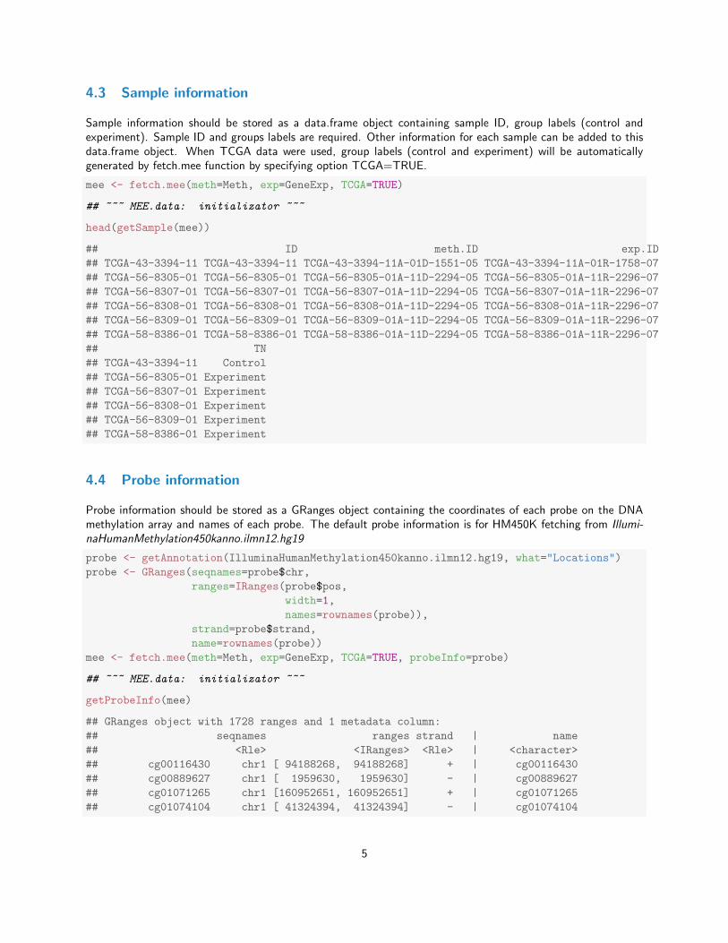
4.3 Sample information
Sample information should be stored as a data.frame object containing sample ID, group labels (control andexperiment). Sample ID and groups labels are required. Other information for each sample can be added to thisdata.frame object. When TCGA data were used, group labels (control and experiment) will be automaticallygenerated by fetch.mee function by specifying option TCGA=TRUE.
mee <- fetch.mee(meth=Meth, exp=GeneExp, TCGA=TRUE)
## ~~~ MEE.data: initializator ~~~
head(getSample(mee))
## ID meth.ID exp.ID
## TCGA-43-3394-11 TCGA-43-3394-11 TCGA-43-3394-11A-01D-1551-05 TCGA-43-3394-11A-01R-1758-07
## TCGA-56-8305-01 TCGA-56-8305-01 TCGA-56-8305-01A-11D-2294-05 TCGA-56-8305-01A-11R-2296-07
## TCGA-56-8307-01 TCGA-56-8307-01 TCGA-56-8307-01A-11D-2294-05 TCGA-56-8307-01A-11R-2296-07
## TCGA-56-8308-01 TCGA-56-8308-01 TCGA-56-8308-01A-11D-2294-05 TCGA-56-8308-01A-11R-2296-07
## TCGA-56-8309-01 TCGA-56-8309-01 TCGA-56-8309-01A-11D-2294-05 TCGA-56-8309-01A-11R-2296-07
## TCGA-58-8386-01 TCGA-58-8386-01 TCGA-58-8386-01A-11D-2294-05 TCGA-58-8386-01A-11R-2296-07
## TN
## TCGA-43-3394-11 Control
## TCGA-56-8305-01 Experiment
## TCGA-56-8307-01 Experiment
## TCGA-56-8308-01 Experiment
## TCGA-56-8309-01 Experiment
## TCGA-58-8386-01 Experiment
4.4 Probe information
Probe information should be stored as a GRanges object containing the coordinates of each probe on the DNAmethylation array and names of each probe. The default probe information is for HM450K fetching from Illumi-naHumanMethylation450kanno.ilmn12.hg19
probe <- getAnnotation(IlluminaHumanMethylation450kanno.ilmn12.hg19, what="Locations")
probe <- GRanges(seqnames=probe$chr,
ranges=IRanges(probe$pos,
width=1,
names=rownames(probe)),
strand=probe$strand,
name=rownames(probe))
mee <- fetch.mee(meth=Meth, exp=GeneExp, TCGA=TRUE, probeInfo=probe)
## ~~~ MEE.data: initializator ~~~
getProbeInfo(mee)
## GRanges object with 1728 ranges and 1 metadata column:
## seqnames ranges strand | name
## <Rle> <IRanges> <Rle> | <character>
## cg00116430 chr1 [ 94188268, 94188268] + | cg00116430
## cg00889627 chr1 [ 1959630, 1959630] - | cg00889627
## cg01071265 chr1 [160952651, 160952651] + | cg01071265
## cg01074104 chr1 [ 41324394, 41324394] - | cg01074104
5

## cg01393939 chr1 [ 87803705, 87803705] + | cg01393939
## ... ... ... ... ... ...
## cg27584013 chr1 [ 23012439, 23012439] + | cg27584013
## cg27589988 chr1 [215147891, 215147891] + | cg27589988
## cg27637706 chr1 [ 3472204, 3472204] - | cg27637706
## ch.1.131529R chr1 [ 3283394, 3283394] + | ch.1.131529R
## ch.1.173213985R chr1 [174947362, 174947362] + | ch.1.173213985R
## -------
## seqinfo: 24 sequences from an unspecified genome; no seqlengths
4.5 Gene information
Gene information should be stored as a GRanges object containing coordinates of each gene, gene id, gene symboland gene isoform id. The default gene information is the UCSC gene annotation fetching from Homo.sapiens byELMER function: txs.
geneAnnot <- txs()
## ’select()’ returned 1:1 mapping between keys and columns
## In TCGA expression data, geneIDs were used as the rowname for each row. However, numbers
## can't be the rownames, "ID" was added to each gene id functioning as the rowname.
## If your geneID is consistent with the rownames of the gene expression matrix, adding "ID"
## to each geneID can be skipped.
geneAnnot$GENEID <- paste0("ID",geneAnnot$GENEID)
geneInfo <- promoters(geneAnnot,upstream = 0, downstream = 0)
save(geneInfo,file="./ELMER.example/Result/LUSC/geneAnnot.rda")
mee <- fetch.mee(meth=Meth, exp=GeneExp, TCGA=TRUE, geneInfo=geneInfo)
## ~~~ MEE.data: initializator ~~~
getGeneInfo(mee)
## GRanges object with 14046 ranges and 3 metadata columns:
## seqnames ranges strand | GENEID TXNAME SYMBOL
## <Rle> <IRanges> <Rle> | <character> <character> <character>
## [1] chr1 [ 69091, 69090] + | ID79501 uc001aal.1 OR4F5
## [2] chr1 [322037, 322036] + | ID100133331 uc009vjk.2 LOC100133331
## [3] chr1 [324288, 324287] + | ID100133331 uc021oeh.1 LOC100133331
## [4] chr1 [367659, 367658] + | ID729759 uc010nxu.2 OR4F29
## [5] chr1 [762971, 762970] + | ID643837 uc031pjj.1 LINC01128
## ... ... ... ... ... ... ... ...
## [14042] chrUn_gl000223 [119731, 119730] - | ID7574 uc031tgh.1 ZNF26
## [14043] chrUn_gl000228 [ 76142, 76141] + | ID22947 uc031tgj.1 DUX4L1
## [14044] chrUn_gl000228 [ 82754, 82753] + | ID22947 uc031tgl.1 DUX4L1
## [14045] chrUn_gl000228 [105896, 105895] + | ID22947 uc031tgq.1 DUX4L1
## [14046] chrUn_gl000228 [109202, 109201] + | ID22947 uc031tgr.1 DUX4L1
## -------
## seqinfo: 93 sequences (1 circular) from hg19 genome
6

4.6 MEE.data
MEE.data object is the input for multiple main functions of ELMER. MEE.data contains the above 5 componentsand making MEE.data object by fetch.mee function will keep each component consistent with each other. Forexample, althougth DNA methylation and gene expression matrixes have different rows (probe for DNA methyla-tion and geneid for gene expression), the column (samples) order should be same in the two matrixes. fetch.meefunction will keep them consistent when it generates the MEE.data object.
mee <- fetch.mee(meth=Meth, exp=GeneExp, TCGA=TRUE, probeInfo=probe, geneInfo=geneInfo)
## ~~~ MEE.data: initializator ~~~
mee
## *** Class MEE.data, method show ***
## * meth
## num [1:1728, 1:234] 0.819 0.842 0.91 0.875 0.333 ...
## - attr(*, "dimnames")=List of 2
## ..$ : chr [1:1728] "cg00045114" "cg00050294" "cg00066722" "cg00093522" ...
## ..$ : chr [1:234] "TCGA-43-3394-11A-01D-1551-05" "TCGA-56-8305-01A-11D-2294-05" "TCGA-56-8307-01A-11D-2294-05" "TCGA-56-8308-01A-11D-2294-05" ...
## NULL
## * exp
## num [1:3884, 1:234] 0 0.214 10.048 5.007 8.63 ...
## - attr(*, "dimnames")=List of 2
## ..$ : chr [1:3884] "ID126767" "ID343066" "ID26574" "ID24" ...
## ..$ : chr [1:234] "TCGA-43-3394-11A-01R-1758-07" "TCGA-56-8305-01A-11R-2296-07" "TCGA-56-8307-01A-11R-2296-07" "TCGA-56-8308-01A-11R-2296-07" ...
## NULL
## * sample
## 'data.frame': 234 obs. of 4 variables:
## $ ID : chr "TCGA-43-3394-11" "TCGA-56-8305-01" "TCGA-56-8307-01" "TCGA-56-8308-01" ...
## $ meth.ID: chr "TCGA-43-3394-11A-01D-1551-05" "TCGA-56-8305-01A-11D-2294-05" "TCGA-56-8307-01A-11D-2294-05" "TCGA-56-8308-01A-11D-2294-05" ...
## $ exp.ID : chr "TCGA-43-3394-11A-01R-1758-07" "TCGA-56-8305-01A-11R-2296-07" "TCGA-56-8307-01A-11R-2296-07" "TCGA-56-8308-01A-11R-2296-07" ...
## $ TN : chr "Control" "Experiment" "Experiment" "Experiment" ...
## NULL
## * probeInfo
## GRanges object with 1728 ranges and 1 metadata column:
## seqnames ranges strand | name
## <Rle> <IRanges> <Rle> | <character>
## cg00116430 chr1 [ 94188268, 94188268] + | cg00116430
## cg00889627 chr1 [ 1959630, 1959630] - | cg00889627
## cg01071265 chr1 [160952651, 160952651] + | cg01071265
## cg01074104 chr1 [ 41324394, 41324394] - | cg01074104
## cg01393939 chr1 [ 87803705, 87803705] + | cg01393939
## ... ... ... ... ... ...
## cg27584013 chr1 [ 23012439, 23012439] + | cg27584013
## cg27589988 chr1 [215147891, 215147891] + | cg27589988
## cg27637706 chr1 [ 3472204, 3472204] - | cg27637706
## ch.1.131529R chr1 [ 3283394, 3283394] + | ch.1.131529R
## ch.1.173213985R chr1 [174947362, 174947362] + | ch.1.173213985R
## -------
## seqinfo: 24 sequences from an unspecified genome; no seqlengths
## * geneInfo
## GRanges object with 14046 ranges and 3 metadata columns:
7

## seqnames ranges strand | GENEID TXNAME SYMBOL
## <Rle> <IRanges> <Rle> | <character> <character> <character>
## [1] chr1 [ 69091, 69090] + | ID79501 uc001aal.1 OR4F5
## [2] chr1 [322037, 322036] + | ID100133331 uc009vjk.2 LOC100133331
## [3] chr1 [324288, 324287] + | ID100133331 uc021oeh.1 LOC100133331
## [4] chr1 [367659, 367658] + | ID729759 uc010nxu.2 OR4F29
## [5] chr1 [762971, 762970] + | ID643837 uc031pjj.1 LINC01128
## ... ... ... ... ... ... ... ...
## [14042] chrUn_gl000223 [119731, 119730] - | ID7574 uc031tgh.1 ZNF26
## [14043] chrUn_gl000228 [ 76142, 76141] + | ID22947 uc031tgj.1 DUX4L1
## [14044] chrUn_gl000228 [ 82754, 82753] + | ID22947 uc031tgl.1 DUX4L1
## [14045] chrUn_gl000228 [105896, 105895] + | ID22947 uc031tgq.1 DUX4L1
## [14046] chrUn_gl000228 [109202, 109201] + | ID22947 uc031tgr.1 DUX4L1
## -------
## seqinfo: 93 sequences (1 circular) from hg19 genome
## ******* End Print (MEE.data) *******
5 Illustration of ELMER analysis steps
The example data set is a subset of chromosome 1 data from TCGA LUSC. ELMER analysis have 5 main stepswhich are shown below individually. TCGA.pipe introduced above is a pipeline combining all 5 steps and producingall results and figures.
5.1 Selection of probes within biofeatures
This step is to select HM450K probes, which locate far from TSS (at least 2Kb away) and within distal enhancerregions. These probes are called distal enhancer probes. For distal enhancer regions, we constructed a compre-hensive list of putative enhancers combining REMC, ENCODE and FANTOM5 data. Enhancers were identifiedusing ChromHMM for 98 tissues or cell lines from REMC and ENCODE project and we used the union of genomicelements labeled as EnhG1, EnhG2, EnhA1 or EnhA2 (representing intergenic and intragenic active enhancers)in any of the 98 cell types, resulting in a total of 389,967 non-overlapping enhancer regions. Additionally, FAN-TOM5 enhancers (43,011) identified by eRNAs for 400 distinct cell types were added to this list. Be default, thiscomprehensive list of putative enhancer and TSS annotated by GENCODE V15 and UCSC-gene will be used toselect distal enhancer probes. But user can use their own TSS annotation or features such as H3K27ac ChIP-seqin a certain cell line.
#get distal enhancer probes that are 2kb away from TSS and overlap with REMC and FANTOM5
#enhancers on chromosome 1
Probe <- get.feature.probe(rm.chr=paste0("chr",c(2:22,"X","Y")))
save(Probe,file="./ELMER.example/Result/LUSC/probeInfo_feature_distal.rda")
5.2 Identifying differentially methylated probes
This step is to identify DNA methylation changes at distal enhancer probes which is carried out by functionget.diff.meth.
For each enhancer probe, function first ranked experiment samples and control samples by their DNA methylationbeta values. To identify hypomethylated probes, function compared the lower control quintile (20% of control
8
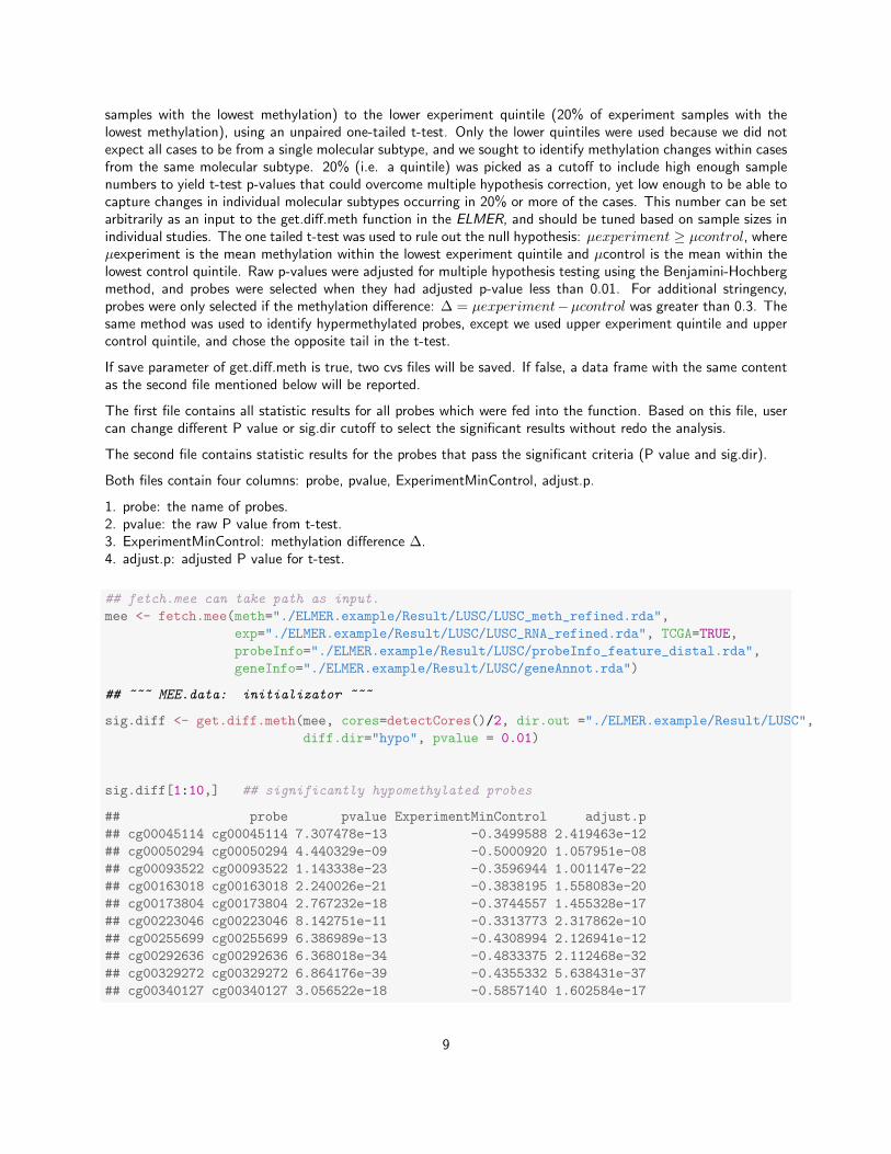
samples with the lowest methylation) to the lower experiment quintile (20% of experiment samples with thelowest methylation), using an unpaired one-tailed t-test. Only the lower quintiles were used because we did notexpect all cases to be from a single molecular subtype, and we sought to identify methylation changes within casesfrom the same molecular subtype. 20% (i.e. a quintile) was picked as a cutoff to include high enough samplenumbers to yield t-test p-values that could overcome multiple hypothesis correction, yet low enough to be able tocapture changes in individual molecular subtypes occurring in 20% or more of the cases. This number can be setarbitrarily as an input to the get.diff.meth function in the ELMER, and should be tuned based on sample sizes inindividual studies. The one tailed t-test was used to rule out the null hypothesis: µexperiment ≥ µcontrol, whereµexperiment is the mean methylation within the lowest experiment quintile and µcontrol is the mean within thelowest control quintile. Raw p-values were adjusted for multiple hypothesis testing using the Benjamini-Hochbergmethod, and probes were selected when they had adjusted p-value less than 0.01. For additional stringency,probes were only selected if the methylation difference: ∆ = µexperiment−µcontrol was greater than 0.3. Thesame method was used to identify hypermethylated probes, except we used upper experiment quintile and uppercontrol quintile, and chose the opposite tail in the t-test.
If save parameter of get.diff.meth is true, two cvs files will be saved. If false, a data frame with the same contentas the second file mentioned below will be reported.
The first file contains all statistic results for all probes which were fed into the function. Based on this file, usercan change different P value or sig.dir cutoff to select the significant results without redo the analysis.
The second file contains statistic results for the probes that pass the significant criteria (P value and sig.dir).
Both files contain four columns: probe, pvalue, ExperimentMinControl, adjust.p.
1. probe: the name of probes.2. pvalue: the raw P value from t-test.3. ExperimentMinControl: methylation difference ∆.4. adjust.p: adjusted P value for t-test.
## fetch.mee can take path as input.
mee <- fetch.mee(meth="./ELMER.example/Result/LUSC/LUSC_meth_refined.rda",
exp="./ELMER.example/Result/LUSC/LUSC_RNA_refined.rda", TCGA=TRUE,
probeInfo="./ELMER.example/Result/LUSC/probeInfo_feature_distal.rda",
geneInfo="./ELMER.example/Result/LUSC/geneAnnot.rda")
## ~~~ MEE.data: initializator ~~~
sig.diff <- get.diff.meth(mee, cores=detectCores()/2, dir.out ="./ELMER.example/Result/LUSC",
diff.dir="hypo", pvalue = 0.01)
sig.diff[1:10,] ## significantly hypomethylated probes
## probe pvalue ExperimentMinControl adjust.p
## cg00045114 cg00045114 7.307478e-13 -0.3499588 2.419463e-12
## cg00050294 cg00050294 4.440329e-09 -0.5000920 1.057951e-08
## cg00093522 cg00093522 1.143338e-23 -0.3596944 1.001147e-22
## cg00163018 cg00163018 2.240026e-21 -0.3838195 1.558083e-20
## cg00173804 cg00173804 2.767232e-18 -0.3744557 1.455328e-17
## cg00223046 cg00223046 8.142751e-11 -0.3313773 2.317862e-10
## cg00255699 cg00255699 6.386989e-13 -0.4308994 2.126941e-12
## cg00292636 cg00292636 6.368018e-34 -0.4833375 2.112468e-32
## cg00329272 cg00329272 6.864176e-39 -0.4355332 5.638431e-37
## cg00340127 cg00340127 3.056522e-18 -0.5857140 1.602584e-17
9
# get.diff.meth automatically save output files.
# getMethdiff.hypo.probes.csv contains statistics for all the probes.
# getMethdiff.hypo.probes.significant.csv contains only the significant probes which
# is the same with sig.diff
dir(path = "./ELMER.example/Result/LUSC", pattern = "getMethdiff")
## [1] "getMethdiff.hypo.probes.csv" "getMethdiff.hypo.probes.significant.csv"
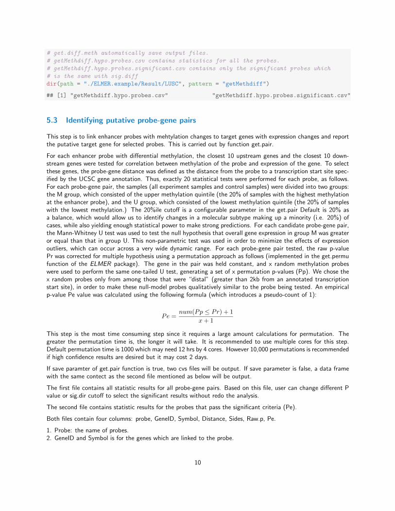
5.3 Identifying putative probe-gene pairs
This step is to link enhancer probes with mehtylation changes to target genes with expression changes and reportthe putative target gene for selected probes. This is carried out by function get.pair.
For each enhancer probe with differential methylation, the closest 10 upstream genes and the closest 10 down-stream genes were tested for correlation between methylation of the probe and expression of the gene. To selectthese genes, the probe-gene distance was defined as the distance from the probe to a transcription start site spec-ified by the UCSC gene annotation. Thus, exactly 20 statistical tests were performed for each probe, as follows.For each probe-gene pair, the samples (all experiment samples and control samples) were divided into two groups:the M group, which consisted of the upper methylation quintile (the 20% of samples with the highest methylationat the enhancer probe), and the U group, which consisted of the lowest methylation quintile (the 20% of sampleswith the lowest methylation.) The 20%ile cutoff is a configurable parameter in the get.pair Default is 20% asa balance, which would allow us to identify changes in a molecular subtype making up a minority (i.e. 20%) ofcases, while also yielding enough statistical power to make strong predictions. For each candidate probe-gene pair,the Mann-Whitney U test was used to test the null hypothesis that overall gene expression in group M was greateror equal than that in group U. This non-parametric test was used in order to minimize the effects of expressionoutliers, which can occur across a very wide dynamic range. For each probe-gene pair tested, the raw p-valuePr was corrected for multiple hypothesis using a permutation approach as follows (implemented in the get.permufunction of the ELMER package). The gene in the pair was held constant, and x random methylation probeswere used to perform the same one-tailed U test, generating a set of x permutation p-values (Pp). We chose thex random probes only from among those that were “distal” (greater than 2kb from an annotated transcriptionstart site), in order to make these null-model probes qualitatively similar to the probe being tested. An empiricalp-value Pe value was calculated using the following formula (which introduces a pseudo-count of 1):
Pe =num(Pp ≤ Pr) + 1
x+ 1
This step is the most time consuming step since it requires a large amount calculations for permutation. Thegreater the permutation time is, the longer it will take. It is recommended to use multiple cores for this step.Default permutation time is 1000 which may need 12 hrs by 4 cores. However 10,000 permutations is recommendedif high confidence results are desired but it may cost 2 days.
If save paramter of get.pair function is true, two cvs files will be output. If save parameter is false, a data framewith the same contect as the second file mentioned as below will be output.
The first file contains all statistic results for all probe-gene pairs. Based on this file, user can change different Pvalue or sig.dir cutoff to select the significant results without redo the analysis.
The second file contains statistic results for the probes that pass the significant criteria (Pe).
Both files contain four columns: probe, GeneID, Symbol, Distance, Sides, Raw.p, Pe.
1. Probe: the name of probes.2. GeneID and Symbol is for the genes which are linked to the probe.
10

3. Distance: the distance between the probe and the gene.4. Sides: right (R) side or left (L) side of probe and the rank based on distance. For example, L3 means the geneis the number 3 closest gene from the left side of the probe.5. Raw.p: P value from the Mann-Whitney U test for each pair.6. Pe: the empirical P value for each pair.
### identify target gene for significantly hypomethylated probes.
Sig.probes <- read.csv("./ELMER.example/Result/LUSC/getMethdiff.hypo.probes.significant.csv",
stringsAsFactors=FALSE)[,1]
head(Sig.probes) # significantly hypomethylated probes
## [1] "cg00045114" "cg00050294" "cg00093522" "cg00163018" "cg00173804" "cg00223046"
## Collect nearby 20 genes for Sig.probes
nearGenes <-GetNearGenes(TRange=getProbeInfo(mee,probe=Sig.probes),
geneAnnot=getGeneInfo(mee),cores=detectCores()/2)
## Identify significant probe-gene pairs
Hypo.pair <-get.pair(mee=mee,probes=Sig.probes,nearGenes=nearGenes,
permu.dir="./ELMER.example/Result/LUSC/permu",permu.size=300,Pe = 0.01,
dir.out="./ELMER.example/Result/LUSC",cores=detectCores()/2,label= "hypo")
## Calculate empirical P value.
head(Hypo.pair) ## significant probe-gene pairs
## Probe GeneID Symbol Distance Sides Raw.p Pe
## cg20701183.ID8543 cg20701183 ID8543 LMO4 2563 L2 7.453984e-14 0.003322259
## cg19403323.ID255928 cg19403323 ID255928 SYT14 87458 R1 1.671937e-12 0.003322259
## cg12213388.ID84451 cg12213388 ID84451 KIAA1804 993548 L4 2.527644e-12 0.003322259
## cg26607897.ID55811 cg26607897 ID55811 ADCY10 292476 R4 4.593610e-12 0.003322259
## cg10574861.ID8543 cg10574861 ID8543 LMO4 4715 L2 4.770162e-12 0.003322259
## cg26607897.ID23432 cg26607897 ID23432 GPR161 563308 R7 8.048248e-12 0.003322259
# get.pair automatically save output files.
#getPair.hypo.all.pairs.statistic.csv contains statistics for all the probe-gene pairs.
#getPair.hypo.pairs.significant.csv contains only the significant probes which is
# same with Hypo.pair.
dir(path = "./ELMER.example/Result/LUSC", pattern = "getPair")
## [1] "getPair.hypo.all.pairs.statistic.csv"
## [2] "getPair.hypo.pairs.significant.csv"
## [3] "getPair.hypo.pairs.significant.withmotif.csv"
5.4 Motif enrichment analysis on the selected probes
This step is to identify enriched motif in a set of probes which is carried out by function get.enriched.motif.
The build in data Probes.motif is generated using FIMO with a p-value ¡ 1e–4 to scan a +/- 100bp region aroundeach probe using Factorbook motif position weight matrices (PWMs) and Jasper core human motif PWMsgenerated from the R package MotifDb. For each probe set tested (i.e. the list of gene-linked hypomethylatedprobes in a given experiment group), a motif enrichment Odds Ratio and a 95% confidence interval were calculated
11
using following formulas:
p =a
a+ b
P =c
c+ d
Odds Ratio =
p1−p
P1−P
SD =
√1
a+
1
b+
1
c+
1
d
lower boundary of 95% confidence interval = exp (lnOR− SD)
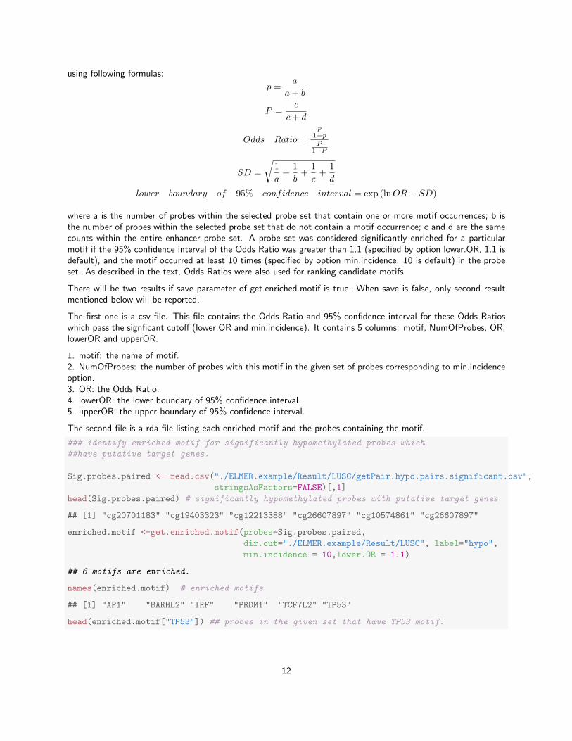
where a is the number of probes within the selected probe set that contain one or more motif occurrences; b isthe number of probes within the selected probe set that do not contain a motif occurrence; c and d are the samecounts within the entire enhancer probe set. A probe set was considered significantly enriched for a particularmotif if the 95% confidence interval of the Odds Ratio was greater than 1.1 (specified by option lower.OR, 1.1 isdefault), and the motif occurred at least 10 times (specified by option min.incidence. 10 is default) in the probeset. As described in the text, Odds Ratios were also used for ranking candidate motifs.
There will be two results if save parameter of get.enriched.motif is true. When save is false, only second resultmentioned below will be reported.
The first one is a csv file. This file contains the Odds Ratio and 95% confidence interval for these Odds Ratioswhich pass the signficant cutoff (lower.OR and min.incidence). It contains 5 columns: motif, NumOfProbes, OR,lowerOR and upperOR.
1. motif: the name of motif.2. NumOfProbes: the number of probes with this motif in the given set of probes corresponding to min.incidenceoption.3. OR: the Odds Ratio.4. lowerOR: the lower boundary of 95% confidence interval.5. upperOR: the upper boundary of 95% confidence interval.
The second file is a rda file listing each enriched motif and the probes containing the motif.
### identify enriched motif for significantly hypomethylated probes which
##have putative target genes.
Sig.probes.paired <- read.csv("./ELMER.example/Result/LUSC/getPair.hypo.pairs.significant.csv",
stringsAsFactors=FALSE)[,1]
head(Sig.probes.paired) # significantly hypomethylated probes with putative target genes
## [1] "cg20701183" "cg19403323" "cg12213388" "cg26607897" "cg10574861" "cg26607897"
enriched.motif <-get.enriched.motif(probes=Sig.probes.paired,
dir.out="./ELMER.example/Result/LUSC", label="hypo",
min.incidence = 10,lower.OR = 1.1)
## 6 motifs are enriched.
names(enriched.motif) # enriched motifs
## [1] "AP1" "BARHL2" "IRF" "PRDM1" "TCF7L2" "TP53"
head(enriched.motif["TP53"]) ## probes in the given set that have TP53 motif.
12
## $TP53
## [1] "cg18437839" "cg11718886" "cg18437839" "cg22684969" "cg11718886" "cg06358191"
## [7] "cg11718886" "cg18161025" "cg11718886" "cg04923840" "cg24729839" "cg24296187"
## [13] "cg23972860" "cg18437839" "cg09858925" "cg06358191" "cg11718886" "cg06358191"
## [19] "cg11718886" "cg09858925" "cg18161025" "cg17181043" "cg22684969" "cg09858925"
## [25] "cg07347148" "cg06358191" "cg09874992" "cg11718886" "cg11958234" "cg17181043"
## [31] "cg00974095" "cg14420230" "cg11718886" "cg22684969" "cg18795022" "cg24296187"
## [37] "cg25001190" "cg07381872" "cg24296187" "cg02837162" "cg25001190" "cg24296187"
## [43] "cg20284239" "cg00935967" "cg11157208" "cg09814448" "cg11157208" "cg04105712"
## [49] "cg04105712"
# get.enriched.motif automatically save output files.
# getMotif.hypo.enriched.motifs.rda contains enriched motifs and the probes with the motif.
# getMotif.hypo.motif.enrichment.csv contains summary of enriched motifs.
dir(path = "./ELMER.example/Result/LUSC", pattern = "getMotif")
## [1] "getMotif.hypo.enriched.motifs.rda" "getMotif.hypo.motif.enrichment.csv"
# motif enrichment figure will be automatically generated.
dir(path = "./ELMER.example/Result/LUSC", pattern = "motif.enrichment.pdf")
## [1] "hypo.motif.enrichment.pdf"
5.5 Identifying regulatory TFs
This step is to identify regulatory TF whose expression associates with TF binding motif DNA methylation whichis carried out by function get.TFs.For each motif considered to be enriched within a particular probe set, function will compare the average DNAmethylation at all distal enhancer probes within +/- 100bp of a motif occurrence, to the expression of 1,982human TFs A statistical test was performed for each motif-TF pair, as follows. The samples (all control andexperiment samples) were divided into two groups: the M group, which consisted of the 20% of samples withthe highest average methylation at all motif-adjacent probes, and the U group, which consisted of the 20% ofsamples with the lowest methylation. The 20th percentile cutoff is a parameter to the get.TFs function and wasset to allow for identification of molecular subtypes present in 20% of cases. For each candidate motif-TF pair,the Mann-Whitney U test was used to test the null hypothesis that overall gene expression in group M was greateror equal than that in group U. This non-parametric test was used in order to minimize the effects of expressionoutliers, which can occur across a very wide dynamic range. For each motif tested, this resulted in a raw p-value(Pr) for each of the 1982 TFs. All TFs were ranked by the -log10(Pr), and those falling within the top 5% ofthis ranking were considered candidate upstream regulators. The best upstream TFs which are known recognizedthe motif was automatically extracted as putative regulatory TFs.
If save parameter of get.TFs function is true, two files will be generated. If save parameter is false, only a dataframe containing the same content with the first file mentioned below will be output.
The first one csv file. This file contain the regulatory TF significantly associate with average DNA methylationat particular motif sites. It contains 4 columns: motif, top.potential.TF, potential.TFs and top 5percent.
1. motif: the names of motif.2. top.potential.TF: the highest ranking upstream TFs which are known recognized the motif.3. potential.TFs: TFs which are within top 5% list and are known recognized the motif.4. top 5percent: all TFs which are within top 5% list.
The second file is rda file. This file contains a matrix storing the statistic results for associations between TFs
13
(row) and average DNA methylation at motifs (column). This matrix can be use to generate TF ranking plotsby function TF.rank.plot.
### identify regulatory TF for the enriched motifs
load("./ELMER.example/Result/LUSC/getMotif.hypo.enriched.motifs.rda")
TF <- get.TFs(mee=mee, enriched.motif=enriched.motif,dir.out="./ELMER.example/Result/LUSC",
cores=detectCores()/2, label= "hypo")
# get.TFs automatically save output files.
# getTF.hypo.TFs.with.motif.pvalue.rda contains statistics for all TF with average
# DNA methylation at sites with the enriched motif.
# getTF.hypo.significant.TFs.with.motif.summary.csv contains only the significant probes.
dir(path = "./ELMER.example/Result/LUSC", pattern = "getTF")
## [1] "getTF.hypo.TFs.with.motif.pvalue.rda"
## [2] "getTF.hypo.significant.TFs.with.motif.summary.csv"
# TF ranking plot based on statistics will be automatically generated.
dir(path = "./ELMER.example/Result/LUSC/TFrankPlot", pattern = "pdf")
## [1] "BCL11A.TFrankPlot.pdf" "DMRT2.TFrankPlot.pdf" "FOXN1.TFrankPlot.pdf"
## [4] "MCM5.TFrankPlot.pdf" "NFE2L2.TFrankPlot.pdf" "OTX1.TFrankPlot.pdf"
## [7] "PIR.TFrankPlot.pdf" "PRICKLE3.TFrankPlot.pdf" "SMARCB1.TFrankPlot.pdf"
## [10] "SOX21.TFrankPlot.pdf" "TADA2A.TFrankPlot.pdf" "TP63.TFrankPlot.pdf"
## [13] "TTF2.TFrankPlot.pdf" "ZFP64.TFrankPlot.pdf"
14
6 Generating figures
6.1 Scatter plots
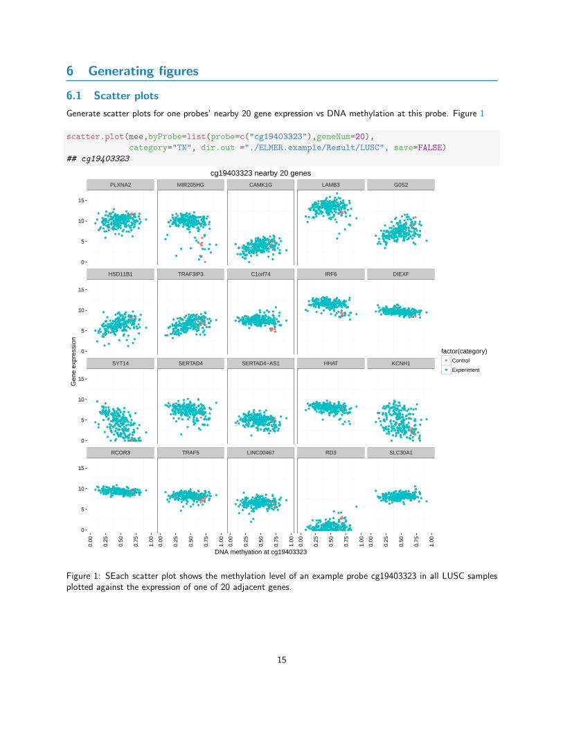
Generate scatter plots for one probes’ nearby 20 gene expression vs DNA methylation at this probe. Figure 1
scatter.plot(mee,byProbe=list(probe=c("cg19403323"),geneNum=20),
category="TN", dir.out ="./ELMER.example/Result/LUSC", save=FALSE)
## cg19403323
●
●
●
●
●●
●
●
●●
●
●
●
●
●●
●●●
● ●●
●
●
●●
●
●
●
●●
● ●
●
●
●
●
●
●
●
●●
●
●
●●
●●
●
●
●
●
●
●
●
●
●
●
●●
●
●
●●●
●
●
●
●●●
●
●
●
●
●
●
●
●
●
●
●
●
●●
●
●
●
●●
●
●●
●
●
●
●
●
●
●
●
●
●
●
●
●
●
●
●
●
●
●
●●
●
●
●●
●
●●
●●
●
●●●
●●●●
●
●
●
●
●
●●
●●
●
●
●
●●●
●●
●●
●● ●
●
●
●
●
●
●
●●
●●
●
●●
●
●
●●●
●
●
●
●
●●
●
●
●●
●●
●
●
●
●
●
●●
●●
●
●
●●
●
●●●●
●
● ●●
●●
● ●
●
●●
●●
●
●
●
●
●
●
●
●
●
●
●●
●
● ●●
●●
●
●
●
●● ●
●●
●
●●
●
●
●●
●
●● ●
●
●●
●●
●
●
●
●
●
●
●●
●
●
●●
●
●
●
●
● ●●
●
●●
●● ●
●
●
●
●
● ●●
●
●
●
●
●
●● ● ●
●
●
●
●
●
●
●
●
●
●
●
●
●
●●
●
●
●
●
●
●
●●
●
●
●
●●
●
●
●
●●●
●
●●
●●
●
●●●
●
●
●
●
●
●
●
●
●
●
●
●
●
●
●
●
●
●
●
●●
●●
●
●
●
●●
●
●
●●
●●
●
●●
●
●
●
●
●
●
●
●●
●●
●●
●
●
●
●
●
●
●
●●
●
●
●
●
●
●
●
●
●
●
●
●
●
●
●
●
●●
●
● ●●●
●●
●
●
●
●
●
●
●
●
●
●
●
●
●
●●
●
●● ●●
●●
●●
●●
●●
●
●
●●
●
●
●
●
●●
●● ●
● ●●
●●
●
●●
●●●
●
●
●●
●●
●
●
●
●●
●
●
●●
●
●
● ●
●
●
●● ●
●
●
●
●
●●
●
●●
● ●●
●
●
●
●●
●
●●
●
●
●
●
●
●
●
●●
● ●
●
●
●
●
●
●
●
●
●
●
●
●
●
●
●
●
●
●
●
●
●●
●
●
●
●
●● ● ●● ●
●
●
●
●
● ●
●
●
●
●
●
●
●
●
●
●
●●
●
●
●
●
●●●
●
●●
●
●
●
●
●
●
●
●
●
●
●
●
●
●
●
●●
●
●●
●
●●●
●●
●
●●
●
●
●
● ●
●
●●
●
●●
●
●●
●
● ●
●●●
●
●
●
●
●
●
●
●
●
●●
●●
●●
●
●
●
●
●●
●
●
●
●
●
●●
●
●
●
●
●
●●
●
●● ●
●
●●
●●
●
●●
●●
●●
● ●
●
●
●●
●
●
●
●
●
●
●●
● ●
●●
●
●
●
●
●
●●
●●
●
●
●
●
●●
●●
●●
●●●
●
●
●
●
● ●
●
●
●
●
●
●
●
●● ●
● ●
●
●
●
●
●
●
●●
●●●
●
●●
●
●
●●
●
●
●
●●
●
●●
●●
●
●
●
●
●●
●
●●●
●●
●
●●
●
●
●
●
●● ●
●
●
●
●
●
●
●
●
●
●●
●
●
●
●
●
●●
●
●●
●
●
●
●
●
●
●
●
●
●
●
●
●●
●
●
● ●
●
●
●
●
●
●
●●
●
●
●
●
●
● ●
●
●
●
●●
●
●
●●
●
●●
●
●
●
●
●
●
●●
●
●●
●●
●
●
●
●
●●●
●
●
●
●
●
●●
●
● ●
●
●
●●
●
●
●
● ●
●
●
●
●
●
●
●●
●
●
●
●
●
●
●
●
●
●
●
●
●
●
●●
● ●●
●
●
●
●
●
●
●
●
●
●●●
●
●●
●
●●
●
●
●
●
●
●
●
●
●
●
●
●
●●
●
●
●
● ●
●
●
●●
●
●
● ●
●
●
●
● ●●
●
●
●
●
●
●
●
●
●
●
●●
●
●●
● ●
●
●
●
●●
●
●
●
●
●
●
●
●
●●
●
●
●●
●
●
●
●
●
●
●
●● ●
●
●
●●
●●
●
●
●●
●
●●
●
●
●
●
●●
●
●
●
●
●
●
● ●●●
●
●
●
●●●●
●
●
●
●●
●●
●
●●
●
●
●
●
●
●
●●
●
●
●
●●
●
●●
●
●
●
●
●●
●●
●
●
●
●
●
●
●
●
●
● ● ●
●
●
●
●
●
●
●
●
●
●
●
●
●
● ●●
●
●
●
●
●
●
●●●
●
●
●●
●
●
●
●
●
●
●
●
●●●●
●●
●●
●●
●
●
● ●●
●
●●
●
●
●
●
●
●
●● ● ●●
●
●
●●
●
●●
●●●
● ●
●
●●●
●
●
●
●
●
●
●
●
●
●
●
●
●
●
●
●
●
●●
●●
●
●●
●
●
●
●
●
●
●
●● ●
●
●
●
●
●●
●
●●●
●●
●
●
●
●
●
● ●
●
●
●
●
●
●●
●
●
●
●
●
●
●
●●
●
●
●
●● ●
●
●
●
●
●
●
●●
●
●
●
●
●●
●
●
●●
●
●
●
●
●
● ●●●
●
●
●
●
●
●
●
●
●
●
●
●
●
●
●
●
●
●●
●
●
●
●●
●
●
●
●
●●
●
●
●
●
●●
●
●●
● ●
●
●
●
●
●
●●
●●
●
●
●
●
●
●
●●
●
●
●
●●
●
●●
●
●
●
●
●
●
●●
●
●
● ●●
●
●
●
●
●
●●
●
●
●
●●
●●●
●
●
●●
●
●
●
●
● ●
●●
●
●●
●●
●
●●
●
●
●
●●●
●
●
●
●●
●
●
●
●●
●
●●●
●
●
●●
●
●●
●
●
●
●
●
●●
●
●●
●
●
●
●●
●
●●
● ●●
●
●
●
●
●
●
●
●
●
●
●
●
●
●
●●
●●
●
●
●
●
●
●
●
●
●
●
●
●
●
●●
●
●
●
●
●
●
● ●●
●
●
●
●
●●
●
●
●
●
●
●
● ●●
●●
●●● ●
●
●
●●
●
●●
●●
●
●●
●
●
●
●
●
●
●
●
●
●
●
●
●●
●
●●●
●
●
●
●
● ●
●
●
●
●
●●
●
●●
●
●
●
●●
●
●
●
●●
●
●
●
●
●
●
●
●
●
●
●●
●
●
●●●
●●
●
●
●
●●
●
●
●●
●
●
●
●
●
●
●
●
●●
●
● ●● ●●
●●●
●
●
●
●●
●
●
●
●
●
●●
●
●●●
●
●
●●
● ●
●●
●
●
●
●●
●●
●
●●
●
●●
●●
●
●●
●
●●
●
●●
●
●
●●
●
●
●
●
●●● ●●
●
●
●
●
●
●
●
●
●●
● ●
●●●
●
● ●
●
●●
●
●
●
●
●
●
●
●●●
●
●●
●
●●
●
●
●
●●
●●
●
●●●
●
●●
● ●●
●
●
● ●
●
●
● ●
●
●
●
●●
●
●●
●
●
●● ●●
●●
●
● ●●
●
●● ●●
●
● ●●
●
●
● ●●
●
●
●
●
●
●
●●
●●
●●
●●●●
●
●●
●
●
●●
●
●
●
●●
●●
●● ●
●
●●
●
●
●●
●●
●●
●
●
●● ●
●
●
●
●
●
●
●
●
●●
●
●
●
●●
●
●
●●
●
● ●
●
●
●
●
●●
●
●
●
●●●
●●
● ●● ●
●●
● ●
●
●
●● ●
●
●
●●
●●●
● ●●
●
● ●
●
●
●
●
●
●
● ●●
●●
●
●●
●●●
● ●
●●●
●
●
●
●●
●●
●
●
●
●
●
● ●●
●
●
●●
●
●
●
●
● ●
●●
●
●
●
●
●
●
●●
●
●
●
●
●
●
●
●
●
●
●●
●
●
●
●●
● ●
●●●
●
●
●●
●
●
●
●
● ●●
●
●
●●
●
●
●
●
●
●●
●
●●
●
●
●●●
●
●
●
●●
●
● ●
● ●
●
●●●
●
●
●● ●
●
●●
●
●
●
●
●●
●●
●●●●
●●
●
●●
●
●
●
●
●
●
●
●
●
● ●
●
●
● ●
●
●● ●
●
●●● ●●
●
●
●
●
●
●●
●
●
●●
●
●
●
●
●
●
●
●
●
●
●
●●
●●
●●
●
●
●●●●
●●● ●
●
●
●●
●●
●
●●
●
●
●● ●●
●
●●
●●●
●●
●●
● ●●
● ●
●
●●●
●●
●
●
●●
●
● ●
●
●●●
●
●●
●
●●
●
●
● ●● ●
●●
●●● ●
●
●
●
● ●●
●●●
●
●
●●
●●
●●
●●
●
● ●
●
●
●● ●●
●
●●● ●
●
●●
● ●
● ●
●
●
●●●
●
●
●
●●
●● ●
●
●●
●●
●●●● ●
●
●●●●
●
●
●
● ● ●● ● ●
●
● ●
●
●
●
●●
●●●
●●
●
●
●
●
●
●
●
●● ●●
●●
●
●
●●●● ●●
●●
●●● ●● ●
● ●
●
●● ●●
●●
● ●
●
●
●
●●●●●●
●
●● ●● ●●
●
●● ●
● ●●●
●●
●●
●
●
●
●●●●
●
●● ● ●●
●●
●●
●
●
● ● ●
●
●
●
●
●●
●
●●
●
●
●●
●
●
●
●
●
●
●●
●
●●
●
●
●
●
●●
●
●●●
●●
●
●
●
●
●
●
●
●
●
●
●
●
●
●●
●●
●
●
●
●
●
●
●
●
●
●
●● ●
●●
●
●
●●
●
●●
●
●
●
●
●
●
●
●
●
●
●
●
●
●
●
●
●
●
●
●
●
●
●
●
●
●
●
●●
●
●
●
●
●
●
●
●
●
●
●
●
●
●
●
●
●
●
●
●
●
●
●●
●
●
●
●
●
●
●
●
●●
●●●
●
●
●
●
●
●
●●
●●
●
●
●●
●
●
● ●●
●
●
●
●
●
●
● ●
●
●
●
●
●
●
●
●
●
● ●
●
●
●
●
●
●
●
●
●
●
●
●
●
●
●●
●
●
●●
●
●
●
● ●
●
●
●
●
●
●
●
●●
●●
●
●
●
●
●
●
●
●
●
●●
●
●
●●
●
●
●
●
●●
●
●
●
●
●
●
●
●
●
●
●
●
● ●
●
● ●
●●
●
●
●
●●
● ●● ● ●
●
●
●
●
●
●
●
●
●
● ●
●
●
●
●
●●
●
●
●
●●●● ●
●●
●●
●
●
●●
●
●●
●●
●
●
●
●
●
●
●●
●
●
●
●
●
●
●●●
●
●●
●
●
●●
●
●
●●
●●
●
●
●
●
●
●
●
●
●
●
●
●●
●
●●●
●
●
●
●
●
●
●
●
●
●
●
●●
●
●
●
●
●
●●
●●● ●
● ●
●
●
●●
● ●
●
●●
●
●●
●
●
●●
●
●
●
●●
●
●
●
●
●
●●
●
●●
●
●
●
●
●●
● ●●
●
●
●
●●
●
●
●
●
●
●
●
●
●
●
●
●
●
●
●
●
●
●
●
●
●
●
●●
●
●●
●●
●
●
●●
●
●●
●
●
●
●
●
●●
●
●
●
●●
● ●
●
●
●●
●●
●
● ●
●
●
● ●
●
●
●
●●
●
●
●
●
●
●
●●
●
●
●
●
● ●●●
●
●
●
● ●
●
●●
●
●
●
●
●
●
●
●
●●
●
●
●
●
●
●
●
●●
●
●
●●●
●
●
●
●
●●
●
●
● ●●
●
●
●
●
●
●
●
●●
●
●
●
●
●
●
● ●
●●
● ●
●
●
●●
●
●
●
●
●
●
●
●
●
●
●
●●
●
●●
●●
●
●
●
●
●
● ● ●●●
●
●●
●
●
●
●●●
●
●●
●●
●●
●
●●
●
●
●
●
●
●
●
●
●
●
●
●
●●
●
●
●●
●
●
●●
●
●
●
●●
●●
●●
●
●
●
●
●
●
●
●
●●●
●
●●
●
●
●
●
●
●
●
●
●
●
●
●
●
●●
●
● ●●●
●
●
●
●
●
●
●
●●
●
●
●
●●
●
● ●
●●
●
●
●●● ●
●
●●
●
●●
●●
●●
●
●●
●
●● ●
●
●
●●
●
● ●●● ●
●
●●
●
●
●●
●
●● ●●
●●
●●
●●
●
● ●●
● ●
●●
●
● ●
●
●●
●● ●
●●● ●● ●
●● ●
● ●
●
●
●
●●
●
●
●
●●
●●
●
● ●
● ●
●
● ●
●
●●
●
●●
●
●
●
●
●● ●●
●
●
●
●
●●●●
●
●
●●
●
●●
●
●
●●
●
●
●●●
●
● ●
●
●● ●
●
●
●
●
●
●●
●
●
●
●
●●
●
●
●
●
●●●●
●●
●
●● ●
● ●
●
●● ●
●●
●
●●
●
●● ●●
●
●
●●●
●
●
●
●
●
●
●●
●
●
●
●
●
●
●
●
●●
●
●
●
●●●● ●●
● ●
●
●
●
●
●●
●
●
●
●
●
●
●
●
●●
●●
●
●
●
●
●
●●
●
●
●
●
●
●
●
●
●
●●
●
●●
●
●
●
●
●
●●
●●
●●
●
●
●
●
●
●
●
●
●
●
●
●
●
●
●
●
●
● ●
●●
●
●
●●
●
●
●
●●
●
●
●
●
●
●
●●
●
●
●
●
●
●
●
●
●
●
●
●
●
●
●
●
●
●
●
●
●
●
●
●
●
●
●
●●
●
●
●
● ●
●
●
●
●
●
●
●●
●
●
●
●
●●
●
●
●
●
●
●●
●
●
●
●
●
●●
●
●
●
●
●
●
●
●
●
●
●
●
●
●●
●
●
●
●
●●
●
●
●
●
●
●
●
●
●
●
●
●
●
●
●● ●
●
●●
●
●
●
●●
●
●
●
●
●
●
●
●
●●
●●
●
●
●
●
●
●
●
●
●
●
●
●
●
●
●
●
●
●
●
●
●
●
●
●
●●
●
●
●
●
●
●
●●● ● ●
●●●
●●●●
●
●●●
● ●●●
●
●●
●
●●
●●
●●
●
●
●
●●
●●
●
● ●●●
●●
●
● ●
●
●●
●●
●
●●
●
●
●
●
●
●
●
●
●
●●
●●●● ●
●●
●
●
●●● ●●●●● ●
● ●●
●●
●●
●
●
●●
●
●●
●
● ●
● ●●
●
●
● ●
●●
● ●
●●
●
●
●
●●
●
●
●
●
●
●●
●
●
●
●
●●
●
●●
●
●
●
●●
●
●●● ●●
●●
●
● ●
● ●
●●
●
●●
●● ●●●
●●
●
●●
●●●●
● ●●
●● ●
● ●
●
●
●●●
●
●●
●
●
●
●●
●●
●
●●
●●●
●●
●
●
●●
●●
●●
●
●●
●●
●●
●
●
●●
●
● ●●
●
● ●
●
●
● ●
●
●
●
●
●
●
●
●
●●
●●●●●
●● ● ●
●●●
●
●
●
●
●
●
●
●●
●
●
●
●
●
●●
●
● ●●
●
●
●
●
●●
●
●●
●●
●●●
●
●
● ●
●●
●
● ●●●
●
●
●
●●●
●
●
●
●
●● ●● ●
●● ●
●
●●
●●●
● ●●
●●
●●
●
●
●
● ●●●
● ●●
●●
●
●
●
●
●
● ●●
● ●●
●
●
●
●●
●● ●
●
●
● ●
●
●
●
●
●
●
●
●
●●
●●
●●
●
●
●
●
●● ●●
●
●●
● ●●
●
●●
●
●
●
●
●●●
●
●
●
●● ●●
●
●●● ●
● ●
● ●
●● ●
●
●●
●●● ●●
●●
●● ●
●●
●
●
●
●●
● ●●
●
●
●●
●● ●
●●●●
●
●
●
●
● ●
●●
●
●●
●
●
●
●
●●
●
●●●●
●●●
●
● ●
●
●● ●
●●
●
●
●
●
●●
●
●
● ●● ● ●
●
●
●●
●●
●
●
●
●●
●●
●
●●
●●
● ●
●●
●
●● ●
●
●
●
● ●●
●●●
●●
●
●
●●
●
●
●●●
● ●●
●
●
●
●●
●
● ●●
●
● ●●
●
●
●
●●●
●●
●
●●
●
●
●
●●
●●
●
●
●
●
●
●
●
● ●
●
● ●
●
●
●
●
●
●
●
●
●●
●●●
●●
●
●
●
●
●
●●●
●
●●
●
●●
● ●● ●
●●
●
●
●●
●●
●
●●
●
●
● ●● ●
●
●
●
●
●
●●
●●
●●
●
●
●
●
●
●
●●●
●
●
●
●●
●
●
●
●● ●
●
●●
●●
●
●●
●
●●
●
●●
●
●●
●
●●
● ●●●
●
●
●● ●
●●
● ●
●●
●
●
●●
●
● ●
●●
●●
●
●
●●
● ●
●●
●
● ●
●
●
●
●
●
●● ●
●
● ●●
●●
●●
●●
●
● ●●
●●
●
● ●
● ●● ●
●
●
●
●
●
●
●
●
●
●
● ●
●
●
●
●
●
●
●
●
●
● ●
●
●
●
●●●
●●
●●
●
●
●●
●
●
●●
●●
●
●
●●●
●
●
●●
●
●
●
●
●
● ●
●
●
●
●
●
●
●●
●
●
● ●● ●
●
●
●
●
● ●
●
●
●
●
●
●●
●
●
●
●●●
●
●
● ●
●●
●
●
●
●
●
●●
●
●
●●
● ●●
●
●
●
● ●
●●
●
●●
●
●
●
●● ●
●
●●●
●●
●
●●
● ●●
●
●●●
●
●
●
●
●
●●
●
●
●●
●●
●●●
●
●
● ● ● ●●
●
●●
●
●●
● ● ●
●
●
●●
●
●
●
●
●●
●
● ●●
● ●●●
●●●
●● ●●●
●
●
●●
●●
●
●●
●●
●●
●
●
● ●
●● ●
●
●●
● ●
●
●
●
●
●
●●
●
●
● ●
●●
● ●●
●
●
●
●
●●
●●
●
●
●
●
●●
●
●●●●
●●
●●●
●●
●
●
● ● ●
●
●
●●
●
●
●●
●
●●
●
●
●
●
●
●
●●
●●
●●
●
●●
●
● ●
● ●
●
●
●
●●
●
●●
●●
●●
●
● ●●
●
●
●●
●● ●●
●
●
●
●
●
●●●
●
●
●
●●
●●
●
●●
●
●●●
●●● ●
●●
●
● ●
●
●●
●
●
●●
●●●●● ●
●
●
● ●●
●●
●
●
●
●●●
●●
●
●
●●●
●● ●● ●
●●
●●● ●●
PLXNA2 MIR205HG CAMK1G LAMB3 G0S2
HSD11B1 TRAF3IP3 C1orf74 IRF6 DIEXF
SYT14 SERTAD4 SERTAD4−AS1 HHAT KCNH1
RCOR3 TRAF5 LINC00467 RD3 SLC30A1
0
5
10
15
0
5
10
15
0
5
10
15
0
5
10
15
0.00
0.25
0.50
0.75
1.00
0.00
0.25
0.50
0.75
1.00
0.00
0.25
0.50
0.75
1.00
0.00
0.25
0.50
0.75
1.00
0.00
0.25
0.50
0.75
1.00
DNA methyation at cg19403323
Gen
e ex
pres
sion
factor(category)●
●
Control
Experiment
cg19403323 nearby 20 genes
Figure 1: SEach scatter plot shows the methylation level of an example probe cg19403323 in all LUSC samplesplotted against the expression of one of 20 adjacent genes.
15

6.1.1 Scatter plot of one pair
Generate a scatter plot for one probe-gene pair. Figure 2
scatter.plot(mee,byPair=list(probe=c("cg19403323"),gene=c("ID255928")),
category="TN", save=FALSE,lm_line=TRUE)
●
●
● ●●
●
●
●
●
●●
●
●
●
●
●
●●
●
●
●
●
●
●
●
●
●
●
●
●
●
●
●
●
●●
●
●
●
●●
●
●
●
●
●
●
●
●
●
●
●
●
●
●●
●
●
●
●
●
●
●
●
●
●
●
●
●● ●
●●
●
●
●
●
●
●
●
●
●
●
●
●
●
●
●
●
●
●
●
●
●
●
●
●
●
●
●
●
●
●
●
●
●
●
●●
●
●
●
●
●
●
●
●
●
●
●
●
●
●
●
●
●
●
●
●
●
●
●
●
●
●
●
●
●
●
●
●
●
●
●
●●
●
●
●
●
●
●
●●
●●
●
●
●●
●
●
●●
●
●
●
●
●
●
●
● ●
●
●
●
●
●
●
●
●
●
● ●
●
●
●
●
●
●
●
●
●
●
●
●
●
●
●
●
●
●
●
●
●
●
●
●●
●
●
●
●
●
●
●
●
●
●
●
●
●
●
●
●
●
●
●
●
●●
●
●
●
0.0
2.5
5.0
7.5
0.00
0.25
0.50
0.75
1.00
DNA methyation at cg19403323
SY
T14
gen
e ex
pres
sion
factor(category)●
●
Control
Experiment
cg19403323_SYT14
Figure 2: Scatter plot shows the methylation level of an example probe cg19403323 in all LUSC samples plottedagainst the expression of the putative target gene SYT14.
16

6.1.2 TF expression vs. average DNA methylation
Generate scatter plot for TF expression vs average DNA methylation of the sites with certain motif. Figure 3
load("ELMER.example/Result/LUSC/getMotif.hypo.enriched.motifs.rda")
scatter.plot(mee,byTF=list(TF=c("TP53","TP63","TP73"),
probe=enriched.motif[["TP53"]]), category="TN",
save=FALSE,lm_line=TRUE)
●
●
●
● ●
●
●
●
●
●
●
●
●
●●
●
●
●
●
●
●
●●
●
●
● ●
●
●
●
●
● ●
●
●
●
●●
●
● ●
●
●
●
●
●
●
●
●●
●
●
●
●
●
●
●
●
●
●
●
●
●
●
●
●
●
●
●
●
●
●
●●
●
●
●
●
●
●
●
●●
●
●
●
●●
●
●
●●
●
●
●
●
●
●
●
●
●
●
●
●●
●
●
●
●
●●●●
● ●
●●
●●
●
●
●
●
●
●
●
●
●
●
●
●
●●
●
●
●
●●
●
●
●
●●
●
●
●●
●
●
●
●
●
●
●
●
●
●
●
● ● ●
●●
●
●
●
●
●
●
●
●
●
●
●●
●● ●
●
●
●●
●●
●●
●●
●
●
●
●
●
●
●
●
●
●
●
●
●
●
●
●
●
●
●●
●
●●
●
●
●
●
●●
●
● ●
●
●●
●
●
●
●
●
●
●●
●
●
●
●
●
●
●
●
●
●
●●
●
●
●
●
●●
●
● ●
●
●
●
●●
●
●
●
●
● ●
●
●
●
●
●
●
●
●
●
●
●
●
●●
●
●●
●
●
●
●
●
●
●
●
●
●●
●
●
●
●
●
●● ●
●
●
●
●
●
●
●
●
●
●
●
●
●
●
●
●
●
●
●
●
●
●
●
●●
●
●●
●
●●
●
●
●
●●
●
●
●
●
●
●
●
●
●
●
●
●
●
●
●
●
●
●
●
●
●
●
●
●●
●
●
● ●
●
●
●
●
●
●●
●
●●
●
●
●
●
●
●
●
●
●
●
●
●●
●
●
●
●●●
●
●
●
●
●
●
●●
●
●
●
●
● ●
●
●
●
●
●
●
●●
●●
●
●
● ●
●
●
●
●
●
●
●
●
●●
●
●
●
●
●
●
●
●
●
●
●
●
●
●
●●
●
●●
●●●
●
●
●
●
●
● ●
●
●
●
●
●
●
●
●
●
●
●
●
●
●
●
●
●
●●
●
●
●
●
●
●●
●
●●
●
●
●
●
●
●●
●
●
●
●
●
● ●
●
●
●
●
●
●
●
●●
●
●
●
●
●
●
●
●
●
●
●●
●
●
●●
●
●
●
●
●
●
●
●
●
●
●
●
●●
●
●
●
●
●
●
●
●●
●
●
●●
●
●
●
●
●
●
●
●
●
●●
●
●
●
●
●
●
●
●
●
●
●
●
●
●
●
●
●
●
● ● ●●
● ●
●●
●
●
●
●
●
●
●
●
●
●
●
●●
●●
●
●
●
●
●●
●
●
●
●
●
●
●
●
●
●●
●
●
●
●
●
●●
● ●
●
●
●●
●
●●●
●
●
●●
●
●
●
●
●
●
●
●
●
●●
●
●●
●
●
●
●
●
●
●
●
●
●
●
●
●● ●
●
●
●
●
●
●
● ●●
●
●
●
●
●
●
●
●
●
●
●●
●
●
●
●●
●
●
TP53 TP63 TP73
4
8
12
16
0.00
0.25
0.50
0.75
1.00
0.00
0.25
0.50
0.75
1.00
0.00
0.25
0.50
0.75
1.00
Avg DNA methyation
TF
exp
ress
ion
factor(category)●
●
Control
Experiment
TF vs avg DNA methylation
Figure 3: Each scatter plot shows the average methylation level of sites with the TP53 motif in all LUSC samplesplotted against the expression of the transcription factor TP53, TP63, TP73 respectively.
6.2 Schematic plot
Schematic plot shows a breif view of linkages between genes and probes. To make a schematic plot, ”Pair” objectshould be generated first.
# Make a "Pair" object for schematic.plot
pair <- fetch.pair(pair="./ELMER.example/Result/LUSC/getPair.hypo.pairs.significant.withmotif.csv",
probeInfo = "./ELMER.example/Result/LUSC/probeInfo_feature_distal.rda",
geneInfo = "./ELMER.example/Result/LUSC/geneAnnot.rda")
## ~~~ Pair: initializator ~~~
17

6.2.1 Nearby Genes
Generate schematic plot for one probe with 20 nearby genes and label the gene significantly linked with the probein red. Figure 4
schematic.plot(pair=pair, byProbe="cg19403323",save=TRUE)
## cg19403323
chr1:209605478−211752100
2.15Mb
●
SYT14
SERTAD4−AS1
cg19403323
Figure 4: The schematic plot shows probe colored in blue and the location of nearby 20 genes. The genessignificantly linked to the probe were shown in red.
6.2.2 Nearby Probes
Generate schematic plot for one gene with the probes which the gene is significantly linked to. Figure 5
schematic.plot(pair=pair, byGene="ID255928",save=TRUE)
chr1:209537469−210111519
0.57Mb
● ● ●
SYT14
cg09858925cg22787719 cg19403323
Figure 5: The schematic plot shows the gene colored in red and all blue colored probes, which are significantlylinked to the expression of this gene.
18

6.3 Motif enrichment plot
Motif enrichment plot shows the enrichment levels for the selected motifs. Figure6
motif.enrichment.plot(motif.enrichment="./ELMER.example/Result/LUSC/getMotif.hypo.motif.enrichment.csv",
significant=list(OR=1.3,lowerOR=1.3), dir.out ="ELMER.example/Result/LUSC",
label="hypo", save=FALSE) ## different signficant cut off.
●
●
●
●
●
●PRDM1
BARHL2
Pax6
AP1
TCF7L2
TP53
2 4 6 8OR
mot
if
Figure 6: The plot shows the Odds Ratio (x axis) for the selected motifs with OR above 1.3 and lower boundaryof OR above 1.3. The range shows the 95% confidence interval for each Odds Ratio.
6.4 TF ranking plot
TF ranking plot shows statistic -log10(P value) assessing the anti-correlation level of TFs expression level withaverage DNA methylation level at sites with a given motif. Figure 7
load("./ELMER.example/Result/LUSC/getTF.hypo.TFs.with.motif.pvalue.rda")
TF.rank.plot(motif.pvalue=TF.meth.cor, motif="TP53", TF.label=list(TP53=c("TP53","TP63","TP73")),
save=TRUE)
TP63
BCL11ASMARCB1
TP73
TP530
4
8
12
0 500 1000 1500 2000Rank
−lo
g10
P v
alue
TP53
Figure 7: Shown are TF ranking plots based on the score (-log(P value)) of association between TF expressionand DNA methylation of the TP53 motif in the LUSC cancer type . The dashed line indicates the boundary of thetop 5% association score. The top 3 associated TFs and the TF family members (dots in red) that are associatedwith that specific motif are labeled in the plot.
19

sessionInfo()
## R version 3.2.3 (2015-12-10)
## Platform: x86_64-pc-linux-gnu (64-bit)
## Running under: Ubuntu 14.04.4 LTS
##
## locale:
## [1] LC_CTYPE=en_US.UTF-8 LC_NUMERIC=C LC_TIME=en_US.UTF-8
## [4] LC_COLLATE=C LC_MONETARY=en_US.UTF-8 LC_MESSAGES=en_US.UTF-8
## [7] LC_PAPER=en_US.UTF-8 LC_NAME=C LC_ADDRESS=C
## [10] LC_TELEPHONE=C LC_MEASUREMENT=en_US.UTF-8 LC_IDENTIFICATION=C
##
## attached base packages:
## [1] stats4 parallel stats graphics grDevices utils datasets methods
## [9] base
##
## other attached packages:
## [1] ELMER_1.2.1
## [2] ELMER.data_1.0.0
## [3] Homo.sapiens_1.3.1
## [4] TxDb.Hsapiens.UCSC.hg19.knownGene_3.2.2
## [5] org.Hs.eg.db_3.2.3
## [6] GO.db_3.2.2
## [7] RSQLite_1.0.0
## [8] DBI_0.3.1
## [9] OrganismDbi_1.12.1
## [10] GenomicFeatures_1.22.13
## [11] AnnotationDbi_1.32.3
## [12] IlluminaHumanMethylation450kanno.ilmn12.hg19_0.2.1
## [13] minfi_1.16.1
## [14] bumphunter_1.10.0
## [15] locfit_1.5-9.1
## [16] iterators_1.0.8
## [17] foreach_1.4.3
## [18] Biostrings_2.38.4
## [19] XVector_0.10.0
## [20] SummarizedExperiment_1.0.2
## [21] GenomicRanges_1.22.4
## [22] GenomeInfoDb_1.6.3
## [23] IRanges_2.4.8
## [24] S4Vectors_0.8.11
## [25] lattice_0.20-33
## [26] Biobase_2.30.0
## [27] BiocGenerics_0.16.1
##
## loaded via a namespace (and not attached):
## [1] nlme_3.1-125 bitops_1.0-6 matrixStats_0.50.1
## [4] RColorBrewer_1.1-2 tools_3.2.3 doRNG_1.6
## [7] nor1mix_1.2-1 colorspace_1.2-6 gridExtra_2.2.1
## [10] base64_1.1 preprocessCore_1.32.0 graph_1.48.0
## [13] formatR_1.3 pkgmaker_0.22 labeling_0.3
20

## [16] rtracklayer_1.30.2 scales_0.4.0 genefilter_1.52.1
## [19] quadprog_1.5-5 RBGL_1.46.0 stringr_1.0.0
## [22] digest_0.6.9 Rsamtools_1.22.0 illuminaio_0.12.0
## [25] siggenes_1.44.0 GEOquery_2.36.0 limma_3.26.8
## [28] highr_0.5.1 BiocInstaller_1.20.1 mclust_5.1
## [31] BiocParallel_1.4.3 RCurl_1.95-4.8 magrittr_1.5
## [34] futile.logger_1.4.1 Rcpp_0.12.3 munsell_0.4.3
## [37] stringi_1.0-1 MASS_7.3-45 zlibbioc_1.16.0
## [40] plyr_1.8.3 grid_3.2.3 splines_3.2.3
## [43] multtest_2.26.0 annotate_1.48.0 knitr_1.12.3
## [46] beanplot_1.2 igraph_1.0.1 rngtools_1.2.4
## [49] corpcor_1.6.8 codetools_0.2-14 biomaRt_2.26.1
## [52] mixOmics_5.2.0 futile.options_1.0.0 XML_3.98-1.4
## [55] evaluate_0.8.3 lambda.r_1.1.7 gtable_0.2.0
## [58] reshape_0.8.5 ggplot2_2.1.0 xtable_1.8-2
## [61] survival_2.38-3 snow_0.4-1 GenomicAlignments_1.6.3
## [64] registry_0.3 ellipse_0.3-8 rgl_0.95.1441
## [67] BiocStyle_1.8.0
21