elliptic functions - agvs
TRANSCRIPT

Elliptic Functions
Azalea Gras-Velazquez
Year 4 Project
School of Mathematics
University of Edinburgh
2008

Abstract
Elliptic functions are doubly-periodic functions in the complex plane, with a
range of interesting properties and applications. I provide definitions and basic
theorems that may serve as starting point for further developments in the field. In
particular, Weierstrass functions exhibit a set of properties, and satisfy differential
equations and addition theorems that are fully proved in these notes.
This project report is submitted in partial fulfilment of the requirements for the
degree of BSc Mathematics.
2

Contents
Abstract 2
1 Introduction 5
1.1 Definitions . . . . . . . . . . . . . . . . . . . . . . . . . . . . . . . 5
2 Elliptic functions 7
2.1 Period-parallelograms . . . . . . . . . . . . . . . . . . . . . . . . . 7
3 General properties of elliptic functions 9
3.1 Liouville’s theorems . . . . . . . . . . . . . . . . . . . . . . . . . . 10
4 Weierstrass functions 14
4.1 The Weierstrass ℘ function . . . . . . . . . . . . . . . . . . . . . . 14
4.1.1 Properties . . . . . . . . . . . . . . . . . . . . . . . . . . . 15
4.2 The differential equation satisfied by ℘(z) . . . . . . . . . . . . . 17
4.2.1 Converse proof . . . . . . . . . . . . . . . . . . . . . . . . 19
5 The constants e1, e2, e3 21
5.1 ℘(ω1), ℘(ω2), ℘(ω3) . . . . . . . . . . . . . . . . . . . . . . . . . . 21
5.2 e1, e2, e3 and the curve 4t3 − g2t− g3 = 0 . . . . . . . . . . . . . . 23
6 Representation of elliptic functions in terms of ℘ and ℘′ 24
6.1 The proof . . . . . . . . . . . . . . . . . . . . . . . . . . . . . . . 24
6.2 Application . . . . . . . . . . . . . . . . . . . . . . . . . . . . . . 26
7 Addition theorems 27
7.1 Addition theorem 1 . . . . . . . . . . . . . . . . . . . . . . . . . . 27
3

7.2 Addition theorem 2 . . . . . . . . . . . . . . . . . . . . . . . . . . 28
7.3 Other addition theorems . . . . . . . . . . . . . . . . . . . . . . . 29
8 The Weierstrass theorem 32
8.1 Picard’s Theorem . . . . . . . . . . . . . . . . . . . . . . . . . . . 33
8.2 The proof . . . . . . . . . . . . . . . . . . . . . . . . . . . . . . . 33
9 Some consequences of ω2 →∞ 35
9.1 g2∞ and g3∞ . . . . . . . . . . . . . . . . . . . . . . . . . . . . . . 35
9.2 ℘∞(z) . . . . . . . . . . . . . . . . . . . . . . . . . . . . . . . . . 37
10 Conclusion 38
4

Chapter 1
Introduction
Elliptic functions are double-periodic functions in the complex plane. The com-
bination of the analytic and algebraic-arithmetic theory of elliptic functions has
been at the centre of mathematics since the early part of the nineteenth century
[1]. Over the years, these functions have been studied by many mathematicians
such as Jacobi, Abel and Weierstrass to name a few. The aim of this project is
to study some of the properties and theorems regarding elliptic functions.
As a starting point, we will look at some definitions that will be used in
different sections of the project.
1.1 Definitions
Definition 1. A function f(z) is analytic in the region R if its derivative f ′(z)
exists for all z ∈ R.
Further, f(z) is analytic in z = z0 if there exists a neighbourhood | z−z0 |< δ
such that f ′(z) exists for all z inside that neighbourhood [2].
The concept of periodicity is expressed mathematically by saying that, for the
periodic function f(z), there exists a complex number a such that
f(z + a) = f(z)
for all values of z for which f(z) is analytic [3]. So after z goes from z0 to z0 + a,
the function starts repeating its behaviour over future periods (from z0 + a to
5

Figure 1.1: Case when ω2
ω1∈ R.
z0 + 2a, from z0 + 2a to z0 + 3a and so on).
Here, we will need the concept of double-periodicity.
Definition 2. A function f(z) is doubly-periodic with periods 2ω1 and 2ω2 if, for
all z for which f(z) is analytic,
f(z + 2ω1) = f(z) and f(z + 2ω2) = f(z).
In §2.1 we will discuss the possibility of covering the whole of the z-plane with
period-parallelograms. If the ratio ω2
ω1is in the real numbers R, the periods 2ω1
and 2ω2 would be in the same direction, as in Figure 1.1, and the parallelograms
would collapse into a single line. Also, if ω2
ω1∈ Q, then the function f(z) becomes
simply-periodic; and if the ratio ω2
ω1is irrational, then the function becomes a
constant.
For the purpose of this project we can then assume that the ratio ω2
ω1is not
real.
Definition 3. A meromorphic function is one which is analytic at all points of
the finite plane, except in a set of poles. [2].
6

Chapter 2
Elliptic functions
Definition 4. An elliptic function is a doubly-periodic function which is analytic
at all points except at poles, its only singularities in the finite part of the plane
[4].
Alternatively, an elliptic function can be defined as a meromorphic function
in the complex plane with the two periods 2ω1 and 2ω2. As we said in §1.1, we
can assume that Im(ω2
ω1) > 0, so the rotation from 2ω1 to 2ω2 on the z-plane is
performed anticlockwise.
Note that throughout this project, unless stated otherwise, elliptic functions
will have periods 2ω1 and 2ω2, following the notation of Whittaker and Watson
in their book A course of modern analysis [4].
2.1 Period-parallelograms
The whole of the z-plane may be covered throughout with parallelograms called
period-parallelograms or meshes.
A period-parallelogram that does not hold the points ω (the periods of the
function), such that f(z + ω) = f(z), in its inside or boundary (except vertices),
is called a fundamental period-parallelogram. In Figure 2.1, m,n ∈ Z and the
fundamental period-parallelogram has been coloured in with yellow.
Obviously, there can be more that one fundamental period-parallelogram for
each elliptic function, and the image of these under parallel translations are also
7

Figure 2.1: Period-parallelograms in the z-plane.
referred to as fundamental period-parallelograms.
For all z, the points z, z+2ω1, ..., z+2mω1 +2nω2, ... occupy corresponding
positions in meshes. Any pair of such points are congruent to one another. So,
for instance, take the points z and z′, then
z′ = z (mod 2ω1, 2ω2).
An elliptic function assumes the same value at every set of congruent points.
So, its values in any mesh are a repetition of its values in any other. Thus, the
study of any elliptic function can be reduced to consideration of its behaviour in
a fundamental period-parallelogram.
To finalise this chapter, it is worth mentioning that the derivative of an elliptic
function is an elliptic function too. Also, the addition, subtraction, multiplication
and division of elliptic functions give elliptic functions as well.
8

Chapter 3
General properties of elliptic
functions
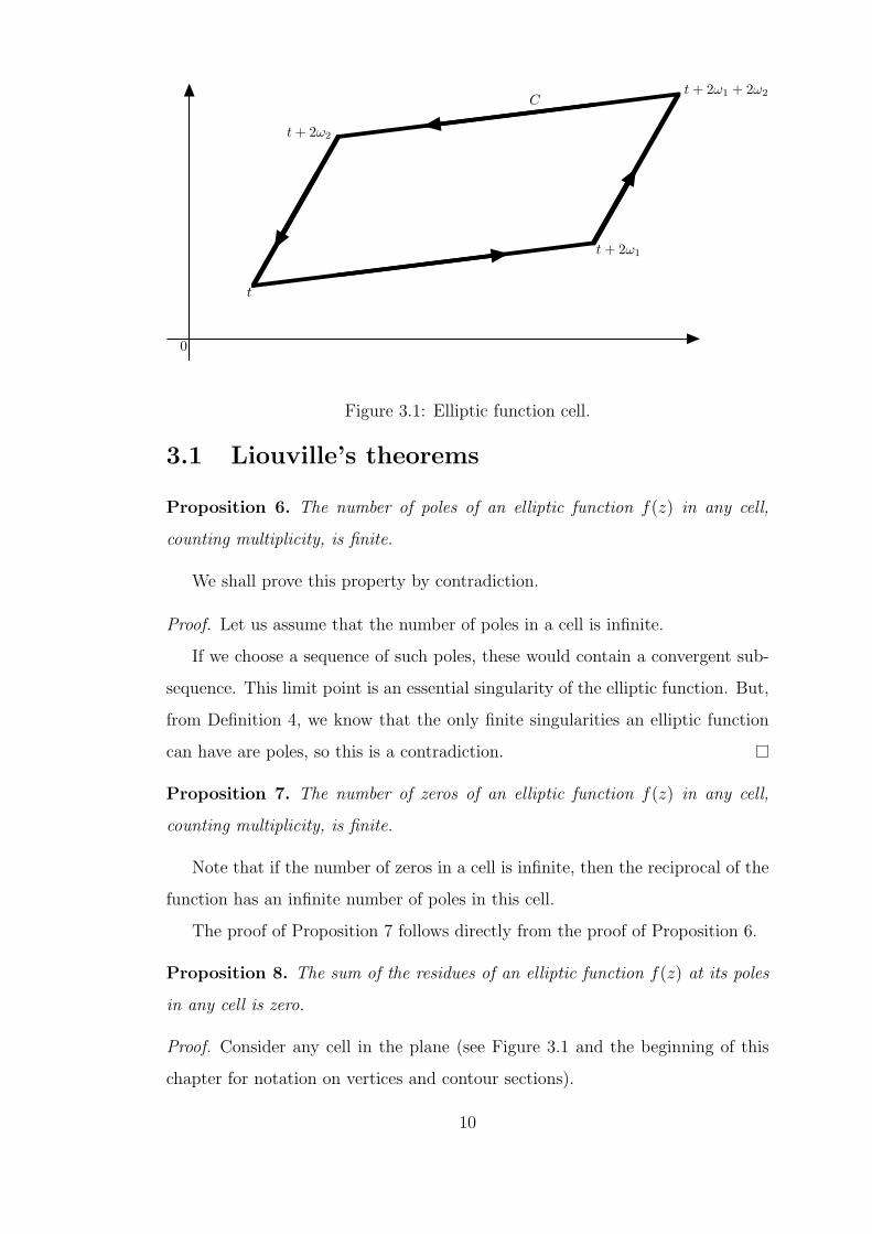
Recall the concept of a mesh in §2.1. In order to integrate this area, we must
translate (without rotation) such a mesh. This is then called a cell (and it has
the same values as any mesh). Figure 3.1 shows a cell with vertices on the points
t, t+2ω1, t+2ω1 +2ω2 and t+2ω2. The contour of the parallelogram constructed
will be denoted by C. This contour can be divided into four sections, starting in
the point t and reaching every vertex in the anticlockwise direction. These will
be denoted by γ1, γ2, γ3 and γ4.
We are going to study some general properties of elliptic functions. Many
textbooks refer to some of these properties as Liouville’s Theorems (for instance,
Akhiezer’s Elements of the theory of elliptic functions [5]) for their relation with
the well-known Liouville’s Theorem:
Theorem 5. Let f(z) be analytic for all z and let | f(z) |< K for all z, where
K is a constant (so that | f(z) | is bounded as | z |→ ∞). Then f(z) is constant.
The main reference used for the study of the following theorems has been [4].
However, [5] and [6] have been invaluable for the understanding of some of the
proofs.
9
0
t
t + 2ω1
t + 2ω2
t + 2ω1 + 2ω2C
Figure 1. The graph repeats after any distance T . The function is determined from any interval T .
1
Figure 3.1: Elliptic function cell.
3.1 Liouville’s theorems
Proposition 6. The number of poles of an elliptic function f(z) in any cell,
counting multiplicity, is finite.
We shall prove this property by contradiction.
Proof. Let us assume that the number of poles in a cell is infinite.
If we choose a sequence of such poles, these would contain a convergent sub-
sequence. This limit point is an essential singularity of the elliptic function. But,
from Definition 4, we know that the only finite singularities an elliptic function
can have are poles, so this is a contradiction.
Proposition 7. The number of zeros of an elliptic function f(z) in any cell,
counting multiplicity, is finite.
Note that if the number of zeros in a cell is infinite, then the reciprocal of the
function has an infinite number of poles in this cell.
The proof of Proposition 7 follows directly from the proof of Proposition 6.
Proposition 8. The sum of the residues of an elliptic function f(z) at its poles
in any cell is zero.
Proof. Consider any cell in the plane (see Figure 3.1 and the beginning of this
chapter for notation on vertices and contour sections).
10
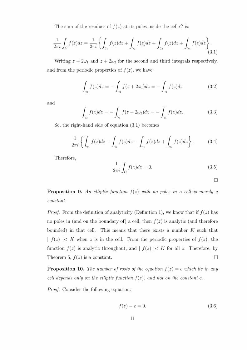
The sum of the residues of f(z) at its poles inside the cell C is:
1
2πi
∫C
f(z)dz =1
2πi
∫γ1
f(z)dz +
∫γ2
f(z)dz +
∫γ3
f(z)dz +
∫γ4
f(z)dz
.
(3.1)
Writing z + 2ω1 and z + 2ω2 for the second and third integrals respectively,
and from the periodic properties of f(z), we have:
∫γ2
f(z)dz = −∫
γ4
f(z + 2ω1)dz = −∫
γ4
f(z)dz (3.2)
and ∫γ3
f(z)dz = −∫
γ1
f(z + 2ω2)dz = −∫
γ1
f(z)dz. (3.3)
So, the right-hand side of equation (3.1) becomes
1
2πi
∫γ1
f(z)dz −∫
γ4
f(z)dz −∫
γ1
f(z)dz +
∫γ4
f(z)dz
. (3.4)
Therefore,1
2πi
∫C
f(z)dz = 0. (3.5)
Proposition 9. An elliptic function f(z) with no poles in a cell is merely a
constant.
Proof. From the definition of analyticity (Definition 1), we know that if f(z) has
no poles in (and on the boundary of) a cell, then f(z) is analytic (and therefore
bounded) in that cell. This means that there exists a number K such that
| f(z) |< K when z is in the cell. From the periodic properties of f(z), the
function f(z) is analytic throughout, and | f(z) |< K for all z. Therefore, by
Theorem 5, f(z) is a constant.
Proposition 10. The number of roots of the equation f(z) = c which lie in any
cell depends only on the elliptic function f(z), and not on the constant c.
Proof. Consider the following equation:
f(z)− c = 0. (3.6)
11

The difference between the number of zeros and the number of poles, which
lie in the cell C, of equation (3.6) is
1
2πi
∫C
f ′(z)
f(z)− cdz. (3.7)
Since 2ω1 and 2ω2 are the periods of the elliptic function f(z),
f ′(z + 2ω1) = f ′(z + 2ω2) = f ′(z). (3.8)
Hence, the integrand in (3.7) is again an elliptic function with the periods 2ω1
and 2ω2.
It follows from the proof of Proposition 8, that the integral (3.7) is equal to
zero. Since the difference between the number of zeros and the number of poles
of equation (3.6) is zero, the number of zeros is in fact equal to the number of
poles. But any pole of equation (3.6) is a pole of f(z) and so the number of zeros
of f(z) − c is equal to the number of poles of f(z), which is independent of the
constant c.
This number is called the order of the elliptic function and is equal to the
number of poles of f(z) in the cell.
Proposition 11. The sum of the affixes of a set of irreducible zeros of an elliptic
function is congruent to the sum of the affixes of a set of irreducible poles.
To prove this proposition we must show that:
Σ affixes of zeros− Σ affixes of poles = period.
Proof. With the division of contour C as in the proof of Proposition 8, we know
12
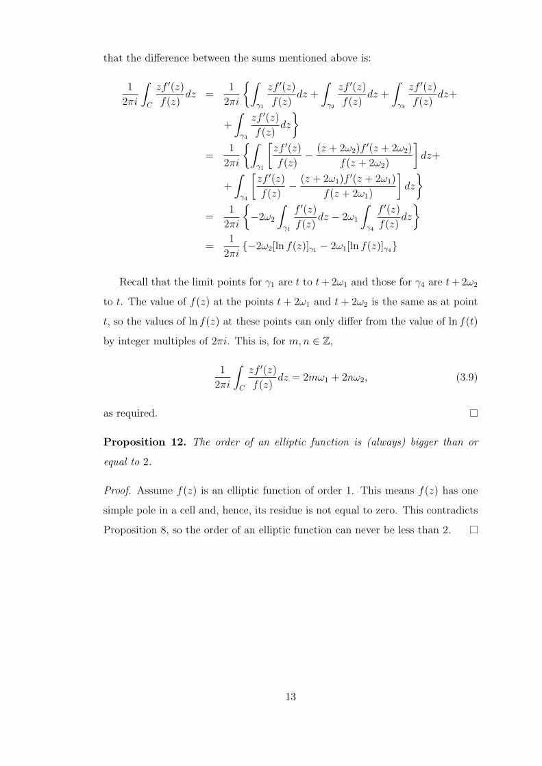
that the difference between the sums mentioned above is:
1
2πi
∫C
zf ′(z)
f(z)dz =
1
2πi
∫γ1
zf ′(z)
f(z)dz +
∫γ2
zf ′(z)
f(z)dz +
∫γ3
zf ′(z)
f(z)dz+
+
∫γ4
zf ′(z)
f(z)dz
=
1
2πi
∫γ1
[zf ′(z)
f(z)− (z + 2ω2)f
′(z + 2ω2)
f(z + 2ω2)
]dz+
+
∫γ4
[zf ′(z)
f(z)− (z + 2ω1)f
′(z + 2ω1)
f(z + 2ω1)
]dz
=
1
2πi
−2ω2
∫γ1
f ′(z)
f(z)dz − 2ω1
∫γ4
f ′(z)
f(z)dz
=
1
2πi−2ω2[ln f(z)]γ1 − 2ω1[ln f(z)]γ4
Recall that the limit points for γ1 are t to t+ 2ω1 and those for γ4 are t+ 2ω2
to t. The value of f(z) at the points t+ 2ω1 and t+ 2ω2 is the same as at point
t, so the values of ln f(z) at these points can only differ from the value of ln f(t)
by integer multiples of 2πi. This is, for m,n ∈ Z,
1
2πi
∫C
zf ′(z)
f(z)dz = 2mω1 + 2nω2, (3.9)
as required.
Proposition 12. The order of an elliptic function is (always) bigger than or
equal to 2.
Proof. Assume f(z) is an elliptic function of order 1. This means f(z) has one
simple pole in a cell and, hence, its residue is not equal to zero. This contradicts
Proposition 8, so the order of an elliptic function can never be less than 2.
13

Chapter 4
Weierstrass functions
The simplest (non-trivial) elliptic functions are of order two. Carl G. J. Jacobi
(1804-1851) chose a function with two simple poles as the standard function of
order two. On the other hand, Karl T. W. Weierstrass (1815-1897) selected one
with a double pole [7].
For the study of Jacobian elliptic functions, we can refer to books such as
Morse and Feshbach’s Methods of theoretical physics [3] or Lawden’s Elliptic func-
tions and applications [8].
Here, we are going to discuss Weierstrassian elliptic functions; in particular,
his ℘ function.
4.1 The Weierstrass ℘ function
The Weierstrass ℘ function is an elliptic function with one second-order pole and
two zeros per unit cell [3].
It is easy to think of the simplest function with one second-order pole; this is,
f(z) = z−2. But this, by itself, does not constitute an elliptic function, for it has
no periods.
The Weierstrass ℘ function is defined
℘(z) =1
z2+
∑m,n
′[
1
(z − 2mω1 − 2nω2)2− 1
(2mω1 + 2nω2)2
], (4.1)
where the symbol Σ′ means that the summation is made over all combinations
14

Figure 4.1: Weierstrass ℘(z) function in absolute value.
of integers m and n except for the combination m = n = 0; 2ω1 and 2ω2 are
the periods of the function ℘ [9]. Figure 4.1 shows a particular ℘(z) function in
absolute value in the form ℘(z, g2, g3).
We will show that ℘(z + 2mω1 + 2nω2) = ℘(z) in the section that follows.
4.1.1 Properties
Theorem 13. The function ℘(z) is an elliptic function with the periods 2ω1, 2ω2.
Its poles are given by z = 2mω1 + 2nω2. It has the further properties:
(i) the principal part of ℘(z) at z = 0 is 1z2 ;
15

(ii) limz→0
(℘(z)− 1z2 ) = 0;
(iii) ℘(z) = ℘(−z);
(iv) ℘′(−z) = −℘′(z) [10].
Proof. (i) and (ii) follow directly from (4.1).
Now note that
℘(−z) =1
z2+
∑m,n
′[
1
(z + Ωm,n)2− 1
(Ωm,n)2
], (4.2)
where Ωm,n = 2mω1 + 2nω2.
The set of points −Ωm,n is the same as the set Ωm,n, which means that the
terms of ℘(−z) are the same as the terms of ℘(z) but in a different order. But
the series for ℘(z) is absolutely convergent, so the disorder of the terms does not
affect the summation of these. Therefore, (iii) holds.
Similarly, consider
℘′(z) =d
dz℘(z) = −2
∑m,n
1
(z − Ωm,n)3. (4.3)
Term-by-term differentiation is permitted since the series for ℘(z) is a uniformly
convergent one of analytic functions. Consider at the same time
℘′(−z) = 2∑m,n
1
(z + Ωm,n)3. (4.4)
We know that the terms of ℘′(−z) are the same as of −℘′(z) but in a different
order because, as before, the sets of points −Ωm,n and Ωm,n are equal. Also, the
sum is not affected either by the derangement of its terms, since the series for
℘′(z) is absolutely convergent [4]. So, (iv) holds too.
Now observe the following:
℘′(z + 2ω1) = −2∑m,n
1
(z − Ωm,n + 2ω1)3. (4.5)
The set of points Ωm,n− 2ω1 is the same as Ωm,n, so the series for ℘′(z+2ω1) is a
16
disorder of the series for ℘′(z). Then, from the fact that this series is absolutely
convergent,
℘′(z + 2ω1) = ℘′(z), (4.6)
meaning that ℘′(z) has period 2ω1.
Similarly, ℘′(z) has period 2ω2.
Integrating equation (4.6):
℘(z + 2ω1) = ℘(z) + C, (4.7)
where C is a constant of integration. Set z = −ω1, then (4.7) becomes:
℘(−ω1 + 2ω1) = ℘(ω1) = ℘(−ω1) + C. (4.8)
From (iii), ℘(ω1) = ℘(−ω1), so C = 0. Therefore,
℘(z + 2ω1) = ℘(z),
and similarly,
℘(z + 2ω2) = ℘(z).
So ℘(z) has periods 2ω1 and 2ω2.
This concludes the proof.
4.2 The differential equation satisfied by ℘(z)
Theorem 14. The elliptic function ℘(z) satisfies the differential equation
℘′2(z) = 4℘3(z)− g2℘(z)− g3, (4.9)
where
g2 = 60∑m,n
′Ω−4
m,n, g3 = 140∑m,n
′Ω−6
m,n
and Ωm,n = 2mω1 + 2nω2 [10].
17

The main reference for the proof of this theorem is Whittaker and Watson’s
A course of modern analysis [4].
Proof. From the definition of the Weierstrass ℘ function (4.1),
℘(z)− 1
z2=
∑m,n
′[
1
(z − 2mω1 − 2nω2)2− 1
(2mω1 + 2nω2)2
], (4.10)
which is even and analytic in a region of which the origin is an internal point.
Using Taylor’s expansions we obtain:
℘(z)− 1
z2=
1
20g2z
2 +1
28g3z
4 + higher order terms, (4.11)
valid for sufficiently small values of | z | and where g2 and g3 have been set to
60∑
m,n′Ω−4
m,n and 140∑
m,n′Ω−6
m,n respectively.
Rearranging for ℘(z) equation (4.11) and differentiating,
℘′(z) = −21
z3+
1
10g2z +
1
7g3z
3 + higher order terms. (4.12)
Now we can cube equation (4.11) and square equation (4.12) to obtain:
℘3(z) =1
z6+
3
20g2
1
z2+
3
28g3 + higher order terms (4.13)
and
℘′2(z) = 4
1
z6− 2
5g2
1
z2− 4
7g3 + higher order terms (4.14)
respectively.
Next subtract four times equation (4.13) of equation (4.14):
℘′2(z)− 4℘3(z) = −g2
1
z2− g3 + higher order terms. (4.15)
If you substitute 1z2 for ℘(z) in this last equation, you will get the following
function:
℘′2(z)− 4℘3(z) + g2℘(z) + g3 = higher order terms. (4.16)
This function is an elliptic function analytic at the origin and, thus, analytic
18

at all congruent points. But these points are the only possible singularities, so
this elliptic function has no singularities and hence, by Proposition 9, the function
is a constant.
Making z tend to zero, so as to see what will become of the right-hand side
of (4.16), shows that this constant is in fact zero.
Therefore ℘(z) satisfies the differential equation
℘′2(z) = 4℘3(z)− g2℘(z)− g3,
where the invariants g2 and g3 are as follows:
g2 = 60∑m,n
′Ω−4
m,n and g3 = 140∑m,n
′Ω−6
m,n.
4.2.1 Converse proof
Alternatively, one may be given
(dy
dx
)2
= 4y3 − g2y − g3. (4.17)
If two numbers ω1 and ω2 can be determined such that
g2 = 60∑m,n
′Ω−4
m,n and g3 = 140∑m,n
′Ω−6
m,n,
then the general solution of the differential equation (4.17) is
y = ℘(±z + α), (4.18)
where α is the constant of integration.
Since the Weierstrass ℘(z) function is even,
y = ℘(z ± α), (4.19)
19

and so, without loss of generality, the solution to the equation is
y = ℘(z + α). (4.20)
20
Chapter 5
The constants e1, e2, e3
We are now going to relate the Weierstrass ℘ function to the constants e1, e2 and
e3 [4] by showing that:
• ℘(ω1), ℘(ω2) and ℘(ω3), where ω3 = −ω1 − ω2, are all unequal; and
• if ℘(ω1) = e1, ℘(ω2) = e2 and ℘(ω3) = e3 then the constants e1, e2 and e3
are the roots of the elliptic curve 4t3 − g2t− g3 = 0, where g2 and g3 are as
in §4.2.
5.1 ℘(ω1), ℘(ω2), ℘(ω3)
First consider ℘′(ω1). From the oddity of the derivative of the Weierstrass ℘
function, we know
℘′(ω1) = −℘′(−ω1).
On the other hand, from its periodic properties,
−℘′(−ω1) = −℘′(2ω1 − ω1) = −℘′(ω1).
But ℘′(ω1) 6= −℘′(ω1) since we already established that ℘′(z) is not even, but
odd. Hence, ℘′(ω1) = 0.
Similarly,
℘′(ω2) = −℘′(−ω2) = −℘′(2ω2 − ω2) = −℘′(ω2),
21

so ℘′(ω2) = 0; and
℘′(ω3) = ℘′(−ω1 − ω2)
= −℘′(ω1 + ω2)
= −℘′(ω1 + ω2 − 2ω1 − 2ω2)
= −℘′(−ω1 − ω2)
= −℘′(ω3),
so ℘′(ω3) = 0.
Now,
℘′(z) = −2∑m,n
1
(z − 2mω1 − 2nω2)3.
From this, it is easy to see that ℘′(z) has poles of order three at the points
congruent to the origin (these make the denominator in the summation zero, so
the function blows up) as its only singularities. Then, from Proposition 11, ℘′(z)
has (only) three irreducible zeros, and so, the only zeros of ℘′(z) are the points
congruent to ω1, ω2 and ω3.
Now consider the function ℘(z) = e1. The function vanishes at z = ω1 and,
since ℘′(ω1) = 0, it has a double zero at z = ω1. Since ℘(z) is an elliptic function
of order 2, it only has two irreducible poles, which implies that the only zeros
of ℘(z) = e1 are congruent to w1. Similarly, the only zeros of ℘(z) = e2 and of
℘(z) = e3 are double zeros at points congruent to ω2 and ω3 respectively.
Observe that if e1 = e2 then ℘(z) = e1 has a zero at ω2 which is a point not
congruent to ω1, so e1 6= e2. If e1 = e3 then ℘(z) = e1 has a zero at ω3 which is
again a contradiction, so e1 6= e3. And finally, if e2 = e3 then ℘(z) = e2 has a
zero at ω3 which is not a point congruent to ω2, so e2 6= e3. So e1, e2 and e3 are
all distinct.
Therefore, ℘(ω1), ℘(ω2) and ℘(ω3), where ω3 = −ω1 − ω2, are all distinct.
22

5.2 e1, e2, e3 and the curve 4t3 − g2t− g3 = 0
In §4.2 we saw the differential equation satisfied by ℘(z) (equation (4.9)):
℘′2(z) = 4℘3(z)− g2℘(z)− g3.
Also, we just discussed that ℘′(z) vanishes at z = ω1, ω2 and ω3 (§5.1).
From these two remarks, it follows that 4℘3(z) − g2℘(z) − g3 vanishes when
℘(z) = e1, e2 or e3. This means that the constants e1, e2 and e3 are the roots of
the elliptic curve
4t3 − g2t− g3 = 0
with g2 and g3 as before, and from the formulae connecting the roots of equations
with their coefficients, we have:
(i) e1 + e2 + e3 = 0;
(ii) e2e3 + e3e1 + e1e2 = −14g2; and
(iii) e1e2e3 = 14g3.
23

Chapter 6
Representation of elliptic
functions in terms of ℘ and ℘′
Theorem 15. Any elliptic function f(z) can be expressed in terms of the Weier-
strassian elliptic functions ℘(z) and ℘′(z) with the same periods, the expression
being rational in ℘(z) and linear in ℘′(z) [4].
This is to say, f(z) may be written as:
f(z) = R1[℘(z)] +R2[℘(z)]℘′(z)
where R1 and R2 are two rational functions.
Next, we shall see how this theorem is obtained.
6.1 The proof
First, let f(z) be any elliptic function and ℘(z) be the Weierstrassian elliptic
function discussed in §4, and let both these functions have the same two periods
2ω1 and 2ω2.
Now, take f(z) to be the following function:
f(z) =1
2[f(z) + f(−z)] +
1
2[f(z)− f(−z)℘′(z)−1]℘′(z). (6.1)
24

We can then say that f(z) is even, and so the functions
f(z) + f(−z) and f(z)− f(−z)℘′(z)−1 (6.2)
are both even functions.
Also, it is clear that if f(z) is an elliptic function, these two functions are
elliptic functions too.
Theorem 15 will be effected if we can express any even elliptic function φ(z),
say, in terms of ℘(z) [4].
If we let a be a zero of φ(z) in any cell, then the point in the cell congruent to
−a is a zero too. From this, the irreducible zeros of φ(z) may be divided into two
sets as follows: a1, a2, ..., an and certain points congruent to −a1,−a2, ...,−an.
Similarly, the irreducible poles of φ(z) may be divided: b1, b2, ..., bn and certain
points congruent to −b1,−b2, ...,−bn.
Consider the function:
1
φ(z)
n∏r=1
℘(z)− ℘(ar)
℘(z)− ℘(br)
. (6.3)
Function (6.3) is an elliptic function of z.
Note that we know the poles and zeros of ℘(z) and the product of function
(6.3) holds the same ones (with same order of multiplicity) as the function φ(z).
Since the latter one is dividing the product, the function has no poles and, by
Proposition 9, is actually a constant.
Thus,
φ(z) = An∏
r=1
℘(z)− ℘(ar)
℘(z)− ℘(br)
, (6.4)
where A is the aforementioned constant.
So we have expressed φ(z) as a rational function of ℘(z).
Applying this same process to each of the functions (6.2) we obtain Theorem
15, as desired.
25

6.2 Application
From the proof of Theorem 15 we can deduce that if we have the poles and zeros
of a function, then we can write the elliptic function using (6.4):
φ(z) = A
n∏r=1
℘(z)− ℘(ar)
℘(z)− ℘(br)
,
where ai and bi are the zeros and the poles of the function, respectively.
Example 16. Construct an elliptic function f(z) with zeros at z = 1± i and poles
at z = 0 and z = i.
Let us check if
f(z) =[℘(z)− ℘(1 + i)][℘(z)− ℘(1− i)]
℘(z)− ℘(i)(6.5)
would be correct.
Observe how, if z = 1 + i then the left multiplier of the numerator becomes
zero, making f(z) = 0, and therefore z = 1 + i is a zero of f(z). Similarly, if
z = 1− i, the right multiplier of the numerator becomes zero, making f(z) = 0,
and so z = 1− i is also a zero of f(z).
To check that 0 and i are poles of f(z), first set z = i. The denominator
becomes zero, so z = i is a pole of f(z). Similarly, consider when z tends to zero.
We know that z = 0 is a pole of ℘(z), since ℘(z) → ∞ as z → 0. When this
occurs, ℘(1 + i), ℘(1− i) and ℘(i) become negligible and we have
℘2(z)
℘(z)= ℘(z),
which tends to infinity as z tends to zero. So z = 0 is also a pole of f(z).
Thus, (6.5) is indeed the elliptic function we were looking for.
26
Chapter 7
Addition theorems
In §6 it was shown that any elliptic function can be expressed in terms of the
Weierstrass ℘(z) function and its derivative. For this reason, when we discuss
theorems in relation to elliptic functions in ℘(z), we know that they apply to all
elliptic functions.
All elliptic functions have addition theorems. In this chapter we aim to study
some forms of these. These theorems show that it is possible to express ℘(u+ v)
in terms of ℘(u), ℘(v) and their derivatives, for general values of u and v [10].
7.1 Addition theorem 1
Theorem 17.
∣∣∣∣∣∣∣∣∣℘(u) ℘′(u) 1
℘(v) ℘′(v) 1
℘(u+ v) −℘′(u+ v) 1
∣∣∣∣∣∣∣∣∣ = 0 [4].
Proof. Consider the following equations:
℘′(u) = A℘(u) +B and ℘′(v) = A℘(v) +B. (7.1)
These equations determine the constants A and B in terms of u and v unless
u ≡ ±v (mod 2ω1, 2ω2) (this is, unless ℘(u) = ℘(v)).
Now consider the function of ξ:
℘′(ξ) = A℘(ξ) +B. (7.2)
27

The function ℘′(ξ) has a triple pole at ξ = 0 and, therefore, by Proposition 11, it
has exactly three irreducible zeros. The sum of these zeros forms a period and,
given that ξ = u and ξ = v are two zeros, the third zero, say ξ = w, is such that
w = −u− v (mod 2ω1, 2ω2).
This implies that w is a zero of the function (7.2), which then gives the
following:
℘′(w) = A℘(w) +B. (7.3)
Eliminating A and B throughout, the discriminant obtained is:∣∣∣∣∣∣∣∣∣℘(u) ℘′(u) 1
℘(v) ℘′(v) 1
℘(−w) −℘′(−w) 1
∣∣∣∣∣∣∣∣∣ = 0,
which implies
℘(u)[℘′(v) +℘′(−w)]−℘′(u)[℘(v)−℘(−w)] + [−℘(v)℘′(−w)−℘′(v)℘(−w)] = 0.
Which, using the oddity of ℘′(z) and evenness of ℘(z) (this is, ℘′(z) = −℘′(−z)
and ℘(z) = ℘(−z)), can be written as
℘(u)℘′(v)− ℘(u)℘′(w)− ℘′(u)℘(v) + ℘′(u)℘(w) + ℘(v)℘′(w)− ℘′(v)℘(w) = 0.
Since this result expresses ℘(u + v) algebraically in terms of ℘(u) and ℘(v),
the Addition Theorem 17 holds, where u+ v = −w.
7.2 Addition theorem 2
Theorem 18. ℘(u+ v) = 14
[℘′(u)−℘′(v)℘(u)−℘(v)
]2
− ℘(u)− ℘(v) [4].
Proof. Consider once more the function (7.2). When ξ is congruent to any of the
zeros ξ = u, ξ = v or ξ = −u− v = w, squaring the function and rearranging it
gives:
℘′2(ξ)− [A℘(ξ) +B]2 = 0.
28

If ℘(ξ) is equal to any of ℘(u), ℘(v) or ℘(−w), then
4℘3(ξ)− A2℘2(ξ)− (2AB + g2)℘(ξ) + (B2 + g3) = 0, (7.4)
where g2 and g3 are as given in §4.2.
℘(u), ℘(v) and ℘(−w) are all unequal for general values of u and v, and so
they are all roots of (7.4).
Consequently, using the formula for the sum of the roots of a cubic equation,
we obtain
℘(u) + ℘(v) + ℘(−w) =1
4A2. (7.5)
By means of rearranging (7.5),
℘(−w) =1
4
[℘′(u)− ℘′(v)
℘(u)− ℘(v)
]2
− ℘(u)− ℘(v),
which, if you substitute w for −u− v, becomes the Addition Theorem 18:
℘(u+ v) =1
4
[℘′(u)− ℘′(v)
℘(u)− ℘(v)
]2
− ℘(u)− ℘(v).
This result expresses explicitly ℘(u + v) in terms of ℘(u), ℘(v) and their
derivatives, as desired.
7.3 Other addition theorems
Many algebraic addition theorems for elliptic functions can be found. Here are
two other such examples.
Example 19. ℘′(u+ v) = ℘(u+v)[℘′(u)−℘′(v)]+℘(u)℘′(v)−℘′(u)℘(v)℘(v)−℘(u)
[7].
Example 20. ℘(u+ v)− ℘(u− v) = −℘′(u)℘′(v)[℘(u)−℘(v)]2
[4].
To prove these, we can account for poles and zeros on the left-hand side of
the identities and check these are the same on the right-hand side (or vice versa),
and confirm that Theorem 5 holds by studying the behaviour of both sides of the
identity at a chosen limiting point.
For instance, Example 20 may be proved in the following way.
29
Proof. Let us assume v is a constant.
Consider first the left-hand side of the identity,
℘(u+ v)− ℘(u− v). (7.6)
z is a zero of (7.6) if (7.6) equals zero when u = z.
• u = 0 ⇒ ℘(0 + v)− ℘(0− v) = ℘(v)− ℘(−v) = ℘(v)− ℘(v) = 0;
• u = ω1 ⇒ ℘(ω1 + y)− ℘(ω1 − y) = ℘(ω1 + y)− ℘(−ω1 + y) = ℘(ω1 + y)−
℘(−ω1 + y + 2ω1) = ℘(ω1 + y)− ℘(ω1 + y) = 0;
and similarly for u = ω2 and u = ω3. So 0, ω1, ω2 and ω3 are all zeros of (7.6).
Let us check these are the zeros of the right-hand side of the identity,
−℘′(u)℘′(v)[℘(u)− ℘(v)]2
. (7.7)
• u = 0 ⇒ −℘′(0)℘′(v)[℘(0)−℘(v)]2
= 0 since ℘′(0) = 0;
• u = ω1 ⇒ −℘′(ω1)℘′(v)[℘(ω1)−℘(v)]2
= 0 since ℘′(ω1) = 0;
and similarly for u = ω2 and u = ω3. So the zeros are the same for both sides of
the identity.
Now let us look for poles. These will be the points that will make both sides
of the identity tend to infinity. In (7.6) we deal with ℘(z). From equation (4.1)
we know that it tends to infinity when z = 0. So (7.6) tends to infinity when
u = ±v. These are double poles, so the number of poles is equal to the number
of zeros, and we are done looking for poles.
Let us confirm u = ±v are also poles of (7.7). The function will tend to
infinity when ℘(u) − ℘(v) is equal to zero. This occurs when u = ±v, and the
square in the denominator makes these double poles.
Finally, let us consider the behaviour of the identity when u tends to zero.
When u→ 0, ℘(u) ∼ z−2 and ℘′(u) ∼ −2z−3.
℘(u+ v) ' ℘(v) + ℘′(v)u+O(u2)
30
and
℘(u− v) = ℘(v − u) ' ℘(v)− ℘′(v)u+O(u2),
so ℘(u+ v)− ℘(u− v) ' 2℘′(v)u. So (7.6) behaves like 2u.
Now, (7.7) behaves like 2z−3
[z−2]2= 2z, so both sides of the identity behave in the
same manner.
Thus it is proved that the addition theorem of Example 20 holds.
31

Chapter 8
The Weierstrass theorem
Definition 3 told us what a meromorphic function is. Now we want to relate these
functions to algebraic addition theorems.
So, a meromorphic function φ(z) has an algebraic addition theorem if there
exists an identity
F (φ(z1 + z2), φ(z1), φ(z2)) = 0, (8.1)
where F is an entire rational function of its arguments [5]. From equation (8.1)
we understand that φ(z1 + z2) can be expressed algebraically in terms of φ(z1)
and φ(z2).
In §7 we said that all elliptic functions possess algebraic addition theorems.
These also hold for degeneracies of elliptic functions (this is, their limiting cases),
such as any rational function of z and also any rational function of eiπzω .
The following theorem (given by Weierstrass) states that, in fact, the above
two examples are the only meromorphic functions that have an algebraic addition
theorem.
Theorem 21. Any meromorphic function φ(z) possessing an algebraic addition
theorem is either an elliptic function or is of the form R(z) or R(eλz), where R
is a rational function [11].
Note that in Theorem 21, λ = iπω
.
We will continue to prove Weierstrass’ Theorem with the aid of W. S. Osgood’s
proofs in [5] and [11], after stating a necessary theorem.
32

8.1 Picard’s Theorem
The following theorem is known as the Big Picard Theorem.
Theorem 22. Any analytic function φ(z) assumes in an arbitrary neighbourhood
of an essentially singular point any finite value except, perhaps, one value [11].
So if an entire function omits two (or more) values, then it is a constant.
8.2 The proof
The following is the proof of the Weierstrass Theorem (Theorem 21).
Proof. Suppose that the meromorphic function φ(z) has an algebraic addition
theorem as (8.1). Assume that F (x1, x2, x3) is a polynomial in x1, x2, x3 and, as
a polynomial in x1 (for us, x1 = φ(z1 + z2)), the degree is m. We have to show
that φ(z) is either rational, elliptic or simply periodic. Suppose it is not rational
and thus, z = ∞ is an essential singularity of φ(z).
We choose a C such that φ(z) = C has many solutions (and C is not omitted
by φ(z)). Using the Big Picard Theorem (Theorem 22), we know there are m+1
different solutions to this equation, and we shall denote them by a0, a1, a2, ..., am.
Also, choose a ξ such that ξ, a0 + ξ, a1 + ξ, a2 + ξ, ..., am + ξ are all regular points.
Now consider the following equation:
F (x, φ(z), C) = 0, (8.2)
where z is one of the points ak + ξ (k = 0, 1, 2, ...,m). Setting z1 = z and z2 = ak
in equation (8.1) we get:
F (φ(z + ak), φ(z), φ(ak)) = 0. (8.3)
If we write C = φ(ak) and x = φ(z + ak), we obtain equation (8.2). So (8.2) has
roots for x = φ(z + ak) (k = 0, 1, 2, ...,m). Observe that since k = 0, 1, 2, ...,m,
there are m+ 1 such solutions.
33

Since F (x, φ(z), C) is a polynomial in x of degree m, the roots of x = φ(z+ak)
(k = 0, 1, 2, ...,m) cannot all be distinct, so
φ(z + ar) = φ(z + as) (8.4)
for each z in some neighbourhood of ξ and r = 0, 1, 2, ...,m and s = 0, 1, 2, ...,m
but r 6= s. From this, we can state φ(z) to have period ar−as, which means that
φ(z) is periodic.
If φ(z) is doubly periodic, from the definition of an elliptic function (Definition
4), the theorem is proved. So it remains to be checked what happens if φ(z) is
simply periodic.
For simplicity, assume that the period of φ(z) is equal to 2π. We want to
show that φ(z) = R(ω), where ω = eiz and R represents a rational function. The
map z 7→ ω = eiz sends the strip 0 < R(z) < 2π into the ω-plane, with the
cut from 0 to +∞. We can see that φ(z) = ψ(ω) is meromorphic in the whole
ω-plane and has punctured points at z = 0 and z = ∞. If neither of these points
are essential singularities, then the function ψ(z) is rational. But if we assume
that at least one of these two points is an essential singularity, then we can apply
Theorem 22 once again to find m+1 distinct points bk (k = 0, 1, 2, ...,m) at which
ψ(ω) = C, as before. The inverse images of these b0, b1, b2, ..., bm lie in the strip
0 ≤ R(z) < 2π, showing that φ(z) as presented in equation (8.2) has a period
whose real part is < 2π, which is a contradiction to our initial assumption, that
is that the function φ(z) has a single period of 2π.
Therefore, the Weierstrass Theorem is proved.
34

Chapter 9
Some consequences of ω2 →∞
As a final note for this dissertation, we will study the limits, when ω2 tends to
infinity, of g2, g3 and the Weierstrass ℘(z) function.
9.1 g2∞ and g3∞
Recall from §4.2 that
g2 = 60∑m,n
′ 1
(2mω1 + 2nω2)4
and
g3 = 140∑m,n
′ 1
(2mω1 + 2nω2)6.
Let g2∞ and g3∞ be the limits of g2 and g3 when ω2 tends to infinity, respec-
tively.
35

g2∞ = limω2→∞
g2
= 60∑m6=0
1
(2mω1)4
= 120∞∑
m=1
1
(2mω1)4
=15
2ω41
∞∑m=1
1
m4
=15
2ω41
π4
90
=π4
12ω41
.
g3∞ = limω2→∞
g3
= 140∑m6=0
1
(2mω1)6
= 280∞∑
m=1
1
(2mω1)6
=35
8ω61
∞∑m=1
1
m6
=35
8ω61
π6
945
=π6
216ω61
.
As expected, from the definitions of g2 and g3, letting ω2 tend to infinity
expresses g2∞ and g3∞ only in terms of the remaining period, 2ω1.
They differ by a factor of π2
18ω21. Both g2∞ and g3∞ will tend to zero as ω1 tends
to infinity, but g3∞ will tend to this limit faster.
36
9.2 ℘∞(z)
Let ℘∞(z) be the limit of the Weierstrass ℘(z) function when ω2 tends to infinity.
℘∞(z) = limω2→∞
℘(z)
=1
z2+
∑m6=0
[1
(z − 2mω1)2− 1
(2mω1)2
]
=∑m∈Z
1
(z − 2mω1)2− 1
2ω21
∞∑m=1
1
m2
= − π2
4ω21(−1 + cos( πz
2ω1)2)
− π2
6.
It is interesting to see that making one of the periods of the Weierstrass ℘(z)
function tend to infinity, the expression obtained is one involving the trigonomet-
ric function of cosine with respect to the inverse of the period that is left.
37

Chapter 10
Conclusion
We have then discussed the basic properties of elliptic functions and studied some
interesting theorems and propositions that surround them.
We have learnt about the simplest non-trivial elliptic function, the Weier-
strass ℘(z) function, and how all elliptic functions can be expressed by means
of this particular one. We have also fully proved the Weierstrass Theorem on
meromorphic functions having algebraic addition theorems.
It has been a very analytic paper. For the study of some ”real life” applica-
tions, I recommend the book Elliptic functions and applications by D. F. Lawden
[8].
38

Bibliography
[1] Lang, S. 1973, Elliptic functions, Addison-Wesley Publishing Company, Inc.
[2] Spiegel, M. R. 1971, Variable compleja, McGraw-Hill
[3] Morse, P. M. & Feshbach, H. 1953, Methods of theoretical physics, McGraw-
Hill
[4] Whitakker, E. T., & Watson, G. N. 1996, A course of modern analysis,
Cambridge University Press
[5] Akhiezer, N. I. 1990, Elements of the theory of elliptic functions, American
Mathematical Society
[6] Braden, H. W. 2008, Notes for the course Elliptic curves and applications,
University of Edinburgh
[7] Abramowitz, M. & Stegun, I. A. 1972, Handbook of mathematical functions,
Dover Publications, Inc.
[8] Lawden, D. F. 1989, Elliptic functions and applications, Springer-Verlag
[9] Gradshteyn, I. S. & Ryzhik, I. M. 1981, Table of integrals, series, and prod-
ucts, Academic Press
[10] Chandrasekharan, K. 1985, Elliptic functions, Springer-Verlag
[11] Prasolov, V. & Solovyev, Y. 1997, Elliptic functions and elliptic integrals,
American Mathematical Society
39