ellen r. mcgrattan may 2015 - university of …users.econ.umn.edu/~erm/seminars/euilectures.pdfellen...
TRANSCRIPT

EUI Le tures in Quantitative Ma roe onomi s
Ellen R. McGrattan
May 2015
Materials at ftp.mpls.frb.fed.us/pub/research/mcgrattan

Outline of Lectures
I. Business cycle accounting: Methods and misunderstandings
II. Beyond business cycle accounting: Some applications
III. Back to methods: Nonlinearities and large state spaces

I. BCA: Methods and Misunderstandings

Some Background
• Want preliminary data analysis technique
• Goals:
Isolate promising classes of models/theories/stories
Guide development of theory
Avoid critiques of structural VARs

Idea of Approach
• Equivalence results:
Detailed models with frictions observationally equivalent to
Prototype growth model with time-varying wedges
• Accounting procedure:
Use theory plus data to measure wedges
Estimate stochastic process governing expectations
Feed wedges back one at a time and in combinations
How much of output, investment, labor accounted for by each?

Prototype Growth Model
• Consumption (c), labor (l), investment (x) solve
maxct,lt,xtE∑∞
t=0 βtU(ct, lt)
subject to
ct + (1 + τxt)xt ≤ (1− τlt)wtlt + rtkt + Tt
kt+1 = (1− δ)kt + xt
• Production: yt = AtF (kt, γtlt)
• Resource: ct + gt + xt = yt

Prototype Growth Model
• Consumption (c), labor (l), investment (x) solve
maxct,lt,xtE∑∞
t=0 βtU(ct, lt)
subject to
ct + (1 + τxt)xt ≤ (1− τlt)wtlt + rtkt + Tt
kt+1 = (1− δ)kt + xt
• Production: yt = AtF (kt, γtlt)
• Resource: ct + gt + xt = yt
Note: Time-varying wedges (in red) are not structural

First-order Conditions of Prototype Model
• Efficiency wedge:
yt = AtF (kt, γtlt)
• Labor wedge:
−Ult
Uct
= (1− τlt)(1− α)yt/lt
• Investment wedge:
(1 + τxt)Uct = βEtUct+1 [αyt+1/kt+1 + (1 + τxt+1)(1− δ)]
• Government consumption wedge:
ct + gt + xt = yt

First-order Conditions of Prototype Model
• Efficiency wedge:
yt = AtF (kt, γtlt)
• Labor wedge:
−Ult
Uct
= (1− τlt)(1− α)yt/lt
• Investment wedge:
(1 + τxt)Uct = βEtUct+1 [αyt+1/kt+1 + (1 + τxt+1)(1− δ)]
• Government consumption wedge:
ct + gt + xt = yt
Next, consider mappings between this and other models

Mapping Between Original and Prototype Models
1- l A
1+ x
Sticky wagesUnionsSearch
Inefficient work rules
Agency costsCollateral constraints
Staggered wagesInput financing frictionsIntangible investment
g
Sudden stops

Mapping Between Original and Prototype Models
1- l A
1+ x
Sticky wagesUnionsSearch
Inefficient work rules
Agency costsCollateral constraints
Staggered wagesInput financing frictionsIntangible investment
g
Sudden stops

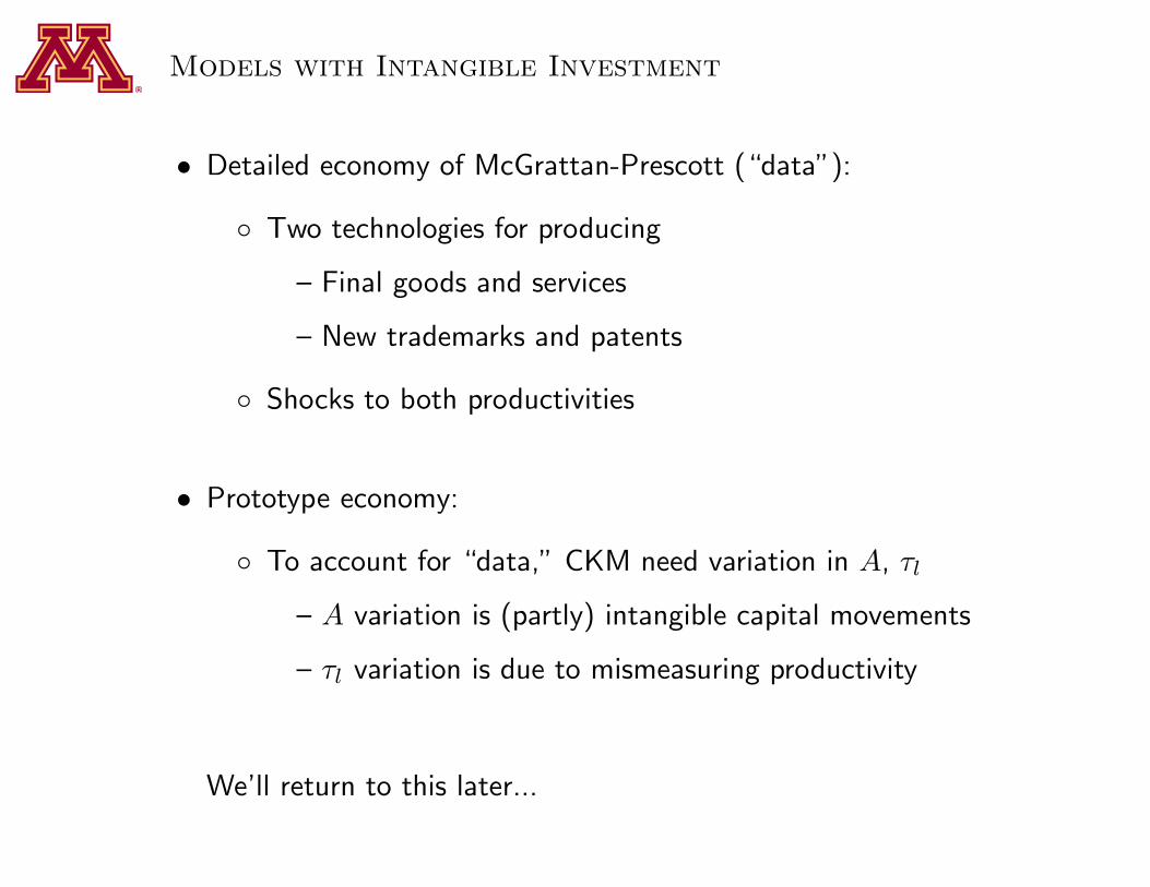
Models with Intangible Investment
• Detailed economy of McGrattan-Prescott (“data”):
Two technologies for producing
– Final goods and services
– New trademarks and patents
Shocks to both productivities
• Prototype economy:
To account for “data,” CKM need variation in A, τl
– A variation is (partly) intangible capital movements
– τl variation is due to mismeasuring productivity
We’ll return to this later...

Measuring Wedges
• Stochastic Process for wedges st = [logAt, τlt, τxt, log gt]
st+1 = P0 + Pst +Qηt+1
• Preferences and technology
U(c, l) = log c+ ψ log(1− l)
F (k, l) = Akθl1−θ
• With data from national accounts
Fix parameters of technology and preferences
Compute MLE estimates of P0, P , Q

Recovering Wedges
• Model decision rules are y(st, kt), x(st, kt), l(st, kt)
• Set:
y(st, kt) = yDATAt
x(st, kt) = xDATAt
l(st, kt) = lDATAt
g(st, kt) = gDATAt
with kt defined recursively from accumulation equation
• Solve for values of st = [logAt, τlt, τxt, log gt]
• Inputting these values gives exactly same series as in data

Main result for US Episodes
• Investment wedge plays small role in
Great Depression
Post WWII business cycles
⇒ Implies many existing theories not promising, e.g.,
Models with agency costs
Models with collateral constraints

Wedges for US Great Depression
1929 1930 1931 1932 1933 1934 1935 1936 1937 1938 193960
70
80
90
100
110
120
US Output
Efficiency wedge
Labor wedge
Investment wedge

Predicted Output without Investment Wedge
1929 1930 1931 1932 1933 1934 1935 1936 1937 1938 193950
60
70
80
90
100
US Output
Model, No investment wedge

Predicted Hours without Investment Wedge
1929 1930 1931 1932 1933 1934 1935 1936 1937 1938 193960
70
80
90
100
US Hours
Model, No investment wedge

Wedges for US 1980s Recession
90
92
94
96
98
100
102
104
106
108
110
US Output
1979 1980 1981 1982 1983 1984 1985
Efficiency wedge
Labor wedge
Investment wedge
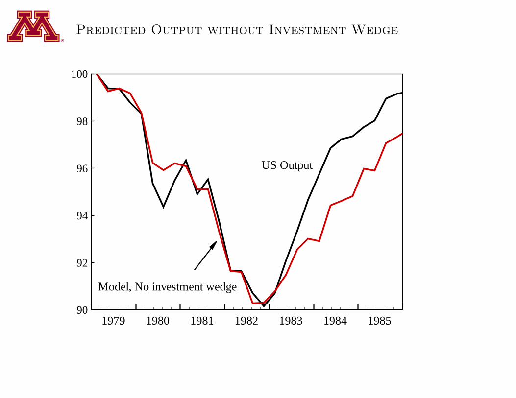
Predicted Output without Investment Wedge
90
92
94
96
98
100
US Output
1979 1980 1981 1982 1983 1984 1985
Model, No investment wedge

Predicted Hours without Investment Wedge
92
94
96
98
100
102
104
US Hours
1979 1980 1981 1982 1983 1984 1985
Model, No investment wedge

Christiano and Davis Critiques of BCA

Critique 1: Results Sensitive to Capital Tax Choice
• Original budget constraint with wedge τxt
ct + (1 + τxt)xt ≤ (1− τlt)wtlt + rtkt + Tt
• Alternative budget constraint with wedge τkt
ct + kt+1 − kt ≤ (1− τlt)wtlt + (1− τkt)(rt − δ)kt + Tt
• Christiano-Davis claim: results sensitive to choice of τxt, τkt
Are they right?

Critique 1: Results Sensitive to Capital Tax Choice
• Original budget constraint with wedge τxt
ct + (1 + τxt)xt ≤ (1− τlt)wtlt + rtkt + Tt
• Alternative budget constraint with wedge τkt
ct + kt+1 − kt ≤ (1− τlt)wtlt + (1− τkt)(rt − δ)kt + Tt
• Christiano-Davis claim: results sensitive to choice of τxt, τkt
Are they right? No!

CKM Response (Fed Staff Report 384)
• Theoretically, the two economies are equivalent
• Numerically,
Can differ slightly if FOCs linearized
But find tiny difference even with extreme adjustment costs

Nearly-Equivalent Model Predictions
90
92
94
96
98
100
102
US Output
Model, with x wedge
1979 1980 1981 1982 1983 1984 1985
Model, with k wedge

CKM Response (Fed Staff Report 384)
• Theoretically, the two economies are equivalent
• Numerically,
Can differ slightly if FOCs linearized
But find tiny difference even with extreme adjustment costs
• Why did CD find a difference?

CKM Response (Fed Staff Report 384)
• Theoretically, the two economies are equivalent
• Numerically,
Can differ slightly if FOCs linearized
But find tiny difference even with extreme adjustment costs
• Why did CD find a difference?
Answer: they didn’t fix expectations

Need to Keep Expectations Fixed
• Let st = [s1t, s2t, s3t, s4t] be latent state vector
st+1 = P0 + Pst +Qǫt+1
• In practice, associate wedges with elements of st:
logA(st) = s1t, τl(st) = s2t, τx(s
t) = s3t, log g(st) = s4t
• For one-wedge contribution, say, of efficiency wedge:
logA(st) = s1t, τl(st) = τl, τx(s
t) = τx, log g(st) = log g

Need Theoretically-Consistent Expectations
90
92
94
96
98
100
102
US Output
1979 1980 1981 1982 1983 1984 1985
Prediction Using a Theoretically-Consistent Methodology (CKM, 2007)
Prediction Using anAlternative Methodology(Christiano-Davis, 2006)

Critique 2: BCA Ignores “Spillover Effects”
• CD use VAR approach
Find financial friction shock important for business cycles
Argue the finding is inconsistent with BCA results
• CKM use BCA approach
Find investment wedge plays small role for business cycles
Argue that CD finding is consistent with BCA results
• How can it be consistent?
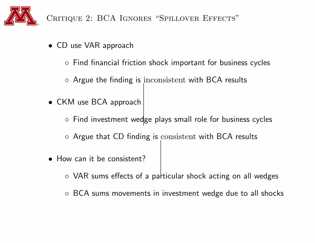
VAR sums effects of a particular shock acting on all wedges
BCA sums movements in investment wedge due to all shocks

Popular Alternative to BCA: Stru tural VARs

Current Practice: Structural VARs
• Provide summaries of facts to guide theorists, e.g.,
What happens after a technology shock?
What happens after a monetary shock?
• Impulse responses used to identify promising classes of models, e.g.,
If SVAR finds positive technology shock leads to fall in hours
Points to sticky price models (not RBC models) as promising
• SVARs are used a lot . . . but are they useful guides for theory?

An Evaluation of SVARs Using Growth Model
• Use prototype growth model
• Plot theoretical impulse response from model
• Generate data from model and apply SVAR procedure
• Plot empirical impulse response identified by SVAR procedure
• Compare responses

Main Findings for SVAR Study
• Using growth model with SVAR assumptions met
• Asking, What happens after technology shock?
• Find:
SVAR procedure does not uncover model’s impulse response
Having capital in model requires infeasibly many VAR lags
Earlier equivalence results imply that SVARs are not useful guides

What You Get from SVAR Procedure
• Structural MA
Xt = A0ǫt +A1ǫt−1 + A2ǫt−2 + . . . , Eǫtǫ′t = Σ

What You Get from SVAR Procedure
• Structural MA for ǫ=[‘technology shock’, ‘demand shock’]′
Xt = A0ǫt +A1ǫt−1 + A2ǫt−2 + . . . , Eǫtǫ′t = Σ
where Xt = [∆ Log labor productivity, (1− αL)Log hours]′
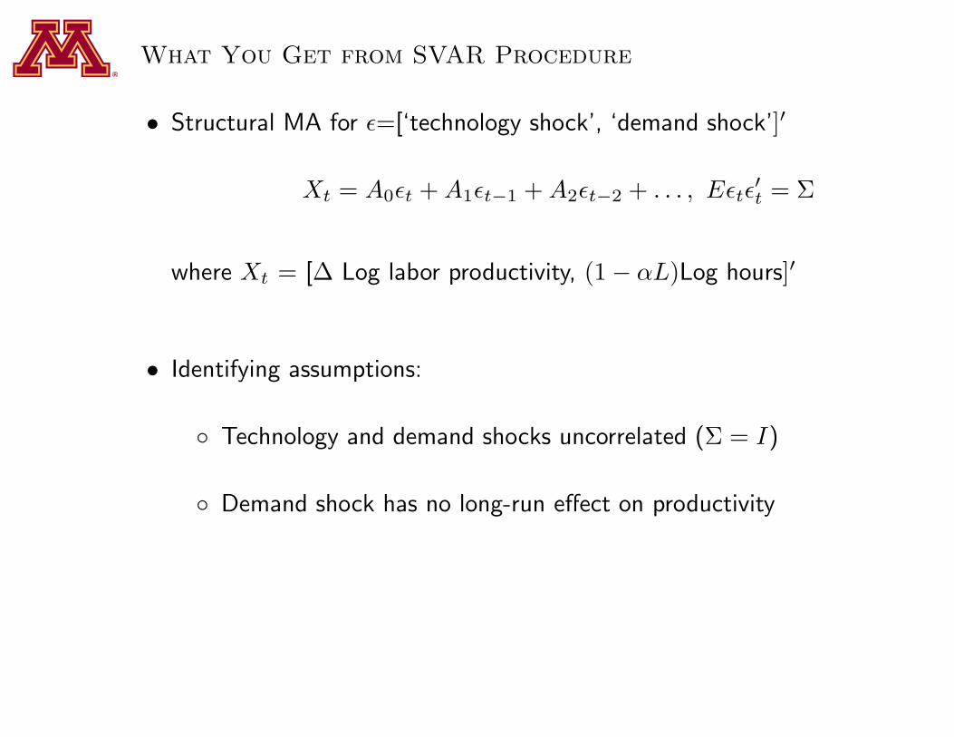
What You Get from SVAR Procedure
• Structural MA for ǫ=[‘technology shock’, ‘demand shock’]′
Xt = A0ǫt +A1ǫt−1 + A2ǫt−2 + . . . , Eǫtǫ′t = Σ
where Xt = [∆ Log labor productivity, (1− αL)Log hours]′
• Identifying assumptions:
Technology and demand shocks uncorrelated (Σ = I)
Demand shock has no long-run effect on productivity

Impulse Responses and Long-Run Restriction
• Impulse response from structural MA:
Blip ǫd1 for response of productivity to demand
log(y1/l1)− log(y0/l0) = A0(1, 2)
log(y2/l2)− log(y0/l0) = A0(1, 2) + A1(1, 2)...
log(yt/lt)− log(y0/l0) = A0(1, 2) +A1(1, 2) + . . .+At(1, 2)
• Long-run restriction:
Demand shock has no long run effect on level of productivity
∑∞j=0Aj(1, 2) = 0

Deriving Structural MA from VAR
• OLS regressions on bivariate VAR: B(L)Xt = vt
Xt = B1Xt−1 +B2Xt−2 + B3Xt−3 +B4Xt−4 + vt, Evtv′t = Ω

Deriving Structural MA from VAR
• OLS regressions on bivariate VAR: B(L)Xt = vt
Xt = B1Xt−1 +B2Xt−2 + B3Xt−3 +B4Xt−4 + vt, Evtv′t = Ω
• Invert to get MA: Xt = B(L)−1vt = C(L)vt
Xt = vt + C1vt−1 + C2vt−2 + . . .
with Cj = B1Cj−1 +B2Cj−2 + . . .+ Bj , j = 1, 2, . . .

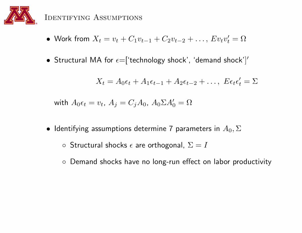
Identifying Assumptions
• Work from Xt = vt + C1vt−1 + C2vt−2 + . . . , Evtv′t = Ω

Identifying Assumptions
• Work from Xt = vt + C1vt−1 + C2vt−2 + . . . , Evtv′t = Ω
• Structural MA for ǫ=[‘technology shock’, ‘demand shock’]′
Xt = A0ǫt +A1ǫt−1 + A2ǫt−2 + . . . , Eǫtǫ′t = Σ
with A0ǫt = vt, Aj = CjA0, A0ΣA′0 = Ω
Identifying Assumptions
• Work from Xt = vt + C1vt−1 + C2vt−2 + . . . , Evtv′t = Ω
• Structural MA for ǫ=[‘technology shock’, ‘demand shock’]′
Xt = A0ǫt +A1ǫt−1 + A2ǫt−2 + . . . , Eǫtǫ′t = Σ
with A0ǫt = vt, Aj = CjA0, A0ΣA′0 = Ω
• Identifying assumptions determine 7 parameters in A0,Σ
Structural shocks ǫ are orthogonal, Σ = I
Demand shocks have no long-run effect on labor productivity
⇒ 7 equations (A0ΣA′0 = Ω, Σ = I ,
∑
j Aj(1, 2) = 0)

Use Growth Model Satisfying 3 Key SVAR Assumptions
• Only 2 shocks (“technology,” “demand”)
• Shocks are orthogonal
• Technology shock has unit root, demand shock does not
This is the best case scenario for SVARs

Specification of Shocks in the Model
• Technology shock is efficiency wedge A = z1−θ
log zt = µz + log zt−1 + ηzt
• “Demand” shock is labor wedge
τlt = (1− ρ)τl + ρτlt−1 + ητt
• With 3 key SVAR assumptions imposed
Only 2 shocks (“technology,” “demand”)
Shocks orthogonal (ηz ⊥ ητ )
Technology shock has unit root, demand shock does not

Our Evaluation of SVAR Procedure
• Use growth model satisfying SVAR’s 3 key assumptions
• Model has theoretical impulse response
Xt = D(L)ηt
• Generate many sequences of data from model
• Apply SVAR to these data to get empirical impulse response
Xt = A(L)ǫt
• Compare model impulse responses with SVAR responses

Three Possible Problems
1. Noninvertibility when α = 1
2. Small samples (around 250 quarters)
3. Short lag length
#3 is quantitatively most important

The Short Lag Length Problem
• Using
Quasi-differencing (QDSVAR) to avoid invertibility problem
100,000 length sample to avoid small sample problem
... still cannot uncover model’s impulse response

Theoretical and Empirical Impulse Responses
Quarter Following Shock
0 10 20 30 40 50 60-0.5
-0.25
0
0.25
0.5
0.75
p=4
p=10
p=20
p=30
Model Impulse Response
QDSVAR Impulse Responses (dashed lines)
p=50
p=100

Long AR Needed Because of Capital
• Capital decision rule, with kt = kt/zt−1:
log kt+1 = γk log kt + γzηzt + γτ τt
• So others, like lt, have ARMA representation
log lt = γk log lt−1 + φz(1− κzL)ηzt + φτ (1− κτL)τt
• What does the AR representation, B(L)Xt = vt, look like?

Model Has Infinite-order AR
• Proposition: Model has VAR coefficients Bj such that
Bj =MBj−1, j ≥ 2,
where M has eigenvalues equal to α (the differencing parameter) and
(γk − γlφk/φl − θ
1− θ
)
γk, γl are coefficients in the capital decision rule
φk, φl are coefficients in the labor decision rule
• Eigenvalues of M are α and .97 for the baseline parameters
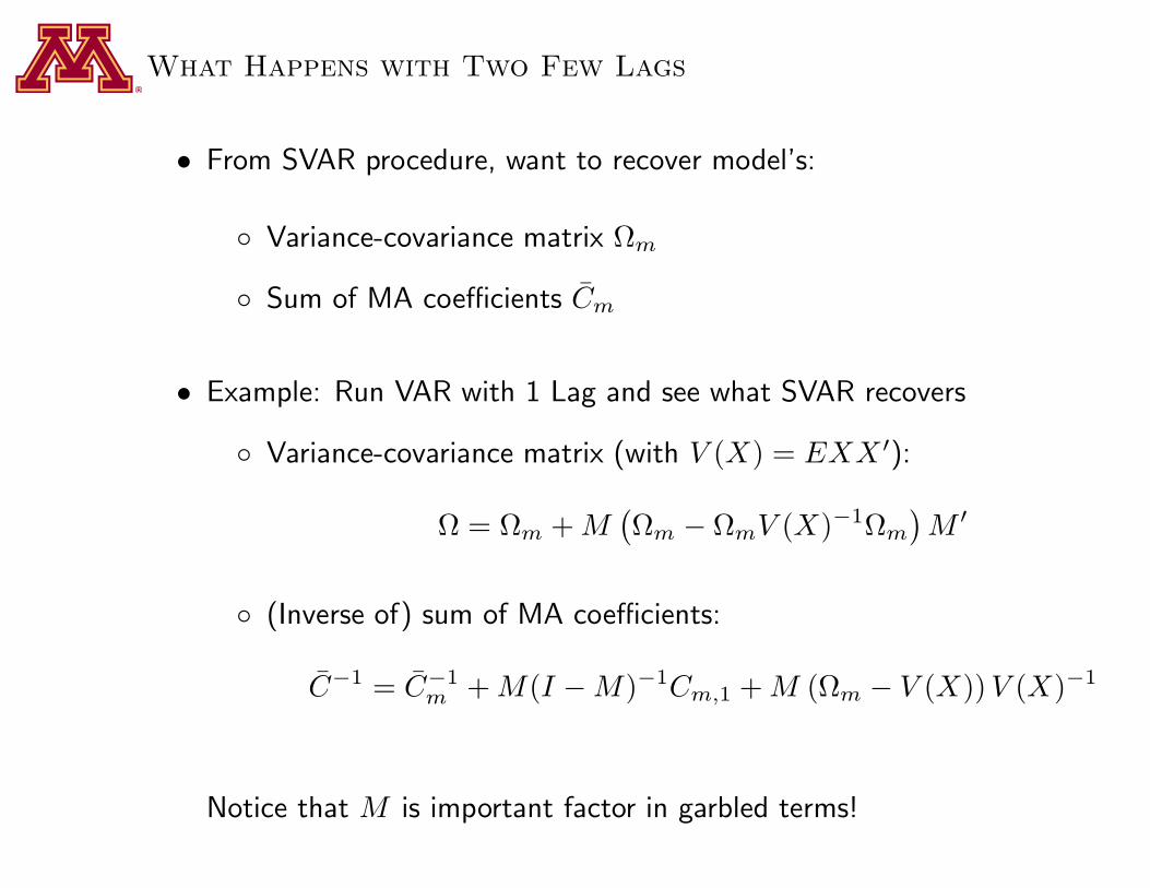
What Happens with Two Few Lags
• From SVAR procedure, want to recover model’s:
Variance-covariance matrix Ωm
Sum of MA coefficients Cm
• Example: Run VAR with 1 Lag and see what SVAR recovers
Variance-covariance matrix (with V (X) = EXX ′):
Ω = Ωm +M(Ωm − ΩmV (X)−1Ωm
)M ′
(Inverse of) sum of MA coefficients:
C−1 = C−1m +M(I −M)−1Cm,1 +M (Ωm − V (X))V (X)−1
Notice that M is important factor in garbled terms!

Problems Still Arise if Hours in Levels
Quarter Following Shock
0 10 20 30 40 50 600
0.25
0.5
0.75
1p=4
p=10
p=20
p=30
p=50
Model Impulse Response
LSVAR Impulse Responses (dashed lines)
p=100

Recap of Lecture I
• BCA is a promising alternative to SVARs
• Statistical methods must be guided by theory
• Empirical “facts” may indeed be fictions

II. Beyond BCA: Some Applications

Background
• Connecting the dots...
Hours boomed in 1990s while wages fell
Very puzzling since
– aggregate TFP was not above trend
– labor taxes were relatively high
⇒ CKM would recover large labor wedge
• This puzzled us for years

Meanwhile...
• Working on projects related to
Stock market boom
Financial account collapse
• Key factor for both is intangible capital...

Meanwhile...
• Working on projects related to
Stock market boom
Financial account collapse
• Key factor for both is intangible capital...
... which we later discovered results in a labor wedge

What is Intangible Capital?
• Accumulated know-how from investments in
R&D
Software
Brands
Organization know-how
that are expensed by firms

US Stock Market Boom

Stock Market Boom
• Value of US corporations doubled between 1960s and 1990s
• We asked,
Was the stock market overvalued in 1999?
Why did the value double?

Was Market Overvalued in 1999?
• Many concluded it was based on earnings-price (E/P) ratio
• But, E/P is not the return if firm invests in intangible capital
• Needed a way to measure intangible capital

Three Ways to Measure Intangible Capital
• Residually: V − qKT
• Directly with estimates of:
Expenditures (R&D+software+ads+org capital)
Depreciation rates
• Indirectly with estimates of:
Tangible capital stocks
NIPA profits = tangible rents + intangible rents
− intangible expenses
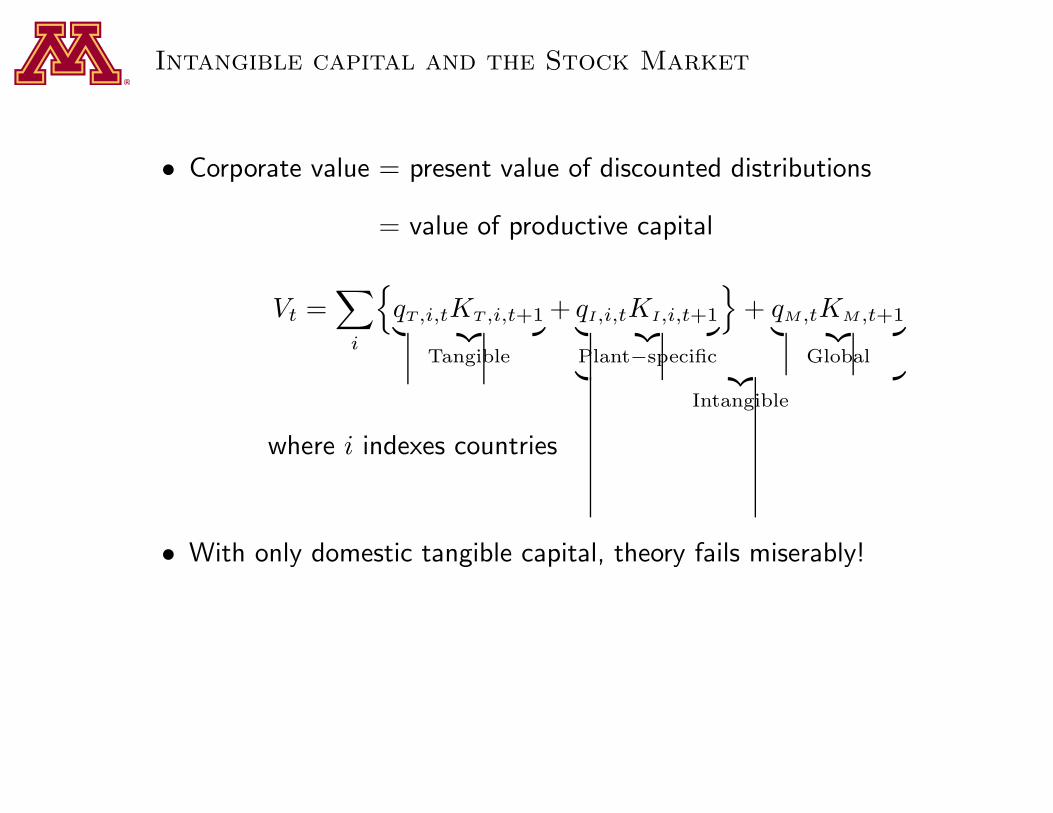
Intangible capital and the Stock Market
• Corporate value = present value of discounted distributions
= value of productive capital
Vt =∑
i
qT ,i,tKT ,i,t+1︸ ︷︷ ︸
Tangible
+ qI,i,tKI,i,t+1︸ ︷︷ ︸
Plant−specific
+ qM,tKM,t+1︸ ︷︷ ︸
Global︸ ︷︷ ︸
Intangible
where i indexes countries
• With only domestic tangible capital, theory fails miserably!

Dramatic Rise in US Values, But KT/GDP≈ 1
Rel
ativ
e to
GD
P
1960 1965 1970 1975 1980 1985 1990 1995 20000
0.5
1
1.5
2
0
0.5
1
1.5
2
Total value
Equity value

Dramatic Rise in Both US and UK
Rel
ativ
e to
GD
P
1960 1965 1970 1975 1980 1985 1990 1995 20000
0.5
1
1.5
2
2.5
0
0.5
1
1.5
2
2.5
United Kingdom
United States

Theory Yields Some Surprising Results
• Stock values should have been high in the 1990s and were.
• Values to GDP should have doubled between the 60s and 90s and did
• PE ratios should have doubled over the same period and did

What Drives the Results?
• Significant changes in prices of capital (q’s)

A Simple Theory
• Preferences:
∑∞t=0 β
tU(ct, ℓt)Nt
• Technologies:
y1,t = f c(k1T,t, k1I,t, ztn1,t) 1=corporate, T,I=tangible,intangible
y2,t = fnc(k2,t, ztn2,t) 2=noncorporate
yt = F (y1,t, y2,t)
Variables:
c = consumption, ℓ = leisure, N = household size
y = output, k = capital, n = labor, z = technology

The U.S. Tax System
• and the Corporation:
max∞∑
t=0
ptp1,ty1,t − wtn1,t − x1T,t − x1I,t
− τ1,t[p1,ty1,t − wtn1,t − δ1Tk1T,t − τ1k,tk1T,t − x1I,t
]
− τ1k,tk1T,t
• and the Household (no capital gains case):
∞∑
t=0
pt(1 + τc,t)ct + V1s,t(s1,t+1−s1,t) + V2s,t(s2,t+1−s2,t) + Vb,tbt+1
≤∞∑
t=0
pt(1− τd,t)d1,ts1,t + d2,ts2,t + bt + (1− τn,t)wtnt + κt

Main Theoretical Result
Vt = (1− τdt) [k1T,t+1 + (1− τ1t)k1I,t+1]
V value of corporate equities
τd tax rate on dividends
k1T tangible corporate capital stock
τ1 tax rate on corporate income
k1I intangible corporate capital stock

Main Theoretical Result
Vt = (1− τdt) [k1T,t+1 + (1− τ1t)k1I,t+1]
• Proposition.
If τdt constant and revenues lump-sum rebated,
then capital-output ratios independent of τd
Proof. τd drops out of intertemporal condition
• Corollary. Periods of high τd have low V /GDP and vice versa

Therefore...
• Stock values should have been high in the 1990s and were.
• Values to GDP should have doubled between the 60s and 90s and did
• Values to GDP should have doubled between the 60s and 90s and did
• PE ratios should have doubled over the same period and did

Taxes–affecting q’s–and Intangibles Important
1960-69 1998-01
Predicted fundamental values
Domestic tangible capital .56 .84
Domestic intangible capital .23 .35
Foreign capital .09 .38
Total relative to GDP .88 1.57
Price-earnings ratio 13.5 27.5
Actual values
Corporate equities .90 1.58
Net corporate debt .04 .03
Total relative to GDP .94 1.60
Price-earnings ratio 14.5 28.1

Recap of Stock Market Study
• Value of US corporations doubled between 1960s and 1990s
• We asked,
Was the stock market overvalued in 1999?
Why did the value double?

Recap of Stock Market Study
• Value of US corporations doubled between 1960s and 1990s
• We asked,
Was the stock market overvalued in 1999?
— by 0.2 GDP (probably not statistically significant)
Why did the value double?
— effective taxes on corporate distributions fell

Recap of Stock Market Study
• Value of US corporations doubled between 1960s and 1990s
• We asked,
Was the stock market overvalued in 1999?
— by 0.2 GDP (probably not statistically significant)
Why did the value double?
— effective taxes on corporate distributions fell
• And, we found that intangible capital is important factor

Went From One Puzzle to the Next...
Our Estimate of Foreign Capital Value
• Since US multinationals do significant FDI,
Computed estimate of value
After the fact, we compared them

Our Estimate of Foreign Capital Value
• Since US multinationals do significant FDI,
Computed estimate of value—not realizing BEA provides one
After the fact, we compared them

Our Estimate of Foreign Capital Value
• Since US multinationals do significant FDI,
Computed estimate of value—not realizing BEA provides one
After the fact, we compared them
Were the BEA and our estimates close?

Our Estimate of Foreign Capital Value
• Since US multinationals do significant FDI,
Computed estimate of value—not realizing BEA provides one
After the fact, we compared them
Were the BEA and our estimates close? No!

Stumbled Upon Another Puzzle
• For US subsidiaries, BEA reports
Small value for capital abroad
Large value for profits from abroad
⇒ Large return to DI of US
• For foreign subsidiaries in US, BEA reports
Small value for capital in US
Really small value for profits
⇒ Small return to DI in US
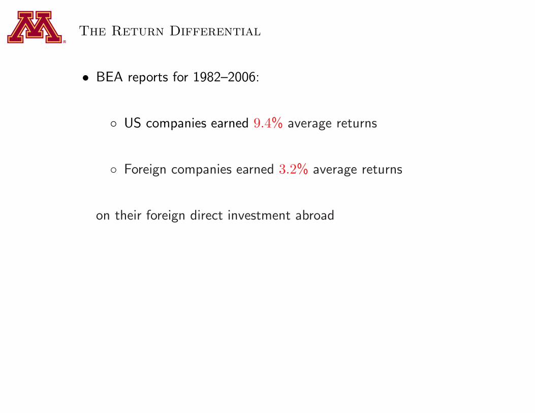
The Return Differential
• BEA reports for 1982–2006:
US companies earned 9.4% average returns
Foreign companies earned 3.2% average returns
on their foreign direct investment abroad

What Could Account for Return Differential?
• Multinationals have large intangible capital stocks
DI profits include intangible rents (+) less expenses (−)
DI stocks don’t include intangible capital
⇒ BEA returns not equal economic returns
• FDI in US is negligible until late 1970s
⇒ Timing of investments different in US & ROW

To Interpret the Data
• Need to consider nature of intangibles
Rival versus nonrival
Expensed at home versus abroad
• Want theory that incorporates these

Extensions to Neoclassical Theory
• Add two types of intangible capital
1. Rival that is plant-specific (KI)
2. Nonrival that is firm-specific (M)
• Add locations since technology capital nonrival (N)
• To otherwise standard multi-country DSGE model

A Useful Example
• US drug company with employees
Bob who develops a new drug in NC
50 drug reps at 50 US locations
2 drug reps at 2 Belgian locations
• Measuring impact of intangibles, need to keep in mind
Some capital is nonrival, some rival
Production opportunities vary with country size
Profits depend on timing of investments and rents
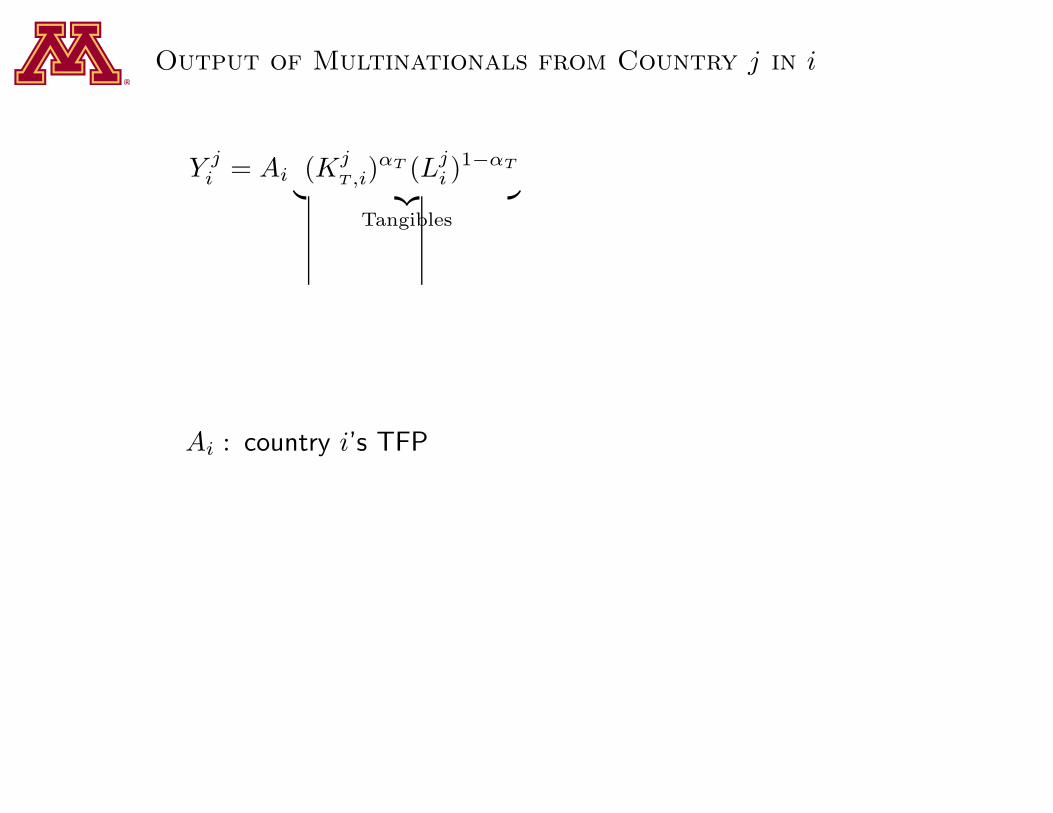
Output of Multinationals from Country j in i
Y ji = Ai (Kj
T ,i)αT (Lj
i )1−αT
︸ ︷︷ ︸
Tangibles
Ai : country i’s TFP

Output of Multinationals from Country j in i
Y ji = Ai (Kj
T ,i)αT (Lj
i )1−αT
︸ ︷︷ ︸
Tangibles
−αI (KjI,i)
αI
︸ ︷︷ ︸
Add KI
Ai : country i’s TFP

Output of Multinationals from Country j in i
Y ji = Ai ((K
jT ,i)
αT (Lji )
1−αT
︸ ︷︷ ︸
Tangibles
−αI (KjI,i)
αI
︸ ︷︷ ︸
Add KI
)1−φ (NiMj)φ
︸ ︷︷ ︸
Add M
Ai : country i’s TFP
Ni : country i’s measure of production locations

Output of Multinationals from Country j in i
Y ji = Ai ((K
jT ,i)
αT (Lji )
1−αT
︸ ︷︷ ︸
Tangibles
−αI (KjI,i)
αI
︸ ︷︷ ︸
Add KI
)1−φ (NiMj)φ
︸ ︷︷ ︸
Add M
(drug reps) (Bob)
Ai : country i’s TFP
Ni : country i’s measure of production locations

Output of Multinationals from Country j in i
Y ji = Ai ((K
jT ,i)
αT (Lji )
1−αT
︸ ︷︷ ︸
Tangibles
−αI (KjI,i)
αI
︸ ︷︷ ︸
Add KI
)1−φσi(NiMj)φ
︸ ︷︷ ︸
Add M
Ai : country i’s TFP
Ni : country i’s measure of production locations
σi : country i’s degree of openness to FDI

Output of Multinationals from Country j in i
Y ji = Ai ((K
jT ,i)
αT (Lji )
1−αT
︸ ︷︷ ︸
Tangibles
−αI (KjI,i)
αI
︸ ︷︷ ︸
Add KI
)1−φσi(NiMj)φ
︸ ︷︷ ︸
Add M
Aji = Y j
i /((KjT ,i)
αT (Lji )
1−αT )
= Aiσi(KjI,i/L
ji )
αI(1−φ)(NiMj)φ
Ai : country i’s TFP
Ni : country i’s measure of production locations
σi : country i’s degree of openness to FDI
Aji : multinational j’s measured TFP in i

Output of Multinationals from Country j in i
Y ji = Ai ((K
jT ,i)
αT (Lji )
1−αT −αI (KjI,i)
αI
︸ ︷︷ ︸
≡Zj
i
)1−φσi(NiMj)φ
︸ ︷︷ ︸
Add M
Aji = Y j
i /((KjT ,i)
αT (Lji )
1−αT )
= Aiσi(KjI,i/L
ji )
αI(1−φ)(NiMj)φ
Next, aggregate over output of all multinationals j

New Aggregate Production Function
Yit = AitNφit(M
it + σ
1φ
it
∑
j 6=iMjt )
φZ1−φit
• Key results:
Output per effective person increasing in size
Greater openness (σit) yields intangible gains
Note: Size ≡ A1
1−(αT +αI )(1−φ)
i Ni

Use theory to Construct BEA Return on FDI
• Think of d=Dell, f=France
rFDI,t = (1− τp,ft)(Y dft −WftL
dft − δTK
dT ,ft −Xd
I,ft
)/Kd
T ,ft
= rt + (1−τp,ft) [φ+ (1−φ)αI]Y dft
KdT ,ft
︸ ︷︷ ︸
intangible rents
−(1−τp,ft)Xd
I,ft
KdT ,ft
︸ ︷︷ ︸
expenses
where rt is actual return on all types of capital

What We Find
• Use model where each investment earns 4.6% on average
• We find average BEA returns on DI, 1982–2006:
of US = 7.1% .... BEA reports 9.4%
in US = 3.1% .... BEA reports 3.2%
⇒ Mismeasurement accounts for over 60% of return gap

Recap of Two Puzzles
• In studying stock market boom, needed estimate of foreign capital
• Our estimates turned out to be much larger than BEA’s
BEA returns are not equal to economic returns
Timing of investments different in US and ROW

Recap of Two Puzzles
• In studying stock market boom, needed estimate of foreign capital
• Our estimates turned out to be much larger than BEA’s
BEA returns are not equal to economic returns
Timing of investments different in US and ROW
• Working on these projects gave us an idea for the 1990s boom

Intangible Capital and the Puzzling 1990s Boom

The Puzzle
1990 1992 1994 1996 1998 2000 200288
90
92
94
96
98
100
102
104
106
US Per Capita Hours
One-Sector Growth Model Per Capita Hours

Connecting the dots...
• Previous work points to issue of mismeasurement
1990s was a tech boom
Yet, TFP was not growing fast
Why? because of large intangible investments in
— Sweat equity
— Corporate R&D

Modeling the Tech Boom
• Two key factors:
Intangible capital that is expensed
Nonneutral technology change w.r.t. its production
• Idea: model tech boom as boom in intangible production

Modeling the Tech Boom
• Two key factors:
Intangible capital that is expensed
Nonneutral technology change w.r.t. its production
• Idea: model tech boom as boom in intangible production
⇒ Increased hours in intangible production

Modeling the Tech Boom
• Two key factors:
Intangible capital that is expensed
Nonneutral technology change w.r.t. its production
• Idea: model tech boom as boom in intangible production
⇒ Increased hours in intangible production
Increased intangible investment

Modeling the Tech Boom
• Two key factors:
Intangible capital that is expensed
Nonneutral technology change w.r.t. its production
• Idea: model tech boom as boom in intangible production
⇒ Increased hours in intangible production
Increased intangible investment
Understated growth in measured productivity

Intuition
• True productivity
yt + qtxIt
hyt + hxt6=
ythyt + hxt
= Measured productivity
whereyt = output of final goods and services
qtxIt = output of intangible production
hyt = hours in production of final G&S
hxt = hours in production of new intangibles
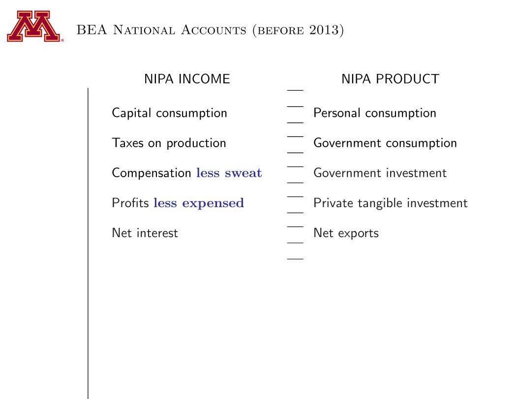
BEA National Accounts (before 2013)
NIPA INCOME NIPA PRODUCT
Capital consumption Personal consumption
Taxes on production Government consumption
Compensation less sweat Government investment
Profits less expensed Private tangible investment
Net interest Net exports

Revised National Accounts
TOTAL INCOME TOTAL PRODUCT
Capital consumption Personal consumption
Taxes on production Government consumption
Compensation less sweat Government investment
Profits less expensed Private tangible investment
Net interest Net exports
Capital gains Intangible investment

Revised National Accounts
TOTAL INCOME TOTAL PRODUCT
Capital consumption Personal consumption
Taxes on production Government consumption
Compensation Government investment
Profits Private tangible investment
Net interest Net exports
Intangible investment

Evidence of the Mechanism
• Macro
Hours boomed, but compensation per hour fell
GDP rose, but corporate profits fell
Capital gains high at end of 1990s
• Micro
Industry R&D boomed
IPO gross proceeds boomed
Average hours boomed selectively

Average Hours Boomed Selectively
Hours Per Noninstitutional Population Aged 16-64
Total The Educated in(1992=100) Select Occupations†
1992 100.0 10.3
2000 106.5 13.3
% Chg. 6.5 30.0
† Managerial, computational, and financial occupations

Theory with Intangibles and Nonneutral Technology
• Household/Business owners solve
maxE
∞∑
t=0
βt[log ct + ψ log(1− ht)]Nt
subject to
ct + xTt + qtxIt = rTtkTt + rItkIt + wtht
−taxest+transferst+nonbusinesst
kT,t+1 = (1− δT )kTt + xTt
kI,t+1 = (1− δI)kIt + xIt
where subscript T/I denotes tangible/intangible
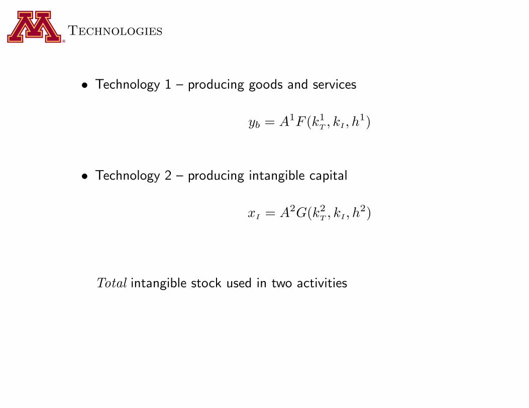
Technologies
• Technology 1 – producing goods and services
yb = A1F (k1T, kI, h
1)
• Technology 2 – producing intangible capital
xI = A2G(k2T, kI, h
2)
Total intangible stock used in two activities

Two Types of Intangible Investment
• Expensed: capital owners finance χ with reduced profits
• Sweat: worker owners finance 1−χ with reduced wages
Choice of χ has tax implications

Hypothesis for the 1990s
• Technological change was nonneutral: A2t/A
1t ↑

Hypothesis for the 1990s
• Technological change was nonneutral: A2t/A
1t ↑
⇒ More hours to intangible sector: h2t/h1t ↑

Hypothesis for the 1990s
• Technological change was nonneutral: A2t/A
1t ↑
⇒ More hours to intangible sector: h2t/h1t ↑
⇒ Measured productivity pNIPA
t falls
pNIPA
t ∝ybt
h1t + h2t

Hypothesis for the 1990s
• Technological change was nonneutral: A2t/A
1t ↑
⇒ More hours to intangible sector: h2t/h1t ↑
⇒ Measured productivity pNIPA
t falls
While true productivity pt rises
pt ∝ybth1t
=ybt + qtxIt
h1t + h2t

The Labor Wedge
• CKM’s labor wedge, 1− τlt:
1− τlt = ψ1 + τct1− τht
·ctybt
·ht
1− ht
= ψ1 + τct1− τht
·ctybt
·h1t
1− ht·hth1t
= 1 +h2th1t
= 1 +qtxIt
ybt
which is rising over the 1990s

Quantitative Predi tions

Identifying TFPs
• Need inputs and outputs of production
Split of hours and tangible capital in 2 activities
Magnitude of intangible investment and capital

Identifying TFPs
• Need inputs and outputs of production
Split of hours and tangible capital in 2 activities
Magnitude of intangible investment and capital
⇐ Determined by factor price equalization

Identifying TFPs
• Need inputs and outputs of production
Split of hours and tangible capital in 2 activities
Magnitude of intangible investment and capital
⇐ Determined by factor price equalization
• Only requires observations on NIPA products and CPS hours

Compute Equilibrium Paths
• Computed both
Perfect foresight paths
Stochastic simulations
Results were insensitive to choice
Next, reconsider the prediction of per capita hours

Equilibrium Per Capita Hours
1990 1992 1994 1996 1998 2000 200296
98
100
102
104
106
US Per Capita Hours
Model with Intangible CapitalPer Capita Hours

Downturn of 20082009

Downturn of 2008–2009
• Many who observed:
GDP and hours fall significantly
Labor productivity rise
• Concluded that this time is different

Downturn of 2008–2009
• Many who observed:
Rising credit spreads
Plummeting asset values
• Concluded financial market disruptions responsible

But, is this time different?
• 2008–2009 is “flip side” of 1990s:
GDP and hours depressed, but booming in ’90s
Labor productivity high, but low in ’90s
• In earlier work, found puzzling if abstract from
Intangible investment that is expensed
Nonneutral technology change w.r.t. its production

Application of Theory to 2000s
• Apply “off-the-shelf” model from 1990s study
Feed in paths for TFPs and tax rates
Abstract from financial and labor market disruptions
• Main findings:
Productivity growth slow-down big part of story
Aggregate observations in conformity with theory

Application of Theory to 2000s
• Apply “off-the-shelf” model from 1990s study
Feed in paths for TFPs and tax rates
Abstract from financial and labor market disruptions
• Main findings:
Productivity growth slow-down big part of story
Aggregate observations in conformity with theory
Is there any empirical evidence?

BEA Comprehensive Revision 2013
• Intellectual property products investment included:
R&D
Artistic originals
Software (first introduced in 1999)
• While much investment still missing, category is large...

BEA Comprehensive Revision 2013
• Private fixed nonresidential investment, 2012
22% Structures
45% Equipment
33% Intellectual property
• Also have data for detailed industrial sectors

Computer & Electronic Products
2007
Inve
stm
ent t
otal
= 1
00
1975 1980 1985 1990 1995 2000 2005 20100
20
40
60
80
100
120
Intellectual propertyEquipmentStructures
Computer & Electronic Products (NAICS 334)

Information
2007
Inve
stm
ent t
otal
= 1
00
1975 1980 1985 1990 1995 2000 2005 20100
20
40
60
80
Intellectual propertyEquipmentStructures
Information (NAICS 51)

Other Microevidence
• SEC requires 10-K reports from public companies
• Have company info on
R&D expenses
Advertising expenses
• Data show simultaneous large declines in 2008–2009

Top 500 Advertisers (COMPUSTAT)
% of Domestic % Decline inStatistic company total 2008–2009
Ad expenses 96.5 -10.8
R&D expenses 46.6 -16.2
PP&E expenses 27.5 -18.2
Employees 50.2 -2.2
Sales 38.6 -3.5

Top 500 R&D Spenders (COMPUSTAT)
% of Domestic % Decline inStatistic company total 2008–2009
Ad expenses 44.7 -19.6
R&D expenses 92.3 -11.9
PP&E expenses 25.9 -21.7
Employees 24.4 -4.4
Sales 34.2 -15.3

Strong I-O Linkages
• Use BEA’s 2007 input-output benchmark
• Find 66% of output has intermediate uses from
Manufacturing (NAICS 31-33)
Information (NAICS 51)
Professional and business services (NAICS 54-56)
• And to sectors that do much less intangible investment

Recap
• Intangible investments are:
Expensed for tax purposes
Only partly measured in GDP
Estimated to be as large as tangibles
Correlated with tangibles
Picked up in typical productivity measures
• And, in our view, worthy of further investigation

Future research needed
• Need full exploration of microevidence for 2008-2009
• Main challenge is using theory to measure the unmeasured

Recap of Lecture II
Not everything that counts can be counted, and
not everything that can be counted counts.
— Albert Einstein

III. Back to methods: Nonlinearities and large state spaces

Lectures at the EUI 1996
• Marimon, R. and A. Scott
Computational Methods for the Study of Dynamic Economies
Oxford University Press, 1999
“Application of weighted residual methods to dynamic economic models”
• Finite element method has proven useful for:
Problems with nonlinearities (kinks, discontinuities)
Problems with large state spaces (exploits sparseness)
Today, will describe method in context of Aiyagari & McGrattan

Aiyagari-McGrattan (1998)
• Study economies with
Large number of infinitely-lived households
Borrowing constraints
Precautionary savings motives
⇒ Savings decision functions have kinks
Distribution of asset holdings have discontinuities

Aiyagari-McGrattan (1998)
• Consumer problem:
maxct,at+1,ℓt
E[
∞∑
t=0
(β(1 + g)η(1−µ))t(cηt ℓ1−ηt )1−µ/(1− µ)|a0, e0
]
s.t. ct + (1 + g)at+1 ≤ (1 + r)at + wet(1− ℓt) + χ
at ≥ 0
ℓt ≤ 1
et : Markov chain
where after-tax rates w, r and transfers χ given

Aiyagari-McGrattan (1998)
• Consumer problem:
maxct,at+1,ℓt
E[
∞∑
t=0
(β(1 + g)η(1−µ))t(cηt ℓ1−ηt )1−µ/(1− µ)|a0, e0
]
s.t. ct + (1 + g)at+1 ≤ (1 + r)at + wet(1− ℓt) + χ
at ≥ 0
ℓt ≤ 1
et : Markov chain
where after-tax rates w, r and transfers χ given
Restrictions on at, et ⇒ kinks, discontinuities

Let’s get rid of constraints
• Modified objective (β = β(1 + g)η(1−µ)):
E
[ ∞∑
t=0
βt
(cηt ℓ
1−ηt )1−µ
1− µ+ζ
3(min(at, 0)
3 +min(1− ℓt, 0)3)
|a0, e0
]
• Solve a sequence of problems with ζ = 1, 10, 100, etc.
• Want: functions c(x, i), ℓ(x, i), α(x, i) = a′ that solve FOCs

Really only need to find α(x, i)
• c(x, i) from budget constraint given α(x, i)
• ℓ(x, i) from intratemporal condition given α(x, i)
Note: in case of ℓ need a robust Newton routine

Boils down to...
• Find α(x, i) to set R(x, i;α) = 0:
R(x, i;α) = η(1 + g)c(ℓ∗(x, i;α))η(1−µ)−1ℓ∗(x, i;α)(1−η)(1−µ)
− β(1 + g)η(1−µ)∑
j
πi,j η(1 + r)c(ℓ∗(α(x, i), j;α))η(1−µ)−1
· ℓ∗(α(x, i), j;α)(1−η)(1−µ) + ζmin(α(x, i), 0)2,
where c∗(x, i;α), ℓ∗(x, i;α) from static FOCs

Applying the Finite Element Method
• Find αh(x, i) to set R(x, i;αh) ≈ 0
• Steps (for Galerkin variant with linear bases):
1. Partition [0, xmax], with subintervals called elements
2. Define αh on [xe, xe+1]:
αh(x, i) = ψieNe(x) + ψi
e+1Ne+1(x)
Ne(x) =xe+1 − x
xe+1 − xe, Ne+1(x) =
x− xexe+1 − xe
3. Find ψie’s to satisfy
F (~ψ) =
∫
R(x, i;αh)Ne(x)dx = 0, i = 1, . . . ,m, e = 1, . . . n.
⇒ Solve mn nonlinear equations in mn unknowns

Practicalities
• It helps to...
Adapt the grid to optimally partition the grid
Compute analytical derivatives dF/dψie to get speed
Exploit sparseness of jacobian matrix

Computing the Invariant Distribution
• Want equilibrium prices r, w
• Need H(x, i) = Pr(xt < x | et = e(i)) which solves:
H(x, i) =
m∑
j=1
πj,iH(α−1(x, j), j)I(x ≥ α(0, j)), I(x > y) = 1 if x > y
• Can again apply FEM to this

Computing the Invariant Distribution
• Want equilibrium prices r, w
• Need H(x, i) = Pr(xt < x | et = e(i)) which solves:
H(x, i) =
m∑
j=1
πj,iH(α−1(x, j), j)I(x ≥ α(0, j)), I(x > y) = 1 if x > y
• Can again apply FEM to this
• How well does it work given the kinks and discontinuities?

Test Cases with Known Solutions
• For test of α(x, i) computation, assume labor inelastic and et = 1
• For test of H(x, i) computation,
Make up a tractible α(x, i) that
Generates known invariant distribution

Testing α(x, i)
• Consumer problem:
maxct,at+1
∞∑
t=0
βtu(ct)
subject to ct + at+1 = (1 + r)at + w
• Solution is piecwise linear and analytically computed

Testing α(x, i)–Grid known
Exact Approximate
0 0.2 0.4 0.6 0.8 1 1.20
0.1
0.2
0.3
0.4
0.5
0.6
0.7
0.8
0.9
1

Testing α(x, i)–Grid known
Exact Approximate
0 0.01 0.02 0.03 0.04 0.05 0.06 0.07-0.005
0
0.005
0.01
0.015
0.02
0.025
0.03
0.035
Zoomed in, Boundary conditions not imposed

Testing α(x, i)–Grid known
Exact Approximate
0 0.01 0.02 0.03 0.04 0.05 0.06 0.070
0.005
0.01
0.015
0.02
0.025
0.03
0.035
Zoomed in, Boundary conditions imposed

Testing α(x, i)–Grid not known
Exact Approximate
0 0.01 0.02 0.03 0.04 0.05 0.06 0.07-0.005
0
0.005
0.01
0.015
0.02
0.025
0.03
0.035
Zoomed in, Boundary conditions not imposed

Testing α(x, i)–Grid not known
Exact Approximate
0 0.01 0.02 0.03 0.04 0.05 0.06 0.07-0.005
0
0.005
0.01
0.015
0.02
0.025
0.03
0.035
Zoomed in, Boundary conditions not imposed, Adapt grid
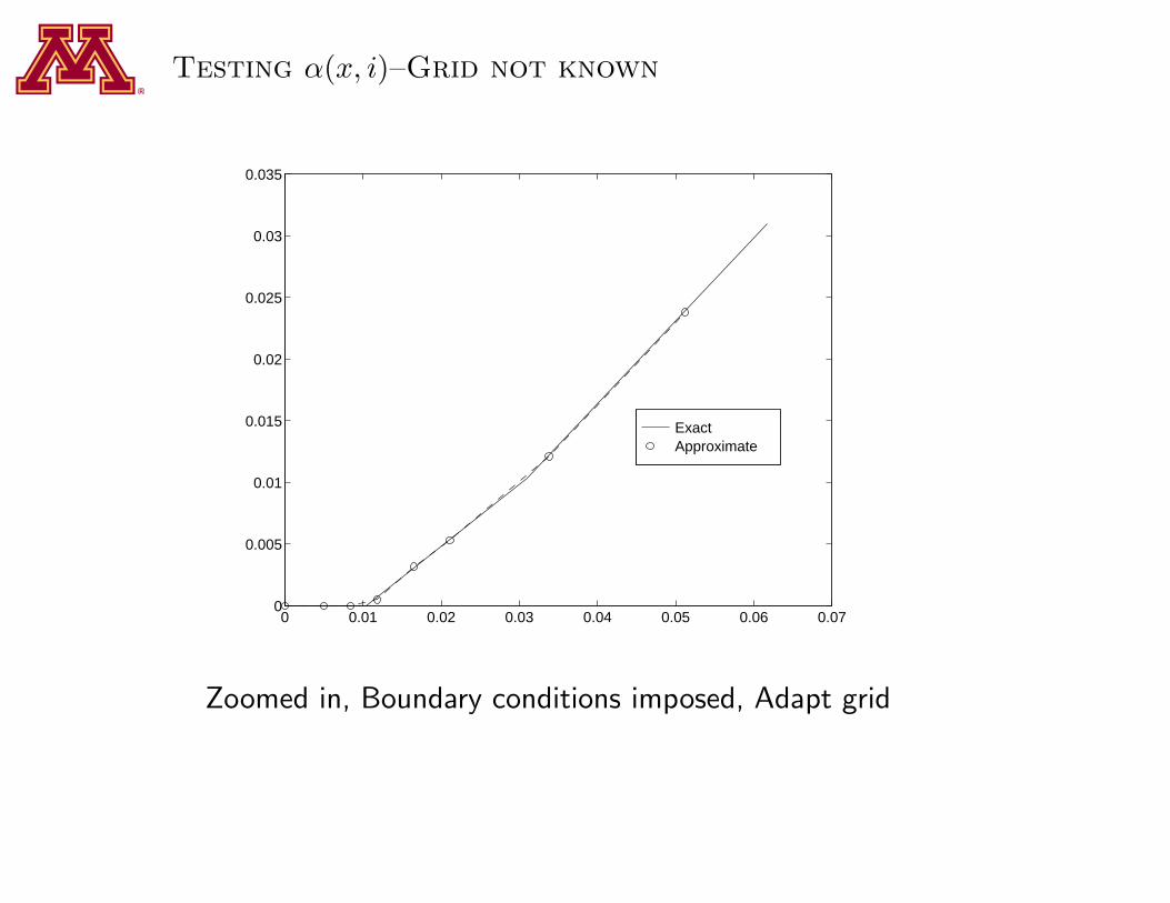
Testing α(x, i)–Grid not known
Exact Approximate
0 0.01 0.02 0.03 0.04 0.05 0.06 0.070
0.005
0.01
0.015
0.02
0.025
0.03
0.035
Zoomed in, Boundary conditions imposed, Adapt grid
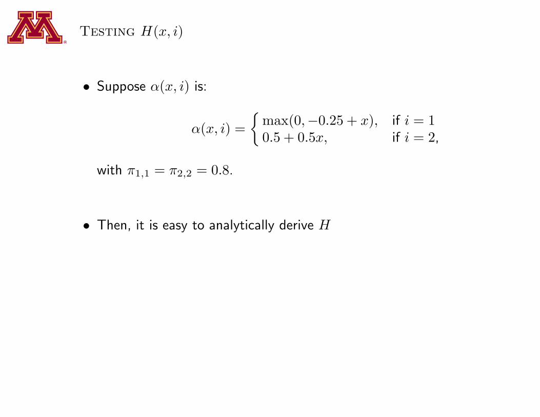
Testing H(x, i)
• Suppose α(x, i) is:
α(x, i) =
max(0,−0.25 + x), if i = 10.5 + 0.5x, if i = 2,
with π1,1 = π2,2 = 0.8.
• Then, it is easy to analytically derive H

Testing H(x, i)—Evenly spaced grid
Exact Approximate
0 0.5 1 1.50.05
0.1
0.15
0.2
0.25
0.3
0.35
0.4
0.45
0.5
0.55
Have n = 13 elements

Testing H(x, i)—Evenly spaced grid
Exact Approximate
0 0.5 1 1.50.05
0.1
0.15
0.2
0.25
0.3
0.35
0.4
0.45
0.5
0.55
Add more elements (n = 25)

Testing H(x, i)—Evenly spaced grid
Exact Approximate
0 0.5 1 1.50.05
0.1
0.15
0.2
0.25
0.3
0.35
0.4
0.45
0.5
0.55
Add more elements (n = 49)

Testing H(x, i)—Evenly spaced grid
Exact Approximate
0 0.5 1 1.50.05
0.1
0.15
0.2
0.25
0.3
0.35
0.4
0.45
0.5
0.55
Add more elements (n = 97)

Testing H(x, i)—Not evenly spaced grid
Exact Approximate
0 0.5 1 1.50.05
0.1
0.15
0.2
0.25
0.3
0.35
0.4
0.45
0.5
0.55
Adapted grid (n = 73)

Future work needed
• Want to solve problems with time-varying distributions Ht

Parallel processing
• Big change since EUI Lectures in 1996: parallel processing
Most problems can be parallelized
OpenMPI simple to use with few changes to existing codes

Recap of Lecture III
• Since 1996, I have
Applied FEM to many interesting problems
Learned to parallelize most of my codes
• But, there is still much to learn!