elements of map-scale structure - ardiansyah kusuma … · chapter 1 elements of map-scale...

Chapter 1

Elements of Map-Scale Structure

1.1Introduction

The primary objective of structural map making and map interpretation is to develop aninternally consistent three-dimensional picture of the structure that agrees with all thedata. This can be difficult or ambiguous because the complete structure is usuallyundersampled. Thus an interpretation of the complete geometry will probably require asignificant number of inferences, as, for example, in the interpolation of a folded surfacebetween the observation points. Constraints on the interpretation are both topologicaland mechanical. The basic elements of map-scale structure are the geometries of foldsand faults, the shapes and thicknesses of units, and the contact types. This chapter pro-vides a short review of the basic elements of the structural and stratigraphic geometriesthat will be interpreted in later chapters, reviews some of the primary mechanical factorsthat control the geometry of map-scale folds and faults, and examines the typical sourcesof data for structural interpretation and their inherent errors.

1.2Representation of a Structure in Three Dimensions

A structure is part of a three-dimensional solid volume that probably contains numer-ous beds and perhaps faults and intrusions (Fig. 1.1). An interpreter strives to develop

Fig. 1.1. 3-D oblique view of a portion of the Black Warrior Basin, Alabama (data from Groshong et al. 2003b),viewed to the NW. Thin vertical lines are wells, semi-transparent surfaces outlined in black are faults

2 Chapter 1 · Elements of Map-Scale Structure

Fig. 1.2. Structure contours. a Lines of equal elevation on the surface of a map unit. b Lines of equalelevation projected onto a horizontal surface to make a structure contour map

Fig. 1.3.Structure contour map of thefaulted upper horizon fromFig. 1.1. Contours are at 50 ftintervals, with negative eleva-tions being below sea level.Faults are indicated by gapswhere the horizon is missing

a mental and physical picture of the structure in three dimensions. The best interpre-tations utilize the constraints provided by all the data in three dimensions. The mostcomplete interpretation would be as a three-dimensional solid, an approach possiblewith 3-D computer graphics programs. Two-dimensional representations of structuresby means of maps and cross sections remain major interpretation and presentationtools. When the geometry of the structure is represented in two dimensions on a mapor cross section, it must be remembered that the structure of an individual horizon ora single cross section must be compatible with those around it. This book presentsmethods for extracting the most three-dimensional interpretive information out oflocal observations and for using this information to build a three-dimensional inter-pretation of the whole structure.

3

1.2.1Structure Contour Map

A structure contour is the trace of a horizontal line on a surface (e.g., on a formationtop or a fault). A structure contour map represents a topographic map of the surfaceof a geological horizon (Figs. 1.2, 1.3). The dip direction of the surface is perpendicu-lar to the contour lines and the dip amount is proportional to the spacing between thecontours. Structure contours provide an effective method for representing the three-dimensional form of a surface in two dimensions. Structure contours on a faultedhorizon (Fig. 1.3) are truncated at the fault.

1.2.2Triangulated Irregular Network

A triangulated irregular network (TIN; Fig. 1.4) is an array of points joined by straightlines that define a surface. In a TIN network, the nearest-neighbor points are connectedto form triangles that form the surface (Banks 1991; Jones and Nelson 1992). If thetriangles in the network are shaded, the three-dimensional character of the surfacecan be illustrated. This is an effective method for the rendering of surfaces by com-puter. The TIN can be contoured to make a structure contour map.

1.2.3Cross Section

Even though a structure contour map or TIN represents the geometry of a surface inthree dimensions, it is only two-dimensional because it has no thickness. To completelyrepresent a structure in three dimensions, the relationship between different horizonsmust be illustrated. A cross section of the geometry that would be seen on the face ofa slice through the volume is the simplest representation of the relationship between

Fig. 1.4. Triangulated irregular network (TIN) of points used to form the upper map horizon in Figs. 1.1 and1.3. 3-D perspective view to the NW, 3× vertical exaggeration. Vertical scale in ft, horizontal scale in meters

1.2 · Representation of a Structure in Three Dimensions


horizons. In this book cross sections will be assumed to be vertical unless it is statedotherwise. A cross section through multiple surfaces illustrates their individual geom-etries and defines the relationships between the surfaces (Fig. 1.5). The geometry ofeach surface provides constraints on the geometry of the adjacent surfaces. The rela-tionships between surfaces forms the foundation for many of the techniques of struc-tural interpretation that will be discussed.

1.3Map Units and Contact Types

The primary concern of this book is the mapping and map interpretation of geologiccontacts and geologic units. A contact is the surface where two different kinds of rockscome together. A unit is a closed volume between two or more contacts. The geometry ofa structure is represented by the shape of the contacts between adjacent units. Dips orlayering within a unit, such as in a crossbedded sandstone, are not necessarily parallel tothe contacts between map units. Geological maps are made for a variety of purposes andthe purpose typically dictates the nature of the map units. It is important to consider thenature of the units and the contact types in order to distinguish between geometriesproduced by deposition and those produced by deformation. Units may be either rightside up or overturned. A stratigraphic horizon is said to face in the direction toward whichthe beds get younger. If possible, the contacts to be used for structural interpretation shouldbe parallel and have a known paleogeographic shape. This will allow the use of a numberof powerful rules in the construction and validation of map surfaces, in the constructionof cross sections, and should result in geometries that can be restored to their originalshapes as part of the structural validation process. Contacts that were originally horizon-tal are preferred. Even if a restoration is not actually done, the concept that the map unitswere originally horizontal is implicit in many structural interpretations.

Fig. 1.5. East-west cross section across the structure in Fig. 1.1 produced by taking a vertical slice throughthe 3-D model. Line of section shown on Fig. 1.3

5

1.3.1Depositional Contacts

A depositional contact is produced by the accumulation of material adjacent to thecontact (after Bates and Jackson 1987). Sediments, igneous or sedimentary extrusions,and air-fall igneous rocks have a depositional lower contact which is parallel to thepre-existing surface. The upper surface of such units is usually, but not always, close tohorizontal. A conformable contact is one in which the strata are in unbroken sequenceand in which the layers are formed one above the other in parallel order, representingthe uninterrupted deposition of the same general type of material, e.g., sedimentary orvolcanic (after Bates and Jackson 1987).

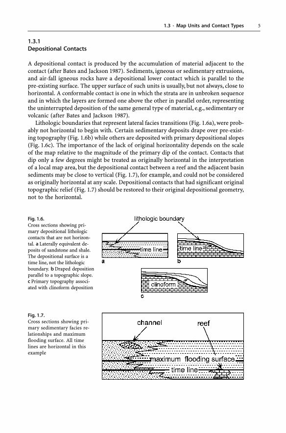
Lithologic boundaries that represent lateral facies transitions (Fig. 1.6a), were prob-ably not horizontal to begin with. Certain sedimentary deposits drape over pre-exist-ing topography (Fig. 1.6b) while others are deposited with primary depositional slopes(Fig. 1.6c). The importance of the lack of original horizontality depends on the scaleof the map relative to the magnitude of the primary dip of the contact. Contacts thatdip only a few degrees might be treated as originally horizontal in the interpretationof a local map area, but the depositional contact between a reef and the adjacent basinsediments may be close to vertical (Fig. 1.7), for example, and could not be consideredas originally horizontal at any scale. Depositional contacts that had significant originaltopographic relief (Fig. 1.7) should be restored to their original depositional geometry,not to the horizontal.

Fig. 1.6.Cross sections showing pri-mary depositional lithologiccontacts that are not horizon-tal. a Laterally equivalent de-posits of sandstone and shale.The depositional surface is atime line, not the lithologicboundary. b Draped depositionparallel to a topographic slope.c Primary topography associ-ated with clinoform deposition

Fig. 1.7.Cross sections showing pri-mary sedimentary facies re-lationships and maximumflooding surface. All timelines are horizontal in thisexample

1.3 · Map Units and Contact Types


1.3.2Unconformities

An unconformity is a surface of erosion or nondeposition that separates younger stratafrom older strata. An angular unconformity (Fig. 1.8a) is an unconformity betweentwo groups of rocks whose bedding planes are not parallel. An angular unconformitywith a low angle of discordance is likely to appear conformable at a local scale. Distin-guishing between conformable contacts and low-angle unconformities is difficult butcan be extremely important to the correct interpretation of a map. A progressive or but-tress unconformity (Fig. 1.8b; Bates and Jackson 1987) is a surface on which onlappingstrata abut against a steep topographic scarp of regional extent. A disconformity (Fig. 1.8c)is an unconformity in which the bedding planes above and below the break are essen-tially parallel, indicating a significant interruption in the orderly sequence of sedi-mentary rocks, generally by an interval of erosion (or sometimes of nondeposition),and usually marked by a visible and irregular or uneven erosion surface of appreciablerelief. A nonconformity (Fig. 1.8d) is an unconformity developed between sedimen-tary rocks and older plutonic or massive metamorphic rocks that had been exposed toerosion before being covered by the overlying sediment.

1.3.3Time-Equivalent Boundaries

The best map-unit boundaries for regional structural and stratigraphic interpretationare time-equivalent across the map area. Time-equivalent boundaries are normallyestablished using fossils or radiometric age dates and may cross lithologic boundaries.Volcanic ash fall deposits, which become bentonites after diagenesis, are excellent timemarkers. Because an ash fall drapes the topography and is relatively independent ofthe depositional environment, it can be used for regional correlation and to determinethe depositional topography (Asquith 1970). It can be difficult to establish time-equiva-lent map horizons because of the absence or inadequate resolution of the paleonto-logic or radiometric data, lithologic and paleontologic heterogeneity in the deposi-tional environment, and because of the occurrence of time-equivalent nondepositionor erosion in adjacent areas. Time-equivalent map-unit boundaries may be based oncertain aspects of the physical stratigraphy. A sequence is a conformable succession of

Fig. 1.8.Unconformity types. The un-conformity (heavy line) is thecontact between the older, un-derlying shaded units and theyounger, overlying unshadedunits. a Angular unconformity.b Buttress or onlap unconfor-mity. c Disconformity. d Non-conformity. The patterned unitmay be plutonic or metamor-phic rock

7

genetically related strata bounded by unconformities and their correlative conformi-ties (Mitchum 1977; Van Wagoner et al. 1988). A parasequence is a subunit within asequence that is bounded by marine flooding surfaces (Van Wagoner et al. 1988) andthe approximate time equivalence along flooding surfaces makes them suitable forstructural mapping. A maximum flooding surface (Fig. 1.7; Galloway 1989) can be thebest for regional correlation because the deepest-water deposits can be correlated acrosslithologic boundaries. At the time of maximum flooding, the sediment input is at aminimum and the associated sedimentary deposits are typically condensed sections,seen as radioactive shales or thin, very fossiliferous carbonates.

1.3.4Welds

A weld joins strata originally separated by a depleted or withdrawn unit (after Jackson1995). Welds are best known where a salt bed has been depleted by substratal dissolu-tion or by flow (Fig. 1.9). If the depleted unit was deposited as part of a stratigraphicallyconformable sequence, the welded contact will resemble a disconformity. If the de-pleted unit was originally an intrusion, like a salt sill, the welded contact will return toits original stratigraphic configuration. A welded contact may be recognized fromremnants of the missing unit along the contact. Lateral displacement may occur acrossthe weld before or during the depletion of the missing unit (Fig. 1.9b). Welded con-tacts may crosscut bedding in the country rock if the depleted unit was originally cross-cutting, as, for example, salt diapir that is later depleted.

1.3.5Intrusive Contacts and Veins

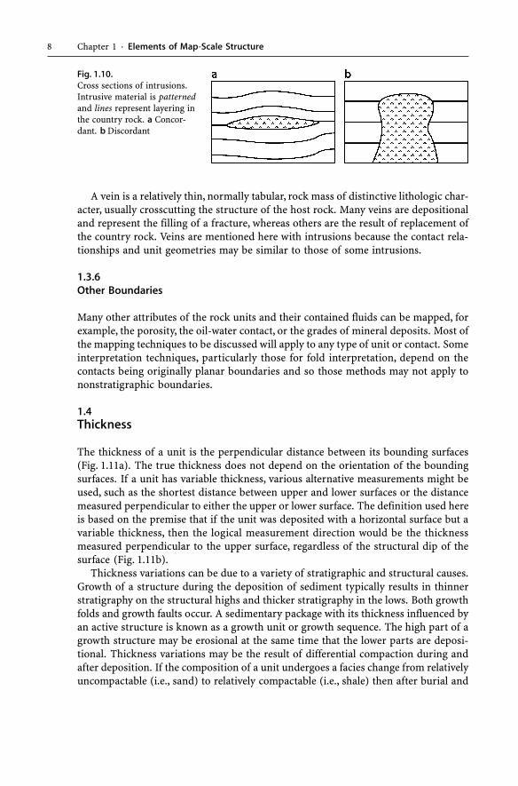
An intrusion is a rock, magma, or sediment mass that has been emplaced into anotherdistinct unit. Intrusions (Fig. 1.10) may form concordant contacts that are parallel tothe layering in the country rock, or discordant contacts that crosscut the layering inthe country rock. A single intrusion may have contacts that are locally concordant anddiscordant.

Fig. 1.9. Cross sections illustrating the formation of a welded contact. Solid dots are fixed materialpoints above and below the unit which will be depleted. a Sequence prior to depletion. b Sequenceafter depletion: solid dots represent the final positions of original points in a hangingwall withoutlateral displacement; open circles represent final positions of original points in a hangingwall withlateral displacement

1.3 · Map Units and Contact Types


A vein is a relatively thin, normally tabular, rock mass of distinctive lithologic char-acter, usually crosscutting the structure of the host rock. Many veins are depositionaland represent the filling of a fracture, whereas others are the result of replacement ofthe country rock. Veins are mentioned here with intrusions because the contact rela-tionships and unit geometries may be similar to those of some intrusions.

1.3.6Other Boundaries

Many other attributes of the rock units and their contained fluids can be mapped, forexample, the porosity, the oil-water contact, or the grades of mineral deposits. Most ofthe mapping techniques to be discussed will apply to any type of unit or contact. Someinterpretation techniques, particularly those for fold interpretation, depend on thecontacts being originally planar boundaries and so those methods may not apply tononstratigraphic boundaries.

1.4Thickness

The thickness of a unit is the perpendicular distance between its bounding surfaces(Fig. 1.11a). The true thickness does not depend on the orientation of the boundingsurfaces. If a unit has variable thickness, various alternative measurements might beused, such as the shortest distance between upper and lower surfaces or the distancemeasured perpendicular to either the upper or lower surface. The definition used hereis based on the premise that if the unit was deposited with a horizontal surface but avariable thickness, then the logical measurement direction would be the thicknessmeasured perpendicular to the upper surface, regardless of the structural dip of thesurface (Fig. 1.11b).

Thickness variations can be due to a variety of stratigraphic and structural causes.Growth of a structure during the deposition of sediment typically results in thinnerstratigraphy on the structural highs and thicker stratigraphy in the lows. Both growthfolds and growth faults occur. A sedimentary package with its thickness influenced byan active structure is known as a growth unit or growth sequence. The high part of agrowth structure may be erosional at the same time that the lower parts are deposi-tional. Thickness variations may be the result of differential compaction during andafter deposition. If the composition of a unit undergoes a facies change from relativelyuncompactable (i.e., sand) to relatively compactable (i.e., shale) then after burial and

Fig. 1.10.Cross sections of intrusions.Intrusive material is patternedand lines represent layering inthe country rock. a Concor-dant. b Discordant

9

compaction the unit thickness will vary as a function of lithology. Deformation-re-lated thickness changes are usually accompanied by folding, faulting, or both withinthe unit being mapped. Deformation-related thickness changes are likely to correlateto position within a structure or to structural dip.

1.5Folds

A fold is a bend due to deformation of the original shape of a surface. An antiform isconvex upward; an anticline is convex upward with older beds in the center. A synformis concave upward; a syncline is concave upward with younger beds in the center.Original curves in a surface, for example grooves or primary thickness changes, arenot considered here to be anticlines or synclines.

1.5.1Styles

Folds may be characterized by domains of uniform dip, by a uniform variation of thedip around a single center of curvature, or may combine regions of both styles. Re-gions of uniform dip (Fig. 1.12a) are called dip domains (Groshong and Usdansky 1988).Dip domains are separated from one another by axial surfaces or faults. Dip domainshave also been referred to as kink bands, but the term kink band has mechanical

Fig. 1.11. Thickness (t). a Unit of constant thickness. b Unit of variable thickness

Fig. 1.12. Regions of uniform dip properties. a Dip domains. b Concentric domains separated by a pla-nar dip domain (shaded)

1.5 · Folds


implications that are not necessarily appropriate for every structure. An axial surface(Fig. 1.12a) is a surface that connects fold hinge lines, where a hinge line is a line ofmaximum curvature on the surface of a bed (Dennis 1967). A hinge (Fig. 1.12a) is theintersection of a hinge line with the cross section. A circular domain (Fig. 1.12b) isdefined here as a region in which beds approximate a portion of a circular arc. Ifmultiple surfaces in a circular domain have the same center of curvature, the fold isconcentric. Dips in a concentric domain are everywhere perpendicular to a radiusthrough the center of curvature. The center of curvature is determined as the intersec-tion point of lines drawn perpendicular to the dips (Busk 1929; Reches et al. 1981). Acircular curvature domain does not possess a line of maximum curvature and thusdoes not strictly have an axial surface. Dips within a domain may vary from the aver-age values. If the dips are measured by a hand-held clinometer, variations of a fewdegrees are to be expected due to the natural variation of bedding surfaces and theimprecision of the measurements.

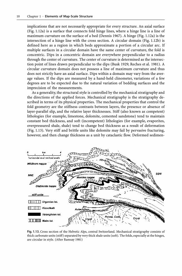
As a generality, the structural style is controlled by the mechanical stratigraphy andthe directions of the applied forces. Mechanical stratigraphy is the stratigraphy de-scribed in terms of its physical properties. The mechanical properties that control thefold geometry are the stiffness contrasts between layers, the presence or absence oflayer-parallel slip, and the relative layer thicknesses. Stiff (also known as competent)lithologies (for example, limestone, dolomite, cemented sandstone) tend to maintainconstant bed thickness, and soft (incompetent) lithologies (for example, evaporites,overpressured shale, shale) tend to change bed thickness as a result of deformation(Fig. 1.13). Very stiff and brittle units like dolomite may fail by pervasive fracturing,however, and then change thickness as a unit by cataclastic flow. Deformed sedimen-

Fig. 1.13. Cross section of the Helvetic Alps, central Switzerland. Mechanical stratigraphy consists ofthick carbonate units (stiff) separated by very thick shale units (soft). The folds, especially at the hinges,are circular in style. (After Ramsay 1981)

11

tary rocks tend to maintain relatively constant bed thickness, although the thicknesschanges that do occur can be very important. If large thickness changes are observedin deformed sedimentary rocks other than evaporites or overpressured shale, primarystratigraphic variations should be considered as a strong possibility.

In cross section, folds may be harmonic, with all the layers nearly parallel to oneanother (Fig. 1.14), or disharmonic, with significant changes in the geometry betweendifferent units in the plane of the section (Figs. 1.13, 1.15). The fold geometry is con-trolled by the thickest and stiffest layers (or multilayers) called the dominant members(Currie et al. 1962). A stratigraphic interval characterized by a dominant (geometry-controlling) member between two boundary zones is a structural-lithic unit (Fig. 1.15;

Fig. 1.14.Dip-domain style folds in anexperimental model havinga closely spaced multilayerstratigraphy. The black andwhite layers are plasticeneand are separated by greaseto facilitate layer-parallel slip.The black layers are slightlystiffer than the white layers.(After Ghosh 1968)

Fig. 1.15. Structural-lithic units. (After Currie et al. 1962)

1.5 · Folds


Currie et al. 1962). A short-wavelength structural lithic unit may form inside the bound-ary of a larger-wavelength unit and be folded by it, in which case the longer-wave-length unit is termed the dominant structural-lithic unit and the shorter-wavelengthunit is a conforming structural-lithic unit (Currie et al. 1962).

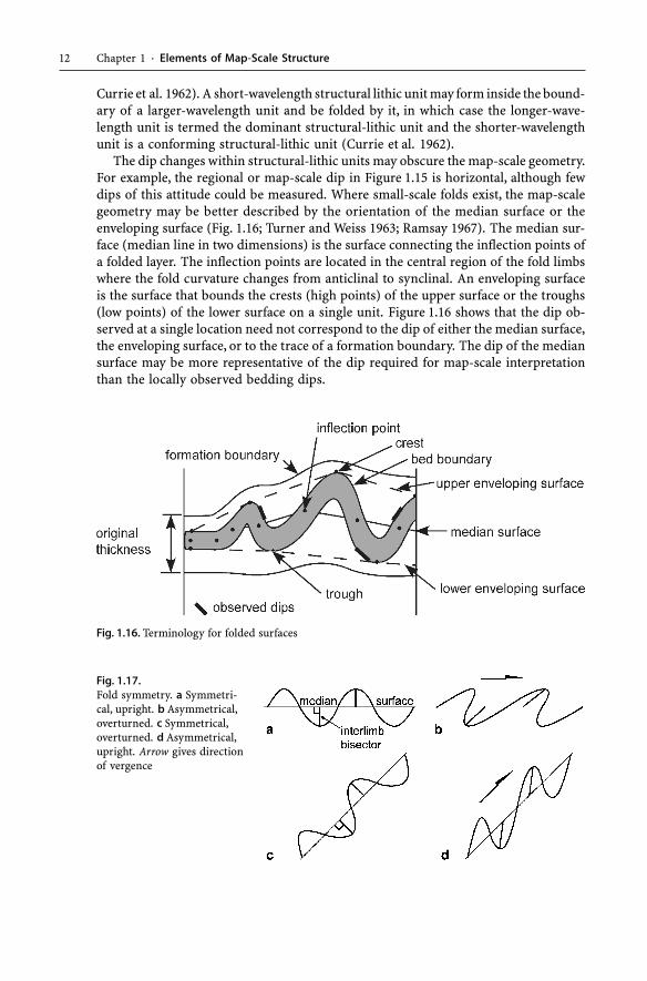
The dip changes within structural-lithic units may obscure the map-scale geometry.For example, the regional or map-scale dip in Figure 1.15 is horizontal, although fewdips of this attitude could be measured. Where small-scale folds exist, the map-scalegeometry may be better described by the orientation of the median surface or theenveloping surface (Fig. 1.16; Turner and Weiss 1963; Ramsay 1967). The median sur-face (median line in two dimensions) is the surface connecting the inflection points ofa folded layer. The inflection points are located in the central region of the fold limbswhere the fold curvature changes from anticlinal to synclinal. An enveloping surfaceis the surface that bounds the crests (high points) of the upper surface or the troughs(low points) of the lower surface on a single unit. Figure 1.16 shows that the dip ob-served at a single location need not correspond to the dip of either the median surface,the enveloping surface, or to the trace of a formation boundary. The dip of the mediansurface may be more representative of the dip required for map-scale interpretationthan the locally observed bedding dips.

Fig. 1.16. Terminology for folded surfaces

Fig. 1.17.Fold symmetry. a Symmetri-cal, upright. b Asymmetrical,overturned. c Symmetrical,overturned. d Asymmetrical,upright. Arrow gives directionof vergence

13

The symmetry of a fold is determined by the angle between the plane bisecting theinterlimb angle and the median surface (Fig. 1.17a; Ramsay 1967). The angle is closeto 90° in a symmetrical fold (Fig. 1.17a,c) and noticeably different from 90° in an asym-metrical fold (Fig. 1.17b,d). An essential property of an asymmetrical fold is that thelimbs are unequal in length. Fold asymmetry is not related to the relative dips of thelimbs. The folds in Fig. 1.17b,c have overturned steep limbs and right-way-up gentlelimbs, but only the folds in Fig. 1.17b are asymmetric. This is a point of possible con-fusion, because in casual usage a fold with unequal limb dips (Fig. 1.17b,c) may bereferred to as being asymmetrical. Folds may occur as regular periodic waveforms asshown (Fig. 1.17) or may be non-periodic with wavelengths that change along themedian surface.

The vergence of an asymmetrical fold is the rotation direction that would rotate theaxial surface of an antiform from an original position perpendicular to the mediansurface to its observed position at a lower angle to the median surface. The vergenceof the folds in Fig. 1.17b,d is to the right.

1.5.2Three-Dimensional Geometry

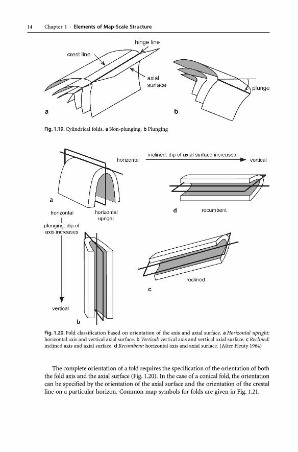
A cylindrical fold is defined by the locus of points generated by a straight line,called the fold axis, that is moved parallel to itself in space (Fig. 1.18a). In otherwords, a cylindrical fold has the shape of a portion of a cylinder. In a cylindricalfold every straight line on the folded surface is parallel to the axis. The geometryof a cylindrical fold persists unchanged along the axis as long as the axis re-mains straight. A conical fold is generated by a straight line rotated through a fixedpoint called the vertex (Fig. 1.18b). The cone axis is not parallel to any line on thecone itself. A conical fold changes geometry and terminates along the trend of thecone axis.

The crest line is the trace of the line which joins the highest points on successivecross sections through a folded surface (Figs. 1.18, 1.19a; Dennis 1967). A trough lineis the trace of the lowest elevation on cross sections through a horizon. The plunge ofa cylindrical fold is parallel to the orientation of its axis or a hinge line (Fig. 1.19b). Themost useful measure of the plunge of a conical fold is the orientation of its crest lineor trough line (Bengtson 1980).

Fig. 1.18. Three-dimensional fold types. a Cylindrical. All straight lines on the cylinder surface are par-allel to the fold axis and to the crestal line. b Conical. V vertex of the cone. Straight lines on the conesurface are not parallel to the cone axis

1.5 · Folds


The complete orientation of a fold requires the specification of the orientation of boththe fold axis and the axial surface (Fig. 1.20). In the case of a conical fold, the orientationcan be specified by the orientation of the axial surface and the orientation of the crestalline on a particular horizon. Common map symbols for folds are given in Fig. 1.21.

Fig. 1.19. Cylindrical folds. a Non-plunging. b Plunging

Fig. 1.20. Fold classification based on orientation of the axis and axial surface. a Horizontal upright:horizontal axis and vertical axial surface. b Vertical: vertical axis and vertical axial surface. c Reclined:inclined axis and axial surface. d Recumbent: horizontal axis and axial surface. (After Fleuty 1964)

15

1.5.3Mechanical Origins

The fundamental mechanical types of folding are based on the direction of the causativeforces relative to layering (Ramberg 1963; Gzovsky et al. 1973; Groshong 1975), namelylongitudinal contraction, transverse contraction, and longitudinal extension (Fig. 1.22).If the stratigraphy is without mechanical contrasts, forces parallel to layering produceeither uniform shortening and thickening or uniform extension and thinning. If someshape irregularity is pre-existing, then it is amplified by layer-parallel shortening togive a passive fold. If the stratigraphy has significant mechanical contrasts, then amechanical instability can occur that leads to buckle folding in contraction and pinch-and-swell structure (boudinage) in extension. If the forces are not equal vertically, thena forced fold is produced, regardless of the mechanical stratigraphy. Longitudinalcontraction, transverse contraction, and longitudinal extension are end-member bound-ary conditions; they may be combined to produce folds with combined properties.

Buckle folds normally form with the fold axes perpendicular to the maximum prin-cipal compressive stress, σ1. The folds are long and relatively unchanging in geometryparallel to the fold axis but highly variable in cross section. Buckle folds are character-ized by the presence of a regular wavelength that is proportional to the thickness of thestiff unit(s). A single-layer buckle fold consists of a stiff layer in a surrounding confin-ing medium. The dip variations associated with a given stiff layer die out into theregional dip within the softer units at a distance of about one-half arc length awayfrom the layer (Fig. 1.15). In the author’s experience, buckle folds in sedimentary rockstypically have arc-length to thickness ratios of 5 to 30, with common values in the rangeof 6 to 10.

As buckled stiff layers become more closely spaced, the wavelengths begin to inter-fere (Fig. 1.23) resulting in disharmonic folds. Once the layers are sufficiently closelyspaced, they fold together as a multilayer unit. A multilayer unit has a much lowerbuckling stress and an appreciably shorter wavelength than a single layer of samethickness (Currie et al. 1962). Stiff units, either single layers or multilayers, tend to

Fig. 1.21. Common map symbols for folds. Fold trend is indicated by the long line, plunge by the arrow-head, with amount of plunge given. The fold trend may be the axial trace, crest or trough line or a hingeline. a, b Anticline. c Overturned anticline; both limbs dip away from the core. d, e Syncline. f Overturnedsyncline; both limbs dip toward the core. g Minor folds showing trend and plunge of axis. h Plungingmonocline with only one dipping limb

1.5 · Folds


produce circular to sinusoidal folds if enclosed in a sufficient thickness of softer ma-terial (Fig. 1.13). Stratigraphic sections made up of relatively thin-bedded multilayerunits result in folds that tend to have planar dip-domain styles (Fig. 1.14).

The strain distribution in the stiff layer of a buckle fold (Fig. 1.24a) is approximatelylayer-parallel shortening throughout most of the fold. The neutral surface separatesregions of layer-parallel extension from regions of layer-parallel contraction. Only ina pure bend (Fig. 1.24b) are the areas of extension and contraction about equal and theneutral surface in the middle of the layer. The strain in thick soft layers between stiff

Fig. 1.23. Transition from single layer folding to multilayer folding as space between stiff layers de-creases. The stiff layers are shaded

Fig. 1.24.Strain distribution shown bystrain ellipses in folded stifflayers. The trace of the neu-tral surface of no strain isdashed. a Buckle fold. b Purebend (Drucker 1967)

Fig. 1.22. End-member displacement boundary conditions showing responses related to the mechani-cal stratigraphy. Shaded beds are stiff lithologies, unshaded beds are soft lithologies

17

layers is shortening approximately perpendicular to the axial surface. The strain inthin soft layers between stiff layers may be close to layer-parallel shear strain. The purebending strain distribution is usually more closely approached in transverse contrac-tion folds, for example above a salt dome, than in buckle folds.

Cleavage planes and tectonic stylolites in a fold can indicate the mechanical originof the fold because they form approximately perpendicular to the maximum shorten-ing direction by processes that range from grain rotation to pressure solution (Groshong1988). Cleavage in a buckle fold is typically at a high angle to bedding (Fig. 1.25), beingmore nearly perpendicular to bedding in stiff units and more nearly parallel to the axialsurface in soft units. Cleavage that is approximately perpendicular to bedding producesa cleavage fan across the fold. The line of the cleavage-bedding intersection is approxi-mately or exactly parallel to the fold axis and can be used to help determine the axis.

Folds produced by an unequal distribution of forces in transverse contraction(Fig. 1.22) are termed forced folds (Stearns 1978). Forced folds tend to be round toblocky or irregular in map view. The major control on the form of the fold is the rhe-ology of the forcing member (Fig. 1.26). A stiff and brittle forcing member (i.e., crys-talline basement) leads to narrow fault boundaries at the base of the structure andstrain that is highly localized in the zone above the basement fault. A soft unit betweena stiff forcing member and the cover sequence will cause the deformation to be dishar-monic. A soft forcing member (like salt) typically produces round to elliptical struc-tures with deformation widely distributed across the uplift.

Little strain need occur in the uplifted or downdropped blocks associated with astiff forcing member. Nearly all the strain is localized in the fault zone between the

Fig. 1.25.Cleavage pattern in a bucklefold. The gently dipping sur-faces are bedding and thesteeply dipping surfaces rep-resent cleavage or stylolites.Arrows show directions ofthe boundary displacements

Fig. 1.26.Effect of mechanical stratigra-phy on drape folds. The lowestunit is the forcing member

1.5 · Folds


blocks or in the steep limb of the drape fold over the fault zone. A soft forcing member(i.e., salt) will distribute the curvature and strain widely over the uplifted region(Fig. 1.27a). Because cleavage and stylolites form perpendicular to the shortening di-rection, in folds produced by displacements at a high angle to bedding, the expectedcleavage and stylolite direction is parallel to bedding (Fig. 1.27b). In highly deformedrocks, cleavage parallel to bedding might be the result of deformation caused by a largeamount of layer-parallel slip or by isoclinal refolding of an earlier axial-plane cleavage.

Extension fractures and veins may form due to the bending stresses in the outer arcof a fold (Fig. 1.28). Such features should become narrower and die out toward theneutral surface. The fracture plane is expected to be approximately parallel to the axisof the fold and the fracture-bedding line of intersection should be parallel to the foldaxis. Bending fractures might occur in any type of fold.

1.6Faults

A fault (Fig. 1.29) is a surface or narrow zone across which there has been relative dis-placement of the two sides parallel to the zone (after Bates and Jackson 1987). Theterm displacement is the general term for the relative movement of the two sides of thefault, measured in any chosen direction. A shear zone is a general term for a relativelynarrow zone with subparallel boundaries in which shear strain is concentrated (Mitraand Marshak 1988). As the terms are usually applied, a bed, foliation trend, or othermarker horizon maintains continuity across a shear zone but is broken and displaced

Fig. 1.27. Strain and cleavage patterns in transverse contraction folds produced by differential verticaldisplacement. a Strain distribution above a model salt dome (after Dixon 1975). b Cleavage or stylo-lites parallel to bedding. Arrows show directions of the boundary displacements

Fig. 1.28.Veins due to outer-arc bend-ing stresses

19

across a fault. It may be difficult to distinguish between a shear zone and a fault zoneon the basis of observations at the map scale, and so here the term fault will be under-stood to include both faults and shear zones.

The term hangingwall refers to the strata originally above the fault and the termfootwall to strata originally below the fault (Fig. 1.29). Because of the frequent repeti-tion of the terms, hangingwall and footwall will often be abbreviated as HW and FW,respectively. A cutoff line is the line of intersection of a fault and a displaced horizon(Fig. 1.29). The HW and FW cutoff lines of a single horizon were in contact across afault plane prior to displacement. Across a fault zone of finite thickness or across ashear zone, the HW and FW cutoffs were originally separated by some width of theoffset horizon that is now in the zone.

1.6.1Slip

Fault slip is the relative displacement of formerly adjacent points on opposite sides ofthe fault, measured along the fault surface (Fig. 1.30; Dennis 1967). Slip can be subdi-vided into horizontal and vertical components, the strike slip and dip slip components,respectively. A fault in which the slip direction is parallel to the trace of the cutoff lineof bedding can be called a trace-slip fault. In horizontal beds a trace-slip fault is astrike-slip fault. Measurement of the slip requires the identification of the piercingpoints of displaced linear features on opposite sides of the fault. Suitable linear fea-tures at the map scale might be a channel sand, a facies boundary line, a fold hinge line,

Fig. 1.29.General terminology for asurface (patterned) offset by afault. Heavy lines are hanging-wall and footwall cutoff lines

Fig. 1.30.Fault slip is the displacementof points (open circles) thatwere originally in contactacross the fault. Here the cor-related points represent theintersection line of a dike anda bed surface at the fault plane

1.6 · Faults


or the intersection line between bedding and a dike (Fig. 1.30). The displacement ofdipping beds on faults oblique to the strike of bedding leads to complex relationshipsbetween the displacement and the slip in a specific cross-section direction, such asparallel to the dip of bedding. A strike-slip component of displacement is never visibleon a vertical cross section.

1.6.2Separation

Fault separation is the distance between any two parts of an index plane (e.g., bed orvein) disrupted by a fault, measured in any specified direction (Dennis 1967). Theseparation directions commonly important in mapping are parallel to fault strike,parallel to fault dip, horizontal, vertical and perpendicular to bedding. It should benoted that the definitions of the terms for fault separation and the components ofseparation are not always used consistently in the literature. Stratigraphic separation(Fig. 1.31) is the thickness of strata that originally separated two beds brought intocontact at a fault (Bates and Jackson 1987) and is the stratigraphic thickness missingor repeated at the point, called the fault cut (Tearpock and Bischke 2003), where thefault is intersected. The amount of the fault cut is always a stratigraphic thickness.

Throw and heave (Fig. 1.31) are the components of fault separation most obviouson a structure contour map. Both are measured in a vertical plane in the dip directionof the fault. Throw is the vertical component of the dip separation measured in a verticalplane (Dennis 1967). Stratigraphic separation is not equal to the fault throw unless themarker horizons are horizontal (see Sect. 5.5.3). Heave is the horizontal component of thedip separation measured in a vertical plane normal to the strike of the fault (Dennis 1967).

1.6.3Geometrical Classifications

A fault is termed normal or reverse on the basis of the relative displacement of thehangingwall with respect to the footwall (Fig. 1.32). For a normal fault, the hangingwallis displaced down with respect to the footwall, and for a reverse fault the hangingwallis displaced up with respect to the footwall. The relative displacement may be either aslip or a separation and the use of the term should so indicate, for example, a normal-

Fig. 1.31.Fault separation terminology

21

separation fault. Using the horizontal as the plane of reference (i.e., originally horizon-tal bedding), a normal-separation fault extends a line parallel to bedding and a re-verse-separation fault shortens the line.

Using bedding as the frame of reference is not the same as using a horizontal plane,as illustrated by Fig. 1.33 which shows the faults from Fig. 1.32 after a 90° rotation. Withbedding vertical, a reverse displacement (Fig. 1.33) extends the bedding while short-ening a horizontal line. The fault might have been caused by reverse slip on a faultformed after the beds were rotated to vertical or by the rotation of a normal fault. Usingbedding as the frame of reference (Norris 1958), an extension fault extends the bed-ding, regardless of the dip of bedding, and a contraction fault shortens the bedding.

A fault cut is the point at which a well crosses a fault. A fault with a component ofdip separation has the effect of omitting or repeating stratigraphy across the fault atthe fault cut (Fig. 1.34). With respect to a vertical line or a vertical well, a normal faultcauses the omission of stratigraphic units (Fig. 1.34a) and a reverse fault causes therepetition of units (Fig. 1.34b). Opposite-sense omissions or repetitions may occur ina well that is not vertical (Mulvany 1992). For example, a well drilled from the footwallto the hangingwall of a normal fault will show repeated section down the well (Fig. 1.34a)and will show missing section down the well if the fault is reverse (Fig. 1.34b).

Fig. 1.32. Vertical cross section showing the relative fault displacement terminology with horizontal asthe reference plane

Fig. 1.33.Vertical cross section showingthe relative fault displacementterminology with bedding asthe reference plane

1.6 · Faults


The median surface of a faulted unit (median line in two dimensions) is thesurface connecting the midpoints of the blocks in the middle of the reference unit(Fig. 1.35). An enveloping surface is the surface that bounds the high corners orthe low corners on a single unit. Dips within the fault blocks may all be differentfrom the dip of either the median surface or the enveloping surface. Within a faultblock the original thickness may remain unaltered by the deformation (Fig. 1.35),although the entire unit has been thickened or thinned as indicated by the changedthickness between the enveloping surfaces. Common map symbols for faults are givenin Fig. 1.36.

1.6.4Mechanical Origins

Faults commonly initiate in conjugate pairs (Fig. 1.37). Conjugate faults form at es-sentially the same time under the same stress state. This geometry has been pro-duced in countless experiments (Griggs and Handin 1960). The acute angle betweenthe two conjugate faults is the dihedral angle which is usually in the range of 30 to 60°but may be significantly smaller if the least principal stress is tensile (Ramsey andChester 2004). In experiments the maximum principal compressive stress, σ1, bisectsthe dihedral angle. The least principal compressive stress, σ3, bisects the obtuse angle,

Fig. 1.34.Effect of well orientation onoccurrence of missing or re-peated section. All units areright side up and cross sec-tions are vertical. a Wells pen-etrating a normal fault. b Wellspenetrating a reverse fault

Fig. 1.35.Regional dip of faulted bed-ding surface, indicated by en-veloping surfaces is differentthan bedding dip

Fig. 1.36.Map symbols for faults indicating separa-tion. a–c Normal separation, symbol onhangingwall. d Reverse separation, triangleon hangingwall. e Vertical fault, vertical sep-aration indicated (U up; D down). f Fault ofunknown dip, vertical separation indicated

23

and the intermediate principal stress, σ2, is parallel to the line of intersection of thetwo faults. The slip directions are directly related to the orientation of the principalstresses (Fig. 1.37), with one set being right lateral (dextral) and the other set leftlateral (sinestral).

The surface of the ground is a plane of zero shear stress and therefore one of theprincipal stresses is perpendicular to the surface and the other two principal stresseslie in the plane of the surface (Anderson 1905, 1951). From the experimental relation-ship between fault geometry and stress (Fig. 1.37), this leads to a prediction of thethree most common fault types and their dips (Fig. 1.38). Relative to the horizontal,normal faults typically dip 60°, reverse faults average 30°, and strike-slip faults arevertical.

The predicted dips in Fig. 1.38 are good for a first approximation, but there aremany exceptions. Fault orientations may be controlled by lithologic differences,changes in the orientations of the stress field below the surface of the ground, and bythe presence of pre-existing zones of weakness. True triaxial stress states can resultin the formation of two pairs of conjugate faults having the same dips but slightlydifferent strikes, forming a rhombohedral pattern of fault blocks (Oertel 1965). Oertelfaults are likely to be arranged in low-angle conjugate pairs that are 10–30° oblique toeach other. Faults will rotate to different dips as the enclosing beds rotate. Even withall the exceptions, it is still common for faults to have the approximate orientationsgiven in Fig. 1.38.

Fig. 1.37.Conjugate pair of faults re-lated to orientation of prin-cipal stresses. D: dihedralangle. The principal stressesare σ1, σ2, and σ3, in order ofgreatest to least compressivestress. R right-lateral faultplane; L left-lateral fault plane;half-arrows show the sense ofshear on each plane

Fig. 1.38. Fault orientations at the surface of the earth predicted from Andersonian stress theory.a Normal. b Reverse. c Strike slip

1.6 · Faults


1.6.5Fault-Fold Relationships

A planar fault with constant displacement (Fig. 1.39a) is the only fault geometry thatdoes not require an associated fold as a result of its displacement. Of course, all faultseventually lose displacement and end. A fault that dies out without reaching the sur-face of the earth is called blind, and a fault that reaches the present erosion surface isemergent, although whether it was emergent at the time it moved may not be known.Where the displacement ends at the tip of a blind fault, a fold must develop (Fig. 1.39b).Displacement on a curved fault will cause the rotation of beds in the hangingwall andperhaps in the footwall and will produce a fold (Fig. 1.39c). A generic term for the foldis a ramp anticline. The fold above a normal fault is commonly called a rollover anti-cline if the hangingwall beds near the fault dip toward the fault.

Fault dips may be controlled by the mechanical stratigraphy to form ramps andflats, although at the scale of the entire fault, the average dip may be maintained (i.e.,30° for a reverse fault). A flat is approximately parallel to bedding, at an angle of say,

Fig. 1.39.Relationships between foldsand faults. a Constant slip ona planar fault does not causefolding. b Slip on either a planeor curved fault that dies outproduces a fold in the regionof the fault tip. c Slip on acurved fault causes folding inthe hangingwall

Fig. 1.40.Ramp-flat fault terminology.HW is hangingwall; FW isfootwall. a Before displace-ment. b After reverse displace-ment. c After normal displace-ment. (After Woodward 1987)

25

10° or less. A ramp crosses bedding at an angle great enough to cause missing or re-peated section at the scale of observation, say 10° or more. Characteristically, but notexclusively, ramps occur in stiff units such as limestone, dolomite, or cemented sand-stone, whereas flats occur in soft units, such as shale or salt. Both normal and reversefaults may have segments parallel to bedding and segments oblique to bedding(Fig. 1.40). After displacement, hangingwall ramps and flats no longer necessarily matchacross the fault (Fig. 1.40b,c).

Another common fault geometry is listric (Fig. 1.41a) for which the dip of the faultchanges continuously from steep near the surface of the earth to shallow or horizontalat depth. Both normal and reverse faults may be listric. The lower detachment of alistric fault is typically in a weak unit such as shale, overpressured shale or salt. Faultsthat flatten upward are comparatively rare, except in strike-slip regimes, and may betermed antilistric. Antilistric reverse faults have been produced by the stresses abovea rigid block uplift (Sanford 1959).

In three dimensions, fault ramps are named according to their orientation withrespect to the transport direction (Dahlstrom 1970; McClay 1992). Frontal ramps areapproximately perpendicular to the transport direction, lateral ramps are approximatelyparallel to the transport direction and oblique ramps are at an intermediate angle(Fig. 1.42a). Displacement of the hangingwall produces ramp anticlines having orien-tations that correspond to those of the ramps (Fig. 1.42b). The ramp terminology wasdeveloped for thrust-related structures but is equally applicable to normal-fault struc-tures. Lateral and oblique ramps necessarily have a component of strike slip and lat-eral ramps may be pure strike-slip faults.

Fig. 1.41.Typical curved fault shapes incross section. a Listric. b Anti-listric

Fig. 1.42. Ramps and ramp anticlines in three dimensions. a Ramps in the footwall. Arrows indicatetransport direction. b Thrust ramp anticlines. (After McClay 1992)

1.6 · Faults


1.7Sources of Structural Data and Related Uncertainties

The fundamental information generally available for the interpretation of the struc-ture in an area is the attitude of planes and locations of the contacts between units.The primary sources of this information are direct observations of exposures, well logs,and seismic reflection profiles. These data are never complete and may not be correctin terms of the exact locations or attitudes. Before constructing or interpreting a map,it is worth considering the uncertainties inherent in the original data.

1.7.1Direct Observations

Outcrop- and mine-based maps are constructed from observations of the locations ofcontacts and the attitudes of planes and lines. Good practice is to show on the workingmap the areas of exposure at which the observations have been made (Fig. 1.43a). Expo-sure is rarely complete and so uncertainties typically exist as to the exact locations ofcontacts. Surface topography is usually directly related to the underlying geology andshould be used as a guide to contact locations. Contacts that control topography may betraced with a reasonable degree of confidence, even in the absence of exposure, at leastwhere the structure is simple. The assignment of a particular exposure to a specific strati-graphic unit may be in doubt if diagnostic features are absent. Bedding attitudes mea-sured in small outcrops might come from minor folds, minor fault blocks, or cross bedsand not represent the attitude of the formation boundaries. The connectivity of the con-tacts in the final map is usually an interpretation, not an observation (Fig. 1.43b).

Fig. 1.43. Geologic map on a topographic base. Contours are in feet and the scale bar is 1 000 ft. Threeformations are present, from oldest to youngest: Mtfp, Mpm, Mh. Attitude of bedding is shown by anarrow pointing in the dip direction, with the dip amount indicated. a Outcrop map showing locationsof direct observations (shaded). b Completed geologic map, contacts wide where observed, thin whereinferred. Lighter shading is the interpreted outcrop area of the Mpm

27

1.7.2Wells

Wells provide subsurface information on the location of formation boundaries andthe attitude of planes. Measurements of this information are made by a variety of tech-niques and recorded on well logs. Sample logs are made from cores or cuttings takenfrom the well as it is drilled. In wells drilled with a cable tool, cuttings are collectedfrom the bottom of the hole every 5 or 10 feet and provide a sample of the rock pen-etrated in that depth interval. In wells that are rotary drilled, drilling fluid is circulateddown the well and back to remove the cuttings from the bottom of the hole. The drill-ing fluid is sampled at intervals as it reaches the surface to determine the rock typeand fossil content of the cuttings. Depths are calculated from the time required for thefluid to traverse the length of the hole and are not necessarily precise.

A wire-line log is a continuous record of the geophysical properties of the rock and itscontained fluids that is generated by instruments lowered down a well. Lithologic unitsand their contained fluids are defined by their log responses (Asquith and Krygowski2004; Jorden and Campbell 1986). Two logs widely used to identify different units are thespontaneous potential (SP) and resistivity logs (Fig. 1.44). In general, more permeableunits show a larger negative SP value. The resistivity value depends on presence of a porefluid and its salinity. Rocks with no porosity or porous rocks filled with oil generally havehigh resistivities and porous rocks containing saltwater have low resistivities. A variety ofother log types is also valuable for lithologic interpretation, including gamma-ray, neu-tron density, sonic and nuclear magnetic resonance logs. The gamma-ray log responds tothe natural radioactivity in the rock. Very radioactive (hot) black shales are often wide-spread and make good markers for correlations between wells. A caliper log measures thehole diameter in two perpendicular directions. Weak lithologies like coal or fracturedrock can be recognized on a caliper log by intervals of hole enlargement. In wells drilledwith mud, fluid loss into very porous lithologies or open fractures may cause mud cakesthat will be recognized on a caliper log by a reduced well-bore size.

Logs from different wells are correlated to establish the positions of equivalent units(Levorsen 1967; Tearpock and Bischke 2003). Geologic contacts may be correlated fromwell to well to within about 30 ft in a lithologically heterogeneous sequence or to withininches or less on high-resolution logs in laterally homogeneous lithologies. The cablethat lowers the logging tool into the well stretches significantly in deep wells. Therecorded depth is corrected for the stretch, but the correction may not be exact. Dif-ferent log runs, or a log and a core, may differ in depth to the same horizon by 20 ft at10 000 ft. Normally, different log runs will duplicate one of the logs, for example the SP,so that the runs can be accurately correlated with each other.

The orientation of the well bore is measured by a directional survey. Some wells,especially older ones, may be unintentionally deviated from the vertical and lack adirectional survey, resulting in spatial mislocation of the boundaries recorded by thewell logs (if interpreted as being from a vertical well) which will lead to errors in dipand thickness determinations. The most common effect is for a well to wander downdip with increasing depth.

A dipmeter log is a microresistivity log that simultaneously measures the electricalresponses of units along three or more tracks down a well (Schlumberger 1986). The

1.7 · Sources of Structural Data and Related Uncertainties


Fig. 1.44.Typical example of electriclogs used for lithologic andfluid identification. The inter-preted lithologic column isin the center. Short normal(16 in) and long normal (64 in)refer to spacing between elec-trodes on the resistivity tool.(After Levorsen 1967)

29

responses are correlated around the borehole, and the dip of the unit is determined bya version of the 3-point method (Sect. 2.4.2). Dips may be calculated for depth inter-vals as small as 8–16 cm. A typical record (Fig. 1.45) shows the dips as “tadpoles”, theheads of which mark the amount of dip and the tails of which point in the directionof dip. The dips presented on the log are corrected for well deviation.

The correlations required to determine the dip for a dipmeter log are not alwayspossible and may not always be correct. On the printed log, solid points (Fig. 1.45)indicate the highest quality correlations and open points indicate lower quality corre-lations. Sparse data or gaps on the dipmeter record indicate that no correlations werepossible, a likely occurrence in a very homogeneous lithology (including fault gouge).Closely spaced dips that are scattered in amount and direction, such as between thedepths of 2 715 and 2 725 in Fig. 1.45, suggest miscorrelations or perhaps small-scalebedding features, and are probably not reliable dips for structural purposes. A log mayuse a special symbol to show dips that are consistent over vertical intervals five ormore times that of the minimum correlation interval. These large-interval dips aremore likely to represent the structural dip. The correlations in a dipmeter log are madeby scanning some distance (the scan angle) up and down the individual tracks to lookfor correlations. If the angle between the well bore and bedding is small (equivalent toa steep dip in a vertical well), the correlative units may lie outside the search interval.Thus dipmeter logs rarely show dips that are at angles of less than 30–40° from the wellbore (50–60° dip in a vertical well) unless they were specifically programmed to lookfor them. If the dipmeter interpretation program is unable to make good correlationsacross the well it will probably show either no dips in the interval or may have madefalse correlations and so show low-quality dips at a high angle to the well bore.

Fig. 1.45.Representative segment of adipmeter log. The depth scalecould be in feet or meters.Solid points indicate the higherquality correlations, openpoints lower quality correla-tions



1.7.3Seismic Reflection Profiles

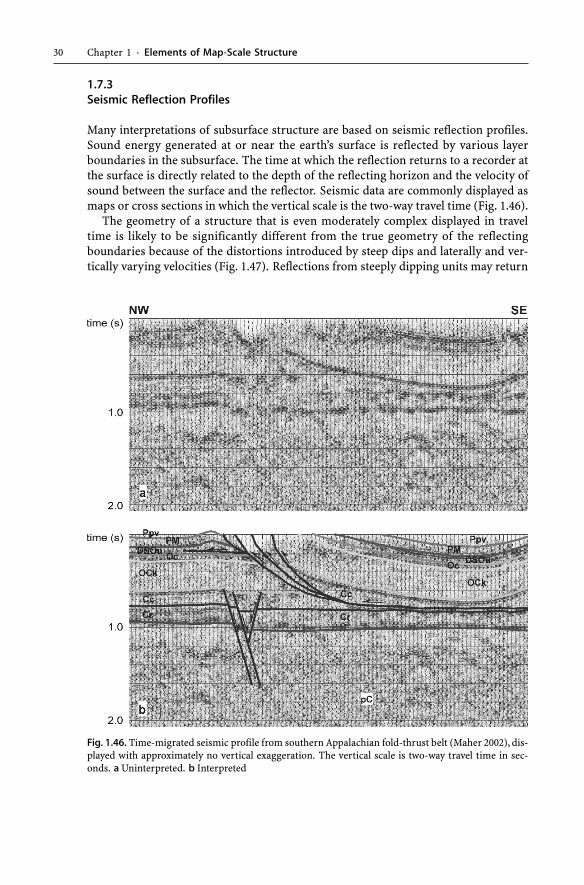
Many interpretations of subsurface structure are based on seismic reflection profiles.Sound energy generated at or near the earth’s surface is reflected by various layerboundaries in the subsurface. The time at which the reflection returns to a recorder atthe surface is directly related to the depth of the reflecting horizon and the velocity ofsound between the surface and the reflector. Seismic data are commonly displayed asmaps or cross sections in which the vertical scale is the two-way travel time (Fig. 1.46).

The geometry of a structure that is even moderately complex displayed in traveltime is likely to be significantly different from the true geometry of the reflectingboundaries because of the distortions introduced by steep dips and laterally and ver-tically varying velocities (Fig. 1.47). Reflections from steeply dipping units may return

Fig. 1.46. Time-migrated seismic profile from southern Appalachian fold-thrust belt (Maher 2002), dis-played with approximately no vertical exaggeration. The vertical scale is two-way travel time in sec-onds. a Uninterpreted. b Interpreted

31

to the surface beyond the outer limit of the recording array and so are not representedon the seismic profile. The structural interpretation of seismic reflection data requiresthe conversion of the travel times to depth. This requires an accurate model for thevelocity distribution, something not necessarily well known for a complex structure.The most accurate depth conversion is controlled by velocities measured in nearbywells (Harmon 1991).

If the trend of a seismic line is oblique to the dip of the reflector surface, two-dimen-sional reflection data have location problems similar to those of unknowingly deviatedwells. This is in addition to the location problems associated with the conversion of

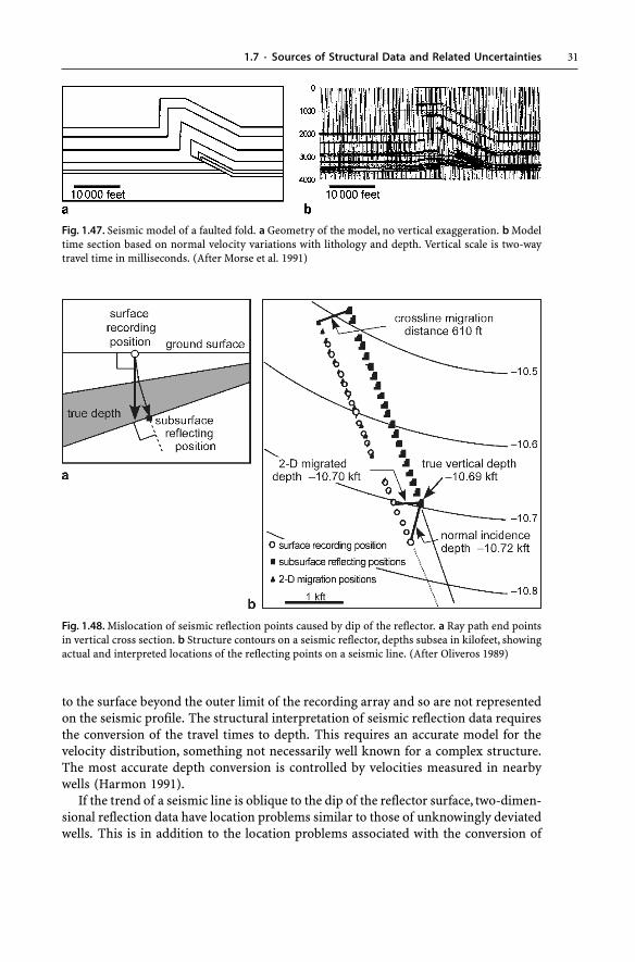
Fig. 1.47. Seismic model of a faulted fold. a Geometry of the model, no vertical exaggeration. b Modeltime section based on normal velocity variations with lithology and depth. Vertical scale is two-waytravel time in milliseconds. (After Morse et al. 1991)

Fig. 1.48. Mislocation of seismic reflection points caused by dip of the reflector. a Ray path end pointsin vertical cross section. b Structure contours on a seismic reflector, depths subsea in kilofeet, showingactual and interpreted locations of the reflecting points on a seismic line. (After Oliveros 1989)



travel time to depth. Reflections are interpreted to originate along ray paths that arenormal to the reflector boundaries (Fig. 1.48a). A normal-incidence seismic ray isdeflected up the dip (Fig. 1.48a). The true location of the reflecting point is up the dipand at a shallower depth than a point directly below the surface recording position.When the locations of reflecting points are plotted as if they were vertically below thesurface recording stations, there will be a decrease in the calculated depth (or two-waytravel time) relative to the true depth. Two-dimensional time migration is a standardprocessing procedure that corrects for the apparent dip of reflectors in the plane of theseismic line, but does not correct for the shift of the reflector positions in the true dipdirection. Two-dimensional depth migration may give the correct depth to the reflect-ing point, but still does not correct for the out-of-plane position shift. For example(Fig. 1.48b), four degrees of oblique dip leads to a 400- to 600-ft shift in the true posi-tion of the reflection points on a seismic section at depths of 10 500–10 800 ft.

elements of map-scale structure - ardiansyah kusuma … · chapter 1 elements of map-scale...

Documents