elements of electromagnetic theory, anisotropic...
TRANSCRIPT
Elements of Electromagnetic Theory, Anisotropic Media, and
Light Modulation by the Linear Electro-Optic Effect
Christophe Peucheret
DTU Fotonik
Department of Photonics Engineering
Technical University of Denmark
Abstract
The purpose of this note is to introduce the linear electro-optic effect (Pockels effect)and its applications for modulating the properties of a light wave, such as its phase, polari-sation and intensity. For this purpose, basic electromagnetic theory is first reviewed. Someelements of light propagation in an anisotropic medium are then introduced. The linearelectro-optic effect is then presented and illustrated using the classic example of KDP crys-tals. Due to its importance for modulation applications in optical communication systems,the use of lithium niobate (LiNbO3) crystals is also discussed in details. Typical electro-optic modulation configurations are introduced. Finally, transit time limitations and theirimplications for high speed modulation are also discussed.
Contents
1 Elements of electromagnetic theory 2
1.1 Maxwell’s equations . . . . . . . . . . . . . . . . . . . . . . . . . . . . . . . . . . 2
1.2 The constitutive relations . . . . . . . . . . . . . . . . . . . . . . . . . . . . . . . 3
1.3 Electromagnetic energy . . . . . . . . . . . . . . . . . . . . . . . . . . . . . . . . 5
1.4 Propagation of electromagnetic waves in an isotropic medium . . . . . . . . . . . 7
2 Light propagation in an anisotropic medium 10
2.1 Symmetry of the dielectric tensor . . . . . . . . . . . . . . . . . . . . . . . . . . . 11
2.1.1 Thermodynamic arguments . . . . . . . . . . . . . . . . . . . . . . . . . . 11
2.1.2 Principal axes of an anisotropic medium . . . . . . . . . . . . . . . . . . . 12
2.2 Propagation of a monochromatic plane wave in an anisotropic medium . . . . . . 12
2.2.1 Relative configuration of the fields . . . . . . . . . . . . . . . . . . . . . . 12
2.2.2 Energy considerations . . . . . . . . . . . . . . . . . . . . . . . . . . . . . 13
2.2.3 Eigenmodes of propagation . . . . . . . . . . . . . . . . . . . . . . . . . . 14
2.2.4 The surface of the indices . . . . . . . . . . . . . . . . . . . . . . . . . . . 15
2.3 The index ellipsoid . . . . . . . . . . . . . . . . . . . . . . . . . . . . . . . . . . . 17
2.4 Light rays in anisotropic media . . . . . . . . . . . . . . . . . . . . . . . . . . . . 21
2.4.1 The ray velocity . . . . . . . . . . . . . . . . . . . . . . . . . . . . . . . . 21
2.4.2 The ray surface . . . . . . . . . . . . . . . . . . . . . . . . . . . . . . . . . 23
2.4.3 Relation between the surfaces . . . . . . . . . . . . . . . . . . . . . . . . . 24
2.4.4 Double refraction by an anisotropic medium . . . . . . . . . . . . . . . . . 26
2.5 Summary . . . . . . . . . . . . . . . . . . . . . . . . . . . . . . . . . . . . . . . . 27
1

34153 From Photonics to Optical Communication
3 The linear electro-optic effect 28
3.1 Determination of the refractive indices under an applied electric field . . . . . . . 29
3.2 Longitudinal configuration . . . . . . . . . . . . . . . . . . . . . . . . . . . . . . . 32
3.3 Transverse configuration . . . . . . . . . . . . . . . . . . . . . . . . . . . . . . . . 34
4 Electro-optic modulation 35
4.1 The electro-optic effect in lithium-niobate . . . . . . . . . . . . . . . . . . . . . . 35
4.1.1 x-cut configuration . . . . . . . . . . . . . . . . . . . . . . . . . . . . . . . 37
4.1.2 z-cut configuration . . . . . . . . . . . . . . . . . . . . . . . . . . . . . . . 37
4.2 Light modulation . . . . . . . . . . . . . . . . . . . . . . . . . . . . . . . . . . . . 38
4.3 Phase modulation . . . . . . . . . . . . . . . . . . . . . . . . . . . . . . . . . . . 39
4.4 Polarisation modulation . . . . . . . . . . . . . . . . . . . . . . . . . . . . . . . . 40
4.5 Intensity modulation . . . . . . . . . . . . . . . . . . . . . . . . . . . . . . . . . . 42
4.5.1 Polarisation modulator followed by a polariser . . . . . . . . . . . . . . . 42
4.5.2 Interferometric structure . . . . . . . . . . . . . . . . . . . . . . . . . . . . 44
5 High frequency electro-optic modulation 45
5.1 Transit time limitation . . . . . . . . . . . . . . . . . . . . . . . . . . . . . . . . . 46
5.2 Travelling wave modulator . . . . . . . . . . . . . . . . . . . . . . . . . . . . . . . 49
Appendix A Light intensity 53
A.1 Optical intensity . . . . . . . . . . . . . . . . . . . . . . . . . . . . . . . . . . . . 53
A.2 From the electromagnetism to the communications formalisms . . . . . . . . . . 54
Appendix B On the reduction of quadratic forms 55
1 Elements of electromagnetic theory
1.1 Maxwell’s equations
The electromagnetic field consists of coupled electric and magnetic fields that are described bythe vectors E and B, known as electric and magnetic induction vectors, respectively. In orderto describe the effects of these two fundamental fields on matter, it is necessary to introduce theelectric displacement and magnetic vectors, denoted by D and H, respectively1. If the electric
current density J is also introduced, the four fields E, B, D and H are linked by Maxwell’sequations2
∇×E (r, t) = −∂B
∂t(r, t) , (1)
∇×H (r, t) = J (r, t) +∂D
∂t(r, t) , (2)
∇ ·D (r, t) = ρ (r, t) , (3)
∇ ·H (r, t) = 0, (4)
where ρ is the electric charge density and where the ∇× and ∇· notations have been usedfor the vector operators curl and div, respectively. Equations (1), (2) and (3) are known as
1Many texts introduce E and H as the fundamental fields, and D and B to describe their effect on matter.This distinction is unessential for the purpose of the present note. For a justification of this choice, one may referto e.g. Born & Wolf [1]
2James Clerk Maxwell, Edinburgh 1831 – Cambridge 1879.
2 07/10/2010

Anisotropic Media and the Linear Electro-Optic Effect
Maxwell-Faraday3 , Maxwell-Ampere4 and Maxwell-Gauss5 equations, respectively.The electric displacement can be written according to
D (r, t) = ǫ0E (r, t) +P (r, t) , (5)
where P is the electric polarisation, while the magnetic field is defined as
H (r, t) =1
µ0B (r, t)−M (r, t) , (6)
where M is the magnetisation. The constants ǫ0 and µ0 are known as the vacuum permittivity
and vacuum permeability, respectively. In order to solve Maxwell’s equations, it is necessary torelate D and H to E and B. In a conducting medium, the current density will also need tobe related to the fundamental fields. Those relations can be expressed under the most generalform as
D = D [E,B] H = H [E,B] J = J [E,B] . (7)
This set of equations are known as constitutive relations since they depend on the materialproperties. Assumptions on the material are therefore necessary in order to proceed further inthe resolution of Maxwell’s equations. In the following section, it will be shown step-by-stephow the knowledge of the material properties can be used to derive useful relations between theelectric displacement and the electric field vectors.
1.2 The constitutive relations
In this section, assumptions on the material properties are progressively introduced in order toderive explicit constitutive relations between the electric displacement and the electric field forthe types of media pertaining to this note. This is achieved by considering properties of theelectric polarisation P.
First, it is assumed that P does not depend on an applied magnetic field. Dependence on B
would lead to magneto-optic effects such as the Faraday effect, magneto-optic Kerr effect andCotton-Mouton (or Voigt) effect. The polarisation then expresses the response of the materialto an applied electric field.
Second, the material is assumed to be linear, which means that the polarisation P has alinear dependence on the electric displacement E. Assuming that P can be expanded as apower series of the electric field would lead to the field of nonlinear optics (see for instance [2]for the derivation of constitutive relations that apply when nonlinear terms can no longer beneglected). Using the formalism of linear systems, each component of the polarisation vectoron an orthonormal basis can be written
Pi (r, t) = ǫ0
∫ +∞
−∞
∫Fij
(r, r′, t, t′
)Ej
(r′, t′
)dt′dr′, (8)
where Fij is the response function of the material and the usual convention according to whichrepetition of the indices implies summation is used.
If furthermore the relation between P and E is local, i.e. P at the position r only dependson E at the same position, then the material does not exhibit spatial dispersion and
Pi (r, t) = ǫ0
∫ +∞
−∞Gij
(r; t, t′
)Ej
(r, t′)dt′. (9)
3Michael Faraday, Newington 1791 – Hampton Court 1867.4Andre-Marie Ampere, Lyon 1775 – Marseille 1836.5Carl Friedrich Gauss, Braunschweig 1777 – Gottingen 1855.
07/10/2010 3

34153 From Photonics to Optical Communication
Spatial dispersion is encountered for instance in materials that are said to be optically active.One further assumption is that the material is homogeneous, so that the relation between P
and E does not depend on the position, hence
Pi (r, t) = ǫ0
∫ +∞
−∞Tij
(t, t′)Ej
(r, t′)dt′. (10)
Finally, if time invariance is assumed,
Pi (r, t) = ǫ0
∫ +∞
−∞Rij
(t− t′
)Ej
(r, t′)dt′ = ǫ0
∫ +∞
0Rij (τ)Ej (r, t− τ) dτ, (11)
where Rij (t− t′) = Tij (t, t′) = Tij (t− t′, 0) and the assumption of causality, according to
which the effect can not be anterior to the cause, has been expressed by limiting the integrationrange in the second equality.
The convolution relation between E and P in the time domain can be expressed in a simplerform as a product in the frequency domain
Pi (r, ω) = ǫ0χij (ω) Ej (r, ω) , (12)
where Pi (r, ω) and Ej (r, ω) are the Fourier transforms of Pi (r, t) and Pi (r, t) with respect tothe time variable, and the linear susceptibility χij (ω) is the Fourier transform of the responsefunction Rij (τ). Here, the Fourier and inverse Fourier transforms between the time and angularfrequency domains are defined according to
Ei (r, ω) =
∫ +∞
−∞Ei (r, t) e
−jωtdt Ei (r, t) =1
2π
∫ +∞
−∞Ei (r, ω) e
jωtdω. (13)
Finally, (5) can be used to obtain the constitutive relation between D and E
Di (r, ω) = ǫ0 (1 + χij (ω)) Ej (r, ω) , (14)
which can also be expressed as
Di (r, ω) = ǫij (ω) Ej (r, ω) , (15)
where the elements ǫij of the permittivity tensor [ǫ] are related to the elements χij of the linearsusceptibility tensor [χ] according to
ǫij (ω) = ǫ0 (1 + χij (ω)) . (16)
It is essential at this point to keep in mind the assumptions that have led to (15): the mediumhas been assumed to be linear, homogeneous and spatially non-dispersive. Note however that(15) applies to cases where the medium is dispersive and anisotropic. Its dispersive naturecan be seen from the frequency dependence of the permittivity. This stems from the fact thatthe response of the medium is not instantaneous: P (r, t) depends on the electric displacementvector E (r, t′) at times t′ earlier than t. The tensorial nature of (15) is a consequence of theanisotropy of the medium: P depends on the direction of E.
If it is assumed that the medium is isotropic, then (15) can be replaced by the scalar relation
D (r, ω) = ǫ (ω) E (r, ω) = ǫ0ǫr (ω) E (r, ω) , (17)
where ǫr is known as the relative permittivity of the material.
4 07/10/2010

Anisotropic Media and the Linear Electro-Optic Effect
Finally, in a non dispersive medium, the permittivity does not depend on frequency andrelations of the type (15) and (17) also hold in the time domain, depending on whether themedium is anisotropic or isotropic, respectively. For an isotropic and non dispersive medium,for instance
D (r, t) = ǫ E (r, t) . (18)
Furthermore, when concerned with harmonic waves, which will be the case for most of thefollowing analysis, the frequency dependence of the material is of no importance since the waveis single frequency and the time domain relation (18) also holds at any given frequency.
At this point, a constitutive relation has been found between the electric displacement D
and the electric field E. The magnetic properties of the medium would need to be explored inorder to derive a similar relation between the magnetic field H and the magnetic induction B.Here, non magnetic materials for which M = 0 will be considered, hence
B (r, t) = µ0H (r, t) . (19)
Otherwise, for magnetic, linear, non dispersive and isotropic materials, a more general relationof the type
B (r, t) = µ0µrH (r, t) = µH (r, t) , (20)
where µr is the relative permeability, could be substituted to (19).In a conductor, the current density J can be related to the electric field according to
J (r, t) = σE (r, t) , (21)
which is a microscopic form of Ohm’s law. The proportionality factor σ is known as theconductivity of the material. Note that (21) assumes the medium to be homogeneous andisotropic, otherwise a dependence on the position r and a tensorial relation should be introducedfor σ, in a similar fashion to what has been done in the earlier study of the constitutive relationbetween E and D. In this note, the materials will be considered non-conducting, hence J = 0.
1.3 Electromagnetic energy
Using a classic vector identity6, the dot product between the electric field E and ∇×H can becalculated according to
E · [∇×H] = H · [∇×E]−∇ · [E×H] . (22)
Introducing Maxwell’s equations (1) and (2) leads to
E · ∂D∂t
+H · ∂B∂t
+∇ · [E×H] = −J · E, (23)
which can be further integrated over a volume (V ) delimited by a closed surface (Σ). Using thedivergence theorem (also known as Gauss’s theorem), which states that
∫
V(∇ · S) dV =
∮
ΣS · dΣ, (24)
the following relation is obtained
∫
V
[E · ∂D
∂t+H · ∂B
∂t
]dV = −
∫
VJ · E dV −
∮
Σ(E×H) · dΣ. (25)
6∇ · (A×B) = B · (∇×A)−A · (∇×B)
07/10/2010 5
34153 From Photonics to Optical Communication
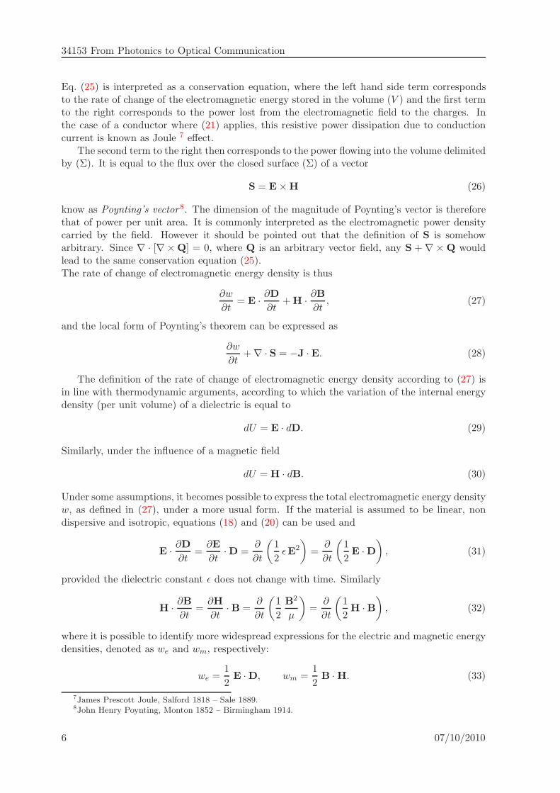
Eq. (25) is interpreted as a conservation equation, where the left hand side term correspondsto the rate of change of the electromagnetic energy stored in the volume (V ) and the first termto the right corresponds to the power lost from the electromagnetic field to the charges. Inthe case of a conductor where (21) applies, this resistive power dissipation due to conductioncurrent is known as Joule 7 effect.
The second term to the right then corresponds to the power flowing into the volume delimitedby (Σ). It is equal to the flux over the closed surface (Σ) of a vector
S = E×H (26)
know as Poynting’s vector8. The dimension of the magnitude of Poynting’s vector is thereforethat of power per unit area. It is commonly interpreted as the electromagnetic power densitycarried by the field. However it should be pointed out that the definition of S is somehowarbitrary. Since ∇ · [∇×Q] = 0, where Q is an arbitrary vector field, any S +∇ × Q wouldlead to the same conservation equation (25).The rate of change of electromagnetic energy density is thus
∂w
∂t= E · ∂D
∂t+H · ∂B
∂t, (27)
and the local form of Poynting’s theorem can be expressed as
∂w
∂t+∇ · S = −J · E. (28)
The definition of the rate of change of electromagnetic energy density according to (27) isin line with thermodynamic arguments, according to which the variation of the internal energydensity (per unit volume) of a dielectric is equal to
dU = E · dD. (29)
Similarly, under the influence of a magnetic field
dU = H · dB. (30)
Under some assumptions, it becomes possible to express the total electromagnetic energy densityw, as defined in (27), under a more usual form. If the material is assumed to be linear, nondispersive and isotropic, equations (18) and (20) can be used and
E · ∂D∂t
=∂E
∂t·D =
∂
∂t
(1
2ǫE2
)=
∂
∂t
(1
2E ·D
), (31)
provided the dielectric constant ǫ does not change with time. Similarly
H · ∂B∂t
=∂H
∂t·B =
∂
∂t
(1
2
B2
µ
)=
∂
∂t
(1
2H ·B
), (32)
where it is possible to identify more widespread expressions for the electric and magnetic energydensities, denoted as we and wm, respectively:
we =1
2E ·D, wm =
1
2B ·H. (33)
7James Prescott Joule, Salford 1818 – Sale 1889.8John Henry Poynting, Monton 1852 – Birmingham 1914.
6 07/10/2010
Anisotropic Media and the Linear Electro-Optic Effect
The electromagnetic energy density can therefore be written
w =1
2[E ·D+B ·H] , (34)
which is in total agreement with (27). It is however essential to keep in mind the assumptionsthat have led to (34), namely that the medium is isotropic and non dispersive. The case ofdispersive media will be briefly mentioned in Sect. 1.4, while it will be seen in Sect. 2 how theresults above can be extended to anisotropic media.
1.4 Propagation of electromagnetic waves in an isotropic medium
In this section, a linear, homogeneous and isotropic medium is considered and conditions sothat harmonic plane waves of the type
E (r, t) = ReE0 e
j(ωt−k·r), (35)
are solutions of Maxwell’s equations are examined9. In (35), E0 is a complex vector andRe denotes the real part. For fields that satisfy equations of the type (35), the followingsubstitutions can be made
∇ → −jk,∂
∂t→ jω, (36)
and, in the absence of charges and current sources, Maxwell’s equations (1)-(4) can be written
k×E0 = ωB0 (37)
k×H0 = −ωD0 (38)
k ·D0 = 0 (39)
k ·H0 = 0 (40)
For an harmonic wave, D0 = ǫ E0 and B0 = µH0. Using a well known vector identity10, thefollowing relation, known as Helmholtz11 equation, can be derived for E0
∇2E0 + ω2µǫ E0 = 0. (41)
An harmonic plane wave described by (35) is therefore solution of the propagation equationprovided
|k| = ω√µǫ. (42)
The surfaces of constant phase of the wave are defined by
ωt− k · r = constant (43)
9Note that it is somehow implicitly assumed here that harmonic plane waves of the type (35) could be solutions
of Maxwell’s equations. Many texts derive the well-known propagation equation ∇2E − µ0ǫ
∂2E
∂t2= 0 directly
from Maxwell’s equations for a linear, homogeneous and isotropic medium in the absence of free charges andfree currents, which is obviously satisfied by harmonic plane waves. However, in order to do so, the relationD (r, t) = ǫE (r, t) needs to be employed. It has been seen in Sect. 1.2 that this relation is correct only for anon-dispersive medium, or for an harmonic wave. Since no assumption is usually made on the dispersive natureof the medium at this stage, the harmonic nature of the solution of the propagation equation is also implicitlyassumed in those derivations.
10∇× (∇×A) = ∇ (∇ ·A)−∇2A, where ∇2 is the Laplacian operator.
11Hermann von Helmholtz, Potsdam 1821 – Charlottenburg 1894.
07/10/2010 7

34153 From Photonics to Optical Communication
and are therefore planes orthogonal to the wave vector k that defines the direction of propaga-tion. These surfaces travel at the velocity
vϕ =ω
|k| (44)
in the direction of k, which is known as the phase velocity of the wave. From (42), the phasevelocity can be expressed as a function of the permittivity and permeability of the mediumaccording to
vϕ =1√ǫµ
. (45)
In vacuum, ǫ = ǫ0, µ = µ0 and the phase velocity can be expressed as
c =1√µ0ǫ0
, (46)
which takes the well known value c = 299792458 m · s−1. In a non-magnetic medium µ = µ0
and ǫ = ǫ0ǫr = ǫ0n2, where n =
√ǫr is the refractive index of the medium, hence
vϕ =c
n. (47)
Equations (39) and (40) show that both D andH are orthogonal to the direction of propaga-tion k. Since in an isotropic medium such as the one considered here D and E are proportional,E is also perpendicular to the direction of propagation. Such a wave where E and H lie in aplane orthogonal to the direction of propagation is said to be transverse. From (37), and sinceB0 = µH0, the vector triplet (k,E0,H0) is a right handed set of orthogonal vectors whosedirections are identical to those of the orthogonal set (k,D0,B0). From (37) and (42) it can beeasily established that the magnitudes of the vectors E0 and H0 satisfy the relation
|E0||H0|
=
õ
ǫ, (48)
where the quantity η =√
µ/ǫ is known as the impedance of the medium. The impedance ofvacuum is therefore equal to η0 =
√µ0/ǫ0 ≃ 377 Ω.
From (31), (32) and (34), the electromagnetic energy density of the wave is given by
w =1
2
(ǫ E2 (r, t) +
1
µB2 (r, t)
). (49)
For an harmonic wave, the electric field can be expressed according to (35) where the complexvector E0 can be decomposed into real and imaginary vectors
E0 = E0r + j E0i. (50)
Similarly, for the magnetic induction
B0 = B0r + j B0i. (51)
Using such decompositions, the electric field is given by
E (r, t) = E0r cos (ωt− k · r)−E0i sin (ωt− k · r) (52)
8 07/10/2010

Anisotropic Media and the Linear Electro-Optic Effect
and a similar expression can be derived for B (r, t). Reporting into (49) and using the fact that
⟨cos2 (ωt− φ)
⟩=⟨sin2 (ωt− φ)
⟩=
1
2, (53)
〈cos (ωt− φ) sin (ωt− φ)〉 = 0, (54)
where 〈·〉 denotes time averaging, the time average of the electromagnetic density can be ex-pressed as
〈w〉 = 1
4
[ǫ(E2
0r +E20i
)+
1
µ
(B2
0r +B20i
)], (55)
hence finally
〈w〉 = 1
4
(ǫ |E0|2 +
1
µ|B0|2
). (56)
From (48) it can easily be established that |B0|2 = µǫ |E0|2 and therefore
〈w〉 = 1
2ǫ |E0|2 . (57)
It is important to remember at this point that the starting point for the derivation of theelectromagnetic energy density is (34), which assumes a non dispersive medium. In the caseof a dispersive material, it can be shown (see for instance [3]) that, away from absorptionresonances, the integration of (27) leads to
〈w〉 = 1
4
[∂ (ωǫ)
∂ω|E0|2 +
∂ (ωµ)
∂ω|H0|2
], (58)
which obviously simplifies to (56) when ǫ and µ are assumed to have no dependence on thefrequency (non dispersive medium).
If the Poynting vector S = E ×H is now considered, it can easily be shown using decom-positions of E0 and H0 into real and imaginary parts that its time average can be expressedaccording to
〈S〉 = 1
2Re (E0 ×H∗
0) . (59)
From the definition of the Poynting vector S = E × H, and since E and H lie in the planeorthogonal to k and are furthermore orthogonal, it is obvious that S is parallel to k. Theaverage of the Poynting vector can also be calculated from (59) by substituting (37) into (59),leading to
〈S〉 =1
2Re
(E0 ×
1
ωµ(k×E∗
0)
)(60)
=1
2ωµRe [(E0 · E∗
0)k− (E0 · k)E∗0] (61)
=1
2ωµ|E0|2 k, (62)
where the last equality stems from the facts that E0 · k = 0 according to (39) and D0 = ǫE0,as well as by definition E0 ·E∗
0 = |E0|2. Expressing the wave vector according to
k = |k|u = ω√ǫµu =
ω
vϕu = ω
n
cu, (63)
where u is an unit vector in the direction of propagation, finally leads to
〈S〉 = 〈w〉 vϕu, (64)
07/10/2010 9

34153 From Photonics to Optical Communication
plane of constant phase
Figure 1 Relative directions of the vectors and fields associated with the propagation of an harmonicplane wave in an isotropic medium.
which is in line with the interpretation of the Poynting theorem presented in Sec. 1.3 where itwas stated that the Poynting vector corresponds to the flow of electromagnetic energy.
The following properties of a plane harmonic wave propagating into an isotropic mediumshould therefore be kept in mind:
• The electric field E and electric displacement D are parallel: D = ǫE.
• The wave is transverse: both E/D and B/H lie in a plane that is perpendicular to thedirection of propagation k.
• (k,D0,B0) forms a right handed orthogonal vector triplet
• So does (k,E0,H0) since E0 and D0 are parallel, as well as H0 and B0.
• Poynting’s vector S, hence the direction of energy propagation, is oriented along thedirection of propagation of the phase k.
These essential properties are summarised in Fig. 1. It will be seen in Sec. 2 that some of thoseproperties no longer apply in anisotropic media.
2 Light propagation in an anisotropic medium
When the medium is anisotropic, the relation between the electric displacement and the electricfield becomes tensorial, as expressed in (15). Therefore the vectors D and E are no longerparallel. In the following, it will be assumed that dispersive effects can be neglected, eitherbecause the medium is non-dispersive in the frequency range of interest, or because the fieldsinvolved are monochromatic, or of a limited spectral width. In this case, a tensorial relationalso holds between D and E expressed in the time domain,
D (r, t) = [ǫ]E (r, t) , (65)
10 07/10/2010
Anisotropic Media and the Linear Electro-Optic Effect
where the dielectric tensor is denoted by [ǫ]. On an orthonormal basis (e1, e2, e3), this tensorialrelation links the components of the vectors D and E and can be expressed in a matrix formaccording to
D1
D2
D3
=
ǫ11 ǫ12 ǫ13ǫ21 ǫ22 ǫ23ǫ31 ǫ32 ǫ33
E1
E2
E3
. (66)
Such a relation is customarily also expressed as Di =∑
j ǫij Ej or using Einstein’s notation,according to which summation is performed over repeated indices, Di = ǫijEj .
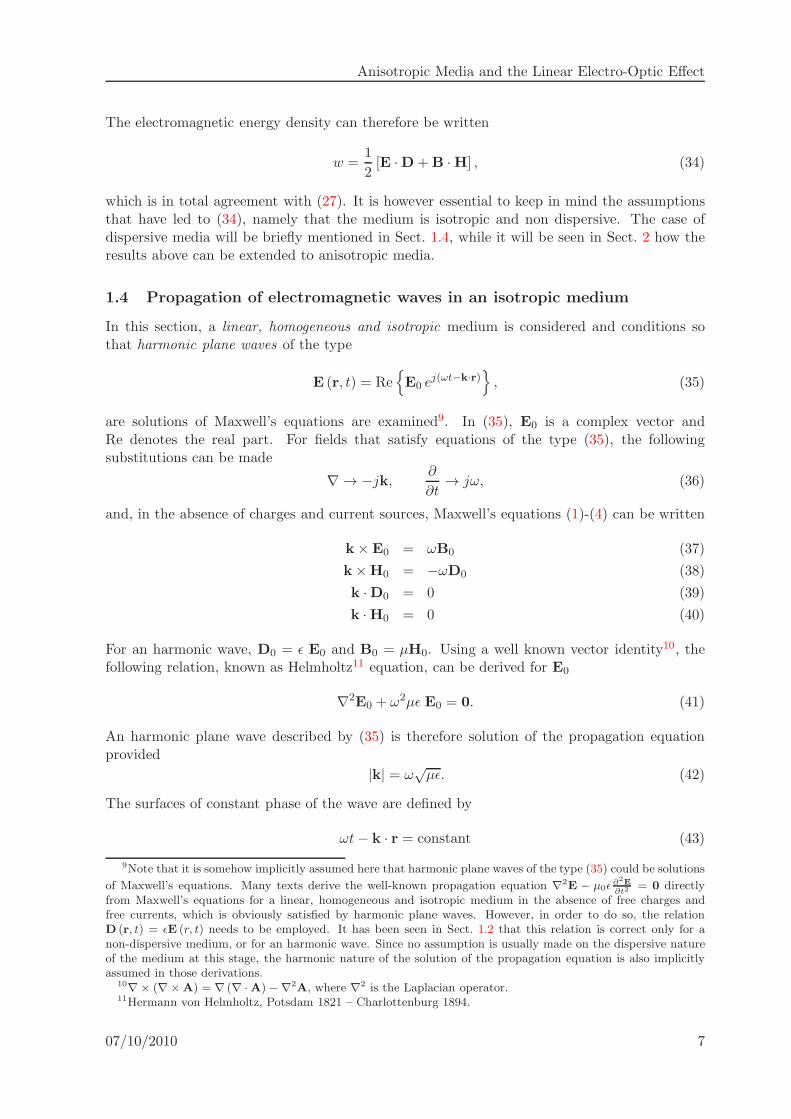
In the case of non absorbing media that are magnetically isotropic (i.e. for which B = µHwhere µ is a scalar quantity), the elements of the dielectric tensor are real quantities. Suchmaterials will be considered in this note, unless explicitly stated.
An important property of the dielectric tensor that has implications on the propagation ofelectromagnetic waves in anisotropic media is its symmetry12, i.e. ǫij = ǫji.
2.1 Symmetry of the dielectric tensor
It appears that the demonstration of the symmetry of the dielectric tensor raises some issuesin many of the popular texts, a point that has been discussed in [4]. In this section, a ther-modynamic proof of this property is first given, followed by a discussion of an often reportedattempt of derivation based on Poynting’s theorem.
2.1.1 Thermodynamic arguments
In the case of static fields, thermodynamic arguments can be used to demonstrate the symmetryof the dielectric tensor, as reported in e.g. [5, 6]. The differential of the Helmholtz free energyF of a dielectric is given by
dF = −S dT −D · dE, (67)
where S is the entropy and T denotes the temperature. This relation can be further expandedinto
dF = −S dT −∑
i
Di dEi = −S dT −∑
i
∑
j
ǫij Ej dEi, (68)
therefore
Di = − ∂F
∂Ei. (69)
Since
ǫij =∂Di
∂Ej, (70)
then
ǫij = − ∂2F
∂Ei∂Ej. (71)
However dF is a total differential. Therefore the value of ǫij as expressed in (71) should notdepend on the order of the differentiations. Consequently
ǫij = − ∂2F
∂Ei∂Ej= − ∂2F
∂Ej∂Ei= ǫji, (72)
and the dielectric tensor is symmetric.
12In the case of media whose dielectric tensor is complex, and provided the complex nature of the elementsis not due to absorption, it can be shown that the dielectric tensor exhibits Hermitian symmetry, i.e. ǫij = ǫ∗ji.This is for instance the case of media that present optical activity.
07/10/2010 11

34153 From Photonics to Optical Communication
2.1.2 Principal axes of an anisotropic medium
The dielectric tensor [ǫ] has been shown above to be symmetric and real. Therefore there existsan orthonormal basis (x,y, z) where the dielectric tensor is represented by a diagonal matrix
Dx
Dy
Dz
=
ǫx 0 00 ǫy 00 0 ǫz
Ex
Ey
Ez
, (73)
where ǫx, ǫy and ǫz are the eigenvalues of [ǫ]. The directions determined by x, y and z are knowas the principal axes of the medium. In analogy with the isotropic case, refractive indices canbe defined along the three principal axes according to ni =
√ǫi/ǫ0, where i = x, y, z.
2.2 Propagation of a monochromatic plane wave in an anisotropic medium
In this section, the propagation of a monochromatic plane wave with frequency ω and wavevector k in an anisotropic medium defined by its dielectric tensor [ǫ] is considered. The electricdisplacement of the plane wave can be expressed in complex notation according to
D (r, t) = ReD0 e
j(ωt−k·r)
(74)
where D0 is a complex vector that describes the state of polarisation of the wave. The fields E,B and H can be expressed in a similar way. In analogy with the isotropic case, the wave vectorcan be written
k = ωn
cu (75)
where u is a unit vector in the direction of the wave vector k and the physical meaning of nwill be clarified. As in the isotropic case, u is orthogonal to the planes of constant phase anddefines the direction of the wave normal.
In the following, the conditions for such a plane wave to propagate undistorted in thedielectric medium are examined.
2.2.1 Relative configuration of the fields
For such a monochromatic plane wave, the substitution ∂∂t → jω and ∇ → −jω n
cu can beperformed into Maxwell’s equations (1)-(4), leading to
n
cu×E = B (76)
1
µ0
n
cu×B = −D (77)
u ·D = 0 (78)
u ·B = 0 (79)
In deriving (79) it has been further assumed that the medium is non magnetic, M = 0, henceB = µ0H. Under this assumption, the Poynting vector becomes
S = E× B
µ0. (80)
Considering eq. (76)-(80) above, it can easily be established that, at any given time
• (u,D,B) is a right handed orthogonal vector triplet.
12 07/10/2010
Anisotropic Media and the Linear Electro-Optic Effect
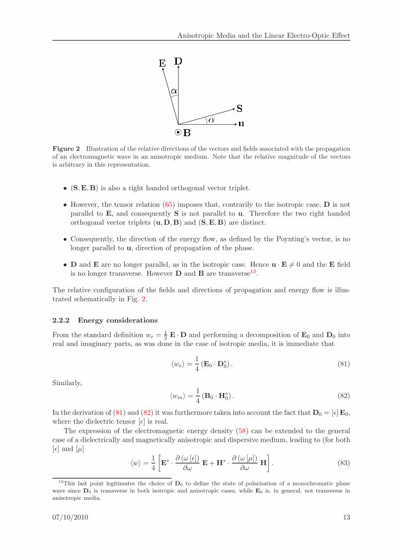
Figure 2 Illustration of the relative directions of the vectors and fields associated with the propagationof an electromagnetic wave in an anisotropic medium. Note that the relative magnitude of the vectorsis arbitrary in this representation.
• (S,E,B) is also a right handed orthogonal vector triplet.
• However, the tensor relation (65) imposes that, contrarily to the isotropic case, D is notparallel to E, and consequently S is not parallel to u. Therefore the two right handedorthogonal vector triplets (u,D,B) and (S,E,B) are distinct.
• Consequently, the direction of the energy flow, as defined by the Poynting’s vector, is nolonger parallel to u, direction of propagation of the phase.
• D and E are no longer parallel, as in the isotropic case. Hence u · E 6= 0 and the E fieldis no longer transverse. However D and B are transverse13.
The relative configuration of the fields and directions of propagation and energy flow is illus-trated schematically in Fig. 2.
2.2.2 Energy considerations
From the standard definition we =12 E ·D and performing a decomposition of E0 and D0 into
real and imaginary parts, as was done in the case of isotropic media, it is immediate that
〈we〉 =1
4(E0 ·D∗
0) . (81)
Similarly,
〈wm〉 = 1
4(B0 ·H∗
0) . (82)
In the derivation of (81) and (82) it was furthermore taken into account the fact thatD0 = [ǫ]E0,where the dielectric tensor [ǫ] is real.
The expression of the electromagnetic energy density (58) can be extended to the generalcase of a dielectrically and magnetically anisotropic and dispersive medium, leading to (for both[ǫ] and [µ]
〈w〉 = 1
4
[E∗ · ∂ (ω [ǫ])
∂ωE+H∗ · ∂ (ω [µ])
∂ωH
]. (83)
13This last point legitimates the choice of D0 to define the state of polarisation of a monochromatic planewave since D0 is transverse in both isotropic and anisotropic cases, while E0 is, in general, not transverse inanisotropic media.
07/10/2010 13

34153 From Photonics to Optical Communication
2.2.3 Eigenmodes of propagation
In this section, the solutions of the propagation equation in an anisotropic medium are studiedin more details. In particular it will be shown that, for a given direction of propagation,two linearly polarised plane waves with well defined polarisations can maintain their state ofpolarisation over propagation in the medium. These so-called eigenmodes of propagation, andassociated phase velocities, or equivalently refractive indices, will be derived in this section, andtheir main characteristics will be examined.
Substituting (76) into (77) enables to solve Maxwell’s equations for the electric displace-ment14
D =n2
c2µ0[E− (u · E)u] . (84)
Therefore, two alternative expressions relating the electric displacement D to the electric fieldvector E have been found. The first one stems from the constitutive relation (65), while thesecond one is a consequence of Maxwell’s equations. Those two relations can be expressed in acoordinate system that coincides with the principal axes of the dielectric tensor, leading to
Di = ǫ0n2iEi, (85)
and
Di =n2
c2µ0[Ei − (u ·E) ui] . (86)
Eliminating Di between the two equations and recalling that c = 1/√ǫ0µ0,
Ei =n2
n2 − n2i
(u ·E) ui, (87)
hence
u · E =∑
i
uiEi =∑
i
n2 (u · E)
n2 − n2i
u2i , (88)
and finally∑
i
u2in2 − n2
i
=1
n2. (89)
Using the fact that∑
u2i = 1, since u is a unit vector, enables to obtain the alternativeexpression
∑
i
n2iu
2i
n2 − n2i
= 0, (90)
∑
i
u2i1n2 − 1
n2i
= 0, (91)
and∑
i
u2iv2ϕ − v2i
= 0, (92)
where vϕ = c/n and vi = c/ni. Eq. (89)-(92) are known as alternative forms of Fresnel’sequation of wave normal15. They enable the determination of n, or equivalently vϕ, once thedirection of the wave normal u is known.
14 07/10/2010
Anisotropic Media and the Linear Electro-Optic Effect
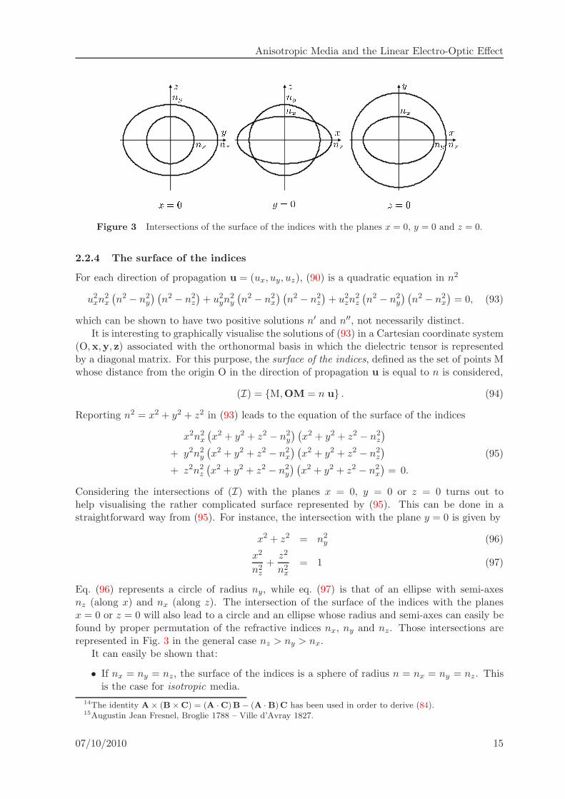
Figure 3 Intersections of the surface of the indices with the planes x = 0, y = 0 and z = 0.
2.2.4 The surface of the indices
For each direction of propagation u = (ux, uy, uz), (90) is a quadratic equation in n2
u2xn2x
(n2 − n2
y
) (n2 − n2
z
)+ u2yn
2y
(n2 − n2
x
) (n2 − n2
z
)+ u2zn
2z
(n2 − n2
y
) (n2 − n2
x
)= 0, (93)
which can be shown to have two positive solutions n′ and n′′, not necessarily distinct.It is interesting to graphically visualise the solutions of (93) in a Cartesian coordinate system
(O,x,y, z) associated with the orthonormal basis in which the dielectric tensor is representedby a diagonal matrix. For this purpose, the surface of the indices, defined as the set of points Mwhose distance from the origin O in the direction of propagation u is equal to n is considered,
(I) = M,OM = n u . (94)
Reporting n2 = x2 + y2 + z2 in (93) leads to the equation of the surface of the indices
x2n2x
(x2 + y2 + z2 − n2
y
) (x2 + y2 + z2 − n2
z
)
+ y2n2y
(x2 + y2 + z2 − n2
x
) (x2 + y2 + z2 − n2
z
)
+ z2n2z
(x2 + y2 + z2 − n2
y
) (x2 + y2 + z2 − n2
x
)= 0.
(95)
Considering the intersections of (I) with the planes x = 0, y = 0 or z = 0 turns out tohelp visualising the rather complicated surface represented by (95). This can be done in astraightforward way from (95). For instance, the intersection with the plane y = 0 is given by
x2 + z2 = n2y (96)
x2
n2z
+z2
n2x
= 1 (97)
Eq. (96) represents a circle of radius ny, while eq. (97) is that of an ellipse with semi-axesnz (along x) and nx (along z). The intersection of the surface of the indices with the planesx = 0 or z = 0 will also lead to a circle and an ellipse whose radius and semi-axes can easily befound by proper permutation of the refractive indices nx, ny and nz. Those intersections arerepresented in Fig. 3 in the general case nz > ny > nx.
It can easily be shown that:
• If nx = ny = nz, the surface of the indices is a sphere of radius n = nx = ny = nz. Thisis the case for isotropic media.
14The identity A× (B×C) = (A ·C)B− (A ·B)C has been used in order to derive (84).15Augustin Jean Fresnel, Broglie 1788 – Ville d’Avray 1827.
07/10/2010 15

34153 From Photonics to Optical Communication
−3
−2
−1
0
1
2
3
0 1
2 3
−2
−1
0
x
y
z
Figure 4 Representation of the surface of the indices for y ≥ 0 and z ≤ 0 in the arbitrary case nx = 1,ny = 2, nz = 3. The two shells of the surface are clearly visible, as well as their intersection in the planey = 0.
• If two out of the three indices are equal, by convention nx = ny, the surface of the indicesis constituted of a sphere and an ellipsoid of revolution around the axis (O, z). The sphereand ellipsoid are tangent at their intersection with the (O, z) axis. The medium is saidto be uniaxial. For historical reasons, nx = ny is known as the ordinary index no and nz
is the extraordinary index ne. If furthermore no > ne the medium is said to be negative,while it is described as positive when ne > no.
• In the more general case where all three indices are different, and using the convention nz >ny > nx, the surface is constituted of two shells whose intersections can be determinedby considering their intersection with the y = 0 plane (since nz > ny > nx the two shellsdo not intersect in the x = 0 and z = 0 planes, and have four intersection points in they = 0 plane). In this case the medium is said to be biaxial. An example of surface of theindices for a biaxial medium is represented in Fig. 4. In order to emphasize its shape inthe most general case, it has been represented for arbitrary values of the indices nx = 1,ny = 2 and nz = 3. The intersection points between the two shells in the plane y = 0 canbe clearly seen.
Consequently, it has been shown that, for any given direction of the wave normal u thereexists at most two allowed positive values for n. Those values are found by considering theintersection of the direction u with the two shells constituting the surface of the indices. In thecase of propagation along the z direction in an uniaxial crystal, those two values reduce to asingle index no. This is also the case for specific propagation directions corresponding to theintersections between the shells of the surface of the indices in a biaxial crystal. The directionsof propagation for which only a single value of n can be found are known as the optic axes.Hence the denomination of uniaxial and biaxial media. Apart in the case of propagation alongan optic axe, two harmonic plane waves characterised by their displacement D′ and D′′ andtheir phase velocity v′ϕ = c/n′ and v′′ϕ = c/n′′ can be associated with n′ and n′′, respectively.It will be shown in Sec. 2.3 that D′ and D′′ correspond to two orthogonal linearly polarised
16 07/10/2010

Anisotropic Media and the Linear Electro-Optic Effect
waves.The discussion above has been based on the use of the surface of the indices (94). Other
relevant geometric constructions are often considered in the literature. The k-vector surface(K) = K,OK = k is obviously homothetic to (I). Another frequent choice16 is that of thenormal surface, defined as
(N ) = P,OP = vϕ u , (98)
which directly enables the determination of vϕ for a given direction of the wave normal u.
In summary:
• For each direction of the wave normal u there exists two allowed refractive indices n′
and n′′ that are solutions of Fresnel’s equation and that can be found by consideringthe intersection of the surface of the indices with the direction of u. These two indicesreduce to one in some pathological cases.
• Two plane waves characterised by their displacement vectors D′ and D′′ can be asso-ciated to n′ and n′′, respectively. These two waves are known as the eigenmodes ofpropagation in the direction of the wave normal u.
• Those two waves are linearly polarised and preserve their linear polarisation over prop-agation in the medium.
• Furthermore their displacement vectors D′ and D′′ are orthogonal and are also orthog-onal to the direction of propagation u.
• Since both D′ and D′′ are orthogonal to u, the orthogonal vector triplet (u,D′,D′′)can be used to decompose arbitrary waves propagating along u in the medium.
So far the use of the surface of the indices has enabled the determination of the refractiveindices n′ and n′′, or equivalently the phase velocities v′ϕ and v′′ϕ, but does not provide directlyusable information on the associated eigenmodes D′ and D′′. It will be shown in the nextsection that the properties of the eigenmodes, including the orientation of their D vector, canbe determined in a straightforward manner based on a powerful geometrical construction knownas the index ellipsoid.
2.3 The index ellipsoid
The tensor relation between the electric field E and the displacement D in an anisotropicmedium has been introduced in (65) and can be expressed in an alternative form as
D = ǫ0 [ǫr]E, (99)
where [ǫr] is the relative dielectric tensor. It is convenient to introduce the impermeabilitytensor [η] defined by
ǫ0E = [η]D. (100)
The impermeability tensor is the inverse of the relative dielectric tensor
[η] = [ǫr]−1 . (101)
16Interestingly, the French literature seems to favour the use of the surface of the indices, while English textstend to use the normal surface.
07/10/2010 17

34153 From Photonics to Optical Communication
Figure 5 Illustration of the relative configuration of the vectors in (103).
Since [ǫ] is symmetric, [η] is also symmetric and both tensors have the same principal axes. Inthe orthonormal basis (x,y, z) where [ǫ] is diagonal, [η] is also diagonal and can be expressedas
[η] =
1n2x
0 0
0 1n2y
0
0 0 1n2z
. (102)
Reporting (100) into (84)
[η]D− u · [η]Du =1
n2D (103)
The left hand side of (103) represents the projection of the vector [η]D on a plane that isorthogonal to u. The relative configuration of the vectors in (103) is illustrated in Fig. 5.It is therefore natural to introduce a new orthonormal basis (i, j,u) where i and j are twoorthonormal vectors in the plane orthogonal to u. Representing the impermeability tensor by(ηij) with i, j = 1, 2, 3, in this basis and recalling that D is orthogonal to u immediately leadsto (
ηii ηijηji ηjj
)D =
1
n2D. (104)
This is a standard eigenvalue equation with 1/n2 as eigenvalue and D as eigenvector. Since(ηij) is symmetric and real, its eigenvalues are real and its eigenvectors associated to twodifferent eigenvalues D′ and D′′ are real and orthogonal. Consequently, the solutions of thepropagation equation in a linear anisotropic medium are two linearly polarised planes waves thatare furthermore orthogonal. These solutions are known as the two normal modes of propagation,to which two refractive indices, n′ and n′′ can be associated, respectively. n′ and n′′ can befound by solving the eigenvalue equation
det
[ηt −
1
n2I
]= 0, (105)
where ηt is sometimes described as the transverse impermeability tensor, represented by (ηij)(with i, j = 1, 2) in the basis (i, j) of the plane orthogonal to u, and I is the identity matrix.Not surprisingly, solving the eigenvalue equation (105) will lead to Fresnel’s equation alreadystudied in Sec. 2.2.
A geometric construction that enables to find the normal modes and the associated refractiveindices for a given propagation direction is now introduced. The surface (E) defined by the pointsM such that |OM| = n, where n is the refractive index in the direction of propagation u, andthe direction of the vector OM is that of the vector D is considered. Mathematically, thissurface is defined as
(E) =M,OM = n
D
|D|
. (106)
18 07/10/2010
Anisotropic Media and the Linear Electro-Optic Effect
Recalling equation (84)
D =n2
c2µ0[E− (u · E)u] , (107)
immediately leads to
D2 =n2
c2µ0E ·D (108)
since u and D are orthogonal. In the orthonormal basis (x,y, z) where [ǫ] is diagonal, (85) alsoapplies and
Di = ǫ0n2iEi. (109)
Hence
|D|2 = n2
c2µ0
∑
i
D2i
ǫ0n2i
, (110)
and therefore∑
i
1
n2i
(nDi
|D|
)2
= 1, (111)
where, according to the definition of (E), the nDi/ |D| correspond to the coordinates of thevector OM = (X,Y,Z) in the orthonormal basis (x,y, z). Eq. (111) can be expressed as afunction of X, Y , Z, leading to
X2
n2x
+Y 2
n2y
+Z2
n2z
= 1, (112)
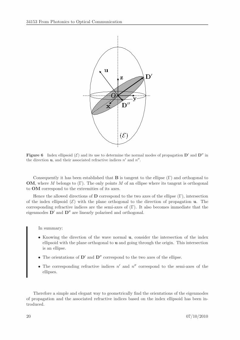
which is the equation of an ellipsoid expressed in its principal axes and whose semi-axes are oflengths nx, ny and nz. This ellipsoid is known as index ellipsoid or optical indicatrix and isschematically represented in Fig. 6.
It is now shown how the index ellipsoid can be used to determine the directions of the eigen-polarisations D′ and D′′, as well as their associated refractive indices. The electric displacementD is known to lie in the plane orthogonal to the direction of propagation u. Consequently, basedon the definition of the surface (E), the extremity M of the vector OM associated to D belongsto the intersection of the index ellipsoid with the plane orthogonal to u, which is an ellipse (Γ)of center O. Let n be the unit vector orthogonal to the ellipsoid (E) in M . n can be expressedin the basis (x,y, z) by17:
n ∝
Xn2x
Yn2y
Zn2z
(113)
In the basis (x,y, z), Ei = Di/ǫ0n2i and, by definition, OM = nD/ |D|. Consequently,
E =|D|nǫ0
Xn2x
Yn2y
Zn2z
, (114)
and therefore n is parallel to E. It is also known that B lies in the plane orthogonal to u andthat B is orthogonal to E. Since B is orthogonal to E, B lies in the plane that is tangent to(E) in M . As B lies in the plane orthogonal to u, necessarily B is tangent to the ellipse (Γ).From Maxwell’s equations, B is also known to be orthogonal to D.
17The normal to a surface defined by f (x, y, z) = 0 is proportional to the vector ∇f =(
∂f
∂x, ∂f
∂y, ∂f
∂z
)
07/10/2010 19
34153 From Photonics to Optical Communication
O
x
Figure 6 Index ellipsoid (E) and its use to determine the normal modes of propagation D′ and D′′ inthe direction u, and their associated refractive indices n′ and n′′.
Consequently it has been established that B is tangent to the ellipse (Γ) and orthogonal toOM, where M belongs to (Γ). The only points M of an ellipse where its tangent is orthogonalto OM correspond to the extremities of its axes.
Hence the allowed directions of D correspond to the two axes of the ellipse (Γ), intersectionof the index ellipsoid (E) with the plane orthogonal to the direction of propagation u. Thecorresponding refractive indices are the semi-axes of (Γ). It also becomes immediate that theeigenmodes D′ and D′′ are linearly polarised and orthogonal.
In summary:
• Knowing the direction of the wave normal u, consider the intersection of the indexellipsoid with the plane orthogonal to u and going through the origin. This intersectionis an ellipse.
• The orientations of D′ and D′′ correspond to the two axes of the ellipse.
• The corresponding refractive indices n′ and n′′ correspond to the semi-axes of theellipses.
Therefore a simple and elegant way to geometrically find the orientations of the eigenmodesof propagation and the associated refractive indices based on the index ellipsoid has been in-troduced.
20 07/10/2010

Anisotropic Media and the Linear Electro-Optic Effect
2.4 Light rays in anisotropic media
So far it has been demonstrated that anisotropic media support two orthogonal eigenmodes,each with its own phase velocity and polarisation. The values of the phase velocities and theorientations of the D vectors of the eigenmodes can be easily retrieved, for a given direction ofthe wave normal u. Historically, the observation of double images through a crystal of calcitehas been reported as early as 1669 by Erasmus Bartholin18 in his famous book “Experimenta
crystalli Islandici disdiaclastici quibus mira & insolita refractio detegitur” (Copenhagen, 1669).This effect, which is now known to be a manifestation of light propagation in an anisotropicmedium, has been puzzling several generation of scientists including Newton, Huygens andFresnel. It has also been instrumental in establishing the wave theory of light, including thetransverse nature of light vibrations and the concept of polarisation.
The theory that has been developed so far in this note does not enable yet the explanationof the formation of double images (also known as double refraction) by an anisotropic crystal.For this purpose it is essential to clarify the nature and properties of rays of light propagatingin an anisotropic medium. In this section, the concept of ray velocity will be introduced. A newsurface enabling its determination for a given ray direction will be presented, and its relationwith the surface of the indices will be analysed. In particular, it will be shown that the lightrays, which follow the direction of Poynting’s vector, are orthogonal to the surface of the indices.Finally, the effect of double refraction will be clarified.
2.4.1 The ray velocity
In analogy with (64), derived in the case of isotropic media, the ray velocity vr is defined in thecase of anisotropic media as
〈S〉 = 〈w〉 vr s, (115)
where s is an unit vector in the direction of Poynting’s vector S.
Based on the expressions of the electric and magnetic energy densities (33), as well as onMaxwell’s equations (76) and (77), and using the expression of the scalar triple product19, thefollowing expressions are obtained:
E ·D = − 1
µ0
n
cE · (u×B) =
1
µ0
n
cu · (E×B) , (116)
and
H ·B =1
µ0
n
cB · (u×E) =
1
µ0
n
cu · (E×B) . (117)
Hence the electromagnetic energy density
w =n
cu ·(E× B
µ0
)=
n
cu · S. (118)
From (115), and since u · s = cosα, the ray velocity can be expressed as a function of the phasevelocity vϕ = c/n as
vϕ = vr cosα. (119)
It is also possible to define a ray index nr such that vr = c/nr, which can be related to naccording to
nr = n cosα. (120)
18Erasmus Bartholin, Roskilde 1625 – Copenhagen 1698.19A · (B×C) = B · (C×A) = C · (A×B).
07/10/2010 21

34153 From Photonics to Optical Communication
Equation (119) shows that the phase velocity is the projection of the ray velocity on the directionof the wave normal.
Equation (115) has important implications in the context of geometrical optics. The lightrays follow the direction of Poynting’s vector, hence that of the unit vector s. The ray indexis therefore the one that needs to be considered in the framework of ray optics. An importantissue in the understanding of double refraction is the practical determination of the directionof the light rays in an anisotropic medium, a problem which will be addressed in Sec. 2.4.3.
It can furthermore be shown that, in case the medium is dispersive, the ray velocity can beidentified with the group velocity. Starting from Maxwell’s equations
k×E = ωµ0H, (121)
k×H = −ωD, (122)
infinitesimal variations of the wave vector δk and of the frequency δω will result in variationsof the fields δE, δH and δD, that can be expressed from (121) and (122) as
δk×E+ k× δE = δωµ0 H+ ωµ0 δH (123)
and
δk ×H+ k× δH = −δω D− ω δD. (124)
Performing the scalar product of (123) by H and using the properties of the triple scalar product(see footnote 19) leads to
δk · (E×H) + k · (δE ×H)− ωµ0 H · δH = δωµ0 H2, (125)
where, using Maxwell’s equation (121), the following substitution can be made
− ωµ0 H · δH = − (k×E) · δH = −k · (E× δH) , (126)
finally resulting in
δk · (E×H) + k · (δE×H)− k · (E× δH) = δωµ0 H2. (127)
Similarly, multiplying (124) by E results in
− δk · (E×H)− k · (E× δH) + ω δD · E = −δω D ·E. (128)
Furthermore, since the dielectric tensor is symmetric, it is straightforward that
δD ·E = D · δE, (129)
hence
ω δD · E = ω D · δE = − (k×H) · δE = k · (δE×H) (130)
where Maxwell’s equation (122) and the usual scalar triple product have been used. Finally
− δk · (E×H)− k · (E× δH) + k · (δE ×H) = −δω D · E. (131)
Subtracting (131) from (127) finally leads to
2δk · (E×H) = δω(µ0H
2 +D · E), (132)
22 07/10/2010

Anisotropic Media and the Linear Electro-Optic Effect
which can be simply expressed asδk · S = δω w (133)
The group velocity of the wave packet is equal to20
vg = ∇kω, (134)
henceδω = ∇kω · δk = vg · δk. (135)
Using (115), (133) and (135), it is immediate that the group velocity is equal to the ray velocity21
vg = vr s. (136)
2.4.2 The ray surface
It has been shown in Sect. 2.2.3 how the existence of two alternative relations expressing thedisplacement D as a function of the electric field E, one based on the constitutive relation(65), the other stemming from Maxwell’s equations (84), led to the definition of the surfaceof the indices, once expressed in a coordinate system coinciding with the principal axes of thedielectric tensor. This surface of the indices enables the geometric determination of the possiblevalues of n for a given direction of propagation, as defined by the wave normal u.
The problem of interest here is to determine the allowed values of the ray index nr for aparticular ray direction s. It is now shown how a geometric construction of the same type asthat of the surface of the indices can be introduced in order to solve this problem. The vector
D⊥ = D− (s ·D) s (137)
is the projection of D on the plane orthogonal to s. Based on the relative configuration of thefields represented in Fig. 2, this vector is parallel to E. It can therefore also be expressed as afunction of the unit vector in the direction of E as
D⊥ =
(D · E
|E|
)E
|E| , (138)
where the scalar product between D and E can be calculated from (84), leading to
D ·E =n2
c2µ0
[|E|2 − (u ·E)2
](139)
=n2
c2µ0|E|2
[1− cos2 (u,E)
], (140)
which, after some further arithmetics leads to
D · E =n2
c2µ0|E|2 cos2 α =
n2r
c2µ0|E|2 . (141)
Therefore (138) becomes
D⊥ =n2r
c2µ0E. (142)
20Equation (134) is simply a generalisation of the well known expression vg = ∂ω∂k
that applies to a wave packet
of the type E (z, t) = Re
∫ +∞
−∞A (k) ej(ωt−kz)dk
to the case of a 3 dimensional wave packet.21In the case of magnetic anisotropy, the same conclusion would have been reached. The starting point would
have been k×E = ωB and the symmetry of the magnetic permeability tensor [µ] would have been used.
07/10/2010 23
34153 From Photonics to Optical Communication
The two alternative expression for D⊥, (137) and (142) finally lead to
E =c2µ0
n2r
[D− (s ·D) s] . (143)
Another relation linking D to E is of course the constitutive relation
E = [ǫ]−1D, (144)
which can be written in in a coordinate system coinciding with the principal axes of the dielectrictensor as
Ei =1
ǫ0 n2i
Di. (145)
It can be observed that (84) and (143) are similar equations that can be obtained one from theother by making the substitutions
D ↔ E u ↔ s µ0 ↔1
µ0vϕ ↔ 1
vrn ↔ 1
nr. (146)
Consequently, in the same way as Fresnel’s equations, which enable the determination of possiblevalues of n or vϕ for a given direction of the wave normal u, had been established from (84)and (85), (143) and (145) will lead to quadratic equations enabling the determination of nr, orequivalently vr, for a given ray direction s. Such relations can be expressed as
∑
i
s2i1v2r
− 1v2i
= 0, (147)
∑
i
v2i s2i
v2r − v2i= 0, (148)
and∑
i
s2in2r − n2
i
= 0. (149)
Geometric constructions, which are the counterparts of the surface of the indices (94) and ofthe normal surface (98), can be introduced to visualise the solutions of the Fresnel equationsfor the ray indices or ray velocities. The ray surface is defined as
(R) = Q,OQ = vr s . (150)
It is also possible to define a surface of ray indices according to
(S) = N,ON = nr s . (151)
It will be shown in the next section how the ray surface and the surface of the ray indices relateto the normal surface and the surface of the indices.
2.4.3 Relation between the surfaces
The surface of the indices has been defined in (94) as the the locus of point M such thatOM = nu. Defining the vector n such that n = nu, this surface can expressed by an implicitequation of the form f (n) = 0, or equivalently g (k, ω) = 0 where g (k, ω) = f (ck/ω). The
24 07/10/2010
Anisotropic Media and the Linear Electro-Optic Effect
normal to the surface of the indices at a point M is proportional to the gradient of f withrespect to n at this point, i.e. to ∇nf . Since g (k, ω) = 0, its differential dg is equal to zero
dg = ∇kg · dk+∂g
∂ωdω = 0. (152)
The group velocity is equal tovg = ∇kω, (153)
hencedω = ∇kω · dk = vg · dk. (154)
Reporting into (152), the following relation is obtained
(∇kg +
∂g
∂ωvg
)· dk = 0. (155)
Substituting
∇kg =c
ω∇nf, (156)
and∂g
∂ω= ∇nf · ∂n
∂ω= − 1
ωn · ∇nf (157)
into (155) leads to (c
ω∇nf − 1
ωn · ∇nf vg
)· dk = 0, (158)
from which the group velocity can be expressed according to
vg = c∇nf
n · ∇nf. (159)
Since it has been shown in (136) that the group velocity vector is parallel to s, it can beconcluded that s is parallel to the gradient of f with respect to n, hence to the normal to thesurface of the indices.
The direction of the rays for a given direction of the wave normal u is parallel to thenormal to the surface of the indices at its intersection point with the direction defined by u.
This property is of a high practical importance since it enables the determination of thedirections of the light rays in an anisotropic medium, once the direction of the wave normal isknown. It will be shown that continuity conditions at the interface between two media enablethe determination of the wave normal direction. However, this direction is only of theoreticalinterest since it cannot be observed directly in experiments. On the other hand, the directionof the light rays can be directly related to experimental observations.
Taking into account the duality property between the ray surface and the surface of theindices (146), it can also be shown that the direction of u is that of the normal to the raysurface at its intersection with the ray direction s.
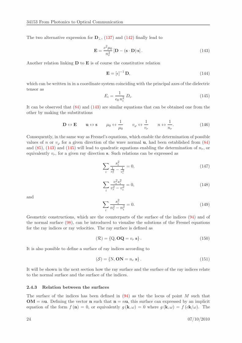
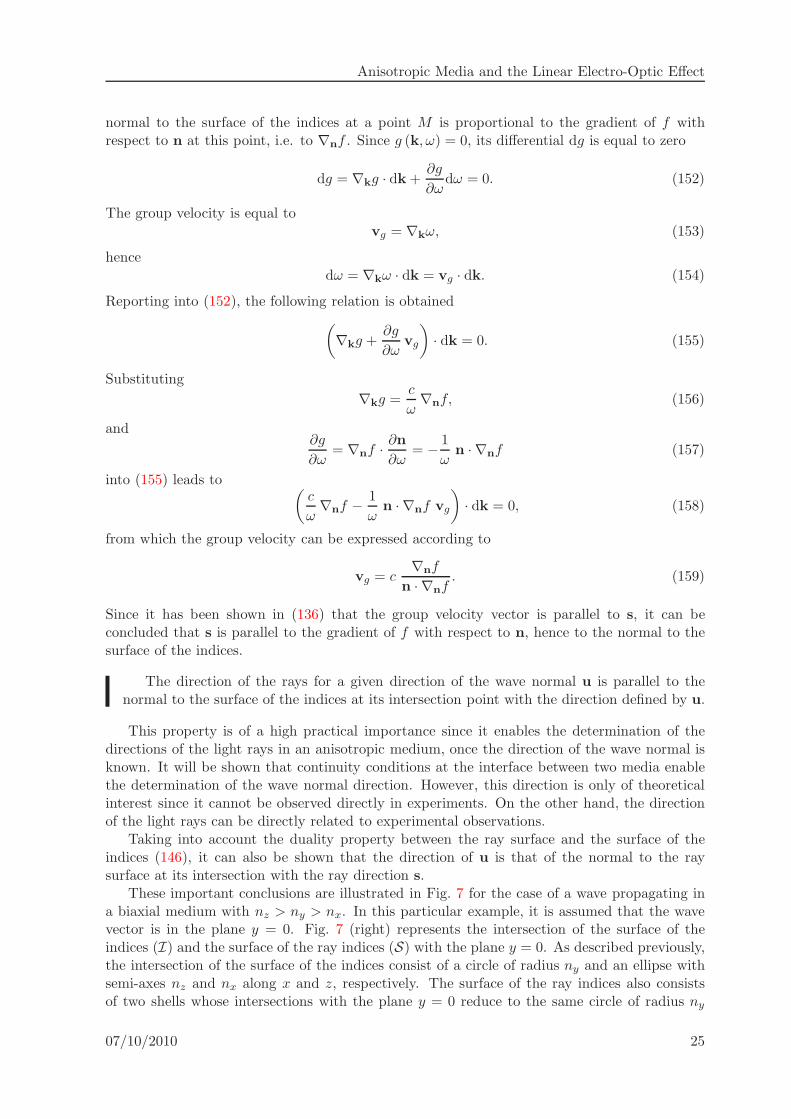
These important conclusions are illustrated in Fig. 7 for the case of a wave propagating ina biaxial medium with nz > ny > nx. In this particular example, it is assumed that the wavevector is in the plane y = 0. Fig. 7 (right) represents the intersection of the surface of theindices (I) and the surface of the ray indices (S) with the plane y = 0. As described previously,the intersection of the surface of the indices consist of a circle of radius ny and an ellipse withsemi-axes nz and nx along x and z, respectively. The surface of the ray indices also consistsof two shells whose intersections with the plane y = 0 reduce to the same circle of radius ny
07/10/2010 25
34153 From Photonics to Optical Communication
velocities indices
Figure 7 Relations between the normal surface and the ray surface (left) and between the surface ofthe indices and the surface of the ray indices (right). The general case of a a biaxial medium is consideredhere. The intersections of the various surfaces with the plane y = 0 are represented.
and a more complex curve that also intersects the axes (Ox) and (Oy) at distances nz and nx
from the origin, respectively. First, the focus is on the intersection of the wave normal with theellipse. It has just been established that s is parallel to the normal to the surface of the indicesat its intersection M with the direction u. The vector s is therefore orthogonal to the tangentto the ellipse at M . Hence the corresponding point N on the surface of the ray velocities, whichis defined by its intersection with the tangent to the ellipse at M . The ray direction is that ofON and the corresponding ray index is given by the distance |ON|. It thus becomes possible togeometrically determine the ray direction and the ray index once the direction of wave normalis known. In the case of the intersection of the wave normal direction with the circle of radiusny, the directions defined by u and s are identical and nr = n.
In a similar fashion it is possible to determine the ray direction from the wave normaldirection using the ray surface (R) and the normal surface (N ), as represented in Fig. 7 (left).Since u is normal to (R) at its intersection Q with the ray direction s, the direction of s can befound by considering the intersection of the plane orthogonal to u at P and the ray surface (R).This plane is tangent to (R) at Q, which therefore defines the ray direction and the ray velocityaccording to OQ = vrs. It is important to observe at this point that all this discussion appliesto the general case of a biaxial medium provided the direction of the wave normal does notcoincide with an optical axis (i.e. the vector u is not directed towards the intersection betweenthe circle and the ellipse defining the intersection of the surface of the indices with the planey = 0). This situation would give rise to a peculiar behaviour known as conical refraction.
2.4.4 Double refraction by an anisotropic medium
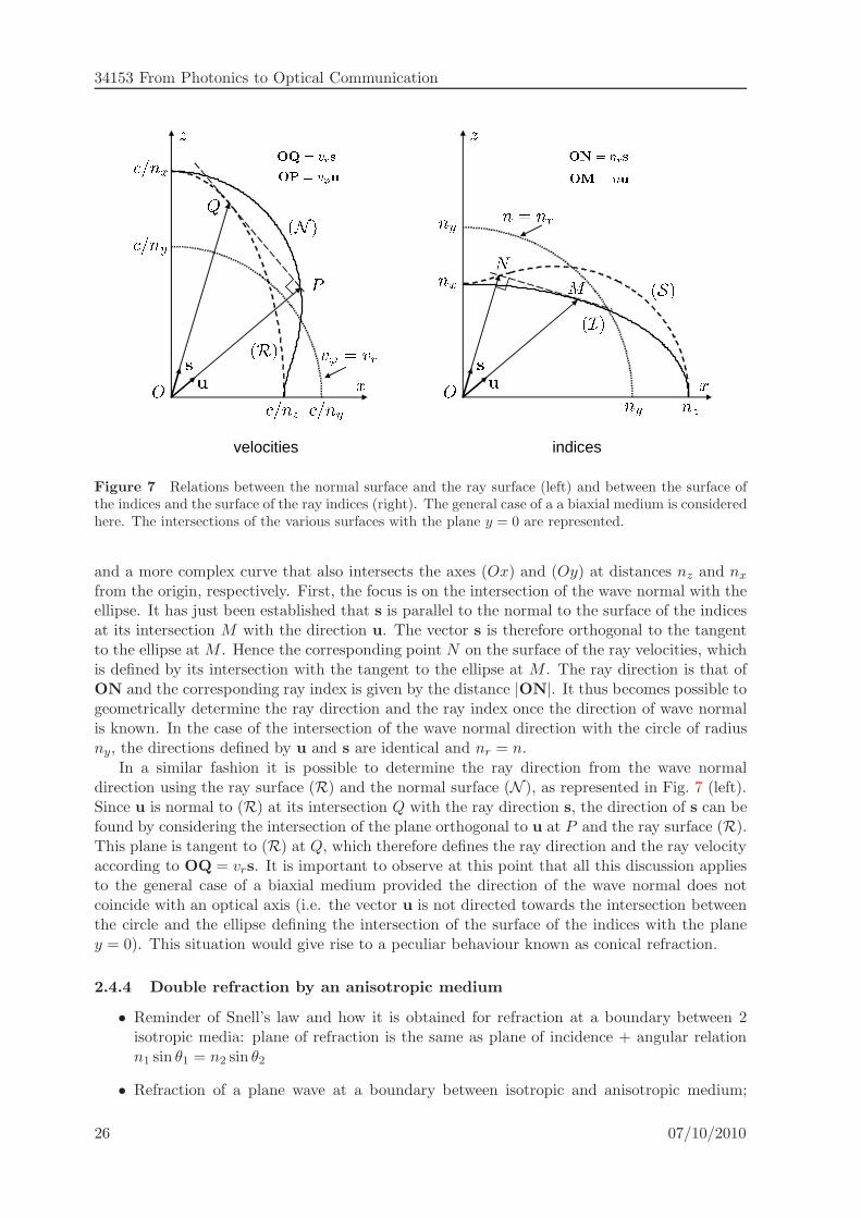
• Reminder of Snell’s law and how it is obtained for refraction at a boundary between 2isotropic media: plane of refraction is the same as plane of incidence + angular relationn1 sin θ1 = n2 sin θ2
• Refraction of a plane wave at a boundary between isotropic and anisotropic medium;
26 07/10/2010
Anisotropic Media and the Linear Electro-Optic Effect
isotropic
anisotropic
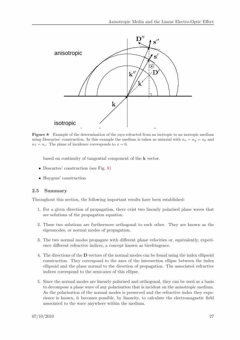
Figure 8 Example of the determination of the rays refracted from an isotropic to an isotropic mediumusing Descartes’ construction. In this example the medium is taken as uniaxial with nx = ny = n0 andnz = ne. The plane of incidence corresponds to x = 0.
based on continuity of tangential component of the k vector.
• Descartes’ construction (see Fig. 8)
• Huygens’ construction
2.5 Summary
Throughout this section, the following important results have been established:
1. For a given direction of propagation, there exist two linearly polarised plane waves thatare solutions of the propagation equation.
2. These two solutions are furthermore orthogonal to each other. They are known as theeigenmodes, or normal modes of propagation.
3. The two normal modes propagate with different phase velocities or, equivalently, experi-ence different refractive indices, a concept known as birefringence.
4. The directions of the D vectors of the normal modes can be found using the index ellipsoidconstruction. They correspond to the axes of the intersection ellipse between the indexellipsoid and the plane normal to the direction of propagation. The associated refractiveindices correspond to the semi-axes of this ellipse.
5. Since the normal modes are linearly polarised and orthogonal, they can be used as a basisto decompose a plane wave of any polarisation that is incident on the anisotropic medium.As the polarisation of the normal modes is preserved and the refractive index they expe-rience is known, it becomes possible, by linearity, to calculate the electromagnetic fieldassociated to the wave anywhere within the medium.
07/10/2010 27

34153 From Photonics to Optical Communication
3 The linear electro-optic effect
The isotropy or anisotropy of a medium can be modified under the action of external constraints.Some isotropic media can become anisotropic under these constraints, while the propertiesof some media that are already anisotropic can be modified. This induced anisotropy canarise from the application of an external electric field, an external magnetic field, or somemechanical constraints that will change the density of the material, hence its refractive index.The corresponding modification of the anisotropic properties of the medium are known aselectro-optic, magneto-optic, and photoelastic or elasto-optic effects, respectively. The acousto-
optic effect, which can be exploited to perform light modulation at relatively low speeds, isactually a photoelastic effect where the required changes of refractive index are induced byan acoustic wave propagating through the medium. In the following, the electro-optic effectwill be considered since it is commonly used to perform high speed modulation of light withbandwidths of the order of several tens of gigahertz.
It has been seen in Sect. 2.3 that the anisotropy of a medium can be characterised throughits index ellipsoid. Assuming a coordinate system that coincides with the principal axes of thedielectric tensor of the medium, the index ellipsoid can be written
x2
n2x
+y2
n2y
+z2
n2z
= 1. (160)
To simplify the notations, the equation of the index ellipsoid can also be expressed accordingto
B01x
2 +B02y
2 +B03z
2 = 1, (161)
where the superscript 0 denotes the initially unperturbed state and
B01 =
1
n2x
, B02 =
1
n2y
, B03 =
1
n2z
. (162)
Under the influence of an external applied electric field Ea, the anisotropy of the medium ismodified, resulting in a deformation of the index ellipsoid. In the most general case, the equationof the deformed index ellipsoid can be written
B1x2 +B2y
2 +B3z2 + 2B4yz + 2B5xz + 2B6xy = 1. (163)
Assuming that the variation of the Bi coefficients has a linear dependence on the appliedelectric field
B1 −B01
B2 −B02
B3 −B03
B4
B5
B6
=
r11 r12 r13r21 r22 r23r31 r32 r33r41 r42 r43r51 r52 r53r61 r62 r63
Eax
Eay
Eaz
, (164)
where [r] is known as the electro-optic tensor. This type of electro-optic effect having a lineardependence on the applied electric field is known as the Pockels effect22.
22Friedrich Carl Alwin Pockels, Vicenza, 1865 – Heidelberg 1913.
28 07/10/2010

Anisotropic Media and the Linear Electro-Optic Effect
Remark: on the notations
The relation between the change of the coefficients of the equation of the index ellipsoid andthe applied external field has been written in (164) according to
∆B = B (Ea)−B (Ea = 0) = [r]Ea. (165)
Since the Bi are the coefficients of the quadratic form associated with the ellipsoid index, theycan be identified with the coefficients of the impermeability tensor
[η] =
η11 η12 η13η21 η22 η23η31 η32 η33
. (166)
Indeed, the equation of the index ellipsoid is23
ηijxixj = 1, (167)
where Einstein’s summation rule over repeated indices has been applied.
Without any prior knowledge of the physical phenomena involved, the tensor ∆ηij has 9elements and the vector Ea has three components. Therefore the relation linking ∆ηij to Ea
should be written
∆ηij = rijkEk, (168)
where the summation over k is implicit and where rijk, which is known as a third rank tensor,should has 27 elements. However, the study of the physics of the problem leads to the conclu-sion that ∆η is symmetric and therefore has only 6 distinct elements. Consequently rijk onlypossess 18 distinct elements (this number can be reduced further by introducing more physicalconsiderations and examining the symmetries of the crystal). It then becomes possible to adoptthe so-called contracted notations for ij
11 → 1 23 → 4
22 → 2 13 → 5
33 → 3 12 → 6
resulting in
∆Bl = rlkEak, (169)
which corresponds to (164).
3.1 Determination of the refractive indices under an applied electric field
In this section, the general procedure to determine the directions of the normal modes andassociated refractive indices is illustrated on a particular example. Here the classic case of acrystal of potassium dihydrogen phosphate (KH2PO4), known in short as KDP, is considered.KDP is a uniaxial crystal whose index ellipsoid can be written in its principal axes (x,y, z)
x2
n2o
+y2
n2o
+z2
n2e
= 1, (170)
23The coefficient 2 in front of the cross products xixj where i 6= j in the equations of the index ellipsoid suchas (163) appears due to the symmetry of [η] .
07/10/2010 29

34153 From Photonics to Optical Communication
where no = 1.5074 and ne = 1.4669 at λ = 633 nm. It belongs to the 42m class for whichsymmetry considerations would enable to show that the electro-optic tensor can be expressedas
r42m =
0 0 00 0 00 0 0r41 0 00 r41 00 0 r63
. (171)
In the case of KDP, the values of the electro-optic coefficients at 633 nm are r41 = 8×10⁻¹² m/Vand r63 = 11 × 10−12 m/V. Under an applied external electric field Ea, the index ellipsoidbecomes
x2
n2o
+y2
n2o
+z2
n2e
+ 2r41Eaxyz + 2r41Eayxz + 2r63Eazxy = 1. (172)
Eq. (172) shows that the principal axes of the crystal have been rotated by applying an externalelectric field. In order to find out the new principal axes and associated refractive indices, itis necessary to diagonalise the quadratic form associated to the new index ellipsoid (172). Forsimplicity, the analysis is carried further in the case of an external electric field applied in thez direction. The index ellipsoid thus becomes
x2
n2o
+y2
n2o
+z2
n2e
+ 2r63Eazxy = 1, (173)
and the matrix of its associated quadratic form can be expressed in the basis (x,y, z) as
Q =
B1 B6 0B6 B1 00 0 B3
, (174)
where B1 = 1/n2o, B3 = 1/n2
e and B6 = r63Eaz . The eigenvalues of Q can be found by solvingthe equation ∣∣∣∣∣∣
B1 − λ B6 0B6 B1 − λ 00 0 B3 − λ
∣∣∣∣∣∣= 0, (175)
leading to
(B3 − λ)[(B1 − λ)2 −B2
6
]= 0. (176)
Hence the eigenvalues
λ1 = B1 +B6, (177)
λ2 = B1 −B6, (178)
λ3 = B3. (179)
In order to define the directions of the axes of the deformed index ellipsoid, it is necessary tofind the eigenvectors associated to the eigenvalues (177)-(179). This step is detailled below foreach of the eigenvalues.
• λ1 = B1 +B6
The eigenvectors can be found by solving the system:
30 07/10/2010

Anisotropic Media and the Linear Electro-Optic Effect
x− y = 0
(B3 −B1 −B6) z = 0(180)
Hence an eigenvector associated with the eigenvalue λ1 is x′ = 1√2(x+ y).
• λ2 = B1 −B6
The eigenvectors can be found by solving the system:
x+ y = 0
(B3 −B1 +B6) z = 0(181)
Hence an eigenvector associated with the eigenvalue λ2 is y′ = 1√2(−x+ y).
• λ3 = B3
The eigenvectors can be found by solving the system:
(B1 −B3) x + B6 y = 0B6 x + (B1 −B3) y = 0
(B3 −B3) z = 0(182)
Hence an eigenvector associated with the eigenvalue λ3 is z′ = z.
The transformation matrix from the old basis (x,y, z) to the new basis (x′,y′, z′) can be ob-tained by expressing the components of the vectors of the new basis on the old basis, leadingto
P =
1√2
− 1√2
01√2
1√2
0
0 0 1
, (183)
which corresponds to the matrix of a rotation of angle π/4 around z.In the new coordinate system, the equation of the deformed ellipsoid index is
λ1x′2 + λ2y
′2 + λ3z′2 = 1, (184)
which can also be expressed in terms of the refractive indices along the axes of the deformedellipsoid
x′2
n2x′
+y′2
n2y′
+z′2
n2z′
= 1, (185)
where n′x, n
′y and n′
z are obtained through the relations
1
n2x′
=1
n2o
+ r63Eaz (186)
1
n2y′
=1
n2o
− r63Eaz (187)
1
n2z′
=1
n2e
(188)
From (186)
nx′ =no
(1 + n2or63Eaz)
1/2≈ n0
(1− 1
2n2or63Eaz
)(189)
07/10/2010 31
34153 From Photonics to Optical Communication
π/4
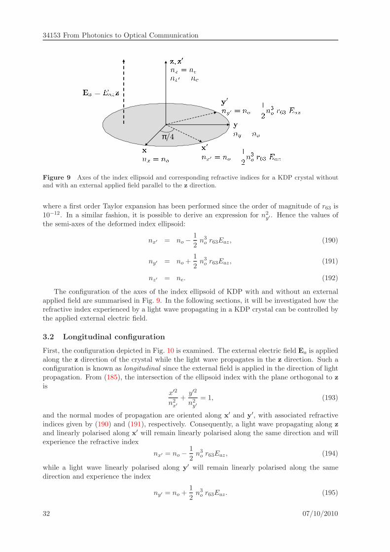
Figure 9 Axes of the index ellipsoid and corresponding refractive indices for a KDP crystal withoutand with an external applied field parallel to the z direction.
where a first order Taylor expansion has been performed since the order of magnitude of r63 is10−12. In a similar fashion, it is possible to derive an expression for n2
y′ . Hence the values ofthe semi-axes of the deformed index ellipsoid:
nx′ = no −1
2n3o r63Eaz , (190)
ny′ = no +1
2n3o r63Eaz , (191)
nz′ = ne. (192)
The configuration of the axes of the index ellipsoid of KDP with and without an externalapplied field are summarised in Fig. 9. In the following sections, it will be investigated how therefractive index experienced by a light wave propagating in a KDP crystal can be controlled bythe applied external electric field.
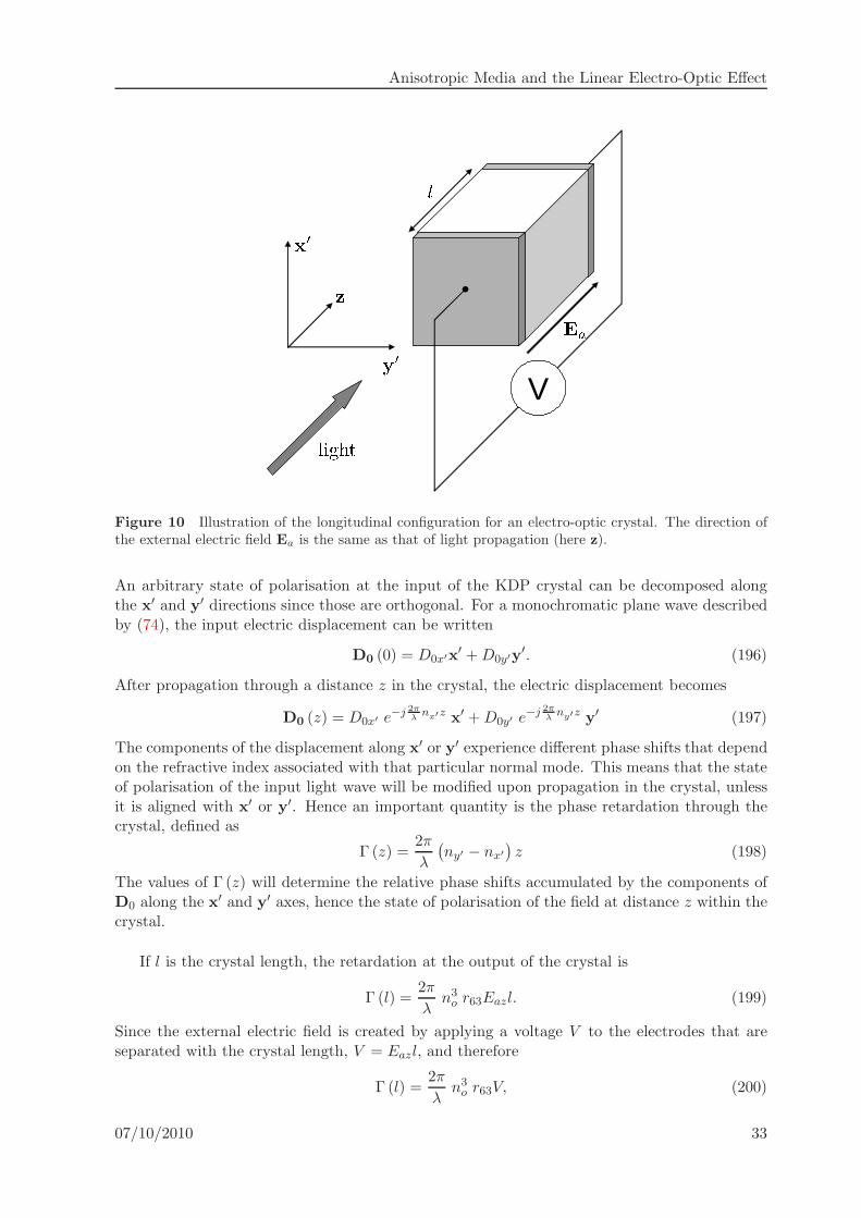
3.2 Longitudinal configuration
First, the configuration depicted in Fig. 10 is examined. The external electric field Ea is appliedalong the z direction of the crystal while the light wave propagates in the z direction. Such aconfiguration is known as longitudinal since the external field is applied in the direction of lightpropagation. From (185), the intersection of the ellipsoid index with the plane orthogonal to z
isx′2
n2x′
+y′2
n2y′
= 1, (193)
and the normal modes of propagation are oriented along x′ and y′, with associated refractiveindices given by (190) and (191), respectively. Consequently, a light wave propagating along z
and linearly polarised along x′ will remain linearly polarised along the same direction and willexperience the refractive index
nx′ = no −1
2n3o r63Eaz , (194)
while a light wave linearly polarised along y′ will remain linearly polarised along the samedirection and experience the index
ny′ = no +1
2n3o r63Eaz. (195)
32 07/10/2010
Anisotropic Media and the Linear Electro-Optic Effect
V
Figure 10 Illustration of the longitudinal configuration for an electro-optic crystal. The direction ofthe external electric field Ea is the same as that of light propagation (here z).
An arbitrary state of polarisation at the input of the KDP crystal can be decomposed alongthe x′ and y′ directions since those are orthogonal. For a monochromatic plane wave describedby (74), the input electric displacement can be written
D0 (0) = D0x′x′ +D0y′y′. (196)
After propagation through a distance z in the crystal, the electric displacement becomes
D0 (z) = D0x′ e−j 2πλnx′z x′ +D0y′ e
−j 2πλny′z y′ (197)
The components of the displacement along x′ or y′ experience different phase shifts that dependon the refractive index associated with that particular normal mode. This means that the stateof polarisation of the input light wave will be modified upon propagation in the crystal, unlessit is aligned with x′ or y′. Hence an important quantity is the phase retardation through thecrystal, defined as
Γ (z) =2π
λ
(ny′ − nx′
)z (198)
The values of Γ (z) will determine the relative phase shifts accumulated by the components ofD0 along the x′ and y′ axes, hence the state of polarisation of the field at distance z within thecrystal.
If l is the crystal length, the retardation at the output of the crystal is
Γ (l) =2π
λn3o r63Eazl. (199)
Since the external electric field is created by applying a voltage V to the electrodes that areseparated with the crystal length, V = Eazl, and therefore
Γ (l) =2π
λn3o r63V, (200)
07/10/2010 33

34153 From Photonics to Optical Communication
V
Figure 11 Transverse configuration for an electro-optic crystal. The external electric field Ea is appliedorthogonally to the direction of light propagation.
which is customarily expressed as
Γ = πV
Vπ, (201)
where the quantity
Vπ =λ
2n3o r63
(202)
is known as the half wave voltage of the crystal under longitudinal configuration. Applying avoltage equal to Vπ to the electrodes induces an electro-optic retardation of π, or equivalentlycreates an optical path length difference of λ/2 between the two normal modes. It is importantto notice that, under longitudinal configuration, Vπ only depends on the material parametersno and r63. At 633 nm, the half-wave voltage is therefore equal to Vπ = 8400 V. This voltageis independent of the geometry of the crystal.
Since in this configuration the direction of the applied electric field is the same as thatof light propagation, it should be ensured that the electrodes that are employed to apply thevoltage that induces Ea are transparent to the optical wave.
3.3 Transverse configuration
In the so-called transverse configuration the direction of light propagation is orthogonal to thedirection of the applied electric field. Fig. 11 illustrates such a configuration where Ea is appliedalong z and the wave propagates in the y′ direction. In this case, waves linearly polarised alongx′ or z will remain linearly polarised along the same directions and will experience refractiveindices equal to
nx′ = no −1
2n3o r63Eaz, (203)
andnz = ne, (204)
respectively. Hence the electro-optic retardation at the crystal output
Γ(l) =2π
λ(nz − nx′) l =
2π
λ(ne − n0) l +
πn3o r63Eaz l
λ(205)
34 07/10/2010

Anisotropic Media and the Linear Electro-Optic Effect
The first term corresponds to a fixed retardation induced by the birefringence of the crystal.It could in principle be compensated by a proper choice of the crystal length so that thefixed retardation is an integer multiple of 2π at the wavelength of interest, or by inserting anappropriate wave plate. In practice, the temperature dependence of the static birefringencene − n0 might make such a compensation challenging. This term will nevertheless be ignoredin the discussion that follows where the focus is on the induced birefringence.
In the transverse configuration, the external electric field is induced by a voltage appliedacross the crystal whose thickness is e, hence V = Eaze, and the induced retardation becomes
Γ =πn3
o r63V
λ
(l
e
). (206)
Similarly to the longitudinal case, it is possible to define a half-wave voltage
Vπ =λ
n3o r63
(el
), (207)
so that the induced retardation can be expressed according to (201). It is however important tonote that, contrarily to the longitudinal case, both the induced retardation and the half-wavevoltage depend on the form factor e/l. It is therefore possible to reduce Vπ (i.e. the voltagenecessary to induce a retardation equal to π) by increasing the interaction length l between theapplied electric field and the optical wave, or by reducing the electrode spacing e. For opticalcommunication applications, guided wave structures will be used to modify the properties of alight wave through the electro-optic effect. Therefore the required waveguide geometry will seta lower limit to e. Consequently, the product Vπl can be used as a figure of merit for transverseelectro-optic modulators. Furthermore, since the external electric field is applied orthogonallyto the direction of light propagation, no difficulty arises due to the electrode configuration withrespect to the optical path, as is the case for the longitudinal configuration.
Consequently the transverse configuration will be preferred for the practical application ofthe electro-optic effect to the modulation of light, as described in more details in the followingsection.
4 Electro-optic modulation
4.1 The electro-optic effect in lithium-niobate
Lithium niobate (LiNbO3) is the material customarily used for light modulation in opticalcommunication applications due to its relatively large electro-optic coefficient and the goodcontrol of the technology required to produce low loss optical modulators. LiNbO3 is a uniaxialcrystal whose unperturbed index ellipsoid is given, in the principal axes system, by
x2
n2o
+y2
n2o
+z2
n2e
= 1, (208)
where commonly reported values at 633 nm for the ordinary and extraordinary refractive indicesare n0 = 2.29 and ne = 2.2, respectively. It belongs to the 3m crystal point group and itsdielectric tensor is therefore given by
r3m =
0 −r22 r130 r22 r130 0 r330 r51 0r51 0 0−r22 0 0
. (209)
07/10/2010 35

34153 From Photonics to Optical Communication
x-cut z-cut
Figure 12 Possible configurations for efficient electro-optic modulation using lithium niobate. Theexternal field is applied along the z direction while the light propagates along the longest dimension ofthe crystal.
Typical values for the electro-optic coefficients are24:
r22 = 3.4 pm/V, r13 = 8.6 pm/V,
r51 = 28.0 pm/V, r33 = 30.8 pm/V.
Strictly speaking, those values apply at a wavelength of 633 nm25. Even though those coefficientsare known to be wavelength dependent, and in the absence of readily available data at thetelecommunication wavelength of 1550 nm, these values will be used in the present discussionof LiNbO3 modulators. More data on the physical properties of lithium niobate, including acomparison of values for the refractive indices and electro-optic coefficients reported by variousauthors, can be found in published reviews such as [8].
In any case, r33 is the largest coefficient of the electro-optic tensor. For practical modulationapplications, it is desirable to induce the largest possible refractive index change for a givenapplied voltage. In order to exploit r33, the external modulating electric fieldEa should thereforebe aligned with the z direction: Ea = Eazz. Under those conditions, the index ellipsoid becomes
(1
n2o
+ r13Eaz
)x2 +
(1
n2o
+ r13Eaz
)y2 +
(1
n2e
+ r33Eaz
)z2 = 1. (210)
One important observation is that the principal axes of the index ellipsoid of LiNbO3 aretherefore unchanged when an electric field parallel to z is applied to the crystal.
For practical modulation applications the following external requirements should be satisfied:
1. The applied electric field should be parallel to the z direction in order to exploit the larger33 electro-optic coefficient.
2. The modulation should be transverse in order to benefit from the form factor e/l discussedin Sec. 3.3.
Those requirements lead to the three possible configurations depicted in Fig. 12. In thoseconfigurations, the light propagates along the longest dimension of the crystal in order tobenefit from the form factor. They are customarily referred to as x-cut and z-cut. In thex-cut configuration, the plane from which the waveguide will be implanted and on which theelectrodes will be deposited is perpendicular to the x crystal direction.
24Those values result from high frequency (50–86 MHz) measurements performed at 633 nm and first reportedin [7]. Slightly different values can be found in the literature, depending on the measurement conditions andexperimental method. Nevertheless the values presented here will be considered sufficiently accurate for thepurpose of this note.
25The justification for this wavelength is that it corresponds to the line of helium-neon lasers.
36 07/10/2010

Anisotropic Media and the Linear Electro-Optic Effect
4.1.1 x-cut configuration
For transverse modulation, the light has to propagate along the y direction. The refractiveindex along z is therefore given by
1
n′2z
=1
n2e
+ r33Eaz =1
n2e
(1 + r33n
2eEaz
), (211)
hence, with the usual assumption that r33n2eEaz ≪ 1,
n′z = ne −
1
2n3e r33Eaz . (212)
Similarly, the refractive index in the x direction can be shown to be
n′x = no −
1
2n3o r13Eaz . (213)
Since the phase shift experienced by a light wave propagating into a length l of a mediumof refractive index n is equal to φ = 2π
λ nl, it is clear that for efficient phase modulation thelight wave should be polarised along the z direction. Consequently, in the x-cut configuration,efficient phase modulation is performed for the transverse electric (TE) mode.
4.1.2 z-cut configuration
In the z-cut configurations, the top plane of the crystal is orthogonal to the z direction, asillustrated in Fig. 12. Two possibilities exist for the direction of light propagation: either alongx or along y. In the case of propagation along x, the principal refractive indices under anapplied electric field along z are
n′y = no −
1
2n3o r13Eaz , (214)
n′z = ne −
1
2n3e r33Eaz, (215)
while if propagation takes place in the y direction, the indices
n′x = no −
1
2n3o r13Eaz , (216)
n′z = ne −
1
2n3e r33Eaz, (217)
should be considered. In both cases, it can be seen that efficient phase modulation takes placewhen the electric field of the light wave is polarised along the z direction, which corresponds tothe transverse magnetic (TM) mode of the waveguide.
Fig. 13 shows cross sections of practical structures used for electro-optic modulation inLiNbO3. The light is confined to a waveguide that is realised by locally raising the refractiveindex of the lithium niobate substrate. This is usually achieved by selectively diffusing titaniuminto the crystal. Photolithographic techniques are used to depose a Ti film whose width andlength are similar to those of the final waveguide on top of the crystal. The sample is thenheated around 1000C for several hours, which allows the titanium to diffuse into the crystaland raises its refractive index. This process results in waveguides where the relative refractiveindex difference between the core and the cladding is of the order of ∆ ∼ 0.5–1% and the lossis less than 0.2 dB/cm. A buffer layer made of silica (SiO2) is then deposited on top of thecrystal. This layer prevents the optical field from extending into the metal electrodes, which
07/10/2010 37
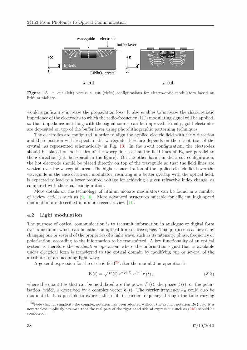
34153 From Photonics to Optical Communication
electrodewaveguide
LiNbO3 crystal
buffer layer
Ea field
x-cut z-cut
Figure 13 x−cut (left) versus z−cut (right) configurations for electro-optic modulators based onlithium niobate.
would significantly increase the propagation loss. It also enables to increase the characteristicimpedance of the electrodes to which the radio-frequency (RF) modulating signal will be applied,so that impedance matching with the signal source can be improved. Finally, gold electrodesare deposited on top of the buffer layer using photolithographic patterning techniques.
The electrodes are configured in order to align the applied electric field with the z directionand their position with respect to the waveguide therefore depends on the orientation of thecrystal, as represented schematically in Fig. 13. In the x-cut configuration, the electrodesshould be placed on both sides of the waveguide so that the field lines of Ea are parallel tothe z direction (i.e. horizontal in the figure). On the other hand, in the z-cut configuration,the hot electrode should be placed directly on top of the waveguide so that the field lines arevertical over the waveguide area. The higher concentration of the applied electric field over thewaveguide in the case of a z-cut modulator, resulting in a better overlap with the optical field,is expected to lead to a lower required voltage for achieving a given refractive index change, ascompared with the x-cut configuration.
More details on the technology of lithium niobate modulators can be found in a numberof review articles such as [9, 10]. More advanced structures suitable for efficient high speedmodulation are described in a more recent review [11].
4.2 Light modulation
The purpose of optical communication is to transmit information in analogue or digital formover a medium, which can be either an optical fibre or free space. This purpose is achieved bychanging one or several of the properties of a light wave, such as its intensity, phase, frequency orpolarisation, according to the information to be transmitted. A key functionality of an opticalsystem is therefore the modulation operation, where the information signal that is availableunder electrical form is transferred to the optical domain by modifying one or several of theattributes of an incoming light wave.
A general expression for the electric field26 after the modulation operation is
E (t) =√
P (t) e−jφ(t) ejω0t e (t) , (218)
where the quantities that can be modulated are the power P (t), the phase φ (t), or the polar-isation, which is described by a complex vector e (t). The carrier frequency ω0 could also bemodulated. It is possible to express this shift in carrier frequency through the time varying
26Note that for simplicity the complex notation has been adopted without the explicit notation Re . . .. It isnevertheless implicitly assumed that the real part of the right hand side of expressions such as (218) should beconsidered.
38 07/10/2010

Anisotropic Media and the Linear Electro-Optic Effect
Figure 14 Principle of an electro-optic phase modulator illustrated here for a z-cut LiNbO3 crystal.
phase term φ (t), according to
ω (t) = ω0 −∂φ
∂t(t) , (219)
where ω (t) is the instantaneous frequency.
It has been seen in the previous sections how the refractive index experienced by a lightwave can be changed by applying an external field to an electro-optic material. This refractiveindex change has been shown to depend on the orientation of the applied external field withrespect to the principal axes of the crystal, as well as on the polarisation of the optical field.In the following, it will be shown how this property can be exploited to modulated the phase,polarisation or intensity of a light wave.
4.3 Phase modulation
The application of the electro-optic effect to phase modulation is straightforward, as representedin Fig. 14 for a z-cut LiNbO3 crystal. If the incoming light is linearly polarised along thez direction, which is one of the two eigenpolarisations of the crystal, it will remain linearlypolarised along the same direction over propagation through the crystal and will experience thephase shift
φ =2π
λn′z l, (220)
where l is the crystal length and n′z is given by (217). The alignment of the input state
of polarisation with the direction z can be ensured by using a polarisation controller, or byplacing a polariser parallel to z in front of the crystal, as represented in Fig. 14. Since n′
z
depends on the external electric field, which is itself created by a time varying voltage V (t)applied across the crystal, the phase of the light wave will be modulated according to V (t) afterit has propagated through the crystal. Neglecting a constant phase shift, and since V = −Eae,where e is the crystal thickness, the electro-optically induced phase variation can be written
φ (t) = πV (t)
Vπ, (221)
where the half-wave voltage for the present configuration depends on the electro-optic coefficientaccording to
Vπ =λ
n3e r33
(el
). (222)
Note that (222) assumes a uniform distribution of the electric field over the waveguideand moreover does not take into account the transverse distribution of the optical mode in
07/10/2010 39

34153 From Photonics to Optical Communication
Figure 15 Principle of an electro-optic polarisation modulator.
the waveguide. In practice, one should calculate the overlap integral between the optical andapplied electric fields [12, 13]
γ =e
V
∫∫E2 (x, z)Ea (x, z) dx dz∫∫
E2 (x, z) dx dz, (223)
so that
Vπ =λ
n3e r33γ
(el
). (224)
Assuming e = 8 µm and γ = 0.5, and using the values ne = 2.14 and r33 = 30.8 pm/V, leads toa figure of merit of Vπ l = 8.2 V · cm for a z-cut LiNbO3 modulator at 1550 nm. In practice onewould like to operate the modulator with as low a voltage as possible by increasing the devicelength. However, it will be shown in Sec. 5 that some trade-offs between voltage requirementand device length need to be found for high-frequency modulation applications.
4.4 Polarisation modulation
As discussed in Sec. 3.2, the state of polarisation of an optical field which is not linearly polarisedalong one of the principal axes can be controlled by applying an external electric field to anelectro-optic crystal. For illustration, the case of a z-cut LiNbO3 crystal is considered in theconfiguration represented in Fig. 15. The incoming light wave is linearly polarised at an angleof 45 with the directions x and z, so that its displacement vector can be expressed as
D0 (0) = D0 i, (225)
where i = 1√2(x+ z) corresponds to its direction of polarisation. At the output of the crystal,
the field can be written
D0 (l) =D0√2e−j 2π
λn′
zl z+D0√2e−j 2π
λn′
xl x, (226)
or equivalently
D0 (l) =D0√2
(e−j Γ
2 z+ ejΓ2 x)e−j π
λ(n′
z+n′
x), (227)
where the retardation Γ is
Γ =2π
λ
(n′z − n′
x
)l. (228)
40 07/10/2010

Anisotropic Media and the Linear Electro-Optic Effect
Eq. (227) enables to directly express the field at the output of the crystal by mean of its Jonesvector, expressed in the (z,x) basis according to
J(z,x) (l) =1√2
(e−j Γ
2
ejΓ2
), (229)
from which its state of polarisation can be determined, depending on the value of Γ. Using(216) and (217), the retardation can be expanded into
Γ =2π
λ(ne − no) l +
π
λ
(n3e r33 − n3
o r13)( l
e
)V, (230)
where the external field across the crystal has been related to the applied voltage according toV = −Eaze. As in the case of KDP studied in Sec. 3.3, the retardation consists of two terms.The first term is a static term, Γ0, that results from the natural birefringence of the crystal27.The second term corresponds to the electro-optically induced birefringence and can be writtenunder the usual form Γeo = πV/Vπ, where the half-wave voltage is equal to
Vπ =λ
n3e r33 − n3
o r13
(el
). (231)
Eq. (230) shows that the natural birefringence can be compensated in practice by adding aconstant d.c. bias to the modulating voltage. If the voltage applied to the crystal is expressedas V = V0 + Vs, where V0 is a d.c. offset and Vs is the modulating signal, the condition forcompensation of the natural birefringence can be expressed as Γ0 + πV0/Vπ = k2π. When sucha condition is satisfied, the state of polarisation of the incoming beam is not modified whenVs = 0 V. On the other hand, if a modulating voltage equal to Vs = Vπ is applied to the crystal,Γeo = π, and the displacement at the output of the crystal becomes
D0 (l) =D0√2(x− z) e−j π
λ(n′
z+n′
x) ejπ2 , (232)
so that the polarisation of the light wave at the output of the crystal is linear and parallel toj = 1√
2(x− z), which is a vector orthogonal to i. It is convenient to express the output field in
the general case in the basis (i, j). Starting from (227), one immediately obtains
D0 (l) = D0
(cos
Γ
2i+ j sin
Γ
2j
)e−j π
λ(n′
z+n′
x), (233)
Consequently, provided the static birefringence has been adequately compensated:
• if Vs = 0 V, the state of polarisation of the light at the output of the crystal is the sameas the one at the input, i.e. linear and parallel to i.
• if Vs = Vπ, the state of polarisation of the light at the output of the crystal is linear andorthogonal to i
Polarisation modulation between two orthogonal linear states parallel to i and j, respectively,has therefore been achieved from a binary electrical signal taking the values 0, Vπ. In thecontext of optical communications, such a modulation is known as polarisation shift keying
(PolSK).
27This term could in principle be compensated by properly adjusting the length of the crystal so that the staticretardation is made equal to k2π, where k is an integer. However, this would require a precision of the order ofthe wavelength for the cleaving of the crystal.
07/10/2010 41

34153 From Photonics to Optical Communication
In the basis (i, j), the Jones vector at the output of the crystal can be written
J(i, j) (l) =
(cos Γ
2
j sin Γ2
), (234)
which corresponds to the expression of a general elliptical state of polarisation having an el-lipticity Γ/2 expressed in the coordinate system that corresponds to the axes of the ellipse.Therefore, depending on the value of the applied voltage, hence Γ, all elliptical states of polari-sation with axes i, j can be obtained at the output of the crystal starting from an input that islinearly polarised along i.
4.5 Intensity modulation
So far it has been shown how the linear electro-optic effect can be used to modify the refractiveindex of a crystal according to an applied electric field. This property can be used in a straight-forward way to realise a phase modulator. Utilising the induced birefringence of an electro-opticcrystal can also lead to polarisation modulation. However, optical communication systems re-lying on either phase or polarisation modulation are difficult to implement in practice. At thereceiver side, the most straightforward detection scheme, known as direct detection, consists of aphotodiode that only responds to the power of the light that is incident upon it. A photodiodeproduces a current whose intensity i is proportional to the received optical power P accordingto i (t) = RP (t), where R is known as the responsivity of the photodiode. Consequently, allinformation contained in the phase or the polarisation of the incoming light wave is lost in sucha detection process. The phase information can nevertheless be recovered by using a coherent
detection scheme where the incoming optical signal beats with light emitted by a local oscillatorlaser located at the receiver. Such schemes have been the object of intense investigations inthe late 80’s and early 90’s. They are however difficult to implement in practice, in part dueto stability requirements and polarisation sensitivity. Nevertheless, thanks to the significantprogress accomplished over the past decade, a revival of such techniques is currently observedin a number of research laboratories worldwide. It will be seen later in this course28 how thedifficulty inherent to phase detection can be overcome by converting first the phase modulatedsignal into an intensity modulated signal, followed by direct detection.
Polarisation detection also requires some complex receiver structures, or the use of a po-larisation discriminating element, such as a polariser, followed by direct detection. However,polarisation effects in optical fibres also make such schemes difficult to implement in practice.
Consequently, the modulation of the intensity of a light wave, in conjunction with directdetection, is so far the preferred method for transmitting information in optical communicationsystems. Since the electro-optic effect only affects the phase of the signal, some techniquesneed to be found to achieve intensity modulation. This can be performed by converting eitherpolarisation modulation or phase modulation into intensity modulation.
4.5.1 Polarisation modulator followed by a polariser
The first scheme, represented in Fig. 16, simply consists of the polarisation modulator structurestudied in Sec. 4.3, followed by a polariser aligned with the j direction. When no modulatingvoltage is applied to the crystal, and provided its natural birefringence is properly compensated,the state of polarisation of the light at the output of the crystal is parallel to i, hence orthogonalto j, and no light is transmitted by the polariser. On the other hand, when a modulating voltageequal to Vπ is applied, the output state of polarisation becomes parallel to j and the integrality
28See section on “Phase modulation”.
42 07/10/2010
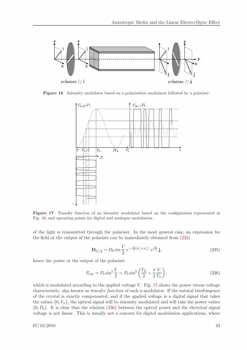
Anisotropic Media and the Linear Electro-Optic Effect
Figure 16 Intensity modulator based on a polarisation modulator followed by a polariser.
Figure 17 Transfer function of an intensity modulator based on the configuration represented inFig. 16, and operating points for digital and analogue modulation.
of the light is transmitted through the polariser. In the most general case, an expression forthe field at the output of the polariser can be immediately obtained from (233)
D0//j = D0 sinΓ
2e−j π
λ(n′
z+n′
x) ejπ2 j, (235)
hence the power at the output of the polariser
Pout = P0 sin2 Γ
2= P0 sin
2
(Γ0
2+
π
2
V
Vπ
), (236)
which is modulated according to the applied voltage V . Fig. 17 shows the power versus voltagecharacteristic, also known as transfer function of such a modulator. If the natural birefringenceof the crystal is exactly compensated, and if the applied voltage is a digital signal that takesthe values 0, Vπ, the optical signal will be intensity modulated and will take the power values0, P0. It is clear that the relation (236) between the optical power and the electrical signalvoltage is not linear. This is usually not a concern for digital modulation applications, where
07/10/2010 43

34153 From Photonics to Optical Communication
Figure 18 Principle of an intensity modulator based on a phase modulator inserted into one of thearms of a Mach-Zehnder interferometer.
the modulator will be operated between a minimum and a maximum of its transfer function,but might however be a concern for analogue applications, since it will result in the creationof undesired harmonics. In this case, one can exploit the portion of the transfer functioncurve that can approximately be considered as linear by operating the modulator around abiasing point equal to Vπ/2, also known as quadrature point, and by reducing the peak-to-peakmodulation voltage so that the linear approximation remains valid. Since an applied voltage ofVπ/2 corresponds to a retardation of π/2, adding a quarter wave plate whose axes are alignedto x and y, which is known as optical biasing, is equivalent to applying a suitable electricalbias.
4.5.2 Interferometric structure
It is well known that the light intensity at the output of a two-beam interferometer dependson the relative phase shifts experienced by the two beams after they have been separated froma common primary beam. If those phases shifts are equal (modulo 2π), then constructiveinterference occurs when the two beams are recombined. Out-of-phase beams will then resultin destructive interference. The electro-optic effect enables to control the refractive index of acrystal by an external applied electric field. A change in refractive index results in a changeof the phase shift experienced by a light beam propagating through the crystal, a principlethat has been used to design a phase modulator in Sec. 4.3. It is therefore natural to use aninterferometric structure to convert the electro-optically induced refractive index change into amodulation of the intensity of the incoming light beam.
A Mach29-Zehnder30 interferometer structure such as the one represented in Fig. 18 is cus-tomarily used for this purpose. The primary beam E0 is spatially separated by a semi-reflectingsurface. The two beams experience different paths before being recombined at another semi-reflecting surface. One of the beams will propagate through an electro-optic crystal in a phase-modulator configuration such as the one represented in Fig. 14. If E1 and E2 denote the complexenvelopes31 of the electric fields of the two beams after the semi-reflecting surface where theyrecombine, and assuming the fields have identical polarisation, the total envelope can be written
E (t) = E1 (t) + E2 (t) , (237)
29Ludwig Mach (son of Ernst Mach, Chirlitz-Turas, now Chrlice-Turany, 1838 – Vatterstetten, 1916.)30Ludwig Zehnder, 1854 – 1949.31The complex envelope of a field E (t) = E0 (t) e
−jφ(t) ejω0t e is defined as the quantity E (t) = E0 (t) e−jφ(t).
44 07/10/2010
Anisotropic Media and the Linear Electro-Optic Effect
which can be expanded into
E (t) = E01 e−jφ1 + E02 e
−jφ2(t), (238)
where φ1 and φ2 (t) are the phase shifts experienced by the upper and lower beams, respec-tively. The amplitudes E01 and E02 can be related to the amplitude E0 of the incoming beamonce the loss and reflection coefficients of the various surfaces involved for the separation andrecombination of the beams are known. Hence the power at the output of the interferometer
Pout (t) = |E (t)|2 = P1 + P2 + 2√
P1P2 cos [φ1 − φ2 (t)] , (239)
where P1 = E201 and P2 = E2
02. The output power therefore depends on the relative phase shiftexperienced by the two beams. This phase shift depends itself on the path length difference,reflections on the mirrors, as well as on the electro-optically induced refractive index changein the crystal. Assuming the constant phase shifts can be compensated, either by properdelay adjustment of by the use of compensators, the phase difference experienced by the twobeams simply depends on the electro-optic effect through φ2 (t) − φ1 = πV (t) /Vπ, where Vπ
is the half-wave voltage corresponding to the electro-optic configuration employed in the phasemodulator. If furthermore the power of the two beams can be made equal when they recombine,i.e. P0 = P1 = P2, then the power at the output of the interferometer becomes
Pout (t) = P0 cos2
(πV (t)
Vπ
), (240)
which is similar to the expression obtained in (236) for the intensity modulator structure basedon a polarisation modulator followed by a polariser. Consequently, the same issues regardingthe linearity of the modulator will be raised when such an interferometric structure is used. Inpractice, Mach-Zehnder modulators are employed to perform intensity modulation of light foroptical communication applications. Those devices are based on the Mach-Zehnder interferom-eter principle outlined here. They are however integrated on a lithium-niobate crystal substratewhere the interferometer structure is made of waveguides and Y-junctions, hence enabling therealisation of relatively compact and stable devices. This type of modulators, as well as theiruse for the generation of various modulation formats in optical communication systems, will bedescribed in detail in a separate section32.
5 High frequency electro-optic modulation
So far it has been assumed that the physical mechanisms leading to the electro-optic effectis instantaneous and that no bandwidth limitation arises from the application of the electricfield. Currently, digital optical communication systems operate typically at 10 Gbit/s and nextgeneration 40 Gbit/s systems are expected to be deployed soon. Future 100 Gbit/s solutionsare also being investigated. At all those bit rates, the first approximation is fully justified.However, the electrodes that are used to apply the modulation voltage across the electro-opticcrystal nevertheless limit the bandwidth of electro-optic modulators. The possible origin ofsuch bandwidth limitations is discussed in this section.
A first obvious limitation results from the basic structure of electro-optic modulators consid-ered so far. As illustrated for instance in Fig. 11, such a modulator consists of an electro-opticcrystal, which exhibits insulating properties, sandwiched between two electrodes. Consequentlyit is essentially a parallel plate capacitor whose capacitance depends on the dielectric constant
32See section on “The Mach-Zehnder modulator”.
07/10/2010 45

34153 From Photonics to Optical Communication
of the electro-optic material ǫ, as well as on the surface and separation of the electrodes, Aand e, respectively, according to C = ǫA/e. In order to match the impedance of the electrodesto that of the source and the transmission line that will provide the modulating signal, a loadresistance RL is used to connect the two electrodes. Consequently, seen from the source, themodulator is an RC circuit whose 3 dB bandwidth is therefore equal to
f3 dB =1
2πRLC. (241)
Therefore the capacitance of the modulator sets an upper limit to the frequency range at whichit can be operated. It has been seen in Sec. 3.3 that one of the benefits of the transverse config-uration for electro-optic modulators is that it is possible to reduce the voltage requirements inorder to achieve a given phase retardation by increasing the electrodes length l. Increasing l willalso increase the capacitance C, hence decrease the modulator bandwidth. The RC limitationdescribed above is however only valid for relatively low modulation frequencies, when the valueof the modulating signal can be considered constant over the duration of the propagation ofthe phase front through the crystal. At higher modulation frequencies, transit time effects willlimit the modulator bandwidth.
5.1 Transit time limitation
In the case of a longitudinal configuration, it has been shown in Sec.3.2 that the electro-opticretardation induced by a crystal could be expressed as (199)
Γ =π
VπEazl. (242)
Eq. (242) assumes that the applied electric field Ea is uniform over the z direction in the crystal.If this is not the case, it is necessary to consider elementary retardations
dΓ =π
VπEaz (z) dz, (243)
and integrate over the crystal length, hence
Γ =π
Vπ
∫ l
0Eaz (z) dz. (244)
For a transverse configuration, the induced retardation can be expressed according to (205) bya relation of the type
Γ =πn3
or63Eaz l
λ. (245)
Hence, if the value of the applied field is not uniform along the direction of propagation y′, theelementary retardation is
dΓ =πn3
or63Eaz (y′) dy′
λ. (246)
In both longitudinal and transverse cases, it can be seen that the electro-optic retardationinduced by an electric field whose value depends on the position along the direction of lightpropagation in the crystal can be written
Γ = a
∫ l
0Ea (ζ) dζ (247)
where a is a proportionality factor that depends on the configuration, and ζ is the positionalong the longitudinal dimension of the crystal.
46 07/10/2010
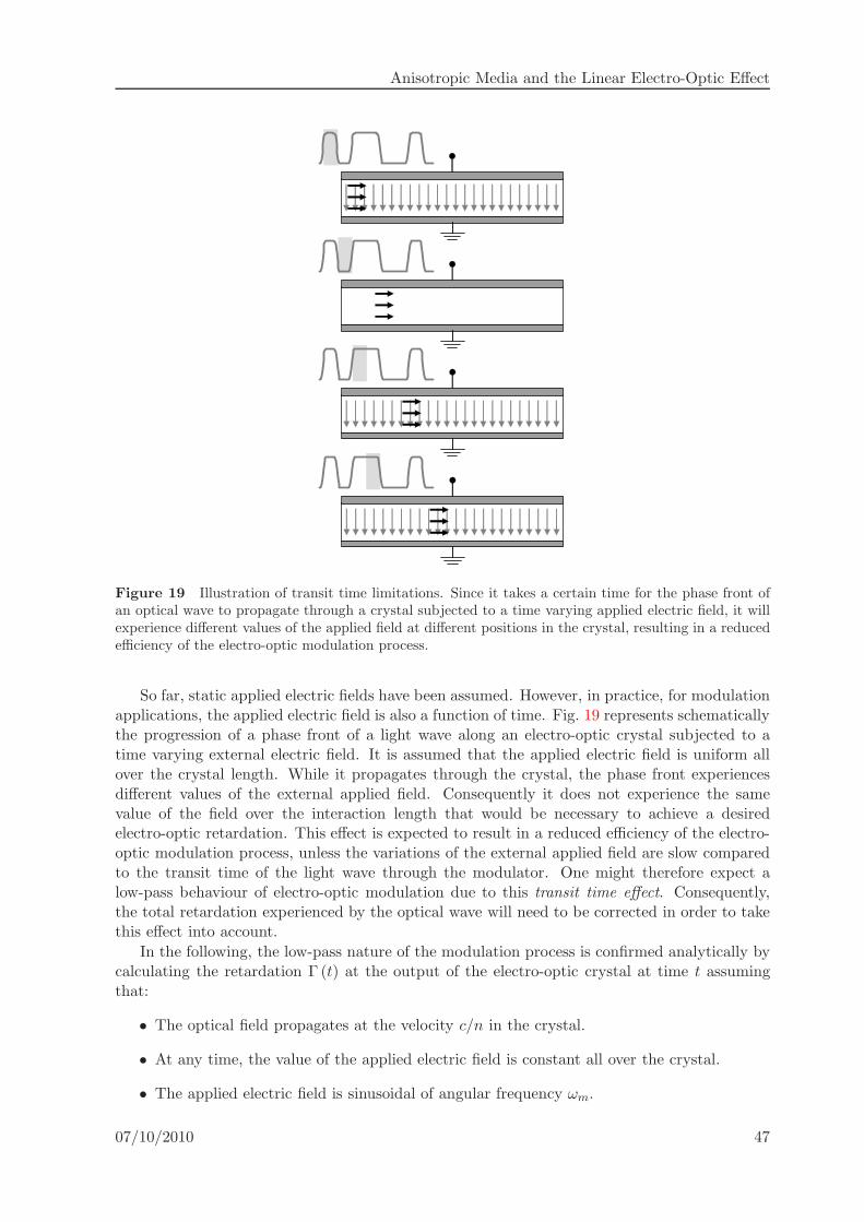
Anisotropic Media and the Linear Electro-Optic Effect
Figure 19 Illustration of transit time limitations. Since it takes a certain time for the phase front ofan optical wave to propagate through a crystal subjected to a time varying applied electric field, it willexperience different values of the applied field at different positions in the crystal, resulting in a reducedefficiency of the electro-optic modulation process.
So far, static applied electric fields have been assumed. However, in practice, for modulationapplications, the applied electric field is also a function of time. Fig. 19 represents schematicallythe progression of a phase front of a light wave along an electro-optic crystal subjected to atime varying external electric field. It is assumed that the applied electric field is uniform allover the crystal length. While it propagates through the crystal, the phase front experiencesdifferent values of the external applied field. Consequently it does not experience the samevalue of the field over the interaction length that would be necessary to achieve a desiredelectro-optic retardation. This effect is expected to result in a reduced efficiency of the electro-optic modulation process, unless the variations of the external applied field are slow comparedto the transit time of the light wave through the modulator. One might therefore expect alow-pass behaviour of electro-optic modulation due to this transit time effect. Consequently,the total retardation experienced by the optical wave will need to be corrected in order to takethis effect into account.
In the following, the low-pass nature of the modulation process is confirmed analytically bycalculating the retardation Γ (t) at the output of the electro-optic crystal at time t assumingthat:
• The optical field propagates at the velocity c/n in the crystal.
• At any time, the value of the applied electric field is constant all over the crystal.
• The applied electric field is sinusoidal of angular frequency ωm.
07/10/2010 47

34153 From Photonics to Optical Communication
time
distance
Figure 20 Notations employed for the calculation of the electro-optic retardation induced by a timevarying external electric field. The modulating field is assumed to be constant all over the crystal at anygiven time.
The notations used in the present derivation are introduced in Fig. 20. The transit time τthrough the crystal is equal to
τ =nl
c. (248)
The phase front that exits the crystal at time t was passing the position ζ in the crystal attime tζ . As it is assumed that, at any given time, the modulating field Ea (ζ, t) is constantthroughout the crystal, its value when the phase front was passing ζ was Ea (ζ, tζ) = Ea (tζ).The contribution to the total retardation of the slice of thickness dζ positioned at distance ζ inthe crystal is therefore
dΓ = a Ea (tζ) dζ. (249)
Sinceζ =
c
n(tζ − t+ τ) , (250)
the elementary retardation becomes
dΓ = a Ea (tζ)c
ndtζ , (251)
which can be integrated over the crystal length to provide the total retardation
Γ (t) =ac
n
∫ t
t−τEa (tζ) dtζ . (252)
Assuming a sinusoidal modulation,
Ea (tζ) = E0 cos (ωmtζ + ϕ) , (253)
it is convenient to introduce the complex notation
Ea (tζ) = ReE0 ejωmtζ ejϕ
(254)
in order to evaluate the integral (252), Hence
Γ (t) = Re
ac
nE0 ejϕ
∫ τ
t−τejωmtζ dtζ
, (255)
which can be easily evaluated, leading to
Γ (t) = Γ0
[sin(ωm
τ2
)
ωmτ2
]cos(ωmt− ωm
τ
2+ ϕ
)(256)
48 07/10/2010

Anisotropic Media and the Linear Electro-Optic Effect
0.0
0.2
0.4
0.6
0.8
1.0
0 3π2π
|sin
(ωmτ /
2 )
| / |ω
mτ /
2 |
ωm
τ / 2π
Figure 21 Reduction of the peak electro-optic retardation induced by transit time limitations: ωm isthe modulating signal angular frequency and τ is the transit time through the electro-optic medium.
where Γ0 = a E0 l. The retardation obtained in (256) should be compared to the value thatwould have been obtained if the transit time effect had not been taken into account
Γ (t) = Γ0 cos (ωmt+ ϕ) . (257)
The transit time effect results in a reduction of the peak retardation, as can be seen in Fig. 21where this quantity is plotted as a function of the modulation frequency. The efficiency of thetransfer of modulation from the electrical to the optical domains decreases with increasing mod-ulation frequency. This effect can be ignored provided the modulation frequency is sufficientlylow, i.e. ωmτ/2 ≪ π. However, it is clear that the transit time effect sets serious limitationsthat need to be overcome if one wishes to achieve broadband modulation33. In the next section,it will be seen how a travelling wave modulator can prevent this reduction of peak retardationinduced by the finite transit time through the crystal.
5.2 Travelling wave modulator
The transverse configuration discussed in Sec. 3.3 is now considered, since it enables to achievethe desired retardation for an available voltage by increasing the interaction length betweenthe optical wave and the electrical modulating signal. It furthermore permits travelling waveelectrode configurations, such as the one depicted in Fig. 23, to be implemented. In such aconfiguration, the modulating RF field is launched in a travelling wave electrode, so that it isco-propagating with the optical field. Since both optical and electrical fields propagate in thesame direction, and provided they experience the same phase velocity, transit time effects areexpected to be reduced, as shown in more details below [14, 15].
Using the same conventions as in the study of the transit time effect in Sec. 5.1, the sinusoidalmodulating electric field is launched at ζ = 0 in the electrode and propagates with phase velocityvrf in the same direction as the optical field. Its value at distance ζ, which corresponds to thepoint reached at time tζ by the phase front of the optical field, is therefore
Ea (ζ, tζ) = E0 cos (ωtζ − krf ζ + ϕ) , (258)
33For digital communication applications, the modulating signal corresponds to the data stream that needs tobe transmitted. This modulating signal has a baseband spectrum whose width depends on the line code beingused and the bit rate. It should therefore be ensured that the bandwidth reduction resulting from transit timelimitation still enables to preserve the integrity of the modulating signal.
07/10/2010 49
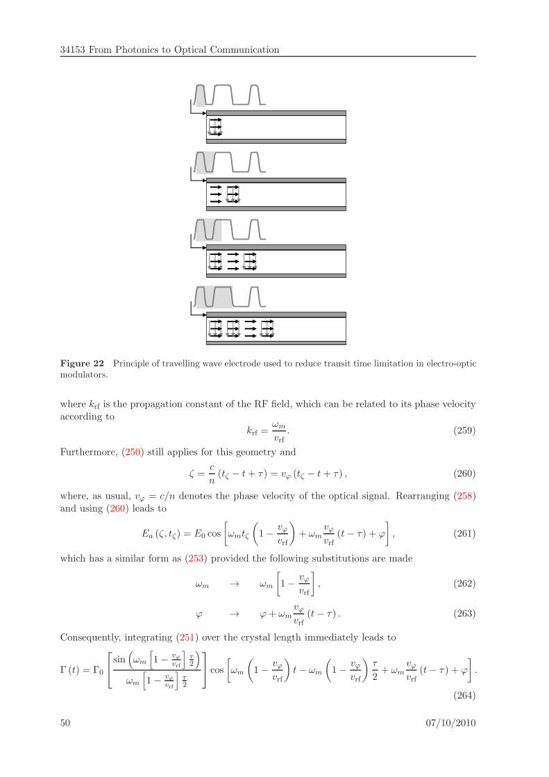
34153 From Photonics to Optical Communication
Figure 22 Principle of travelling wave electrode used to reduce transit time limitation in electro-opticmodulators.
where krf is the propagation constant of the RF field, which can be related to its phase velocityaccording to
krf =ωm
vrf. (259)
Furthermore, (250) still applies for this geometry and
ζ =c
n(tζ − t+ τ) = vϕ (tζ − t+ τ) , (260)
where, as usual, vϕ = c/n denotes the phase velocity of the optical signal. Rearranging (258)and using (260) leads to
Ea (ζ, tζ) = E0 cos
[ωmtζ
(1− vϕ
vrf
)+ ωm
vϕvrf
(t− τ) + ϕ
], (261)
which has a similar form as (253) provided the following substitutions are made
ωm → ωm
[1− vϕ
vrf
], (262)
ϕ → ϕ+ ωmvϕvrf
(t− τ) . (263)
Consequently, integrating (251) over the crystal length immediately leads to
Γ (t) = Γ0
sin(ωm
[1− vϕ
vrf
]τ2
)
ωm
[1− vϕ
vrf
]τ2
cos
[ωm
(1− vϕ
vrf
)t− ωm
(1− vϕ
vrf
)τ
2+ ωm
vϕvrf
(t− τ) + ϕ
].
(264)
50 07/10/2010
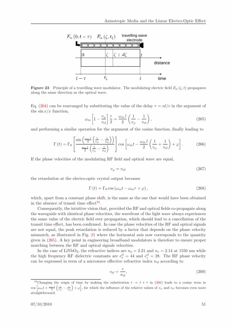
Anisotropic Media and the Linear Electro-Optic Effect
time
distance
travelling wave electrode
Figure 23 Principle of a travelling wave modulator. The modulating electric field Ea (ζ, t) propagatesalong the same direction as the optical wave.
Eq. (264) can be rearranged by substituting the value of the delay τ = nl/c in the argument ofthe sinx/x function,
ωm
[1− vϕ
vrf
]τ
2=
ωm l
2
(1
vϕ− 1
vrf
), (265)
and performing a similar operation for the argument of the cosine function, finally leading to
Γ (t) = Γ0
sin(ωm l2
(1vϕ
− 1vrf
))
ωm l2
(1vϕ
− 1vrf
)
cos
[ωmt− ωm l
2
(1
vϕ+
1
vrf
)+ ϕ
]. (266)
If the phase velocities of the modulating RF field and optical wave are equal,
vϕ = vrf, (267)
the retardation at the electro-optic crystal output becomes
Γ (t) = Γ0 cos (ωmt− ωmτ + ϕ) , (268)
which, apart from a constant phase shift, is the same as the one that would have been obtainedin the absence of transit time effect34.
Consequently, the intuitive vision that, provided the RF and optical fields co-propagate alongthe waveguide with identical phase velocities, the wavefront of the light wave always experiencesthe same value of the electric field over propagation, which should lead to a cancellation of thetransit time effect, has been confirmed. In case the phase velocities of the RF and optical signalsare not equal, the peak retardation is reduced by a factor that depends on the phase velocitymismatch, as illustrated in Fig. 21 where the horizontal axis now corresponds to the quantitygiven in (265). A key point in engineering broadband modulators is therefore to ensure propermatching between the RF and optical signals velocities.
In the case of LiNbO3, the refractive indices are no = 2.21 and ne = 2.14 at 1550 nm whilethe high frequency RF dielectric constants are ǫrfx = 44 and ǫrfz = 28. The RF phase velocitycan be expressed in term of a microwave effective refractive index nrf according to
vrf =c
nrf, (269)
34Changing the origin of time by making the substitution t → t + τ in (266) leads to a cosine term in
cos[
ωmt+ ωm l2
(
1vϕ
− 1vrf
)
+ ϕ]
, for which the influence of the relative values of vϕ and vrf becomes even more
straightforward.
07/10/2010 51

34153 From Photonics to Optical Communication
and it can be shown that
nrf =
√ǫrfr + 1
2, (270)
where ǫrf =√
ǫrfx ǫrfz is the relative dielectric constant of the material. In (270), the effective
relative permittivity ǫrfeff = n2rf can be seen as an average of the relative permittivity of the
medium and air, where the RF field propagates. In case the coplanar electrode is depositeddirectly on top of the LiNbO3 substrate, the value of the microwave effective index is thenequal to 4.25. Therefore the RF modulating field is slower than the optical field by a factor 2.Consequently, even when a travelling wave electrode configuration is used, the phase velocitymismatch between the RF field and the light wave will severely limit the bandwidth of electro-optic modulators based on LiNbO3. Hopefully some techniques have been devised to overcomethis inherent limitation. As already discussed in Sec. 4.1, using a silica buffer layer, whosedielectric constant is of the order of ǫ = 3.8, enables to reduce the velocity mismatch betweenthe RF and optical fields.
An imperfect match of the optical and RF phase velocities, vϕ 6= vrf, will result in walk-offbetween the phase fronts of the electrical and optical waves. This means that those two waveswill oscillate from in-phase to out-of-phase conditions, depending on the distance in the crystal,causing a reduction of the peak retardation. One way to overcome this limitation, at least atsome discrete design frequencies, is to engineer the interaction between the optical and RF wavesso that they never become out of phase [16]. This can be achieved by a proper configurationof the electrodes so that the direction of Ea in the waveguide is periodically reversed, or byensuring interaction between the optical and electrical fields only occurs close to the in-phasepositions. However, such designs are inherently bandpass, since the walk-off relation betweenelectrical and optical fields depends on the frequency of the modulating signal.
As discussed above, true velocity matching can be obtained provided the phase velocity ofthe RF wave can be increased by using a suitable buffer layer and electrode structure. Thekey to broadband operation for electro-optic modulators based on materials such as LiNbO3 istherefore the design of suitable structures that will furthermore present low microwave loss andimpedance matching. From a practical point of view, it is also desirable to achieve low voltageoperation, since it may be technically challenging, hence expensive, to design broadband highoutput voltage electrical amplifiers [17]. Low voltage operation can be achieved in principle byincreasing the electrode length. There is however a trade off between high bandwidth and lowvoltage operation since long electrodes will result in high microwave loss. A good review ofthe issues and challenges associated with the design of broadband electro-optic modulators inLiNbO3 can be found in [18]. So far, record bandwidths above 100 GHz have been reported forcarefully designed LiNbO3 modulators. For telecommunication applications, this is far beyondthe current requirement of about 30 GHz for the next generation systems that will operateat 40 Gbit/s. The use of other material systems, such as polymers, which have the benefitof simultaneously presenting a relatively high electro-optic coefficient and a small microwavedielectric constant that eases velocity matching, is also considered a promising and cost effectiveway to overcome bandwidth limitations.
So far, bandwidth limitations have been discussed assuming the modulating signal is a singlefrequency RF field. This has lead to the conclusion that, in order to overcome transit timelimitations, the phase velocities of the optical and RF fields should be matched. However, it isclear that once the modulation process has been initiated in the electro-optic crystal, the opticalwave is no longer strictly harmonic since it has become phase modulated. Furthermore, formost applications such as digital transmission, the modulating signal is no longer an harmonicfield, but a waveform where the information to be transmitted has been encoded under digitalor analogue form. For such non-harmonic signals, the velocity matching condition should be
52 07/10/2010

Anisotropic Media and the Linear Electro-Optic Effect
based on the group velocity instead of the phase velocity, as discussed for instance in [19, 20].
Appendices
A Light intensity
In this section, the concept of light intensity is clarified starting from the the energy consider-ations already discussed following the introduction of the Poynting vector in Sec. 1.4. Further-more, a relation is established between the electromagnetic formalism and standard expressionsemployed for the electric field in the context of optical modulation and the study of opticalcommunication systems in general.
A.1 Optical intensity
Starting from the the expression of the time average of the Poynting vector derived in (62),
〈S〉 = 1
2ωµ|E0|2 k, (271)
it is straightforward to derive and alternate expression
〈S〉 = 1
2η|E0|2 u, (272)
where η is the impedance of the medium (48). The optical intensity is defined as the magnitudeof the time averaged Poynting vector
I =1
2η|E0|2 , (273)
where the time averaging 〈〉 is performed over a duration that is long compared to an opticalcycle, but short compared to the variations of other physical quantities of interest.
In the context of the modulation of a light wave for optical communication systems applica-tions, wavelengths around 1550 nm are typically used, corresponding to frequencies of the orderof 193 THz, hence to a period of the optical carrier frequency equal to about 5.2 as. This valuehas to be compared to the characteristic duration of the quantity being modulated, which corre-sponds to either the inverse of the symbol rate for non return-to-zero (NRZ) modulation, or tothe pulse duration in case return-to-zero (RZ) modulation is used. For instance, in a standard40 Gbit/s NRZ system, the symbol duration is 25 ps, meaning that as many as 4825 opticalcycles are present in each symbol. The time averaging performed in order to define the intensityenables to follow the variations of the power envelope of the electric field, corresponding to theintensity modulation, but not those of the optical carrier.
Alternate expressions can be easily derived for the optical intensity. For instance, reporting(57) into (64) leads to
I =1
2ǫ vϕ |E0|2 , (274)
from which it is straightforward to derive another frequently used alternate form
I =1
2ǫ0 c n |E0|2 . (275)
07/10/2010 53

34153 From Photonics to Optical Communication
A.2 From the electromagnetism to the communications formalisms
In this section, a plane wave of the type
E (r, t) = ReE0 (r, t) ej(ωt−k·r)
, (276)
where E0 is a complex vector, is assumed to propagate in an isotropic medium. Defining anorthonormal basis (x,y, z), where z is the direction of propagation, E0 is in the plane orthogonalto z due to the transverse nature of the wave, and (276) can be expressed as
E (z, t) = ReE0 (z, t) ej(ωt−kz)
. (277)
The transverse vector E0 can be decomposed on (x,y) according to
E0 (z, t) = κ [ux (z, t)x+ uy (z, t)y] , (278)
where ux (z, t) and uy (z, t) are complex functions and κ is a normalisation constant. It is clearthat such an expression allows for the intensity, phase and polarisation of the light wave to betime dependent. The magnitude of E0 can be easily calculated
|E0|2 = E0 · E∗0 = κ2
[|ux (z, t)|2 + |uy (z, t)|2
], (279)
hence the light intensity
I (z, t) =1
2ǫ0 c nκ
2[|ux (z, t)|2 + |uy (z, t)|2
], (280)
and the optical power
P (z, t) =1
2ǫ0 c nκ
2A[|ux (z, t)|2 + |uy (z, t)|2
], (281)
where A corresponds to the area over which the intensity is integrated. The arbitrary normali-sation parameter κ can now be chosen so that the optical power is simply expressed as
P (z, t) = |ux (z, t)|2 + |uy (z, t)|2 . (282)
Consequently,
κ =
(2
ǫ0cnA
)1/2
, (283)
whose dimension is in√
Ω/m2.The coordinates of E0 along x and y in (278) can be further expressed in terms of their
magnitudes and phases, so that
E0 (z, t) = κ[Ax (z, t) e−jφx(z,t)x+Ay (z, t) e−jφy(z,t)y
], (284)
which immediately leads to
E0 (z, t) = κ e−jφ(z,t)[Ax (z, t) e−j
δ(z,t)2 x+Ay (z, t) ej
δ(z,t)2 y
], (285)
where
φ (z, t) =φx (z, t) + φy (z, t)
2(286)
54 07/10/2010

Anisotropic Media and the Linear Electro-Optic Effect
is the common phase, andδ = φx (z, t)− φy (z, t) (287)
is the differential phase term, which determines the state of polarisation of the wave. Introducingthe normalised Jones vector,
e (z, t) =1√
A2x (z, t) +A2
y (z, t)
[Ax (z, t) e−j δ(z,t)
2 x+Ay (z, t) ejδ(z,t)
2 y], (288)
enables to express the transverse field E0 as
E0 (z, t) = κ e−jφ(z,t)√A2
x (z, t) +A2y (z, t) e (z, t) , (289)
and thereforeE0 (z, t) = κ
√P (z, t) e−jφ(z,t) e (z, t) . (290)
E0 (z, t) is therefore proportional to the complex envelope of the field, multiplied by a unitvector describing the state of polarisation. In the study of optical modulation formats, theexplicit spatial dependence of the field is not always necessary, hence the following simplifiednotations will be adopted
E (t) = Reκ√
P (t) e−jφ(t) ejωt e (t), (291)
from which the various quantities that can be modulated, namely the power P (t), the phaseφ (t), the frequency ω and the polarisation e (t), are clearly visible. In order to simplify thenotations, the proportionality constant κ is often neglected in the optical communication liter-ature. This is of little consequence in practice. However, taking κ into account is necessary inorder to ensure that E has actually the dimension of an electric field (V ·m−1) in equations ofthe type (291). It can also be remarked that in the derivation above, the light wave is assumedto be polarised at any time, i.e. its state of polarisation is e (t) at time t, even though it isnot single frequency due to the time varying term E0 (z, t) in (277), but has a narrow spectrumcentred around the carrier frequency ω.
B On the reduction of quadratic forms
We consider the second order surface (Σ) defined by the following equation in a Cartesiancoordinate system (O, e1, e2, e3), where e = (e1, e2, e3) is an orthonormal basis:
a11x2 + a22y
2 + a33z2 + 2a23yz + 2a13xz + 2a12xy + b1x+ b2y + b3z + c = 0. (292)
Such a surface is known as a quadratic surface or quadric. Depending on the values of thecoefficients, (292) can describe an ellipsoid, an hyperboloid of one or two sheets, an elliptic cone,an elliptic paraboloid, an hyperbolic paraboloid, an elliptic cylinder, an hyperbolic cylinder, aparabolic cylinder, one or two parallel planes, a line, a point, or the empty set. Quadrics canbe classified according to the properties of the eigenvalues of the associated quadratic form. Inour study of anisotropic media and the electro-optic effect, we will be primarily concerned withthe case of ellipsoids. Here we show how the general equation (292) can be reduced to a morefamiliar canonical expression.
The quadratic form associated to (Σ) is
q (x, y, z) = a11x2 + a22y
2 + a33z2 + 2a23yz + 2a13xz + 2a12xy, (293)
07/10/2010 55

34153 From Photonics to Optical Communication
whose matrix in the basis e is
Q =
a11 a12 a13a12 a22 a23a13 a23 a33
. (294)
We can therefore express the quadratic form q according to
q (x, y, z) = xTQ x, (295)
where x is the column vector x =(x y z
)Tand T denotes the transposition operation. To
simplify the notations, the equation of the surface (Σ) can be written in vectorial form
xTQ x+ bTx+ c = 0, (296)
where bT =(b1 b2 b3
).
Q is a symmetric matrix whose elements are real. Hence there exists an orthonormal basise = (e1, e2, e3) where the quadratic form q is represented by a diagonal matrix
Λ =
λ 0 00 µ 00 0 ν
, (297)
such that Λ = P TA P , where P is the transformation matrix from the basis e to the neworthonormal basis e, and λ, µ and ν are the eigenvalues of Q.
We can write the equation of (Σ) in the new basis by performing the transformation x = P x.We immediately obtain
xTΛ x+ bTP x+ c = 0. (298)
If we perform the extra transformation ¯x = x − a, which corresponds to a change of origin ofthe coordinate system (translation by a), the equation of (Σ) becomes
¯xTΛ ¯x+(2aTΛ+ bTP
)¯x+ aTΛ a+ bTP a+ c = 0. (299)
Provided none of the eigenvalues of Q is equal to 0, the linear terms of the equation can besuppressed by a careful choice of a so that 2aTΛ + bTP = 0T . In this case, it is immediatelyfound that (Σ) has an equation of the type
λ¯x2 + µ¯y2 + ν ¯z2 + γ = 0, (300)
where γ is a constant, in the new coordinate system. If the three eigenvalues λ, µ and ν havethe same sign, then (Σ) is either the empty set or an ellipsoid. In the later case, believed to beof significantly higher interest, the equation of the surface can be further reduced to the wellknown canonical form (
¯x
x0
)2
+
(¯y
y0
)2
+
(¯z
z0
)2
= 1. (301)
The following special cases may be further distinguished:
• If all three eigenvalues are equal, λ = µ = ν, then (Σ) is a sphere.
• If Q has only 2 distinct eigenvalues, e.g. λ = µ 6= ν, then (Σ) is an ellipsoid of revolution.
It can also easily be shown that the intersection of a quadric with a plane is a conic. In thecase of an ellipsoid, this intersection is an ellipse. This property has been exploited in Sec. 2.3for the geometrical determination of the normal modes of propagation from the index ellipsoid.
56 07/10/2010
Anisotropic Media and the Linear Electro-Optic Effect
References
[1] M. Born and E. Wolf, Principles of Optics, Pergamon Press, Oxford, sixth edition, 1993.
[2] P. N. Butcher and D. Cotter, The Elements of Nonlinear Optics, chapter 2, pp. 12–36,Cambridge Studies in Modern Optics. Cambridge University Press, Cambridge, 1990.
[3] L. D. Landau, E. M. Lifshitz, and L. P. Pitaevskii, Electrodynamics of Continuous Media,chapter 9, pp. 257–289, Butterworth-Heinemann, Oxford, second edition, 1984.
[4] P.-H. Tsao, “Derivation and implications of the symmetry property of the permittivitytensor”, American Journal of Physics, vol. 61, no. 9, pp. 823–825, 1993.
[5] I. P. Kaminow, An Introduction to Electrooptic Devices, Academic Press, New York, 1974.
[6] E. Hartmann, “An introduction to crystal physics.” International Union of Crystallography,University College Cardiff Press, Cardiff, Wales, U.K., 1984.
[7] E. H. Turner, “High-frequency electro-optic coefficients of lithium niobate”, Applied Physics
Letters, vol. 8, no. 11, pp. 303–304, 1966.
[8] R. S. Weis and T. K. Gaylord, “Lithium niobate: summary of physical properties andcrystal structure”, Applied Physics A, vol. 37, no. 4, pp. 191–203, 1985.
[9] A. Donaldson, “Candidate materials and technologies for integrated optics: fast and ef-ficient electro-optic modulation”, Journal of Physics D: Applied Physics, vol. 24, no. 6,pp. 785–802, 1991.
[10] M. Lawrence, “Lithium niobate integrated optics”, Reports on Progress in Physics, vol. 56,no. 3, pp. 363–429, 1993.
[11] E. L. Wooten, K. M. Kissa, A. Yi-Yan, E. J. Murphy, D. A. Lafaw, P. F. Hallemeier,D. Maack, D. V. Attanasio, D. J. Fritz, G. J. McBrien, and D. E. Bossi, “A review oflithium niobate modulators for fiber-optic communication systems”, IEEE Journal of Se-
lected Topics in Quantum Electronics, vol. 6, no. 1, pp. 69–82, 2000.
[12] C. M. Kim and R. V. Ramaswamy, “Overlap integral factors in integrated optic modulatorsand switches”, Journal of Lightwave Technology, vol. 7, no. 7, pp. 1063–1070, 1989.
[13] R. C. Alferness, “Waveguide electrooptic modulators”, IEEE Transactions on Microwave
Theory and Techniques, vol. MTT-30, no. 8, pp. 1121–1137, 1982.
[14] W. W. Rigrod and I. P. Kaminow, “Wide-band microwave light modulation”, Proceedingsof the IEEE, vol. 51, no. 1, pp. 137–140, 1963.
[15] C. J. Peters, “Gigacycle bandwidth coherent light traveling-wave phase modulator”, Pro-ceedings of the IEEE, vol. 51, no. 1, pp. 147–153, 1963.
[16] R. C. Alferness, S. K. Korotky, and E. A. Marcatili, “Velocity-matching techniques for in-tegrated optic traveling wave switch/modulators”, IEEE Journal of Quantum Electronics,vol. QE-20, no. 3, pp. 301–309, 1984.
[17] M. Doi, M. Sugiyama, K. Tanaka, and M. Kawai, “Advanced LiNbO3 optical modulatorsfor broadband optical communications”, IEEE Journal of Selected Topics in Quantum
Electronics, vol. 12, no. 4, pp. 745–750, 2006.
07/10/2010 57

34153 From Photonics to Optical Communication
[18] M. M. Howerton and W. K. Burns, RF photonics technology in optical fiber links, chapter 5:“Broadband traveling wave modulators in LiNbO3”, pp. 133–164, Cambridge UniversityPress, Cambridge, 2002.
[19] I. P. Kaminow and J. Liu, “Propagation characteristics of partially loaded two-conductortransmission line for broadband light modulators”, Proceedings of the IEEE, vol. 51, no. 1,pp. 132–136, 1963.
[20] R. Spickermann, S. R. Sakamoto, and N. Dagli, “In traveling wave modulators whichvelocity to match?”, in IEEE Lasers and Electro-Optics Society Annual Meeting, LEOS’96,paper WM3, vol. 2, pp. 97–98, 1996.
Problems
Problem 1
Derive the Helmholtz equation (41) for the electric field.
Problem 2
Derive the expression of the time averaged electric energy density (81) in the case of ananisotropic and non dispersive medium.
Problem 3
Bi12SiO20, also known as BSO, is an example of crystals that are naturally isotropic but thatbecome anisotropic under the influence of an external applied electric field. Its electro-optictensor is
r23 =
0 0 00 0 00 0 0r41 0 00 r41 00 0 r41
(302)
1. Write an expression for the index ellipsoid of BSO in an orthonormal basis (x,y, z) in theabsence of any external field.
2. An external electric field Ea is now applied to the crystal. Write how this field modifiesthe index ellipsoid of BSO.
3. It is assumed in particular that the applied electric field is parallel to x. Find the directionsof the new eigenmodes of propagation and associated refractive indices.
4. Assuming the crystal is used in the longitudinal configuration, find an expression for thehalf-wave voltage. Calculate the value of this voltage at 633 nm assuming n0 = 2.53 andr41 = 3.6× 10⁻¹² m/V.
58 07/10/2010
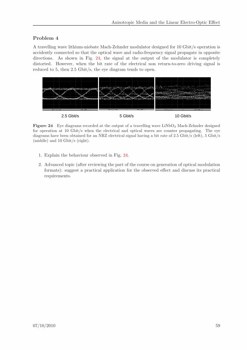
Anisotropic Media and the Linear Electro-Optic Effect
Problem 4
A travelling wave lithium-niobate Mach-Zehnder modulator designed for 10 Gbit/s operation isaccidently connected so that the optical wave and radio-frequency signal propagate in oppositedirections. As shown in Fig. 24, the signal at the output of the modulator is completelydistorted. However, when the bit rate of the electrical non return-to-zero driving signal isreduced to 5, then 2.5 Gbit/s, the eye diagram tends to open.
2.5 Gbit/s 10 Gbit/s5 Gbit/s
Figure 24 Eye diagrams recorded at the output of a travelling wave LiNbO3 Mach-Zehnder designedfor operation at 10 Gbit/s when the electrical and optical waves are counter propagating. The eyediagrams have been obtained for an NRZ electrical signal having a bit rate of 2.5 Gbit/s (left), 5 Gbit/s(middle) and 10 Gbit/s (right).
1. Explain the behaviour observed in Fig. 24.
2. Advanced topic (after reviewing the part of the course on generation of optical modulationformats): suggest a practical application for the observed effect and discuss its practicalrequirements.
07/10/2010 59