Physics 182

Electrostatics I

Fields.

Electrodynamics is a field theory. What does that mean?

The idea of a physical field developed slowly in the first half of the 19th century, as phenomena apparently acting “at a distance” were subjected to close study. Those phenomena included gravity, electricity and magnetism, through which objects interacted with each other with no apparent contact between them.

The idea of a field started with the belief that there must be something going on in the space between the interacting objects, something that transmits the observed effects. In a search for a pictorial conception, a mysterious “medium” was invented to “transport” the effect from the “source” to the “object” of the force. This medium was, of course, invisible. One could also walk through it without sensing its presence. Nevertheless, it could transmit (very quickly) information about the status of the source to the object, even if the latter was a large distance away.

When it became clear about 1820 that light is a wave phenomenon, it was natural to assume that the same mysterious medium that carries light waves is the one that transmits electric, magnetic, and perhaps gravitational forces. But there was a problem. The speed of waves in a medium increases with the “stiffness” of the medium; the speed of sound is much larger in a steel rod than in air. But the speed of light is extremely large, so the presumed medium must be extremely stiff. How then can one walk through it and not know it is there? Nevertheless, lacking a better explanation, the existence of this medium (called the luminiferous æther) was a common assumption in 19th century physics.

The æther could undergo stresses, strains and vortex motions, resulting in the propagation of waves and the transmission of forces. To study the state of the material (whatever it might be) in the æther was of obvious importance. That state involved physical properties, and the idea that physical properties could be attributed to points in apparently empty space was a crucial first step toward the idea of fields.

In fact, what we now call a field is just an entity in which some kind of physical property is distributed in space, having a value at each point. But we no longer try to associate that physical property with a substance filling the space. We reduced the theory of the æther to the status of historical myth, but we kept the idea of a field.

1

To define a field, we simply give some plausible way to measure its value at each point. The field of temperatures at various locations on the earth’s surface is defined by the method of measuring the value of the temperature at a location. This is an example of a scalar field, because temperature is a scalar quantity.

The main fields we will deal with in this course are those associated with electric and magnetic forces; since force is a vector, these are vector fields. We will also introduce some auxiliary fields called potentials; one is a scalar, the other a vector.

The electric field.

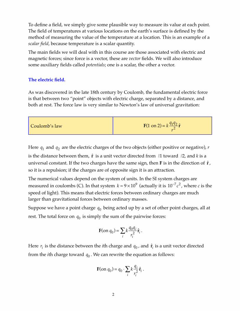
As was discovered in the late 18th century by Coulomb, the fundamental electric force is that between two “point” objects with electric charge, separated by a distance, and both at rest. The force law is very similar to Newton’s law of universal gravitation:

Coulomb’s law F(1 on 2) = k q1q2

r2 r̂

Here q1 and q2 are the electric charges of the two objects (either positive or negative), r

is the distance between them, ̂r is a unit vector directed from #1 toward #2, and k is a universal constant. If the two charges have the same sign, then F is in the direction of ̂r , so it is a repulsion; if the charges are of opposite sign it is an attraction.

The numerical values depend on the system of units. In the SI system charges are measured in coulombs (C). In that system k ≈ 9 × 109 (actually it is 10−7c2 , where c is the speed of light). This means that electric forces between ordinary charges are much larger than gravitational forces between ordinary masses.

Suppose we have a point charge q0 being acted up by a set of other point charges, all at

rest. The total force on q0 is simply the sum of the pairwise forces:

F(on q0 ) = k q0qi

ri2 r̂i

i∑ .

Here ri is the distance between the ith charge and q0 , and ̂ri is a unit vector directed

from the ith charge toward q0 . We can rewrite the equation as follows:

F(on q0 ) = q0 ⋅ k qi

ri2 r̂i

i∑ .

2

If q0 is moved to a different point in space the quantity represented by the sum will be

different, because the r’s will be different. So the equation can also be written as

F(on q0 at P) = q0 ⋅E(P) .

Here P stands for a point in space where q0 is located. The vector E(P) depends on the

other charges, where they are, and the point P, but not on the value of q0 . This quantity

is called the electric field at point P. The qi are called the source charges, and their

locations are the source points.

The proper definition of the field, which stresses how it is measured, is this:

Electric field definition

1. Place q0 at P, at rest.

2. Measure F(on q0 at P) .

3. Then E(P) = F(on q0 at P)

q0

If the sources of this field are charges at rest, then it is an electrostatic field. But, as we will see later, there are electric fields satisfying the above definition that do not arise from charges at rest. For now we treat only the electrostatic field.

Is it necessary to introduce this field? Not if all we ever do is treat charges at rest. But later we will see that the field has an independent existence, possessing energy and momentum. And even in the treatment of charges at rest it is a great convenience to divide the interaction of a given charge with other charges in two steps: (1) the other charges set up the field; (2) the given charge experiences their effect through the field.

Finding the field by superposition.

The electric field (which we will call the E-field) obeys a principle of superposition, which means that if there are multiple sources the total field is the (vector) sum of the fields of the separate sources. The sum used above is an example.

Let us clarify the notation for such sums. We will use the symbol r to represent the field point, the point in space where we are evaluating the field. We will use r’ to represent a source point, the location of a source charge. We will denote the displacement of the field point from the source point by R = r − ′r .The text by Griffiths (G) uses a script “r” for this displacement.

3

In this notation, the contribution of a source charge qi located at source point ′ri to the

E-field at field point r is:

Ei(r) = kqi

R iRi

3 .

Here we have used the fact that a unit vector in the direction of R i can be written out as

R i /Ri . The total field at r due to a set of sources is

E(r) = k qi

R iRi

3i∑ . (1)

This is all for point charge sources. Often we will treat the sources as a continuous distribution of charge, with charge per unit volume ρ( ′r ) . The total field is then given by an integral over the region of space containing the sources:

E(r) = k ρ( ′r ) R

R3 d3 ′r∫ (2)

where R = r − ′r , and the integration is over the volume containing all points where ρ

is not zero. (We use d3r to denote an element of volume. G uses dτ for this.)

Eqs (1) and (2) provide one method for calculating E. It must be remembered that the sum or integral is adding up vectors.

General properties of the electrostatic field: the divergence.

A vector field is specified uniquely by the values of its divergence and curl, except for a possible additive uniform field (one that is the same everywhere). So we will examine those two quantities.

First the divergence. One must be careful because simply calculating ∇ ⋅E(r) = ∂iEi(r)

seems to give the result zero.Actually it is indeterminate at the location of the source charges.

Instead we will use the divergence theorem:

∇ ⋅Ed3r∫ = E ⋅dA∫ .

Here the volume integral covers a region of space bounded by the surface in the area integral, and dA is an element of that area, directed outward from the enclosed volume.

4

The area integral (the total flux of the field through the surface of the region) gives a simple result if the source is a single (positive) point charge q at the origin. First, we note that the direction of E is radially outward. The infinitesimal contribution to the flux by the surface element dA can be written as E(r) ⋅dA = Ecosα ⋅dA , where α is the angle between the outward normal to the surface element and the direction of E (which in this case is the same as the direction of r).

The geometry is shown. The element of surface area perpendicular to r is

dA⊥ = r2 ⋅dΩ , where dΩ is the element of solid angle subtended at the

origin by dA⊥ ; this is the set of angular displacements indicated by the

dotted lines in the drawing. In spherical coordinates the solid angle element takes the form dΩ = sinθ dθ dφ . See the

section on curvilinear coordinates in Chap. 1 of G.

But since dA⊥ = dA ⋅cosα , we find

E ⋅dA = E ⋅dA⊥ =

kqr2 ⋅ r2dΩ = kq ⋅dΩ .

The total flux through a closed surface surrounding the charge is

E ⋅dA∫ = kq dΩ∫ = 4πkq .

We have used the fact that the integral of dΩ over all directions is 4π .

To prove this, use the formula above in spherical coordinates, and note that all directions are covered by the ranges 0 ≤ θ ≤ π and 0 ≤ φ ≤ 2π .

So a single point charge q within the volume bounded by the closed surface gives a contribution 4πkq to the flux outward. By superposition, if we have a number of

charges within that volume, the total flux is 4πk qi

i∑ = 4πk ⋅Qtot . The net flux from

charges not enclosed in the volume is zero, because cosα is negative as much as positive. The final result is called Gauss’s law:

Gauss’s law (integral form) E ⋅dA∫ = 4πk ⋅Qtot

Here Qtot is the total charge in the volume enclosed by the surface.

Notation: it is common to write the universal constant k as 1/ 4πε0 , in which case 4πk = 1/ε0 . This is the

notation used in G.

r dA

α

5

Now we return to the question of ∇ ⋅E . We write the total charge in the volume as

Qtot = ρd3r∫ , where the integral covers the volume bounded by the surface. On the

other hand, the divergence theorem says E ⋅dA∫ = ∇ ⋅Ed3r∫ . So Gauss’s law tells us

that ∇ ⋅Ed3r∫ = 4πk ρd3r∫ , where the integrals on the two sides cover the same volume.

This implies

Gauss’s law (differential form) ∇ ⋅E = 4πkρ

The integral form makes it easier to include both point charges and continuous distributions in the law. For a true point charge, ρ is zero except at the location of the charge, where it is infinite. This makes the

differential form of the law a bit awkward to use directly. One handles this difficulty by use of the Dirac delta function, discussed in Chap. 1 of G.

General properties of the electrostatic field: the curl.

It is easier to calculate the ∇ × E for the electrostatic field. Consider the field of a point charge at the origin: E(r) = kq ⋅ r /r3 . This has the form f (r) ⋅ r , and the curl of any such

function is zero.

Proof: Write the curl as ε ijkl∂ j[ f (r) ⋅ rk] . Do the derivative:

∂ j f (r) ⋅ rk = ′f (r) ⋅ (∂ jr) ⋅ rk + f (r) ⋅ ∂ jrk = ′f (r) ⋅ (rj /r) ⋅ rk + f (r) ⋅δ jk . This object is

unchanged when the indices j and k are interchanged. But ε ijk changes sign under that

interchange of indices, so the curl is equal to minus itself, therefore zero.

The conclusion is a fundamental property:

Curl of the electrostatic field ∇ × E = 0

We can convert this into integral form by using Stokes’s theorem:

E ⋅dr∫ = (∇ × E) ⋅dA∫ .

Here the line integral is called the circulation. The curve integrated over is the boundary of the surface integrated over on the right side. Applying this we have

6

Circulation of the electrostatic field E ⋅dr∫ = 0

These two properties, expressed here in both integral and differential form, are fundamental aspects of the electrostatic field.

Electric potential.

Since the curl of any function that is the gradient of a scalar function is automatically zero, we can write the electrostatic field as such a gradient. We define:

Electric potential (differential form) E = −∇V

The negative sign is for convenience later. The integral form of this is:

Electric potential (integral form) V(r2 ) −V(r1) = − E ⋅dr

r1

r2∫

If one can calculate V, then the first form of the definition can be used to find E. If one can calculate E, then the second form can be used to find V.

Because adding a constant to V everywhere does not alter the fact that it satisfies the definitions, specifying V completely requires making a choice as to its value at a particular point. There are conventional choices, however. For example, if all the source charges for the fields are confined to a finite region of space, then V is usually taken to be zero at infinite distance from that region. Or perhaps it will be set to zero on some conductor in the situation.

The potential is a scalar field. As a result it is often easier to calculate for given source charges than E. The direct method is like the one used for E: find the formula for the field of a point source, then use superposition.

Let the source be a point charge at the origin. Then we know E:

E(r) = kq r

r3 .

The integral form above then gives

7

V(r) −V(r0 ) = − kq ′r

′r 3 ⋅d ′rr0

r∫ ,

where r0 is a reference point at which we will assign a particular value to V. The line

integral follows some path from r0 to r, but any path will give the same answer as any

other, so we can choose the simplest. We choose r0 to be infinitely far away, set V = 0 at

that distance, and choose a path along a line straight toward the origin. Then in the integrand ′r and d ′r will both be along that line, so ′r ⋅d ′r = ′r d ′r . This gives

V(r) = − kq d ′r

′r 2∞

r∫ =

kqr

.

That this result depends only on the distance from the source charge and not on the direction is a consequence of the symmetry. We have found our answer:

Potential of point charge V(r) = kq

r

If there are several point charges we note that the contribution of one of them to the potential at a particular field point depends only on the charge and its distance from that point. Using superposition we find:

V(r) = kqi

r − rii∑ . (3)

If the source charges are continuously distributed, this becomes an integral:

V(r) = k ρ( ′r )

r − ′rd3 ′r∫ . (4)

It should be remembered that in all these formulas we have chosen V(∞) = 0 . Other choices would result in adding a constant to V.

Because potential involves an arbitrary choice of its value at some point, it is not directly measurable. Only differences in potential between different points are measurable. The E-field, on the other hand, is directly measurable.

Energy in electrostatics.

The Coulomb force is a central force, therefore conservative. So there is potential energy associated with it. As usual, one can find the potential energy difference between two

8

states in two equivalent ways: (1) Calculate the work done by the force itself in moving the system from rest in the initial state to rest in the final state; the potential energy change is the negative of this work. (2) Calculate the work done by an external agent in make the same change of the state of the system; the potential energy change is this work. Both ways of finding the change are useful.

Taking the first point of view, assume the E-field is known. Now take a “test” charge q0

at point A (at rest) and let the force F = q0E move it to point B (also at rest). The work

done is W(A → B) = q0E(r) ⋅dr

A

B∫ . This is minus the change in potential energy, so

U(B) −U(A) = − q0E(r) ⋅dr

A

B∫

But the right side is just q0[V(B) −V(A)] , so we have

Relation of U to V ΔU = q0ΔV

We must interpret this simple equation carefully. It says that if a charge q0 is moved

through a potential difference ΔV in a field due to other charges, then the potential energy of the whole system (sources of the field and q0 ) changes by the amount q0ΔV . As q0

moves the other charges must remain fixed so that their field does not change.

Now we look at the energy “stored” in a system of charges due to the electrostatic interaction. For this purpose it helps to take the other point of view about potential energy, that is is the work done by an external agent to put the charges in their places.

Consider first a pair of point charges, q1 and q2 . Initially let them be infinitely far away

and from each other, and define this state to have potential energy zero. We ask for the potential energy when q1 is at location r1 and q2 is at r2 . First we move q1 to its final

location r1 ; since there is no interaction with the other charge, it requires no work to do

this, but now there is a potential kq1 /r at every point at distance r from this charge.

Then we move q2 to r2 ; the work done is the change in potential energy of the system,

which by the above formula is

U = q2ΔV = q2V1(r21) = k q2q1

r21.

9

Here r21 = r2 − r1 is the distance from q1 to q2 , and V1(r21) is the potential of q1 at

distance r21 from it. What we have calculated is the potential energy change while q2 is

moved from infinity to a point at distance r21 away from q1 , which was held fixed.

If we had brought in q2 first, then held it fixed while we brought in q1 , the result would

have been

U = q1V2(r12 ) = k q1q2

r12.

But r12 = r21 , so the potential energy change would have been the same. The total

potential energy depends only on the final configuration of the charges, not on the order in which they were put in place.

We emphasize this symmetry by writing the answer as

U = 12 [q1V2(r12 ) + q2V1(r21)] .

This shows how to generalize to more charges:

Potential energy of point charges U = 1

2 qiV(at qi )i∑

Here V(at qi ) is the potential at the location of qi due to all the other charges.

If the charge is a continuous distribution this becomes an integral:

Potential energy for a continuous distribution of charge U = 1

2 ρ(r∫ )V(r)d3r

The potential energy here is that of static charges, held in place somehow. If the charges are set free, they will move. If the total potential energy is positive, they will move away from each other; if the potential energy is negative they will move toward each other. If the system is one of point charges interacting only by the Coulomb forces, one can show (Earnshaw’s theorem) that no configuration of stable equilibrium exists.

We can recast the formula for total potential energy of a system of charges entirely in terms of the E-field. We start from the expression immediately above. Putting E = −∇V into Gauss’s law we find Poisson’s equation for V:

10

Poisson’s equation ∇2V = −4πkρ

Here ∇2V = ∇ ⋅∇V , or ∇2V = ∂i∂iV . We use this to solve for ρ and substitute into the

formula for potential energy of a continuous distribution (above), obtaining

U = −

18πk

V ⋅∇2V d3r∫ .

Now we note that ∇ ⋅ (V∇V ) = ∂i(V∂iV ) = (∂iV )(∂iV ) +V(∂i∂iV ) = E2 +V ⋅∇2V , so

V ⋅∇2V = ∇ ⋅ (V∇V ) − E2 . Then we have

U =

18πk

[E2 − ∇ ⋅ (V∇V )]d3r∫ .

Let us examine the 2nd term in the integral. By the divergence theorem it is proportional to

(V∇V ) ⋅dA∫ . This is the flux of the quantity V∇V through a surface

surrounding all space, i.e., at infinite distance. Think of it as a sphere of radius R as R →∞ . The surface area is proportional to R2 . But the potential of any charge distribution confined to a finite region of space will decrease with distance at least as fast as R−1 , and ∇V will decrease at least as fast as R−2 . So V∇V decreases with

distance at least as fast as R−3 . The integral must then be proportional to R−1 or smaller. As R →∞ it vanishes.

Our final result is:

Potential energy in E-field U =

18πk

E2 d3r∫

The integral covers all space. The quantity E2 /8πk give the energy per unit volume

associated with the electric field. This is called the energy density:

Energy density in E-field ηe =

18πk

E2 = 12 ε0E2

These formulas give a way of calculating the potential energy directly from the E-field. More importantly, they show that the field possesses energy, with density proportional to the square of the field strength.

11

Conductors in electrostatics.

It was found in the 18th century that metals and some other materials can convey charge from one place to another, and, if isolated from other bodies, can keep charge stored. These are conductors. We are not concerned here with the flow of charge by means of conductors, but rather with the situation when all charges are at rest, in what is called electrostatic equilibrium.

There are several ways to place charge on an isolated conductor:

• Bring into physical contact an already charged object. Some of its charge will flow onto the conductor, and remain there when the object is removed.

• Charge by induction, bringing, say, a positively charged object near the conductor. This will attract negative charge to the near side of the conductor, leaving the far side with net positive charge. Then bring a second conductor (such as a wire attached to the earth) into contact with the far side of the conductor. Positive charge will flow off. When the wire is removed the conductor will have net negative charge.

• Put another charged conductor nearby that creates an E-field so intense that the air molecules are ripped apart and the air itself becomes a conducting path to carry charge to the original conductor.

Suppose we have a charged conductor, and the charge has been distributed so that it has come to rest. What can we say about the E-field and the distribution of charge?

First, what makes a material a conductor? We consider only solids here. When atoms or molecules arrange themselves so tightly bound as to make a solid, the nature of the states of the least tightly bound electrons is altered. In some materials those electrons remain identified with individual atoms, but in some they become common property, able to move around in the material. In the former case it takes a very large external E-field to make any electrons break free from their atoms; these are non-conductors. In the latter case, a very small E-field can make some the electrons move (opposite to the direction of the field, because they have negative charge); these are conductors.There is not a complete dichotomy here, but a continuum. The ability of electrons to move varies and is measured by the conductivity of the material. For our purposes here we assume a conductor has a very high conductivity. There are in fact (at very low temperatures) superconductors with infinite conductivity.

So what distinguishes a conductor is the fact that any weak external E-field will make charges move within the material or along its surface. It follows that:

If all charges are at rest, there can be no E-field within the material or along its surface.

There can, however, be an E-field at the surface directed perpendicular to it, because the electrons are not free to leave the conductor. So:

If all charges are at rest, any E-field at the surface must be perpendicular to it.

12

Now we look at the distribution of charge. The tool to use is Gauss’s law in integral form:

E ⋅dA∫ = 4πk ⋅Qtot .

First, the charge within the conductor. Choose for the “Gaussian” surface to be used on the left side of Gauss’s law the dotted surface shown, below the surface of the conductor. Because it is entirely within the conductor, the E-field is zero everywhere on it, so the flux integral is zero. This means the total charge enclosed is zero. We could shrink this surface to surround any region within the conductor and the conclusion would be the same. Or we could expand it until it lies just beneath the actual surface of the conductor. So we conclude:

There is no net charge within a conductor , if all charges are at rest.

This means any charge there is must reside on the surface(s) of the conductor. How it is distributed is related to the E-field (if any) at the surface. We examine this connection.

Shown is part of the top surface of a conductor. We construct a “pillbox” Gaussian surface as shown: its is top above the conductor surface, its bottom is embedded in the conductor, and its sides are perpendicular to the conductor surface. Consider the flux through this pillbox. The flux through the bottom is zero, because the E-field is zero within the conductor. The flux through the sides it is zero because the field is either zero (within the conductor) or parallel to the sides, so that E ⋅dA = 0 ( dA is perpendicular to the surface). This leaves only the top. Call its area A. If the pillbox is very small the E-field is the same across the area of the top; because it is perpendicular to the conductor surface it is parallel to dA . So the flux through the top is E ⋅ A . The total charge enclosed in the pillbox is the charge on that part of the surface inside the pillbox. Call the charge per unit area σ . Then the enclosed charge is σ ⋅A . Putting these facts into Gauss’s law we find E ⋅ A = 4πk ⋅σ ⋅ A , or:

If all charges are at rest, the E-field at the surface of a conductor is related to the charge per unit area by E = 4πk ⋅σ = σ /ε0 .

Finally, we consider the potential at points on the conductor. We use the definition:

V(r2 ) −V(r1) = − E ⋅dr

r1

r2∫ . Let both points be on or in the conductor. We can take a path

between them that either goes within the conductor (where E = 0 ) or along the surface (where E ⊥ dr ). Either way, the line integral is zero, so the two points are at the same potential:

If all charges are at rest, all points on or in a conductor are at the same potential.

These are the five important properties of a conductor in electrostatics.

13