1

Electronic Supplementary Information for:

Pseudo-tetrahedral vs pseudo-octahedral ErIII single molecule magnets and the disruptive role of coordinated TEMPO radicals

Maria Brzozowska, Gabriela Handzlik, Katarzyna Kurpiewska, Mikołaj Zychowicz and Dawid Pinkowicz*Jagiellonian University, Faculty of Chemistry, Gronostajowa 2, 30-387 Kraków, Poland

Electronic Supplementary Material (ESI) for Inorganic Chemistry Frontiers.This journal is © the Partner Organisations 2021

2

Experimental sectionGeneral synthesis considerationsAll manipulations were performed under inert gas atmosphere inside an argon filled glovebox (Inert PureLab HE). All solvents used in this study (HPLC grade) were dried under argon using Inert PureSolv EN7 solvent purification system. Anhydrous ErCl3 (at least 99.9%) was purchased from Alfa Aesar and used as received. Li3(N3N) was prepared according to the previously published method.1 Sodium 2,4,6-tri-tert-butyl-phenolate (NaTTBPEt2O) and sodium 2,6-di-tert-butyl-4-methylphenolate (NaBHTEt2O) were prepared by slowly adding dry sodium hydride to the Et2O solution of the respective phenol (Sigma Aldrich, 98%) inside the glovebox. See below for a detailed procedure. NaTTBPEt2O obtained in this way is identical with that obtained using a slightly different method reported in the literature.2

Preparation of sodium 2,4,6-tri-tert-butyl-phenolate (NaTTBPEt2O)2,4,6-tri-tert-butyl-phenol (10.7 g, 40 mmol) was dissolved in 40 ml of dry Et2O (bright yellow solution) and heated to boiling. NaH (0.912 g, 38 mmol) was added in small portions while stirring. Each portion causes vigorous gas evolution. Stirring was continued for another 1.5 h after the last portion of NaH was added. The off-white crystalline precipitate was collected by filtration (the filtrate is yellow) and washed with three portions of Et2O. Yield 10.95 g (80 %). NaTTBPEt2O obtained in this way is identical with that obtained using a slightly different method reported in the literature.2

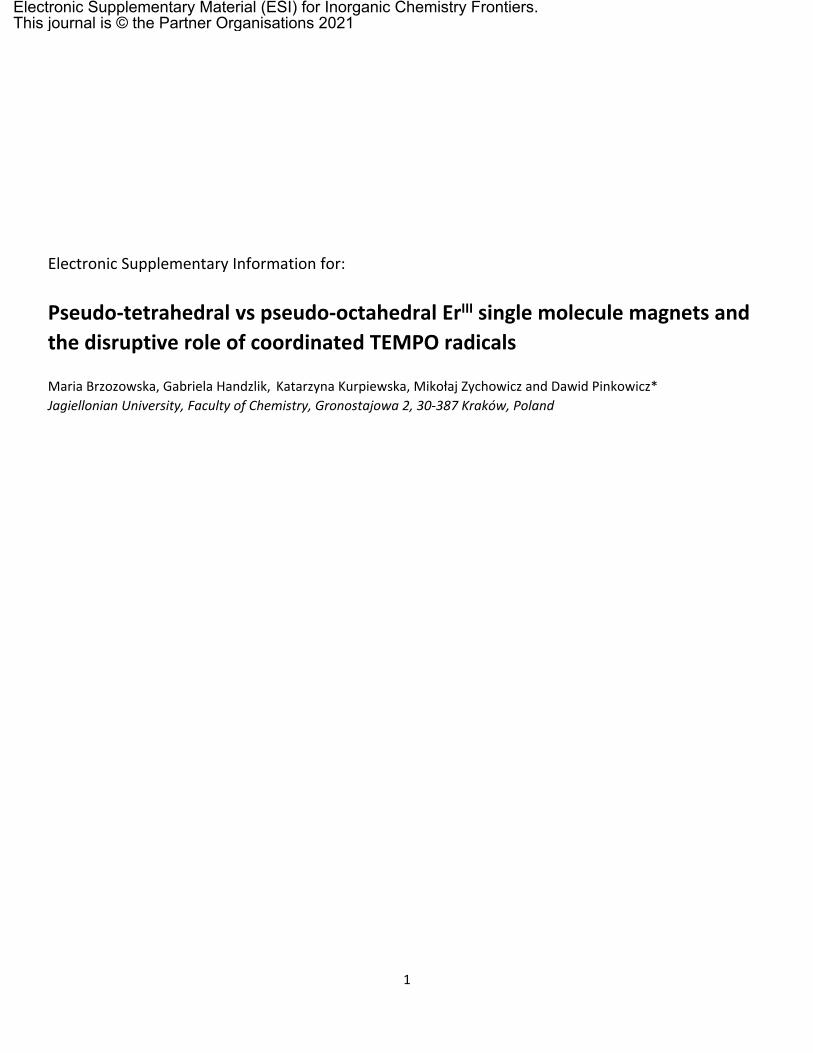
Preparation of [ErIII(TTBP)3(THF)] (1)NaTTBPEt2O (3.89 g, 10.9 mmol) and ErCl3 (1.03 g, 3.65 mmol) were suspended in 40 ml of THF. The pink reaction mixture was stirred for 3 days and then the solvent was removed in vacuo. The pink residue was suspended in 50 ml of pentane, stirred for 30 min and then left to settle. Then pink solution was decanted and filtered through a P4 fritted funnel (gravitational filtering). The extraction/filtration was repeated two more times and the pink clear filtrates were combined and left at -40 °C overnight. Large pink crystals were collected from the mixture. Yield: 2.25 g (61 %). The identity and purity of the compound was confirmed by powder X-ray diffraction (PXRD) measurements (Figure S1a).

Preparation of [ErIII(TTBP)3(TEMPO)] (2)Pink solution of 1 (0.213 g, 0.21 mmol) dissolved in 3.0 ml of n-pentane was mixed with an orange solution of TEMPO (0.183 g, 1.17 mmol) dissolved in 1.4 ml of the same solvent. The clear dark violet solution was left in an open vial for crystallization. Within 1-2 h the mixture volume was reduced to half of the initial value and violet crystals formed on the bottom. The crystals of 2 were filtered, washed with a quantity of cold n-pentane and dried inside the glovebox for 10 min. Yield: 0.040 g (16 %). The identity and purity of the compound was confirmed by powder X-ray diffraction (PXRD) measurements (Figure S1b).

Preparation of [ErIII(BHT)3(THF)] (3)Compound 3 was obtained in an analogous way as 1 by reacting NaBHTEt2O (7.60 g, 24 mmol) instead of TTBP with ErCl3 (2.00 g, 7.3 mmol) in 100 ml of THF. Yield: 5.01 g (77 %). The identity and purity of the compound was confirmed by powder X-ray diffraction (PXRD) measurements (Figure S1c).

Preparation of [Li(THF)2]2[ErIII(N3N)Cl2] (4)Solid ErCl3 (0.191 g, 0.70 mmol) was added in portions to the THF solution (6.8 ml) of Li3(N3N) (0.267 g, 0.71 mmol). The pink turbid reaction mixture became almost clear after stirring overnight. The solution was evaporated to dryness and extracted three times with n-pentane (12 ml in total). The pink solution was filtered (P3 fritted glass funnel, gravitational), concentrated down to 3-4 ml and left in the freezer at -40 °C overnight. Pink crystals were collected by filtration. Yield: 49 mg (8 %). The identity and purity of the compound was confirmed by powder X-ray diffraction (PXRD) measurements (Figure S1d).

3

Single crystal X-ray diffraction (SCXRD)SCXRD experiments were performed for [ErIII(TTBP)3(THF)] (1) and [ErIII(TTBP)3(TEMPO)] (2) using Rigaku XtaLAB Synergy-S (HyPix) and for [ErIII(BHT)3(THF)] (3) and [Li(THF)2]2[ErIII(N3N)Cl2] (4) using Bruker D8 Quest Eco (Photon50) diffractometers (Mo Kα radiation, PhotonJet-S microsource in the case of Rigaku and sealed tube Triumph® in the case of Bruker machine). Details of these measurements are gathered in Tables S1 and S2. Single crystals were transferred from the mother liquor into the Paratone-N oil to avoid decomposition and potential solvent loss in contact with ambient atmosphere and mounted using MiTeGen cryomounts. The measurements were performed first at 100 K (full data collection, Table S1) and then near room temperature (fast data collection to avoid crystal decomposition, Table S2) for each crystal. Data processing was performed using CrysAlisPro 1.171.40.67a or Apex3 suite of programs, respectively. The structures were solved using direct methods and refined anisotropically (weighted full-matrix least-squares on F2 3,4). Hydrogen atoms were placed in the calculated positions and refined as riding on the parent atoms. Structural diagrams were prepared using Mercury 2020.2.0 software (CCDC). CCDC 2025204 (1 at 100 K), 2027594 (2 at 100 K), 2025203 (3 at 100 K), 2025202 (4 at 100 K), 2025205 (1 at 250 K), 2027595 (2 at 250 K), 2025200 (3 at 296 K), 2025201 (4 at 296 K) contain the supplementary crystallographic data for this paper which can be obtained free of charge from the Cambridge Crystallographic Data Centre via www.ccdc.cam.ac.uk/data_request/cif.

Powder X-ray diffraction (PXRD)PXRD measurements were performed using Bruker D8 Advance Eco diffractometer equipped with CuKα radiation source and Lynxeye silicon strip detector. The samples were ground using an agate mortar inside the glovebox and loaded into 0.7 mm glass capillaries. The capillaries were broken in half inside the glovebox and their open end was sealed with silicon grease before they were moved to the PXRD instrument. The capillaries were mounted on the goniometer head using wax. The PXRD of each sample was collected in at least three runs in the 2-50 2θ range to exclude the possibility of the decomposition of the sample, if the silicon grease seal is not air tight. In each case there were no signs of decomposition within the experiment duration. The experimental PXRD patterns are presented in Figure S1 (colored lines) and compared against the simulated curves (gray lines) obtained from the near-room temperature SCXRD data (the simulated curves were exported using the relevant option of the Mercury 2020.2.0 software).

Magnetic measurements Magnetic susceptibility measurements were performed using a Quantum Design MPMS-3 Evercool magnetometer in the magnetic fields up to 7 T and 1.8-300 K temperature range. The samples (typically 25-30 mg) was loaded into the custom-made Delrin sample holders5 inside the glovebox and closed tightly. The experimental data were corrected for the diamagnetism of the sample and the sample holder.

4

Table S1. Crystal structure solution and refinement parameters for [ErIII(TTBP)3(THF)] (1), [ErIII(TTBP)3(TEMPO)] (2), [ErIII(BHT)3(THF)] (3) and [Li(THF)2]2[ErIII(N3N)Cl2] (4) at 100 K.Compound [ErIII(TTBP)3(THF)] (1) [ErIII(TTBP)3(TEMPO)] (2) [ErIII(BHT)3(THF)] (3) [Li(THF)2]2[ErIII(N3N)Cl2] (4)

CCDC deposition number 2025204 2027594 2025203 2025202

Formula C58H95ErO4 C63H105ErNO4 C98H154Er2O8 C31H71Cl2ErLi2N4O4Si3

Mr/g mol-1 1023.59 1107.73 1794.72 900.23

T/K 100(1) 100(1) 100(1) 100(1)

Crystal system triclinic monoclinic triclinic monoclinic

Space group P-1 P21/n P-1 P21/c

a / Å 10.3908(1) 14.12440(10) 14.483(4) 22.9459(19)

b / Å 13.7538(2) 27.2504(3) 18.193(10) 10.0173(8)

c / Å 21.5780(3) 15.9837(2) 19.256(7) 18.5794(15)

α / ° 98.962(1) 90 71.753(13) 90

β / ° 99.581(1) 90.2240(10) 86.585(10) 89.998(2)

γ / ° 109.287(1) 90 81.656(17) 90

V/Å3 2795.55(7) 6152.01(11) 4767.(3) 4270.6(6)

Z 2 4 2 4

ρcalc / g cm-3 1.216 1.196 1.250 1.400

μ / mm-1 1.542 1.407 1.799 2.210

F(000) 1086 2360 1884 1868

Crystal size / mm3 0.10 x 0.04 x 0.03 0.12 x 0.06 x 0.04 0.52 x 0.40 x 0.35 0.39 x 0.20 x 0.13

Instrument Rigaku Synergy S Rigaku Synergy S Bruker D8 Quest Eco Bruker D8 Quest Eco

Radiation Mo Kα (λ = 0.71073 Å) Mo Kα (λ = 0.71073 Å) Mo Kα (λ = 0.71073 Å) Mo Kα (λ = 0.71073 Å)

2θ range/˚ 2.241-25.242 2.434-25.242 2.26-25.75 2.31-25.24

Reflections collected 58260 197493 41119 39038

Independent reflections

19074 22437 17791 7719

Rint 0.0585 0.0423 0.0762 0.0877

restrains/parameters 0/595 0/653 48/1015 48/461

R[Fo > 2σ(Fo)] 0.0475 0.0284 0.0499 0.0415

wR(F2) 0.1107 0.0603 0.0960 0.0832

GOF on F2 1.032 1.041 1.011 1.030

Δρmax, Δρmin /e Å-3 4.648/-2.521 0.991/-0.907 1.268/-1.077 1.568/-1.247

Completeness/% 99.9 99.9 97.4 99.9

5

Table S2. Crystal structure solution and refinement parameters for [ErIII(TTBP)3(THF)] (1), [ErIII(TTBP)3(THF)] (2), [ErIII(BHT)3(TEMPO)] (3) and [Li(THF)2]2[ErIII(N3N)Cl2] (4) near room temperature (250 or 296 K) – structural models obtained for the sole purpose of comparison with the experimental powder X-ray diffraction patterns (see Figure S1 below).Compound [ErIII(TTBP)3(THF)] (1) [ErIII(TTBP)3(TEMPO)] (2) [ErIII(BHT)3(THF)] (3) [Li(THF)2]2[ErIII(N3N)Cl2] (4)

CCDC deposition number 2025205 2027595 2025200 2025201

Formula C58H95ErO4 C63H105ErNO4 C49H77ErO4 C31H71Cl2ErLi2N4O4Si3

Mr/g mol-1 1023.59 1107.73 897.36 900.22

T/K 250(1) 250(1) 296(1) 296(1)

Crystal system triclinic monoclinic triclinic monoclinic

Space group P-1 P21/n P-1 P21/n

a / Å 10.4504(2) 14.2971(2) 10.7671(13) 10.2048(16)

b / Å 13.8690(3) 27.4460(5) 12.4225(14) 18.930(3)

c / Å 21.7789(5) 16.0132(2) 19.496(3) 23.147(4)

α / ° 98.439(2) 90 74.976(5) 90

β / ° 99.276(2) 90.190(2) 77.692(5) 90.010(5)

γ / ° 108.951(2) 90 76.963(4) 90

V/Å3 2878.61(11) 6283.52(16) 2420.3(5) 4471.3(11)

Z 2 4 2 4

ρcalc / g cm-3 1.181 1.171 1.231 1.337

μ / mm-1 1.498 1.378 1.772 2.111

F(000) 1086 2360 942 1868

Crystal size / mm3 0.10 x 0.04 x 0.03 0.12 x 0.06 x 0.04 0.52 x 0.40 x 0.35 0.39 x 0.20 x 0.13

Instrument Rigaku Synergy S Rigaku Synergy S Bruker D8 Quest Eco Bruker D8 Quest Eco

Radiation Mo Kα (λ = 0.71073 Å) Mo Kα (λ = 0.71073 Å) Mo Kα (λ = 0.71073 Å) Mo Kα (λ = 0.71073 Å)

2θ range/˚ 2.230-25.242 2.416-25.242 2.26-25.75 2.267-17.982

Reflections collected 68249 199852 7981 6737

Independent reflections

19831 22878 5102 2742

Rint 0.0657 0.0670 0.0626 0.0831

restrains/parameters 0/595 0/653 72/570 60/461

R[Fo > 2σ(Fo)] 0.0518 0.0400 0.0609 0.0460

wR(F2) 0.1252 0.0885 0.1397 0.1034

GOF on F2 1.036 1.036 1.072 1.055

Δρmax, Δρmin /e Å-3 2.641/-1.686 1.114/-0.801 0.863/-0.861 0.648/-0.445

Completeness/% 99.9 99.9 89.0 89.5

6

Table S3. Results of the CShM analysis performed using SHAPE software for all ErIII central ions in 1-4. Values closer to zero indicate better match with the reference geometry.

geometry 1 2 3 (A) 3 (B) 4

D6h Hexagon 33.142

C5v Pentagonal pyramid 16.834

Oh Octahedron 4.980

D3h Trigonal prism 9.956

6-ve

rtex

pol

yhed

ra

C5v Johnson pentagonal pyramid 20.017

D4h Square 27.369 30.309 29.819 27.941

Td Tetrahedron 1.029 0.746 0.893 1.036

C2v Seesaw 7.722 5.846 8.583 7.8574-vo

rtex

po

lyhe

dra

C3v Vacant trigonal bipyramid 2.921 2.182 2.803 2.725

7

Figure S1. Experimental PXRD patterns for 1 (red line) (a), 2 (violet line) (b), 3 (blue line) (c) and 4 (green line) (d) recorded at room temperature. The grey lines represent the PXRD patterns simulated from room temperature (or 250 K) scXRD data.

8

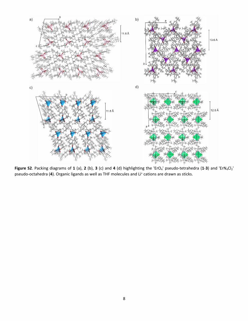
Figure S2. Packing diagrams of 1 (a), 2 (b), 3 (c) and 4 (d) highlighting the 'ErO4' pseudo-tetrahedra (1-3) and 'ErN4Cl2' pseudo-octahedra (4). Organic ligands as well as THF molecules and Li+ cations are drawn as sticks.

9

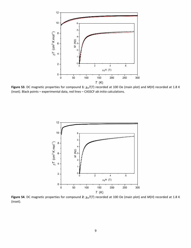
Figure S3. DC magnetic properties for compound 1: χMT(T) recorded at 100 Oe (main plot) and M(H) recorded at 1.8 K (inset). Black points – experimental data, red lines – CASSCF ab initio calculations.

Figure S4. DC magnetic properties for compound 2: χMT(T) recorded at 100 Oe (main plot) and M(H) recorded at 1.8 K (inset).

10

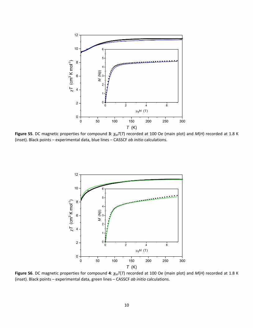
Figure S5. DC magnetic properties for compound 3: χMT(T) recorded at 100 Oe (main plot) and M(H) recorded at 1.8 K (inset). Black points – experimental data, blue lines – CASSCF ab initio calculations.

Figure S6. DC magnetic properties for compound 4: χMT(T) recorded at 100 Oe (main plot) and M(H) recorded at 1.8 K (inset). Black points – experimental data, green lines – CASSCF ab initio calculations.

11

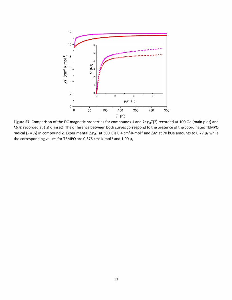
Figure S7. Comparison of the DC magnetic properties for compounds 1 and 2: χMT(T) recorded at 100 Oe (main plot) and M(H) recorded at 1.8 K (inset). The difference between both curves correspond to the presence of the coordinated TEMPO radical (S = ½) in compound 2. Experimental χMT at 300 K is 0.4 cm3Kmol-1 and M at 70 kOe amounts to 0.77 μB while the corresponding values for TEMPO are 0.375 cm3Kmol-1 and 1.00 μB.

12

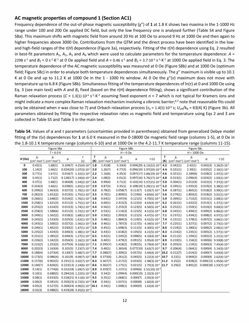
AC magnetic properties of compound 1 (Section AC1)Frequency dependence of the out-of-phase magnetic susceptibility (χ'') of 1 at 1.8 K shows two maxima in the 1-1000 Hz range under 100 and 200 Oe applied DC field, but only the low frequency one is analysed further (Table S4 and Figure S8a). This maximum shifts with magnetic field from around 20 Hz at 100 Oe to around 9 Hz at 1000 Oe and then again to higher frequencies above 3000 Oe. Contributions from the QTM and the direct process have been identified in the low- and high-field ranges of the τ(H) dependence (Figure 3a), respectively. Fitting of the τ(H) dependence using Eq. 2 resulted in best-fit parameters A1, A2, A3 and A4 which were used to calculate parameters for the temperature dependence: A = 2298 s-1 and B2 = 0 s-1K-1 at 0 Oe applied field and A = 0.46 s-1 and B2 = 3.7·10-3 s-1K-1 at 1000 Oe applied field in Eq. 3. The temperature dependence of the AC magnetic susceptibility was measured at 0 Oe (Figure S8b) and at 1000 Oe (optimum field; Figure S8c) in order to analyze both temperature dependences simultaneously. The χ'' maximum is visible up to 10.1 K at 0 Oe and up to 11.2 K at 1000 Oe in the 1 - 1000 Hz window. At 0 Oe the χ''(ν) maximum does not move with temperature up to 6.8 K (Figure S8b). Simultaneous fitting of the temperature dependences of ln(τ) at 0 and 1000 Oe using Eq. 3 (see main text) with A and B2 fixed (based on the τ(H) dependence fitting), shows a significant contribution of the Raman relaxation process (C = 1.3(1)·10-4 s-1K-2 assuming fixed exponent n = 7 which is not typical for Kramers ions and might indicate a more complex Raman relaxation mechanism involving a vibronic barrier;6,7 note that reasonable fits could only be obtained when n was close to 7) and Orbach relaxation process (τ0 = 1.4(5)·10-6 s; Ueff/kB = 63(4) K) (Figure 3b). All parameters obtained by fitting the respective relaxation rates vs magnetic field and temperature using Eqs 2 and 3 are collected in Table S5 and Table 3 in the main text.

Table S4. Values of α and τ parameters (uncertainties provided in parentheses) obtained from generalized Debye model fitting of the τ(ν) dependences for 1 at 6.0 K measured in the 0-18000 Oe magnetic field range (columns 1-5), at 0 Oe in the 1.8-10.1 K temperature range (columns 6-10) and at 1000 Oe in the 4.2-11.7 K temperature range (columns 11-15).

Figure S8a Figure S8b Figure S8cT = 6.0 K H = 0 Oe H = 1000 Oe

H (Oe)χs

(cm3mol-1)χt

(cm3mol-1)α τ

(s)T

(K)χs

(cm3mol-1)χt

(cm3mol-1)α τ (s) T

(K)χs

(cm3mol-1)χt

(cm3mol-1)α τ (s)

0 0.42(1) 1.68(1) 0.104(7) 4.25(4)10-4 1.8 1.41(8) 5.33(4) 0.094(20) 6.13(22)10-4 4.2 0.342(1) 2.42(1) 0.042(3) 3.26(3)10-1

100 1.14(2) 1.66(1) 0.024(20) 1.07(3)10-2 2.0 1.26(7) 4.77(3) 0.096(19) 5.97(20)10-4 4.4 0.331(1) 2.30(1) 0.035(2) 2.16(1)10-1

200 0.77(1) 1.67(1) 0.016(7) 1.32(1)10-2 2.2 1.16(6) 4.35(3) 0.097(17) 5.86(19)10-4 4.6 0.321(1) 2.189(6) 0.028(2) 1.47(1)10-1

300 0.45(1) 1.71(2) 0.128(17) 1.34(4)10-2 2.4 1.08(5) 4.01(2) 0.097(16) 5.76(17)10-4 4.8 0.313(1) 2.096(4) 0.024(2) 1.03(1)10-1

400 0.37(1) 1.68(1) 0.064(8) 1.54(2)10-2 2.6 0.99(4) 3.71(2) 0.102(14) 5.57(15)10-4 5.0 0.304(1) 2.012(4) 0.022(2) 7.37(2)10-2

500 0.324(3) 1.66(1) 0.038(5) 1.65(1)10-2 2.9 0.87(3) 3.35(1) 0.108(10) 5.29(11)10-4 5.2 0.295(1) 1.935(3) 0.019(2) 5.38(2)10-2

600 0.299(2) 1.663(3) 0.027(3) 1.70(1)10-2 3.2 0.78(2) 3.058(7) 0.113(7) 5.03(7)10-4 5.4 0.287(1) 1.865(2) 0.018(2) 3.99(1)10-2

700 0.282(3) 1.652(2) 0.013(5) 1.75(1)10-2 3.5 0.70(1) 2.809(5) 0.119(6) 4.83(6)10-4 5.6 0.279(1) 1.803(2) 0.018(2) 3.01(1)10-2

1000 0.266(1) 1.648(2) 0.014(2) 1.76(1)10-2 3.8 0.64(1) 2.597(4) 0.121(5) 4.70(5)10-4 5.9 0.269(1) 1.713(2) 0.015(1) 2.00(1)10-2

1500 0.258(1) 1.631(3) 0.011(2) 1.75(1)10-2 4.1 0.60(1) 2.415(3) 0.122(4) 4.63(4)10-4 6.2 0.261(1) 1.632(2) 0.013(1) 1.37(1)10-2

2000 0.255(2) 1.614(3) 0.013(3) 1.74(1)10-2 4.4 0.56(1) 2.255(3) 0.123(5) 4.56(5)10-4 6.5 0.252(1) 1.559(1) 0.010(2) 9.60(2)10-3

2500 0.258(3) 1.588(6) 0.011(5) 1.72(1)10-2 4.7 0.53(1) 2.116(3) 0.122(5) 4.51(5)10-4 6.8 0.245(1) 1.494(1) 0.009(2) 6.86(2)10-3

3000 0.249(1) 1.562(2) 0.018(2) 1.68(1)10-2 5.0 0.50(1) 1.993(3) 0.121(5) 4.47(5)10-4 7.1 0.237(1) 1.434(1) 0.008(2) 4.97(1)10-3

3500 0.245(2) 1.533(3) 0.025(3) 1.63(1)10-2 5.3 0.48(1) 1.884(3) 0.119(5) 4.41(5)10-4 7.4 0.231(1) 1.378(1) 0.007(2) 3.66(1)10-3

4000 0.243(1) 1.500(2) 0.027(2) 1.56(1)10-2 5.6 0.46(1) 1.787(3) 0.117(5) 4.34(5)10-4 7.7 0.225(1) 1.327(1) 0.007(2) 2.73(1)10-3

4500 0.240(1) 1.462(2) 0.030(2) 1.47(1)10-2 5.9 0.45(1) 1.698(3) 0.111(5) 4.30(5)10-4 8.0 0.219(2) 1.280(1) 0.006(2) 2.06(1)10-3

5000 0.235(2) 1.424(3) 0.040(3) 1.38(1)10-2 6.2 0.43(1) 1.618(2) 0.105(5) 4.21(5)10-4 8.3 0.214(2) 1.235(1) 0.005(2) 1.57(1)10-3

5500 0.231(1) 1.385(2) 0.044(3) 1.27(1)10-2 6.5 0.42(1) 1.545(2) 0.098(5) 4.10(4)10-4 8.6 0.211(2) 1.194(1) 0.002(2) 1.21(1)10-3

6000 0.226(2) 1.342(3) 0.054(3) 1.16(1)10-2 6.8 0.40(1) 1.479(2) 0.091(5) 3.95(4)10-4 8.9 0.210(5) 1.156(2) 0.000(6) 9.50(8)10-4

7000 0.215(2) 1.253(3) 0.075(4) 9.32(6)10-3 7.1 0.395(7) 1.418(2) 0.082(5) 3.79(4)10-4 9.2 0.203(3) 1.119(1) 0.000(3) 7.45(4)10-4

8000 0.202(3) 1.163(4) 0.101(5) 7.23(7)10-3 7.4 0.40(1) 1.365(4) 0.077(10) 3.63(7)10-4 9.7 0.206(4) 1.064(1) 0.000(4) 5.14(3)10-4

9000 0.188(4) 1.073(4) 0.130(7) 5.48(7)10-3 7.7 0.380(7) 1.309(2) 0.057(5) 3.44(4)10-4 10.2 0.212(7) 1.014(2) 0.000(7) 3.63(4)10-4

10000 0.173(5) 0.986(4) 0.161(9) 4.09(7)10-3 8.0 0.373(6) 1.261(2) 0.045(5) 3.22(3)10-4 10.7 0.22(1) 0.969(2) 0.000(9) 2.62(4)10-4

11000 0.157(6) 0.902(5) 0.191(11) 3.02(7)10-3 8.3 0.367(7) 1.217(2) 0.033(5) 2.98(3)10-4 11.2 0.25(2) 0.928(2) 0.000(13) 1.95(6)10-4

12000 0.140(7) 0.826(5) 0.223(13) 2.24(6)10-3 8.6 0.362(7) 1.175(1) 0.021(5) 2.75(3)10-4 11.7 0.29(2) 0.891(2) 0.000(18) 1.53(7)10-4

13000 0.14(1) 0.774(6) 0.252(18) 1.69(7)10-3 8.9 0.359(7) 1.137(1) 0.009(6) 2.51(10)10-4

14000 0.10(1) 0.688(5) 0.284(16) 1.22(5)10-3 9.2 0.34(2) 1.099(4) 0.000(19) 2.32(3)10-4

15000 0.08(1) 0.633(5) 0.318(21) 9.11(6)10-4 9.5 0.35(1) 1.068(1) 0.000(7) 2.05(3)10-4

16000 0.06(2) 0.581(5) 0.350(23) 6.72(5)10-4 9.8 0.34(1) 1.037(1) 0.000(8) 1.82(4)10-4

17000 0.05(2) 0.527(5) 0.369(24) 4.96(5)10-4 10.1 0.34(1) 1.008(1) 0.000(9) 1.62(4)10-4

18000 0.02(3) 0.488(5) 0.419(28) 3.45(5)10-4

13

Figure S8. In-phase (χ') and out-of-phase (χ'') AC susceptibilities for 1 at 6.0 K measured in the 0-18000 Oe magnetic field range (a), at 0 Oe in the 1.8-10.1 K temperature range (b) and at 1000 Oe in the 4.1-11.7 K temperature range (c). Values of α and τ parameters are gathered in Table S4. The solid lines are the best fits to generalized Debye model.

14

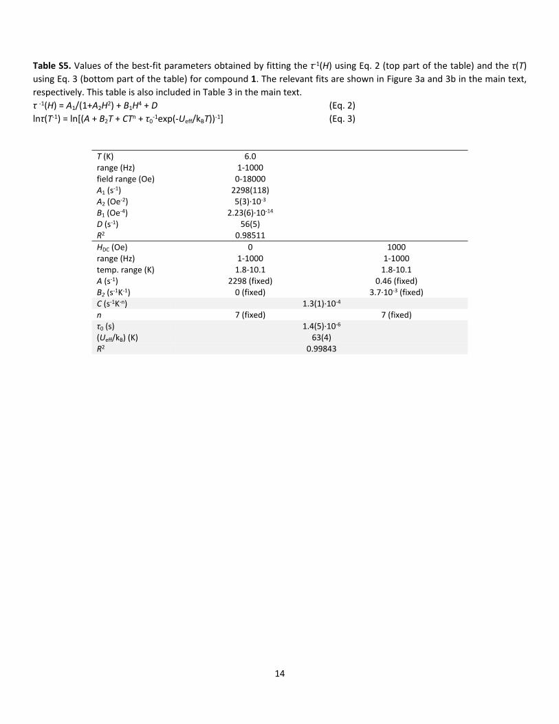
Table S5. Values of the best-fit parameters obtained by fitting the τ-1(H) using Eq. 2 (top part of the table) and the τ(T) using Eq. 3 (bottom part of the table) for compound 1. The relevant fits are shown in Figure 3a and 3b in the main text, respectively. This table is also included in Table 3 in the main text.τ -1(H) = A1/(1+A2H2) + B1H4 + D (Eq. 2)lnτ(T-1) = ln[(A + B2T + CTn + τ0

-1exp(-Ueff/kBT))-1] (Eq. 3)

T (K) 6.0range (Hz) 1-1000field range (Oe) 0-18000A1 (s-1) 2298(118)A2 (Oe-2) 5(3)·10-3

B1 (Oe-4) 2.23(6)·10-14

D (s-1) 56(5)R2 0.98511HDC (Oe) 0 1000range (Hz) 1-1000 1-1000temp. range (K) 1.8-10.1 1.8-10.1A (s-1) 2298 (fixed) 0.46 (fixed)B2 (s-1K-1) 0 (fixed) 3.7·10-3 (fixed)C (s-1K-n) 1.3(1)·10-4

n 7 (fixed) 7 (fixed)τ0 (s) 1.4(5)·10-6

(Ueff/kB) (K) 63(4)R2 0.99843

15

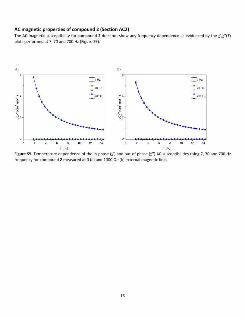
AC magnetic properties of compound 2 (Section AC2)The AC magnetic susceptibility for compound 2 does not show any frequency dependence as evidenced by the χ',χ''(T) plots performed at 7, 70 and 700 Hz (Figure S9).

Figure S9. Temperature dependence of the in-phase (χ') and out-of-phase (χ'') AC susceptibilities using 7, 70 and 700 Hz frequency for compound 2 measured at 0 (a) and 1000 Oe (b) external magnetic field.

16

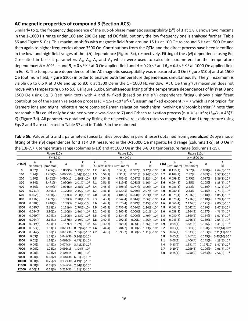
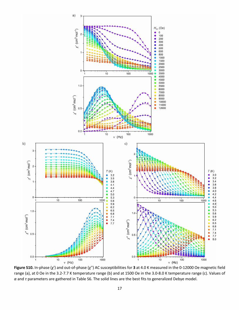
AC magnetic properties of compound 3 (Section AC3)Similarly to 1, the frequency dependence of the out-of-phase magnetic susceptibility (χ'') of 3 at 1.8 K shows two maxima in the 1-1000 Hz range under 100 and 200 Oe applied DC field, but only the low frequency one is analysed further (Table S6 and Figure S10a). This maximum shifts with magnetic field from around 15 Hz at 100 Oe to around 6 Hz at 1500 Oe and then again to higher frequencies above 3500 Oe. Contributions from the QTM and the direct process have been identified in the low- and high-field ranges of the τ(H) dependence (Figure 3c), respectively. Fitting of the τ(H) dependence using Eq. 2 resulted in best-fit parameters A1, A2, A3 and A4 which were used to calculate parameters for the temperature dependence: A = 3096 s-1 and B2 = 0 s-1K-1 at 0 Oe applied field and A = 0.20 s-1 and B2 = 0.3 s-1K-1 at 1000 Oe applied field in Eq. 3. The temperature dependence of the AC magnetic susceptibility was measured at 0 Oe (Figure S10b) and at 1500 Oe (optimum field; Figure S10c) in order to analyze both temperature dependences simultaneously. The χ'' maximum is visible up to 6.5 K at 0 Oe and up to 8.0 K at 1500 Oe in the 1 - 1000 Hz window. At 0 Oe the χ''(ν) maximum does not move with temperature up to 5.8 K (Figure S10b). Simultaneous fitting of the temperature dependences of ln(τ) at 0 and 1500 Oe using Eq. 3 (see main text) with A and B2 fixed (based on the τ(H) dependence fitting), shows a significant contribution of the Raman relaxation process (C = 1.5(1)·10-3 s-1K-2, assuming fixed exponent n = 7 which is not typical for Kramers ions and might indicate a more complex Raman relaxation mechanism involving a vibronic barrier;6,7 note that reasonable fits could only be obtained when n was close to 7) and Orbach relaxation process (τ0 = 7(3)·10-7 s; Ueff/kB = 48(3) K) (Figure 3d). All parameters obtained by fitting the respective relaxation rates vs magnetic field and temperature using Eqs 2 and 3 are collected in Table S7 and in Table 3 in the main text.

Table S6. Values of α and τ parameters (uncertainties provided in parentheses) obtained from generalized Debye model fitting of the τ(ν) dependences for 3 at 4.0 K measured in the 0-16000 Oe magnetic field range (columns 1-5), at 0 Oe in the 1.8-7.7 K temperature range (columns 6-10) and at 1000 Oe in the 3-8.0 K temperature range (columns 1-15).

Figure S10a Figure S10b Figure S10cT = 4.0 K H = 0 Oe H = 1500 Oe

H (Oe)χs

(cm3mol-1)χt

(cm3mol-1)α τ

(s)T

(K)χs

(cm3mol-1)χt

(cm3mol-1)α τ

(s) T (K)χs

(cm3mol-1)χt

(cm3mol-1)α τ

(s)0 0.52(1) 2.456(3) 0.080(5) 3.19(3)10-4 3.2 0.63(2) 5.52(1) 0.092(5) 3.27(4)10-4 3.0 0.116(1) 3.07(4) 0.090(4) 2.64(5)10-1

100 1.74(2) 2.460(6) 0.090(50) 1.44(13)10-2 3.5 0.58(2) 4.91(1) 0.091(6) 3.24(4)10-4 3.2 0.109(1) 2.87(2) 0.089(3) 1.57(1)10-1

200 1.10(1) 2.462(6) 0.090(12) 1.69(3)10-2 3.8 0.54(2) 4.481(6) 0.087(6) 3.22(4)10-4 3.4 0.099(2) 2.75(1) 0.097(3) 9.86(8)10-2

300 0.64(1) 2.471(6) 0.090(6) 2.01(2)10-2 4.1 0.51(2) 4.119(6) 0.083(6) 3.16(4)10-4 3.6 0.094(3) 2.65(1) 0.105(3) 6.35(5)10-2

400 0.36(1) 2.479(6) 0.094(3) 2.28(1)10-2 4.4 0.48(2) 3.808(5) 0.077(6) 3.09(4)10-4 3.8 0.086(3) 2.53(1) 0.110(4) 4.12(3)10-2

500 0.211(4) 2.49(1) 0.120(4) 2.45(2)10-2 4.7 0.46(1) 3.420(5) 0.069(6) 2.97(4)10-4 4.0 0.080(4) 2.43(1) 0.116(4) 2.73(2)10-2

600 0.162(3) 2.480(7) 0.113(3) 2.58(1)10-2 5.0 0.44(1) 3.104(5) 0.058(6) 2.83(4)10-4 4.2 0.075(4) 2.316(8) 0.118(4) 1.85(1)10-2

800 0.116(3) 2.459(7) 0.109(3) 2.70(1)10-2 5.3 0.43(1) 2.842(4) 0.044(6) 2.66(3)10-4 4.4 0.071(4) 2.216(6) 0.118(4) 1.28(1)10-2

1000 0.098(3) 2.440(8) 0.109(3) 2.74(2)10-2 5.6 0.42(1) 2.620(4) 0.029(6) 2.45(3)10-4 4.6 0.066(4) 2.124(6) 0.121(4) 9.00(6)10-3

1500 0.080(4) 2.38(1) 0.111(4) 2.70(2)10-2 5.9 0.41(1) 2.431(4) 0.014(6) 2.24(3)10-4 4.8 0.062(5) 2.042(6) 0.126(4) 6.47(5)10-3

2000 0.084(7) 2.30(2) 0.110(8) 2.60(4)10-2 6.2 0.41(1) 2.267(4) 0.000(6) 2.01(3)10-4 5.0 0.058(5) 1.964(5) 0.127(4) 4.73(4)10-3

2500 0.069(4) 2.24(1) 0.130(5) 2.43(2)10-2 6.5 0.41(2) 2.124(3) 0.000(8) 1.79(4)10-4 5.3 0.050(7) 1.860(6) 0.134(5) 3.07(3)10-3

3000 0.064(4) 2.14(1) 0.137(5) 2.19(2)10-2 6.8 0.40(2) 1.997(3) 0.00(1) 1.55(4)10-4 5.6 0.043(8) 1.766(6) 0.139(6) 2.05(2)10-3

3500 0.049(6) 2.04(1) 0.157(7) 1.89(3)10-2 7.1 0.40(3) 1.885(3) 0.00(1) 1.36(5)10-4 5.9 0.04(1) 1.681(5) 0.146(7) 1.41(2)10-3

4000 0.053(6) 1.91(1) 0.020(33) 8.57(67)10-3 7.4 0.44(4) 1.784(2) 0.00(2) 1.23(7)10-4 6.2 0.03(1) 1.603(5) 0.150(7) 9.92(14)10-4

4500 0.044(7) 1.80(1) 0.020(36) 7.05(43)10-3 7.7 0.47(5) 1.693(2) 0.00(2) 1.11(9)10-4 6.5 0.04(1) 1.533(5) 0.153(8) 7.21(11)10-4

5000 0.03(1) 1.67(1) 0.049(36) 5.86(35)10-3 6.8 0.05(1) 1.467(5) 0.149(9) 5.43(10)10-4

5500 0.02(1) 1.56(2) 0.061(24) 4.47(18)10-3 7.1 0.08(2) 1.406(4) 0.143(9) 4.23(9)10-4

6000 0.00(1) 1.45(2) 0.074(24) 3.41(13)10-3 7.4 0.13(2) 1.351(4) 0.127(10) 3.47(8)10-4

7000 0.00(2) 1.23(2) 0.096(15) 1.94(5)10-3 7.7 0.19(2) 1.299(3) 0.106(9) 2.96(6)10-4

8000 0.00(3) 1.03(2) 0.104(15) 1.10(3)10-3 8.0 0.25(1) 1.250(2) 0.083(8) 2.56(5)10-4

9000 0.00(4) 0.88(2) 0.107(38) 6.51(33)10-4

10000 0.00(6) 0.75(2) 0.133(30) 4.19(16)10-4

11000 0.00(8) 0.65(2) 0.149(54) 2.84(22)10-4

12000 0.00(11) 0.58(3) 0.221(31) 1.91(12)10-4

17

Figure S10. In-phase (χ') and out-of-phase (χ'') AC susceptibilities for 3 at 4.0 K measured in the 0-12000 Oe magnetic field range (a), at 0 Oe in the 3.2-7.7 K temperature range (b) and at 1500 Oe in the 3.0-8.0 K temperature range (c). Values of α and τ parameters are gathered in Table S6. The solid lines are the best fits to generalized Debye model.

18

Table S7. Values of the best-fit parameters obtained by fitting the τ-1(H) using Eq. 2 (top part of the table) and the τ(T) using Eq. 3 (bottom part of the table) for compound 3. The relevant fits are shown in Figure 3c and 3d in the main text, respectively. This table is also included in Table 3 in the main text.τ -1(H) = A1/(1+A2H2) + B1H4 + D (Eq. 2)lnτ(T-1) = ln[(A + B2T + CTn + τ0

-1exp(-Ueff/kBT))-1] (Eq. 3)

T (K) 4.0range (Hz) 1-1000field range (Oe) 0-12000A1 (s-1) 3096(104)A2 (Oe-2) 7(3)·10-3

B1 (Oe-4) 2.36(4)·10-13

D (s-1) 34(4)R2 0.99569HDC (Oe) 0 1500range (Hz) 1-1000 1-1000temp. range (K) 3.2-7.7 3.0-8.0A (s-1) 3096 (fixed) 0.20 (fixed)B2 (s-1K-1) 0 (fixed) 3.0·10-1 (fixed)C (s-1K-n) 1.5(1)·10-3

n 7 (fixed) 7 (fixed)τ0 (s) 7(3)·10-7

(Ueff/kB) (K) 48(3)R2 0.99818

19

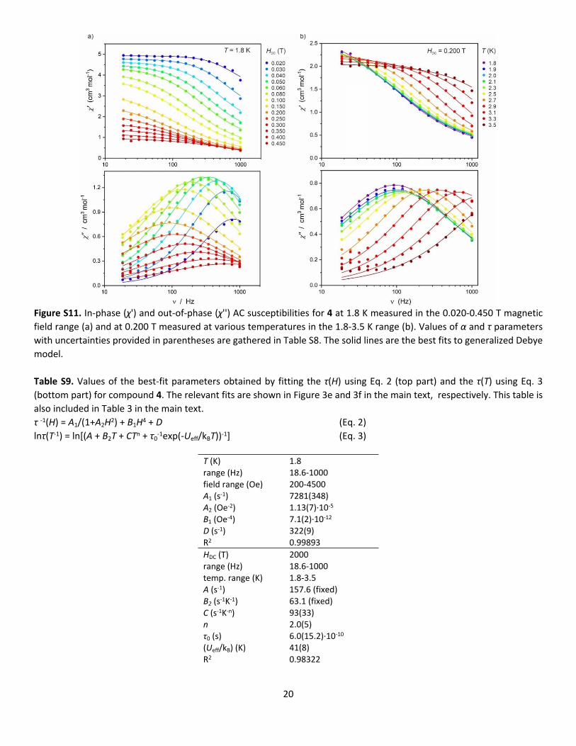
AC magnetic properties of compound 4 (Section AC4)Frequency dependence of the out-of-phase magnetic susceptibility (χ'') of 4 shows a single maximum in the 18.6-1000 Hz range under small applied DC field (T = 1.8 K; Table S8 and Figure S11a). This χ'' maximum shifts with the magnetic field from around 850 Hz at 200 Oe to around 100 Hz at 2000 Oe (optimum field) and then again to higher frequencies in the 2000-4500 Oe range. Contributions from the QTM and the direct process have been identified in the low- and high-field ranges of the τ(H) dependence (Figure 3e), respectively. Fitting of the τ(H) dependence using Eq. 2 resulted in best-fit parameters A1, A2, A3 and A4 which were used to calculate parameters: A = 157.6 s-1 and B2 = 63.1 s-1K-1 in Eq. 3. The temperature dependence of the AC magnetic susceptibility was measured at the optimum DC field of 2000 Oe in order to analyze the temperature dependence of the relaxation process in a possibly wide temperature range. The χ'' maximum is visible up to 3.3 K in the 18.6 - 1000 Hz window and shows larger thermal shift above 2.5 K (Figure S11b and Table S8). Fitting of the temperature dependence of ln(τ) using Eq. 3 (see main text) with A and B2 fixed based on the results of τ(H) dependence fitting, shows a significant contribution of the phonon bottle-neck process (C = 93(33) s-1K-2, n = 2.0(5)) and Orbach relaxation process (τ0 = 6.0(15.2)·10-10 s; Ueff/kB = 41(8) K) (Figure 3f). All parameters obtained by fitting the respective relaxation rates vs magnetic field and temperature using Eqs 2 and 3 are collected in Table S9 and in Table 3 in the main text.

Table S8. Values of α and τ parameters with uncertainties provided in parentheses obtained from generalized Debye model fitting of the τ(ν) dependences for 4 at 1.8 K in the 0.020-0.450 T magnetic field range (columns 1-5) and at 0.200 T measured at various temperatures in the 1.8-3.5 K range (columns 6-10).

Figure S11a Figure S11bT = 1.8 K H = 2000 Oe

H(Oe)

χs

(cm3mol-1)χt

(cm3mol-1)α τ

(s)T

(K)χs

(cm3mol-1)χt

(cm3mol-1)α τ

(s)200 3.26(9) 4.93(2) 0.012(30) 1.97(14)·10-4 1.8 0.21(1) 2.80(2) 0.306(7) 16.9(3)·10-4

300 2.19(6) 4.78 (2) 0.069(16) 2.52(9)·10-4 1.9 0.21(2) 2.73(2) 0.319(9) 15.8(3)·10-4

400 1.48(4) 4.65(1) 0.132(9) 3.40(7)·10-4 2.0 0.23(2) 2.67(2) 0.310(10) 15.0(3)·10-4

500 1.05(3) 4.54(1) 0.172(7) 4.46(7)·10-4 2.1 0.23(1) 2.70(1) 0.318(6) 15.0(2)·10-4

600 0.78(3) 4.44(1) 0.200(6) 5.73(7)·10-4 2.3 0.24(2) 2.60(2) 0.296(8) 12.7(2)·10-4

800 0.47(2) 4.22(2) 0.241(6) 8.27(9)·10-4 2.5 0.26(2) 2.51(1) 0.261(7) 10.0(1)·10-4

1000 0.30(2) 4.03(2) 0.283(5) 10.9(1)·10-4 2.7 0.28(2) 2.36(1) 0.211(9) 6.71(11)·10-4

1500 0.21(1) 3.37(2) 0.310(5) 15.6(2)·10-4 2.9 0.25(4) 2.28(1) 0.194(15) 4.12(14)·10-4

2000 0.19(2) 2.77(3) 0.319(10) 16.9(4)·10-4 3.1 0.22(7) 2.20(2) 0.191(21) 2.36(15)·10-4

2500 0.18(1) 2.25(2) 0.308(8) 14.5(2)·10-4 3.3 0.19(17) 2.13 (2) 0.206(36) 1.28(21)·10-4

3000 0.19(2) 1.74(2) 0.260(14) 10.0(3)·10-4 3.5 -0.05(50) 2.06(2) 0.263(54) 0.54(25)·10-4

3500 0.15(2) 1.43(1) 0.277(17) 6.94(25)·10-4

4000 0.022(82) 1.22(3) 0.371(46) 4.08(63)·10-4

4500 -0.011(116) 1.00(3) 0.385(60) 2.41(68)·10-4

20

Figure S11. In-phase (χ') and out-of-phase (χ'') AC susceptibilities for 4 at 1.8 K measured in the 0.020-0.450 T magnetic field range (a) and at 0.200 T measured at various temperatures in the 1.8-3.5 K range (b). Values of α and τ parameters with uncertainties provided in parentheses are gathered in Table S8. The solid lines are the best fits to generalized Debye model.

Table S9. Values of the best-fit parameters obtained by fitting the τ(H) using Eq. 2 (top part) and the τ(T) using Eq. 3 (bottom part) for compound 4. The relevant fits are shown in Figure 3e and 3f in the main text, respectively. This table is also included in Table 3 in the main text.τ -1(H) = A1/(1+A2H2) + B1H4 + D (Eq. 2)lnτ(T-1) = ln[(A + B2T + CTn + τ0

-1exp(-Ueff/kBT))-1] (Eq. 3)

T (K) 1.8range (Hz) 18.6-1000field range (Oe) 200-4500A1 (s-1) 7281(348)A2 (Oe-2) 1.13(7)·10-5

B1 (Oe-4) 7.1(2)·10-12

D (s-1) 322(9)R2 0.99893HDC (T) 2000range (Hz) 18.6-1000temp. range (K) 1.8-3.5A (s-1) 157.6 (fixed)B2 (s-1K-1) 63.1 (fixed)C (s-1K-n) 93(33)n 2.0(5)τ0 (s) 6.0(15.2)·10-10

(Ueff/kB) (K) 41(8)R2 0.98322

21

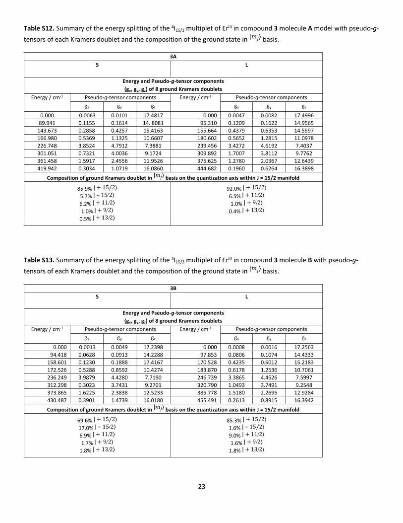
Ab initio calculationsAb initio calculations were carried out using the OpenMolcas quantum chemistry software package,8 and were performed on experimental geometries taken from the single crystal X-ray diffraction analysis. For 3 two non-equivalent molecules denoted as 3A and 3B were considered, while for 1 and 4 only one molecule was taken for analysis. The fragments of crystal structure employed for analysis together with calculated main quantization axes (z) are presented in Figure 4. Two models with different basis sets were used: S - small with VDZP basis function quality for ErIII central ion and VDZ for other atoms and L – large with VTZP basis for ErIII and VDZP for atoms in the first coordination sphere together with Li ions. Table S10 contains contractions and labels of basis sets S and L for all atoms. The performed calculations were of CASSCF/RASSI/SINGLE_ANISO type.9 Scalar relativistic effects were taken into account by employing second order DKH (Douglas-Kroll-Hess) Hamiltonian and relativistic basis sets of an ANO-RCC type. In order to save disk space, Cholesky decomposition of ERI-s (electron repulsion integrals) was used with the 1.0·10-8 threshold. In the first step, a state average multi-configurational self-consistent field (SA-CASSCF) calculation for 35 quartets and 112 doublets rising from different ErIII configurations was carried out. The active space was composed out of seven f-orbitals with eleven active valence electrons – CAS(11in7). In the next step, all quartets and doublets optimized as spin-free states in CASSCF step were mixed by the spin-orbit coupling within RASSI (Restricted Active Space State Interaction Program) using mean-field spin-orbit (SO) integrals (AMFI) resulting in 364 spin-orbit states. In the final step, a SINGLE_ANISO module was used to decompose the spin-orbit states into states with a definite projection of the total momentum on the located quantization axis and to calculate crystal-field parameters of the Zero Field Splitting (ZFS) Hamiltonian within the manifold of J = 15/2 together with three components of the pseudo-g-tensor for eight ground Kramers doublets.10 The obtained energy splitting of the J = 15/2 manifold, together with the gx, gy, gz components of the pseudo-g-tensors within the basis of each doublet (

and decomposition of the ground state into states with a definite angular momentum on quantization axis are �̃� = 1/2)

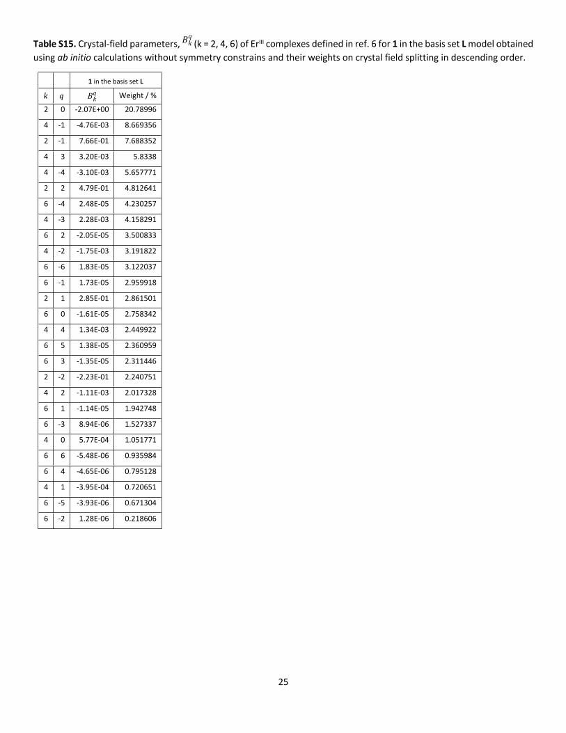
presented in Tables S11-S14. All 27 crystal-field parameters of rank k = 2, 4 and 6 were gathered in Tables S15-S17 together with their weights on the crystal field splitting. Magnetic transition moments between states for 1, 3 and 4 are visualized in Figure 4 in the article. Comparison of the calculated M(H) and χT(T) dependencies (solid lines) with experimental ones (points) can be found in Figures S3, S5 and S6. The agreement between the calculated and experimental data is satisfactory.

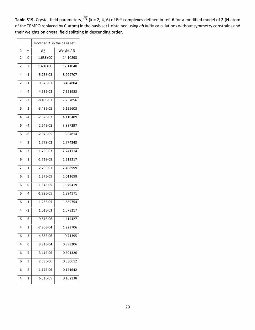
Attempts to calculate the energy diagram and magnetic properties of 2 were unsuccessful due to the additional spin on the TEMPO ligand. However, in order to better understand the crystal field in 2, we have replaced the N atom in TEMPO with the C atom so that the TEMPO has lost its radical character and the calculations were possible for such a modified model of 2 (Table S18 and S19).

22

Table S10. Description and contractions of the basis sets (two models: S - small, L - large) employed in ab initio calculations of the ErIII crystal field in Er_ttbp (compound 1), Er_bht_1 (compound 3), Er_bht_2 (compound 3) and Er_n3ncl2 Er_ttbp (compound 4).

Table S11. Summary of the energy splitting of the 4I15/2 multiplet of ErIII in compound 1 with pseudo-g-tensors of each Kramers doublet and the composition of the ground state in basis.|𝑚𝐽⟩

Compound 1S L

Energy and Pseudo-g-tensor components(gx, gy, gz) of 8 ground Kramers doublets

Pseudo-g-tensor components Pseudo-g-tensor componentsEnergy / cm-1

gx gy gz

Energy / cm-1

gx gy gz

0.000 0.0166 0.0261 17.6511 0.000 0.0070 0.0129 17.654899.740 0.2645 0.6156 14.2647 104.431 0.0670 0.1459 14.8648

140.763 0.5799 1.1535 15.9697 156.372 0.5801 1.3121 15.2402162.438 1.2964 3.3779 10.0513 176.619 0.6328 2.5562 10.1457226.866 7.7119 6.3032 2.6093 241.634 7.0440 6.5546 2.9839317.568 2.1591 4.0788 8.2183 330.470 0.9440 4.0624 8.7756371.244 2.3020 3.6540 11.2772 388.376 2.1676 2.7734 11.3834423.222 0.4566 1.6293 16.2343 439.286 0.4359 1.5891 15.8730

Composition of ground Kramers doublet in the basis on the quantization axis of the ground doublet within J = |𝑚𝐽⟩

15/2 manifold

90.0% | + 15/2⟩5.9% | ‒ 15 2⟩2.0% | + 11 2⟩1.3% | + 9 2⟩0.3% | + 7 2⟩

0.2% | + 13 2⟩

65.4% | + 15/2⟩30.3% | ‒ 15/2⟩1.8% | + 11 2⟩0.8% | ‒ 11 2⟩0.8% | + 9 2⟩0.4% | ‒ 9 2⟩

Basis set “S” Basis set “L”

Er.ANO-RCC-VDZP 7S6P4D2F1G Er.ANO-RCC-VTZP 8S7P5D3F2G1H

Li.ANO-RCC-VDZ 3S2P Li.ANO-RCC-VDZP 3S2P1D

Cl.ANO-RCC-VDZ 4S3P Cl.ANO-RCC-VDZP 4S3P1D

Si.ANO-RCC_VDZ 4S3P Si.ANO-RCC_VDZ 4S3P

N.ANO-RCC-VDZ 3S2P N.ANO-RCC-VDZP 3S2P1D

O.ANO-RCC-VDZ 3S2PO.ANO-RCC-VDZ 3S2P (distant atoms in Er_n3ncl2)O.ANO-RCC-VDZP 3S2P1D (first coordination sphere in Er_bht)

C.ANO-RCC-VDZ 3S2P C.ANO-RCC-VDZ 3S2P

H.ANO-RCC-VDZ 2S H.ANO-RCC-VDZ 2S

23

Table S12. Summary of the energy splitting of the 4I15/2 multiplet of ErIII in compound 3 molecule A model with pseudo-g-tensors of each Kramers doublet and the composition of the ground state in basis.|𝑚𝐽⟩

3AS L

Energy and Pseudo-g-tensor components(gx, gy, gz) of 8 ground Kramers doublets

Pseudo-g-tensor components Pseudo-g-tensor componentsEnergy / cm-1

gx gy gz

Energy / cm-1

gx gy gz

0.000 0.0063 0.0101 17.4817 0.000 0.0047 0.0082 17.499689.941 0.1155 0.1614 14. 8081 95.310 0.1209 0.1622 14.9565

143.673 0.2858 0.4257 15.4163 155.664 0.4379 0.6353 14.5597166.980 0.5369 1.1325 10.6607 180.602 0.5652 1.2815 11.0978226.748 3.8524 4.7912 7.3881 239.456 3.4272 4.6192 7.4037301.051 0.7321 4.0036 9.1724 309.892 1.7007 3.8112 9.7762361.458 1.5917 2.4556 11.9526 375.625 1.2780 2.0367 12.6439419.942 0.3034 1.0719 16.0860 444.682 0.1960 0.6264 16.3898

Composition of ground Kramers doublet in basis on the quantization axis within J = 15/2 manifold|𝑚𝐽⟩

85.9% | + 15/2⟩5.7% | ‒ 15 2⟩6.2% | + 11 2⟩1.0% | + 9 2⟩

0.5% | + 13 2⟩

92.0% | + 15/2⟩6.5% | + 11 2⟩1.0% | + 9 2⟩

0.4% | + 13 2⟩

Table S13. Summary of the energy splitting of the 4I15/2 multiplet of ErIII in compound 3 molecule B with pseudo-g-tensors of each Kramers doublet and the composition of the ground state in basis.|𝑚𝐽⟩

3BS L

Energy and Pseudo-g-tensor components(gx, gy, gz) of 8 ground Kramers doublets

Pseudo-g-tensor components Pseudo-g-tensor componentsEnergy / cm-1

gx gy gz

Energy / cm-1

gx gy gz

0.000 0.0013 0.0049 17.2398 0.000 0.0008 0.0016 17.256394.418 0.0628 0.0913 14.2288 97.853 0.0806 0.1074 14.4333

158.601 0.1230 0.1888 17.4167 170.528 0.4235 0.6012 15.2183172.526 0.5288 0.8592 10.4274 183.870 0.6178 1.2536 10.7061236.249 3.9879 4.4280 7.7190 246.739 3.3865 4.4526 7.5997312.298 0.3023 3.7431 9.2701 320.790 1.0493 3.7491 9.2548373.865 1.6225 2.3838 12.5233 385.778 1.5180 2.2695 12.9284430.487 0.3901 1.4739 16.0180 455.491 0.2613 0.8915 16.3942Composition of ground Kramers doublet in basis on the quantization axis within J = 15/2 manifold|𝑚𝐽⟩

69.6% | + 15/2⟩17.0% | ‒ 15 2⟩6.9% | + 11 2⟩1.7% | + 9 2⟩

1.8% | + 13 2⟩

85.3% | + 15/2⟩1.6% | ‒ 15/2⟩9.0% | + 11 2⟩1.6% | + 9 2⟩

1.8% | + 13 2⟩

24

Table S14. Summary of the energy splitting of the 4I15/2 multiplet of ErIII in compound 4 with pseudo-g-tensors of each Kramers doublet and the composition of the ground state in basis.|𝑚𝐽⟩

Compound 4S L

Energy and Pseudo-g-tensor components(gx, gy, gz) of 8 ground Kramers doublets

Pseudo-g-tensor components Pseudo-g-tensor componentsEnergy / cm-1

gx gy gz

Energy / cm-1

gx gy gz

0.000 0.0358 0.0824 16.4810 0.000 0.0480 0.1031 16.444039.535 0.0067 0.1101 12.8726 30.556 0.0296 0.1454 12.7906

101.488 2.3153 2.3826 9.0310 89.274 1.7998 1.9254 8.9212155.009 4.0910 5.7441 8.3308 140.862 4.7443 5.2939 8.8112217.760 0.0350 2.3700 13.5905 223.688 2.2751 5.3122 8.9437256.080 0.8858 1.8978 13.8751 249.360 1.7824 5.1874 10.5539308.850 0.0672 0.8419 16.5299 280.533 0.0887 0.9437 16.3007338.370 0.0858 0.8477 16.7534 331.665 0.1312 0.4231 17.1844Composition of ground Kramers doublet in basis on the quantization axis within J = 15/2 manifold|𝑚𝐽⟩

40.5% | + 15/2⟩23.6% | ‒ 15 2⟩12.1% | + 13 2⟩7.3% | + 11 2⟩7.0% | ‒ 13 2⟩4.1% | ‒ 11 2⟩2.6% | + 9 2⟩1.8% | ‒ 9 2⟩

31.5% | + 15/2⟩31.5% | ‒ 15 2⟩9.9% | + 13 2⟩9.9% | ‒ 13 2⟩6.1% | ‒ 11 2⟩5.8% | ‒ 11 2⟩2.3% | ‒ 9 2⟩1.8% | + 9 2⟩

25

Table S15. Crystal-field parameters, (k = 2, 4, 6) of ErIII complexes defined in ref. 6 for 1 in the basis set L model obtained 𝐵𝑞𝑘

using ab initio calculations without symmetry constrains and their weights on crystal field splitting in descending order.

1 in the basis set L

𝑘 𝑞 𝐵𝑞𝑘 Weight / %

2 0 -2.07E+00 20.78996

4 -1 -4.76E-03 8.669356

2 -1 7.66E-01 7.688352

4 3 3.20E-03 5.8338

4 -4 -3.10E-03 5.657771

2 2 4.79E-01 4.812641

6 -4 2.48E-05 4.230257

4 -3 2.28E-03 4.158291

6 2 -2.05E-05 3.500833

4 -2 -1.75E-03 3.191822

6 -6 1.83E-05 3.122037

6 -1 1.73E-05 2.959918

2 1 2.85E-01 2.861501

6 0 -1.61E-05 2.758342

4 4 1.34E-03 2.449922

6 5 1.38E-05 2.360959

6 3 -1.35E-05 2.311446

2 -2 -2.23E-01 2.240751

4 2 -1.11E-03 2.017328

6 1 -1.14E-05 1.942748

6 -3 8.94E-06 1.527337

4 0 5.77E-04 1.051771

6 6 -5.48E-06 0.935984

6 4 -4.65E-06 0.795128

4 1 -3.95E-04 0.720651

6 -5 -3.93E-06 0.671304

6 -2 1.28E-06 0.218606

26

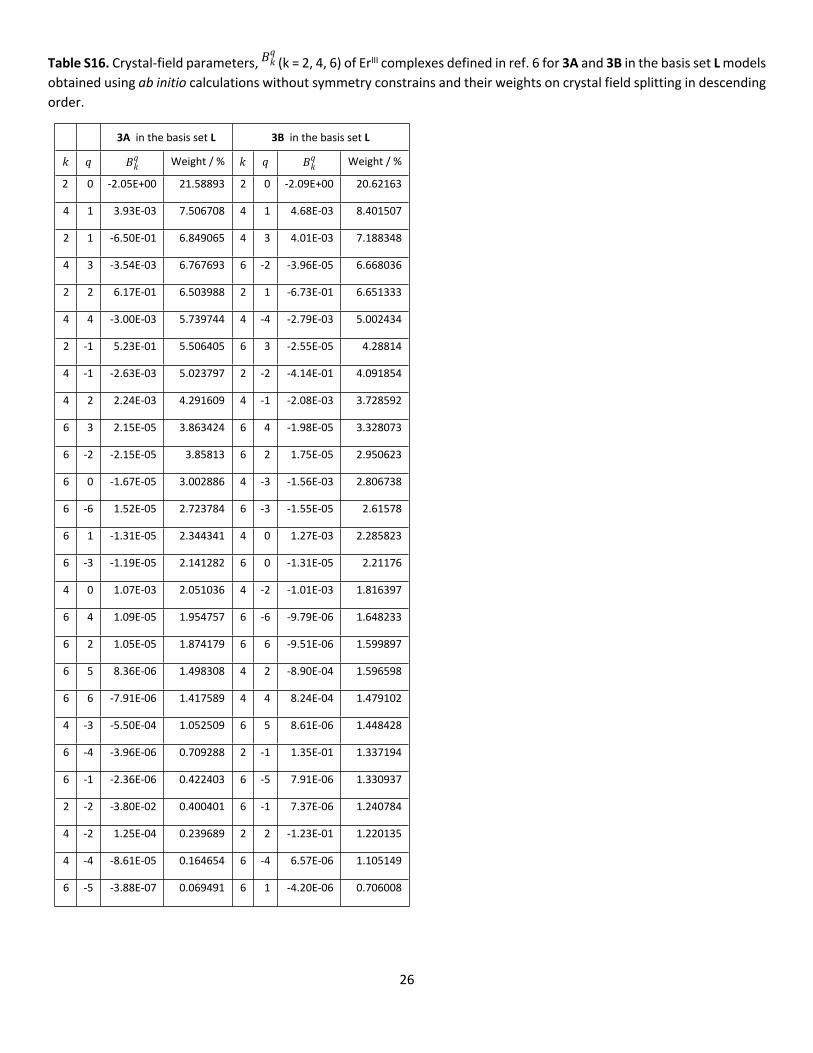
Table S16. Crystal-field parameters, (k = 2, 4, 6) of ErIII complexes defined in ref. 6 for 3A and 3B in the basis set L models 𝐵𝑞𝑘

obtained using ab initio calculations without symmetry constrains and their weights on crystal field splitting in descending order.

3A in the basis set L 3B in the basis set L

𝑘 𝑞 𝐵𝑞𝑘 Weight / % 𝑘 𝑞 𝐵𝑞

𝑘 Weight / %

2 0 -2.05E+00 21.58893 2 0 -2.09E+00 20.62163

4 1 3.93E-03 7.506708 4 1 4.68E-03 8.401507

2 1 -6.50E-01 6.849065 4 3 4.01E-03 7.188348

4 3 -3.54E-03 6.767693 6 -2 -3.96E-05 6.668036

2 2 6.17E-01 6.503988 2 1 -6.73E-01 6.651333

4 4 -3.00E-03 5.739744 4 -4 -2.79E-03 5.002434

2 -1 5.23E-01 5.506405 6 3 -2.55E-05 4.28814

4 -1 -2.63E-03 5.023797 2 -2 -4.14E-01 4.091854

4 2 2.24E-03 4.291609 4 -1 -2.08E-03 3.728592

6 3 2.15E-05 3.863424 6 4 -1.98E-05 3.328073

6 -2 -2.15E-05 3.85813 6 2 1.75E-05 2.950623

6 0 -1.67E-05 3.002886 4 -3 -1.56E-03 2.806738

6 -6 1.52E-05 2.723784 6 -3 -1.55E-05 2.61578

6 1 -1.31E-05 2.344341 4 0 1.27E-03 2.285823

6 -3 -1.19E-05 2.141282 6 0 -1.31E-05 2.21176

4 0 1.07E-03 2.051036 4 -2 -1.01E-03 1.816397

6 4 1.09E-05 1.954757 6 -6 -9.79E-06 1.648233

6 2 1.05E-05 1.874179 6 6 -9.51E-06 1.599897

6 5 8.36E-06 1.498308 4 2 -8.90E-04 1.596598

6 6 -7.91E-06 1.417589 4 4 8.24E-04 1.479102

4 -3 -5.50E-04 1.052509 6 5 8.61E-06 1.448428

6 -4 -3.96E-06 0.709288 2 -1 1.35E-01 1.337194

6 -1 -2.36E-06 0.422403 6 -5 7.91E-06 1.330937

2 -2 -3.80E-02 0.400401 6 -1 7.37E-06 1.240784

4 -2 1.25E-04 0.239689 2 2 -1.23E-01 1.220135

4 -4 -8.61E-05 0.164654 6 -4 6.57E-06 1.105149

6 -5 -3.88E-07 0.069491 6 1 -4.20E-06 0.706008

27

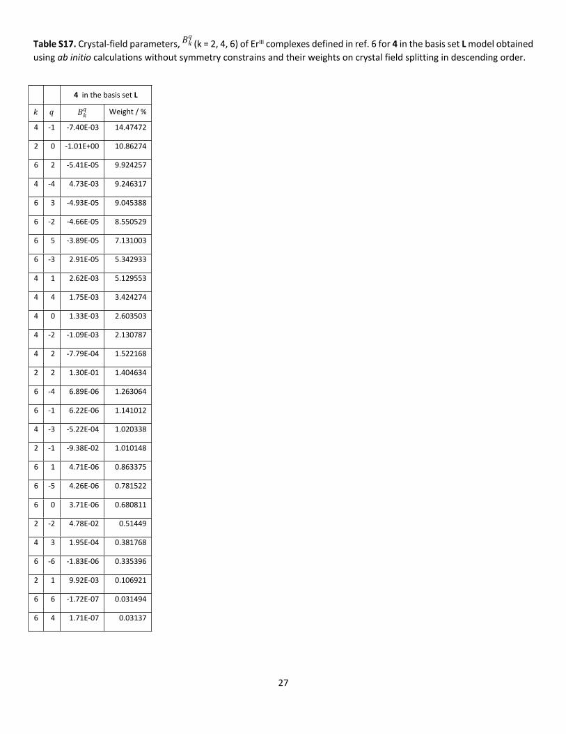
Table S17. Crystal-field parameters, (k = 2, 4, 6) of ErIII complexes defined in ref. 6 for 4 in the basis set L model obtained 𝐵𝑞𝑘

using ab initio calculations without symmetry constrains and their weights on crystal field splitting in descending order.

4 in the basis set L

𝑘 𝑞 𝐵𝑞𝑘 Weight / %

4 -1 -7.40E-03 14.47472

2 0 -1.01E+00 10.86274

6 2 -5.41E-05 9.924257

4 -4 4.73E-03 9.246317

6 3 -4.93E-05 9.045388

6 -2 -4.66E-05 8.550529

6 5 -3.89E-05 7.131003

6 -3 2.91E-05 5.342933

4 1 2.62E-03 5.129553

4 4 1.75E-03 3.424274

4 0 1.33E-03 2.603503

4 -2 -1.09E-03 2.130787

4 2 -7.79E-04 1.522168

2 2 1.30E-01 1.404634

6 -4 6.89E-06 1.263064

6 -1 6.22E-06 1.141012

4 -3 -5.22E-04 1.020338

2 -1 -9.38E-02 1.010148

6 1 4.71E-06 0.863375

6 -5 4.26E-06 0.781522

6 0 3.71E-06 0.680811

2 -2 4.78E-02 0.51449

4 3 1.95E-04 0.381768

6 -6 -1.83E-06 0.335396

2 1 9.92E-03 0.106921

6 6 -1.72E-07 0.031494

6 4 1.71E-07 0.03137

28

Table S18. Summary of the energy splitting of the 4I15/2 multiplet of ErIII in a modified model of compound 2 (N-atom of the TEMPO replaced by C-atom) with pseudo-g-tensors of each Kramers doublet and the composition of the ground state in basis.|𝑚𝐽⟩

Modified model of compound 2S L

Energy and Pseudo-g-tensor components(gx, gy, gz) of 8 ground Kramers doublets

Pseudo-g-tensor components Pseudo-g-tensor componentsEnergy / cm-1

gx gy gz

Energy / cm-1

gx gy gz

0.000 0.0363 0.1047 16.5251 0.000 0.0362 0.0611 17.283328.678 0.0286 0.1235 15.7704 43.882 0.0359 0.0905 16.481493.649 0.2365 0.3003 15.4267 101.200 0.3429 0.4377 14.8384

120.374 1.1035 1.3877 10.4748 138.069 1.1025 1.3779 11.0316170.974 3.9208 4.8550 6.9869 185.379 4.0245 4.9822 6.4596241.144 0.5377 3.3337 8.1177 257.340 0.2519 3.1021 8.4893285.345 1.2909 4.4076 11.8418 308.092 1.1303 3.5089 12.5626426.301 0.0306 0.0633 17.5141 459.700 0.0281 0.0602 17.5406

Composition of ground Kramers doublet in the basis on the quantization axis of the ground doublet within J = |𝑚𝐽⟩

15/2 manifold

69.4% | + 15/2⟩14.1% | + 13 2⟩7.0% | + 11 2⟩6.6% | + 9 2⟩1.6 % | + 7 2⟩0.5% | ‒ 15 2⟩

85.1% | + 15/2⟩4.1% | ‒ 15 2⟩4.1% | + 11 2⟩2.9% | + 9 2⟩

1.8% | + 13 2⟩1.1% | + 7 2⟩

29

Table S19. Crystal-field parameters, (k = 2, 4, 6) of ErIII complexes defined in ref. 6 for a modified model of 2 (N-atom 𝐵𝑞𝑘

of the TEMPO replaced by C-atom) in the basis set L obtained using ab initio calculations without symmetry constrains and their weights on crystal field splitting in descending order.

modified 2 in the basis set L

𝑘 𝑞 𝐵𝑞𝑘 Weight / %

2 0 -1.63E+00 14.10893

2 2 1.40E+00 12.11048

4 -1 -5.73E-03 8.999707

2 -1 9.82E-01 8.494804

4 4 4.68E-03 7.351983

2 -2 -8.40E-01 7.267856

6 2 -3.48E-05 5.125603

4 -4 -2.62E-03 4.110489

6 -4 2.64E-05 3.887397

6 -6 -2.07E-05 3.04814

4 3 1.77E-03 2.774343

4 -3 1.75E-03 2.741114

6 1 -1.71E-05 2.513217

2 1 2.79E-01 2.408999

6 5 1.37E-05 2.011658

6 0 -1.34E-05 1.979419

6 4 -1.29E-05 1.894171

6 -1 1.25E-05 1.839754

4 -2 1.01E-03 1.578217

6 6 9.61E-06 1.414427

4 2 -7.80E-04 1.223706

6 -3 4.85E-06 0.71395

4 0 3.81E-04 0.598206

6 -5 3.41E-06 0.501326

6 3 2.59E-06 0.380612

6 -2 1.17E-06 0.171642

4 1 6.51E-05 0.102138

30

References1. C. C. Cummins, R. R. Schrock, W. M. Davis, Inorg. Chem. 1994, 33, 1448–14572. F. Yuan, J. Yang, L. Xiong, J. Organomet. Chem. 2006, 691, 2534-25393. G. M. Sheldrick, Acta Crystallogr. C, 2015, 71, 3–84. O. V Dolomanov, L. J. Bourhis, R. J. Gildea, J. A. K. Howard and H. Puschmann, J. Appl. Crystallogr., 2009, 42, 339–3415. M. Arczyński, J. Stanek, B. Sieklucka, K. R. Dunbar and D. Pinkowicz, J. Am. Chem. Soc., 2019, 141, 19067–190776. L. Gu, R. Wu, Phys. Rev. B, 2021, 103, 0144017. K. N. Shrivastava, Phys. Stat. Sol. B, 1983, 117, 437-4588. I. F. Galvam, M. Vacher, A. Alavi, C. Angeli, F. Aquilante, J. Autschbach, J. J. Bao, S. I. Bokarev, N. A. Bogdanov, R. K. Carlson, L. F. Chibotaru, J. Creutzberg, N. Dattani, M. G. Delcey, S. S. Dong, A. Dreuw, L. Freitag, L. M. Frutos, L. Gagliardi, F. Gendron, A. Giussani, L. Gonzalez, G. Grell, M. Guo, C. E. Hoyer, M. Johansson, S. Keller, S. Knecht, G. Kovacevic, E. Kallman, G. L. Manni, M. Lundberg, Y. Ma, S. Mai, J. P. Malhado, P. A. Malmqvist, P. Marquetand, S. A. Mewes, J. Norell, M. Olivucci, M. Oppel, Q. M. Phung, K. Perloot, F. Plasser, M. Reiher, A. M. Sand, I. Schapiro, P. Sharma, C. J. Stein, L. K. Sorensen, D. G. Truhlar, M. Ugandi, L. Ungur, A. Valentini, S. Vancoillie, V. Veryazov, O. Weser, T. A. Wesołowski, P.-O. Widmark, S. Wouters, A. Zech, J. P. Zobel, R. Lindh, J. Chem. Theory Comput. 2019, 15, 5925–59649. L. F. Chibotaru, L. Ungur, J. Chem. Phys. 2012, 137, 06411210. L. Ungur, L. F. Chibotaru, Chem. Eur. J. 2017, 23, 3708–3718