electron beam dynamics with and without compton back scattering
TRANSCRIPT

HAL Id: tel-00920424https://tel.archives-ouvertes.fr/tel-00920424
Submitted on 18 Dec 2013
HAL is a multi-disciplinary open accessarchive for the deposit and dissemination of sci-entific research documents, whether they are pub-lished or not. The documents may come fromteaching and research institutions in France orabroad, or from public or private research centers.
L’archive ouverte pluridisciplinaire HAL, estdestinée au dépôt et à la diffusion de documentsscientifiques de niveau recherche, publiés ou non,émanant des établissements d’enseignement et derecherche français ou étrangers, des laboratoirespublics ou privés.
Electron beam dynamics with and without Comptonback scattering
Illya Drebot
To cite this version:Illya Drebot. Electron beam dynamics with and without Compton back scattering. Other [cond-mat.other]. Université Paris Sud - Paris XI, 2013. English. <NNT : 2013PA112262>. <tel-00920424>

LAL 13-346Novembre 2013
Universite Paris-sud 11Ecole Doctorale Particules, Noyaux et Cosmos - ED 517
Laboratoire de l’Accelerateur Lineaire - UMR 8607
Discipline: Physique des Particules et Accelerateurs
THESE DE DOCTORAT
presentee par
Illya DREBOT
Electron beam dynamics with and withoutCompton back scattering
La Dynamique des paquets d’electrons en absence eten presence de retrodiffusion Compton
Soutenue le 7 Novembre 2013 devant le Jury compose de:
M. J-M. De Conto RapporteurM. N. Delerue ExaminateurM. L. Serafini ExaminateurM. M. Shulga RapporteurM. A. Stocchi ExaminateurM. F. Zomer Directeur de these
2
Abstract
This thesis introduce my work on transverse and longitudinal non linear dynamics of anelectron beam in ThomX, a novel X-ray source based on Compton backscattering.
In this work I implemented in simulation code theoretical models to calculate trans-verse and longitudinal non linear dynamics under Compton back scattering. The processesstudied include collective effect such as longitudinal space charge, resistive wall and co-herent synchrotron radiation, intra beam scattering. I also implemented a longitudinalfeedback algorithm and studied the effect of the feedback’s delay in the simulation toexplore its effects on beam dynamics.
This code allows to perform a full 6D simulation of the beam dynamics in a ring underCompton back scattering taking into account the feedback stabilisation for the 400 000turns (∼ 20 ms) of one injection cycle. One important feature is that this simulationcode can be run on a computer farm.
Using this code I investigated the electrons dynamics in ThomX and the flux of scat-tered Compton photons. I analysed the relative contribution of each physical phenomenato the overall beam dynamics and how to mitigate their disruptive effect.
As part of my work on longitudinal phase feedback I also measured and analysedproperties of the ELETTRA RF cavity to be used on ThomX.
Resume
Ce document presente mon travail sur la dynamique transverse et longitudinale nonlineaire d’un faisceau d’electrons dans ThomX, une nouvelle source de rayons X baseesur la retrodiffusion Compton.
Au cours de ce travail j’ai developpe un code de simulation contenant les modelestheoriques pour calculer la dynamique non lineaire transverse et longitudinale sous l’influencede retrodiffusion Compton. Les processus etudies incluent les effets collectifs tels que laforce de charge d’espace longitudinale, les effets de la resistivite des parois, le rayonnementsynchrotron coherent et la diffusion interne au faisceau. J’ai aussi simule un algorithmede boucle de retroaction longitudinale et etudie l’effet de la latence de la boucle dans lessimulations pour comprendre son effet sur la dynamique du faisceau.
Ce code permet d’effectuer une simulation complete en 6 dimensions de la dynamiqued’un faisceau dans un anneau sous l’effet de retrodiffusion Compton en prenant en comptela stabilisation par boucle de retroaction pour les 400 000 tours (20ms) d’un cycle d’injection.L’une des fonctionnalites importantes de ce code est qu’il peut-etre execute sur une fermed’ordinateurs. En utilisant ce code j’ai etudie la dynamique des electrons dans ThomXet le flux de photons Compton diffuses. J’ai analyse la contribution relative de chaquephenomene physique a la dynamique globale du faisceau et comment minimiser leurs effetsdisruptifs.
Dans le cadre de mon travail sur la boucle de retroaction sur la phase longitudinale j’aiaussi mesure et analyse les proprietes de la cavite RF ELETTRA a utiliser sur ThomX.
Contents
1 Introduction 5
1.1 Applications of hight energy X-rays . . . . . . . . . . . . . . . . . . . . . . 6
1.2 Compton back scattering . . . . . . . . . . . . . . . . . . . . . . . . . . . . 14
1.2.1 Compton cross-section . . . . . . . . . . . . . . . . . . . . . . . . . 16
1.2.2 Scattering reaction yield . . . . . . . . . . . . . . . . . . . . . . . . 19
1.2.3 Numerical simulation . . . . . . . . . . . . . . . . . . . . . . . . . . 23
1.3 General Layout and working scheme of the ThomX X-ray generator . . . . 24
2 Storage ring RF system 27
3 Beam dynamics at ThomX 35
3.1 Models of transverse motion at circular accelerators . . . . . . . . . . . . . 35
3.1.1 Transport matrices model . . . . . . . . . . . . . . . . . . . . . . . 35
3.1.2 The Hamiltonian Formalism . . . . . . . . . . . . . . . . . . . . . . 38
3.2 Longitudinal dynamics . . . . . . . . . . . . . . . . . . . . . . . . . . . . . 41
3.2.1 Representation of the bunch by macro-particles . . . . . . . . . . . 41
3.2.2 Dependence of the longitudinal coordinate on energy (Phase advance) 41
3.2.3 Energy compensation in the RF cavity . . . . . . . . . . . . . . . . 43
3.2.4 Effect of the Synchrotron Radiation . . . . . . . . . . . . . . . . . . 43
3.2.5 Period of oscillations longitudinal positions (S), Synchrotron oscil-lation . . . . . . . . . . . . . . . . . . . . . . . . . . . . . . . . . . 44
3.2.6 Beam phase feedback on the RF cavity . . . . . . . . . . . . . . . . 46
3

4 CONTENTS
3.3 Collective effects . . . . . . . . . . . . . . . . . . . . . . . . . . . . . . . . 48
3.3.1 Wake field formalism . . . . . . . . . . . . . . . . . . . . . . . . . . 48
3.3.2 The longitudinal space charge (LSC) . . . . . . . . . . . . . . . . . 48
3.3.3 Resistive Wall (RW) . . . . . . . . . . . . . . . . . . . . . . . . . . 49
3.3.4 Coherent Synchrotron Radiation (CSR) . . . . . . . . . . . . . . . 50
3.4 Intra Beam Scattering . . . . . . . . . . . . . . . . . . . . . . . . . . . . . 52
3.4.1 Models . . . . . . . . . . . . . . . . . . . . . . . . . . . . . . . . . . 52
3.4.2 Numerical Simulations . . . . . . . . . . . . . . . . . . . . . . . . . 53
4 Description of the simulation code 57
4.1 Architecture . . . . . . . . . . . . . . . . . . . . . . . . . . . . . . . . . . . 58
4.2 Performance . . . . . . . . . . . . . . . . . . . . . . . . . . . . . . . . . . . 58
5 Results of the simulations and their interpretation 63
5.1 Linear tracking . . . . . . . . . . . . . . . . . . . . . . . . . . . . . . . . . 63
5.2 Non Linear tracking using Hamiltonian formalism . . . . . . . . . . . . . . 65
5.3 Non Linear tracking with longitudinal phase feedback . . . . . . . . . . . . 65
5.4 Non Linear tracking with Longitudinal Space Charge . . . . . . . . . . . . 67
5.5 Non Linear tracking with Resistive Wall . . . . . . . . . . . . . . . . . . . 70
5.6 Non Linear tracking with Coherent Synchrotron Radiation . . . . . . . . . 70
5.7 Simulation of the effect of Intra Beam Scattering . . . . . . . . . . . . . . 85
5.8 Comparison of the effect of all the processes on the Compton flux . . . . . 89
5.9 Full comprehensive simulation of one injection cycle . . . . . . . . . . . . . 97
6 Conclusion 101
References 103

Chapter 1
Introduction
Recent progress in the field of lasers and electrons acceleration technology has opened thepossibility to create a monochromatic high energy and hight intensity source of γ-raysand X-rays based on the Compton Back Scattering (CBS) of laser photons on relativisticelectrons.
The idea of generation of high energy photons based on Compton backscattering wasproposed in 1951-52 by H. Motz [1] and K. Landecker [2]. Later the method of Comptonback scattering was developed by R. H. Milburn [3]. But the availability of intense photonsource technique in that time was very low and due to the small cross-section of Comptonback scattering (σc ∼ 6.6 ∗ 10−29 m2) it was not possible to use this method for practicalapplications.
In the last 10 years the progress in laser and acceleration techniques have given us thepossibility of producing X-ray based on laser Compton back-scattering with relativisticelectrons and receive an output flux rate of 1012−1013 photons/sec, an angular divergenceof few mrad, with an energy of scattered photons of a few tens of keV . The rather lowinitial energy of the electrons in the range of 30 − 200 MeV , much lower than that ofsynchrotron sources, give the possibility to build a compact storage ring. For example forthe ThomX machine which is being designed for an electron energy of 50 MeV , will havea circumference of 16 m and a footprint of an 70 m2. This gives the possibility to installX-ray light sources based on Compton back-scattering such as ThomX in hospitals anduniversities or industry factores directly.
5

6 CHAPTER 1. INTRODUCTION
1.1 Applications of hight energy X-rays
The main characteristics of X-ray sources based on Compton back-scattering such as com-pactness, small cost and the parameters of the beams generated such as energy bandwidth,luminosity and monochromaticity make it comparable with modern synchrotron sourcesand make them attractive for a wide spectrum of application such as:
• Medical applications and X-ray microscopy, scanning X-ray microscopy of biologicalsamples. Angiography.
• X-Ray topography and diffraction, the study of phase transitions, express the to-pography of semiconductor crystals;
• Study of environment (analysis of pollutant and etc.);
• Cultural heritage (Non destructive analysis of painting and other arts objects)
In the following pages we will look more at some of these applications.
Radiography (X-ray) - Non-Destructive Testing
X-ray based radiography is a method of non-destructive testing of materials and productsin order to detect defects.
The penetrating capability is determined by the energy of the X-ray photons. Forthis reason the thick objects and objects made of heavy metals such as gold and uraniumrequire higher energy X-ray sources for their investigations, but for thin objects it isenough to use a source with medium energy of X-ray photons.
X-ray absorption in material depends on the thickness d of the absorber and thecoefficient of absorption µ and is determined by I = I0 exp
−µd, were I- is the intensity ofthe radiation coming through absorber, I0 is the intensity of the initial radiation. X-rayradiation is widely used in all industries related to metal forming. It is also used to controlaircraft, food, plastics, and to test complex devices and systems in electronics.
X-ray based radiography is used to find deep cracks and bubbles inclusions in castand welded steel products up to 80 mm thick and in products made of light alloys up to250 mm thick. Industrial X-ray units with a radiant energy of 5 − 400 keV ; have beencreated for this purpose [4] (for comparison ThomX can produce X-ray with energy above45 keV ).
Another interesting application of non destructive X-ray method is to study paintingcanvases in order to establish their authenticity or to locate additional layers over underthe top layer of a masterpiece [5].

1.1. APPLICATIONS OF HIGHT ENERGY X-RAYS 7
X-ray spectral analysis and X-ray fluorescence analysis
The X-ray spectral analysis (XSA) was invented by English physicist G. Moseley whonoted that Cu lines are stronger than Zn lines in brass spectrum in 1913 [6]. In thelaboratory of the geochemisist V. M. Goldsmith the first X-ray spectroscopist A. Haddingdetermined the chemical composition of several minerals. With X-rays two chemical el-ements unknown before but predicted by D.I. Mendeleev were discovered: in 1923 D.Hevesy and D. Koster found the 72-th element (Hf) and in 1925 the couple Nodduckdiscovered the 75-th element (Re) of the periodic table. The next step in XSA develop-ment was the use of secondary (fluorescent) characterizing radiation by R. Glokker andH. Shriber in year 1928. It marked the invention of a new kind of XSA the X-ray fluores-cent analysis (XFA). It turned out that the realization of the new method is easier andincreases the limit of detection by up to 1 − 2 orders of magnitude better than in XSA,on the primary spectrum. The full description of fundamental bases of XSA can be foundin the many works including monographs that were published in the last few years [7, 8].
One applications among other of the XFA method is the investigation of differentores and mineral compounds. The method is based on the capability of atoms to emitcharacteristic radiation under the action of exiting X-rays. The frequency of the X-raysis adjusted with atomic number of the elements presented in the illuminated compound.The fluorescent spectrum includes information about the elements in the compound of theilluminated object and the intensity of the spectrum lines about the relative concentrationof these elements. In this way the concentration of elements can be recorded at the levelof 10−8. The polarization of the radiation exiting with Compton Scattering reduces thebackground radiation by 10− 100 times in comparison with X-ray tube radiation [7].
Among objects that can be investigated there are:
• Atmospheric aerosols;
• Ground precipitation and water suspension;
• Algae, plankton;
• Insects, water suspensions of rivers, lakes and seas;
• Mountain rocks, Fe−Mn concretions and ground precipitation;
• Organs, tissues, blood, blood plasma.
One of the possible method to improve the characteristics of X-ray fluorescence analysisis using of the full outside reflection of the beam generated by X-ray radiation. This isbecause the initial radiation is directed under a very small angle (0.03−0.08) or injectedinside capillaries (capillary optics), or on the sample, prepared as a thin film on a reflectingplate object (X-ray fluorescence analysis with total external reflection, TXRF). It can beexplained by the fact that in the X-ray radiation region the index of refraction is equal
8 CHAPTER 1. INTRODUCTION
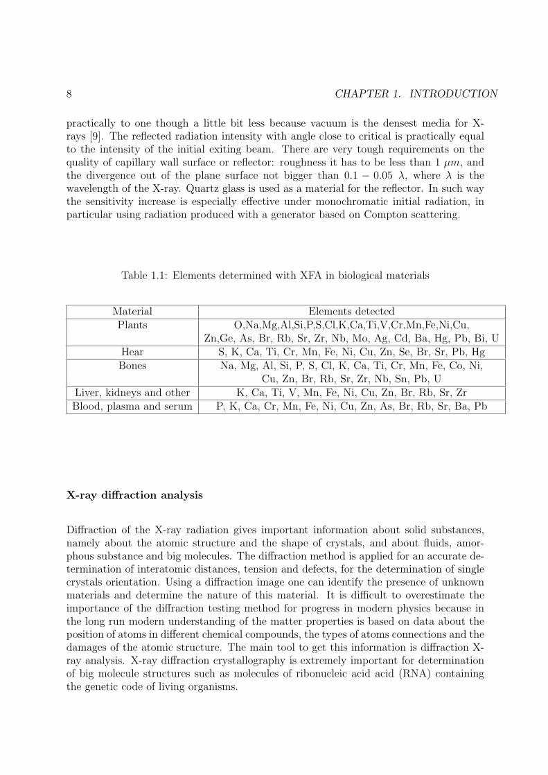
practically to one though a little bit less because vacuum is the densest media for X-rays [9]. The reflected radiation intensity with angle close to critical is practically equalto the intensity of the initial exiting beam. There are very tough requirements on thequality of capillary wall surface or reflector: roughness it has to be less than 1 µm, andthe divergence out of the plane surface not bigger than 0.1 − 0.05 λ, where λ is thewavelength of the X-ray. Quartz glass is used as a material for the reflector. In such waythe sensitivity increase is especially effective under monochromatic initial radiation, inparticular using radiation produced with a generator based on Compton scattering.
Table 1.1: Elements determined with XFA in biological materials
Material Elements detectedPlants O,Na,Mg,Al,Si,P,S,Cl,K,Ca,Ti,V,Cr,Mn,Fe,Ni,Cu,
Zn,Ge, As, Br, Rb, Sr, Zr, Nb, Mo, Ag, Cd, Ba, Hg, Pb, Bi, UHear S, K, Ca, Ti, Cr, Mn, Fe, Ni, Cu, Zn, Se, Br, Sr, Pb, HgBones Na, Mg, Al, Si, P, S, Cl, K, Ca, Ti, Cr, Mn, Fe, Co, Ni,
Cu, Zn, Br, Rb, Sr, Zr, Nb, Sn, Pb, ULiver, kidneys and other K, Ca, Ti, V, Mn, Fe, Ni, Cu, Zn, Br, Rb, Sr, ZrBlood, plasma and serum P, K, Ca, Cr, Mn, Fe, Ni, Cu, Zn, As, Br, Rb, Sr, Ba, Pb
X-ray diffraction analysis
Diffraction of the X-ray radiation gives important information about solid substances,namely about the atomic structure and the shape of crystals, and about fluids, amor-phous substance and big molecules. The diffraction method is applied for an accurate de-termination of interatomic distances, tension and defects, for the determination of singlecrystals orientation. Using a diffraction image one can identify the presence of unknownmaterials and determine the nature of this material. It is difficult to overestimate theimportance of the diffraction testing method for progress in modern physics because inthe long run modern understanding of the matter properties is based on data about theposition of atoms in different chemical compounds, the types of atoms connections and thedamages of the atomic structure. The main tool to get this information is diffraction X-ray analysis. X-ray diffraction crystallography is extremely important for determinationof big molecule structures such as molecules of ribonucleic acid acid (RNA) containingthe genetic code of living organisms.

1.1. APPLICATIONS OF HIGHT ENERGY X-RAYS 9
Methods of diffraction analysis
Laue Method
In the Laue method a continuous (”white”) spectrum of X-rays is directed on a fixedcrystal. For specific values of period d the whole spectrum wavelength satisfying Bragg lawis chosen automatically. So, the Lauegramms obtained in such way can be used to estimatethe directions of diffracted rays and, hence, the orientation of crystals planes, crystalssymmetry and to conclude important deduction about the presence of imperfections inthe crystal, the white dots corespond to diffracted X-rays. In figure 1.1 an example ofLauegramm [9] is presented. X-ray film was installed on the opposite side of the initialX-ray beam.
Figure 1.1: Lauegramm. X-rays with wide spectrum distribution pass through a fixedcrystal. X-ray diffracted beams on the Lauergramm correspond to the spots. [9]
Debye-Scherrer method.
In the Debye-Scherrer method monochromatic X-ray radiation is used at fixed wave-length (λ), but the angle of incidence θ is varied. This allows to use objects made ofmany small crystals with random space orientation such as powder. Diffracted beamsform cones with axes along the initial X-ray beam. The angle between the beam axisand the ring is called the scattering angle (θ). According to Bragg’s law, each ring corre-

10 CHAPTER 1. INTRODUCTION
sponds to a particular reciprocal lattice vector G in the sample crystal. This leads to thedefinition of the scattering vector as: G = 4π
λsin(1/2θ).
Debyegramm obtained in such way is shown in figure 1.2 contains accurate informationabout space period d, i.e. about structure of the crystal [9] As the informations obtainedfrom Debyegramm and Lauegramm are different, the two method complement each other.
Figure 1.2: Debyegram produced by passing an X-ray beam trough multi-crystals object.Each line is caused by diffraction of initial X-ray radiation on one separate plane of atoms[9].
Two beams differential angiography
Diseases of the human cardiovascular system are the most wide spread among the pop-ulation of industrial countries. This leads to high rate of disablement and as a result toa top position among reasons of human death. Early diagnostic of these diseases is veryimportant for choice of medical treatment strategy and forecast of patient life. In diag-nostics the preferences are taken to the safest and the most accurate methods of testing.Obtaining high-quality images of human organs and blood vessels is extremely importantin diagnostic and treatment of different diseases. During the last decades many phys-ical methods of visualization such as X-rays, ultrasonic, radioisotopes, impedance andothers were developed. Development of the visualization methods required joint effortsof physicists, chemists, engineers and physicians. Some other methods are less harmfulfor humans than X- rays (NMR, ultrasonic), but at the moment no single method cansubstitute to X-ray diagnostic completely [10].
Radiological investigations of arteries and veins after injection of contrast substance(angiography) is used for the diagnostic of heart disease and imperfections of cardio-vascular system of human being. Angiography allows to find inflammatory, tumor andparasitical affections of human organs and assists to choose the most rational method ofdisease treatment. Angiography studies the functional state of vessels and blood current.The methods of image production with the help of X-rays have been under developmentsince the X-ray discovery in 1895 by Wilhelm Roentgen.
The physical processes of radiation interaction with substance are the foundation ofany method of medical image visualization. It has to be noted that the object investigatedhas to be semitransparent to radiation. Therefore, in case of full absorption of radiationand total absence of interaction it is impossible to get any image of an object. X-rayphoton interacting with the electron shell of atoms of the substance investigated can ejectelectrons from the shell (photoelectric effect) or be scattered on the electrons of the targetatoms by Compton effect. For quantitative description the statistical characteristics of
1.1. APPLICATIONS OF HIGHT ENERGY X-RAYS 11
these processes the value of cross section of the interaction is used. The cross sectionsof the statistical processes determines the probability of absorption or transmission of aphoton through the substance. The values of the cross sections depends on the electrondensity of the substance, i.e. on atomic number Z and on the photon energy. With higherX-ray (photon) energy the cross sections of both processes are decreased exponentially asshown in figure 1.3 [11].
The Compton scattering cross section decreases smoothly as a function of energycharacter of decreasing while the line of the photoelectric effect cross section has sharpjumps due to threshold character of electron ejected out of the atomic shell. A photonwith energy Eγ less than binding energy in an atom Eb can not eject the electron out ofits orbit.
For an X-ray photon with an energy Eγ > Eb the value of the probability to eject anelectron is increased by step function. In general X-ray diagnostic systems the dependenceof interaction cross section on the atomic number of the object investigated Z is used. Thebase for two beams X-ray angiography is the dependence of the interaction cross sectionon the X-ray photon energy. In the photon energy range we are interested in (1−100keV )the photoelectric effect is the dominating process of the X-ray radiation interaction witha substance. Under photoelectric effect an initial photon is absorbed transferring itsenergy to an electron of an atom and eject it out of the atomic shell. The energy of theemitted electron is equal to energy of the absorbed photon minus the binding energy ofthe electron in the shell of the atom. The absorption function of the radiation due to thecross section of the process has a decreasing exponential character with sharp jumps atphoton energy values which correspond to binding energies of the electron shells. Todayiodine compounds are the most widespread X-ray contrast substance used in medicaldiagnostic systems. For iodine the rate of the jump in cross section of photon absorptionat K-edge of absorption is equal to 8. This means that in an iodine substance a photonwith energy, for example, 33.1 keV will be absorbed with a probability 8 times less thana photon with energy 33.2 keV . The tissue and bones of a human body are equallytranslucent for X-ray photons of these energies, i.e. the probability of photon absorptionis the same for both items. If one can get the first image for flux of photons with energy33.1 keV (monochromatic X-ray beam) and the second image for flux of photons withenergy 33.2 keV the image of the radiation absorption with bones and other tissues willbe the same for both cases while absorption with X-ray contrast substance will be quitedifferent. So, fixing the images in digital data and then subtracting one from anotherone can separate the image of vessels with contrast substance. Hence, for two beamsX-ray angiography method realization one has to have two monochromatic, collimatedX-ray beams, scanning systems, two registration systems for transmitted X-ray beamsregistration with high positioning accuracy and software of processing and visualizationof the images produced.
The development of a project of coronary angiography of humans has been initiated inStanford Linear Accelerator Center (SLAC) as early as 1979 [12], [13]. Today angiographyusing synchrotron radiation has become the general method of investigation and diagnostic

12 CHAPTER 1. INTRODUCTION
Figure 1.3: Absorption coefficients of iodine, bone and soft tissue. [11]
of ischemia in industrialised countries. The further development of the method makes ituseful not only for the diagnostic of coronary vessels in initial stage of myocardium infarctbut also for general estimation of the state of cardiovascular system of an individual. Inthe USA more then one million angiogrames are produced every year and this number isgrowing. The method is becoming more common in Europe and Japan too.
In figure 1.4 the layout of angiogram production at a synchrotron radiation source ispresented [14].
For the procedure described above the following photon beam parameters are required:
1. Photon beam energy above E0 = 33.156 keV for iodine and below E0 = 50.329 keVfor gadolinium
2. Photon beam intensity: 9.10 ∗ 1010 phot/mm2s
3. Energy spread of photon beam: ±150 eV
4. Monochromatic photon beam size: better than 0.1× 150 mm2.
5. Time of exposure: less than 2 µs.

1.1. APPLICATIONS OF HIGHT ENERGY X-RAYS 13
Figure 1.4: The typical experimental set-up for transvenous coronary angiography withsynchrotron radiation. [14]
With these requirements the method allows to get an image of the cardiovascularsystem with a resolution of about 0.5× 0.5 mm2.
From the requirements of angiographic devices presented above it follows that forsuccessful realization of the method on the base of Compton scattering X-ray generatorthe following tasks have to be done:
1. Production of photon beam with energy E0 = 33.156 ± 0.15 keV with intensity ofabout 1011 − 1012 phot/(mm2 × s).
2. Development of a monochromator and optical system to transport photon beam(beam line) satisfying the above requirements.
3. Development of the whole beam line for coronary angiography including problemswith installation and alignment of optical elements of the beam line.
4. Development of a detection system for the photon beam.
5. Development of a control system of the beam line.
6. Development of software.
Two beams X-ray angiography is a highly efficient, safe, profitable method of beamdiagnostics. The conditions of angiography realization are development and constructionof modern sources of X-ray radiation (synchrotron radiation sources, X-ray generatorsbased on Compton Scattering); development of flat digital detector of X-rays allows toproduce X-ray images in digital form with high speed of data collection and very lowradiation dose.

14 CHAPTER 1. INTRODUCTION
1.2 Compton back scattering
Compton back scattering is the collision of a photon with a relativistic electron. We definethe photon’s energy as ε0, the electron energy as E0, the rest energy of the electron asmc2 and γ = E0/mc2 and we assume E0 ≫ ε0. The photons will be scattered in a conewith an opening angle of ∼ 1/γ around the direction of motion of the electrons. Thekinematic of the scattering process is presented in figure 1.5. We will consider the case oflinear Compton back scattering. We neglect the probability of simultaneous collision ofone electron with two and more photons.
Figure 1.5: Kinematics of the scattering process.
We will use the model presented in [15] . Energy of scattered photon εγ is dependenton the angle θγ as:
εγ =εγm
1 +(
θγθ0
)2 (1.1)
where εγm is the maximum scattered photon energy, θ0 =mc2
E0
√x+ 1, with
x =4Eεγ0(mc2)2
cos2α0
2(1.2)
εγ0 is the energy of the laser photon. Photons with energy εγ > εγm are scatteredangle θγ > θ0, and photons with energy εγ < εγm are scattered photons θγ < θ0.
1.2. COMPTON BACK SCATTERING 15
Now rewrite θγ from (1.1):
θγ = θ0
√
εγmεγ
− 1 (1.3)
Introducing a new parameter normalized phonon energy on electron energy
y =εγE0
≤ ym =εγmE0
=x
(x+ 1)(1.4)
we can write the scattered photon angle as function of it’s energy in the following form:
θγ(y) = θ0
√
ymy
− 1 (1.5)
Then scattering electron angle is:
θe(y) = θγy
1− y(1.6)
Now expand expression for maximum energy of scattered photons and replacing γ = E0
mc2
εγm =4γ2εγ0 cos
2 α0
2
4γ εγ0mc2
cos2 α0
2+ 1
(1.7)
Then in case of a small interaction angle between the photon and the electron beamsα0 ≪ 1 and with the condition 4γ2 ≪ E0
εγ0, it means that the energy of the scattered
photon is much less than the energy of the electron beam and we will have:
εγm ≈ 4γ2εγ0 (1.8)
It means that using relativistic electron bunches with relatively small energy we canreceive radiations with energy in X-ray range. For example for an electron beam energy50 MeV the maximum photon energy will be 45 keV .
Substituting (1.8) in (1.5) and (1.7). Then we get:

16 CHAPTER 1. INTRODUCTION
θ0 =1
γ
√
4γεγ0mc2
− 1 ≈ 1
γ(1.9)
and substituting (1.9) in (1.1) we can write the scattered photon energy dependenceon the scattering angle:
εγ =4γ2εγ01 + θ2γγ
2=
4εγ01γ2 + θ2γ
(1.10)
The maximum scattered photon energy εγm versus the electron beam energy E0 fora laser with photon energy εγ0 = 1.24 eV or λ = hc
εγ0= 1 µm is shown in figure 1.6.
It is clear that it is possible to produce a photon beam with photon in an energy rangefrom keV up to several MeV . This covers up most of all needs of all known science andtechnological applications of the X-rays and γ-rays.
0 50 100 150 200 2500
0.2
0.4
0.6
0.8
1
1.2
1.4
E0 [MeV ]
εγ0 = 1.24 [eV ]; α0 ≪ 1;
εγm[M
eV]
Figure 1.6: Dependence of the maximum scattered photon energy on the energy of theelectrons for a laser photons energy εγ0 = 1.24 eV .
1.2.1 Compton cross-section
The energy spectrum of scattered photons is differential cross-section of a linear Comptonscattering in laboratory coordinate system been given by [16]:
1.2. COMPTON BACK SCATTERING 17
1
σc
dσc
dy≡ f(x, y) =
2σ0
xσc
[
1− y +1
1− y− 4r(1− r) + 2λePcrx(1− 2r)(2− y)
]
(1.11)
where λe - is the average helicity of an electron, Pc - is the degree of circular polarization(equal to an average helicity) | λe |≤ 1
2; | Pc |≤ 1
2and total Compton cross-section σc
is defined as the sum of the non polarized cross-section σnpc with the polarisation term
2λePσ1:
σc = σnpc + 2λePσ1 (1.12)
σnpc =
2σ0
x
[(
1− 4
x− 8
x2
)
ln(x+ 1) +1
2+
8
x− 1
2(x+ 1)2
]
(1.13)
σ1 =2σ0
x
[(
1 +2
x
)
ln(x+ 1)− 5
2+
1
x+ 1− 1
2(x+ 1)2
]
(1.14)
r =y
x(1− y)(1.15)
σ0 = π
(
e2
mc2
)
= 2.5 ∗ 10−29 m2 (1.16)
As shown on equetion 1.11 and [17] the influence of polarization effects on the differen-tial cross-section of Compton scattering becomes noticeable when the initial electron beamenergy E0 is about 5 GeV . The differential cross-section of a linear Compton scatteringfor different energy of electrons beam is presented in figure 1.7.
Also it should be noted the significant dependence of the differential cross-section ofa linear Compton scattering on initial energy of electron beam. This fact has to be takeninto account in numerical calculations with electron beam with energy spread of about oneor more percent. The formula 1.5 gives the dependence of the angle of scattered photonson their energy, their angular distributions in unit of solid angle dΩ can be written as:
dσ
dΩ=
σc
πθ20
ymf(x, y(θγ))(
1 +(
θγθ0
)2)2 (1.17)
where y(θγ) =ym
1+(θγ/θ0).
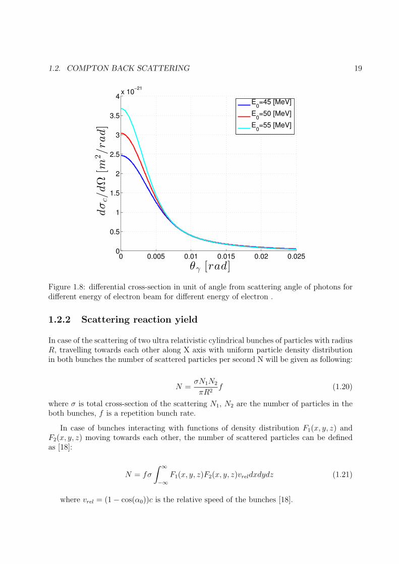
The dependence of the differential cross-section in unit of solid angle from the scat-tering angle of photons for different energy of electron beam is presented in figure 1.8.
The angular spectrum of the scattered photons in the plane of interaction:

18 CHAPTER 1. INTRODUCTION
0 10 20 30 40 505
6
7
8
9
10
11
12
13x 10
−22
εγ [keV ]
dσc/dy[m
2]
E0=45 [MeV]
E0=50 [MeV]
E0=55 [MeV]
Figure 1.7: Energy spectrum of scattered photons for different energy of electron beamE0: red E0 = 45MeV , blue E0 = 50MeV , green E0 = 55MeV .
dσ
dΩ=
dσ
2πθγdθγ(1.18)
accordingly:
dσ
dθγ= 2πθγ
dσ
dΩ(1.19)
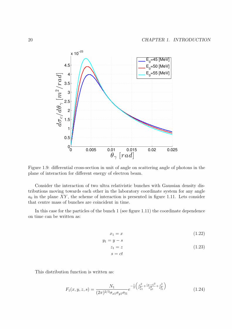
Differential cross-section in unit of angle on scattering angle of photons in the planeof interaction is presented in figure 1.9.
According to equation (1.5) by replacing θγ by θ0√
εγmεγ
− 1 in to (1.17) we get the
energy spectrum of the scattered photons in unit of solid angle. The differential cross-section in unit of solid angle in dependence of energy of scattered photons is presented onfigure 1.10
1.2. COMPTON BACK SCATTERING 19
0 0.005 0.01 0.015 0.02 0.0250
0.5
1
1.5
2
2.5
3
3.5
4x 10
−21
θγ [rad]
dσc/dΩ
[m2/rad]
E0=45 [MeV]
E0=50 [MeV]
E0=55 [MeV]
Figure 1.8: differential cross-section in unit of angle from scattering angle of photons fordifferent energy of electron beam for different energy of electron .
1.2.2 Scattering reaction yield
In case of the scattering of two ultra relativistic cylindrical bunches of particles with radiusR, travelling towards each other along X axis with uniform particle density distributionin both bunches the number of scattered particles per second N will be given as following:
N =σN1N2
πR2f (1.20)
where σ is total cross-section of the scattering N1, N2 are the number of particles in theboth bunches, f is a repetition bunch rate.
In case of bunches interacting with functions of density distribution F1(x, y, z) andF2(x, y, z) moving towards each other, the number of scattered particles can be definedas [18]:
N = fσ
∫ ∞
−∞F1(x, y, z)F2(x, y, z)vreldxdydz (1.21)
where vrel = (1− cos(α0))c is the relative speed of the bunches [18].
20 CHAPTER 1. INTRODUCTION
0 0.005 0.01 0.015 0.02 0.0250
0.5
1
1.5
2
2.5
3
3.5
4
4.5
x 10−23
θγ [rad]
dσc/dθγ[m
2/rad]
E0=45 [MeV]
E0=50 [MeV]
E0=55 [MeV]
Figure 1.9: differential cross-section in unit of angle on scattering angle of photons in theplane of interaction for different energy of electron beam.
Consider the interaction of two ultra relativistic bunches with Gaussian density dis-tributions moving towards each other in the laboratory coordinate system for any anglea0 in the plane XY , the scheme of interaction is presented in figure 1.11. Lets considerthat centre mass of bunches are coincident in time.
In this case for the particles of the bunch 1 (see figure 1.11) the coordinate dependenceon time can be written as:
x1 = x (1.22)
y1 = y − s
z1 = z (1.23)
s = ct
This distribution function is written as:
F1(x, y, z, s) =N1
(2π)2/3σx1σy1σl1
e− 1
2
(
x2
σ2x1
+(y−s)2
σ2y1
+ z2
σ2l1
)
(1.24)

1.2. COMPTON BACK SCATTERING 21
0 10 20 30 40 500
0.5
1
1.5
2
2.5
3
3.5
4x 10
−21
εγ [keV ]
dσc/εγ[m
2/eV]
E0=45 [MeV]
E0=50 [MeV]
E0=55 [MeV]
Figure 1.10: differential cross-section in unit of solid angle in dependence of energy ofscattered photons for different energy of electron beam.
where σx1, σy1 is transverse size, σl1 is longitudinal size of bunch 1.
For particles of the bunch 2 (see figure 1.11) the time dependence of the coordinateswill be:
x1 = − cos(α0)x− sin(α0)y (1.25)
y1 = sin(α0)x− cos(α0)y − s
z1 = z,
And the distribution function is written as:
F2(x, y, z, s) =N2
(2π)2/3σx2σy2σl2
e− 1
2
(
x2
σ2x2
+(y−s)2
σ2y2
+ z2
σ2l2
)
(1.26)
where σx2, σy2 is transverse size, σl2 is longitudinal size of bunch 2.
After integration of equation (1.21) we the get number of scattered particles in unitof time.

22 CHAPTER 1. INTRODUCTION
Figure 1.11: Interaction between two bunches with Gaussian density distributions.
N =1
√2π√
σ2y1 + σ2
y2
σN1N2f√
σ2x1 + σ2
x2 + (σ2z1 + σ2
z2) tan(α0
2)
(1.27)
In case the bunches do not cross the interaction point at the same time, let’s call ∆x,∆y then transverse misalignment and ∆z the longitudinal misalignment. The number ofscattered photons becomes [19]:
N =AyAxAz
√2π√
σ2y1 + σ2
y2
σN1N2f√
σ2x01 + σ2
x2 + (σ2z1 + σ2
z2) tan(α0
2)
(1.28)
where
Ay = exp
(
− ∆y2 tan2(α0)
2(σ2x1 + σ2
x2 + (σ2z1 + σ2
z2) tan(α0
2))
)
Ax = exp
(
− ∆x2
2(σ2x1 + σ2
x2 + (σ2z1 + σ2
z2) tan(α0
2))
)
Az = exp
(
− ∆z2
2(σ2y1 + σ2
y2)
)

1.2. COMPTON BACK SCATTERING 23
1.2.3 Numerical simulation
For the numerical simulations of Compton scattering we use the code CAIN writtenby K. Yokoya. CAIN is a stand-alone FORTRAN Monte-Carlo code for the interactioninvolving high energy electrons, positrons, and photons [20]. The main advantage of usingthis code for us it is that the code CAIN give to us possibility of using non Gaussiandistribution of electrons. This give us the possibility to integrate the code CAIN as afunction in a 6D tracking code to simulate Compton scattering with longitudinal andtransverse dynamics of the electron bunch, to see the evolution of the electron beamunder Compton scattering in the ring and how this evolution will influence the flux ofscattered photons.
This code was already bench-marked [21, 22]. A comparison of the analytical calcula-tion of the flux of scattered photons with a longitudinal laser misalignment and result ofnumerical simulations made in CAIN is shown in figure 1.12.
For this comparison was done set of the simulations in CAIN for different longitudinallaser misalignment and compare with analytical calculation made by using equation 1.28.
Figure 1.12: Comparison of the theoretical formula 1.29 for the Compton flux (in red) withthe flux calculated by simulations in CAIN (in blue). The horizontal axis corresponds todifferent misalignments of the longitudinal laser position (laser timing) at the interactionpoint.
As we we can see in figure 1.12 numerical simulations made by the code CAIN haveexcellent agreement with the analytical approach.

24 CHAPTER 1. INTRODUCTION
1.3 General Layout and working scheme of the ThomX
X-ray generator
ThomX is a project of X-ray source based on the Compton scattering of laser photonsand relativistic electrons. The electron bunch is stored in a storage ring allowing tocollision it with the laser pulse on each turn. The beam life time is around 400 000 turns,corresponding to 20 ms. The use of a circular electrons storage ring give a significantadvantage over linac-based Compton sources where electrons can be used only once toproduce a high flux.
ThomX as X-ray source consists of 6 main parts which are presented in figure 1.13and listed below:
Figure 1.13: Layout of the ThomX source. [23].
1. Photo electron gun to produce electron bunch 1 nC.
2. Linear accelerating section to accelerate electrons to 50− 70 MeV .
3. Transfer line.
4. Storage ring with circumference 16.8 m.
5. Interaction Point with Fabry Perot Cavity.
6. Laser.
As we can see ThomX can be split for three main component: Injector, Ring, Laserand FP cavity.

1.3. GENERAL LAYOUTANDWORKING SCHEMEOF THE THOMXX-RAYGENERATOR25
Table 1.2: Injector
Charge 1 nCLaser wavelength and pulse power 266 nm, 100 µJ
Gun Q and Rs 14400, 49 MW/mGun accelerating gradient 100 MV/m @ 9.4 MWNormalized r.m.s emittance 8πmm mrad
Energy spread 0.36%Bunch length 3.7 ps
Table 1.3: Ring
Energy 50MeV (70MeV possible)Circumference 16.8 m
Crossing-Angle (full) 2 degreesβx,y@ IP 0.1 m
εx,y (without IBS and Compton) 3 ∗ 10−8mBunch length (@ 20 ms) 30 ps
Beam current 17.84 mARF frequency 500 MHz
Transverse / longitudinal damping time 1 s/0.5 sRF Voltage 300 kV
Revolution frequency 17.84 MHzσx@ IP (injection) 78 µm
Tune x / y 3.4 / 1.74Momentum compaction factor αc 0.022
Final Energy spread 0.6%
Table 1.4: Laser and FP cavity
Laser wavelength 1030 nmLaser and FP cavity Frep 35.68 MHz
Laser Power 50− 100 WLaser Pulse Power 1.4− 2.6 µJ
FP Cavity finesse / Gain 30000 / 10000FP waist 70 µm
Power Circulating in the FP Cavity ∼ 0.07− 0.7 MW
26 CHAPTER 1. INTRODUCTION
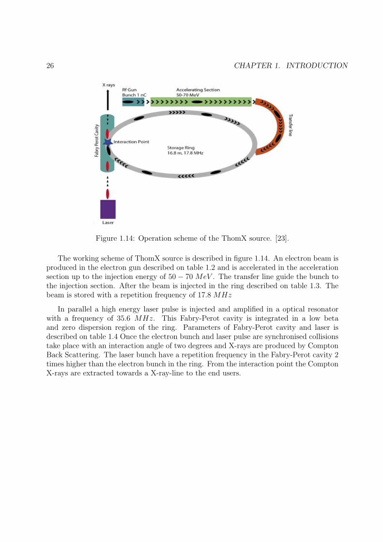
Figure 1.14: Operation scheme of the ThomX source. [23].
The working scheme of ThomX source is described in figure 1.14. An electron beam isproduced in the electron gun described on table 1.2 and is accelerated in the accelerationsection up to the injection energy of 50− 70 MeV . The transfer line guide the bunch tothe injection section. After the beam is injected in the ring described on table 1.3. Thebeam is stored with a repetition frequency of 17.8 MHz
In parallel a high energy laser pulse is injected and amplified in a optical resonatorwith a frequency of 35.6 MHz. This Fabry-Perot cavity is integrated in a low betaand zero dispersion region of the ring. Parameters of Fabry-Perot cavity and laser isdescribed on table 1.4 Once the electron bunch and laser pulse are synchronised collisionstake place with an interaction angle of two degrees and X-rays are produced by ComptonBack Scattering. The laser bunch have a repetition frequency in the Fabry-Perot cavity 2times higher than the electron bunch in the ring. From the interaction point the ComptonX-rays are extracted towards a X-ray-line to the end users.
Chapter 2
Storage ring RF system
In a low energy ring like ThomX, the natural damping time is long (∼ 1 s) that astationary stable condition can never be reached during the beam storage time, which isas short as 20 ms. On the other hand, it is sufficient to maintain the instability growthtime larger than the beam storage time in order to keep at tolerable level their effect onthe beam. That requires very strong attenuation of the cavity HOM impedances, typicallyby a few 103. There are essentially two methods of coping with such HOM impedances,either a strong de-Qing of the HOM resonances [24, 25] or a tuning of their frequenciesaway from the beam spectral lines to prevent resonant excitations. With the former it isdifficult to reach attenuation factors larger than a few 102 over a wide frequency range.The latter, which consists in controlling the HOM frequencies, is better suited to a smallcircumference machine like ThomX, where the beam spectral lines spacing (18 MHz) isvery large as compared to the HOM bandwidth. As far as the HOM density is not too highand that they can be tuned far enough from the beam spectral lines (δf ≪ fHOM/Qo),it should be possible to reduce their effective impedances (”seen” by the beam) down totolerable levels : Reff ≈ Rs/(2Qoδf/fHOM)2 ≫ Rs. That led us to choose the ELETTRAtype cavity which allows applying this technique in combining three tuning means. TheHOM frequencies are precisely controlled by proper setting of the cavity water coolingtemperature over the range 60±25C with a stability of ±0.05C, while the fundamentalfrequency is recovered by means of a mechanical tuning which changes the length of thecavity. Besides, a movable plunger provides another degree of freedom for tuning theHOM. In order to insure a fine control of the HOM frequencies, a good knowledge of theircharacteristics is mandatory. The main parameters of the fundamental and the HOMshave therefore been calculated using the Eigenmode solver of the 3D ElectromagneticHFSS [26] and CST MWS [27] codes and compared the results with the measured valueson the cavity [28].
The selection of 500 MHz as RF frequency leads to a quite good compromise in termsof cavity fundamental and HOM impedances, space requirements as well as the availabilityof RF power sources and other components.
27

28 CHAPTER 2. STORAGE RING RF SYSTEM
500 MHz RF Cavity
One 500 MHz single cell cavity of the ELETTRA type, powered with a 50 kWCW solidstate amplifier (SSA), will provide the required RF voltage of 500 kV . It is made outof OFHC copper and equipped with 8 equatorial outlet ports: 3 large ones for the inputpower coupler, the pumping system, the plunger tuner and 5 smaller ones for vacuum andRF monitoring. It is water cooled by means of copper pipes brazed on its external wallsurface. Its temperature can be set over the range 60± 25C with a stability of ±0.05Cby re-circulating the cooling water through an appropriate heat exchanger (cooling rack).The cavity cutoff tube (ø 100 mm) will be connected to the standard elliptical vacuumchamber (a=40mm, b=28mm) by means of two tapers, made of 316 L stainless steel andbellows. The cavity assembly is shown in Figure 2.1.
Figure 2.1: ThomX cavity assembly (front and back views).
500 MHz CW Solid State Amplifier (SSA)
Recently synchrotron SOLEIL has worked out modules, which can deliver up to 650 W at500 MHz with a gain of 16.5 dB and an efficiency of 64 % [29]. About a hundred of suchmodules will be combined for achieving the required 50 kW power. A 10 kW prototypeunit (16 modules) was successfully tested and validated by mid of 2012 at SOLEIL andthe complete 50 kW CW SSA will be tested on a dummy load, by the end of 2013.
Low Level RF and Feedback Systems
The task of a Low Level RF (LLRF) system is to control the amplitude and phase ofthe cavity accelerating voltage and its resonance frequency. Three LLRF prototypes,

29
including a fast longitudinal feedback (LFB) are being developed in parallel. The firstversion consists in separate analog control loops for frequency, amplitude and phase; thesecond version is based on analog IQ modulation/demodulation technique and the thirdone on digital FPGA processing. The cavity voltage shall be controlled with typicalstability of ±0.2 % and ±0.2 by means of the conventional phase and amplitude loops(either analog or digital) of few kHz bandwidths. In addition the LFB, namely a fastphase feedback, combined with a high gain RF feedback acting directly on the acceleratingcavity [30], will provide the longitudinal damping of a few 10 µs, which is required topreserve the beam quality during its storage time of 20ms. This LFB shall cope withthe beam oscillations, caused by injection transients as well as by the longitudinal HOMexcitations, in addition to the frequency tuning technique. Besides, a transverse feedback(TFB), based on FPGA processing, similar to that used in SOLEIL [31], and acting on adedicated stripline kicker shall cope with the transverse modes of both planes, horizontal(H) and vertical (V).
Simulations and measurements
The characteristic parameters of a cavity mode are its resonant frequency, its unloadedquality factor Q0, its R/Q (shape factor) and its shunt impedance, Rs = (R/Q).Q0. Theyhave been computed with the HFSS and CST MWS codes using Eigenmode solver withcylindrical symmetry for the longitudinal and transverse modes of the cavity, includingits 30 cm long stainless steel tapers. On the other hand, the frequency and the loadedquality factor, QL of the modes have been measured on the cavity at ambient temper-ature and under vacuum using a vector network analyzer (VNA) in transmission mode.The unloaded quality factor Q0 values are deduced by taking into account the couplingcoefficients of the input power coupler and monitoring pick-up.
Fundamental Mode Parameters
Table 2.1 shows a comparison between the computer simulations and measurements I didof the parameters of the accelerating mode, that is the TM010 fundamental mode of thecavity. The shunt impedance is defined as Rs = V 2
acc/2Pd, where Vacc is the acceleratingvoltage (transit time factor included) and Pd is the cavity wall dissipation.
HOM Parameters
Simulations and measurements have been performed also for the HOMs of the cavity,terminated with its two tapers. The results are listed, in Table 2.2 and 2.3 for themonopole and dipole modes, which are trapped into the cavity, namely with a resonancethat is lower than its tube (ø 100 mm) cut-off frequencies, 2.3 GHz for monopole and1.83 GHz for dipole modes. The two polarizations, H and V, of the dipole modes, are not
30 CHAPTER 2. STORAGE RING RF SYSTEM
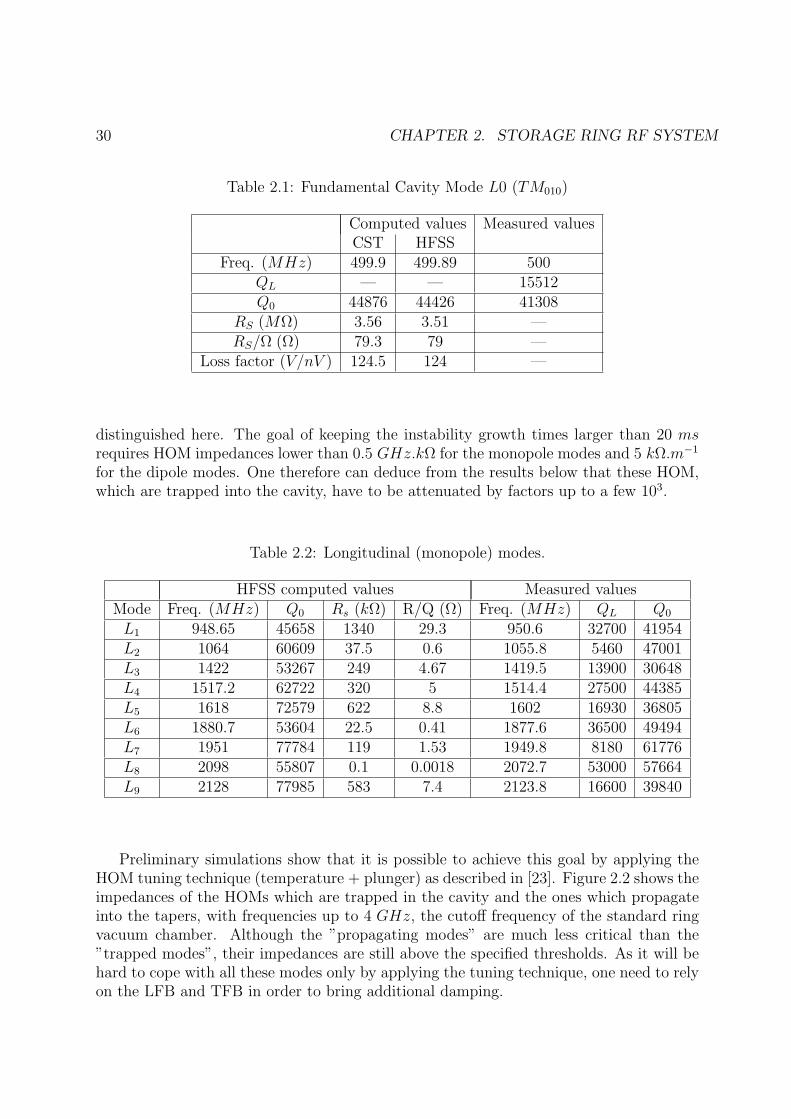
Table 2.1: Fundamental Cavity Mode L0 (TM010)
Computed values Measured valuesCST HFSS
Freq. (MHz) 499.9 499.89 500QL — — 15512Q0 44876 44426 41308
RS (MΩ) 3.56 3.51 —RS/Ω (Ω) 79.3 79 —
Loss factor (V/nV ) 124.5 124 —
distinguished here. The goal of keeping the instability growth times larger than 20 msrequires HOM impedances lower than 0.5 GHz.kΩ for the monopole modes and 5 kΩ.m−1
for the dipole modes. One therefore can deduce from the results below that these HOM,which are trapped into the cavity, have to be attenuated by factors up to a few 103.
Table 2.2: Longitudinal (monopole) modes.
HFSS computed values Measured valuesMode Freq. (MHz) Q0 Rs (kΩ) R/Q (Ω) Freq. (MHz) QL Q0
L1 948.65 45658 1340 29.3 950.6 32700 41954L2 1064 60609 37.5 0.6 1055.8 5460 47001L3 1422 53267 249 4.67 1419.5 13900 30648L4 1517.2 62722 320 5 1514.4 27500 44385L5 1618 72579 622 8.8 1602 16930 36805L6 1880.7 53604 22.5 0.41 1877.6 36500 49494L7 1951 77784 119 1.53 1949.8 8180 61776L8 2098 55807 0.1 0.0018 2072.7 53000 57664L9 2128 77985 583 7.4 2123.8 16600 39840
Preliminary simulations show that it is possible to achieve this goal by applying theHOM tuning technique (temperature + plunger) as described in [23]. Figure 2.2 shows theimpedances of the HOMs which are trapped in the cavity and the ones which propagateinto the tapers, with frequencies up to 4 GHz, the cutoff frequency of the standard ringvacuum chamber. Although the ”propagating modes” are much less critical than the”trapped modes”, their impedances are still above the specified thresholds. As it will behard to cope with all these modes only by applying the tuning technique, one need to relyon the LFB and TFB in order to bring additional damping.

31
Figure 2.2: Shunt impedance spectrum for (a) monopole and (b) dipole modes.

32 CHAPTER 2. STORAGE RING RF SYSTEM
Table 2.3: Transverse (dipole) modes.
CST computed values Measured valuesMode Freq. (MHz) Q0 Rs (kΩ) R/Q (Ω) Freq. (MHz) QL Q0
D1 744.2 47966 3.6 76 742.4 44300 47046D2 749.4 50421 13 258 745.5 7640 42631D3 1114 40971 12.8 314 1115 17880 52316D4 1224 95336 0.23 2.55 1213.4 57000 58220D5 1250 39726 4.5 114 1239.7 35400 37240D6 1311 62710 0.2 3.1 1303 49900 52595D7 1561 29480 0.03 1 1556 18200 26172D8 1643 40494 3.2 79 1646 30900 33372D9 1717 75798 1.3 17.5 1711.4 26500 27825D10 1723 44231 2.3 50.5 1718.3 58500 58815D11 1779 46762 1.6 33 1770.3 39200 45315D12 1811 38748 1.24 32 1820 31900 37515
Adjustable HOM Frequency Shifter (HOMFS)
The HOMFS is a plunger moving into one of the three equatorial ports, as shown inFigure 2.1, for shifting the resonant frequencies of harmful HOMs if a stable conditioncannot be achieved only by temperature tuning. Figure 2.3 shows the HOMFS effectson the trapped monopole and dipole modes for its full displacement range of 35 mm.The fundamental as well as the HOM frequencies vary linearly with the plunger position.Except for a few modes which are less sensitive, frequency shifts of 1 MHz or more areachieved.
Electromagnetic parameter calculations using CST and HFSS codes as well as mea-surements have been performed on the ThomX cavity. The results show that a strongattenuation of the cavity HOM impedances is required in order to preserve the beam qual-ity in the storage ring. It will be achieved by a proper control of the HOM frequenciesin combining three tuning means and by the use of feedbacks for providing additionaldamping.
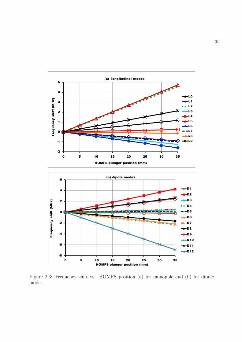
33
Figure 2.3: Frequency shift vs. HOMFS position (a) for monopole and (b) for dipolemodes.

34 CHAPTER 2. STORAGE RING RF SYSTEM

Chapter 3
Beam dynamics at ThomX
In this chapter I describe the theoretical models of beam dynamics which I use in thesimulation code. The 6D beam dynamics can be split in two main part the transversemotion and the longitudinal motion. They are coupled by non diagonal elements in thetransport matrices or by the coupled system of the equations of motion in Hamiltonianformalism. In this chapter I also present models of calculation for collective effects suchas longitudinal space charge, resistive wall, coherent synchrotron radiation and intrabeamscattering.
3.1 Models of transverse motion at circular acceler-
ators
There are two main models to describe transverse motions of charged particles in a circularaccelerators:
• Transport matrices.
• The Hamiltonian Formalism with Perturbation theory.
3.1.1 Transport matrices model
The motion of a particle in a magnetic field can be described in local coordinate systemmoving jointly with the particle by the arbitrary curve determined by the curvatureh = 1
ρ= dφ
dsby the moving equations:
35
36 CHAPTER 3. BEAM DYNAMICS AT THOMX
x′′ − h2x = −h− hxx′ + 2hx′2
1− hx+ (3.1)
e
pc
√
1 +
(
x′
1− hx
)2
(x′y′Bx − [(1− hx)2 + x′2]By + (1− hx)z′Bs)
y′′ = −hxy′ + 2hx′y′
1− hx+ (3.2)
e
pc
√
1 +
(
x′
1− hx
)2
(x′y′Bx − [(1− hx)2 + x′2]By + (1− hx)z′Bs)
Where Bx, By, Bs are the component of the magnetic field, p is the momentum ofthe particle, ρ is the radius of curvature for the synchronous particle, φ is the azimuthalangle of the bending magnet.
The solution of equations 3.1, 3.2 may be represented in a matrix form. This matrixis introduced in works of A. Chao [32].
Using matrices we can change a coordinates of particle in phasespace due to propaga-tion through the magnetic elements into the accelerator.
x2
x′2
y2y′2s2δe 2
= Mfrom 1to 2
x1
x′1
y1y′1s1δe 1
(3.3)
Knowing all matrices for each element of the accelerator we can obtain the totaltransport matrix of the accelerator
MTOT = Mn ∗Mn−1 ∗ ... ∗M2 ∗M1 (3.4)
Using only one transport matrix for all accelerator makes the simulations faster incomparison with propagation element by element.
We can also make the propagation element by element:

3.1. MODELS OF TRANSVERSE MOTION AT CIRCULAR ACCELERATORS 37
xn
x′n
yny′nsnδe n
= Mfrom n−1 to n
xn−1
x′n−1
yny′n−1
snδe n−1
...
x2
x′2
y2y′2s2δe 2
Mfrom 1to 2
x1
x′1
y1y′1s1δe 1
(3.5)
Thanks to this matrix we can estimate all the main parameters of the beam and checkif the coordinates of the particles do not go out of the acceptance of the accelerator.
The matrix of the main electromagnetic elements of accelerator structures were cal-culated by K. L. BROWN [33].
Drift element:
1 L 0 0 0 00 1 0 0 0 00 0 1 L 0 00 0 0 1 0 00 0 0 0 1 00 0 0 0 0 1
(3.6)
Where L is the length of the drift space.
Quadrupole lens:
cos√KL sin
√KL√K
0 0 0 0
−√K sin
√KL cos
√KL 0 0 0 0
0 0 cosh√KL sinh
√KL√
K0 0
0 0√K sinhKL cosh
√KL 0 0
0 0 0 0 1 00 0 0 0 0 1
(3.7)
Where L is the effective length of the quadrupole lens, K = eGpc
is the force of the
quadrupole lens, G = ∂By
∂y= ∂Bx
∂xis the gradient of magnetic field.
Bending magnet (dipole):
cosAxsinAx√
Kx0 0 0 h√
Kx(1− cosAx)
−√Kx sinAx cosAx 0 0 0 − h√
KxsinAx
0 0 coshAysinhAy√
Ky0 0
0 0 −√
Ky sinhAy coshAy 0 0− h√
KxsinAx − h√
Kx(1− cosAx) 0 0 1 − h
K3/2x
(Ax − sinAx)
0 0 0 0 0 1
(3.8)

38 CHAPTER 3. BEAM DYNAMICS AT THOMX
with Ax =√KxL, Ay =
√
KyL, where L is the effective length of the orbit of the
synchronous particle inside a bending magnet, Kx = (1 − n)h2, Ky = nh2, n = − ρB0
∂B∂x
is the normalized field gradient of the bending magnet measured on optical axes (x =0, y = 0). In case of uniform field (n = 0, Kx = h2 = (1/ρ)2, Ky = 0 ) the matrix for thebending magnet becomes simple.
cos√KxL
sin√KxL√Kx
0 0 0 h√Kx
(1− cos√KxL)
−√Kx sin
√KxL cos
√KxL 0 0 0 − h√
Kxsin
√KxL
0 0 1sinh
√KyL√
Ky0 0
0 0 0 1 0 0− h√
Kxsin
√KxL − h√
Kx(1− cos
√KxL) 0 0 1 − h
K3/2x
(√KxL− sin
√KxL)
0 0 0 0 0 1
(3.9)
Transport matrices can be used to obtain linear characteristics of the magnetic struc-ture of the accelerator and their characteristic. Matrices allow to make linear particletracking, but due to limited accuracy for a large number of turns the rounding errors inthe matrices will accumulate. It is also difficult to take in to account non linear effectsusing method of transport matrices.
3.1.2 The Hamiltonian Formalism
The Hamiltonian Formalism has several uncontested advantages:
• Opens the possibility to consider nonlinear forces in the same way as linear;
• The method allows to obtain not only the solutions of equations of motion, but alsothe integrals of motion.
In this chapter we go briefly through the basic concept of Hamiltonian formalism toobtain the dynamics in accelerators. In real space we can write the Lagrangian L(q, q, t),where q is the coordinate and q is the time derivative of it, t is the time, i = x, y, s:
L(qi, qi, t) = T (qi)− U(qi, t) (3.10)
here T is the kinetic energy and U is the potential energy. Then the equation ofmotion in Lagrange form:
d
dt
∂L
∂qi− ∂L
∂qi= Qi (3.11)
3.1. MODELS OF TRANSVERSE MOTION AT CIRCULAR ACCELERATORS 39
here Qi is forces not defined from a potential.
The Hamiltonian can be defined as:
H(p, q, t) =∑
i
qipi − L(qi, qi, t) (3.12)
and in this case the equations of motion can be rewritten with the first derivative only:
p = −(
∂H
∂qi
)
+Qi; qi =∂H
∂qi;∂L
∂t= −∂H
∂t; (3.13)
where p is the canonical momentum. If Qi = 0 all forces can be described by potentials(see equation 3.13) and can be reduced to canonical Hamiltonian equations:
p = −(
∂H
∂qi
)
; qi =∂H
∂qi; (3.14)
where H(pi, qi, t) represent the energy of the system, pi, qi the momentum and coor-dinate of the particles.
Solving equations 3.14 for p, q as functions of time give us the possibility to follow thetrajectory of the particle in phasespace (p, q).
Canonical transformation is changing of canonical coordinates (q, p, t) → (Q,P, t)can be done by using the generating function [34].
G1(qi, Qi) : pi =∂G1
∂qi; Pi =
∂G1
∂Qi
; H = H +∂G1
∂t; (3.15)
G2(qi, Pi) : Qi =∂G2
∂Pi
; pi =∂G2
∂Qi
; H = H +∂G2
∂t; (3.16)
G3(pi, Pi) : qi = −∂G3
∂qi; Qi =
∂G3
∂Qi
; H = H +∂G3
∂t; (3.17)
G4(Qi, Pi) : qi = −∂G4
∂qi; Pi = −∂G4
∂Qi
; H = H +∂G4
∂t; (3.18)
Using the canonical transformations 3.15-3.18 it is possible to transform the initialequations 3.14 to a form easier to solve.

40 CHAPTER 3. BEAM DYNAMICS AT THOMX
In the electromagnetic field the Lorentz force on the charged particle can be writtenas:
dm~v
dt= e
[
−∇φ− ∂ ~A
∂t+ ~v × rot ~A
]
(3.19)
here φ, ~A are the electric and magnetic potentials, ~v is the speed of the particle, e is thecharge of the particle. As the kinetic momentum is pi = mvi +
ecAi, for this force the
Hamiltonian will be written as:
H =1
2m
(
~p− ~A)2
+ eφ (3.20)
In the case of relativistic particle knowing that ds = c√
1− v2
c2dt, the component of
momentum and the Hamiltonian can be written as:
pi =mvi
√
1− v2
c2
+ eAi (3.21)
H =mc2
√
1− v2
c2
+ eφ = c
√
(
~p− e ~A)2
+mc2 + eφ (3.22)

3.2. LONGITUDINAL DYNAMICS 41
3.2 Longitudinal dynamics
In this chapter I describe the main effects which have an impact on the longitudinalmotion of a single bunch in the ring. The electrons will lose energy due to Compton BackScattering, synchrotron radiation and collective effects. These losses must be compensatedby adding energy to the electrons at the RF cavity. These effects with depend on the lengthof the orbit and the momentum of the the particle in the ring will create a longitudinaldynamics that is described in this chapter.
3.2.1 Representation of the bunch by macro-particles
In the ThomX ring the charge of the injected electron bunch is 1 nC. This correspondsto about Ne ∼ 1010 electrons in a single bunch. To simulate the full beam life time∼ 20 ms this would require a huge amount of memory and computer time to simulateeach electron individually. To reduce the memory requirement and the computation timewe gather electrons in groups called macro-particles. The charge of a macro-particle isnamed weight. In my simulations a typical macro-particle weight is of the order of 6∗105.This means that full bunch can be represented by 10 000 macro-particles.
Each macro-particle behaviour in the longitudinal phase space is described by thefollowing canonically conjugate coordinates [35]:
δE =E − E0
E0
; Φ = 2πh
L0
s , (3.23)
where E0 represents the synchronous particle nominal energy, E is the energy of the macro-particle under study, h is the RF cavity harmonic number, L0 is the ring circumferenceand the length of the synchronous orbit and s is the macro-particle displacement fromthe synchronous particle (S > 0 if the macro-particle is ahead of the bunch). Hence δEis the macro-particle normalized relative energy and Φ is its phase.
3.2.2 Dependence of the longitudinal coordinate on energy (Phaseadvance)
For the study of accelerators able to confine beams with large energy spread, one needsto take into account not only the linear part of the orbit deviation from the synchronousone, but non linear terms as well [36]
∆x ≈ D1p+D2p2 + ... (3.24)
where D1 and D2 are the dispersion functions of the first and second orders, respec-tively. And the momentum p ≡ (γ−γs)/γs is equal to the relative deviation of the particle

42 CHAPTER 3. BEAM DYNAMICS AT THOMX
energy from the synchronous one (γs is the Lorentz factor of the synchronous particle).
Accordingly, the relative path increase of a (flat) orbit is
L− L0
L0
=1
L0
∮
√
(
1 +∆x
ρ
)2
+
(
d∆x
ds
)2
ds (3.25)
≈ αc1δE + αc2δE2 + ... (3.26)
where ρ(s) is the local radius of curvature. The coefficients αc1 and αc2 are determinedas
αc1 =1
L0
∮
D1
ρds (3.27)
αc2 =1
L0
∮ (
D′21
2+
D2
ρ
)
ds (3.28)
Consequently, the momentum compaction factor αc (momentum compaction factor isthe coefficient that shows the dependence of the length of the orbit on the momentum ofthe particle in the ring) can be written as
αc =1
L0
dL
dδE≈ αc1 + αc2δE + ... (3.29)
Using that ∆L is the orbits difference for each particle with the synchronous one willbe the same than the difference of longitudinal displacement from the synchronous particle∆S. We can write that
∆S = ∆L ≈ L0
(
αc1δE + αc2δE2 + ...
)
(3.30)
In such way writing this equation in term of turns and macro-particles we get:
Sj,i = Sj−1,i − Tprαc1cδEj,i − Tprαc2cδE2j,i (3.31)
where j is the turn number, i is the macro particle number, Tpr = L0/c is the revolutionperiod. Where in the equation 3.31 αc1 the is a first order (linear) momentum compactionfactor and αc2 is the second order (quadratic) momentum compaction factor.
This equation gives the correlation between the longitudinal coordinate and the rela-tive energy spread through the momentum compaction (phase advance).

3.2. LONGITUDINAL DYNAMICS 43
3.2.3 Energy compensation in the RF cavity
In the RF cavity each particle recovers a part of the energy lost while travelling aroundthe ring. When a particle enters the RF cavity, its normalized energy difference with thereference (synchronous) particle δEj, becomes δEj+1 according to:
δEj+1,i = δEj,i +eVRF
ERF
cos(−φs + ωRFSj,i/c) (3.32)
where j is the turn number, i is the number of macro particle, e is the electron charge,VRF is the voltage in the RF cavity, ERF is the RF beam energy, ωRF = 2πh/Tpr is theangular RF frequency, h is the harmonic number, φs = acos(Eloss/VRF ) is the synchronousphase that is defined so that the synchronous particle gains in the RF cavity all the energylost (Eloss) due to synchrotron radiation and other physical phenomena.
The system of equations 3.31 and 3.32 have an oscillatory solution. Thos oscillationcalled synchrotron oscillations and will be described in section 3.2.5.
3.2.4 Effect of the Synchrotron Radiation
Synchrotron Radiation is emitted during the propagation at locations where chargedparticles (electrons in our case) are accelerated radially (bending magnets). This radiationtakes energy from the bunch of electrons.The energy loses in one revolution can be writtenas [37]:
Usr =
[
2
3re
E40
(mc2)3
]
I2 (3.33)
where re is classical electron radius, I2 is a one of synchrotron radiations integrals definedas:
I2 =
∮ (
1
ρ2
)
ds =∑
i
liρ2i
(3.34)
we can also defined I3 and I4
I3 =
∮ (
1
|ρ3|
)
ds =∑
i
li|ρ3i |
(3.35)
I4 =
∮ (
(1− 2n)η(s)
ρ3
)
ds =∑
i
[
liρ3i
< η >i −2li
⟨
nη
ρ3
⟩]
(3.36)

44 CHAPTER 3. BEAM DYNAMICS AT THOMX
where li is the the integration length and ρi is the bending radius of the magnetic elements,n = dB
dxρB, η(s) is dispersion function.
As we can see in the formula 3.33 losses from the synchrotron radiation depends onthe energy of the electrons. The electrons in a bunch have different energy’s (δE is theenergy spread) this leads to different energy losses depending on the electrons energy [38].
This uneven distribution of energy losses provides to damping of the synchrotronoscillation of the bunch. To take in to account this effect we need to calculate the dampingfactor D:
Udamping = DδE (3.37)
which can be defined as:
D = 2L
cαǫ (3.38)
where αǫ is defined [37] as:
αǫ =re3
(
E0
mc2
)3c
L(2I2 + I4) (3.39)
To take into account quantum nature of radiation we can calculate the relative energydeviation due to quantum excitation effect: the randomness of the emission introducesa sort of noise, causing the growth of the oscillation amplitude in the longitudinal phasespace.
σε =
√
55
32√3
~
mc
(
E0
mc2
)√
I32I2 + I4
(3.40)
The energy lose by synchrotron radiation for ThomX will be Usr ≈ 1.6 eV . Forthis energy loss the damping time will be τ ≈ E
UsrT0 ≈ 1.7 s for an energy of electron
E0 = 50 MeV and period of T = 56 ns. It is clearly show that ThomX is no dampingring.
3.2.5 Period of oscillations longitudinal positions (S), Synchrotronoscillation
The longitudinal position of the electron in the bunch is given by a system of two equations(3.31) and (3.32). In this paragraph we calculate the period of oscillations of the electrons

3.2. LONGITUDINAL DYNAMICS 45
in the longitudinal plane (synchrotron oscillation). For this we will take into account onlythe first order of the momentum compaction factor αc1 and we didn’t take into account thesynchrotron losses, damping and quantum excitation. In reality we can assume that thesynchrotron losses, damping and quantum excitation is constant and they are neglectedwhile taking the derivative of the equation (3.45).
Sj,i = Sj−1,i − Tprαc1cδEj,i (3.41)
replace δEj,i in the equation (3.42) using the equation (3.41)
Sj,i − Sj−1,i = −Tprαc1c
(
δEj−1 +VRF
ERF
cos(ωRFSj−1,i/c− φs)
)
(3.42)
Now again replace δEj−1,i using the equation (3.41)
Sj,i − Sj−1,i = −Tprαc1c
(
δEj−2 +VRF
ERF
cos(ωRFSj−2,i/c− φs) (3.43)
+VRF
ERF
cos(ωRFSj−1,i/c− φs)
)
Now when we observed a pattern, we can write the equation (3.43) as series:
Sj,i − Sj−1,i = −Tprαc1c
(
δE0 +VRF
ERF
j−1∑
k=0
cos(ωRFSk,i/c− φs)
)
(3.44)
Now write Sj,i − Sj−1,i likedSi
diand the sum changes into an integral.
dSi
di= −Tprαc1c
(
δE0 +VRF
ERF
∫ j−1
k=0
cos(ωRFSk,i/c− φs)di
)
(3.45)
Now take the derivative of the equation (3.45)
dS2i
d2i∼ −Tprαc1c
(
VRF
ERF
cos(ωRFSk,i/c− φs)
)
(3.46)
Using cos(a + b) = cos(a)cos(b) + sin(a)sin(b) and because ωRFSk,i/c ≪ 1 we replacecos(ωRFSk,i/c− φs) by ωRF cos(φs)Sk,i/c.
dS2i
d2i∼ −Tprαc1
VRF
ERF
ωRF cos(φs)Sk,i (3.47)
As we can see we get the equation for an harmonic oscillator with the form x = −ω2x.And we can easily find that our period for the oscillations T = 2π
ωwill be
Ts ∼2π
√
Tprαc1VRF
ERFωRF cos(φs)
[turns] (3.48)
46 CHAPTER 3. BEAM DYNAMICS AT THOMX
Ts ∼2π
√
Tprαc1VRF
ERF(2πh/Tpr)(Eloss/VRF )
[turns] (3.49)
Ts ∼√
2πERF
αc1hEloss
[turns] (3.50)
We must consider this period to choose the delay time for the phase feedback in theRF cavity (described in section 3.2.6). IF the delay time for the phase feedback RF isbigger than 1
4Ts of the period longitudinal oscillations the feedback RF will destroy the
beam.
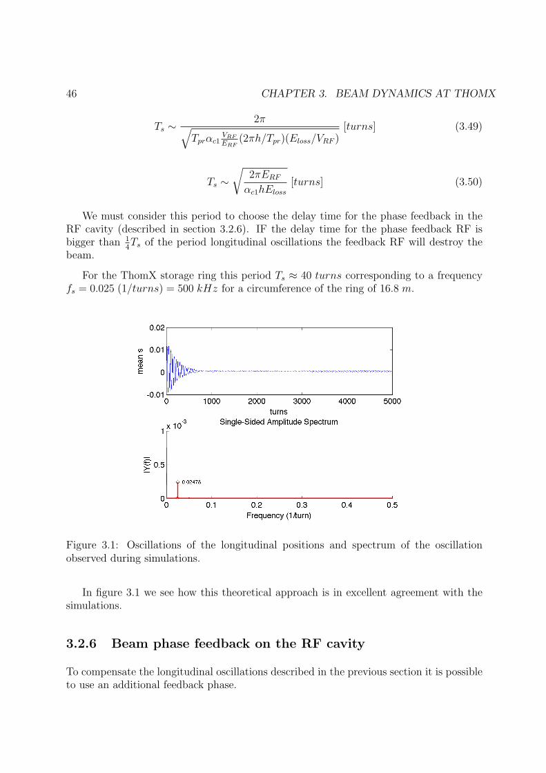
For the ThomX storage ring this period Ts ≈ 40 turns corresponding to a frequencyfs = 0.025 (1/turns) = 500 kHz for a circumference of the ring of 16.8 m.
Figure 3.1: Oscillations of the longitudinal positions and spectrum of the oscillationobserved during simulations.
In figure 3.1 we see how this theoretical approach is in excellent agreement with thesimulations.
3.2.6 Beam phase feedback on the RF cavity
To compensate the longitudinal oscillations described in the previous section it is possibleto use an additional feedback phase.

3.2. LONGITUDINAL DYNAMICS 47
This adds a term φfb,j in equation (3.32):
δEj+1,i = δEj,i +eVRF
ERF
cos(−φs + ωRFSj,i/c+ φfb,j) (3.51)
This phase gives us an amendment for the RF cavity term taking into account real dis-placement of the longitudinal position of the bunch.
φfb,j = −K∗ < Sj−d−1,i > (3.52)
Where d is the feedback delay time expressed in turns, K is a normalizing factor whichequals:
K = Kfbπh/(Tpr ∗ c) (3.53)
The parameter Kfb is the ”gain” of the feedback.
It should be noted that the delay time in the equation (3.52) must agree with theperiod of longitudinal oscillations otherwise there is a risk to get in the opposite phaseand as a consequence to get a resonance that destroy the beam. In figure 3.2 is presentedthe dependence of the amplitude of longitudinal position of the bunch of electrons fromdifferent time delay d in the equation (3.52) of longitudinal phase feedback for ThomX,for Kfb =
1100
.
Figure 3.2: Dependence of the amplitude of the longitudinal position of the bunch ofelectrons from different time delay.
On this plot we can clearly see that even for a such small gain as Kfb =1
100a badly
chosen delay time of feedback system will destroy the bunch quickly. This mean that thedelay time can be in the range of [0 to Ts
4]± nTs (n ∈ N).
48 CHAPTER 3. BEAM DYNAMICS AT THOMX
3.3 Collective effects
The interaction of a beam of charged particles with it is own electromagnetic fields (wakefields) induced in the vacuum beam pipe wall can lead to collective effects and modifythe beam dynamics. The most significant consequence associated with these collectiveeffects is instability of transverse and longitudinal dynamics. If resonance conditionsare achieved a small deviation of beam energy or phase can be amplified by the wakefields. That positive feedback can lead to an increase of the amplitude of the synchrotronoscillations and as consequence reduce the quality of the beam and even destroy the beam.
3.3.1 Wake field formalism
Collective effects can be estimated using the wake field formalism. The normalized integralover the electro-magnetic force (Lorentz force) due to the fields excited by a point charge ordelta function distribution is called the wake function [39]. Wake function is the responsefunction to the excitation by the point charge. In the case of ultra-relativistic bunchesthe wake function is determined only by the form and electro-magnetic parameters of thestructure of the beam pipe.
In this thesis we will look only at longitudinal instabilities produced by collectiveeffects. In such case the wake function can be presented as the integral of the longitudinalcomponent of the E(s) electric field parallel to ~v the speed of the particles.
W (s) = −1
q
∫ ∞
−∞E(s− s′)ds′ (3.54)
Interaction between the wake field and the bunches of charged particle with an arbitrarylongitudinal distribution is defined as wake potential V (s) by a convolution of the wakefunction with the longitudinal charge density n(s) [35]:
V (s) = −∫ ∞
0
W (s− s′)n(s′)ds′ (3.55)
The longitudinal charge density n(s) is normalized as∫∞−∞ n(s)ds = 1.
3.3.2 The longitudinal space charge (LSC)
The longitudinal space charge is a collective effect which occurs from interaction of thecharged particles in the moving bunch with the bunches electromagnetic field (”self-fields”). These ”self-fields” depend on the velocity and the charge of the bunch, geometryand materials of the vacuum beam pipe. Interaction of the bunch with these ”self-fields”

3.3. COLLECTIVE EFFECTS 49
will influence the energy loss, the betatron tunes shift, the synchronous phase and thetune shift, instabilities. In this work we restrict ourselves to the influence of the spacecharge on the energy losses.
Figure 3.3: Scheme LSC
For this we take the longitudinal space charge wake field as defined by A.Chao [35]:
W (s) = −e2√2π(R n(s)− Ldn(s)
ds)
where L = − Z0L0
4πcγ2 (2 ln(b/a) + 1), a = 12(σx + σy), σx,y is the transverse size of the
bunch, b = γσs, σs is the longitudinal size of the bunch, γ is the relativistic factor, R isthe resistivity and L is the inductivity of the vacuum pipe wall, Z0 = 4π/c ≈ 377 Ω is theimpedance of free space.
The influence of the longitudinal space charge wake field on the beam dynamics ispresented on page 67.
3.3.3 Resistive Wall (RW)
Resistive Wall instability comes from the electrons in the bunch inducing currents on thebeam pipe wall. Due to the finite resistivity of the walls, these currents extend behind theposition of the relativistic electrons bunch. The electro-magnetic fields of this currentsacts on the particle arriving later and may increase their oscillation amplitudes, energydeviation...
To take into account RW wake field we use the short-range wake fields assuming aconstant conductivity [40] we obtain as:
W (s) = −e∫∞−∞ E(s− s′)n(s′)ds
50 CHAPTER 3. BEAM DYNAMICS AT THOMX
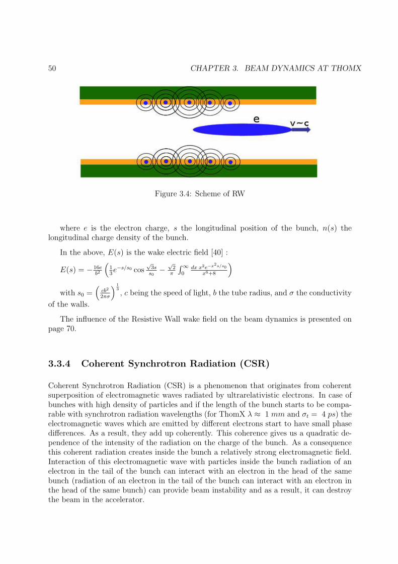
Figure 3.4: Scheme of RW
where e is the electron charge, s the longitudinal position of the bunch, n(s) thelongitudinal charge density of the bunch.
In the above, E(s) is the wake electric field [40] :
E(s) = −16eb2
(
13e−s/s0 cos
√3ss0
−√2
π
∫∞0
dx x2e−x2s/s0
x6+8
)
with s0 =(
cb2
2πσ
) 13, c being the speed of light, b the tube radius, and σ the conductivity
of the walls.
The influence of the Resistive Wall wake field on the beam dynamics is presented onpage 70.
3.3.4 Coherent Synchrotron Radiation (CSR)
Coherent Synchrotron Radiation (CSR) is a phenomenon that originates from coherentsuperposition of electromagnetic waves radiated by ultrarelativistic electrons. In case ofbunches with high density of particles and if the length of the bunch starts to be compa-rable with synchrotron radiation wavelengths (for ThomX λ ≈ 1 mm and σt = 4 ps) theelectromagnetic waves which are emitted by different electrons start to have small phasedifferences. As a result, they add up coherently. This coherence gives us a quadratic de-pendence of the intensity of the radiation on the charge of the bunch. As a consequencethis coherent radiation creates inside the bunch a relatively strong electromagnetic field.Interaction of this electromagnetic wave with particles inside the bunch radiation of anelectron in the tail of the bunch can interact with an electron in the head of the samebunch (radiation of an electron in the tail of the bunch can interact with an electron inthe head of the same bunch) can provide beam instability and as a result, it can destroythe beam in the accelerator.

3.3. COLLECTIVE EFFECTS 51
Figure 3.5: Scheme CSR
The interaction of the electrons with their own electromagnetic field is taken intoaccount with terms composed of two parts [41] :
Vcsr sh(s) = Vcrs free−space + Vshielded (3.56)
Vcrs free−space is the term that accounts for the wake field of CSR for the free-spaceterm when an electron bunch is circulating along a circular trajectory [42]:
Vcrs free−space = −2πR
4πǫ0eNe
(∫ ∞
0
1
(3R2)1/3dn(s− s′)
ds
1
(s′)1/3ds′
)
(3.57)
Where R is the bending magnet radius, ǫ0 is the vacuum permittivity.
Vshielded is the term that accounts for the shielded effect induced by the beam pipe. Inthe approach proposed in [43] the beam pipe is represented by two infinite parallel platesseparated by a height 2h. In this case we have
Vshielded(s) =2πR
4πǫ0eNe
(
1
2h2
∫ +∞
−∞n(s− s′)G2
[
1
2h2
(
R
h
)1/2
s′
]
ds′
)
(3.58)
where G2 is the scaling functions defined by J.B. MURPHY et al [43], equation 5.22b.
The influence of CSR wake field on beam dynamics is presented on page 70.
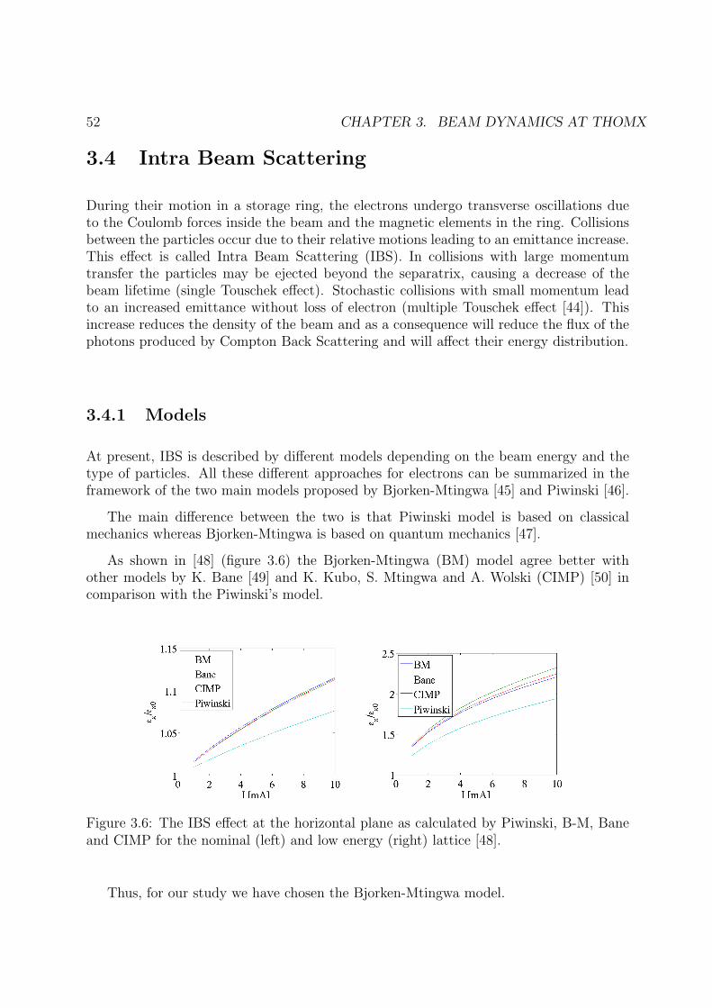
52 CHAPTER 3. BEAM DYNAMICS AT THOMX
3.4 Intra Beam Scattering
During their motion in a storage ring, the electrons undergo transverse oscillations dueto the Coulomb forces inside the beam and the magnetic elements in the ring. Collisionsbetween the particles occur due to their relative motions leading to an emittance increase.This effect is called Intra Beam Scattering (IBS). In collisions with large momentumtransfer the particles may be ejected beyond the separatrix, causing a decrease of thebeam lifetime (single Touschek effect). Stochastic collisions with small momentum leadto an increased emittance without loss of electron (multiple Touschek effect [44]). Thisincrease reduces the density of the beam and as a consequence will reduce the flux of thephotons produced by Compton Back Scattering and will affect their energy distribution.
3.4.1 Models
At present, IBS is described by different models depending on the beam energy and thetype of particles. All these different approaches for electrons can be summarized in theframework of the two main models proposed by Bjorken-Mtingwa [45] and Piwinski [46].
The main difference between the two is that Piwinski model is based on classicalmechanics whereas Bjorken-Mtingwa is based on quantum mechanics [47].
As shown in [48] (figure 3.6) the Bjorken-Mtingwa (BM) model agree better withother models by K. Bane [49] and K. Kubo, S. Mtingwa and A. Wolski (CIMP) [50] incomparison with the Piwinski’s model.
Figure 3.6: The IBS effect at the horizontal plane as calculated by Piwinski, B-M, Baneand CIMP for the nominal (left) and low energy (right) lattice [48].
Thus, for our study we have chosen the Bjorken-Mtingwa model.
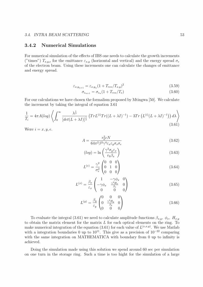
3.4. INTRA BEAM SCATTERING 53
3.4.2 Numerical Simulations
For numerical simulation of the effects of IBS one needs to calculate the growth increments(”times”) Tx,y,e for the emittance εx,y (horizontal and vertical) and the energy spread σe
of the electron beam. Using these increments one can calculate the changes of emittanceand energy spread.
εx,yn+1= εx,yn(1 + Trev/Tx,y)
2 (3.59)
σen+1 = σen(1 + Trev/Te) (3.60)
For our calculations we have chosen the formalism proposed by Mtingwa [50]. We calculatethe increment by taking the integral of equation 3.61
1
Ti
= 4πA(log)
⟨
∫ ∞
0
λ12
[det(L+ λI)]12
(
TrL(i)Tr((L+ λI)−1)− 3Tr(
L(i)(L+ λI)−1))
dλ
⟩
(3.61)Were i = x, y, e.
A =r20cN
64π2β3γ4εxεyσsσe
(3.62)
(log) = ln
(
γ2σyεxr0βx
)
(3.63)
L(e) =γ2
σ2e
0 0 00 1 00 0 0
(3.64)
L(x) =βx
εx
1 −γφx 0
−γφxγ2Hx
βx0
0 0 0
(3.65)
L(y) =βy
εy
0 0 0
0 γ2Hy
βy0
0 0 0
(3.66)
To evaluate the integral (3.61) we need to calculate amplitude functions βx,y, φx, Hx,y
to obtain the matrix element for the matrix L for each optical elements on the ring. Tomake numerical integration of the equation (3.61) for each value of L(e,x,y). We use Matlabwith a integration boundaries 0 up to 1011. This give as a precision of 10−22 comparingwith the same integration on MATHEMATICA with boundary from 0 up to infinity isachieved.
Doing the simulation made using this solution we spend around 60 sec per simulationon one turn in the storage ring. Such a time is too hight for the simulation of a large

54 CHAPTER 3. BEAM DYNAMICS AT THOMX
number of turns. We noticed that the contribution of the IBS effect give almost a linearincrease of the emittance and energy spread over small ranges. To reduce the calculationtime we use the following strategy: we use the values of the growth increments (seeequation 3.59) calculated on a previous turn. The integration of the IBS equation 3.61is done only when the difference for energy spread calculated during the last calculationand the current value is greater than a set value. This method give us good accuracy andsaves time for the simulations.
Next what we try to get a better accuracy for IBS. By using some linear extrapolationsfor the calculations of growth increments (see equation 3.59):
Ti,n = Ti,n−1 +Ti,nl − Ti,nlp
nl − nlp(3.67)
Were i = p, x, y are longitudinal and transverse coordinates, n is the number of currentturn, nl is the number of turn since IBS has calculated (evaluate the integral 3.61), nlp isthe number of turns when was calculated IBS before nl. Also we notice that the changesgiven in energy spread during IBS is considerably smaller than those from LongitudinalDynamics. So we decided to change the conditions under which we will recalculate IBS(evaluate the integral 3.61). We make it in several steps. First step if condition 3.68 isvalid it means that the contribution of IBS effects is 100 time smaller than other.
∆σe,n < |σe,n − σe,n−1|/100 (3.68)
In this case we don’t need to calculate IBS again. Also we check:
|σe,nl − σe,n|/σe,n > 5 ∗ 10−2 (3.69)
In case of changes of energy spread greater than 5% IBS will calculated. Next step ischecking changes on emittance.
|εx,nl − εx,n|/εx,n > 10−2 (3.70)
If the change of emittance during the last calculations of IBS is more than 1% we recal-culate (evaluate the integral 3.61) IBS.
As we can see from figure 3.7 we receive a good agreement between method of cal-culating IBS with using or without using approximation. Accordingly we can use theextrapolations to get a result close to reality and save a factor 10 − 100 in the durationof simulations.
At this point it is important to notice that the effect of IBS is strongly dependent fromthe parameters of the bunch such as geometrical size of the bunch and energy distributions.For bunch with smaller sizes the effect of IBS will be bigger and for bunch with biggersizes the effect of IBS will be smaller. This dependence is illustrated in figure 3.8 fordifferent initial bunch length.This give an understanding that during simulations of IBS
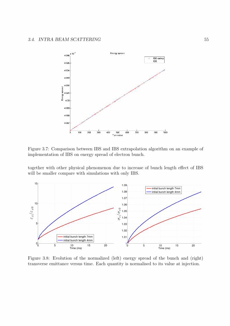
3.4. INTRA BEAM SCATTERING 55
Figure 3.7: Comparison between IBS and IBS extrapolation algorithm on an example ofimplementation of IBS on energy spread of electron bunch.
together with other physical phenomenon due to increase of bunch length effect of IBSwill be smaller compare with simulations with only IBS.
0 5 10 15 200
5
10
15
Time (ms)
εx/εx0
initial bunch length 7mm
initial bunch length 4mm
0 5 10 15 201
1.01
1.02
1.03
1.04
1.05
1.06
1.07
1.08
1.09
Time (ms)
σe/σe0
initial bunch length 7mm
initial bunch length 4mm
Figure 3.8: Evolution of the normalized (left) energy spread of the bunch and (right)transverse emittance versus time. Each quantity is normalised to its value at injection.

56 CHAPTER 3. BEAM DYNAMICS AT THOMX
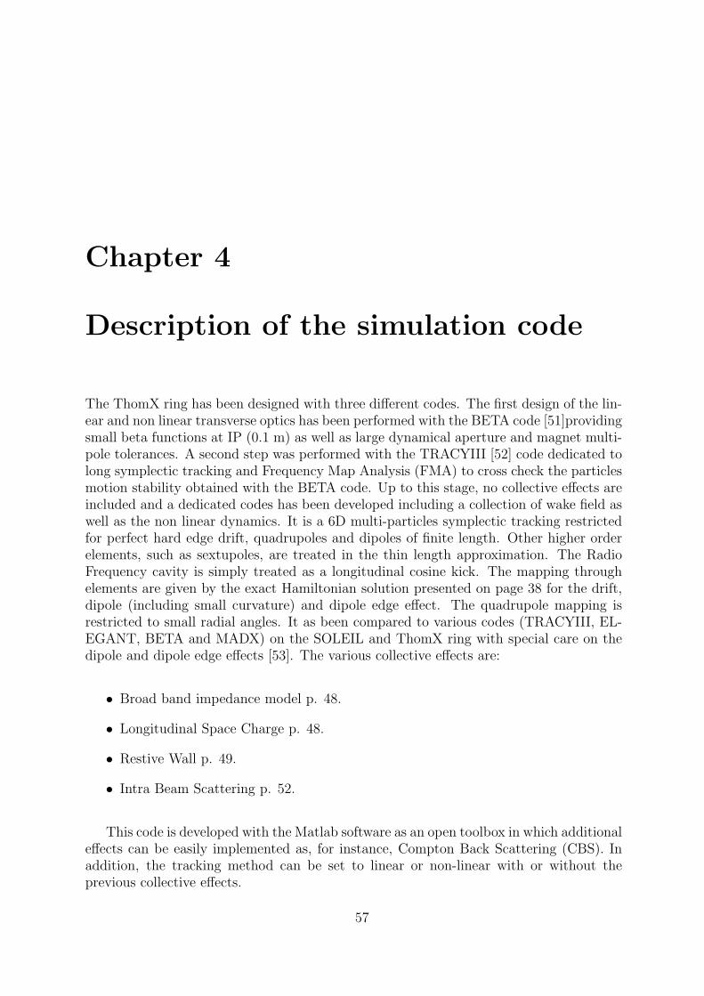
Chapter 4
Description of the simulation code
The ThomX ring has been designed with three different codes. The first design of the lin-ear and non linear transverse optics has been performed with the BETA code [51]providingsmall beta functions at IP (0.1 m) as well as large dynamical aperture and magnet multi-pole tolerances. A second step was performed with the TRACYIII [52] code dedicated tolong symplectic tracking and Frequency Map Analysis (FMA) to cross check the particlesmotion stability obtained with the BETA code. Up to this stage, no collective effects areincluded and a dedicated codes has been developed including a collection of wake field aswell as the non linear dynamics. It is a 6D multi-particles symplectic tracking restrictedfor perfect hard edge drift, quadrupoles and dipoles of finite length. Other higher orderelements, such as sextupoles, are treated in the thin length approximation. The RadioFrequency cavity is simply treated as a longitudinal cosine kick. The mapping throughelements are given by the exact Hamiltonian solution presented on page 38 for the drift,dipole (including small curvature) and dipole edge effect. The quadrupole mapping isrestricted to small radial angles. It as been compared to various codes (TRACYIII, EL-EGANT, BETA and MADX) on the SOLEIL and ThomX ring with special care on thedipole and dipole edge effects [53]. The various collective effects are:
• Broad band impedance model p. 48.
• Longitudinal Space Charge p. 48.
• Restive Wall p. 49.
• Intra Beam Scattering p. 52.
This code is developed with the Matlab software as an open toolbox in which additionaleffects can be easily implemented as, for instance, Compton Back Scattering (CBS). Inaddition, the tracking method can be set to linear or non-linear with or without theprevious collective effects.
57

58 CHAPTER 4. DESCRIPTION OF THE SIMULATION CODE
4.1 Architecture
To achieve this task the programming language MATLAB was chosen. The code can besplit on 2 main parts:
• A starting shell in which the beam profile is prepared or loaded.
• A main loop inside which the processes occurring during one turn of the electronbeam in the ThomX ring will be simulate.
The principal scheme of the starting shell is presented in Figure 4.1:
In the starting shell we set the initial parameters of the simulations, both physical andlocal. Physical parameters contain information about of the electron bunch at injection,the laser pulse and the parameters of the accelerator ring. Local parameters contain flagsto select the type and length in number of turns of the simulation and the path to loadthe initial data and save the final data of simulation. Important feature of the startingshell is to save all informations at the end of the simulation to have the possibility to runthe next simulation exactly at the place where the previous simulation was finished. Thisgives the possibility to be independent from the limit of the computational time duringsimulations of a large number of turns. Also starting the shell can run several simulationswith different parameters values for electron beam and laser pulse and for the acceleratorring. This open the possibility to scan for different regime at injection, study the influenceof errors in misalignment of synchronisation of the electron bunch and the laser pulse atthe interaction point of the Compton scattering and many other things.
4.2 Performance
The Main loop simulates the beam propagation through the accelerator ring during oneturn with the selected physical phenomena. The scheme of the main loop is presented onFigure 4.2.
The flags specified in the starting shell select the type of simulation. The followingflags are implemented in the code:
• rflags.IBS; simulate IBS
• rflags.CBS; simulate CBS
• rflags.track bunch LIN ; simulate linear bunch propagation
• rflags.track bunch wake; simulate non linear bunch propagation

4.2. PERFORMANCE 59
Each of them can be set to either 0 (NO) or 1 (Y ES).
If rflags.track bunch LIN = 1 linear beam propagation of the beam through trans-port matrices of the accelerator and propagation through the RF cavity will be simulated.
If rflags.track bunch wake = 1 non linear beam propagation of the beam using theHamiltonian formalism will be simulated taking into account non linear effects and sim-ulating propagation through RF cavity with longitudinal phase feedback taking into ac-count delay time. In starting shell a protection is added which does not allow rflags.track bunch LINand rflags.track bunch wake to be set at the same time. In this non linear simulationwe can add additional flags to simulate the collective effects:
• rflags.LSC wake; simulate LSC
• rflags.RW wake; simulate RW
• rflags.CSR shielded wake; simulate CSR
Collective effects can be simulated all together or separately to study each effect morein detail.
Each flag can run the function to calculate the wake-field for the corresponding col-lective effect. These wake-field are represented by a kick applied to the bunch at differentlocations along the ring.
If rflags.IBS = 1 the growth time due to Intra Beam Scattering averaged around thering and the corresponding emittance increment added to bunch will be calculated.
If rflags.CBS = 1 it will a run function to modify the 6-D phase space to 14-Dbeam profile used by the CAIN code and run the code CAIN to simulate Compton BackScattering of the electron bunch with the laser pulse. After CAIN finishes the simulationthe 14-D beam profile will be transformed back into the 6-D phase-space. Profile ofscattered photons will be saved in the output directory.
After each of theses functions a checking function is called to verify if a particle wentout of the acceptance of the accelerator. Particles which go out of acceptance are deletedfrom the bunch.

60 CHAPTER 4. DESCRIPTION OF THE SIMULATION CODE
Figure 4.1: The structure of the initial part of the code.

4.2. PERFORMANCE 61
Figure 4.2: Structure of the main loop.

62 CHAPTER 4. DESCRIPTION OF THE SIMULATION CODE

Chapter 5
Results of the simulations and theirinterpretation
5.1 Linear tracking
To study the beam dynamics in ThomX it is important to do simulations of linear trackingof the electron beam through the accelerator ring. To minimize the oscillations due tomismatching in the longitudinal plane between bunch length and energy spread, we usethe formula 5.1 proposed in [54] to match the bunch length to the energy.
σs
2=
c|ηc|Ω
σe (5.1)
were Ω the synchrotron frequency and ηc is the momentum compaction. Using thisexpression we can obtain a matched bunch length σs = 0.007 m and energy spreadσs = 0.3% for ThomX.
As we can see from the figure 5.1, injecting a matched beam and simulating lineartracking has perfect beam evolution during all injection cycle (20 ms). As we can seethe amplitude of the synchrotron oscillations is around of 10−18 which can be assumedas 0 due to rounding errors during matrix multiplications and limited number of macroparticles in the bunch.
Unfortunately injecting a matched beam in ThomX is not possible. Technical param-eters of the gun, the linear accelerator and the injection section will inject in the ring abunch with a banana shape as profile in the longitudinal phase space as shown in figure5.2.
Injecting a non matched bunch with a banana shape profile and using linear trackingwe clearly see in figure 5.3 that now we have large amplitude of synchrotron oscillationsfor phase and energy spread.
63

64CHAPTER 5. RESULTS OF THE SIMULATIONS AND THEIR INTERPRETATION
−0.5 0 0.5 1
x 10−14
−5
−4
−3
−2
−1
0
1
2
3
4
5x 10
−18
longitudinal phase [deg]
me
an
re
lative
en
erg
y d
E/E
0
0 0.01 0.02
−0.5
0
0.5
x 10−14
ph
ase
[d
eg
]
0 0.01 0.02−5
0
5x 10
−18
me
an
re
lative
en
erg
y d
E/E
0
time [s]
Figure 5.1: Evolution on phase space matched beam during linear tracking 20 ms or400000 turns.
Figure 5.2: Initial longitudinal beam profile of the bunch non matched banana shape(left) and matched beam (right).
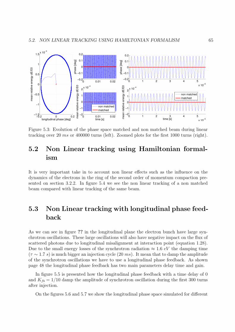
5.2. NON LINEAR TRACKING USING HAMILTONIAN FORMALISM 65
−0.2 0 0.2−1.5
−1
−0.5
0
0.5
1
1.5x 10
−4
longitudinal phase [deg]
mean r
ela
tive e
nerg
y d
E/E
0
0 0.01 0.02−0.2
−0.1
0
0.1
0.2
phase [deg]
0 0.01 0.02−2
−1
0
1
2x 10
−4
mean r
ela
tive e
nerg
y d
E/E
0
time [s]
non matched
matched
0 1 2 3 4 5
x 10−5
−0.2
−0.1
0
0.1
0.2
phase [deg]
0 1 2 3 4 5
x 10−5
−2
−1
0
1
2x 10
−4
mean r
ela
tive e
nerg
y d
E/E
0
time [s]
non matched
matched
Figure 5.3: Evolution of the phase space matched and non matched beam during lineartracking over 20 ms or 400000 turns (left). Zoomed plots for the first 1000 turns (right).
5.2 Non Linear tracking using Hamiltonian formal-
ism
It is very important take in to account non linear effects such as the influence on thedynamics of the electrons in the ring of the second order of momentum compaction pre-sented on section 3.2.2. In figure 5.4 we see the non linear tracking of a non matchedbeam compared with linear tracking of the same beam.
5.3 Non Linear tracking with longitudinal phase feed-
back
As we can see in figure ?? in the longitudinal plane the electron bunch have large syn-chrotron oscillations. These large oscillations will also have negative impact on the flux ofscattered photons due to longitudinal misalignment at interaction point (equation 1.28).Due to the small energy losses of the synchrotron radiation ≈ 1.6 eV the damping time(τ ∼ 1.7 s) is much bigger an injection cycle (20 ms). It mean that to damp the amplitudeof the synchrotron oscillations we have to use a longitudinal phase feedback. As shownpage 48 the longitudinal phase feedback has two main parameters delay time and gain.
In figure 5.5 is presented how the longitudinal phase feedback with a time delay of 0and Kfb = 1/10 damp the amplitude of synchrotron oscillation during the first 300 turnsafter injection.
On the figures 5.6 and 5.7 we show the longitudinal phase space simulated for different
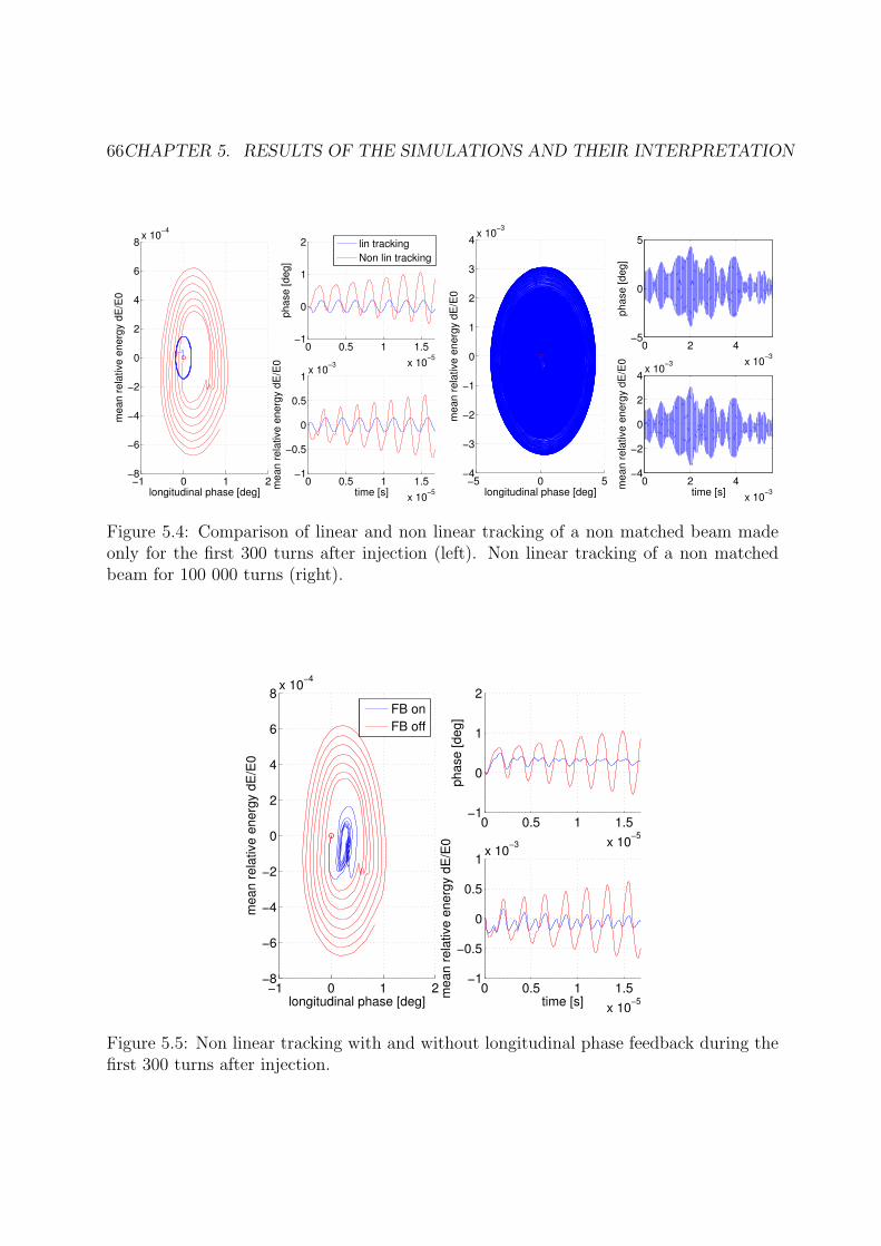
66CHAPTER 5. RESULTS OF THE SIMULATIONS AND THEIR INTERPRETATION
−1 0 1 2−8
−6
−4
−2
0
2
4
6
8x 10
−4
longitudinal phase [deg]
me
an
re
lative
en
erg
y d
E/E
0
0 0.5 1 1.5
x 10−5
−1
0
1
2
ph
ase
[d
eg
]
lin tracking
Non lin tracking
0 0.5 1 1.5
x 10−5
−1
−0.5
0
0.5
1x 10
−3
me
an
re
lative
en
erg
y d
E/E
0
time [s]−5 0 5
−4
−3
−2
−1
0
1
2
3
4x 10
−3
longitudinal phase [deg]
mean r
ela
tive e
nerg
y d
E/E
0
0 2 4
x 10−3
−5
0
5
phase [deg]
0 2 4
x 10−3
−4
−2
0
2
4x 10
−3
mean r
ela
tive e
nerg
y d
E/E
0
time [s]
Figure 5.4: Comparison of linear and non linear tracking of a non matched beam madeonly for the first 300 turns after injection (left). Non linear tracking of a non matchedbeam for 100 000 turns (right).
−1 0 1 2−8
−6
−4
−2
0
2
4
6
8x 10
−4
longitudinal phase [deg]
me
an
re
lative
en
erg
y d
E/E
0
FB on
FB off
0 0.5 1 1.5
x 10−5
−1
0
1
2
ph
ase
[d
eg
]
0 0.5 1 1.5
x 10−5
−1
−0.5
0
0.5
1x 10
−3
me
an
re
lative
en
erg
y d
E/E
0
time [s]
Figure 5.5: Non linear tracking with and without longitudinal phase feedback during thefirst 300 turns after injection.

5.4. NON LINEAR TRACKING WITH LONGITUDINAL SPACE CHARGE 67
values of feedback time delay made for 10000 turns.
−2 0 2 4−2
−1.5
−1
−0.5
0
0.5
1
1.5x 10
−3
longitudinal phase [deg]
mean r
ela
tive e
nerg
y d
E/E
0
0 2 4
x 10−4
−2
−1
0
1
2
phase [deg]
0 2 4
x 10−4
−1
0
1
x 10−3
mean r
ela
tive e
nerg
y d
E/E
0
time [s]−0.5 0 0.5 1−5
−4
−3
−2
−1
0
1
2
3
4
5x 10
−4
longitudinal phase [deg]
mean r
ela
tive e
nerg
y d
E/E
0
0 2 4
x 10−4
−2
−1
0
1
2
phase [deg]
0 2 4
x 10−4
−1
0
1
x 10−3
mean r
ela
tive e
nerg
y d
E/E
0
time [s]
Figure 5.6: Non linear tracking without longitudinal phase feedback (left). Non lineartracking with longitudinal phase feedback for feedback with no time delay, correspondingto a perfect feedback model (right).
As we can see on this figure 5.7 for a feedback time delay of 9 turns the longitudinalfeedback ceases to operate and the reason of that is now correction in phase occurs at thewrong phase of synchrotron oscillation at as 1/4 of period it (see section 3.2.6).
On next the figure presented result of simulation made for feedback time delay =41 turns and as we can see longitudinal phase feedback works well for this time delay.Therefore it is possible to use electronics for a feedback system with a time of reaction≈ 2 µs.
5.4 Non Linear tracking with Longitudinal Space Charge
In figure 5.9 simulations with and without Longitudinal Space Charge (LSC) are pre-sented.
As we can see due to the Longitudinal Space Charge the wake field of the beamexplodes and get to a stable regime only after loosing macroparticle that go outside theenergy acceptance.
To reduce this negative influence of Longitudinal Space Charge wake field on the beamwe can use longitudinal phase feedback (FB). In figure 5.10 are presented simulations oftracking with Longitudinal Space Charge wake field with longitudinal phase feedback(FB) and without.
As we can see from these simulations presented in figure 5.10 the longitudinal phase
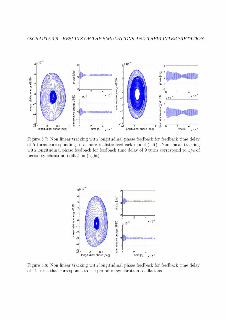
68CHAPTER 5. RESULTS OF THE SIMULATIONS AND THEIR INTERPRETATION
−0.5 0 0.5 1−6
−4
−2
0
2
4
6x 10
−4
longitudinal phase [deg]
mean r
ela
tive e
nerg
y d
E/E
0
0 2 4
x 10−4
−2
−1
0
1
2
phase [deg]
0 2 4
x 10−4
−1
0
1
x 10−3
mean r
ela
tive e
nerg
y d
E/E
0
time [s]−1 0 1 2
−10
−8
−6
−4
−2
0
2
4
6
8x 10
−4
longitudinal phase [deg]
me
an
re
lative
en
erg
y d
E/E
0
0 2 4
x 10−4
−2
−1
0
1
2
ph
ase
[d
eg
]
0 2 4
x 10−4
−1
0
1
x 10−3
me
an
re
lative
en
erg
y d
E/E
0
time [s]
Figure 5.7: Non linear tracking with longitudinal phase feedback for feedback time delayof 5 turns corresponding to a more realistic feedback model (left). Non linear trackingwith longitudinal phase feedback for feedback time delay of 9 turns correspond to 1/4 ofperiod synchrotron oscillation (right).
−0.5 0 0.5 1−5
−4
−3
−2
−1
0
1
2
3
4
5x 10
−4
longitudinal phase [deg]
mean r
ela
tive e
nerg
y d
E/E
0
0 2 4
x 10−4
−2
−1
0
1
2
phase [deg]
0 2 4
x 10−4
−1
0
1
x 10−3
mean r
ela
tive e
nerg
y d
E/E
0
time [s]
Figure 5.8: Non linear tracking with longitudinal phase feedback for feedback time delayof 41 turns that corresponds to the period of synchrotron oscillations.

5.4. NON LINEAR TRACKING WITH LONGITUDINAL SPACE CHARGE 69
0 1 2 3 4 50
1
2
3
4
5
6
7
8
9x 10
−3
Time (ms)
std
energ
y s
pre
ad
FB 0 tb w 1 LSC w 1 RW w 0
FB 0 tb w 1 LSC w 0 RW w 0
0 1 2 3 4 5−10
−8
−6
−4
−2
0
2
4
6
8x 10
−3
Time (ms)
me
an
en
erg
y
FB 0 tb w 1 LSC w 1 RW w 0
FB 0 tb w 1 LSC w 0 RW w 0
Figure 5.9: Evolution of (left) energy spread of the bunch and (right) position of energybarycentre of the bunch. Blue line is simulation with LSC and red without LSC.
0 1 2 3 4 50
1
2
3
4
5
6
7
8
9x 10
−3
Time (ms)
std
energ
y s
pre
ad
FB 0 tb w 1 LSC w 1 RW w 0
FB 1 tb w 1 LSC w 1 RW w 0
0 1 2 3 4 5−10
−8
−6
−4
−2
0
2
4
6
8x 10
−3
Time (ms)
me
an
en
erg
y
FB 0 tb w 1 LSC w 1 RW w 0
FB 1 tb w 1 LSC w 1 RW w 0
Figure 5.10: Evolution of (left) energy spread of the bunch and (right) position of energybarycentre of the bunch. Blue line is simulation with FB and red without FB.
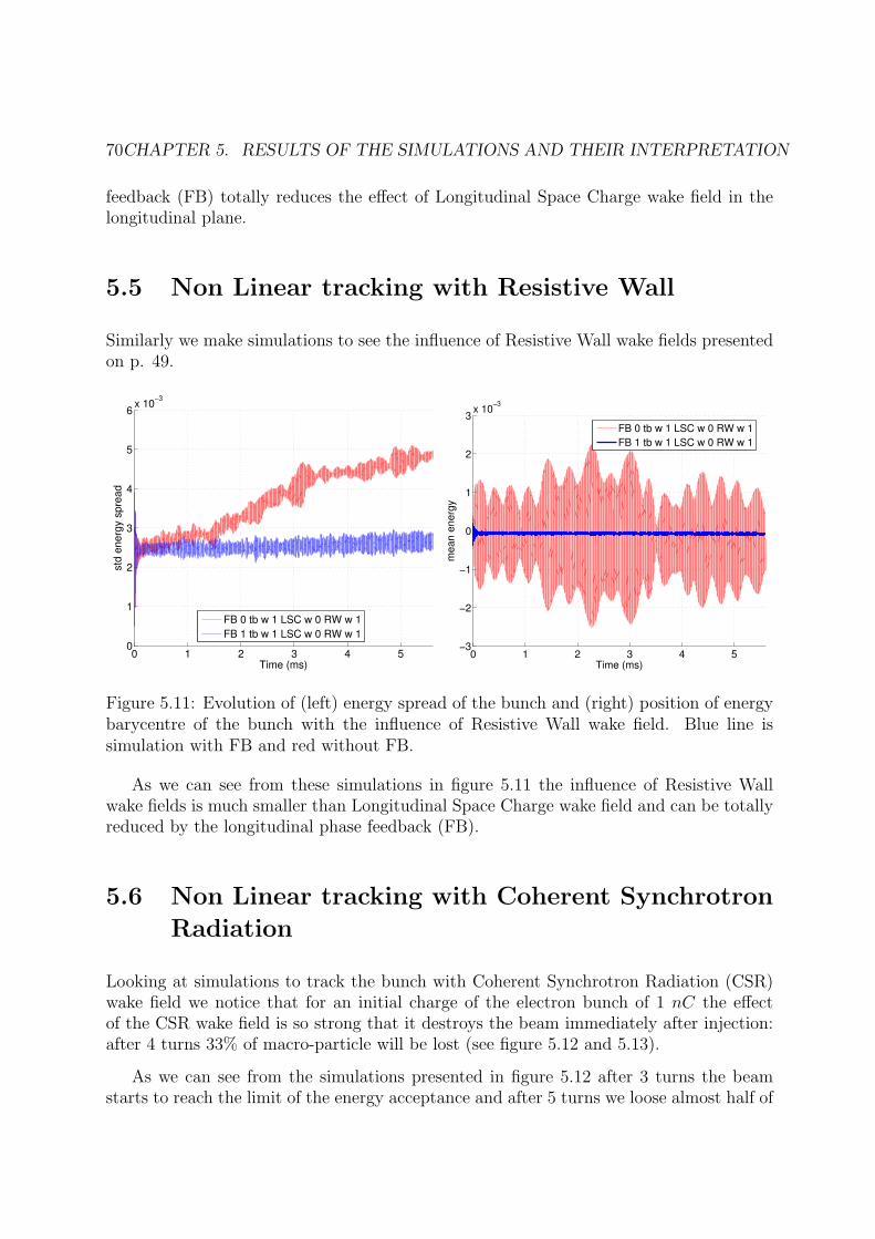
70CHAPTER 5. RESULTS OF THE SIMULATIONS AND THEIR INTERPRETATION
feedback (FB) totally reduces the effect of Longitudinal Space Charge wake field in thelongitudinal plane.
5.5 Non Linear tracking with Resistive Wall
Similarly we make simulations to see the influence of Resistive Wall wake fields presentedon p. 49.
0 1 2 3 4 50
1
2
3
4
5
6x 10
−3
Time (ms)
std
energ
y s
pre
ad
FB 0 tb w 1 LSC w 0 RW w 1
FB 1 tb w 1 LSC w 0 RW w 1
0 1 2 3 4 5−3
−2
−1
0
1
2
3x 10
−3
Time (ms)
me
an
en
erg
y
FB 0 tb w 1 LSC w 0 RW w 1
FB 1 tb w 1 LSC w 0 RW w 1
Figure 5.11: Evolution of (left) energy spread of the bunch and (right) position of energybarycentre of the bunch with the influence of Resistive Wall wake field. Blue line issimulation with FB and red without FB.
As we can see from these simulations in figure 5.11 the influence of Resistive Wallwake fields is much smaller than Longitudinal Space Charge wake field and can be totallyreduced by the longitudinal phase feedback (FB).
5.6 Non Linear tracking with Coherent Synchrotron
Radiation
Looking at simulations to track the bunch with Coherent Synchrotron Radiation (CSR)wake field we notice that for an initial charge of the electron bunch of 1 nC the effectof the CSR wake field is so strong that it destroys the beam immediately after injection:after 4 turns 33% of macro-particle will be lost (see figure 5.12 and 5.13).
As we can see from the simulations presented in figure 5.12 after 3 turns the beamstarts to reach the limit of the energy acceptance and after 5 turns we loose almost half of

5.6. NON LINEAR TRACKING WITH COHERENT SYNCHROTRON RADIATION 71
Figure 5.12: Evolution of the longitudinal phase space under the influence of Coherentsynchrotron radiation (CSR) wake field.
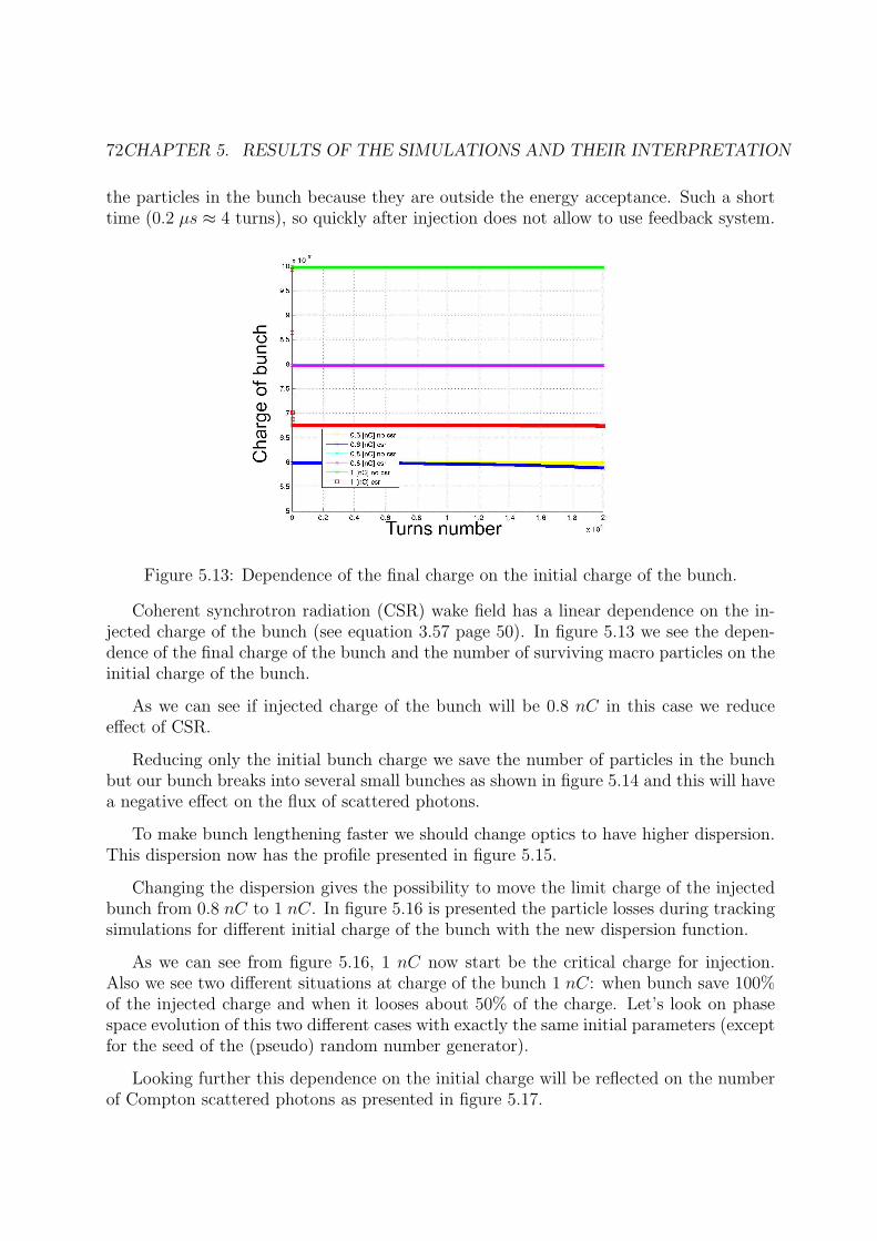
72CHAPTER 5. RESULTS OF THE SIMULATIONS AND THEIR INTERPRETATION
the particles in the bunch because they are outside the energy acceptance. Such a shorttime (0.2 µs ≈ 4 turns), so quickly after injection does not allow to use feedback system.
Figure 5.13: Dependence of the final charge on the initial charge of the bunch.
Coherent synchrotron radiation (CSR) wake field has a linear dependence on the in-jected charge of the bunch (see equation 3.57 page 50). In figure 5.13 we see the depen-dence of the final charge of the bunch and the number of surviving macro particles on theinitial charge of the bunch.
As we can see if injected charge of the bunch will be 0.8 nC in this case we reduceeffect of CSR.
Reducing only the initial bunch charge we save the number of particles in the bunchbut our bunch breaks into several small bunches as shown in figure 5.14 and this will havea negative effect on the flux of scattered photons.
To make bunch lengthening faster we should change optics to have higher dispersion.This dispersion now has the profile presented in figure 5.15.
Changing the dispersion gives the possibility to move the limit charge of the injectedbunch from 0.8 nC to 1 nC. In figure 5.16 is presented the particle losses during trackingsimulations for different initial charge of the bunch with the new dispersion function.
As we can see from figure 5.16, 1 nC now start be the critical charge for injection.Also we see two different situations at charge of the bunch 1 nC: when bunch save 100%of the injected charge and when it looses about 50% of the charge. Let’s look on phasespace evolution of this two different cases with exactly the same initial parameters (exceptfor the seed of the (pseudo) random number generator).
Looking further this dependence on the initial charge will be reflected on the numberof Compton scattered photons as presented in figure 5.17.
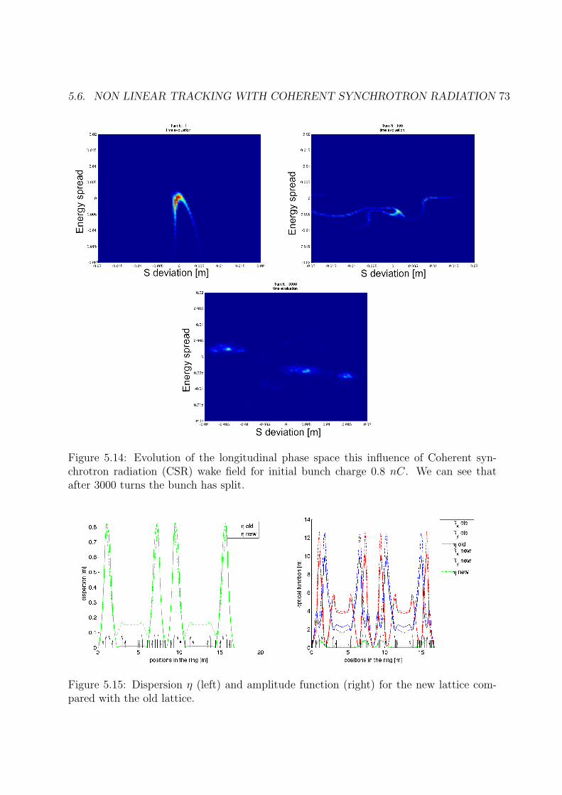
5.6. NON LINEAR TRACKING WITH COHERENT SYNCHROTRON RADIATION 73
Figure 5.14: Evolution of the longitudinal phase space this influence of Coherent syn-chrotron radiation (CSR) wake field for initial bunch charge 0.8 nC. We can see thatafter 3000 turns the bunch has split.
Figure 5.15: Dispersion η (left) and amplitude function (right) for the new lattice com-pared with the old lattice.
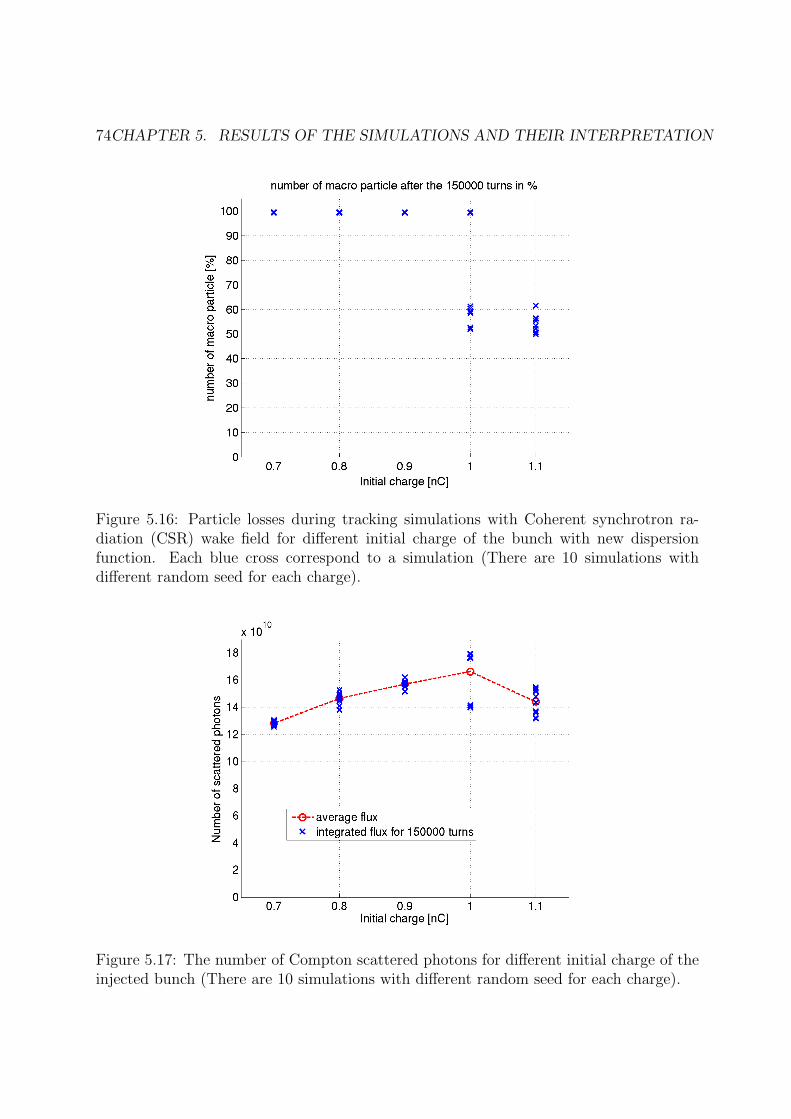
74CHAPTER 5. RESULTS OF THE SIMULATIONS AND THEIR INTERPRETATION
Figure 5.16: Particle losses during tracking simulations with Coherent synchrotron ra-diation (CSR) wake field for different initial charge of the bunch with new dispersionfunction. Each blue cross correspond to a simulation (There are 10 simulations withdifferent random seed for each charge).
Figure 5.17: The number of Compton scattered photons for different initial charge of theinjected bunch (There are 10 simulations with different random seed for each charge).

5.6. NON LINEAR TRACKING WITH COHERENT SYNCHROTRON RADIATION 75
Figure 5.18: Evolutions of longitudinal phase space. Left is for CSR without beam breakup and losses. Right is for CSR with beam break up leading to losses.
The beam break up seen in figure 5.18 leads to large amplitude oscillations of thebarycentre of the bunch, leading to losses of ∼ 50% of the electrons in the bunch. We cansee these from the bump in figure 5.21, 5.22 at around 1.1 ms . The split bunch increasesso much that one of the parts goes out of the acceptance.
Figure 5.19 and 5.21 present the evolution of the mean energy spread and phase ofthe beam for the simulations presented in figure 5.18.
Changing the lattice gives the possibility to increase the limit charge for the injectedbunch but does not reduce the problem of the bunch break up.To reduce this destructiveeffect of CSR wake field as shown in figure 5.16 one must reduce the initial charge ofbunch. But as we can see from figure 5.17 and from equation 1.28 reducing the charge ofinjected bunch of electrons we also reduce the flux of scattered photons due to Comptonback scattering.
Another way is to operate the injection with a different setting: apply an energy offsetto the electrons to compensate the first turns CSR losses by running the linac slightlyoff-crest in order to fix the bunch lengthening and to mitigate the CSR risks. The lastmethod gives us the possibility to damp the amplitude of the oscillations and to mitigatethe destructive effects of CSR.
To simulate the energy offset we simply add a constant value to the energy spread of
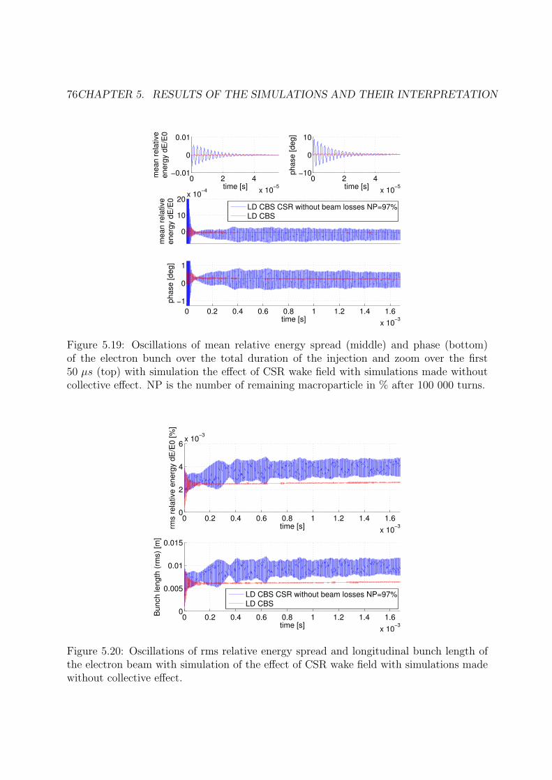
76CHAPTER 5. RESULTS OF THE SIMULATIONS AND THEIR INTERPRETATION
0 2 4
x 10−5
−0.01
0
0.01
me
an
re
lative
en
erg
y d
E/E
0
time [s]0 2 4
x 10−5
−10
0
10
ph
ase
[d
eg
]
time [s]
0
10
20x 10
−4
me
an
re
lative
en
erg
y d
E/E
0
LD CBS CSR without beam losses NP=97%
LD CBS
0 0.2 0.4 0.6 0.8 1 1.2 1.4 1.6
x 10−3
−1
0
1
ph
ase
[d
eg
]
time [s]
Figure 5.19: Oscillations of mean relative energy spread (middle) and phase (bottom)of the electron bunch over the total duration of the injection and zoom over the first50 µs (top) with simulation the effect of CSR wake field with simulations made withoutcollective effect. NP is the number of remaining macroparticle in % after 100 000 turns.
0 0.2 0.4 0.6 0.8 1 1.2 1.4 1.6
x 10−3
0
2
4
6x 10
−3
rms r
ela
tive e
nerg
y d
E/E
0 [%
]
time [s]
0 0.2 0.4 0.6 0.8 1 1.2 1.4 1.6
x 10−3
0
0.005
0.01
0.015
time [s]
Bunch length
(rm
s)
[m]
LD CBS CSR without beam losses NP=97%
LD CBS
Figure 5.20: Oscillations of rms relative energy spread and longitudinal bunch length ofthe electron beam with simulation of the effect of CSR wake field with simulations madewithout collective effect.
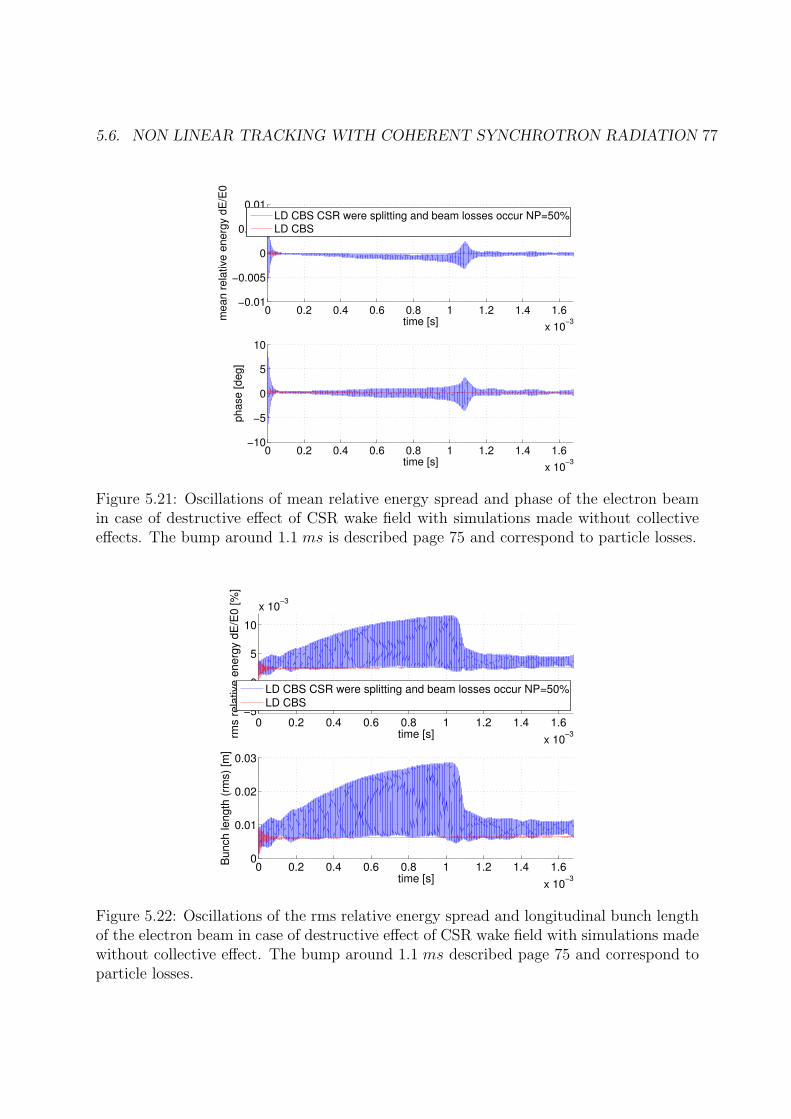
5.6. NON LINEAR TRACKING WITH COHERENT SYNCHROTRON RADIATION 77
0 0.2 0.4 0.6 0.8 1 1.2 1.4 1.6
x 10−3
−0.01
−0.005
0
0.005
0.01
me
an
re
lative
en
erg
y d
E/E
0
time [s]
LD CBS CSR were splitting and beam losses occur NP=50%
LD CBS
0 0.2 0.4 0.6 0.8 1 1.2 1.4 1.6
x 10−3
−10
−5
0
5
10
ph
ase
[d
eg
]
time [s]
Figure 5.21: Oscillations of mean relative energy spread and phase of the electron beamin case of destructive effect of CSR wake field with simulations made without collectiveeffects. The bump around 1.1 ms is described page 75 and correspond to particle losses.
0 0.2 0.4 0.6 0.8 1 1.2 1.4 1.6
x 10−3
−5
0
5
10
x 10−3
rms r
ela
tive
en
erg
y d
E/E
0 [
%]
time [s]
LD CBS CSR were splitting and beam losses occur NP=50%
LD CBS
0 0.2 0.4 0.6 0.8 1 1.2 1.4 1.6
x 10−3
0
0.01
0.02
0.03
Bu
nch
le
ng
th (
rms)
[m]
time [s]
Figure 5.22: Oscillations of the rms relative energy spread and longitudinal bunch lengthof the electron beam in case of destructive effect of CSR wake field with simulations madewithout collective effect. The bump around 1.1 ms described page 75 and correspond toparticle losses.
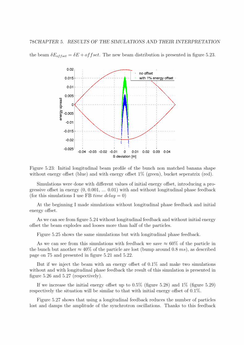
78CHAPTER 5. RESULTS OF THE SIMULATIONS AND THEIR INTERPRETATION
the beam δEoffset = δE + offset. The new beam distribution is presented in figure 5.23.
Figure 5.23: Initial longitudinal beam profile of the bunch non matched banana shapewithout energy offset (blue) and with energy offset 1% (green), bucket seperatrix (red).
Simulations were done with different values of initial energy offset, introducing a pro-gressive offset in energy (0, 0.001, ... 0.01) with and without longitudinal phase feedback(for this simulations I use FB time delay = 0)
At the beginning I made simulations without longitudinal phase feedback and initialenergy offset.
As we can see from figure 5.24 without longitudinal feedback and without initial energyoffset the beam explodes and looses more than half of the particles.
Figure 5.25 shows the same simulations but with longitudinal phase feedback.
As we can see from this simulations with feedback we save ≈ 60% of the particle inthe bunch but another ≈ 40% of the particle are lost (bump around 0.8 ms), as describedpage on 75 and presented in figure 5.21 and 5.22.
But if we inject the beam with an energy offset of 0.1% and make two simulationswithout and with longitudinal phase feedback the result of this simulation is presented infigure 5.26 and 5.27 (respectively).
If we increase the initial energy offset up to 0.5% (figure 5.28) and 1% (figure 5.29)respectively the situation will be similar to that with initial energy offset of 0.1%.
Figure 5.27 shows that using a longitudinal feedback reduces the number of particleslost and damps the amplitude of the synchrotron oscillations. Thanks to this feedback

5.6. NON LINEAR TRACKING WITH COHERENT SYNCHROTRON RADIATION 79
Figure 5.24: Evolution of the phase space (left) and phase space of the bunch (rightup) with longitudinal particle distribution (right down) after 20000 turns made duringsimulation without feedback and initial energy offset.
Figure 5.25: Evolution phase space (left) and phase space of the bunch (right up) withlongitudinal particle distribution (right down) after 20000 turns made during simulationwith feedback but without initial energy offset.
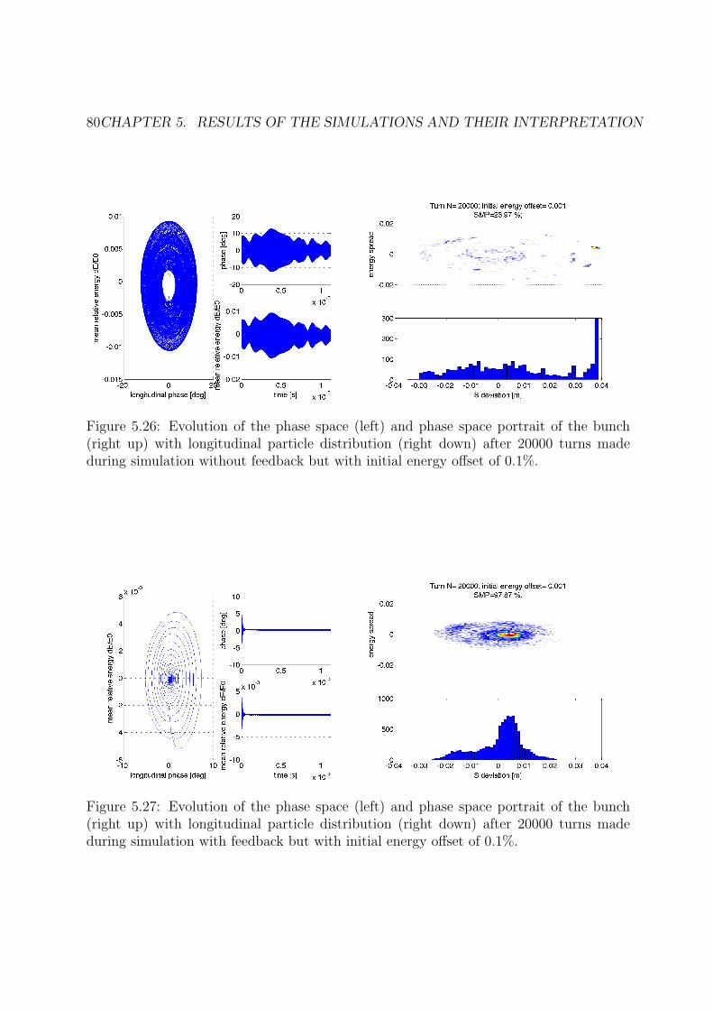
80CHAPTER 5. RESULTS OF THE SIMULATIONS AND THEIR INTERPRETATION
Figure 5.26: Evolution of the phase space (left) and phase space portrait of the bunch(right up) with longitudinal particle distribution (right down) after 20000 turns madeduring simulation without feedback but with initial energy offset of 0.1%.
Figure 5.27: Evolution of the phase space (left) and phase space portrait of the bunch(right up) with longitudinal particle distribution (right down) after 20000 turns madeduring simulation with feedback but with initial energy offset of 0.1%.
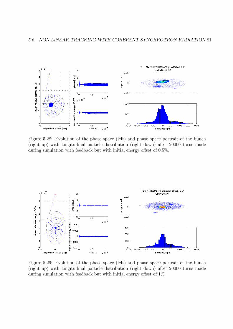
5.6. NON LINEAR TRACKING WITH COHERENT SYNCHROTRON RADIATION 81
Figure 5.28: Evolution of the phase space (left) and phase space portrait of the bunch(right up) with longitudinal particle distribution (right down) after 20000 turns madeduring simulation with feedback but with initial energy offset of 0.5%.
Figure 5.29: Evolution of the phase space (left) and phase space portrait of the bunch(right up) with longitudinal particle distribution (right down) after 20000 turns madeduring simulation with feedback but with initial energy offset of 1%.
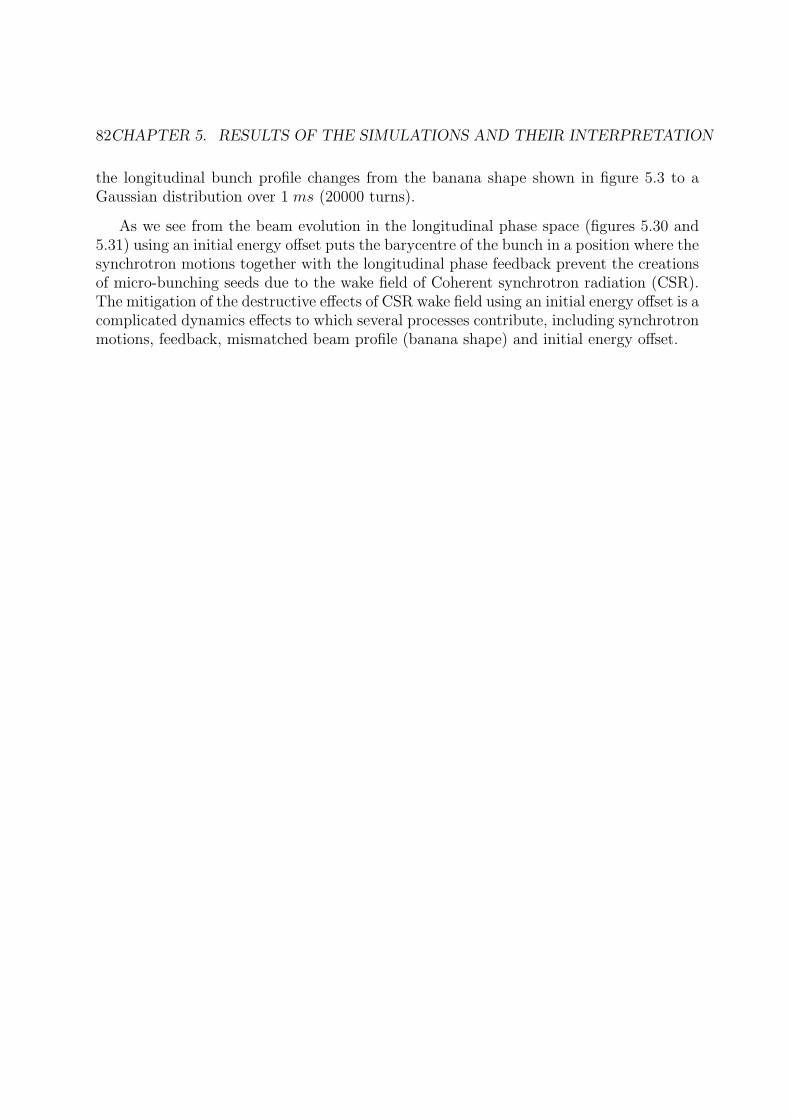
82CHAPTER 5. RESULTS OF THE SIMULATIONS AND THEIR INTERPRETATION
the longitudinal bunch profile changes from the banana shape shown in figure 5.3 to aGaussian distribution over 1 ms (20000 turns).
As we see from the beam evolution in the longitudinal phase space (figures 5.30 and5.31) using an initial energy offset puts the barycentre of the bunch in a position where thesynchrotron motions together with the longitudinal phase feedback prevent the creationsof micro-bunching seeds due to the wake field of Coherent synchrotron radiation (CSR).The mitigation of the destructive effects of CSR wake field using an initial energy offset is acomplicated dynamics effects to which several processes contribute, including synchrotronmotions, feedback, mismatched beam profile (banana shape) and initial energy offset.

5.6. NON LINEAR TRACKING WITH COHERENT SYNCHROTRON RADIATION 83
Figure 5.30: Evolution of the longitudinal phase space under the influence of Coherentsynchrotron radiation (CSR) wake field with (blue) initial energy offset of 1% and without(red) with longitudinal phase feedback.

84CHAPTER 5. RESULTS OF THE SIMULATIONS AND THEIR INTERPRETATION
Figure 5.31: Evolution of the longitudinal phase space under the influence of Coherentsynchrotron radiation (CSR) wake field with (blue) initial energy offset of 1% and without(red) with longitudinal phase feedback.

5.7. SIMULATION OF THE EFFECT OF INTRA BEAM SCATTERING 85
5.7 Simulation of the effect of Intra Beam Scattering
To understand the effect of Intra beam scattering on the flux of scattered photons I madethree simulations with the same initial bunch distribution (matched beam) and simulatedthe linear tracking with:
• Compton Back Scattering (CBS).
• Intra Beam Scattering (IBS).
• Intra Beam Scattering and Compton Back Scattering (IBS+CBS).
With these simulations we can compare the influence of IBS and CBS on the beamdynamics under linear tracking.
0 5 10 15 201
1.05
1.1
1.15
1.2
1.25
1.3
1.35
1.4
Time (ms)
σe/σe0
IBS+CBS
IBS
CBS
0 5 10 15 201
1.5
2
2.5
3
3.5
4
4.5
5
Time (ms)
εx/εx0
IBS+CBS
IBS
CBS
Figure 5.32: Evolution of the normalized (left) energy spread of the bunch and (right)transverse emittance versus time. Each quantity is normalised to its value at injection.
As we can see for the evolution of the relative energy spread, CBS is dominant whereasfor the horizontal emittance the dominant effect is IBS.
We have seen in formula 1.27 that the flux of scattered photons is inversely proportionalto the beam size. As due to IBS the transverse size of the bunch increases (see figure5.33) the flux will decrease. The evolution of the flux of scattered photons is presented infigure 5.34.
But Intra Beam Scattering changes not only the geometrical sizes of the electron bunchbut it also increases the energy spread of the particles in the longitudinal plane and thehorizontal plane. As a result the energy distributions will be changed also. Figure 5.34shows the energy spectrum of the scattered photons for simulations with and without
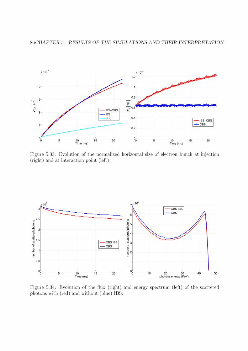
86CHAPTER 5. RESULTS OF THE SIMULATIONS AND THEIR INTERPRETATION
0 5 10 15 206
7
8
9
10
x 10−4
Time (ms)
σx[m
]
IBS+CBS
IBS
CBS
0 5 10 15 200
0.2
0.4
0.6
0.8
1
1.2
x 10−4
σx[m
]
Time (ms)
IBS+CBS
CBS
Figure 5.33: Evolution of the normalized horizontal size of electron bunch at injection(right) and at interaction point (left)
0 5 10 15 200
0.5
1
1.5
2
2.5
3
x 109
num
ber
of scattere
d p
hoto
ns
Time (ms)
CBS IBS
CBS
0 10 20 30 40 500
1
2
3
4
5
6
7x 10
9
nu
mb
er
of
sca
tte
red
ph
oto
ns
photons energy (KeV)
CBS IBS
CBS
Figure 5.34: Evolution of the flux (right) and energy spectrum (left) of the scatteredphotons with (red) and without (blue) IBS.

5.7. SIMULATION OF THE EFFECT OF INTRA BEAM SCATTERING 87
Intra Beam Scattering. On this figure 5.34 we can see the influence of IBS on the flux ofscattered photons.
To see influence of increases of the horizontal emittance on the energy distributionof scattered photons due to IBS we look at the distribution of the number of scatteredphotons versus energy spectrum to the angle of scattering.
Figure 5.35: Distribution of the scattered photons,energy spectrum versus angle of scat-tering made in the case with IBS (left) and without (right).
It is hard to see that the spectrum made with IBS has a broader profile. To see thisdifference clearly we slice this distribution by angular bin of 0.3 mrad and we calculatethe full width half maximum of each slice in the energy plane (figure 5.36). This highlightsthe different width of the two energy spectrum.
Also to see this difference we can see if we normalise the distribution of scatteredphotons versus the energy spectrum to the angle of scattering on the number of scatteredphotons and subtract one distributions from another as presented in figure 5.37.
On this figure 5.37 now we clearly can see that the distribution of the scattered photonswith IBS has a wider width (red) and that without IBS the scattered photons have asharper distribution in energy spectrum. Now we can clearly see that the effect of IBShas some influence on the energy spectrum of the scattered photons and some influenceon the flux of scattered photons (see figure 5.34).

88CHAPTER 5. RESULTS OF THE SIMULATIONS AND THEIR INTERPRETATION
−15 −10 −5 0 5 10 150
1
2
3
4
5
6
7
angle (mrad)
Sp
ectr
um
FW
HM
(K
eV
)
estm=0.5
CBS IBS
CBS
Figure 5.36: Full width half maximum of the energy spectrum of angular slices of width0.3 mrad of the scattered photons with IBS (red) and without IBS (blue).
angle (mrad)
ph
oto
ns e
ne
rgy (
Ke
V)
Diff with IBS − without IBS
−15 −10 −5 0 5 10 155
10
15
20
25
30
35
40
45
50
−0.2
−0.15
−0.1
−0.05
0
0.05
0.1
0.15
0.2
Figure 5.37: Difference of normalised distribution of scattered photons, energy spectrumversus angle of scattering.

5.8. COMPARISONOF THE EFFECTOF ALL THE PROCESSES ON THE COMPTON FLUX89
5.8 Comparison of the effect of all the processes on
the Compton flux
I made simulations of all physical effects included in the code and studied how they changethe beam dynamics and as consequence how they affect the flux and energy distributionsof scattered photons. I made simulations with all these effects together to see how theywill affect the beam simultaneously and modify the influence of each other.
For this we make two set of simulations one without longitudinal feedback (FB 0 EnOf 0)and another with longitudinal feedback and with an initial energy offset of 1% (FB 1 EnOf 1).The last one give us the possibility to remove the destructive effect of CSR seen in theprevious chapter.
All these simulations were done with the ”banana shape” distributions of the electronbunch and non linear 6-D bunch tracking.
Figure 5.38 shows that the influence of IBS on the flux of scattered photons will bereduced when it is considered together with non linear 6-D tracking. This is due to theincrease of emittance and energy spread with this process.
When LSC is added to the simulations presented in figure 5.39 we clearly see the effectof longitudinal feedback (FB) that does not give the possibility to the LSC wake field toincrease the energy spread and reduce the amplitude of the oscillations mean energy asshown in figure 5.10. The difference of flux at the beginning is explained by the initialincrease of the horizontal emittance due to the initial energy offset.
The effect of RW is presented in figure 5.40. It will also be reduced by the longitudinalFB, but compared with the LSC influence of the RW on the beam dynamics is muchsmaller and in this case we see a big effect on the flux due to the initial energy offset.
But as shown in the chapter about of CSR (see page 70) an initial energy offset isnecessary to reduce the destructive effect of CSR and we can see it on the evolution ofthe number of macro particles in the bunch in figure 5.42. This influence of the initialenergy offset on the beam dynamics together with longitudinal FB is presented in figure5.41.
The factors that cause this difference in flux in figure 5.41 are the loss of electronsdue to CSR and the different positions of the centre of mass for the electrons withoutlongitudinal feedback as presented in figure 5.42.
The initial energy offset will lead to an increase of transverse size of the bunch andtherefore a reduced a flux. However this energy offset mitigates the destructive effect ofCSR leading to less electron losses and more stable bunch position and delivers higherflux.
From the simulation presented in figure 5.43 we can clearly see that for the ThomXring the dominating physical phenomena which provide the biggest beam losses and as

90CHAPTER 5. RESULTS OF THE SIMULATIONS AND THEIR INTERPRETATION
0 5 10 15 200
1
2
x 1010
Time (ms)
Flu
x [
ph
oto
ns/m
s]
IBS 1 FB 0 EnOf 0 LSC 0 RW 0 CSR 0; Flux=3.9e+11
IBS 0 FB 0 EnOf 0 LSC 0 RW 0 CSR 0; Flux=3.9e+11
IBS 1 FB 1 EnOf 1 LSC 0 RW 0 CSR 0; Flux=3.6e+11
IBS 0 FB 1 EnOf 1 LSC 0 RW 0 CSR 0; Flux=3.7e+11
0 10 200
2
4
6x 10
−7
Time (ms)
εxm
rad
0 10 200
2
4
6x 10
−3
Time (ms)
std
en
erg
y s
pre
ad
Figure 5.38: Effect of IBS. Evolution of the flux (top), of the horizontal emittance of theelectron bunch (left bottom), of the energy spread of the electron bunch (right bottom).Simulations without longitudinal feedback (FB 0 EnOf 0; red and blue) and with lon-gitudinal feedback and with initial energy offset 1% (FB 1 EnOf 1; magenta and cyan),with IBS (red and magenta) and without (blue and cyan)

5.8. COMPARISONOF THE EFFECTOF ALL THE PROCESSES ON THE COMPTON FLUX91
0 5 10 15 200
1
2
x 1010
Time (ms)
Flu
x [
ph
oto
ns/m
s]
IBS 0 FB 0 EnOf 0 LSC 0 RW 0 CSR 0; Flux=3.9e+11
IBS 0 FB 0 EnOf 0 LSC 1 RW 0 CSR 0; Flux=3.4e+11
IBS 0 FB 1 EnOf 1 LSC 1 RW 0 CSR 0; Flux=4.2e+11
0 10 200
2
4
6x 10
−7
Time (ms)
εxm
rad
0 10 200
0.005
0.01
Time (ms)
std
en
erg
y s
pre
ad
Figure 5.39: Effect of LSC. Evolution of the flux (top), of the horizontal emittance ofthe electron bunch (left bottom) and of the energy spread of the electron bunch (rightbottom)
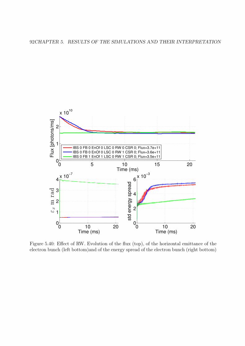
92CHAPTER 5. RESULTS OF THE SIMULATIONS AND THEIR INTERPRETATION
0 5 10 15 200
1
2
x 1010
Time (ms)
Flu
x [
ph
oto
ns/m
s]
IBS 0 FB 0 EnOf 0 LSC 0 RW 0 CSR 0; Flux=3.7e+11
IBS 0 FB 0 EnOf 0 LSC 0 RW 1 CSR 0; Flux=3.6e+11
IBS 0 FB 1 EnOf 1 LSC 0 RW 1 CSR 0; Flux=3.5e+11
0 10 200
1
2
3
4x 10
−7
Time (ms)
εxm
rad
0 10 200
2
4
6x 10
−3
Time (ms)
std
en
erg
y s
pre
ad
Figure 5.40: Effect of RW. Evolution of the flux (top), of the horizontal emittance of theelectron bunch (left bottom)and of the energy spread of the electron bunch (right bottom)

5.8. COMPARISONOF THE EFFECTOF ALL THE PROCESSES ON THE COMPTON FLUX93
0 5 10 15 200
1
2
x 1010
Time (ms)
Flu
x [
ph
oto
ns/m
s]
IBS 0 FB 0 EnOf 0 LSC 0 RW 0 CSR 0; Flux=3.9e+11
IBS 0 FB 0 EnOf 0 LSC 0 RW 0 CSR 1; Flux=2.8e+11
IBS 0 FB 1 EnOf 1 LSC 0 RW 0 CSR 1; Flux=3.9e+11
0 10 200
1
2
3x 10
−7
Time (ms)
εxm
rad
0 10 200
0.005
0.01
0.015
Time (ms)
std
en
erg
y s
pre
ad
Figure 5.41: Effect of CSR. Evolution of the flux (top). Evolution of the horizontalemittance of the electron bunch (left bottom). Evolution of the energy spread of theelectron bunch (right bottom)

94CHAPTER 5. RESULTS OF THE SIMULATIONS AND THEIR INTERPRETATION
0 5 10 15 200
1000
2000
3000
4000
5000
6000
7000
8000
9000
10000
Nu
mb
er
of
ma
cro
ele
ctr
on
s
Time (ms)
IBS 1 FB 0 EnOf 0 LSC 1 RW 1 CSR 1
IBS 1 FB 1 EnOf 1 LSC 1 RW 1 CSR 1
0 5 10 15 200
0.5
1
1.5
x 10−4
Std
X [m
]
Time (ms)0 5 10 15 20
−5
−4
−3
−2
−1
0
1
2
3
4
5x 10
−5
Mean X
[m
]
Time (ms)
0 5 10 15 200
0.005
0.01
0.015
0.02
Std
S [
m]
Time (ms)0 5 10 15 20
−0.02
−0.015
−0.01
−0.005
0
0.005
0.01
0.015
0.02
Mean S
[m
]
Time (ms)
Figure 5.42: Evolution of the number of particle in the bunch (top), of the horizontalsize of the electron bunch (left center), of the horizontal position of the barycentre of theelectron bunch (right center), of longitudinal size of the electron bunch (right bottom)and of the longitudinal position of the barycentre of the electron bunch (right bottom).
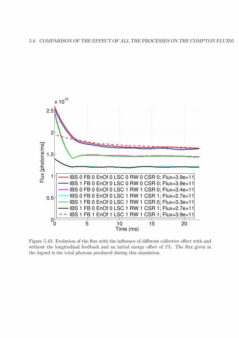
5.8. COMPARISONOF THE EFFECTOF ALL THE PROCESSES ON THE COMPTON FLUX95
0 5 10 15 200
0.5
1
1.5
2
2.5
x 1010
Time (ms)
Flu
x [photo
ns/m
s]
IBS 0 FB 0 EnOf 0 LSC 0 RW 0 CSR 0; Flux=3.9e+11IBS 1 FB 0 EnOf 0 LSC 0 RW 0 CSR 0; Flux=3.9e+11IBS 0 FB 0 EnOf 0 LSC 1 RW 1 CSR 0; Flux=3.4e+11IBS 0 FB 0 EnOf 0 LSC 1 RW 1 CSR 1; Flux=2.7e+11IBS 1 FB 0 EnOf 0 LSC 1 RW 1 CSR 0; Flux=3.3e+11IBS 1 FB 0 EnOf 0 LSC 1 RW 1 CSR 1; Flux=2.7e+11IBS 1 FB 1 EnOf 1 LSC 1 RW 1 CSR 1; Flux=3.9e+11
Figure 5.43: Evolution of the flux with the influence of different collective effect with andwithout the longitudinal feedback and an initial energy offset of 1%. The flux given inthe legend is the total photons produced during this simulation.

96CHAPTER 5. RESULTS OF THE SIMULATIONS AND THEIR INTERPRETATION
consequence reduce the flux of scattered photons is CSR.
The effect of the method I have proposed to mitigate the effect of CSR is shown infigure 5.41. By implementing longitudinal FB and injecting the beam with an initialenergy offset the flux of scattered photons is improved by 33%.
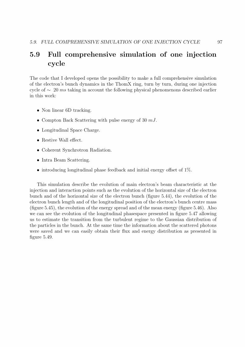
5.9. FULL COMPREHENSIVE SIMULATION OF ONE INJECTION CYCLE 97
5.9 Full comprehensive simulation of one injection
cycle
The code that I developed opens the possibility to make a full comprehensive simulationof the electron’s bunch dynamics in the ThomX ring, turn by turn, during one injectioncycle of ∼ 20 ms taking in account the following physical phenomenons described earlierin this work:
• Non linear 6D tracking.
• Compton Back Scattering with pulse energy of 30 mJ .
• Longitudinal Space Charge.
• Restive Wall effect.
• Coherent Synchrotron Radiation.
• Intra Beam Scattering.
• introducing longitudinal phase feedback and initial energy offset of 1%.
This simulation describe the evolution of main electron’s beam characteristic at theinjection and interaction points such as the evolution of the horizontal size of the electronbunch and of the horizontal size of the electron bunch (figure 5.44), the evolution of theelectron bunch length and of the longitudinal position of the electron’s bunch centre mass(figure 5.45), the evolution of the energy spread and of the mean energy (figure 5.46). Alsowe can see the evolution of the longitudinal phasespace presented in figure 5.47 allowingus to estimate the transition from the turbulent regime to the Gaussian distribution ofthe particles in the bunch. At the same time the information about the scattered photonswere saved and we can easily obtain their flux and energy distribution as presented infigure 5.49.
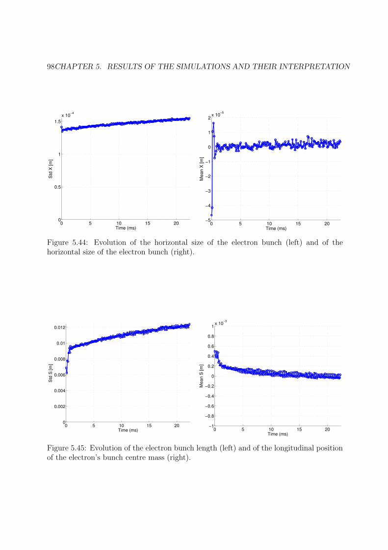
98CHAPTER 5. RESULTS OF THE SIMULATIONS AND THEIR INTERPRETATION
0 5 10 15 200
0.5
1
1.5
x 10−4
Std
X [m
]
Time (ms)0 5 10 15 20
−5
−4
−3
−2
−1
0
1
2x 10
−5
Me
an
X [
m]
Time (ms)
Figure 5.44: Evolution of the horizontal size of the electron bunch (left) and of thehorizontal size of the electron bunch (right).
0 5 10 15 200
0.002
0.004
0.006
0.008
0.01
0.012
Std
S [
m]
Time (ms) 0 5 10 15 20−1
−0.8
−0.6
−0.4
−0.2
0
0.2
0.4
0.6
0.8
1x 10
−3
Mean S
[m
]
Time (ms)
Figure 5.45: Evolution of the electron bunch length (left) and of the longitudinal positionof the electron’s bunch centre mass (right).

5.9. FULL COMPREHENSIVE SIMULATION OF ONE INJECTION CYCLE 99
0 5 10 15 200
0.5
1
1.5
2
2.5
3
3.5
4
4.5
5x 10
−3
std
rela
tive e
nerg
y
Time (ms)
0 5 10 15 20−1
−0.8
−0.6
−0.4
−0.2
0
0.2
0.4
0.6
0.8
1x 10
−3
mean r
ela
tive e
nerg
y
Time (ms)
Figure 5.46: Evolution of the energy spread (left) and of the mean energy (right).
Figure 5.47: Evolution of the longitudinal phasespace.

100CHAPTER 5. RESULTS OF THE SIMULATIONS AND THEIR INTERPRETATION
0 5 10 15 200
0.2
0.4
0.6
0.8
1
1.2
1.4
1.6
1.8
2x 10
10
Flu
x [
ph
oto
ns/m
s]
Time (ms)
Figure 5.48: Evolution of the flux (left) and energy distribution of scattered photons(right).
0 10 20 30 40 500
1
2
3
4
5
6
7x 10
8
nu
mb
er
of
sca
tte
red
ph
oto
ns
photons energy (KeV)
First 10000 turns
Last 10000 turns
Figure 5.49: Comparison of the energy spectrum of the scattered photons for the flux ofthe first 10000 turns after injection and of 10000 turns after 240000 turns.

Chapter 6
Conclusion
In this document I presented my work on transverse and longitudinal non linear dynamicsof an electron beam in a Compton X-ray source storage ring.
This is important in the framework of the ThomX project, a novel X-ray source basedon Compton backscattering. ThomX is a compact electron storage ring and the beamdynamics studies of the machine parameters I did will allow the electron beam to meetthe high quality requirements at the point of collision with the laser photons.
I investigated the influence of the electrons’ beam parameters on the flux and theenergy distribution of the Compton photons. I also studied the influence of misalignmentsand synchronisation errors on this flux.
To achieve this I worked an a code that takes into account the main physics factors ofa beam dynamics like Compton recoil, intrabeam scattering and Touscheck effect.
Thanks to this code I found a strong influence of non linear effects and non matchedinjection on the beam dynamics.
I presented the possibility to apply a longitudinal feedback and the effect of the feed-back’s delay in the simulation to explore its damping effect and a direct RF feedback. Inthis context I took part in measurement and analysis of the RF cavity for ThomX.
I also introduced collective effects such as longitudinal space charge, resistive wall andcoherent synchrotron radiation that affect the beam in the accelerator.
This allows having a full 6D simulation of the beam dynamics in a Compton ringtaking into account the feedback stabilisation for the 400 000 turns (∼ 20 ms) of oneinjection cycle.
This code has the important feature of combining 6D non linear tracking with collectiveeffects, longitudinal phase feedback, intrabeam scattering and Compton backscattering inthe same simulation. This simulation code can be run on a computer farm.
101

102 CHAPTER 6. CONCLUSION
Intra Beam Scattering is one of the most calculation intensive process but I imple-mented a simplified method that reduces the computation time by a factor 100 withoutsignificant increases in uncertainties.
I checked that the effects of intrabeam scattering is very strong at the injection dueto the short bunch length and small transverse emittances and its effect become smallerwith growing beam size. I also showed that the effect of intrabeam scattering on theenergy distributions of the scattered photons is caused by the increase of the transversemomentum of the electron bunch.
I verified that the negative impact of some collective effects such as longitudinal spacecharge and resistive wall and injection mismatch can be attenuated by the implementationof a longitudinal phase feedback.
I found that the effect of coherent synchrotron radiation is dominating the beamdynamics due to very the short bunch length at the injection.
I present a strategy to reduce the destructive and disruptive influence of coherentsynchrotron radiation by the using longitudinal feedback together with an initial linacenergy offset.
In the future the code I developed and these simulations will help the operators ofThomX to have a good understanding of the beam dynamics, especially during its com-missioning phase due to start in 2015.
Bibliography
[1] H. Motz, “Applications of the radiation from fast electron beams”, Journal ofApply Physics 22 (1951) no. 527, 527–531.
[2] K. Landecker, “Possibility of frequency multiplication and wave amplification bymeans of some relativistic effects”, Phys. Rev. 86 (1952) no. 6, .
[3] R. H. Milburn, “Electron scattering by an intense polarized photon field”, Phys.Rev. Lett. 10 (1963) no. 3, 75–77.
[4] The Great Soviet Encyclopedia. 3rd edition ed., 1970-1979.
[5] J. Dik, K. Janssens, G. Van Der Snickt, L. van der Loeff, K. Rickers, and M. Cotte,“Visualization of a lost painting by vincent van gogh using synchrotron radiationbased x-ray fluorescence elemental mapping”, Analytical Chemistry 80 (2008)no. 16, 6436–6442.
[6] H. G. J. Moseley, “The high frequency spectra of the elements”, Phil. Mag (1913)1024.
[7] A. Revenko, “X-ray spectral fluorescence analysis of natural materials”, Nauka(1994) 264.
[8] P. Verhovodov, “X-ray analysis. differential account of physical processes.”, Kiev:Naukova Dumka (1992) 235.
[9] M. Blokhin, The physics of X-rays. U. S. Atomic Energy Commission, Office ofTechnical Information, 1957.
[10] M. Ando and C. Uyama., Medical Applications of Synchrotron Radiation. Springer,1998.
[11] P. Suortti and W. Thomlinson, “Medical applications of synchrotron radiation”,Physics in Medicine and Biology 48 (2003) no. 13, R1.
[12] E. Rubenstein, E. B. Hughes, L. E. Campbell, R. Hofstadter, R. L. Kirk, T. J.Krolicki, J. P. Stone, S. Wilson, H. D. Zeman, W. R. Brody, and A. C. Thompson,“Synchrotron radiation and its application to digital subtraction angiography”,.
103

104 BIBLIOGRAPHY
[13] W. Thomlinson, “Medical applications of synchrotron radiation”, NuclearInstruments and Methods in Physics Research Section A: Accelerators,Spectrometers, Detectors and Associated Equipment 319 (1992) no. 1-3, 295 – 304.
[14] F. Arfelli, “Synchrotron light and imaging systems for medical radiology”, NuclearInstruments and Methods in Physics Research Section A: Accelerators,Spectrometers, Detectors and Associated Equipment 454 (2000) no. 1, 11 – 25.
[15] I. F. Ginzburg, G. L. Kotkin, V. G. Serbo, and V. I. Telnov, “Colliding ge and ggbeams based on the single–pass e+e− colliders (VLEPP type)”, Nucl. Instrum.Methods 205 (1983) 47–68.
[16] V. Telnov, “Principles of photon colliders”, Nuclear Instruments and Methods inPhysics Research Section A: Accelerators, Spectrometers, Detectors and AssociatedEquipment 355 (1995) no. 1, 3 – 18.
[17] A. Z. I. Drebot, I. Karnaukhov, “Compton scattering of polarized electron beam”,PROBLEMS OF ATOMIC SIENCE AND TECHNOLOGY. 1 (2004) 137–139.
[18] L. D. Landau and E. M. Lifshitz, The classical theory of fields, by L. D. Landauand E. M. Lifshitz. Translated from the Russian by Morton Hamermesh. PergamonPress; Addison-Wesley Pub. Co., Oxford, Reading, Mass.,, rev. 2d ed. ed., 1962.
[19] P. V. Ivashchenko, I. Gladkikh, A. Karnaukhov, V. Mytsykov, A. Trotsenko, andZelinsky, “Nestor reference orbit correction”, 2004.
[20] K. Yokoya, User Manual of CAIN, version 2.40, 2009.
[21] C. Sun and Y. K. Wu, “Theoretical and simulation studies of characteristics of acompton light source”, 2011.
[22] T. Akagi, S. Araki, J. Bonis, I. Chaikovska, R. Chiche, et al., “Production ofgamma rays by pulsed laser beam Compton scattering off GeV-electrons using anon-planar four-mirror optical cavity”, JINST 7 (2012) P01021.
[23] ThomX, “Cdr of thomx”, ThomX (2012) .
[24] F. Marhauser and E. Weihreter, “First tests of a hom-damped high power 500mhzcavity”,.
[25] H. Schwarz, K. Fant, J. Judkins, M. Neubauer, and R. Rimmer, “Development of amoveable plunger tuner for the high power RF cavity for the PEP-II B Factory”,.
[26] “Hfss.” http://www.ansys.com/.
[27] “Cst - computer simulation technology.” http://www.cst.com.

BIBLIOGRAPHY 105
[28] M. E. Khaldi and al., “Simulations and rf measurements of the fundamental andhigher order modes of the thomx 500 mhz cavity”, Proceedings of IPAC2013,Shanghai, China (2013) 2711 – 2713.
[29] P. Marchand and al., “Development of High RF Power Solid State Amplifiers atSOLEIL”, Conf.Proc. C110904 (2011) 376–378.
[30] R. Sreedharan, P. M. Diop, Marchand, R.Lopes, and F. Ribeiro, “Thomx llrf”,.https://indico.desy.de/getFile.py/access?contribId=127&%20%
20sessionId=9&resId=0&materialId=poster&confId=3391.
[31] K. Kobayashi, T. Nakamura, L. Cassinari, J. Denard, J. Filhol, et al., “TransverseFeedback Development at SOLEIL”, Conf.Proc. C070625 (2007) 161.
[32] A. Chao, “Some Linear Lattice Calculations Using Generalized Matrices”,.
[33] K. L. Brown, A first- and second-order matrix theory for the design of beamtransport systems and charged particle spectrometers. SLAC, Stanford, CA, 1972.
[34] L. Landau and E. Lifshitz, Mechanics. No. 1. Elsevier Science, 1982.
[35] A. Chao, Physics of collective beam instabilities in high energy accelerators. WileySeries in Beam Physics and Accelerator Technology Series. John Wiley & Sons,Incorporated, 1993.
[36] E. Bulyak, P. Gladkikh, and V. Skomorokhov, “Synchrotron dynamics in comptonx-ray ring with nonlinear momentum compaction”,.
[37] R. H. Helm, M. J. Lee, P. Morton, and M. Sands, “Evaluation of synchrotronradiation integrals”, IEEE Trans.Nucl.Sci. 20 (1973) 900–901.
[38] A. Wolski, “The accelerator physics of linear collider damping rings”, Notes forUSPAS Course on Linear Colliders (2003) .
[39] B. W. Zotter and S. Kheifets, Impedances and Wakes in High-Energy ParticleAccelerators. World Scientific Publishing Company, Incorporated, 1998.
[40] K. L. F. Bane and M. Sands, “The short-range resistive wall wakefields”, Tech.Rep. SLAC-PUB-95-7074, SLAC, Stanford, California, December, 1995.
[41] C. Evain, J. Barros, A. Loulergue, M. A. Tordeux, R. Nagaoka, M. Labat,L. Cassinari, G. Creff, L. Manceron, J. B. Brubach, P. Roy, and M. E. Couprie,“Spatio-temporal dynamics of relativistic electron bunches during themicro-bunching instability in storage rings”, EPL (Europhysics Letters) 98 (2012)no. 4, 40006.

106 BIBLIOGRAPHY
[42] E. Saldin, E. Schneidmiller, and M. Yurkov, “On the coherent radiation of anelectron bunch moving in an arc of a circle”, Nuclear Instruments and Methods inPhysics Research Section A: Accelerators, Spectrometers, Detectors and AssociatedEquipment 398 (1997) no. 2-3, 373 – 394.
[43] J. Murphy, S. Krinsky, and R. Gluckstern, “Longitudinal wake field for an electronmoving on a circular orbit”, Part.Accel. 57 (1997) 9–64.
[44] J. Le Duff, “Single and multiple touschek effects”, CAS-CERN Accelerator School:Accelerator Physics CERN-89-01 (1987) .
[45] J. B. S. Mtingwa, “Intrabeam scattering”, Particle Accelerators 13 (1983) 115.
[46] Intrabeam scattering. Proceedings of 9th International Conference on High-EnergyAccelerators, Stanford, California, 2-7 May 1974, 1974.
[47] A. Chao, Handbook of Accelerator Physics and Engineering. World Scientific, 1999.
[48] F. Antoniou, Y. Papaphilippou, M. Aiba, M. Boege, N. Milas, A. Streun, andT. Demma, “Intrabeam scattering studies at the swiss light source”,Conf. Proc.C1205201 (May, 2012) TUPPR057.
[49] K. L. F. Bane, “A simplified model of intrabeam scattering”,.
[50] K. Kubo, S. K. Mtingwa, and A. Wolski, “Intrabeam scattering formulas for highenergy beams”,Phys. Rev. ST Accel. Beams 8 (Aug, 2005) 081001.
[51] J. Payet, “Beta code”, CEA SACLAY .
[52] H. Nishimura, “Tracy, a tool for accelerator design and analysis”, EPAC 88 (1988)803.
[53] J. Zhang and A. Loulergue, “Dipole fringe field effects in the thomx ring”,Proceedings of IPAC2013, Shanghai, China WEPEA003 (2013) .
[54] H. Wiedemann, Particle accelerator physics; 3rd ed. Springer, Berlin, 2007.