AD-A240 974

Evaluation of a Portable (f"Electromagnetic Induction Instrumentfor Measuring Sea Ice ThicknessAustin Kovacs and Re'xford M. Morey June 1991

EP 6 1991,

mi

Dtdtm Unlvitad a

:' 91-11552I0l lI 11111111111111111111111

• == m rll mmm lm mmmm mmm m min n n m 'f =

For conversion of SI metric units to U.S./British customary unitsof measurement consult ASTM Standard E380, Metric PracticeGuide, published by the American Society for Testing andMaterials, 1916 Race St., Philadelphia, Pa. 79103.

COVER: EM3 1-PM device on Beaufort Sea.

CRREL Report 91-12

U.S. Army Corpsof EngineersCold Regions Research &Engineering Laboratory

Evaluation of a PortableElectromagnetic Induction Instrumentfor Measuring Sea Ice ThicknessAustin Kovacs and Rexford M. Morey June 1991

Piepared for

U.S. DEPT. OF NAVY

Approved for public release; distribution is unlimited

PREFACE

This report was prepared by Austin Kovacs, Research Civil Engineer, of the ApplieuResearch Branch. Experimental Engineering Division, U.S. Army Cold Regions Researchand Engineering Laboratory. and by Rexford M. Morey. a consultant to CRREL.

The authors wish to acknowledge the field assistance of Deborah Diemand and JohnKalafut of CRREL, who assisted in the Alaska field study. The review comments ofJ. DuncanMcNeill. Geonics Limited, and Alex Becker, University of California, Berkley, are alsoacknowledged.

Funding for this study was provided by the U.S. Department of Navy, Naval Oceanographicand Atmospheric Research Laboratory, under contract N6845286MP6003, and the NavalCivil Engineering Laboratory, under contract N000140WX4B714.

The contents of this report are not to be used for advertising or promotional purposes.Citation of brand names does not constitute an official endorsement or approval of the useof such commercial products.

Acoession For

INTIS GRA&I eDTIC TAB 0Unannounced 0Justificatlo

ByDistribution/

Availability CodesAvail and/or

Dt Special

LV'1

CONTENTS

P reface ...................................................................... ....................................................... ii

Introduction..........................................................

E M 3 1 Sounding concepts ............................................................................................................... I

Previous EMI studies ........................................................................ 2

Beaufort Sea field trials .................................................... 3

EM 31 Conductivity reading versus sea ice thickness ..................................................................... 0

G eneral com m ents .......................................................................................................................... 16

L iterature cited ................................................................................................................................ 17

A b strac t ........................................................................................................................................... 19

ILLUSTRATIONS

Figure

1. EM3 I-PM instrument-determined versus tape-measured instrument distance to

a 2.5-S/m -conductivity seaw ater ........................................................................................ 4

2. Ice relief along a 1.3-km-long survey line across first-year sea ice .................................... 4

3. Electric drill and gas engine powered units used to drill 5-cm-diameter ice

th ick ness ho les ..................................................................................................................... 5

4. Typical EM3 1-PM instrument field use with the instrument set on the surface

during a snow plus ice thickness m easurem ent ................................................................... 6

5. EM3 I-PM instrument-determined versus tape-measured distance to seawater

at various stations along a 1.3-km-long track across level and ridged first-year

sea ice ................................................................................................................................... 6

6. EM3 I-PM instrument-determined versus tape-measured distance to seawater ................. 8

7. A replot of the data in Figure 6 to sho- that regression lines passing through

each test data set do not intercept zero ................................................................................ 8

8. EM3 I-PM instrument-determined distance to seawater when 3.5 S/m was set into

the instrument for the water conductivity versus the EM3 1-PM instrument-

determined distance to seawater when the correct conductivity of 2.5 S/m was

used fo r the w ater ................................................................................................................. 9

9. Er3 I-measured conductivity versus tape-measured instrument distance to

2.5-S/m conductivity seaw ater ............................................................................................ 10

10. EM-31 measured and computer-code determined conductivity versus tape-

measured instrument distance to 2.5-S/m-conductivity seawater ........................................ 11

11. Ice thickness and EM31 instrument stand-off distance to scawa:cr determined

from EM31 measurements versus tape-measured distance to the seawater ........................ 12

12. Position of EM31 instrument when set on ladder step ........................................................ 12

13. Theoretical EM31 conductivity reading versus instrument height above 2.5- and

S -S~m conducti i-y seaw ater ............................................................................................ 1414. Theoretical EM I1 conductivity reading versus instrument height above 2.5-S/m-

c0,i,..t ,,x-.vater covered " ith ice of 10- and 50-mS/m bulk conductivity ................. 15

15. Theoretical EM31 conductivity reading versus instrument height above seawater ............ 16

iii

TABLES

Table1. Ladder test data giving the tape-measured distance from the EM31-PM.* to the ice

surface and ice/water interface and the instrument-determined distance to the seawater

for different calibration heights and seawater conductivities ................................................ 7

2. EM3 I-PM instrument-determined and computer-code-calculated apparent conductivityversus instrum ent distance to seaw ater .................................................................................. 10

3. Computer-code-calculated distance to seawater and sea ice thickness using the

EM31 field-determined apparent conductivities versus instrument elevation abovethe seaw ater ........................................................................................................................... 1 1

4. Theoretical versus rneasured EM31 conductivity as a function of instrument heightabove 2.04-m-thick sea ice and instrument tilt angle correction required to produceagreement between the theoretical conductivity for the vertical co-planar coils on theEM 31 and the actual instrum ent field reading ....................................................................... 13

iv

Evaluation of a Portable Electromagnetic Induction

Instrument for Measuring Sea Ice Thickness

AUSTIN KOVACS AND REXFORD M. MOREY

INTRODUCTION ments are significantly less affected by the relativelylow bulk conductivity of the sea ice than systems

Sea ice is a multi-component medium. Its constituent operating in higher frequency bands.parts are fresh ice, liquid brine inclusions, gas pockets This report discusses the results obtained in Apriland, depending upon eutectic factors, solid salt crystals. 1990 using aGeonics EM3 1 -D (henceforth called EM3 1)The volume of fresh ice is by far the larger fraction, terrain conductivity measurement instrument with atypically in excess of 95%. Sea ice is classified by age plug-in processor module that provides a digital display(first-year, second-year and multi-year) and by mor- of sea ice thickness. Also discussed is a simple methodphology. Variations in growth, melt and deformation for using just the EM3 I's conductivity measurement toprocesses result in ice formations of complex shape, determine sea ice thickness.structure, and brine and gas contents. In particular, thecomplex structure and liquid inclusion variations havegreatly limited our ability to remotely measure sea ice EM31 SOUNDING CONCEPTSthickness. This is especially true for sounding systemsoperating at VHF frequencies and above. At these The Geonics EM31 is a 9-kg, man-portable instru-frequencies, the propagation of electromagnetic energy ment designed to measure apparent ground conductiv-in sea ice suffers high attenuation as a result of the ity by means of electromagnetic induction (Geonics,conductive brine inclusions that increase in volume Ltd. 1984). It has a transmit (Tx) coil and a receive (Rx)with depth (Kovacs et al. 1987a). Kovacs et al. (I 987a) coil that function as magnetic dipole antennas. The coilsshowed that the conductivity of sea ice varies with ice are spaced 3.66 m apart at each end of a tubular support.depth, increasing temperature and brine volume. How- For sea ice thickness sounding, the coils were mountedever, the bulk dc conductivity of Arctic sea ice seldom vertically co-planar and therefore functioned as hori-exceeds 0.05 S/r. Only during the early part of the melt zontal dipole antennas. Sea ice is relatively resistive andseason, when the solid salts, which precipitated out thus quite transparent at the EM31's operating fre-during the cold winter months, redissolve to increase quency. Therefore, during sea ice sounding the trans-the sea ice brine volume, might the bulk conductivity mitted (primary) electromagnetic field induces eddyreach about 0.07 S/in. currents primarily in the conductive seawater. These

The capability of remotely measuring homogeneous currents in turn produce a secondary electromagneticsea ice thickness, to a high degree of accuracy, using a field that is sensed, along with the primary electromag-hand-held instrument has long been desired by those netic field, by the receiver coil. The EM31 is designedneeding to make quick assessments of sea ice bearing to measure the magnitude of the in-phase and quadra--'ipacity for aircratt and vehicle operations on the Arctic ture components of the secondary magnetic field. TheseOcean pack ice. Many techniques have been tried, most components are normalized by dividing them by thewith limited success because of the sea ice brine content magnitude of the received primary electromagneticand related ice conductivity. Most of these devices field component. Given that sea ice is relatively trans-would not qualify as being hand-held and highly por- parent at 9.8 kHz, the response measured by the EM31table except for electromagnetic induction (FNM!) will be a strong function of the instrument height abovesounding equipment. Since these EMI systems gener- and the conductivity of the seawater. Therelore, accu-ally operate in the VLF frequency band, the measure- rate measurement of the electromagnetic field response

I

from the seawaterand a full solution analysis of the data calibrated and the measured response properly evalu-using the numerical procedure of Anderson (1979) ated, homogeneous first-year sea ice thickness shouldsho'lid providea good estimate of instrument-seawater be reasonably determinable.distance, or the ice thickness, when the EM3 I is resting Further tests using the EM3 I to estimate sea iceon ice of uniform thickness, thickness were made by the oil industry. The results

The measured EM31 response is not a point mea- have not been ieleased. However. as a result of hissurement but an integrated depth-volume measurement knowledge of these tests, D.C. Echert at Flow Research,withaquasi-circularfootprint. The footprintdiameteris Inc., pursued further evaluation of the EM31 for theon the order of two or three times the instrument's remotemeasurementofseaicethickness.Thisincludedheight above the conductive seawater surface, depend- both desk studies and field trials off the Alaskan Beau-ing on T,-TR coil orientation (Kovacs et al. 1987b. Liu fort Sea coast near Prudhoe Bay (Echert 1986). Theand Becker 1990). Therefore, as the instrument is el- results showed the advantage of using a vertical co-evated above the seawater, the footprint, about three planar (versus horizontal co-planar) coil configurationtimes the EM3 1 height abovc seawater for the vertical and demonstrated that with this coil arrangement first-co-planar coil orientation, increases. For ice of rela- year sea ice thickness could be estimated, generallytively uniform thickness, thisshouldnotposeaproblem, with a deviation of less than 15% from the drill-hole-but on ice with appreciable undulating bottom relief, for measured thickness. This coil orientation was used in allexample, the bottom of most multi-year sea ice, the subsequent EM31 seaicethicknessmeasurementstudies.resulting instrument-determined ice thickness will be Like Hoekstra (1980). Echert used both the in-phasean 'average" one for an area around the instrument, and quadrature phase components of the receivedThat is. the ice thickness measured through a drill hole magnetic field for estimating thickness. These resultsdirectly- below the instrument on multi-year ice will not were obtained with the in-phase of an EM31 instrumentlikely agree w ith the ice thickness estimated from the zero calibrated over highly resistive permafrost. TheEM3 I measured response. zero level of the quadrature phase is set by Geonics and

does not need recalibration.* Echert indicated that if theinstrument had been calibrated over a known thickness

PREVIOUS EMI STUDIES of sea ice, significantly better ice thickness estimatesmay have resulted.

An early trial using two types of portable EMI Because of these favorable results, further evalua-instruments was conducted by Sinha (1976). While he tion of EMI sounding ensued (Echert et al. 1989). Thedid experience equipment calibration problems, he was main objective was to provide additional internal dataable to demonstrate the potential of small, lightweight processing capability to a standard 9.8-kHz EM31 in-EMI equipment for measuring sea ice thickness. This strument that would enable direct numerical display ofstudy was followed by those of Hoekstra et al. (1979) ice thickness. This was achieved through the use of aand Hoekstra (1980). The former employed a Geonics look-up table, using the full solution multilayer analysisEM31 instrument with an operating frequency of 39.2 of Anderson (1979), as provided in Geonics programkHz and the latter study used an EM31 instrument with PCLOOP, and an interpolation algorithm. This ap-a now standard operating frequency of 9.8 kHz. proach assumes that the in-phase and quadrature com-

Hoekstra et al. (1979) tested the instrument above ponents of the received magnetic field are unique tosaline ice grown in an outside test basin and then on sea specific sea ice thickness and sea ice and seawaterice in Mackenzie Bay. Canada. The test basin measure- conductivities. The Flow Research look-up table wasments were very encouraging in that good correlation developed using 10 mS/m for tho bulk conductivity ofwas found between the measured in-phase response and the sea ice, a seawater conductivity range from 2 to 3 S/the instrument elevation above the ice. This led to the m in 0.25-S/m increments, and a sea ice thickness rangearctic field trial, which was not particularly rewarding. from 0.25 to 6.0 m in 0.25-m increments. The iceFor example, on 2-m-thi'k sea ice, the ice thickness thickness displayed is an interpolation between thedetermined from the instrument measurements varied tabulated data and the measured EM3 I response.up to 40C. Another field study was made on the sea ice Field testing of the reconfigured EM31 was done ininStefanssonSound.locatednorthofDeadhorse, Alaska the spring of 1989 on sea ice north of Prudhoe Bay.(Hoekstra 1980). Only seven measurements were made, Alaska (Echert et al. 1989;. Sea ice between 0.4 andfouron ice 1.70 m thick. The inferred ice thicknessat the about 3.2 mn thick was measured. For ice over I nithick.1.70-m-thick ice sites varied from about 1.83 to 2.20 m.While these limited results were not especially' good, Personal communication with J.D. Neill. Gconics.thev did indicate that if the instrument was properly [td., 1990.

. . . .. . . - • m 2

the EM3 I and processor module (PM) system estimated distance to the seawater, as determined with a drill holeice thickness \vitb;n about 5c, of the drill-hole-mea- and tape measurement, was manually entered, viasured thickness. However, tile instrument-determined thumbwheel dials, into the PM. The seawater conduc-values became progressively less accurate, less than the tivity, 2.5 S/n, , a:; . ,o entered into the PM's memorydirect tape-measured values, with decreasing ice via the thumbwheel dials. The instrument would then bethickness below I m. Echert et al. ( 1989) suggested that operated and the measureu response used internally tothismavhaveresultedfromusingaconstantbulkseaice match up with the Flow Research look-up table re-conductivity in the construction of the look-up table that sponse values and the given instrument-to-seawaterdid not adequately address the higher bulk conductivity distance. Through this process, the PM's look-up tablethat can be expected for thinner sea ice (Kovacs et al. was calibrated against thie measured conditions.1987a). However. other factors may have affected the After the instrument was calibrated, it was taken toresults, such as improper instrument calibration, inap- various locations on the first-year sea ice floe where apropriate look-up tables, etc. measurement was made with the instrument resting on

The ,eierally favorable ice measurements obtained the surface. In addition, at one site the instrument waswith the modified EM3 I-PM instrument by Echert et al. elevated to heights up to I m above the surface and(1989) indicated that this device may prove useful for soundings made. At all measurement sites on this icegathering ice thickness information during our contin- floe, the instrument provided distances to the ice/waterued evaluation of airborne electromagnetic induction interface that were within 0.10 m of the measuredsounding technology for tile measurement of sea ice distance.thickness (Kovacs et al. 1987b, 1989). Therefore, the The instrument was next taken to a nearby area withmodified EM3 1-PM instrument was obtained. from G. 0.17 m of sea ice. With the instrument resting on theWhite of Flow Research in Kent, Washington, on a trip surface, a reading of ice thickness was made. Thisto Alaska in April 1990 for our study. reading indicated 0.77 m of sea ice or 0.6 m more than

On the day the EM3 I-PM was pick , up, White gave existed.us a quick review on how to calibrate and operate the To determine what the instrument's lower ice thick-instrument. In addition a brief operations text was ness limitation might be, it was elevated in incrementsprovided for future field use. At the time we were not in above the surface by resting it oi, cardboard boxes. Apossession of Hoekstra's or Sinha's papers (previously plot of tile EM3 I-PM instrument-determined distancecited).describingtheiruseofEMlsoundingformeasur to the seawater versus the tape-measured distance isin- sea ice thickness, nor did we have the cited reports shown in Figure 1. This figure suggests that ice thick-of Echert with us. We went into the field to use the ness, or distance to seawater, of less than about 0.7 mEM3 I-PM as a fully developed operational instrument cannot be measured to within ±10% of the true distanceforseaicethicknessmeasurementandtodetennineifit wbci the EM3I-PM instrument is resting on the icecould provide thicknesses that were within 5t 4 of the surface. However, thin ice should be adequately mea-direct drill-hole-ineasured values as needed for our surable ifthe instrument is elevated 0.7 m ormore abovestudy. the ice surface and this distance is then subtracted from

the instrutnent-deteimined distance to the seawater. Ofcourse, this requires the operator to judge when he may

BEAUFORT SEA FIELD TRIALS be on ice less than 0.7 in thick and must elevate theinstrument. For relatively accurate EMI ice thickness

The FM3 I-PM instrument was first used on first- sounding, the EM31 should not be held at waist heightyear sea ice 1.6 to 1.7 m thick. Here, the instrumen t was while making routine soundings, as variations in thecalibrated a: a -,ite ot known snow plus sea ice thickness instrument's coil from a vertical co-planar orientationas determined by a drill hole measurement. It should be will cause measured response variations that cannot bepointed out that at all our measurement sites the snow properly analyzed by the PM.cover was not removed. Therefore, the measured thick- The results in Figure I also show some scatterness discussed hereafter is that of the combined snow bctween the tape-measured distance to seawaterand theplus sea ice. In the instrument calibration proce-s, the instrument-determined distance. To further assess thisknown seawater conductivity was used, which was 2.5 variation, ve made measurements with the instrumentS/m for our study area. along a 1.3-km-long line established (not forthis study)

On-icecalibration ofthe EM3 I-PM in,trurnent is the across first-year sea ice of varying thickness and nor-most accurate and was the method used. T'iis procedure phology (Fig. 2). Drill hole stations, for measuring icerequired that the instrument be elevatedat two different thickness along this lite, were spaced 5 m apart. EM31 -

heights above tile seawater. At each clevation, the PM instrument soundings were made at 206 of the

, I l I'G

Cd)

0

02HTp-esrdDsac oSaae m

0

-~ Icece.

Iz I

1012H, Tae-MeauredDistance ToSewte)(n

e ie. E3 -P insu-nentehicness' seoundns tape-eade.loned tiyrrnentdsac o2.-~ieqtici't c~'tr

~ itccl o-laar(OlOtL'~tJt~f tse4

stations along the line before drilling (Fig. 3), and taped distances or ice thicknes,. The data in Figure 5 suggestsnow plus ice thickness measurements were made. All that EM3 I-PM sounding can provide a good estimate ofEM3 I-PM souning measurements were made with the snow and ice thickness from about 0.7 to 3 in, but notii.trument resting on the snow surface as shown in wthanaccuracyof±5%ofthedirectlymeasuredvalue.Figure 4. Drill-hole-measured snow plus ice thicknesse. ,.ver

A plot of the EM3 I-PM instrument-determined dis- 3.5 in were obtained in areas of deformed ice. The poortances to seawater versus the drill-hole-measured dis- agreement between the EM31-PM instrument-deter-tances is shown in Figure 5. The data falh into two mined distance to the seawater and the drill-hole-mea-regions, one up to about 3.5 in, in which the instrument- sured distance in these areas is likely attributable to thedetermined thicknesses track the measured distance to highly variable ice/water interface relief in the area ofseawater reasonably well, and a second, in which ex- deformed ice and pressure ridges, and to the seawater-tremely poor correlation exists for ustances to seawater filled voids in the ice rubble. These voids and diffusedof over 3.5 in. The regression curves through the data in!:-rfaces create conductive inhomogeneities that giverepresenting these two regimes are based on a some- rise to an EMI response that is currently not inter-what arbitrary 3.5-ni break point. pretable. Similar unreliable results were noted by

The winter of )89-90 produced unusually thick ,ea Hoekstra (1979), using an EM31 instrument, and byice. Undeformed first-year sea ice with 0.05 m or less of Kovacs et al. (I 987b) and Kovacs and Holladay (1989).snow cover was typically 2. I + 0.1 m thick. In the lee of evaluating an airborne electromagnetic induction de-pressure ridges, snow drift depths in excess of I m we -- vice for sounding sea ice thickness.occasionally encountered cn the level sea ice. There- After reviewing the above results in the field, andfore, the stand-off distance between the seawater and given the fact that there was no thick multi-year sea icethe EM3 I-PM on undeformed sea ice with a snow cover in our study area on which to evaluate the EM3 i-PMcould reach 3 to 3.5 m. The regression line through the instrument, we decided to replicate thicker ice by sim-0- to 3.5-m-thick-ice data set does not pass through ply elevating the instrument above uniform 2.04-m-zero. One may assume that this is caused by the some- thick sea ice. A wooden stepladder was used to elevatewhat arbitrary 3.5-m upper bound selected for the data the instrument in increments up to about 2.8 m above theset, as well as the paucity of data at the higher and lower ice surface or 4.8 m above the seawater.

1AA

Figure 3 Elctric itdill and gas ngine powered units used to drill 5-cmr-diameter icethickness holes. The EM3I-PM ch' ftromagnetic induction sounding instrument isresting on the surface in thefoeground.

5

igure 4. Typical EM3J -PM instrument field use with tie instrument set on tile sulf fceduring ai snow plus ice thick'iess measurement.

5 ------

D 0.159H +31000C/) R2 =0.484o Std. Err. 0.354

3,CO

E

D 1.068H -0.2C3 -

m 1 R2 -=0.916 .. cewU Std. Err.± .121

0 2 4 6 8 10 12H, Tape-Measured Distance to Seawater (in)

Figure 5. EM3 I-PM instrument-determined versus tape-ineasi *"-ddistance to seawater at various stations along a I .3-kmi-long trackacross level and ridtged first-year sea ice

6

On-ice calibration of the EM3 I-PM system requires on the instrument-determined distance to the seawater.the instrument to be positioned at two different eleva- While the spread in the EM3 I-PM distance determina-tions (H aind H) above the seawater. These elevations, tions for the various H I and H2 calibration heights iY )nalong wvith the conductivity of the seawater, were manu- the order of ±5%, in most all cases the resulting dis-all'. ntered, via thumbwieel dials, into the PM. The tances are greater than the tape-measured distance to thecalibration procedure was done at several instrument seawater, particularly at distances over 3.5 m. Forelevations to detennine if the height at which the instru- example, whetn toe true seawater conductivity was usedmentwascalibratedaffectedtheEM31-PMinstrument- and the instrument was elevated 4.59 m above thedetennined ice thickness or the distance to the seawater, seawater, the instrument gave distances of 5.38, 4.88In addition, for one calibration a value of 3.5 S/n was and 5.13 m for test runs A, B and C respectively (Tableinput for the conductivity of the seawater under the ice 1). The average of these reading is 5.13 m or 0.54 mversus the true value of 2.5 S/mn as detenmined by use of greater than the tape-measured distance of 4.59 m, aan in-situ conductivity piobe. 13% difference. The spread not only becomes larger

The instrument calibrations were made at III and -12 with increasing distance from the seawater but none ofdistances of 2.04 and 2.89 m. 2.04 and 3.45 m. and 3.16 the regression lines passing through the data sets inter-and 4.02 m using the correct seawater conductivity of cept zero as shown in Figure 7. It would appear that the2.5 S/re. For the case wNhere 3.5 S/n was used for the look-up table and interpretation algorithm are not prop-seak aterconductivity. thet 1 and H calibration heights erly analyzing the received electromagnetic responsewere 2.04 and 3.45 m respectively. from the seawater.

After the instrument %.as calibrated, the unit was set It is interesting to compare the test B and D data inon the ice surface and a distance-to-seawater measure- Table 1. Both data sets were collected with the instru-ment made. This was followed by setting the instrument ment calibrated at the same HI and H2 elevations, buton successive steps of the ladder and repeating the different values were used during the calibration proce-distance measurement. The resuting data are listed in (lure for the seawater conductivity: 2.5 S/m for test BTable I and graphically show.n in Figure 6. versus 3.5 S/m for test D. A plot of the data in Figure 8

The plot, in Figure 6 indicate that different HI and shows a virtual one-to-one agreement between the test1 instrnment calibration heights have a variable effect results. This implies that for the test stand-off distances

Table I. Ladder test data giv ing the tape-measured distance from the EM3 I-PM to the ice surface and ice/waterinterface and the instrument-determined distance to the seawater for different calibration heights andseawater conductivities.

lap( t l] 'l 1, " I 11.?' 1 ', -PAf- cl tte.IIIr dL.wt ta , o uiwal'r

;C t'tmC ,i tt p (,1 .-1 + T.t B" T'st C** lest D -

fill; (mJtlZ ) (171 O ) 011)J

00 234 2.03 2.(X) 2.08 2.0

'.27 2 "1 2.22 2.33 2.41 2 35

2.59 2.5 3 2.56 2.56 2.51

o.s5 2 t,2.86 2.88 2.93 2.82

P7 1 X. 3.12 3.17 3.(19I. 1I 4- 3.60 3.50 3.47 3.46

1.6) 7 M4() 3.86 3.77 3.76

.. 2 4.33 4.27 4.18 4.24

2.26 4 ;( .1 ()-) 4.66 4.54 4.61

2.55 4 59 5.3S 4.X8 5.13 4.87

Tc, I.i Ihbraitm patrlc1tT1ti / J m. I., 2. m. I 1,,- 2.5 S/it.

TCz l Lilhrjtitn, Mt.illTlti l 1 n I-, -tt. I -S .I Y) , 2.5 S/in.

Tt>,i calhbrlIttl p.talntwit I - 16 In. 1' 4. 02 ni. 1, 2.5 S/nt.

-vTc0 calihralim parleiter I M (- i 1 : I .45 m. 1', = 3.5 S/rn.

7

5.5 I I I+ Test A

E -* Test B

F o Test CC:4.5 - Test D

(O +

0C

.d- 3.5-

E

~HC

uW = 2.5 S/m

1.5 I I I1.5 2.5 3.5 4.5

H, Tape-Measured Distance to Seawater (m)

Figure 6. EM31-PM instrument-determined versus tape-measureddistance to seawater. Data were obtained by elevating the instrumentin increments on a stepladder. Each test represents a different instru-

ment calibration height.

6 1I I I+ Test A

E * Test B +5 o Test C

ri Test D(/)CO 4a)Cl)

-

CCa03

-

o _ --- -a,HC

o 2.5 S/r,

0 1 2 3 4 5H, Tape-Measured Distance to Seawater (m)

Figure 7. A replot of the data in Figure 6 to show that regression lines

passing through each test data set do not intercept zero.

8

5.5

LO

-o4 .5

.I I I

C)

Z 0CI,

3.5 2.5 3.5 4.5

EM31 -Determined Distance to 2.5-S/mConductivity Seawater (m)

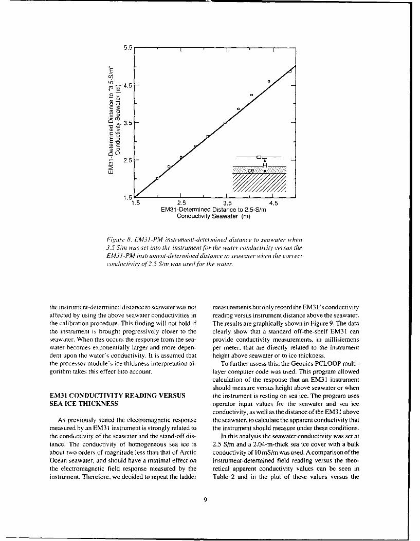
Figure 8. EMSI-PM instrument-deternzined distance to seawater whenl3.5 S/mn was set into the instrumentlfor the water conductivityv versuts theEM31 -PM instrument-deter-mined distance to seawater when the correctc'onductivity of 2.5 S/mi was used fir tire water.

the instrument-determined distance to seawater was not measurements but only record the EM31 I's conductivityaffected by using the above seawater conductivities in reading versus instrument distance above the seawater.the calibration procedure. This finding will not hold if The results are graphically shown in Figure 9. The datathe instrument is brought progressively closer to the clearly show that a standard off-the-shelf EM31 canseawater. When this occurs the response from thae sea- provide conductivity measurements, in rnillisiemcnswater becomes exponentially larger and more depen- per meter. that are directly related to the instrumentdent upon the water's conductivity. It is assumed that height above seawater or to ice thickness.the processor module's ice thickness interpretation al- To further assess this, the Geonics PCLOOP multi-gorithm takes this effect into account. layer computer code was used. This program allowed

calculation of the response that an EM31 instrumentshould measure versus height above seawater or when

EM31 CONDUCTIVITY READING VERSUS the instrument is resting on sea ice. The program usesSEA ICE THICKNESS operator input values for the seawater and sea ice

conductivity, as well as the distance of the EM31 aboveAs previously stated the electromagnetic response the seawater, to calculate the apparent conductivity that

measured by an EM31 instrument is strongly related to the instrument should measure under these conditions.the condLctivity of the seawater and the stand-off dis- In this analysis the seawater conductivity was set attance. The conductivity of homogeneous sea ice is 2.5 S/m and a 2.04-m-thick sea ice cover with a bulkabout two orders of magnitude less than that of Arctic conductivity of I10 mS/m was used. A comparison of theOcean seawater, and should have a minimal effect on instrument-determined field reading versus the theo-the electromagnetic field response measured by the retical apparent conductivity values can be seen ininstrument. Therefore, we decided to repeat the ladder Table 2 and in the plot of these values versus the

~0 9

300 I I I I

E

.5 200

0

U)

S100 _____ __

H

0 1 2 3 4 5 6H, Tape-Measured Distance to Seawater (in)

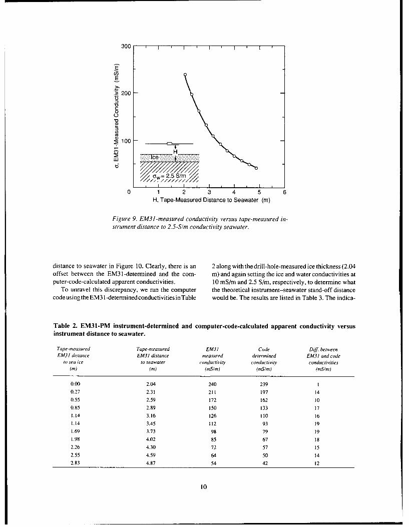
Figure 9. EM3J -measured conductivity versus tape-measured in?-strument distance to 2.5-S/in conductivity seawater.

distance to seawater in Figure 10. Clearly, there is an 2 along with the drill-hole-measured ice thickness (2.04offset between the EM131-deterrnined and the corn- m) and again setting the ice and water conductivities atputer-code-calculated apparent conductivities. 10 mS/rn and 2.5 S/rn, respectively, to determine what

To unravel this discrepancy, we ran the computer the theoretical instrument-seawater stand-off distancecode using the EM3lI-determined conductivities in Table would be. The results are listed in Table 3. The indica-

Table 2. EM31-PM instrument-determined and computer-code-calculated apparent conductivity versusinstrument distance to seawater.

Tape-measured Tape-measured EM31 Code Duff. betweenEM31 distance EM3I distance measured determined EM3J and code

to sea ice to seawater conductivity conductivity conductivities(in (n)(mS/rn) (mS/rn) (ni~m)

0.00 2.04 240 2391

0.27 2.31 211 197 14

0.55 2.59 172 162 10

0.85 2.89 150 133 17

1.14 3.16 126 110 161.14 3.45 112 93 19

1.69 3.73 98 79 19

1.98 4.02 85 67 18

2.26 4.30 72 57 152.55 4.59 64 50 14

2.83 4.87 54 42 12

10

600 1 1 1 1 1 1

Difference4 + Calculated

500 o Measured

E+

(/2400-E +

." 300-

~0-200

oo

+ [

01 2 3 4 5 6H, Tape-Measured Distance to Seawater (m)

Figure 10. EM31 -measured and computer-code determined conduc-tivity versus tape-measured instrument distance to 2.5-S/m-conduc-tivity seawater. Also shown is the difference between the measuredand calculated conductivit, values versus distance.

tion here is that either the EM31 conductivity determi- distances than determined by tape measurement. Innations are wrong or the computer-program calculated addition, subtracting column I from column 4 in Tableinstrument distances to the seawater are in error. From 3 givesthe results incolumn 5, which indicate adecreas-this analysis we found that the computer code consis- ing ice thickness versus increasing instrument heighttently calculated lower instrument-seawater stand-off above the seawater. A plot of these findings is shown in

Table 3. Computer-code-calculated distance to seawater and sea ice thickness using the EM31 field-determined apparent conductivities versus instrument elevation above the seawater.

Tape-measured Tape-measured EM31 Calculated CalculatedEM31 distance EM31 distance measured distance to ice

to sea ice to seawater conductivity seawater thickness(ni (m) (mS/n) () (in)

0 2.04 240 -2.04 -2.04

0.27 2.31 211 2.21 1.940.55 2.59 172 2.50 1.950.85 2.89 150 2.70 1.851.14 3.16 126 2.96 1.821.41 3.45 112 3.15 1.74

1.69 3.73 98 3.35 1.661.89 4.02 85 3.59 1.612.26 4.30 72 3.92 1.66

2.55 4.59 64 4.08 1.532.83 4.87 54 4.39 1.56

11

5 1 1 1 1 1 1 1 1Calculated EM31 Ice Thickness

+- Calculated EM31 Distance to Seawater

4-E

C5

2C

C-,3

0 1 2 3 4 5 6H, Tape-Measured Distance to Seawater (m)

Figure 11. Ice thickness and EM3J instrument stand-off distance

to seawater determined from EM31 measurements versus tape-measured distance to the seawater.

Figure 11. Clearly, there is a problem. The problem two things to happen. First, the coil support booms,turns out to be a relatively simple one, but an extremely extending out each side of the electronic module, butted

important one that must be appreciated by anyone up against the ladder sides. This prevented the elec-

choosing to use an EM31 type instrument for sea ice tronicmodulefromrestingflatonthesteps(seeFig. 12).

thickness determinations. Second, above about the fourth step, the tilt was exac-

Resting the instrument on the ladder steps caused erbated by the narrowing of the sides of the ladder and

i -- 4 mn

Figure 12. Position of EM31 instrument when set on ladder step.

12

by the operator. who stated he had a tendency to tilt the plying the number in column 2 by the sine of the sameunit on the higher steps to make viewing the readout angle.easier. In short, he did not wish to climb any higher on The results of this process are given in columns 5 andthe relatively unstable ladder than was apparently nec- 6 in Table 4. As expected, when the instrument wasessary. This was probably a good idea, considering the resting on the ice surface and was reasonably level, itpoor condition of the stepladder used. gave a conductivity reading (column 4) in excellent

Tilting of the EM31 ca ised the orientation of the agreement with the theoretical value shown in columnvertical co-planar coils to change. Instead of being 3. However, when the instrument was placed on thevertical, as desired and as_,imed in the computer analy- ladder step it was tilted slightly to fit securely in placesis, the coils were tilted sLghtly away from vertical. (Fig. 12). As the instrument was moved onto higher

Fortunately, the computer code allows determina- ladder steps the tilt angle became progressively greater,tion of the theoretical conductivity for both a vertical as shown by column 5 in Table 4.and horizontal co-planar coil position for a given set of Replotting the above corrected data in Figure 1input parameters, such as instrument height, seawater would cause the lines to rotate counterclockwise aboutconductivity (2.5 S/m), ice thickness (2.04 m), ice the 2.04-mi intercept, and the calculated ice thicknessconductivity (10 mS'm), etc. Therefore, the computer curve would became horizontal, as it should be. There-code was used to recalculate the theoretical conduc- fore, good EM31 conductivity measurements shouldtivity for the vertical and horizontal co-planar coil provide for a determination of sea ice thickness eitherpositions above sea.vater at which our EM3 1 field for when the instrument is resting on the ice surface ormeasurements were made. These calculations are given when it is elevated above the ice surface.in Table 4 (columns 2 and 3) along with the EM31 Seawater conductivity will be lower at a coastal sitereading obtained in the field (column 4). Next. tilt angle where a major river, such as the Mackenzie River incorrections were applied to the calculated values in Canada, continues to flow into the ocean during thecolumns 2 and 3 until an angle was found that produced winter. No rivers flow into the Alaskan Beaufort Seaa theoretical conductivity that was in close agreement during the winter.with the field measurement. Foreach instrument height, As previously stated, an EM31 instrument providesthis new value was determined by multiplying the an apparentconductivity reading foragiveninstrumentnumberincolumn3by thecosineofsomecoil tilt angle height above seawater. This reading is unique for a0 and adding this value to the value obtained by multi- specific seawater conductivity and should allow deter-

Table 4. Theoretical versus measured EM31 conductivity as a function of instrument height above 2.04-m-thick sea ice and instrument tilt angle correction required to produce agreement between the theoreticalconductivity for the vertical co-planar coils on the EM31 and the, ctual instrument field reading.

Thteoretical conductivity,

IAM31 dist. E4M31 ,inge New cond.*t, l .d'aH'ter Ilor. (oil Ver. coil readintg correction ver. coil

(I) (11S 1 (oSim) (InShn) (0) finStm)

2.04 292 239 240 0 -2.31 257 197 211 3 2102.59 223 162 172 3 1742.89 192 133 150 5 1493.16 165 110 126 6 1263.45 144 93 112 8 1123.73 123 79 98 9 984.02 108 67 85 to 854.30 94 57 72 10 724.59 82 49 64 11 644.87 72 42 54 I1 55

New theoretical vertical coil conductivity value Ver. coil conductivity x cosO + Hor. coil conductivity x sinO.

13

1000 I '

SeawaterConductivity

) :w= 3.0 S/mE

Z( a,= 2.5 S/ra)cc

> 100

0

t--5

0

H

10 I I I I0 2 4 6

H, Instrument Height Above Seawater (m)

Figure 13. Theoretical EM3J conductivity reading ver-sus instrument height above 2.5- and 3.0-S/m conductiv-ity seawater.

mination of instrument-seawater stand-off distance. seawater having a conductivity of 2.5 S/m. In thisDuring the winter, the seawater under the Arctic Ocean analysis, bulk sea ice conductivities of 10 and 50 mS/mpack ice has a conductivity of 2.5 + 0.05 S/r. An were used. The latter is a high value that may representanalysis was made to show how an EM3 I's conductiv- warm, high-brine-volume sea ice. The former value is aity reading should vary with elevation above seawater reasonable value for arctic winter pack ice. The resultsof 2.5 S/m and an extreme seawater conductivity of 3.0 are plotted in Figure 14. As may be inferred from theseS/r. The results are shown in Figure 13 for vertical co- figures, the error, caused by the two bulk sea iceplanar antenna coils. For heights above about 3 m, there conductivities used, in the distance to the seawater, asis no appreciable difference in instrument reading ver- determined from the instrument conductivity reading,sus seawater conductivity; there is, however, progres- is on the order of 5%. This indicates that the responsesively greater difference as the instrument is brought from the seawater as measured by the instruments willcloser to the water. For example, when the instrument is not be significantly affected by sea ice conductivityI m above seawater having a 2.5-S/m conductivity, the variations.EM31 reading would be about 520 mS/m. However, An EM31 instrument is best used resting on the icethis same reading over 3.0-S/m-conductivity water would surface to avoid potential measurement error associatedoccur when the instrument was about 1. 1 m above the with tilting of the antenna coils. This would be particu-surface. This 10% error for the extreme seawater con- larly desirable on thick ice to maximize the receivedductivities used indicates that the very low offshore signal and to allow thick ice to be measured. If theArctic Ocean conductivity variations will not signifi- instrument must be carried, then some provision shouldcantly affect the ice thickness determinations, be made to show the operator whether or not the

Another series of calculations was made to show instrument is level.how an EM3 I's conductivity reading should vary as the If the instrument conductivity reading is to be used toinstrument is moved from the surface of 1.5- and 2.5-m- infer ice thickness, then a simple table or graph affixedthick sea ice to some elevation above ice floating on to the instrument cover could be used. Such a graph is

14

400 ' I

Ef

300

4) 50 mS/m

-~ 200 o10 m.S/rno Oi =10 rnS/m

2000

0

0 1 2 3 4H, Instrument Height Above Seawater (m)

a. 1.5-m-thick ice.

200

160

E

-C 120

al -50 mS/m

80 O= 10 mS/m00

t5

40-

O. I 13 4 5

H, Instrument Height Above Seawater (m)

b. 2.5-m-thick ice.

Figure 14. Theoretical EM3J conductivity reading versus in-strument height above 2.5-S/r-conductivity seawater coveredwith ice of 10- and 50-mSIm bulk conductivity (csi).

15

1000

- = 70 mS/rn Ic-

70

70E 60E Instrument on Ice0)

C

cr 20 Figure 15. Theoretical EM31 conductivity reading ver-2 sus instrument height above sea water. The ice is resting: _ 100 -on water of 2.5-S/rn conductivity and ice conductivity is"5 - No IceCoe

15 shownz to vary with thickness.-1t-

co

Lu10

Y = Bulk Ice Conductivity

5w = Seawater Conductivity

1 0 1 1 1 I0 2 4 6

H, Instrument Height Above Seawater (m)

shown in Figure 15. This figure shows how the conduc- year sea ice from about 0.7 to about 3.5 m thick, with ativity reading of an EM31 instrument should vary with snow cover, indicated that the EM3 I-PM instrumentsea ice thickness where the underlying seawater has a was providing reasonably good estimates, even if theyconductivity of 2.5 S/m. Another parameter used in weren't accurate enough for our research. The unsatis-construction of the graph is a variable bulk sea ice factory ice thickness measurements were generallyconductivity. These bulk conductivities versus ice obtained in areas of deformed ice where the measuredthickness were obtained from recent work of Kovacs electromagnetic response was adversely affected by( 1991 ). Note that the upper curve applies to an instru- conductive inhomogeneities associatcd with the sub-ment resting on the surface, while the lower curve merged ice block structure.represents the instrument conductivity readings when Further testing of the EM3 1-PM instrument on ano ice layer exists ladder produced ice thickness results that varied with

The sea ice conductivities shown in Figure 15 repre- instrument calibration procedure. This should not oc-sent reasonable upper limit values for the given ice cur. However, other inconsistencies between instru-thickness. Figure 15 is instructive because it indicates ment-determined sea ice thickness and direct tape-that the error associated with ignoring sea ice conduc- measured distances may have resulted from tilting oftivity and assuming that an air layer exists between the the antenna coils. Given this mixed review, anotherinstrument and the seawater will have a minimal eftect field test of the module's measurement performance ison the estimated ice thickness. This is especially true for needed.ice under 3 m thick. Use of the EM3 1-PM instrument in the field proved

frustrating. The instrument frequently quit at tempera-tures below -15'C. We also encountered lithium bat-

GENERAL COMMENTS tery problems. On several occasions one battery, out ofthe set of ten used to run the system, would drop in

Some of the data obtained with the Geonics EM31 voltage. This drop would shut down the unit until theand the Flow Research ice thickness processor module bad battery was found (back in "town") and replaced.showed excessive variation from the drill-hole-mea- This low battery problem caused measurement delayssured ice thickness. However, measuremcnts on first- and may also have caused the cold weather shutdown

16

problem mentioned above. When the instrument was LITERATURE CITEDpicked up in Kent, Washington, new batteries for theinstrument were also obtained. Therefore, the batteries Anderson, W.L. (1979) Computer programs; numeri-should have been good if they were recently manufac- cal integration of related Hankel transforms of order 0tured ones. and I by adaptive digital filtering. Geop-ysics, 44 (7):

There is good reason to believe that a standard EM3 1 1287-1305.instrument can be used to determine sea ice thickness Echert, D.C. (1986) Electromagnetic induction remotefrom about 0.7 to 5 m, to within an accuracy of±10% of sensing of sea ice thickness. Kent, Washington: Flowthe tape-measured value. For this, the instrument's Research Co., Inc., Flow Technical Report No. 388.conductivity readingandatableorgraph could be used; Echert, D.C., G.B. White and A. Becker (1989)such a graph is presented in Figure 15. It may well be Electromagnetic induction sensing of sea ice thicknesspossible to achieve ice thickness determinations within and conductivity. Kent, Washington: Flow Research5% of the actual thickness when on ice of uniform Co., Inc., Flow Technical Report No. 492.thickness. However, further field tests would be needed Geonics, Ltd. (1984) Operating manual for EM3 I-Dto verify this. non-contacting terrain conductivity meter. Mississauga,

In the absence of a theoretical analysis, the EM31 Ontario, Canada.may be calibrated on the sea ice by simply recording the Hoekstra, P., A. Sartorelli and S.B. Shinde (1979) Lowinstrument conductivity reading made at a number of frequency methods for measuring sea ice thickness.heights above the ice/water interface and constructing a International Workshop on the Remote Estimation ofgraph similar to that presented in Figure 4. This calibra- Sea Ice Thickness, Memorial University, St. John's,tion procedure needs only to be done once for arctic sea Nevfoundland, Canada, pp. 313-330.ice sounding, because the conductivity determined by Hoekstra, P. (1980) Theoretical and experimental re-the EM31 is based on the use of the measured quadra- sults of measurements with horizontal magnetic dipoleslure phase response. the zero level of which "is designed over sea water to measure ice thickness and waterto stay at the correct value over the life of the instrument salinity. Geo-Physi-Con Co., Ltd., Calgary, Albertaover wide temperature excursions."* However, a cali- (confidential document).bration check would certainly be appropriate at a loca- Kovacs, A. (1991) Preliminary results of the 1990tion where under-ice water conductivity may not be Alaska remote sounding of sea ice thickness study.known. USA Cold Regions Research and Engineering Labora-

In this report we addressed the use of EMI sounding tory, Internal Report (unpublished).to measure sea ice thickness in the Arctic Ocean. The Kovacs, A. and S.J. Holladay (1989) Development ofpresentation is specific to areas where the under-ice an airborne sea ice thickness measurement system andwater depth is in excess of 6 m. In shallower waters, the field test results. USA Cold Regions Research andresponse from the third layer, the seabed, needs to be Engineering Laboratory, CRREL Report 89-19.addressed. This is beyond our scope here. Kovacs, A., R.M. Morey and G.F.N. Cox (1987a)

It should be kept in mind that EMI sounding does not Modeling the electromagnetic property trends in seagive a pc;7t measurement, but provides an "average" ice, Part I. ColdRegions Science and Technology, 14(3):ice thickness for an area having a diameter of about 207-235.three times the Leight of the instrument above the Kovacs, A., N.D. Valleau and S.J. Holladay (1987b)seawater. Therefore, EMI sounding of multi-year sea Airborne electromagnetic sounding of sea ice thicknessice thickness may result in significant errors where the and sub-ice bathymetry. Cold Regions Science andbottom of the ice has rough, short-period undulations. Technology, 14(3): 289-311.This relief is not uncommon and must be taken under Liu, G. and A. Becker (1990) Two-dimensional map-consideration when multi-year sea ice soundings are ping of sea-ice keels with airborne electromagnetics.made using EMI. Geophysics, 55(2): 239-248.

Sinha, A.K. (1976) A field study for sea ice thickness* Personal communication with J.D, McNeill, Geonics, determination by electromagnetic means. Geological

Ltd.. 1990. Survey of Canada, GSC Paper 76-1 C, pp. 225-228.

17

Form ApprovedREPORT DOCUMENTATION PAGE OMB No. 0704-0188Public reporting burden for this collection of information is estimated to average 1 hour per response, including the time for reviewing irstructions. searching existing data sources, gathenng ardmaintaining the data needed, and completing and reviewing the collection of information. Send comments regarding this burden estimate or any other aspect of this collection of information.including suggestion for reducing this burden, to Washington Headquarters Services, Directorate for Information Operations and Reports, 1215 Jefferson Davis Highway. Suite 1204, Arlington,VA 22202-4302, and to the Office of Management and Budget, Paperwork Reduction Project (0704-0188). Washington, DC 20503.

1 AGENCY USE ONLY (Leave blank) 2. REPORT DATE 3. REPORT TYPE AND DATES COVEREDI June 1991

4. TITLE AND SUBTITLE 5. FUNDING NUMBERS

Evaluation of a Portable Electromagnetic Induction Instrument forMeasuring Sea Ice Thickness C: N6845286MP6003

C: N000140WX4B7146. AUTHORS

Austin Kovacs and Rexford M. Morey

7. PERFORMING ORGANIZATION NAME(S) AND ADDRESS(ES) 8. PERFORMING ORGANIZATIONREPORT NUMBER

U.S. Army Cold Regions Research and Engineering Laboratory CRREL Report 91-1272 Lyme RoadHanover, N.H. 03755-1290

9. SPONSORING/MONITORING AGENCY NAME(S) AND ADDRESS(ES) 10. SPONSORING/MONITORINGAGENCY REPORT NUMBER

Naval Oceanographic and Atmospheric Research Laboratoryand Naval Civil Engineering Laboratory

U.S. Department of Navy

11. SUPPLEMENTARY NOTES

12a. DISTRIBUTION/AVAILABILITY STATEMENT 12b. DISTRIBUTION CODE

Approved for public release; distribution is unlimited.

Available from NTIS, Springfield, Virginia 22161.

13. ABSTRACT (Maximum 200 words)

Field trials using a man-portable Geonics. Ltd., EM31 electromagnetic induction sounding instrument, with a plug-in dataprocessing module, for the remote measurement of sea ice thickness, are discussed. The processing module was made by FlowResearch, Inc., to directly measure sea ice thickness and show the result in a numerical display. The EM3 I-processing modulesystem was capable of estimating ice thickness within 10% of the true value for ice from about 0.7 to 3.5 m thick, the oldestundeformed ice in the study area. However, since seawater under the Arctic pack ice has a relatively uniform conductivity (2.5± 0.05 S/m), a simplified method, which can be used forestimating sea ice thickness using just an EM31 instrument, is discussed.It uses only the EM3 I's conductivity measurement, is easy to put into use and does not rely on theoretically derived look-uptables or phasor diagrams, which may not be accurate for the conditions of the area.

14. SUBJECT TERMS 15. NUMBER OF PAGES

Electromagnetic ice sounding Sea ice 23Remote sea ice measurement Sea ice thickness 16. PRICE CODE

17. SECURITY CLASSIFICATION 18. SECURITY CLASSIFICATION 19. SECURITY CLASSIFICATION 20. LIMITATION OF ABSTRACTOF REPORT OF THIS PAGE OF ABSTRACT

UNCLASSIFIED UNCLASSIFIED UNCLASSIFIED ULNSN 7540-01-280-5500 . ,. ., - . ., . , Standard Form 298 (Rev. 2-89)

Prescribed by ANSI Std Z39-18298-102