Electromagnetic Imaging of Brain Function

Richard M. Leahy, Signal and Image Processing Institute

University of Southern California

Thanks: Felix Darvas, Dimitrios Pantazis,Esen Kucukaltun-Yildirim, John

Mosher, Sylvain Baillet, Tom Nichols

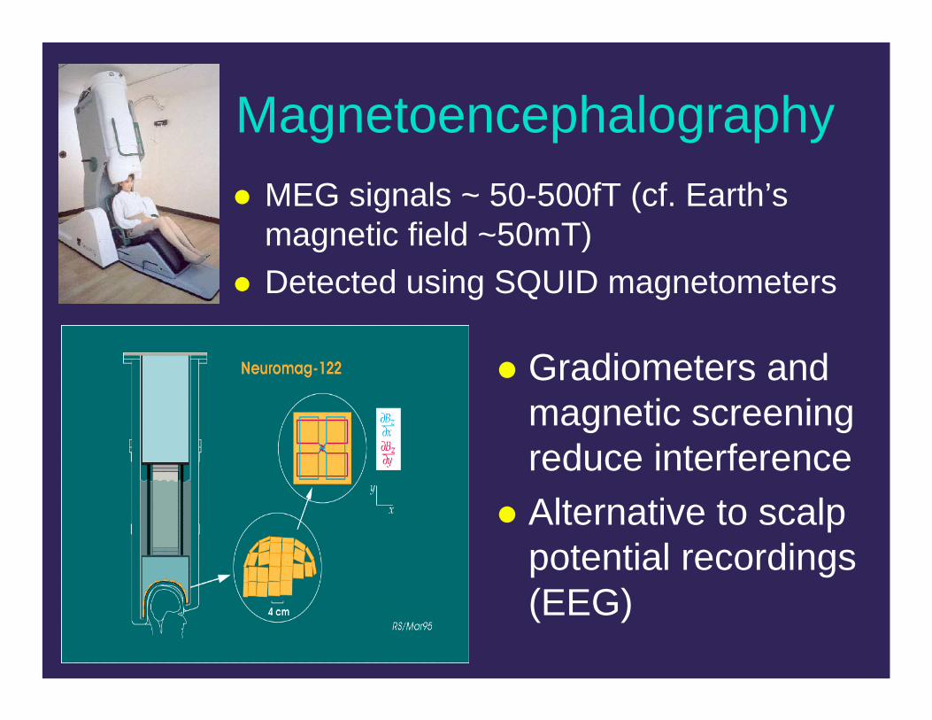
MagnetoencephalographyMEG signals ~ 50-500fT (cf. Earth’s magnetic field ~50mT)Detected using SQUID magnetometers

Gradiometers and magnetic screening reduce interferenceAlternative to scalp potential recordings (EEG)

Neuromagnetic Fields

Magnetic fields are produced by current flow in apical dendrites in cortical pyramidal neurons

Interested in spontaneous and event related fields

Event-locked averaging typically required for adequate SNR in ERPs/ERFsfrom Ritta Salmelin, low temperature lab,

Helsinki university of Technology

Basic Source Model Columnar organization of cortex and spatial functional specialization on cortical surface lead to current dipole modelto represent focal regions of activation.

scalpskull

cortex

activation site

Source Estimation Problem: find one or more current dipoles representing current sources in cortex (with orientation normal to the surface)

Current source

distribution in the brain

Magnetic field

measurement outside the

head

Forward problem

Biot-Savart lawBiot-Savart law

Forward Problem

Forward Models

Use quasistatic EM model to map from current source to measured fieldsInterested in “primary” rather than “volume” currentsSpherical head: closed formReal head shape & cond-uctivity from MR: use BEM or FEM

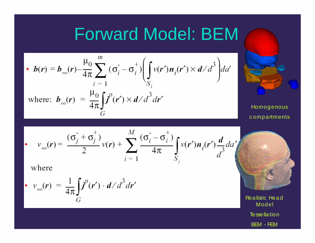
Forward Model: BEM

Homogenous

compartments

Realistic Head Model

Tessellation

BEM - FEM

Tesselated SurfacesSmoothed skull, scalp and brain surfaces for use in BEM forward computationHigh resolution cortical surface for use in cortically constrained imaging

Forward Model: Generic Head

In absence of MRI, use a standard brain/head atlas –warped to subject landmarks – for head modeling (rather than sphere). Use inverse warp to map sources back to stereotactic atlas space for inter-subject studies Warp based on thin-plate spline match of 25 cranial/scalp landmarks:

•X

Z

Y

•

•Fpz

Oz

Mean dipole localization error (n=10 subjects)

vs. true dipole location on

cortex.

Localization using generic head model and TPS warp

Localization using spherical head model and TPS warp

30mm

0mm

50mm

0mm

Current source distribution in

the brain

Magnetic field measurement

outside the head

Forward problem

Biot-Savart lawBiot-Savart law

Forward and Inverse Problems

Source localizationSource localization

Inverse problem

( )

( )Nn KMMM ,1=⎥

⎦

⎤⎢⎣

⎡

⎥⎥⎥

⎦

⎤

⎢⎢⎢

⎣

⎡=

⎥⎥⎥

⎦

⎤

⎢⎢⎢

⎣

⎡

(n)y(n)y

AA

AA

nb

nb

2

1

2M1M

2111

M

1

A11

A21

A12

A22

A13

A23A1M

A2M

y2(n)y1(n)

source2source1Sensor 1

Sensor M

scalp

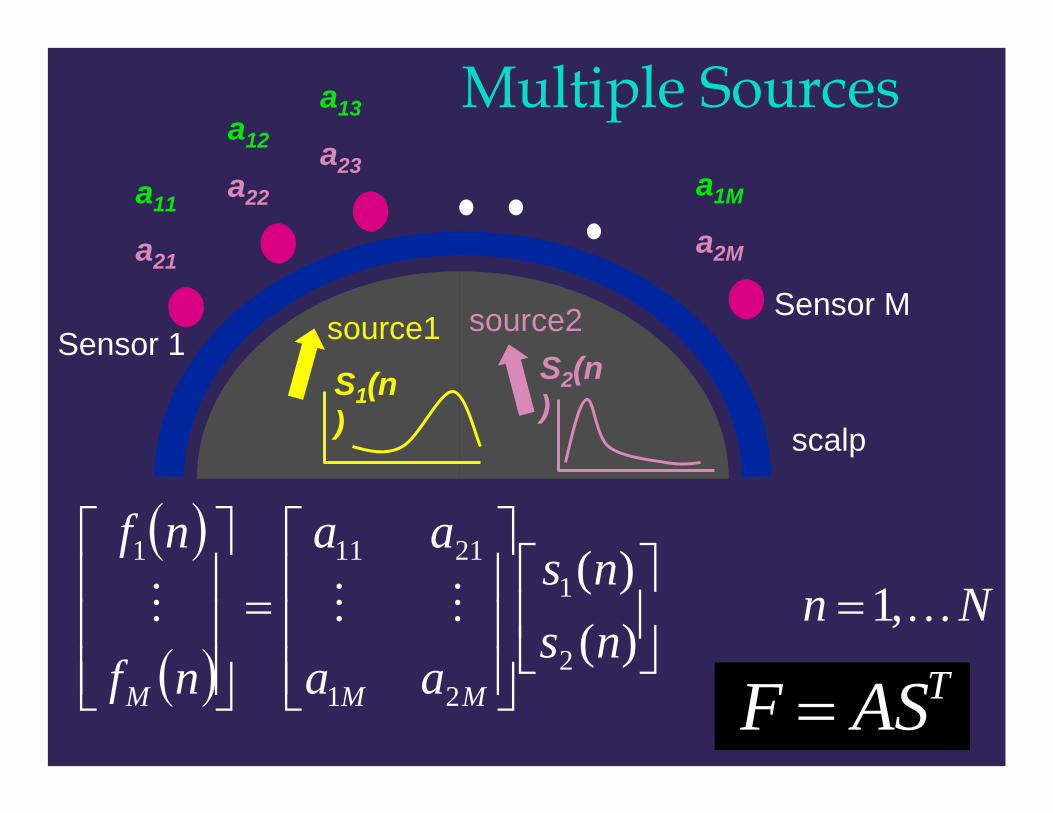
Multiple Sources

General Form of Forward Problem

Magnetic fields are linear function of the dipole amplitudes or momentsMagnetic fields are nonlinear function of the dipole locations and head modelAll inverse methods reduce to (approximately) solving

nAyb +=

Inverse Methods

Competing requirements» Representation of complex spatio-temporal sources» Deal with relatively small number of spatial

measurementsApproaches» Cortically constrained imaging» Parametric source estimation» Scanning beamformers (“virtual depth electrode”)

ImagingPlace current dipole at each element in cortical surface tesselationConstrain dipole orientation using cortical surface normalsSolve resulting set of linear equations for dipole amplitudesEquations highly underdetermined (~300 measurements, 100,000 unknowns?)Use regularization or Bayesian approach

Minimum Norm Imaging

Solve:

Choice of weight function:» : minimum energy solution»

:column-weighted min-norm» where is the

Laplacian operator: LORETA (Pascual-Marqui et al 94)

2

2

2

2min WyAyb λ+−

IW =[ ]Naadiag /1,...,/1 1== normWW

BWW norm= B

Simulation Study122 planar gradiometers (Neuromag-122)

100k cortical triangles

3 distributed sources

Minimum-Norm Solutions

Simulated Estimated

Dynamic Solutions

Improving Image ResolutionIntroduce prior information (fMRI) in weighting function [Dale&Sereno 93, Liu, Belliveau, Dale 98]Non-quadratic penalty function, e.g.

εAybyy pi ≤−= ∑ tosubjectmin

1p

ip

[Jeffs&Leahy 87 (p <1), Matsuura&Okabe 95 (p=1)]Nonlinear Bayesian imaging methods [Bailletet al ‘98, Phillips et al ‘98, Shmidt et al ‘01….]

Sparse Focal Source PriorTriangular Tessellation

+

Pixel of interest

Nine nearest pixels

Complete neighborhood

Q=1, α=0.2,β=0.20Q=2, α=0.2,β=0.06Q=3, α=0.2,β=0.017

Parametric MethodsCurrent dipole fitting» Assume few current dipoles, unknown locations and

moments (Brenner,Williamson,Kaufman 78)» Nonlinear least squares estimation problem with five

parameters per dipole (Wood 82)

» For dynamic data (Scherg Von Cramon 85):

2

2)(min yAb θ−

θ,y

2

2)(min YAB θ−

θ,Y

Limitations of Dipole Modeling

Current dipoles may not adequately represent more distributed activationNon-convex numerical problem

Can be difficult tointepret if sources not in cortex

Use multipolar models

Use subspace scanning methods

Use cortical remapping

a11

a21

a12

a22

a13

a23a1M

a2M

( )

( )Nn

nsns

aa

aa

nf

nf

MMM

KMMM ,1)()(

2

1

21

21111

=⎥⎦

⎤⎢⎣

⎡

⎥⎥⎥

⎦

⎤

⎢⎢⎢

⎣

⎡=

⎥⎥⎥

⎦

⎤

⎢⎢⎢

⎣

⎡

TASF =

S2(n)S1(n

)

source2source1Sensor 1Sensor M

scalp

Multiple Sources

MUSIC Source LocalizationColumn space of F contains linear combinations of “gain vectors” for each source Span of column space can be found from SVD of data:MUSIC:» compute gain vectors for each potential source

location and project onto signal subspace:

[ ] T21 UΣFuuU V==

1≤a

aU T

Cortically Remapped Sources Use patch-growing for cortical remapping

Increasing Source Size/Complexity

ECD 1st Order

Multipole

Multipolar Models

Use of multipolar models in cortical source localization

Virtual Depth ElectrodesAdaptive beamforming or spatial filtering

» Design weights with constraint:

» Control degrees of freedom by minimimzing output power:

( ) ( ) TTT ASxWFxWy 00 ==

( ) ( ) I=xGxW T0

][][min WCWtryyE FTT =

111 ][ −−−= FT

FTT RGGRGW

Solution

- Scan over cortical surface

- weight by noise-only response: “Neural Activity Index”

“The cerebral oscillatory network of parkinsonian resting tremor”

Timmermann et al., Brain, 2002

Performance Analysis And

Validation

Sources of Variability and Error

Background environmental and physiological noiseIntrinsic trial-to-trial variability in brain responseRegistration: MEG vs. anatomyHead modelsData acquisition system model

Quantifying Performance Simulation/theory:» Theoretical: e.g. CR bounds» Monte Carlo simulations» Simulation-based ROC analysis

Phantom studies» Localization accuracy

Real data» bootstrap analysis» Permutation and RF based activation

detection » Cross-modality (MEG vs. fMRI, depth

electrodes….

Dale et al., 2000

Dale et al., Neuron, 2000

MEG vs. Depth electrode data

Phantom Study32 current dipoles in humanskull phantom Ground truth from CT scanMEG data from Neuromag-22Sources fit using R-MUSIC, spherical and realistic BEM forward models

Phantom Localization ErrorsAverage error for 32 dipoles using spherical head model: 4.1mmAverage error for 32 dipoles using BEM head model: 3.4mm

Objective Task-Based Evaluation: ROC analysis

False Positive Fraction= 1.0 − Specificity

True

Pos

itive

Fra

ctio

n=

Sens

itivi

ty

1.0

1.00.0

0.0

An “ROC” curve

Sensitivity: Probability of calling an actually-positive case “Positive”TPF = TP / (TP + FN)Specificity: Probability of calling an actually-negative case “Negative”TNF = TN / (TN + FP)

Objective Task-Based Evaluation: ROC analysis

Standard ROC analysis» Binary decision for the presence of a target; location

known Location-Response ROC (LROC)» Specify the location of a target» Only one target allowed

Free-Response ROC (FROC)» Presentation and detection of multiple targets per image» Suitable for neuroimaging studies; we expect many

simultaneously activated brain areas

Timeseries of two uncorrelated patches randomly positioned on the cortical surface

FROC curves for different regularization parameters (Tiknonov-Regularized Min-Norm reconstruction)

FROC curves for MUSIC, LCMV Beamformer, and Min-Norm reconstruction

Experimental data: Bootstrap of Dipole Localization

Approach: » Epochs can be viewed as a set of independent

realizations of the brain’s response» Sample with replacement from epochs and average to

produce “new” data sets» Apply inverse procedure to each bootstrap data set» Cluster resulting dipoles (GMM)» Estimate statistics (mean and standard deviation) from

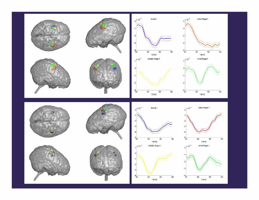
the bootstrap resamplesApplied to somatosensory stimulation data sets for 4 left and right hand digits, 30-60ms post stimulus; 500 trials per digit, 5000 bootstrap resamples

Somatosensory data

Electric stimulation of 4 digits of left and right hand

Locations

Time series

Activation Detection: Control of FWER in Cortical Imaging

Imaging methods result in low resolution reconstruction mapsNoise exhibits highly nonuniform spatial correlationWe need a principled way of identifying true activation versus noise artifactsHow: threshold voxel-wise statistic on the image to control FWER.

Permutation Test

Illustration of the summarizing procedure used to construct empirical distributionsfrom the permuted data:

M permutation samples are produced from the original data . The data are summarized successively in epochs, time and spaceThe empirical distribution of Sj can be used to draw statistical inferences for the original data.

t: Time index

i: Spatial index

j: Permutation index

k: Epoch index

Simulation study

Two sources where simulated. Source 1 (left) and source 2 (right) are shown on the original and smoothed version of a cortical surface. Timecourse of simulated sources and points of source identification at α=0.123. Triangles for both methods, circles for only method 1

Examples of significant activation maps for method 1 and 2 for two time instances. Reconstruction appears spread on the smooth cortical surface, but active sources are in neighboring sulci in the original cortical surface. The lowest achieved FWER for method 2 is α=0.123

Somatosensory study (right thumb)

The data acquisition was done using a CTF Systems Inc. Omega 151 system. The somatosensory stimulation was an electrical square-wave pulse delivered to the right thumb of a healthy right-handed subject.Method 2 appear to be more sensitive. At t = 22 ms it appears tocorrect the current density map, which shows the main activity in the ipsilateral hemisphere.

BrainSuiteBrainStorm

Software:

http://neuroimage.usc.edu