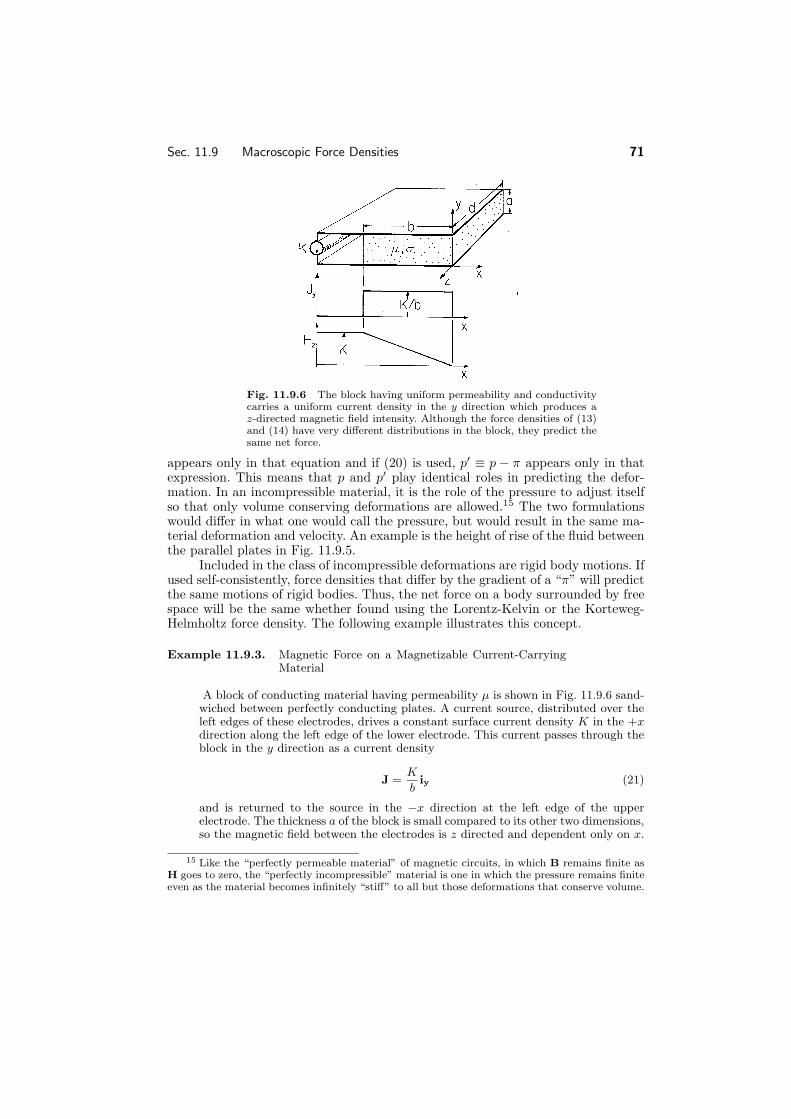
electromagnetic fields and energy - chapter 11: energy - mit
TRANSCRIPT

MIT OpenCourseWare httpocwmitedu
Haus Hermann A and James R Melcher Electromagnetic Fields and Energy Englewood Cliffs NJ Prentice-Hall 1989 ISBN 9780132490207
Please use the following citation format
Haus Hermann A and James R Melcher Electromagnetic Fields and Energy (Massachusetts Institute of Technology MIT OpenCourseWare) httpocwmitedu (accessed [Date]) License Creative Commons Attribution-NonCommercial-Share Alike
Also available from Prentice-Hall Englewood Cliffs NJ 1989 ISBN 9780132490207
Note Please use the actual date you accessed this material in your citation
For more information about citing these materials or our Terms of Use visit httpocwmiteduterms
11
ENERGY POWER FLOW AND FORCES
110 INTRODUCTION
One way to decide whether a system is electroquasistatic or magnetoquasistatic is to consider the relative magnitudes of the electric and magnetic energy storages The subject of this chapter therefore makes a natural transition from the quasistatic laws to the complete set of electrodynamic laws In the order introduced in Chaps 1 and 2 but now including polarization and magnetization1 these are Gaussrsquo law [(621) and (623)]
middot (oE + P) = ρu (1)
Amperersquos law (6211) part times H = Ju + partt
(oE + P) (2)
Faradayrsquos law (927) part times E = minuspartt
microo(H + M) (3)
and the magnetic flux continuity law (922)
middot microo(H + M) = 0 (4)
Circuit theory describes the excitation of a twoshyterminal element in terms of the voltage v applied between the terminals and the current i into and out of the respective terminals The power supplied through the terminal pair is vi One objective in this chapter is to extend the concept of power flow in such a way that power is thought to flow throughout space and is not associated only with
1 For polarized and magnetized media at rest
1
2 Energy Power Flow and Forces Chapter 11
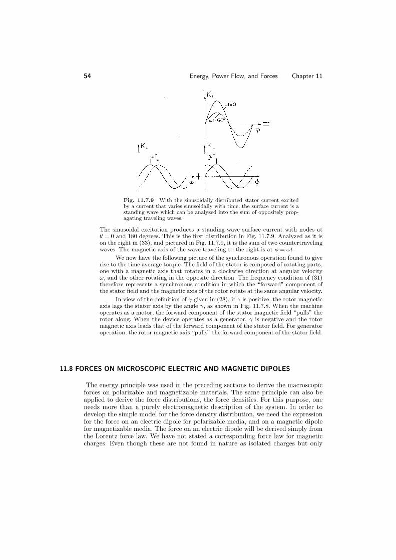
Fig 1101 If the border between two states passes between the plates of a capacitor or between the windings of a transformer is there power flow that should be overseen by the federal government
current flow into and out of terminals The basis for this extension is the laws of electrodynamics (1)ndash(4)
Even if a system can be represented by a circuit the need for the generalization of the circuitshytheoretical power flow concept is apparent if we try to understand how electrical energy is transferred within rather than between circuit elements The limitations of the circuit viewpoint would be crucial to testimony of an expert witness in litigation concerning the authority of the Federal Power Commission2 to regulate power flowing between states If the view is taken that passage of current across a border is a prerequisite for power flow either of the devices shown in Fig 1101 might be installed at the border to ldquolaunderrdquo the power In the first the state line passes through the air gap between capacitor plates while in the second it separates the primary from the secondary in a transformer3 In each case the current never leaves the state where it is generated Yet in the examples shown power generated in one state can surely be consumed in another and a meaningful discussion of how this takes place must be based on a broadened view of power flow
From the circuitshytheoretical viewpoint energy storage and rate of energy dissishypation are assigned to circuit elements as a whole Power flowing through a terminal pair is expressed as the product of a potential difference v between the terminals and the current i in one terminal and out of the other Thus the terminal voltage v and current i do provide a meaningful description of power flow into a surface S that encloses the circuit shown in Fig 1102 The surface S does not pass ldquoinsiderdquo one of the elements
Power Flow in a Circuit For the circuit of Fig 1102 Kirchhoffrsquos laws
2 Now the Federal Energy Regulatory Commission 3 To be practical the capacitor would be constructed with an enormous number of intershy
spersed plates so that in order to keep the state line in the air gap a gerrymandered border would be required Contemplation of the construction of a practical transformer as described in Sec 97 reveals that the state line would be even more difficult to explain in the MQS case
3 Sec 110 Introduction
Fig 1102 Circuit used to review the derivation of energy conservation statement for circuits
combine with the terminal relations for the capacitor inductor and resistor to give
dv i = C + iL + Gv (5)
dt
v = LdiL (6)dt
Motivated by the objective to obtain a statement involving vi we multiply the first of these laws by the terminal voltage v To eliminate the term viL on the right we also multiply the second equation by iL Thus with the addition of the two relations we obtain
vi = vC dv
+ iLLdiL + Gv2 (7)
dt dt
Because L and C are assumed to be constant we can use the relation udu = d(12u2)
to rewrite this expression as
vi = dw
+ Gv2 (8)dt
where 1 1
w = Cv2 + Li2 2 2 L
With its origins solely in the circuit laws (8) can be regarded as giving no more information than inherent in the original laws However it gives insights into the circuit dynamics that are harbingers of what can be expected from the more general statement to be derived in Sec 111 These come from considering some extremes
If the terminals are open (i = 0) and if the resistor is absent (G = 0) w is bull constant Thus the energy w is conserved in this limiting case The solution to the circuit laws must lead to the conclusion that the sum of the electric energy 1Cv2 and the magnetic energy 1Li2 is constant 2 2 L
Again with G = 0 but now with a current supplied to the terminals (8) bull becomes
dw vi = (9)
dt
4 Energy Power Flow and Forces Chapter 11
Because the rightshyhand side is a perfect time derivative the expression can be integrated to give
t
vidt = w(t)minus w(0) (10) 0
Regardless of the details of how the currents and voltage vary with time the time integral of the power vi is solely a function of the initial and final total energies w Thus if w were zero to begin with and vi were positive at some later time t the total energy would be the positive value given by (10) To remove the total energy from the inductor and capacitor vi must be reversed in sign until the integration has reduced w to zero Because the process is reversible we say that the energy w is stored in the capacitor and inductor
If the terminals are again open (i = 0) but the resistor is present (8) shows bull that the stored energy w must decrease with time Because Gv2 is positive this process is not reversible and we therefore say that the energy is dissipated in the resistor
In circuit theory terms (8) is an example of an energy conservation theorem According to this theorem electrical energy is not conserved Rather of the electrishycal energy supplied to the circuit at the rate vi part is stored in the capacitor and inductor and indeed conserved and part is dissipated in the resistor The energy supplied to the resistor is not conserved in electrical form This energy is dissipated in heat and becomes a new kind of energy thermal energy
Just as the circuit laws can be combined to describe the flow of power between the circuit elements so Maxwellrsquos equations are the basis for a fieldshytheoretical view of power flow The reasoning that casts the circuit laws into a power flow statement parallels that used in the next section to obtain the more general fieldshytheoretical law so it is worthwhile to review how the circuit laws are combined to obtain a statement describing power flow
Overview The energy conservation theorem derived in the next two sections will also not be a conservation theorem in the sense that electrical energy is conshyserved Rather in addition to accounting for the storage of energy it will include conversion of energy into other forms as well Indeed one of the main reasons for our interest in power flow is the insight it gives into other subsystems of the physical world [eg the thermodynamic chemical or mechanical subsystems] This will be evident from the topics of subsequent sections
The conservation of energy statement assumes as many special forms as there are different constitutive laws This is one reason for pausing with Sec 111 to summarize the integral and differential forms of the conservation law regardless of the particular application We shall reference these expressions throughout the chapter The derivation of Poyntingrsquos theorem in the first part of Sec 112 is motivated by the form of the general conservation theorem As subsequent sections evolve we shall also make continued reference to this law in its general form
By specializing the materials to Ohmic conductors with linear polarization and magnetization constitutive laws it is possible to make a clear identification of the origins of electrical energy storage and dissipation in media Such systems are considered in Sec 113 where the flow of power from source to ldquosinksrdquo of thermal
5 Sec 111 Conservation Statements
Fig 1111 Integral form of energy conservation theorem applies to system within arbitrary volume V enclosed by surface S
dissipation is illustrated Processes of energy storage and dissipation are developed in greater depth in Secs 114 and 115
Through Sec 115 the assumption is that materials are at rest In Secs 116 and 117 the power input is studied in the presence of motion of materials These sections illustrate how the energy conservation law is used to determine electric and magnetic forces on macroscopic media The discussion in these sections is confined to a determination of total forces Consistent with the field theory point of view is the concept of a distributed force per unit volume a force density Rigorous derivations of macroscopic force densities are based on energy arguments paralleling those of Secs 116 and 117
In Sec 118 we shall look at microscopic models of force density distributions that provide a picture of the origin of these distributions Finally Sec 119 is an introduction to the macroscopic force densities needed to put electromechanical coupling on a continuum basis
111 INTEGRAL AND DIFFERENTIAL CONSERVATION STATEMENTS
The circuit with theoretical conservation theorem (1108) equates the power flowshying into the circuit to the rate of change of the energy stored and the rate of energy dissipation In a field theoretical generalization the energy must be imagined disshytributed through space with an energy density W (joulesm3) and the power is dissipated at a local rate of dissipation per unit volume Pd (wattsm3) The power flows with a density S (wattsm2) a vector so that the power crossing a surface Sa
is given by
Sa S da With these fieldshytheoretical generalizations the power flowing middot
into a volume V enclosed by the surface S must be given by
S da =
d
Wdv +
Pddvminus S
middot dt V V (1)
where the minus sign takes care of the fact that the term on the left is the power flowing into the volume
According to the rightshyhand side of this equation this input power is equal to the rate of increase of the total energy stored plus the power dissipation The total energy is expressed as an integral over the volume of an energy density W Similarly the total power dissipation is the integral over the volume of a power dissipation density Pd
6 Energy Power Flow and Forces Chapter 11
The volume is taken as being fixed so the time derivative can be taken inside the volume integration on the right in (1) With the use of Gaussrsquo theorem the surface integral on the left is then converted to one over the volume and the term transferred to the rightshyhand side
V
middot S + partW
+ Pd
dv = 0 (2)
partt
Because V is arbitrary the integrand must be zero and a differential statement of energy conservation follows
partW middot S + partt
+ Pd = 0 (3)
With an appropriate definition of S W and Pd (1) and (3) could describe the flow storage and dissipation not only of electromagnetic energy but of thermal elastic or fluid mechanical energy as well In the next section we will use Maxwellrsquos equations to determine these variables for an electromagnetic system
112 POYNTINGrsquoS THEOREM
The objective in this section is to derive a statement of energy conservation from Maxwellrsquos equations in the form identified in Sec 111 The conservation theorem includes the effects of both displacement current and of magnetic induction The EQS and MQS limits respectively can be taken by neglecting those terms having their origins in the magnetic induction partmicroo(H + M)partt on the one hand and in the displacement current density part(oE + P)partt on the other
Amperersquos law including the effects of polarization is (1102)
partoE partP times H = Ju + partt
+ partt
(1)
Faradayrsquos law including the effects of magnetization is (1103)
partmicrooH partmicrooM times E = minus partt
minus partt
(2)
These fieldshytheoretical laws play a role analogous to that of the circuit equations in the introductory section What we do next is also analogous For the circuit case we form expressions that are quadratic in the dependent variables Several considerations guide the following manipulations One aim is to derive an expression involving power dissipation or conversion densities and time rates of change of energy storages The power per unit volume imparted to the current density of unpaired charge follows directly from the Lorentz force law (at least in free space) The force on a particle of charge q is
f = q(E + v times microoH) (3)
7 Sec 112 Poyntingrsquos Theorem
The rate of work on the particle is
f v = qv E (4)middot middot
If the particle density is N and only one species of charged particles exists then the rate of work per unit volume is
N f v = qNv E = Ju E (5)middot middot middot
Thus one must anticipate that an energy conservation law that applies to free space must contain the term Ju E In order to obtain this term one should dot multiply middot (1) by E
A second consideration that motivates the form of the energy conservation law is the aim to obtain a perfect divergence of density of power flow Dot multiplication of (1) by E generates ( times H) E This term is made into a perfect divergence if one adds to it minus(times E) H ie if one subtracts (2) dot multiplied by H
middot middot
Indeed (times E) middot Hminus (times H) middot E = middot (Etimes H) (6)
Thus subtracting (2) dot multiplied by H from (1) dot multiplied by E one obtains
times H)part 1
o E
+ E partP minus middot (E =
partt 2 E middot middot
partt
+ part 1
microoH H
partt 2middot
partmicrooM + H + E Ju (7)
middot partt
middot
In writing the first and third terms on the right we have exploited the relation u du = d( 2
1u2) These two terms now take the form of the energy storage term in middot the power theorem (1113) The desire to obtain expressions taking this form is a third consideration contributing to the choice of ways in which (1) and (2) were combined We could have seen at the outset that dotting E with (1) and subtracting (2) after it had been dotted with H would result in terms on the right taking the desired form of ldquoperfectrdquo time derivatives
In the electroquasistatic limit the magnetic induction terms on the right in Faradayrsquos law (2) are neglected It follows from the steps leading to (7) that in the EQS approximation the third and fourth terms on the right of (7) are negligible Similarly in the magnetoquasistatic limit the displacement current the last two terms on the right in Amperersquos law (1) is neglected This implies that for MQS systems the first two terms on the right in (7) are negligible
Systems Composed of Perfect Conductors and Free Space Quasistatic examples in this category are the EQS systems of Chaps 4 and 5 and the MQS systems of Chap 8 where perfect conductors are surrounded by free space Whether quasistatic or electrodynamic in these configurations P = 0 M = 0 and where there is a current density Ju the perfect conductivity insures that E = 0 Thus
8 Energy Power Flow and Forces Chapter 11
the second and last two terms on the right in (7) are zero For perfect conductors surrounded by free space the differential form of the power theorem becomes
partW =
(8)minus middot S
partt
with
S = Etimes H (9)
and
1 1 W = oE E + microoH H
(10)2middot
2middot
where S is the Poynting vector and W is the sum of the electric and magnetic energy densities The electric and magnetic fields are confined to the free space regions Thus power flow and energy storage pictured in terms of these variables occur entirely in the free space regions
Limiting cases governed by the EQS and MQS laws respectively are disshytinguished by having predominantly electric and magnetic energy densities The following simple examples illustrate the application of the power theorem to two simple quasistatic situations Applications of the theorem to electrodynamic sysshytems will be taken up in Chap 12
Example 1121 Plane Parallel Capacitor
The plane parallel capacitor of Fig 1121 is familiar from Example 331 The circular electrodes are perfectly conducting while the region between the electrodes is free space The system is driven by a voltage source distributed around the edges of the electrodes Between the electrodes the electric field is simply the voltage divided by the plate spacing (336)
v E = iz (11)
d
while the magnetic field that follows from the integral form of Amperersquos law is (3310)
r H = o
d v iφ (12)
2 dt d
Consider the application of the integral version of (8) to the surface S enclosing the region between the electrodes in Fig 1121 First we determine the power flowing into the volume through this surface by evaluating the leftshyhand side of (8) The density of power flow follows from (11) and (12)
r o dv S = Etimes H = minus
2 d2 v ir (13)
dt
9 Sec 112 Poyntingrsquos Theorem
Fig 1121 Plane parallel circular electrodes are driven by a disshytributed voltage source Poynting flux through surface denoted by dashed lines accounts for rate of change of electric energy stored in the enclosed volume
The top and bottom surfaces have normals perpendicular to this vector so the only contribution comes from the surface at r = b Because S is constant on that surface the integration amounts to a multiplication
Etimes H da = (2πbd)
b o v
dv =
d 1 Cv2
(14)minus
S
middot 2 d2 dt dt 2
where πb2o
C equiv d
Here the expression has been written as the rate of change of the energy stored in the capacitor With E again given by (11) we doubleshycheck the expression for the time rate of change of energy storage
d
1 d
1 2) v 2
d 1 2
oE Edv = o(dπb = Cv (15)
dt 2 middot
dt 2 d dt 2V
From the field viewpoint power flows into the volume through the surface at r = b and is stored in the form of electrical energy in the volume between the plates In the quasistatic approximation used to evaluate the electric field the magnetic energy storage is neglected at the outset because it is small compared to the electric energy storage As a check on the implications of this approximation consider the total magnetic energy storage From (12)
b 1 1
1 o
dv 2 2 microoH Hdv = microo d r 2πrdr
2 middot
2 2 d dtV 0 (16)
microoob2
C dv 2
= 16 dt
Comparison of this expression with the electric energy storage found in (15) shows that the EQS approximation is valid provided that
microoob2 dv 2 2 (17) v
8 dt
For a sinusoidal excitation of frequency ω this gives
radicbω
8 c 1
2 (18)
10 Energy Power Flow and Forces Chapter 11
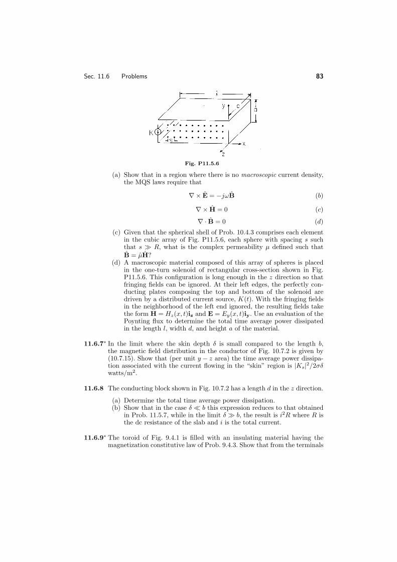
Fig 1122 Oneshyturn solenoid surrounding volume enclosed by surface S denoted by dashed lines Poynting flux through this surface accounts for the rate of change of magnetic energy stored in the enclosed volume
where c is the free space velocity of light (3116) The result is familiar from Example 331 The requirement that the propagation time bc of an electromagnetic wave be short compared to a period 1ω is equivalent to the requirement that the magnetic energy storage be negligible compared to the electric energy storage
A second example offers the opportunity to apply the integral version of (8) to a simple MQS system
Example 1122 Long Solenoidal Inductor
The perfectly conducting oneshyturn solenoid of Fig 1122 is familiar from Example 1012 In terms of the terminal current i = Kd the magnetic field intensity inside is (10114)
i H = iz (19)
d
while the electric field is the sum of the particular and conservative homogeneous parts [(10115) for the particular part and Eh for the conservative part]
microo dHzE = riφ + Eh (20)minus
2 dt
Consider how the power flow through the surface S of the volume enclosed by the coil is accounted for by the time rate of change of the energy stored The Poynting flux implied by (19) and (20) is
microoa d 1 i
S = Etimes H = minus
2d2 dt 2 i2
+
dEφh ir (21)
This Poynting vector has no component normal to the top and bottom surfaces of the volume On the surface at r = a the first term in brackets is constant so the integration on S amounts to a multiplication by the area Because Eh is irrotational the integral of Eh ds = Eφhrdφ around a contour at r = a must be zero For this middot reason there is no net contribution of Eh to the surface integral
Etimes H da = 2πad
microoa d 1 i2
=
d 1 Li2
(22)minus
S
middot 2d2 dt 2 dt 2
Sec 113 Linear Media 11
where microoπa2
L equiv d
Here the result shows that the power flow is accounted for by the rate of change of the stored magnetic energy Evaluation of the right hand side of (8) ignoring the electric energy storage indeed gives the same result
d
1 d
2 1 microo
i 2
d 1 2
microoH Hdv = πa d = Li (23)
dt 2 middot
dt 2 d dt 2V
The validity of the quasistatic approximation is examined by comparing the magshynetic energy storage to the neglected electric energy storage Because we are only interested in an order of magnitude comparison and we know that the homogeshyneous solution is proportional to the particular solution (10121) the latter can be approximated by the first term in (20)
1 oE Edv
1 o
micro2 o
di 2d
a
r 22πrdr
2 middot
2 4d2 dtV 0 (24)
microooa 2 L di 2
= 16 dt
We conclude that the MQS approximation is valid provided that the angular freshyquency ω is small compared to the time required for an electromagnetic wave to propagate the radius a of the solenoid and that this is equivalent to having an elecshytric energy storage that is negligible compared to the magnetic energy storage
microooa 2 di 2 i2 ωa 2 1 (25)
8 dt rarr radic
8c
A note of caution is in order If the gap between the ldquosheetrdquo terminals is made very small the electric energy storage of the homogeneous part of the E field can become large If it becomes comparable to the magnetic energy storage the structure approaches the condition of resonance of the circuit consisting of the gap capacitance and solenoid inductance In this limit the MQS approximation breaks down In practice the electric energy stored in the gap would be dominated by that in the connecting plates and the resonance could be described as the coupling of MQS and EQS systems as in Example 341
In the following sections we use (7) to study the storage and dissipation of energy in macroscopic media
113 OHMIC CONDUCTORS WITH LINEAR POLARIZATION AND MAGNETIZATION
Consider a stationary material described by the constitutive laws
P = oχeE
microoM = microoχmH (1)
12 Energy Power Flow and Forces Chapter 11
Ju = σE
where the susceptibilities χe and χm and hence the permittivity and permeability and micro as well as the conductivity σ are all independent of time Expressed in terms of these constitutive laws for P and M the polarization and magnetization terms in (1127) become
E partP
= part 1
oχeE Emiddot
partt partt 2 middot
H partmicrooM
= part 1
microoχmH H
(2)middot partt partt 2
middot
Because these terms now appear in (1127) as perfect time derivatives it is clear that in a material having ldquolinearrdquo constitutive laws energy is stored in the polarshyization and magnetization processes
With the substitution of these terms into (1127) and Ohmrsquos law for Ju a conservation law is obtained in the form discussed in Sec 111 For an electrically and magnetically linear material that obeys Ohmrsquos law the integral and differential conservation laws are (1111) and (1113) respectively with
S = Etimes H (3a)
1 1 W = E E + microH H
2middot
2middot
(3b)
Pd = σE E (3c)middot
The power flux density S and the energy density W appear as in the free space conshyservation theorem of Sec 112 The energy storage in the polarization and magnetishyzation is included by simply replacing the free space permittivity and permeability by and micro respectively
The term Pd is always positive and seems to represent a rate of power loss from the electromagnetic system That Pd indeed represents power converted to thermal form is motivated by considering the origins of the Ohmic conduction law In terms of the bipolar conduction model introduced in Sec 71 positive and negative carriers respectively experience the forces f+ and f These forces areminusbalanced by collisions with the surrounding particles and hence the work done by the field in forcing the migration of the particles is converted into thermal energy If the velocity of the families of particles are respectively v+ and v and the minusnumber densities N+ and N respectively then the rate of work performed on the carriers (per unit volume) is
minus
Pd = N+f+ v+ + N f v (4)middot minus minus middot minus
Sec 113 Linear Media 13
In recognition of the balance between collision forces and electrical forces the forces of (4) are replaced by |q+|E and minus|qminus|E respectively
Pd = N+ q+ E v+ minus N q E v (5)| | middot minus| minus| middot minus
If in turn the velocities are written as the products of the respective mobilities and the macroscopic electric field (713) it follows that
Pd = (N+ q+ micro+ + N q micro )E E = σE E (6)| | minus| minus| minus middot middot
where the definition of the conductivity σ (717) has been used The power dissipation density Pd = σE E (wattsm3) represents a rate of middot
energy loss from the electromagnetic system to the thermal system
Example 1131 The Poynting Vector of a Stationary Current Distribution
In Example 752 we studied the electric fields in and around a circular cylindrical conductor fed by a battery in parallel with a diskshyshaped conductor Here we detershymine the Poynting vector field and explore its spatial relationship to the dissipation density
First within the circular cylindrical conductor [region (b) in Fig 1131] the electric field was found to be uniform (757)
b v E = iz (7)
L
while in the surrounding free space region it was [from (7511)]
v Ea = minus
L ln(ab)
z
r ir + ln(ra)iz
(8)
and in the diskshyshaped conductor [from (759)]
v 1 Ec = ir (9)
ln(ab) r
By symmetry the magnetic field intensity is φ directed The φ component of H is most easily evaluated from the integral form of Amperersquos law The current density in the circular conductor follows from (7) as Jo = σvL Then
2 b Jor 2πrHφ = Joπr Hφ = r lt b (10)rarr
2
Job2
2πrHφ = Joπb2 rarr Hφa =
2r b lt r lt a (11)
The magnetic field distribution in the disk conductor is also deduced from Amp` erersquos law In this region it is easiest to evaluate the r component of Amp` erersquos differential law with the current density Jc = σEc with Ec given by (9) Integrashytion of this partial differential equation on z then gives a linear function of z plus
14 Energy Power Flow and Forces Chapter 11
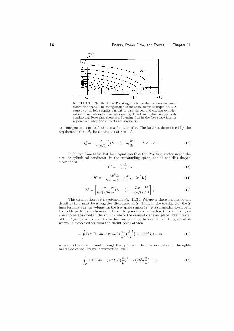
Fig 1131 Distribution of Poynting flux in coaxial resistors and assoshyciated free space The configuration is the same as for Example 752 A source to the left supplies current to diskshyshaped and circular cylindrishycal resistive materials The outer and rightshyend conductors are perfectly conducting Note that there is a Poynting flux in the free space interior region even when the currents are stationary
an ldquointegration constantrdquo that is a function of r The latter is determined by the requirement that Hφ be continuous at z = minusL
σ v b2
Hφc = minus
ln(ab) r (L + z) + Jo
2r b lt r lt a (12)
It follows from these last four equations that the Poynting vector inside the circular cylindrical conductor in the surrounding space and in the diskshyshaped electrode is
Sb = minus L
v J
2 o rir (13)
Sa vb2Jo z r
= minus ln(ab)2rL r
iz minus ln a ir
(14)
Sc =
minusσ v 2
(L + z) + Jov b2
iz (15)
ln2(ab) r2 ln(ab) 2r2
This distribution of S is sketched in Fig 1131 Wherever there is a dissipation density there must be a negative divergence of S Thus in the conductors the S lines terminate in the volume In the free space region (a) S is solenoidal Even with the fields perfectly stationary in time the power is seen to flow through the open space to be absorbed in the volume where the dissipation takes place The integral of the Poynting vector over the surface surrounding the inner conductor gives what we would expect either from the circuit point of view
2 minus Etimes H middot da = (2πbL)
L
v J2 ob
= v(πb Jo) = vi (16)
where i is the total current through the cylinder or from an evaluation of the rightshyhand side of the integral conservation law
2 2 v
σE Edv = (πb L)σ v 2
= vπb σ
= vi (17)middot
L LV
Sec 113 Linear Media 15
An Alternative Conservation Theorem for Electroquasistatic Systems In describing electroquasistatic systems it is inconvenient to require that the magnetic field intensity be evaluated We consider now an alternative conservation theorem that is specialized to EQS systems We will find an alternative expression for S that does not involve H In the process of finding an alternative distribution of S we illustrate the danger of ascribing meaning to S evaluated at a point rather than integrated over a closed surface
In the EQS approximation E is irrotational Thus
E = (18)minusΦ
and the power input term on the left in the integral conservation law (1111) can be expressed as
minus S
Etimes H middot da = S
Φtimes H middot da (19)
Next the vector identity
times (ΦH) = Φtimes H + Φtimes H (20)
is used to write the rightshyhand side of (19) as
minus
S
Etimes H middot da = S
times (ΦH) middot da minus S
Φtimes H middot da (21)
The first integral on the right is zero because the curl of a vector is divergence free and a field with no divergence has zero flux through a closed surface Amperersquos law can be used to eliminate curl H from the second
Etimes H da =
Φ
J +
partD da (22)minus
S
middot minus S partt
middot
In this way we have determined an alternative expression for S valid only in the electroquasistatic approximation
S = ΦJ +
partD
partt (23)
The density of power flow expressed by (23) as the product of a potential and total current density consisting of the sum of the conduction and displacement current densities has a form similar to that used in circuit theory
The power flux density of (23) is convenient in describing EQS systems where the effects of magnetic induction are not significant To be consistent with the EQS approximation the conservation law must be used with the magnetic energy density neglected
Example 1132 Alternative EQS Power Flux Density for Stationary Current Distribution
16 Energy Power Flow and Forces Chapter 11
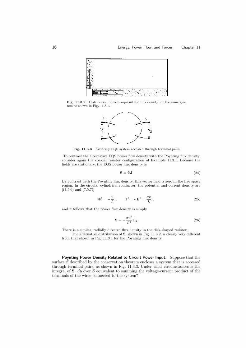
Fig 1132 Distribution of electroquasistatic flux density for the same sysshytem as shown in Fig 1131
Fig 1133 Arbitrary EQS system accessed through terminal pairs
To contrast the alternative EQS power flow density with the Poynting flux density consider again the coaxial resistor configuration of Example 1131 Because the fields are stationary the EQS power flux density is
S = ΦJ (24)
By contrast with the Poynting flux density this vector field is zero in the free space region In the circular cylindrical conductor the potential and current density are [(756) and (757)]
b v b b σv Φ = minus
Lz J = σE =
L iz (25)
and it follows that the power flux density is simply
σv2
S = minus L2
ziz (26)
There is a similar radially directed flux density in the diskshyshaped resistor The alternative distribution of S shown in Fig 1132 is clearly very different
from that shown in Fig 1131 for the Poynting flux density
Poynting Power Density Related to Circuit Power Input Suppose that the surface S described by the conservation theorem encloses a system that is accessed through terminal pairs as shown in Fig 1133 Under what circumstances is the integral of S da over S equivalent to summing the voltageshycurrent product of the middot terminals of the wires connected to the system
Sec 114 Energy Storage 17
Two attributes of the fields on the surface S enclosing the system are required First the contribution of the magnetic induction to E must be negligible on S If this is so then regardless of what is inside S (for example both EQS and MQS systems) on the surface S the electric field can be taken as irrotational It follows that in taking the integral over a closed surface of the Poynting power density we can just as well use (23)
Etimes H da =
Φ
J +
partD da (27)minus
S
middot minus S partt
middot
By contrast with the EQS systems treated in deriving this expression it now holds only on the surface S not necessarily on surfaces inside the volume enclosed by S
Second on the surface S the contribution of the displacement current must be negligible This is equivalent to requiring that S is chosen parallel to the disshyplacement flux density In this case the total power into the system reduces to
minus S
Etimes H middot da = minus S
ΦJ middot da (28)
The integrand has value only where the surface S intersects a wire If taken as perfectly conducting (but nevertheless in a region where partBpartt is zero and hence E is irrotational) the wires have potentials that are uniform over their crossshysections Thus in (28) Φ is equal to the voltage of the terminal In integrating the current density over the crossshysection of the wire note that da is directed out of the surface while a positive terminal current is directed into the surface Thus
n Etimes H da =
viii (29)minus
S
middot i=1
and the input power expressed by (28) is equivalent to what would be expected from circuit theory
Poynting Flux and Electromagnetic Radiation Power cannot be supplied to or lost by a quasistatic system of finite extent through a surface at infinity Such a power supply or loss requires radiation and electromagnetic waves are neshyglected when either the magnetic induction or the displacement current density are neglected To prove this statement consider an EQS system of finite net charge Its electric field intensity decays like 1r2 at infinity where r is the distance to a farshyoff point from some origin chosen within the system At a great distance the currents appear equivalent to current loop sources Hence the magnetic field intenshysity has the 1r3 decay typical of a magnetic dipole It follows that the Poynting vector decays at least as fast as 1r5 so that the flux of Etimes H integrated over the ldquosphererdquo at infinity of area 4πr2 gives zero contribution Because it is only that part of Etimes H resulting from electromagnetic radiation that contributes at infinity Poyntingrsquos theorem is shown in Sec 125 to be a powerful tool for dealing with antennae
18 Energy Power Flow and Forces Chapter 11
Fig 1141 Singleshyvalued constitutive laws showing energy density associshyated with variables at the endpoints of the curves (a) electric energy density and (b) magnetic energy density
114 ENERGY STORAGE
In the conservation theorem (1127) we have identified the terms E partPpartt and middot H partmicrooMpartt as the rate of energy supplied per unit volume to the polarization and middot magnetization of the material For a linear isotropic material we found that these terms can be written as derivatives of energy density functions In this section we seek a more general description of energy storage First nonlinear materials are considered from the field viewpoint Then for those systems that can be described in terms of electrical terminal pairs energy storage is formulated in terms of terminal variables We will find the results of this section directly applicable to finding electric and magnetic forces in Secs 116 and 117
Energy Densities Consider a material in which E and D equiv (oE + P) are collinear With E and D representing the magnitudes of these vectors this material is presumed to be described by a constitutive law in which E is a singleshyvalued function of D such as that sketched in Fig 1141a In the case of a linear constitutive law the curve is a straight line with a slope equal to the permittivity
Consider a material in which E and P are collinear (isotropic material) Then of course E and D equiv oE+P are collinear as well One may graph the magnitude of D versus E and obtain a complete characterization of the material Now the power per unit volume imparted to the polarization is E partPpartt If one adds to it the rate middot of energy supply to the field per unit volume (the free space part) E partoEpartt one middot obtains for the power per unit volume
part partD partD E (oE + P) = E = E middot
partt middot
partt partt (1)
The power supplied to the unit volume can now be written as the time derivative of a function of D We(D) Indeed if we define the area above the graph in Fig 1141 as We then
partWe partWe partD partD = = E
partt partD partt partt (2)
Sec 114 Energy Storage 19
Thus E(partDpartt) is the derivative of the function We(D) This function is the energy stored per unit volume because the energy supplied per unit volume expressed by the integral
t partD
D
dtE = EδD = We(D) (3) minusinfin partt 0
is a function of the final value D of the displacement flux and we assumed that the fields E and D were zero at t = minusinfin Here δD represents the differential of D usually denoted by dD We will use δ rather than d to avoid confusion between difshyferentials used in carrying out volume surface and line integrals and the differential used here which implies an integration in a ldquostate spacerdquo having the ldquodimensionrdquo D
Similar arguments show that if B equiv microo(H + M) and H are collinear and if H is a singleshyvalued function of B then
partB partWmH = middot partt partt (4)
where
B
Wm = Wm(B) = HδB 0 (5)
With (1) and (4) replacing the first four terms on the right in the energy theorem of (1127) it is clear that the energy density W = We + Wm The electric and magnetic energy densities have the geometric interpretations as areas on the graphs representing the constitutive laws in Fig 1141
Energy Storage in Terms of Terminal Variables It was shown in Sec 113 that the power input to a system could be represented by the sum of the vi products for each of the terminal pairs (11329) provided certain conditions were met in the neighborhoods of the terminals The description of energy storage in a lossshyfree system in terms of terminal variables will be found useful in determining electric and magnetic forces With the assumption that all of the power input to a system is accounted for by a time rate of change of the energy stored the energy conservation statement for a system becomes
n viii =
dw (6)
dt i=1
where w = Wdv
V
and the integral is carried over the volume of the system If the system is electroquashysistatic conservation of charge requires that the terminal current be the time rate of change of the charge on the electrode to which the positive terminal is attached
20 Energy Power Flow and Forces Chapter 11
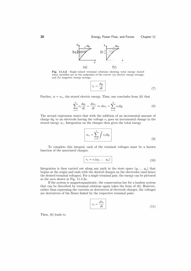
Fig 1142 Singleshyvalued terminal relations showing total energy stored when variables are at the endpoints of the curves (a) electric energy storage and (b) magnetic energy storage
dqiii =
dt (7)
Further w = we the stored electric energy Thus one concludes from (6) that
n n vi
dqi = dwe
dwe =
vidqi (8)dt dt
rArri=1 i=1
The second expression states that with the addition of an incremental amount of charge dqi to an electrode having the voltage vi goes an incremental change in the stored energy we Integration on the charges then gives the total energy
n
we =
vidqi
i=1 (9)
To complete this integral each of the terminal voltages must be a known function of the associated charges
vi = vi(q1 qn) (10)
Integration is then carried out along any path in the state space (q1 qn) that begins at the origin and ends with the desired charges on the electrodes (and hence the desired terminal voltages) For a single terminal pair the energy can be pictured as the area shown in Fig 1142a
If the system is magnetoquasistatic the conservation law for a lossless system that can be described by terminal relations again takes the form of (6) However rather than expressing the currents as derivatives of electrode charges the voltages are derivatives of the fluxes linked by the respective terminal pairs
dλi vi =
dt (11)
Then (6) leads to
Sec 114 Energy Storage 21
Fig 1143 Capacitor partially filled by free space and by dielectric having permittivity
n
wm = iidλi
i=1 (12)
To complete this integral we require the terminal currents as functions of the terminal flux linkages
ii = ii(λi λn) (13)
For a single terminal pair system wm is portrayed in Fig 1142b The most general way to compute the total energy stored in a system is to
integrate the energy densities given by (3) and (5) over the volumes of the respective systems If systems can be described in terms of terminal relations and are loss free (9) and (12) must lead to the same answers Note that (D E) and (q v) are the field and circuit variables in the EQS systems while (B H) and (λ i) have corresponding roles in MQS systems
Example 1141 An Electrically Linear System
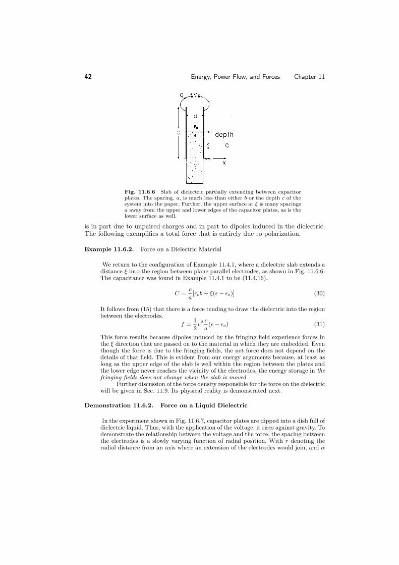
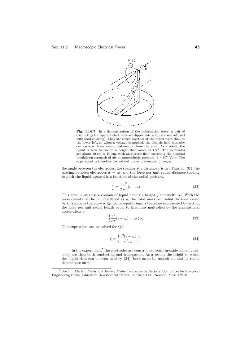
A dielectric slab of permittivity partially fills the region between plane parallel perfectly conducting electrodes as shown in Fig 1143 With the fringing field ignored we find the total energy stored by two methods First the energy density is integrated over the volume Then the terminal relation is used to evaluate the total energy
An exact solution for the electric field well between the electrodes is simply E = ix(va) Note that this field satisfies the boundary conditions at the interface between the dielectric slab and the free space region above and at the electrodes We assume that a b and therefore neglect the fringing fields
The energy density in the linear dielectric where D = E follows from evalshyuation of (3)
D 1 D2
1 2We = EδD = = E (14)
2 20
22 Energy Power Flow and Forces Chapter 11
v E =
a
In the free space region the same result applies with orarrIntegration of these energy densities over the regions in which they apply
amounts to a multiplication by the respective volumes Thus the total energy is
we =
WedV =
1 v 2
(ξca) + 1 o
v 2 [(bminus ξ)ca] (15)
2 a 2 aV
Note that this expression takes the form
1 2 we = Cv (16)2
where c C equiv
a [ob + ξ(minus o)]
In terms of the terminal variables where q = Cv the total energy follows from an evaluation of (9)
2
q 1 q 1 we = vdq = dq = = Cv2 (17)
C 2 C 2
Once the integration has been carried out the last expression is written by again using the relation q = Cv Note that the volume integration of the energy density and the integration in terms of the terminal variables give the same result
The next example considers an MQS system with two terminal pairs and thus illustrates the integration called for in evaluating the energy from the terminal relations Also the energy stored in coupled inductors is often of practical interest
Example 1142 Coupled Coils Transformers
An example of a two terminal pair lossless MQS system is a pair of coupled coils having the terminal relations
λ1
=
L11 L12
i1
(18)
λ2 L21 L22 i2
In this case (12) becomes
dwm = i1dλ1 + i2dλ2 (19)
To evaluate this expression we need to substitute for the currents written in terms of the flux linkages This requires the inversion of (18) For linear systems this is easily done but not for nonlinear systems To avoid inversion we rewrite the rightshyhand side of (19) which becomes
dwm = d(i1λ1 + i2λ2)minus λ1di1 minus λ2di2 (20)
and regroup terms
Sec 114 Energy Storage 23
Fig 1144 Integration path in state space consisting of terminal currents
dwm = λ1di1 + λ2di2 (21)
where the coenergy is defined as
w = m (i1λ1 + i2λ2)minus wm (22)
Equation (21) can be integrated when the flux linkages are expressed in terms of the currents and that is the form in which the terminal relations are given by (18) Once the coenergy w has been found wm follows from (22) m
The integration of (19) is a line integral in a state space (i1 i2) If energy is conserved we must be able to carry out this integration along any path that begins with the currents turned off and ends with the currents at the desired values In the path represented by Fig 1144 the current i1 is turned up first while holding the current i2 to zero Then with i1 held fixed at its final value the current i2 is raised from zero to its final value For this path the integration of (22) becomes
i1 i2
w = λ1(i1 0)di λ2(i1 i2
)di (23) 0 0
m 1 + 2
Substitution for the flux linkages from (18) and evaluation of the integrals then gives
wm =
1 L11i1
2 + L12i1i2 +1 L22i2
2 (24)2 2
If the integration is carried out along a path where the roles of i1 and i2 are reshyversed the expression obtained is (24) with L12 L21 To make the energy stored rarrindependent of path the mutual inductances must be equal
L12 = L21 (25)
This relation which we found to hold for the transformer of Example 974 is reshyquired if energy is to be conserved The energy is now evaluated by substituting this expression and the flux linkages expressed using (18) into (22) solved for wm It follows that
w = wm (26)m
Evaluation of the energy stored in a unityshycoupled transformer where the inductances take the form of (9720) gives
Amicro 1 2 2 1 2 2 wm = N1 i1 + N1N2i1i2 + N2 i2
(27)l 2 2
24 Energy Power Flow and Forces Chapter 11
Operating under ldquoidealrdquo conditions [in the sense that i2i1 = minusN1N2 (9713)] the transformer does not store energy wm = 0 Thus according to the power theorem in the form of (6) under ideal operating conditions the power input at one terminal pair instantaneously appears as a power output at the second terminal pair
Examples have so far involved linear polarization and magnetization constitushytive laws In the following the EQS energy storage in a material having a nonlinear polarization constitutive law is determined
Example 1143 Energy Storage in Electrically Nonlinear Material
To represent the tendency of the polarization to saturate as the electric field is raised a constitutive law might take the form
α1
D = + o E (28)radic
1 + α2E2
Here α1 and α2 are parameters descriptive of the specific material and D is collinear with E This constitutive law is portrayed graphically in Fig 1145
Because D is given as a function of E that is not easily solved for E as a funcshytion of D the computation of the electric energy density using (3) is inconvenient However we can observe that
δWe = EδD = δ(ED)minus DδE (29)
and then regroup terms so that the expression becomes
δWe = DδE (30)
where
We = ED minus We (31)
Integration now leads to the coenergy density We but the energy density We can
then be found using (31) and the constitutive law Specifically evaluation of (30) using (28) gives the coenergy density
We =
DδE =
α1
1 + α2E2 minus 1
+1 oE
2 (32)α2 2
It follows from (31) that the energy density is
We = ED minus We =
α1
radic1 + α2E2 minus 1
+
1 oE
2 (33)α2
radic1 + α2E2 2
A graphical representation of the energy and coenergy functions is given in Fig 1145 The area ldquounder the curverdquo with D as the integration variable is We (3) and the area under the curve with E as the integration variable is We
(31)
Sec 115 Electromagnetic Dissipation 25
Fig 1145 Singleshyvalued nonlinear constitutive law Areas representshying energy density W and coenergy density W are not equal in this case
115 ELECTROMAGNETIC DISSIPATION
The heat generated by electromagnetic fields is often the controlling feature of an engineering design Semiconductors inevitably produce heat and the distribution and magnitude of the heat source is an important consideration whether the apshyplication is to computers or power conversion Often the generation of heat poses a fundamental limitation on the performance of equipment Examples where the generation of heat is desirable include the heating coil of an electric stove and the microwave irradiation of food in a microwave oven
Ohmic conduction is the primary cause of heat generation in metals but it also operates in semiconductors electrolytes and (at low frequencies) in semishyinsulating liquids and solids The mechanism responsible for this type of heating was discussed in Sec 113 The dissipation density associated with Ohmic conduction is σE E middot
An Ohmic current can be imposed by making electrical contact with the mateshyrial as for the heating element in a stove If the material is a good conductor such currents can also be induced by magnetic induction (without electrical contact) The currents induced by timeshyvarying magnetic fields in Chap 10 are an example Induction heating is an MQS process and often used in processing metals Currents induced in transformer cores by the timeshyvarying magnetic flux are an example of undesirable heating In this context the associated losses (which are minimized by laminating the core) are said to be due to eddy currents
Ohmic heating can also be induced by ldquocapacitiverdquo coupling In the EQS examples of Sec 79 dielectric heating is caused by the currents associated with the accumulation of unpaired charges
Whether due to magnetic induction or capacitive coupling the generation of heat is described by the dissipation density Pd = σE E identified in Sec 113 middot However the polarization and magnetization terms in the conservation theorem (1127) can also be responsible for energy dissipation This occurs when the (elecshytric or magnetic) dipoles do not align instantaneously with the fields The polarshyization and magnetization constitutive laws differ from the laws postulated in Sec 113
As an example suggesting how the polarization term in (1127) can represent dissipation picture the artificial dielectric of Demonstration 661 (the pingshypong ball dielectric) but with spheres that are highly resistive rather than perfectly conshyducting The accumulation of charge on the poles of the spheres in response to the application of an electric field is described by a rate rather than a magnitude that
26 Energy Power Flow and Forces Chapter 11
is proportional to the field Thus we would expect partPpartt rather than P to be proportional to E With γ a coefficient representing the properties and geometry of the spheres the polarization constitutive law would then take the form
partP = γE (1)
partt
If this law is used to express the polarization term in the conservation law the second term on the right in (1127) a positive definite quantity results
partPE = γE E (2)middot
partt middot
As might be expected from the physical origins of the constitutive law the polarshyization term now represents dissipation rather than energy storage
When materials are placed in electric fields having frequencies so high that conduction effects are negligible losses due to the polarization of dipoles become the dominant heating mechanism The artificial diamagnetic material considered in Demonstration 951 suggests how analogous losses are associated with the dynamic magnetization of a material If the spherical particles comprising the artificial diashymagnetic material have a finite conductivity the induced dipole moments are not in phase with an applied sinusoidal field What amounts to Ohmic dissipation on the particle scale is accounted for on the macroscopic scale by a modified constitutive law of magnetization
The most common losses due to magnetization are encountered in ferromagshynetic materials Hysteresis losses occur because of the coercion required to obtain alignment of ferromagnetic domains We will end this section with the relationship between the hysteresis curve of Fig 946 and the dissipation density
Energy Conservation for Temporally Periodic Systems Many practical situations involve fields that vary with time in a periodic fashion The sinusoidal steady state is the most common example If the energy conservation law (1108) is integrated over one period T the energy storage term makes no contribution
T dw dt = w(T )minus w(0) = 0 (3)
dt0
As a result the time average of the conservation law states that the time average of the input power goes into the time average of the dissipation The time average of the integral form of the conservation law (1111) becomes
minus S
Sda = V
Pddv (4)
This expression which assumes that the dynamics are periodic but not necessarily sinusoidal gives us two ways to compute the total energy dissipation Either we can use the rightshyhand side and integrate the power dissipation density over the
Sec 115 Electromagnetic Dissipation 27
volume or we can use the leftshyhand side and integrate the time average of S da middot over the surface enclosing the volume
Consider the sinusoidal steady state as a particular case If P and M are related to E and H by linear differential equations an approach can be taken that is familiar from circuit theory The phase and amplitude of each field at a given location are represented by a complex amplitude For example the electric and magnetic field intensities are written as
jωt jωt E = ReE(r)e H = ReH(r)e (5)
A complex vector E(r) has three complex scalar components E x(r)
E y(r) and E
z(r) The meaning of each is the same as the meaning of a comshyplex voltage in circuit theory eg the magnitude of E
x(r) |E x(r)| gives the peak
amplitude of the x component of the electric field varying cosinusoidally with time and the phase of Ex(r) gives the phase advance of the cosine time function
In determining the time averages of products of quantities that are in the sinusoidal steady state it is helpful to make use of the time average theorem With lowast designating the complex conjugate
AejωtRe ˆ 1 A ˆBejωt Re ˆ =
2Re ˆBlowast
(6)
This can be shown by using the identity
Cejωt 1 Cejωt + Clowasteminusjωt)Re ˆ = ( ˆ (7)
2
Induction Heating In this case the heating is represented by Ohmic conshyduction and Pd given by (1133c) The examples from Chaps 7 and 10 involving conductors of finite conductivity offer the opportunity to apply this relation to the evaluation of the rightshyhand side of (4) If the same total time average power is calculated using the leftshyhand side of this expression it may seem that Ohmrsquos law is not required However remember that this law is also reflected in the field quantities used to calculate S
Example 1151 Induction Heating of the Thin Shell
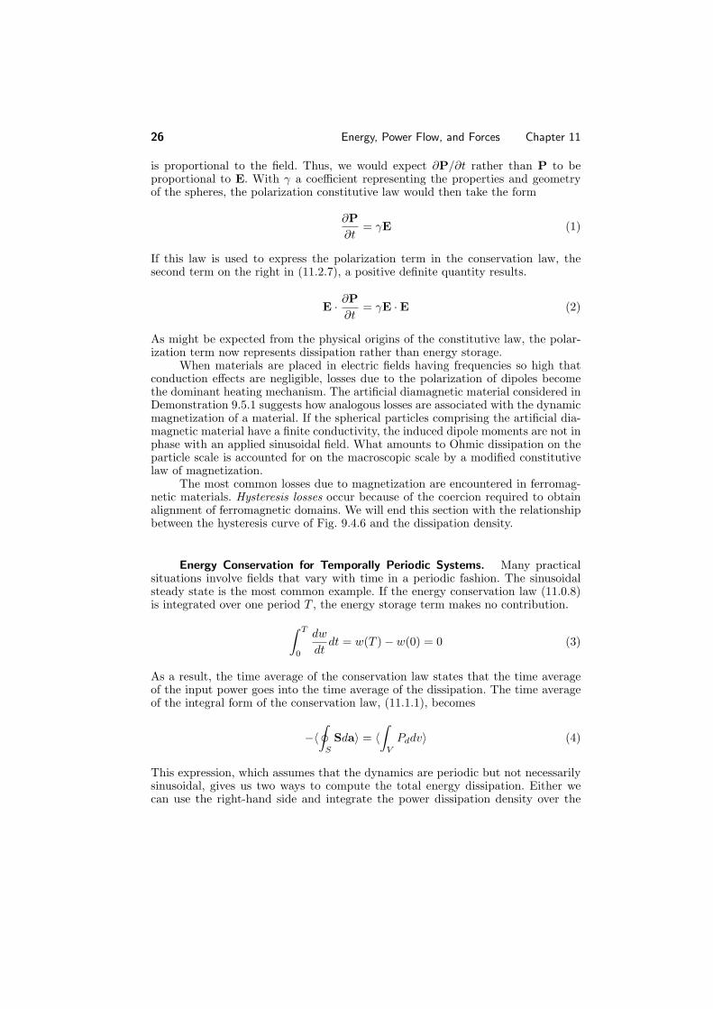
The thin conducting shell of Fig 1151 in a field Ho(t) applied collinear with its axis was described in Example 1031 Here the applied field is in the sinusoidal steady state
Ho = ReH oe
jωt (8)
According to (1039) the complex amplitude of the response the magnetic field inside the shell is
Hi = H
o (9)
1 + jωτm
28 Energy Power Flow and Forces Chapter 11
Fig 1151 Circular cylindrical conducting shell in imposed axial magnetic field intensity Ho(t)
where τm = 12microoσΔa
The complex amplitude of the surface current density circulating in the shell follows from (1038)
K = Ho + H
o =
jωτmH o
(10)minus 1 + jωτm
minus 1 + jωτm
Because the current density is uniform over the radial crossshysection of the shell the dissipation density can be written in terms of the surface current density K = ΔσE
K2
Pd = σE E = (11)middot Δ2σ
It follows from the application of the time average theorem (6) that the total time average dissipation is
Pddv =
1 Re
KKlowast
dv =2πaΔl
ReKKlowast (12) V
V
2 Δ2σ
2Δ2σ
where l is the shell length To complete the derivation based on an integration of the density over the volume of the conductor this expression can be evaluated using (10)
(ωτm)2 πal 2 pd equiv V
Pddv = po 1 + (ωτm)2
po equiv σΔ
|H o| (13)
The same result is found by evaluating the time average of the Poynting flux density integrated over a surface that is just outside the shell at r = a To see this we again use the time average theorem (6) and recognize that the surface integral amounts to a multiplication by the surface area of the shell
1 ˆ 2πal ˆminus
S
(Etimes H) middot da = S
2 ReEφHo
lowastda =2
ReEφHo lowast (14)
To evaluate this expression (10) is used to determine Eφ
K jωτmH o jωτm(1 minus jωτm)H
oEφ =
Δσ = minus
Δσ(1 + jωτm)= minus
Δσ[1 + (ωτm)2] (15)
Sec 115 Electromagnetic Dissipation 29
Fig 1152 Time average power dissipation density normalized to po
as defined with (13) as a function of the frequency normalized to the magnetic diffusion time defined with (9)
Evaluation of (14) then gives
(ωτm)2 πal
Etimes H da = po 1 + (ωτm)
po equiv σΔ
H o
2 (16)minus middot | |
which is the same result as found by integrating the dissipation density over the volume (13)
The dependence of the time average power dissipation on the normalized freshyquency is shown in Fig 1152 At very low frequencies the induced current is not large enough to have an appreciable effect on the imposed field Thus the electric field is proportional to the time rate of change of the applied field and because the dissipation is proportional to the square of E the power dissipation increases as the square of ω At high frequencies the induced current can be no more than that required to shield the imposed field from the region inside the shell As a result the dissipation reaches an asymptotic limit
Which of the two approaches is best for finding the total power dissipation The answer depends on what field information is available Certainly the notion that the total heat generated can be found by integrating over a surface that is completely outside the heated material is a fundamental consequence of Poyntingrsquos theorem
Dielectric Heating In the sinusoidal steady state we can identify the power dissipation density associated with polarization by finding the time average
partD Pd = E middot partt (17)
In view of the time average theorem (6) this becomes
1 Pd = 2RejωD middot Elowast (18)
If the polarization P does not follow the electric field E instantaneously yet the material is still linear and isotropic the complex vector P can be related to E by
30 Energy Power Flow and Forces Chapter 11
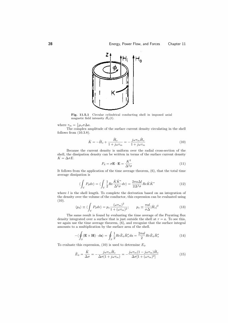
Fig 1153 Definition of angle δ defining the loss tangent tan(δ) in terms of the real and the negative of the imaginary parts of the complex permittivity
a complex susceptibility Or instead the complex displacement flux density vector D is related to E by a complex dielectric constant
D = E = ( minus j)E (19)
Here is the complex permittivity with real and imaginary parts and minus respecshytively
Evaluation of (18) using this constitutive law gives
Pd = ω
2|E| 2Rej =
ω
2|E| 2 (20)
Thus represents the electrical dissipation associated with the polarization proshycess
In the literature the loss tangent tan δ is often used to represent dissipation It is the tangent of the phase angle δ of the complex dielectric constant defined in terms and in Fig 1153 Thus
tan δ =
cos δ =
sin δ =
(21) | | | |
From this definition it follows from Eulers formula that
minus j = ||(cos δ minus j sin δ) = ||eminusjδ (22)
Given the complex amplitude of the electric field D is
D = Re||Eej(ωtminusδ) (23)
If the electric field is Eo cos(ωt) then D is ||Eo cos(ωtminus δ) The electric displaceshyment lags the electric field by the phase angle δ
In terms of the loss tangent defined by (21) the time average electrical dissishypation density of (20) becomes
Pd = ω
2
|E| 2 tan δ (24)
Usually the loss tangent and are measured In the following example we compute the complex permittivity from a model of the polarizable medium and
Sec 115 Electromagnetic Dissipation 31
find the electrical dissipation on a macroscopic basis In this special case we have the option of finding the time average loss by considering each of the dipoles on a microscopic basis This is not generally possible because the interactions among dipoles that are neglected in this example are usually too complicated for an analytic treatment
Example 1152 An Artificial Lossy Dielectric
By putting together examples considered in Chaps 6 and 7 we can illustrate the origins of the complex permittivity The artificial dielectric of Example 661 and Demonstration 661 had ldquomoleculesrdquo consisting of perfectly conducting spheres As a result the polarization was pictured as instantaneously in step with the applied field We consider now the result of having spheres that have finite conductivity
The response of a single sphere having a finite conductivity σ and permittivity surrounded by free space is a special case of Example 793 The response to a sinusoidal drive is summarized by (7936) where we set σa = 0 a = o σb = σ and b = All that is required from this solution for the potential is the moment of a dipole that would give rise to the same exterior field as does the sphere Comparison of the potential of a dipole (4410) to that given by (7936a) shows that the complex amplitude of the moment is
(minuso)
1 + jωτe 2o+
p = 4πoR3 E (25)
1 + jωτe
where τe equiv (2o + )σ If mutual interactions between dipoles are ignored the polarization density P is this moment of a single dipole multiplied by the number of dipoles per unit volume N For a cubic array with a distance s between the dipoles (the centers of the spheres) N = 1s3 Thus the complex amplitude of the electric displacement is
pD = oE + P = oE +
ˆ 3
(26) s
Combining this result with the moment given by (25) yields the desired constitutive
law in the form D = E where the complex permittivity is
= o
1 + 4π
R3 1 + jωτe
(2minuso
+o
)
(27) s 1 + jωτe
The time average power dissipation density follows from this expression and (20)
2πo R3
3o
(ωτe)
2
E 2 (28)Pd = τe s 2o + 1 + (ωτe)2
| |
The dependence of the power dissipation on frequency has the same form as for the induction heating example Fig 1152 At low frequencies the surface charges induced at the north and south poles of each sphere are completely determined by the external field Thus the current density within the sphere that makes possible the accumulation of these surface charges is proportional to the time rate of change of the applied field At low frequencies the dissipation is proportional to the square
32 Energy Power Flow and Forces Chapter 11
of the volume current and hence to the square of the time rate of change of the applied field As a result at low frequencies the dissipation density increases with the square of the frequency
As the frequency is raised less surface charge is induced on the spheres Alshythough the amount of charge induced is inversely proportional to the frequency there is a compensating effect because the volume currents are responsible for the dissipation and these are proportional to the time rate of change of the charge Thus the dissipation density reaches a saturation value as the frequency becomes very high
One tool used to form a picture of atomic molecular and domain physics is dielectric spectroscopy Using this approach the frequency dependence of the complex permittivity is used to gain insight into the microscopic structure
Magnetization like polarization can also be the source of dissipation The time average dissipation density due to magnetization follows by taking the time averge of the third and fourth terms on the right in the basic power theorem (1127) Combined these terms give
partB Pd = H middot partt (29)
For smallshysignal applications this source of dissipation is dealt with by inshytroducing a complex permeability ˆ micro such that B = microH The role of the complex permeability is similar to that of the complex permittivity The artificial diamagshynetic material of Example 952 and Demonstration 951 can be used to exemplify the concept Instead of perfectly conducting spheres that give rise to a magnetic moment instantaneously induced antiparallel to the applied field spherical shells of finite conductivity would be used The dipole moment induced in the individual spherical shells would be deduced following the same approach as in Sec 104 The resulting dipole moment would not be in phase with an applied sinusoidally varying magnetic field The derivation of an equivalent complex permeability would follow from the same line of reasoning as used in the previous example
Hysteresis Losses Under periodic conditions in magnetizable solids B and H are related by the hysteresis curve described in Sec 94 and illustrated again in Fig 1154 What time average power dissipation is implied by the hysteresis
As before B and H are collinear However neither is now a singleshyvalued function of the other Evaluation of (29) is accomplished by breaking the cycle into two parts each involving a singleshyvalued relationship between B and H The first is the upswing ldquotrajectoryrdquo from A C in Fig 1154 Over this halfshycycle which rarrtakes B from BA to BC the trajectory is H+(B) With B taken as BA when t = 0 it follows from (1144) and (1145) that
T2 partB BC dWm
BC
H dt = dt = H+δB (30) 0
middot partt BA
dt BA
This is the area under the curve of H versus B between A and C in Fig 1154 traversed on the ldquoupswingrdquo A similar evaluation for the ldquodownswingrdquo where the
Sec 116 Macroscopic Electrical Forces 33
Fig 1154 With the application of a sinusoidal magnetic field intensity a steady state is reached in which the hysteresis loop shown in the Bminus H plane is traced out in the direction shown The dashed area represents the energy density associated with upward traversal from A to C The dotted area inside the loop represents the energy density dissipated per traversal of the loop
trajectory is H (B) gives minus T partB
BA BC
H dt = H δB = H δB (31) T2
middot partt BC
minus minus BA
minus
The time average power dissipation (29) then is the sum of these two contributions divided by T
Pd =1 BC
H+δB minus BC
H δB
(32) T BA BA
minus
Thus the area within the hysteresis loop is the energy dissipated in one cycle
116 ELECTRICAL FORCES ON MACROSCOPIC MEDIA
Electrical forces on macroscopic materials have their origins in the forces exerted on the microscopic particles of which the materials are composed Macroscopic fields have been used to describe conduction polarization and magnetization In Chaps 6 7 and 9 polarization current and magnetization densities respectively were related to the macroscopic field variables through constitutive laws Typically the parameters in these laws are determined from measurements Thus the experimenshytally determined relations make it unnecessary to take detailed account of how the microscopic fields are averaged
Because the definition of the average is already implicit in our macroscopic formulation of Maxwellrsquos equations we must now take care that our use of macroshyscopic field quantities for representing electromagnetic forces is selfshyconsistent The
34 Energy Power Flow and Forces Chapter 11
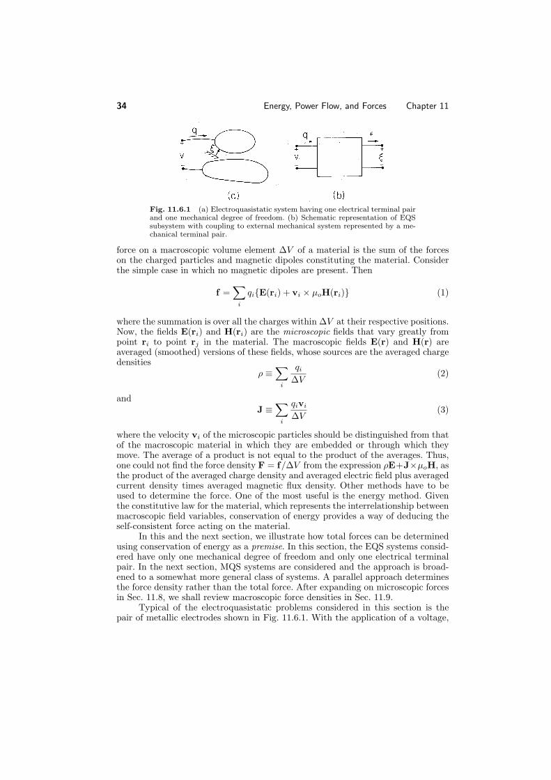
Fig 1161 (a) Electroquasistatic system having one electrical terminal pair and one mechanical degree of freedom (b) Schematic representation of EQS subsystem with coupling to external mechanical system represented by a meshychanical terminal pair
force on a macroscopic volume element ΔV of a material is the sum of the forces on the charged particles and magnetic dipoles constituting the material Consider the simple case in which no magnetic dipoles are present Then
f =
qiE(ri) + vi times microoH(ri) (1) i
where the summation is over all the charges within ΔV at their respective positions Now the fields E(ri) and H(ri) are the microscopic fields that vary greatly from point ri to point rj in the material The macroscopic fields E(r) and H(r) are averaged (smoothed) versions of these fields whose sources are the averaged charge densities
ρ equiv
Δq
V i (2)
i
and J equiv
qivi (3)ΔV
i
where the velocity vi of the microscopic particles should be distinguished from that of the macroscopic material in which they are embedded or through which they move The average of a product is not equal to the product of the averages Thus one could not find the force density F = fΔV from the expression ρE+JtimesmicrooH as the product of the averaged charge density and averaged electric field plus averaged current density times averaged magnetic flux density Other methods have to be used to determine the force One of the most useful is the energy method Given the constitutive law for the material which represents the interrelationship between macroscopic field variables conservation of energy provides a way of deducing the selfshyconsistent force acting on the material
In this and the next section we illustrate how total forces can be determined using conservation of energy as a premise In this section the EQS systems considshyered have only one mechanical degree of freedom and only one electrical terminal pair In the next section MQS systems are considered and the approach is broadshyened to a somewhat more general class of systems A parallel approach determines the force density rather than the total force After expanding on microscopic forces in Sec 118 we shall review macroscopic force densities in Sec 119
Typical of the electroquasistatic problems considered in this section is the pair of metallic electrodes shown in Fig 1161 With the application of a voltage
Sec 116 Macroscopic Electrical Forces 35
unpaired charges of opposite polarity are induced on the electrode surfaces The electrical state of the system is specified by giving the geometry and the potential difference v between the electrodes Here we picture one electrode as movable with its position denoted by ξ The two terminal pair system of Fig 1161b is useful to include mechanical effects via an additional terminal pair If we think of the net unpaired charge q on the electrode as an electrical terminal variable complementing v then the force of electrical origin f complements the mechanical displacement ξ
Given the electrical terminal relation v = v(q ξ) we now use an energy conshyservation principle to determine the force f = f(q ξ) that acts to increase the displacement ξ The electrical terminal relation can either be regarded as a meashysured function or be predicted using the macroscopic field laws and constitutive laws for the materials within the ldquoboxrdquo
It is now assumed that there is no conversion of electrical energy to thermal form within the box of Fig 1161b Mechanisms for conversion of energy to heat are modeled by elements outside the box For example the finite conductivity of any dielectric is taken into account by a resistance external to the system Thus the electrical power input to what is defined as the ldquoboxrdquo the electroquasistatic subsystem must either result in a change in the electrical energy stored or mechanshyical power expended as the force f acts on the mechanical system The integral form of the power conservation theorem (1111) is generalized to include the rate of work by the force f
S da =
d
Wedv + f dξ
(4)minus S
middot dt V dt
In Sec 114 we represented the quasistatic net electrical power input on the left in this expression in circuit theory terms With the total energy we defined as the integral of the energy density over the entire volume of the system (4) becomes
vdq
= dwe + f
dξ (5)
dt dt dt
where the electrical power input is the product vi = vdqdt Multiplication of (4) by dt converts a statement of power flow to one of energy conservation
vdq = dwe + fdξ (6)
If an increment of charge dq is placed on an electrode at potential v an increment of energy vdq is added to the system that produces a change in the total stored energy dwe an increment of work fdξ done on an external mechanical system or some combination of both Here f(q ξ) is the as yet unknown force Solved for dwe this energy conservation statement is
dwe = vdq minus fdξ (7)
This expression describes what might be termed a quasistatic electrical and mechanshyical subsystem The state of this subsystem is specified by prescribing the geometry (ξ) and the charge on the electrode for then the voltage of the electrode follows
36 Energy Power Flow and Forces Chapter 11
Fig 1162 Path of line integration in state space (q ξ) used to find energy at location C
from the terminal relation v(q ξ) The state of the subsystem is fully determined by the variables (q ξ) which are therefore regarded as independent variables In terms of the two terminal pairs shown in Fig 1161b one of each pair of terminal variables has been chosen as an independent variable
The incremental change in we(q ξ) associated with incremental changes of dq and dξ in the independent variables is
dwe = partwe
dq + partwe
dξ (8)partq partξ
Because q and ξ can be independently specified (7) and (8) must hold for any combination of dq and dξ For example they must hold if the position of the electrode is held fixed so that dξ = 0 and the charge is changed by the incremental amount dq They must also describe the change in energy resulting from making an incremental displacement dξ of the electrode under open circuit conditions where dq = 0 Indeed (7) and (8) hold if q and ξ are changed by arbitrary incremental amounts and so it follows that the coefficients of dq in (7) and (8) must be equal to each other as must the coefficients of dξ
part part v =
partq we(q ξ) f = minus
partξ we(q ξ)
(9)
Given the total energy written in terms of the independent variables (q ξ) the second of these relations provides the desired force Integration of the energy density over the volume of the system is one way to determine we Another is to integrate (7) along a line in the state space (q ξ) designed so that the integral can be carried out without having to know f
we(q ξ) = (vdq minus fdξ) (10)
Such a path4 is shown in Fig 1162 where it is assumed that the force of electrical origin f is zero if the charge q is zero Thus in integrating along the contour q = 0 from A B dq = 0 and f = 0 so there is no contribution The remainder of the integral from
rarrB C is carried out with ξ fixed so dξ = 0 and
(10) reduces to rarr
4 Note the analogy with the line integral
(Exdx +Eydy) of a twoshydimensional conservation
field that results in the potential φ(x y)
Sec 116 Macroscopic Electrical Forces 37
ξ q q
we = f(0 ξ)dξ + v(q ξ)dq = v(q ξ)dqminus 0 0 0 (11)
We have accounted for the energy required to place the subsystem in the state (q ξ) In physical terms the mathematical steps represent first assembling the subsystem mechanically with no electrical excitation Because there is no force acting on the electrode as it is put in place no work is involved Then with its location fixed the electrode is charged by means of an electrical source
Suppose that the subsystem is electrically linear so that either as a result of mathematical modeling or of measurements on the actual system the electrical terminal relation takes the form
q v = (12)
C(ξ)
Then with this relation used to evaluate (11) it follows that the energy is
2 q q 1 q we = dq = (13)
C 2 C0
Finally the desired force of electrical origin follows from substituting this expression into (9b)
1 2 dCminus1
f = 2qminus
dξ =
1 q 2 dC
2 C dξ (14)
Note that with a similar substitution into (9a) the terminal relation of (12) is obtained
Once the partial derivative with respect to ξ has been taken while holding the proper independent variable (q) fixed the force can be written in terms of variables other than the independent ones Thus with the use of the terminal relation (12) the force is written in terms of the terminal voltage v as
1 2 dC f = v
2 dξ (15)
The following example gives the opportunity to apply this result to a specific configuration
Example 1161 Force on a Capacitor Plate
The region between the plane parallel electrodes shown in Fig 1163 is filled by a layer of dielectric having permittivity and thickness b and an air gap ξ The total distance between electrodes b + ξ is small compared to the linear dimensions of the plates so fringing fields will be ignored Thus the electric fields Ea and Eb in the air gap and in the dielectric respectively are uniform What force on the upper electrode results from applying the voltage v between the electrodes
38 Energy Power Flow and Forces Chapter 11
Fig 1163 Specific example of EQS systems having one electrical and one mechanical terminal pair
First we determine the charge q on the upper electrode To this end the integral of E from the upper electrode to the lower one must be equal to the applied voltage so
v = ξEa + bEb (16)
Further there is presumably no unpaired surface charge at the interface between the dielectric layer and the air gap Thus Gaussrsquo continuity condition requires that
oEa = Eb (17)
Elimination of Eb between these equations gives
Ea = v
(18)ξ + b o
In terms of this electric field at the surface of the upper electrode Gaussrsquo continuity condition shows that the total charge on the upper electrode is
q = DaA = oEaA (19)
and so it follows from (18) that the electrical terminal relation can be written in terms of a capacitance C
oA q = Cv C equiv (20)
ξ + b o
Because the dielectric is described by a linear constitutive law we have obtained an electrical terminal relation where v is a linear function of q
The force acting on the upper electrode follows from a substitution of (20) into (15)
1 2 oA f = v (21)minus
2 ξ
2 + b o
By definition if f is positive it acts in the direction of ξ Here we find that regardless of the polarity of the applied voltage f is negative This is to be expected because charges of one polarity on the upper electrode are attracted toward those of opposite polarity on the lower electrode
In describing energy conversion a minus sign can be extremely important For example vdq is the incremental energy into the electroquasistatic subsystem while fdξ is the energy leaving that subsystem as the force of electrical origin acts on the external mechanical system Thus if f is positive it acts on the mechanical system in such a direction as to increase the associated displacement
Sec 116 Macroscopic Electrical Forces 39
Fig 1164 Apparatus used to demonstrate amplification of voltage as the upper electrode is raised (The electrodes are initially charged and then the voltage source is removed so q = constant) The electrodes consisting of foil mounted on insulating sheets are about 1 m times 1 m with the upper one insulated from the frame which is used to control its position The voltage is measured by the electrostatic voltmeter which ldquoloadsrdquo the system with a capacitance that is small compared to that of the electrodes and (at least on a dry day) a negligible resistance
Rotating motors and generators are examples where the conversion of energy between electrical and mechanical form is a cyclic process In these cases the subshysystem returns to its original state once each cycle The energy converted per cycle is determined by integrating the energy conservation law (6) around the closed path in the state space representing this process
vdq = dwe + fdξ (22)
Because the energy stored in the system must return to its original value there is no net contribution of the energy storage term in (22) For a cyclic process the net electrical energy input per cycle must be equal to the net mechanical power output per cycle
vdq = fdξ (23)
The following demonstration is primarily intended to give further insight into the implications of the conservation of energy principle for a cyclic process
Demonstration 1161 An Energy Conversion Cycle
The experiment shown in Fig 1164 is based on the plane parallel capacitor conshyfiguration analyzed in Example 1161 The lower electrode aluminum foil mounted on a table top is covered by a thin sheet of plastic The upper one is also foil but taped to an insulating sheet which is attached to a frame This electrode can then be manually raised and lowered to effectively control the displacement ξ
With the letters A through D used to designate states of the system we consider the following energy conversion cycle
bull A B With v = 0 the upper electrode rests on the plastic sheet A voltage Vo
rarris applied
B C With the voltage source removed so that the upper electrode isbull rarrelectrically isolated it is raised to the position ξ = L
bull C D The upper electrode is shorted so that its voltage returns to zero Drarr
A The upper electrode is returned to its original position at ξ = 0bull rarr
40 Energy Power Flow and Forces Chapter 11
Fig 1165 Closed paths followed in cyclic conversion of energy from mechanical to electrical form (a) in (q v) plane and (b) in (f ξ) plane
Is electrical energy converted to mechanical form or vice versa The process in carrying out the closed integrals on the leftshyhand and rightshy
hand sides of (23) as the cycle is carried out can be pictured in the (q v) and (f ξ) planes respectively as shown in Fig 1165 From A B q = C(0)v where C(ξ)rarris given by (20) Thus the trajectory in the (q v) plane is a straight line ending at the voltage v = Vo of the source Because the upper electrode has remained at its original position the trajectory in the (f ξ) plane is along the ξ = 0 axis The force on the electrode caused by raising its voltage to Vo follows from (21)
1 v 2C2 1 [VoC(0)]2 f = fB = (24)minus
2 oA rArr minus
2 oA
Now from B C the voltage source is removed so that as the upper electrode rarris raised to ξ = L its charge is conserved This means that the trajectory in the (q v) plane is one where q = constant = VoC(0) The voltage reached by the upper electrode can be found by requiring that q be conserved
C(0)VoC(0) = V C(L) V = Vo (25)rArr
C(L)
In the experiment the thickness b of the dielectric sheet is a fraction of a millimeter while the final elevation ξ = L might be 20 cm (If the displacement is larger than this the fringing field comes into play and the expression for the capacitance is no longer valid) Thus as the sheet is raised an original voltage of 500 V is easily amplified to 10 shy 20 kV This is readily observed by means of an electrostatic voltmeter attached to the upper electrode as shown in Fig 1164
To determine the trajectory B C in the (f ξ) plane observe from (14) or rarr(24) that as a function of q the force is independent of ξ
1 q 2 f = minus
2 oA (26)
The trajectory B C in the (f ξ) plane is therefore one of constant fB given by rarr(24) In general f(q ξ) is not independent of ξ but in plane parallel geometry it is
The system is now returned to its original state in two steps First from C D the upper electrode remains at ξ = L and is shorted to ground In the (q v)rarrplane the state returns to the origin along the straight line given by q = C(L)v (20) In the (f ξ) plane the force drops to zero with ξ = L Second from D Ararr
Sec 116 Macroscopic Electrical Forces 41
the upper electrode is returned to its original position The values of (q v) remain zero while the trajectory in the (f ξ) plane is f = 0
The experiment is simple enough so that we can use physical reasoning to decide the direction of energy conversion Although the force of gravity is likely to exceed the electrical force of attraction between the electrodes as far as the electrical subsystem is concerned the upper electrode is raised against a downward electrical force Because the charge is removed before it is lowered there is no electrical force on the electrode as it is lowered Thus net work is done on the EQS subsystem The rightshyhand side of (23) the net work done by the subsystem on the external mechanical system is thus negative
2
Evaluation of one or the other of the two sides of the energy conversion law (23) provides two other ways to determine the direction of energy conversion Conshysider first the electrical input energy The integral has contributions from A Brarr(where the source is used to charge the upper electrode) and from C D (whererarrthe electrode is discharged) The areas under the respective triangles representing the integral of vdq are
C(0)Vo
B D 1 1 2vdq vdq + vdq C(L)V (27)
2
minus 2
C(0)Vo
= = 2
2
A C
C(0)Vo
In view of the expression for C(ξ) (20) this expression can be written as
C(0)
1 1 L
vdq 1minus (28)minus 2
= = 2 C(L) b o
22
This expression is clearly negative indicating that the net electrical energy flow is out of the electrical terminal pair This is consistent with having a net mechanical energy input to the system
The net mechanical output energy per cycle expressed by the rightshyhand side of (23) should be equal to (28) To see that this is so we recognize that the integral consists of two possible contributions from B C and D A During the latter rarr rarrf = 0 so the magnitude of the integral is simply the area of the rectangle in Fig 1165b
Vo C(0)Vo C2(0)1 1 L
fdξ L (29)minus 2
minus 2
= = oA b o
As required by the conservation law this mechanical energy output is negative and is equal to the net electrical input energy given by (28)
With the sequence of electrical and mechanical terminal constraints described above there is a net conversion of energy from mechanical to electrical form The system acts as an electrical generator with energy provided by whoever raises and lowers the upper electrode With the voltage applied when the electrode is at its largest displacement and the electrode grounded before it is raised the energy flow is from the electrical voltage source to the mechanical system In this case the system acts as a motor We will have the opportunity to exemplify a practical motor in the next section Most motors are MQS rather than EQS However a practical EQS device that is designed to convert energy from mechanical to electrical form is the capacitor microphone a version of which was described in Example 633
Electrical forces have their origins in forces on unpaired charges and on dipoles The force on the upper capacitor plate of Example 1161 is due to the unpaired charges The equal and opposite force on the combination of electrode and dielectric
42 Energy Power Flow and Forces Chapter 11
Fig 1166 Slab of dielectric partially extending between capacitor plates The spacing a is much less than either b or the depth c of the system into the paper Further the upper surface at ξ is many spacings a away from the upper and lower edges of the capacitor plates as is the lower surface as well
is in part due to unpaired charges and in part to dipoles induced in the dielectric The following exemplifies a total force that is entirely due to polarization
Example 1162 Force on a Dielectric Material
We return to the configuration of Example 1141 where a dielectric slab extends a distance ξ into the region between plane parallel electrodes as shown in Fig 1166 The capacitance was found in Example 1141 to be (11416)
c C = [ob + ξ(minus o)] (30)
a
It follows from (15) that there is a force tending to draw the dielectric into the region between the electrodes
1 2 cf = v (minus o) (31)2 a
This force results because dipoles induced by the fringing field experience forces in the ξ direction that are passed on to the material in which they are embedded Even though the force is due to the fringing fields the net force does not depend on the details of that field This is evident from our energy arguments because at least as long as the upper edge of the slab is well within the region between the plates and the lower edge never reaches the vicinity of the electrodes the energy storage in the fringing fields does not change when the slab is moved
Further discussion of the force density responsible for the force on the dielectric will be given in Sec 119 Its physical reality is demonstrated next
Demonstration 1162 Force on a Liquid Dielectric
In the experiment shown in Fig 1167 capacitor plates are dipped into a dish full of dielectric liquid Thus with the application of the voltage it rises against gravity To demonstrate the relationship between the voltage and the force the spacing between the electrodes is a slowly varying function of radial position With r denoting the radial distance from an axis where an extension of the electrodes would join and α
Sec 116 Macroscopic Electrical Forces 43
Fig 1167 In a demonstration of the polarization force a pair of conducting transparent electrodes are dipped into a liquid (corn oil dyed with food coloring) They are closer together at the upper right than at the lower left so when a voltage is applied the electric field intensity decreases with increasing distance r from the apex As a result the liquid is seen to rise to a height that varies as 1r2 The electrodes are about 10 cm times 10 cm with an electric field exceeding the nominal breakdown strength of air at atmospheric pressure 3 times 106 Vm The experiment is therefore carried out under pressurized nitrogen
the angle between the electrodes the spacing at a distance r is αr Thus in (31) the spacing between electrodes a αr and the force per unit radial distance tendingrarrto push the liquid upward is a function of the radial position
f 1 v 2 = (minus o) (32)
c 2 αr
This force must raise a column of liquid having a height ξ and width αr With the mass density of the liquid defined as ρ the total mass per radial distance raised by this force is therefore αrξρ Force equilibrium is therefore represented by setting the force per unit radial length equal to this mass multiplied by the gravitational acceleration g
1 v 2 (minus o) = αrξρg (33)
2 αr
This expression can be solved for ξ(r)
1 v 2(minus o) 1 ξ = (34)
2 α2ρg r2
In the experiment5 the electrodes are constructed from tinshyoxide coated glass They are then both conducting and transparent As a result the height to which the liquid rises can be seen to obey (34) both as to its magnitude and its radial dependence on r
5 See film Electric Fields and Moving Media from series by National Committee for Electrical Engineering Films Education Development Center 39 Chapel St Newton Mass 02160
44 Energy Power Flow and Forces Chapter 11
Fig 1171 (a) Magnetoquasistatic system with two electrical terminal pairs and one mechanical degree of freedom (b) MQS subsystem representing (a)
To obtain an appreciable rise of the liquid without exceeding the field strength for electrical breakdown between the electrodes the atmosphere over the liquid must be pressurized Also to avoid effects of unpaired charges injected at high field strengths by the electrodes the applied voltage is alternating and because the force is proportional to the square of the applied field the height of rise is proportional to the rms value of the voltage
117 MACROSCOPIC MAGNETIC FORCES
In this section an energy principle is applied to the determination of net forces in MQS systems With Sec 116 as background it is appropriate to include the case of multiple terminal pairs As in Sec 114 the coenergy is again found to be a convenient alternative to the energy
The MQS system is shown schematically in Fig 1171 It has two electrical terminal pairs and one mechanical degree of freedom The magnetoquasistatic subshysystem now described by an energy principle excludes electrical dissipation and all aspects of the mechanical system mechanical energy storage and dissipation The energy principle then states that the input of electrical power through the electrical terminal pairs either goes into a rate of change of the stored magnetic energy or into a rate of change of the work done on the external mechanical world
v1i1 + v2i2 = dwm + f
dξ (1)
dt dt
As in Sec 116 our starting point in finding the force is a postulated principle of energy conservation Because the system is presumably MQS in accordance with (11329) the leftshyhand side represents the net flux of power into the system With the addition of the last term and the inherent assumption that there is no electrical dissipation in the subsystem being described (1) is more than the recasting of Poyntingrsquos theorem
In an MQS system the voltages are the time rates of change of the flux linkages With these derivatives substituted into (1) and the expression multiplied by dt it becomes
Sec 117 Macroscopic Magnetic Forces 45
i1dλ1 + i2dλ2 = dwm + fdξ (2)
This energy principle states that the increments of electrical energy put into the MQS subsystem (as increments of flux dλ1 and dλ2 through the terminals multiplied by their currents i1 and i2 respectively) either go into the total energy which is increased by the amount dwm or into work on the external mechanical system subject to the force f and experiencing a displacement dξ
With the energy principle written as in (2) the flux linkages are the indepenshydent variables We saw in Example 1142 that it is inconvenient to specify the flux linkages as functions of the currents With the objective of casting the currents as the independent variables we now recognize that
i1dλ1 = d(i1λ1)minus λ1di1 i2dλ2 = d(i2λ2)minus λ2di2 (3)
and substitute into (2) to obtain
dw = λ1di1 + λ2di2 + fdξ (4)m
where the coenergy function seen before in Sec 114 is defined as
w = (5)m i1λ1 + i2λ2 minus wm
We picture the MQS subsystem as having flux linkages λ1 and λ2 a force f and a total energy wm that are specified once the currents i1 and i2 and the displacement ξ are stipulated According to (4) the coenergy is a function of the independent variables i1 i2 and ξ wm = m(i1 i2 ξ) and the change in w can w m also be written as
partw partw m partw dw = m di1 +
di2 + m dξ (6)m parti1 parti2 partξ
Because the currents and displacement are independent variables (4) and (6) can hold only if the coefficients of like terms on the right are equal Thus
partw partw partw λ1 = m λ2 = m f = m
parti1 parti2 partξ (7)
The last of these three expressions is the key to finding the force f
Reciprocity Condition Before we find the coenergy and hence f consider the implication of the first two expressions in (7) for the electrical terminal relations Taking the derivative of λ1 with respect to i2 and of λ2 with respect to i1 shows that
partλ1 = part2w
= part2w
= partλ2m m
parti2 parti1parti2 parti2parti1 parti1 (8)
46 Energy Power Flow and Forces Chapter 11
Although this reciprocity condition must reflect conservation of energy for any lossshyless system magnetically linear or not consider its implications for a system deshyscribed by the linear terminal relations
λ1
=
L11 L12
i1
(9)λ2 L21 L22 i2
Application of (8) shows that energy conservation requires the equality of the mushytual inductances
L12 = L21 (10)
This relation has been derived in Example 1142 from a related but different point of view
Finding the Coenergy To find w we integrate (4) along a path in the state mspace (i1 i2 ξ) arranged so that the integral can be carried out without having to know f
w = (λ1di1 + λ2di2 + fdξ)m(11)
Thus the first leg of the line integral is carried out on ξ with the currents equal to zero Provided that f = 0 in the absence of these currents this means that the integral of fdξ makes no contribution
The payoff from our formulation in terms of the coenergy rather than the energy comes in being able to carry out the remaining integration using terminal relations in which the flux linkages are expressed in terms of the currents For the linear terminal relations of (9) this line integration was illustrated in Example 1142 where it was found that
1 1 w = L11i
2 + L12i1i2 + L22i2 (12)m 1 22 2
Evaluation of the Force In general the inductances in this expression are functions of ξ Thus the force f follows from substituting this expression into (7c)
1 dL11 dL12 1 dL22f =
2i21 dξ
+ i1i2 dξ
+2i22 dξ (13)
Of course this expression applies to systems having a single electrical terminal pair as a special case where i2 = 0
This generalization of the energy method to multiple electrical terminal pair systems suggests how systems with two or more mechanical degrees of freedom are treated
Sec 117 Macroscopic Magnetic Forces 47
Fig 1172 Crossshysection of axially symmetric transducer similar to the ones used to drive dot matrix printers
Example 1171 Driver for a Matrix Printer
A transducer that is similar to those used to drive an impact printer is shown in Fig 1172 The device which is symmetric about the axis might be one of seven used to drive wires in a highshyspeed matrix printer The objective is to transduce a current i that drives the N shyturn coil into a longitudinal displacement ξ of the permeable disk at the top This disk is attached to one end of a wire the other end of which is used to impact the ribbon against paper imprinting a dot
The objective here is to determine the force f acting on the plunger at the top For simplicity we make a highly idealized model in which the magnetizable material surrounding the coil and filling its core as well as that of the movable disk is regarded as perfectly permeable Moreover the air gap spacing ξ is small compared to the radial dimension a so the magnetic field intensity is approximated as uniform in the air gap The wire is so fine that the magnetizable material removed to provide clearance for the wire can be disregarded
With Ha and Hc defined as shown by the inset to Fig 1172 Amperersquos integral law is applied to a contour passing upward through the center of the core across the air gap at the center radially outward in the disk and then downward across the air gap and through the outer part of the stator to encircle the winding in the infinitely permeable material
Haξ + Hcξ = Ni (14)
A second relation between Ha and Hc follows from requiring that the net flux out of the disk must be zero
microoHaπ(a 2 minus b2) = microoHcπc 2 (15)
Using this last expression to replace Hc in (14) results in
Ni Hc = 2 (16)
cξ1 +
a2minusb2
48 Energy Power Flow and Forces Chapter 11
Fig 1173 Crossshysection of perfectly conducting currentshycarrying wire over a perfectly conducting ground plane
The magnetic flux linking every turn in the coil is microoHcπc2 Thus the total flux linked by the coil is
microoN2πc2
λ = Li L = 2 (17)cξ
1 +
a2minusb2
Finally the force follows from an evaluation of (13) (specialized to the single terminal pair system of this example)
1 2 dL 1 2 microoN2πc2
f = i = ic2
(18)2 dξ
minus 2 ξ2
1 +
a minusb2
2
As might have been expected by one who has observed magnetizable materials pulled into a magnetic field the force is negative Given the definition of ξ in Fig 1172 the application of a current will tend to close the air gap To write a dot the current is applied To provide for a return of the plunger to its original position when the current is removed a spring is inserted in the air gap
In the magnetic transducer of the previous example the force on the driver disk is due to magnetization The next example illustrates the force associated with the current density
Example 1172 Force on a Wire over a Perfectly Conducting Plane
The crossshysection of a perfectly conducting wire with its center a distance ξ above a perfectly conducting ground plane is shown in Fig 1173 The configuration is familiar from Demonstration 861 The current carried by the wire is returned in the ground plane The distribution of this current on the surfaces of the wire and ground plane is consistent with the requirement that there be no flux density normal to the perfectly conducting surfaces What is the force per unit length f acting on the wire
The inductance per unit length is half of that for a pair of conductors having the centershytoshycenter spacing 2ξ Thus it is half of that given by (8612)
microo
ξ
ξ 2 minus 1
L = ln + (19)
2π R R
Sec 117 Macroscopic Magnetic Forces 49
Fig 1174 The force tending to levitate the wire of Fig 1173 as a function of the distance to the ground plane normalized to the radius R of wire
The force per unit length in the ξ direction then follows from an evaluation of (13) (again adapted to the single terminal pair situation)
1 2 dL 1 microoi2
f = i = fo fo = (20)2 dξ
(ξR)2 minus 1 4πR
The dependence of this force on the elevation above the ground plane is shown in Fig 1174 In the limit where the elevation is large compared to the radius of the conductor (20) becomes
1 microoi2
f (21)rarr 4 πξ
In Sec 118 we will identify the force density acting on materials carrying a current density J as being J times microoH Note that the upward force predicted by (20) is indeed consistent with the direction of this force density
The force on a thin wire (21) can be derived from this force density by recognizing that the contribution of the selfshyfield of the wire to the total force per unit length is zero Thus the force per unit length can be computed using for B the flux density caused by the image current a distance 2ξ away The flux density due to this image current has a magnitude that follows from Amperersquos integral law as microoi2π(2ξ) This field is essentially uniform over the crossshysection of the wire so the integral of the force density Jtimes B over the crossshysection of the wire amounts to an integration of the current density J over the crossshysection The latter is the total current i and so we are led to a force per unit length of magnitude microoi
22π(2ξ) which is in agreement with (21)
The following is a demonstration of the force on currentshycarrying conductors exemplified previously It also provides a dramatic demonstration of the existence of induced currents
Demonstration 1171 Steady State Magnetic Levitation
In the experiment shown in Fig 1175 the currentshycarrying wire of the previous example has been wound into a pancake shaped coil that is driven by about 20 amps of 60 Hz current The conductor beneath is an aluminum sheet of 13 cm thickness Even at 60 Hz this conductor tends to act as a perfect conductor This follows from
50 Energy Power Flow and Forces Chapter 11
Fig 1175 When the pancake coil is driven by an ac current it floats above the aluminum plate In this experiment the coil consists of 250 turns of No 10 copper wire with an outer radius of 16 cm and an inner one of 25 cm The aluminum sheet has a thickness of 13 cm With a 60 Hz current i of about 20 amp rms the height above the plate is 2 cm
Fig 1176 (a) The force f acting through a levershyarm of length r produces a torque τ = rf (b) Mechanical terminal pair representing a rotational degree of freedom
an evaluation of the product of the angular frequency ω and the time constant τm
estimated in Sec 102 From (10217) ωτm = ωmicrooσΔa asymp 20 where the average radius is a = 9 cm Δ is the sheet thickness and the sheet conductivity is given by Table 711
The time average force of the type described in Example 1172 is sufficiently large to levitate the coil As the current is increased its height above the aluminum sheet increases as would be expected from the dependence of the force on the height for a single wire Fig 1174
The Torque of Electrical Origin In some of the most important transducers the mechanical response takes the form of a rotation rather than a translation The shaft shown in Fig 1176a might be attached to the rotor of a motor or generator A force f acting through a lever arm of length r that rotates the shaft through an incremental angle dθ causes a displacement dξ = rdθ Thus the incremental work done on the mechanical system fdξ becomes
fdξ τdθ (22)rarr
where τ is defined as the torque If the two terminal pair MQS system of Fig 1171 had a rotational rather
than a displacement degree of freedom the representation would be the same as has been outlined except that f τ and ξ θ The mechanical terminal pair is now represented as in Fig 1176b
rarr rarr
Sec 117 Macroscopic Magnetic Forces 51
Fig 1177 Crossshysection of rotating machine
The torque follows from (13) as
τ =1 i21
dL11 + i1i2 dL12 +
1 i22
dL22 (23)2 dθ dθ 2 dθ
Among the types of magnetic rotating motors and generators that could be used to exemplify the torque of (23) we now choose a synchronous machine Alshythough other types of motors are more common it is a near certainty that if these words are being read with the aid of electrical illumination the electricity used is being generated by means of a synchronous generator
Example 1173 A Synchronous Machine
The crossshysection of a stator and rotor modeling a rotating machine is shown in Fig 1177 The rotor consists of a highly permeable circular cylindrical material mounted on a shaft so that it can undergo a rotation measured by the angle θ Surrounding this rotor is a stator composed of a highly permeable material In slots on the inner surface of the stator and on the outer surface of the rotor respectively are windings with sinusoidally varying turn densities These windings driven by the currents i1 and i2 respectively give rise to current distributions that might be modeled by surface current densities
Kz = i1Ns sin φ at r = a (24)
Kz = i2Nr sin(φminus θ) at r = b (25)
where Ns and Nr are constants descriptive of the windings Thus the current disshytribution shown on the stator in Fig 1177 is fixed and gives rise to a magnetic field having the fixed vertical axis shown in the figure The rotor coil gives rise to a similar field except that its axis is at the angle θ of the rotor The rotor magnetic axis also shown in Fig 1177 therefore rotates with the rotor
Electrical Terminal Relations With the rotor and stator materials taken as infinitely permeable the air gap fields are determined by using (24) and (25) to
52 Energy Power Flow and Forces Chapter 11
write boundary conditions on the tangential H and then solving Laplacersquos equation for the air gap magnetic fields (Secs 96 and 97) The flux linked by the respective coils is then of the form
λ1
=
L11 L12(θ)
i1
λ2 L12(θ) L22 i2
Ls M cos θ
i1 (26)
= M cos θ Lr i2
where the selfshyinductances Ls and Lr and peak mutual inductance M are constants The dependence of the inductance matrix on the angle of the rotor θ can be
reasoned physically The rotor is modeled as a smooth circular cylinder so in the absence of a rotor current i2 there can be no effect of the rotor angle θ on the flux linked by the stator winding Hence the stator selfshyinductance is independent of θ Similar reasoning shows that the rotor selfshyinductance must be independent of rotor angle θ The θ dependence of the mutual inductance is plausible because the flux λ1
linked by the stator due to the current in the rotor must peak when the magnetic axes of the coils are aligned (θ = 0) and must be zero when they are perpendicular (θ = 90 degrees)
Torque Evaluation The magnetic torque on the rotor follows directly from using (26) to evaluate (23)
d τ = i1i2 M cos θ = minusi1i2M sin θ (27)
dθ
This torque depends on the currents and θ in such a way that the magnetic axis of the rotor tends to align with that of the stator With θ = 0 the axes are aligned and there is no torque If θ is slightly positive and the currents are both positive the torque is negative This is as would be expected with the magnetic axis of the stator vertical and that of the rotor in the first quadrant (as in Fig 1177)
Synchronous Operation In the synchronous mode of operation the stator current is constrained to be sinusoidal while that on the rotor is a constant To avoid having to describe the mechanical system we will assume that the shaft is attached to a mechanical load that makes the angular velocity Ω constant Thus the electrical and mechanical terminals are constrained so that
i1 = I1 cos ωt
i2 = I2 (28)
θ = Ωt minus γ
Under what circumstances can we derive a time average torque on the shaft and hence a net conversion of energy with each rotation
With the constraints of (28) the torque follows from (27) as
τ = minusI1I2M cos ωt sin(Ωt minus γ) (29)
Sec 117 Macroscopic Magnetic Forces 53
Fig 1178 (a) Time average torque as a function of angle γ (b) The rotor magnetic axis lags the clockwise rotating component of the stator magnetic field axis by the angle γ
A trigonometric identity6 makes the implications of this result more apparent
τ = minus I1I
2 2M
sin[(ω + Ω)t minus γ] + sin[minus(ω minus Ω)t minus γ]
(30)
There is no time average value of either of these sinusoidal functions of time unless one or the other of the frequencies (ω + Ω) and (ωminus Ω) is zero For example with the rotation frequency equal to that of the excitation
ω = Ω (31)
the time average torque is
I1I2M τ = sin γ (32)2
The dependence of the time average torque on the phase angle γ is shown in Fig 1178a With γ between 0 and 180 degrees there is a positive time average torque acting on the external mechanical system in the direction of rotation Ω In this range the machine acts as a motor to convert energy from electrical to mechanical form In the range of γ from 180 degrees to 360 degrees energy is converted from mechanical to electrical form and operation is as a generator
Stator Field Analyzed into Traveling Waves From (30) it is clear that a timeshyaverage torque results from either a forward (Ω = ω) or a backward (Ω = minusω) rotation This suggests that the field produced by the stator winding is the superposition of fields having magnetic axes rotating in the clockwise and counterclockwise directions Formally this can be seen by rewriting the stator surface current density (24) using the electrical and mechanical constraints of (28) With the use once again of the doubleshyangle trigonometric identity the distribution of surface current density is separated into two parts
NsI1Kz = NsI1 cos ωt sin φ = [sin(φ + ωt) + sin(φminus ωt)] (33)
2
6 sin(x) cos(y) = 1 (sin(x + y) + sin(x minus y))2
54 Energy Power Flow and Forces Chapter 11
Fig 1179 With the sinusoidally distributed stator current excited by a current that varies sinusoidally with time the surface current is a standing wave which can be analyzed into the sum of oppositely propshyagating traveling waves
The sinusoidal excitation produces a standingshywave surface current with nodes at θ = 0 and 180 degrees This is the first distribution in Fig 1179 Analyzed as it is on the right in (33) and pictured in Fig 1179 it is the sum of two countertraveling waves The magnetic axis of the wave traveling to the right is at φ = ωt
We now have the following picture of the synchronous operation found to give rise to the time average torque The field of the stator is composed of rotating parts one with a magnetic axis that rotates in a clockwise direction at angular velocity ω and the other rotating in the opposite direction The frequency condition of (31) therefore represents a synchronous condition in which the ldquoforwardrdquo component of the stator field and the magnetic axis of the rotor rotate at the same angular velocity
In view of the definition of γ given in (28) if γ is positive the rotor magnetic axis lags the stator axis by the angle γ as shown in Fig 1178 When the machine operates as a motor the forward component of the stator magnetic field ldquopullsrdquo the rotor along When the device operates as a generator γ is negative and the rotor magnetic axis leads that of the forward component of the stator field For generator operation the rotor magnetic axis ldquopullsrdquo the forward component of the stator field
118 FORCES ON MICROSCOPIC ELECTRIC AND MAGNETIC DIPOLES
The energy principle was used in the preceding sections to derive the macroscopic forces on polarizable and magnetizable materials The same principle can also be applied to derive the force distributions the force densities For this purpose one needs more than a purely electromagnetic description of the system In order to develop the simple model for the force density distribution we need the expression for the force on an electric dipole for polarizable media and on a magnetic dipole for magnetizable media The force on an electric dipole will be derived simply from the Lorentz force law We have not stated a corresponding force law for magnetic charges Even though these are not found in nature as isolated charges but only
Sec 118 Microscopic Forces 55
Fig 1181 An electric dipole experiences a net electric force if the positive charge q is subject to an electric field E(r + d) that differs from E(r) acting on the negative charge q
as dipoles it is nevertheless convenient to state such a law This will be done by showing how the electric force law follows from the energy principle By analogy a corresponding law on magnetic charges will be derived from which the force on a magnetic dipole will follow
Force on an Electric Dipole The force on a stationary electric charge is given by the Lorentz law with v = 0
f = qE (1)
A dipole is the limit of two charges of equal magnitude and opposite sign spaced a distance d apart in the limit
lim (qd) = pqrarrinfin|d|rarr0
with p being finite Charges q of opposite polarity separated by the vector distance d are shown in Fig 1181 The total force on the dipole is the sum of the forces on the individual charges
f = q[E(r + d)minus E(r)] (2)
Unless the electric field at the location r+d of the positive charge differs from that at the location r of the negative charge the separate contributions cancel
In order to develop an expression for the force on the dipole in the limit where the spacing d of the charges is small compared to distances over which the field varies appreciably (2) is written in Cartesian coordinates and the field at the positive charge expanded about the position of the negative charge Thus the x component is
fx = q[Ex(x + dx y + dy z + dz)minus Ex(x y z)] partEx partEx partEx = q Ex(x y z) + dx partx
+ dy party
+ dz partz (3)
+ minus Ex(x y z)
56 Energy Power Flow and Forces Chapter 11
Fig 1182 Dipole having y direction and positioned on the x axis in field of (6) experiences force in the x direction
The first and last terms cancel In more compact notation this expression is thereshyfore
fx = (4)p middot Ex
where we have identified the dipole moment p equiv qd The other force components follow in a similar fashion with y and z playing the role of x The three components are then summarized in the vector expression
f = (5)p middot E
The derivation provides an explanation of how pmiddotE is evaluated in Cartesian coordinates The ishyth component of (5) is obtained by dotting p with the gradient of the ishyth component of E
Illustration Force on a Dipole
Suppose that a dipole finds itself in the field
xy VoΦ = minusVo
a2 E = minusΦ =
a2 (yix + xiy) (6)
which is familiar from Example 411 It follows from (5) that the force is
Vof = (pyix + pxiy) (7)
a2
According to this expression the yshydirected dipole on the x axis in Fig 1182 experiences a force in the x direction The yshydirected force is zero because Ey is the same at the respective locations of the charges The xshydirected force exists because Ex goes from being positive just above the x axis to negative just below Thus the xshydirected contributions to the force of each of the charges is in the same direction
Sec 118 Microscopic Forces 57
Fig 1183 (a) Electric charge brought into field created by permanent poshylarization (b) Analogous magnetic charge brought into field of permanent magnet
Force on Electric Charge Derived from Energy Principle The force on an electric charge is stated in the Lorentz law This law is also an ingredient in Poyntingrsquos theorem and in the identification of energy and power flow Indeed E Ju was recognized from the Lorentz law as the power density imparted to the middot current density of unpaired charge The energy principle can be used to derive the force law on a microscopic charge ldquoin reverserdquo This seems to be the hard way to obtain the Lorentz law of force on a stationary charge Yet we go through the derivation for three reasons
(a) The derivation of force from the EQS energy principle is shown to be consistent with the Lorentz force on a stationary charge
(b) The derivation shows that the field can be produced by permanently polarized material objects and yet the energy principle can be employed in a straightshyforward manner
(c) The same principle can be applied to derive the microscopic MQS force on a magnetic charge
Let us consider an EQS field produced by charge distributions and permanent polarizations Pp in free space as sketched in Fig 1183a By analogy we will then have found the force on a magnetic charge in the field of a permanent magnet Fig 1183b The Poynting theorem identifies the rate of energy imparted to the polarization per unit volume as
rate of change of energy part partPp= E oE + E (8)volume
middot partt
middot partt
Because Pp is a permanent polarization partPppartt = 0 and the permanent polarization does not contribute to the change in energy associated with introducing a point charge Hence as charge is brought into the vicinity of the permanent polarization the change of energy density is
δWe = E δ(oE) (9)middot where δ stands for the differential change of oE The change of energy is
δwe = dvE δ(oE) (10) V
middot
where V includes all of space The electroquasistatic E field is the negative gradient of the potential
E = (11)minusΦ
58 Energy Power Flow and Forces Chapter 11
Introducing this into (10) one has
δwe = minus V
dvΦ middot δ(oE) = minus V
dv middot [Φδ(oE)] (12)
+ V
dvΦ middot (δoE)
where we have ldquointegrated by partsrdquo using an identity7 The first integral can be written as an integral over the surface enclosing the volume V Since V is all of space the surface is at infinity Because EΦ vanishes at infinity at least as fast as 1r3
(1r2 for E 1r for Φ where r is the distance from the origin of a coordinate system mounted within the electroquasistatic structure) the surface integral vanishes Now
middot δ(oE) = δρu (13)
from Gaussrsquo law where δρu is the change of unpaired charge Thus from (12)
δwe = Φδρudv (14) V
so the change of energy is equal to the charge increment δρudv introduced at r times the potential Φ at r summed over all the charges
Suppose that one introduces only a small test charge q so that ρudv = q at point r Then
δwe(r) = qΦ(r) (15)
The change of energy is the potential Φ at the point at which the charge is inshytroduced times the charge This form of the energy interprets the potential of an EQS field as the work to be done in bringing a charge from infinity to the point of interest
If the charge is introduced at r+Δr then the change in total energy associated with introducing that charge is
δwe(r + Δr) = q[Φ(r) + Δr middot Φ(r)] (16)
Introduction of a charge q at r subsequent removal of the charge and introduction of the charge at r + Δr is equivalent to the displacement of the charge from r to r + Δr If there is a net energy decrease then work must have been done by the force f exerted by the field on the charge The work done by the field on the charge is
[δwe(r + Δr)minus δwe(r)] = = Δr f (17)minus minusqΔr middot Φ(r) middot and therefore
f = minusqΦ = qE (18)
Thus the Lorentz law for a stationary charge is implied by the EQS laws Before we attack the problem of force on a magnetic charge we explore some
features of the electroquasistatic case In (17) q is a small test charge Electric test
7 (ψ) middot A = middot (Aψ)minus ( middot A)ψ
Sec 118 Microscopic Forces 59
charges are available as electrons But suppose that in analogy with the magnetic case no free electric charge was available Then one could still produce a test charge by the following artifice One could polarize a very longshythin rod of crossshysection a with a uniform polarization density P along the axis of the rod (Sec 61) At one end of the rod there would be a polarization charge q = Pa at the other end there would be a charge of equal magnitude and opposite sign If the rod were of very long length while the end with positive charge could be used as the ldquotest chargerdquo the end of opposite charge would be outside the field and experience no force Here the charge representing the polarization of the rod has been treated as unpaired
We are now ready to derive the force on a magnetic charge
Force on a Magnetic Charge and Magnetic Dipole The attraction of a magnetizable particle to a magnet is the result of the force exerted by a magnetic field on a magnetic dipole Even in this case because the particle is macroscopic the force is actually the sum of forces acting on the microscopic atomic constituents of the material As pointed out in Secs 90 and 94 the magnetization characteristics of macroscopic media such as the iron particle relate back to the magnetic moment of molecules atoms and even individual electrons Given that a particle has a magnetic moment m as defined in Sec 82 what is the force on the particle in a magnetic field intensity H The particle can be comprised of a macroscopic material such as a piece of iron However to distinguish between forces on macroscopic media and microscopic particles we should consider here that the force is on an elementary particle such as an atom or electron
We have shown how one derives the force on an electric charge in an elecshytric field from the energy principle The electric field could have been produced by permanently polarized dielectric bodies In analogy one could produce a magnetic field by permanently magnetized magnetic bodies In the EQS case the test charge could have been produced by a long uniformly and permanently polarized cylinshydrical rod In the magnetic case an ldquoisolatedrdquo magnetic charge could be produced by a long uniformly and permanently magnetized rod of crossshysectional area a If the magnetization density is M then the analogy is
middot P harr middot microoM Φ harr Ψ qE harr qmH (19)
where for the uniformly magnetized rod and the magnetic charge
qm = microoMa (20)
is located at one end of the rod the charge minusqm at the other end of the rod (Example 931) The force on a magnetic charge is thus in analogy with (18)
f = qmH (21)
which is the extension of the Lorentz force law for a stationary electric charge to the magnetic case Of course the force on a dipole is in analogy to (5) (see Fig 1184)
60 Energy Power Flow and Forces Chapter 11
Fig 1184 Magnetic dipole consisting of positive and negative magnetic charges qm
f = qmd middot H = microom middot H (22)
where m is the magnetic dipole moment We have seen in Example 832 that a magnetic dipole of moment m can be
made up of a circulating current loop with magnitude m = ia where i is the current and a the area of the loop Thus the force on a current loop could also be evaluated from the Lorentz law for electric currents as
f = i dstimes microoH (23)
with i the total current in the loop Use of vector identities indeed yields (22) in the MQS case Thus this could be an alternate way of deriving the force on a magnetic dipole We prefer to derive the law independently via a Lorentz force law for stationary magnetic charges because an important dispute on the validity of the magnetic dipole model rested on the correct interpretation of the force law[1minus3] While the details of the dispute are beyond the scope of this textbook some of the issues raised are fundamental and may be of interest to the reader who wants to explore how macroscopic formulations of the electrodynamics of moving media based on magnetization represented by magnetic charge (Chap 9) or by circulating currents are reconciled
The analogy between the polarization and magnetization was emphasized by Prof L J Chu[2] who taught the introductory electrical engineering course in electromagnetism at MIT in the fifties He derived the force law for moving magnetic charges of which (21) is the special case for a stationary charge His approach was soon criticized by Tellegen[3] who pointed out that the accepted model of magnetization is that of current loops being the cause of magnetization While this in itself would not render the magnetic charge model invalid Tellegen pointed out that the force computed from (23) in a dynamic field does not lead to (22) but to
partEf = microo om (24)m middot Hminus microo times
partt
Because the force is different depending upon whether one uses the magnetic charge model or the circulating current model for the magnetic dipole so his reasoning went and because the circulating current model is the physically correct one the
Sec 118 Microscopic Forces 61
magnetic charge model is incorrect The issue was finally settled[4] when it was shown that the force (24) as computed by Tellegen was incorrect Equation (23) assumes that i could be described as constant around the current loop and pulled out from under the integral However in a timeshyvarying electric field the charges induced in the loop cause a current whose contribution precisely cancels the second term in (24) Thus both models lead to the same force on a magnetic dipole and it is legitimate to use either model The magnetic model has the advantage that a stationary dipole contains no ldquomoving partsrdquo while the current model does conshytain moving charges Hence the circulating current formalism is by necessity more complicated and more likely to lead to error
Comparison of Coulombrsquos Force on an Electron to the Force on its Magshynetic Dipole Why is it possible to accurately describe the motions of an electron in vacuum by the Lorentz force law without including the magnetic force associshyated with its dipole moment The answer is that the magnetic dipole effect on the electron is relatively small To obtain an estimate of the magnitude of the magshynetic dipole effect we compare the forces produced by a typical (but large) electric field achievable without electrical breakdown in air on the charge e of the electron and by a typical (but large) magnetic field gradient acting on the magnetic dipole moment of the electron Taking for E the value 106 Vm with e asymp 16 times 10minus19
coulomb fe = eE asymp 16times 10minus13N (25)
A B of 1 tesla (10000 gauss) is a typical large flux density produced by an iron core electromagnet Let us assume that a flux density variation of this order can be produced over a distance of 1 cm which is in practice a rather high gradient Yet taking this value and a moment of one Bohr magneton (901) we obtain from (22) for the force on the electron
fm = 18times 10minus25N (26)
Note that the electric force associated with the net charge is much greater than the magnetic one due to the magnetic dipole moment Because of the large ratio fefm
for fields of realistic magnitudes experiments designed to detect magnetic dipole effects on fundamental particles did not utilize particles having a net charge but rather used neutral atoms (most notably the SternshyGerlach experiment8) Indeed a stray electric field on the order of 10minus6 Vm would deflect an electron as strongly as a magnetic field gradient of the very large magnitude assumed in calculating (26)
The small magnetic dipole moment of the electron can become very important in solid matter because macroscopic solids are largely neutral Hence the forces exerted upon the positive and negative charges within matter by an applied electric field more or less cancel In such a case the forces on the electronic magnetic dipoles in an applied magnetic field can dominate and give rise to the significant macroscopic force observed when an iron filing is picked up by a magnet
8 W Gerlach and O Stern ldquoUber die Richtungsquantelung im Magnetfeldrdquo Ann d Physik 4th series Vol 74 (1924) pp 673shy699
62 Energy Power Flow and Forces Chapter 11
Fig 1185 By dint of its field gradient a magnet can be used to pick up a spherical magnetizable particle
Example 1181 Magnetization Force on a Macroscopic Particle
Suppose that we wanted to know the force exerted on an iron particle by a magnet Could the microscopic force (22) be used The energy method derivation shows that provided the particle is surrounded by free space the answer is yes The partishycle is taken as being spherical with radius R as shown in Fig 1185 It is assumed to have such a large magnetizability that its permeability can be taken as infinite Further the radius R is much smaller than other dimensions of interest especially those characterizing variations in the applied field in the neighborhood of the parshyticle
Because the particle is small compared to dimensions over which the field varies significantly we can compute its moment by approximating the local field as uniform Thus the magnetic potential is determined by solving Laplacersquos equation in the region around the particle subject to the conditions that H be the uniform field Ho at ldquoinfinityrdquo and Ψ be constant on the surface of the particle The calculation is fully analogous to that for the electric potential surrounding a perfectly conducting sphere in a uniform electric field In the electric analog the dipole moment was found to be (665) p = 4πoR
3E Therefore it follows from the analogy provided by (19) that the magnetic dipole moment at the particle location is
microom = 4πmicrooR3H m = 4πR3H (27)rArr
Directly below the magnet H has only a z component Thus the dipole moshyment follows from (27) as
m = 4πR3Hziz (28)
Evaluation of (22) therefore gives
fz = 4πR3Hz partHz
(29)partz
where Hz and its derivative are evaluated at the location of the particle A typical axial distribution of Hz is shown in Fig 1186 together with two
pictures aimed at gaining insight into the origins of the magnetic dipole force In
Sec 119 Macroscopic Force Densities 63
Fig 1186 In an increasing axial field the force on a dipole is upward whether the dipole is modeled as a pair of magnetic charges or as a circulating current
the first the dipole is again depicted as a pair of magnetic monopoles induced to form a moment collinear with the H Because the field is more intense at the north pole of the particle than at the south pole there is then a net force
Alternatively suppose that the dipole is actually a circulating current so that the force is given by (23) Even though the energy argument makes it clear that the force is again given by (22) the physical picture is different Because H is solenoidal an intensity that increases with z implies that the field just off axis has a component that is directed radially inward It is this radial component of the flux density crossed with the current density that results in an upward force on each segment of the loop
R E F E R E N C E S
[1] P Penfield Jr and H A Haus Electrodynamics of Moving Media MIT Press Cambridge Mass (1967)
[2] R M Fano L J Chu and R B Adler Electromagnetic Fields Energy and Forces John Wiley and Sons New York (1960)
[3] D B H Tellegen ldquoMagneticshydipole modelsrdquo Am J Phys Vol 30 (Sept 1962) pp 650shy652
[4] H A Haus and P Penfield Jr ldquoForce on a current looprdquo Phys Lett Vol 26A (March 1968) pp 412shy413
119 MACROSCOPIC FORCE DENSITIES
A macroscopic force density F(r) is the force per unit volume acting on a medium in the neighborhood of r Fundamentally the electromagnetic force density is the result of forces acting on those microscopic particles embedded in the material that are charged or that have electric or magnetic dipole moments The forces acting on these individual particles are passed along through interparticle forces to the
64 Energy Power Flow and Forces Chapter 11
macroscopic material as a whole In the limit where that volume becomes small the force density can then be regarded as the sum of the microscopic forces over a volume element ΔV
F = lim
f (1)ΔV 0rarr
ΔV
Of course the linear dimensions of ΔV are large compared to the microscopic scale Strictly the forces in this sum should be evaluated using the microscopic
fields However we can gain insight concerning the form taken by the force denshysity by using the macroscopic fields in this evaluation This is the basis for the following discussions of the force densities associated with unpaired charges and with conduction currents (the Lorentz force density) and with the polarization and magnetization of media (the Kelvin force density)
To be certain that the usage of macroscopic fields in describing the force denshysities is consistent with that implicit in the constitutive laws already introduced to describe conduction polarization and magnetization the electromagnetic force densities should be derived using energy arguments These derivations are extenshysions of those of Secs 116 and 117 for forces We end this section with a discussion of the results of such derivations and of circumstances under which they will predict the same total forces or even material deformations as those derived here
The Lorentz Force Density Without restricting the generality of the resultshying force density suppose that the electrical force on a material is due to two species of charged particles One has N+ particles per unit volume each with a charge q+ while the other has density Nminus and a charge equal to minusqminus With v denoting the velocity of the macroscopic material and v representing the respective velocities plusmnof the carriers relative to that material the Lorentz force law gives the force on the individual particles
f+ = q+[E + (v+ + v)times microoH] (2)
f = [E + (v + v) H] (3)minus minusqminus minus times microo
Note that q is a positive number minus either bonded to the In typical solids and fluids the charged particles are
material or migrate relative to the material suffering many collisions with the neutral material during times of interest In either case the inertia of the particles is inconsequential so that on the average the forces on the individual particles are passed along to the macroscopic material In either situation the force density on the material is the sum of (2) and (3) respectively multiplied by the charged particle densities
F = N+f+ + N f (4)minus minus
Substitution of (2) and (3) into this expression gives the Lorentz force density
F = ρuE + Jtimes microoH (5)
where ρu is the unpaired charge density (716) and J is the current density
ρu = N+q+ minus Nminusqminus J = N+q+(v + v+)minus Nminusqminus(v + vminus) (6)
Sec 119 Macroscopic Force Densities 65
Fig 1191 The electric Lorentz force density ρu is proportional to the net charge density because the charges individually pass their force to the material in which they are embedded
Fig 1192 The magnetic Lorentz force density Jtimes microoH
Because the material is in motion with velocity v the current density J has not only the contribution familiar from Sec 71 (714) due to the migration of the carriers relative to the material but one due to the net charge carried by the moving material as well
In EQS systems the first term in (5) usually outweighs the second while in MQS systems (where the unpaired charge density is negligible) the second term tends to dominate
The derivation and Fig 1191 suggest why the electric term is proportional to the net charge density In a given region the force density resulting from the positively charged particles tends to be canceled by that due to the negatively charged particles and the net force density is therefore proportional to the difference in absolute magnitudes of the charge densities We exploited this fact in Chap 7 to let electrically induced material motions evidence the distribution of the unpaired charge density For example in Demonstration 751 the unpaired charge density was restricted to an interface and as a result the motion of the fluid was suppressed by constraining the interface A more recent example is the force on the upper electrode in the capacitor transducer of Example 1161 Here again the force density is confined to a thin region on the surface of the conducting electrode
The magnetic term in (6) pictured in Fig 1192 as acting on a currentshycarrying wire is also familiar This force density was responsible for throwing the metal disk into the air in the experiment described in Sec 102 The force responsible for the levitation of the pancake coil in Demonstration 1171 was also the net effect of the Lorentz force density acting either over the volume of the coil conductors or over that of the conducting sheet below In MQS systems where the contribution of the ldquoconvectionrdquo current ρuv is negligible the current density is typically due
66 Energy Power Flow and Forces Chapter 11
Fig 1193 The electric Kelvin force density results because the force on the individual dipoles is passed on to the neutral medium
to conduction Note that this means that the velocity of the charge carriers is determined by the electric field they experience in the conductor and not simply by the motion of the conductor The current density J in a moving conductor is generally not in the direction of motion9
The Kelvin Polarization Force Density If microscopic particles carrying a net charge were the only contributors to a macroscopic force density it would not be possible to explain the forces on polarized materials that are free of unpaired charge Example 1162 and Demonstration 1162 highlighted the polarization force The experiment was carried out in such a way that the dielectric material did not support unpaired charge so the force is not explained by the Lorentz force density
In EQS cases where ρu = 0 the macroscopic force density is the result of forces on the microscopic particles with dipole moments The resulting force density is fundamentally different from that due to unpaired charges the forces p middot E on the individual microscopic particles are passed along by interparticle forces to the medium as a whole A comparison of Fig 1193 with Fig 1191 emphasizes this point For a single species of particle the force density is the force on a single dipole multiplied by the number of dipoles per unit volume Np By definition the polarization density P = Npp so it follows that the force density due to polarization is
F = (7)P middot E
This is often called the Kelvin polarization force density
Example 1191 Force on a Dielectric Material
In Fig 1194 the crossshysection of a pair of electrodes that are dipped into a liquid dielectric is shown The picture might be of a crossshysection from the experiment
9 Indeed it is fortunate that the carriers do not have the same velocity as the material for if they did it would not be possible to use the magnetic Lorentz force density for electromechanical energy conversion If we recognize that the rate at which a force f does work on a particle that moves at the velocity v is v f then it follows from the Lorentz force law (111) that the rate of middot doing work on individual particles through the agent of the magnetic field is v (v times microoH) The middot crossshyproduct is perpendicular to v so this rate of doing work must be zero
Sec 119 Macroscopic Force Densities 67
Fig 1194 In terms of the Kelvin force density the dielectric liquid is pushed into the field region between capacitor plates because of the forces on individual dipoles in the fringing field
of Demonstration 1162 With the application of a potential difference to the elecshytrodes the dielectric rises between the electrodes According to (7) what is the distribution of force density causing this rise
For the liquid dielectric the polarization constitutive law is taken as linear [(642) and (644)]
P = (minus o)E (8)
so that with the understanding that is a function of position (uniform in the liquid o in the gas and taking a step at the interface) the force density of (7) becomes
F = (9)(minus o)E middot E
By using a vector identity10 and invoking the EQS approximation where times E = 0 this expression is written as
1 F = (minus o)(E E) (10)
2 middot
A second identity11 converts this expression into one that will now prove useful in picturing the distribution of force density
1 1 F =
2[(minus o)E E]minus E E(minus o) (11)middot
2 middot
Provided that the interface is well removed from the fringing fields at the top and bottom edges of the electrodes the electric field is uniform not only in the dielectric and gas above and below the interface between the electrodes but through the interface as well Thus throughout the region between the electrodes there is no gradient of E and hence according to (7) no Kelvin force density The Kelvin force density is therefore confined to the fringing field region where the fluid surrounds the lower edges of the electrodes In this region is uniform so the force density reduces to the first term in (11) Expressed by this term the direction and
10 A middot A = (times A)times A + 12(A A)
11 middot
(ψφ) = ψφ+ φψ
68 Energy Power Flow and Forces Chapter 11
magnitude of the force density is determined by the gradient of the scalar E Emiddot Thus where E is varying in the fringing field it is directed generally upward and into the region of greater field intensity as suggested by Fig 1194 The force on the dipole shown by the inset lends further credence to the dipolar origins of the force density
Although there is no physical basis for doing so it might seem reasonable to take the force density caused by polarization as being ρpE After all it is the polarization charge density ρp that was used in Chap 6 to represent the effect of the media on the macroscopic electric field intensity E The experiment of Demonshystration 1162 pictured in Fig 1167 makes it clear that this force density is not correct With the interface well removed from the fringing fields there is no polarizashytion charge density anywhere in the liquid either at the interface or in the fringing field If ρpE were the correct force density it would be zero throughout the fluid volume except at the interfaces with the conducting electrodes There the forces are perpendicular to the surface of the electrodes Such a force distribution could not cause the fluid to rise
The Kelvin Magnetization Force Density Forces caused by magnetization are probably the most commonly experienced electromagnetic forces They account for the attraction between a magnet and a piece of iron In Example 1171 this force density acts on the disk of magnetizable material
Given that the magnetizable material is made up of microscopic dipoles each experiencing a force of the nature of (11822) and that the magnetization density M is the number of these per unit volume multiplied by m it follows from the arguments of the preceding section that the force density due to magnetization is
F = microo (12)M middot H
This is sometimes called the Kelvin magnetization force density
Example 1192 Force Density in a Magnetized Fluid
With the dielectric liquid replaced by a ferrofluid having a uniform permeability micro and the electrodes replaced by the pole faces of an electromagnet the physical configuration shown in Fig 1194 becomes the one of Fig 1195 illustrating the magnetization force density In such fluids[1] the magnetization results from an essentially permanent suspension of magnetized particles Each particle comprises a magnetic dipole and passes its force on to the liquid medium in which it is suspended Provided that the magnetization obeys a linear law the discussion of the distribution of force density given in Example 1191 applies equally well here
Alternative Force Densities We now return to comments made at the beginning of this section The fields used to express the Lorentz and Kelvin force densities are macroscopic To assure consistency between the averages implied by these force densities and those already inherent in the constitutive laws an energy principle can be used The approach is a continuum version of that exemplified
Sec 119 Macroscopic Force Densities 69
Fig 1195 In an experiment that is the magnetic analog of that shown in Fig 1194 a magnetizable liquid is pushed upward into the field region between the pole faces by the forces on magnetic dipoles in the fringing region at the bottom
for lumped parameter systems in Secs 117 and 118 In the lumped parameter systems electrical terminal relations were used to determine a total energy and energy conservation was used to determine the force In the continuum system[2] the electrical constitutive law is used to find an energy density and energy conservation used in turn to find a force density This energy method like the one exemplified in Secs 117 and 118 for lumped parameter systems describes systems that are loss free In making practical use of the result it is assumed that it will be applicable even if there are losses A more general method which invokes a principle of virtual power[3] allows for dissipation but requires more empirical information than the polarization or magnetization constitutive law as a starting point
Force densities derived from more rigorous arguments than given here can have very different distributions from the superposition of the Lorentz and Kelvin force densities We would expect that the arguments break down when the microscopic particles become so densely packed that the field experienced by one is significantly altered by its nearest neighbor But surely the difference between the magnetic force density of Lorentz and Kelvin (LK)
FLK = J H + microo (13)times microo M middot H
we have derived here and the KortewegshyHelmholtz force density (KH) for incomshypressible media
1FKH = Jtimes Bminus
2H Hmicro (14)middot
cited in the literature[2] is not due to interactions between microscopic particles This latter force density is often obtained for an incompressible material from enshyergy arguments [Note that with minusmicro and H H respectively playing the roles of middot dLdξ and i2 the magnetization term in (14) takes a form found for the force on a magnetizable material in Sec 117]
70 Energy Power Flow and Forces Chapter 11
In Example 1192 (where J = 0) we found the force density of (13) to be confined to the fringing field By contrast (14) gives no force density in the fringing region (where micro is uniform) but rather puts it all at the interface According to this latter equation through the agent of a surface force density (a force density that is a spatial impulse at the interface) the field pulls upward on the interface
The question may then be asked whether and how the two force density expressions can be reconciled The answer is that if microoM = (microminus microo)H they predict the same motion for any volumeshyconserving material deformations such as those of an incompressible fluid We shall demonstrate this for the case of a liquid such as shown in Fig 1195 but allowing for the action of a current J as well As the first step in the derivation we shall show that (13) and (14) differ by the gradient of a scalar π(r)
To see this use a vector identity12 to write (13) as
1FLK = Jtimes microoH + (microminus microo)[(times H)times H +
2(H H)] (15)middot
The MQS form of Amperersquos law makes it possible to substitute times H for J in this expression which then becomes
1FLK = Jtimes B + (microminus microo)(H H) (16)
2middot
The second term in this expression is then expanded using a second vector identity13
FLK = J1H Hmicro + 1
(microminus microo)H H] (17)times Bminus 2
middot 2
middot
This expression differs from (14) by the last term which indeed takes the form π where
1 π = (microminus microo)H H (18)
2middot
Now consider Newtonrsquos force law for an elemental volume of material Using the KortewegshyHelmholtz force density (14) it takes the form
Finertial = Fm minusp + FKH (19)
where p is the internal fluid pressure and Fm is the sum of all other mechanical contributions to the force density Alternatively using (13) written as (17) as the force density this same law is represented by
Finertial = Fm minusp + FKH +π = Fm minusp + FKH (20)
For an incompressible material none of the other laws needed to describe the conshytinuum (such as mass conservation) involve the pressure14 Thus if (19) is used p
= times A + 12(A A)12 A middot A (times A) middot
13 =(ψφ) ψφ+ φψ 14 For example for a compressible fluid the pressure depends on mass density and temperashy
ture so the pressure does appear in the physical laws Indeed in the constitutive law relating these values the pressure has a wellshydefined value However in an incompressible fluid the constitutive law relating the pressure to mass density and temperature is not relevant to the prediction of material motion
Sec 119 Macroscopic Force Densities 71
Fig 1196 The block having uniform permeability and conductivity carries a uniform current density in the y direction which produces a zshydirected magnetic field intensity Although the force densities of (13) and (14) have very different distributions in the block they predict the same net force
appears only in that equation and if (20) is used p equiv p minus π appears only in that expression This means that p and p play identical roles in predicting the deforshymation In an incompressible material it is the role of the pressure to adjust itself so that only volume conserving deformations are allowed15 The two formulations would differ in what one would call the pressure but would result in the same mashyterial deformation and velocity An example is the height of rise of the fluid between the parallel plates in Fig 1195
Included in the class of incompressible deformations are rigid body motions If used selfshyconsistently force densities that differ by the gradient of a ldquoπrdquo will predict the same motions of rigid bodies Thus the net force on a body surrounded by free space will be the same whether found using the LorentzshyKelvin or the KortewegshyHelmholtz force density The following example illustrates this concept
Example 1193 Magnetic Force on a Magnetizable CurrentshyCarrying Material
A block of conducting material having permeability micro is shown in Fig 1196 sandshywiched between perfectly conducting plates A current source distributed over the left edges of these electrodes drives a constant surface current density K in the +x direction along the left edge of the lower electrode This current passes through the block in the y direction as a current density
K J = iy (21)
b
and is returned to the source in the minusx direction at the left edge of the upper electrode The thickness a of the block is small compared to its other two dimensions so the magnetic field between the electrodes is z directed and dependent only on x
15 Like the ldquoperfectly permeable materialrdquo of magnetic circuits in which B remains finite as H goes to zero the ldquoperfectly incompressiblerdquo material is one in which the pressure remains finite even as the material becomes infinitely ldquostiff rdquo to all but those deformations that conserve volume
72 Energy Power Flow and Forces Chapter 11
From Amperersquos law it follows that
partHz K = minusJy H = minusiz x (22)
partx rArr
b
in the conducting block The alternative force densities (13) and (14) have very different distributions
in the block Yet we must find that the net force on the block found by integrating each over its volume is the same To see that this is so consider first the sum of the Lorentz and Kelvin force densities (13)
There is no x component of the magnetic field intensity so for this particular configuration the magnetization term makes no contribution to (13) Evaluation of the first term using (19) and (20) then gives
K2
(Fx)LK = minus b2
microox (23)
Integration of this force density over the volume amounts to a multiplication by the crossshysectional area ad and integration on x Thus the net force predicted by using the force density of Lorentz and Kelvin is
0 K2 microox 1 2(fx)LK = ad dx = adK microo (24)minus
b2 2 minusb
Now the KortewegshyHelmholtz force density given by (14) is evaluated The permeability micro is uniform throughout the interior of the block so the magnetization term is again zero there However micro is a step function at the ends of the block where x = minusb and x = 0 Thus micro is an impulse there and we must take care to include the contributions from the surface regions in our integration Evaluation of the x component of (14) using (21) and (22) gives
microK2 1 2 partmicro (Fx)KH = Hz (25)minus
b2 x minus
2 partx
Integration of (25) over the volume of the block therefore gives
0 minusK2 micro minusb+
1 2 partmicro
(fx)KH = ad b2
xdx minus Hz dx (26)2 partx minusb minusbminus
Note that Hz is constant through the interface at x = minusb Thus the integration of the last term can be carried out Simplification of this expression gives the same total force as found before (24)
The distributions of the force densities given by (13) and (14) are generally different even very different It is therefore natural to ask which of the two is the ldquorightrdquo one In general until the ldquootherrdquo force densities acting on the medium in question are specified this question cannot be answered Here where a discussion of continuum mechanics is beyond our purview we have identified a class of mechanshyical deformations (namely those that are volume conserving or ldquoincompressiblerdquo) where these force densities are equally valid In fact any other force density differshying from these by a term having the form π would also be valid The combined
Sec 1110 Summary 73
Lorentz and Kelvin force densities have the advantage of a satisfying physical inshyterpretation However the derivation has the weakness of making an ad hoc use of the macroscopic fields Force densities resulting from an energy argument have the advantage of dealing rigorously with the macroscopic fields
R E F E R E N C E S
[1] R E Rosensweig ldquoMagnetic Fluidsrdquo Scientific American (Oct 1982) pp 136shy145
[2] J R Melcher Continuum Electromechanics MIT Press Cambridge Mass (1981) chap 3
[3] P Penfield and H A Haus Electrodynamics of Moving Media MIT Press Cambridge Mass (1967)
1110 SUMMARY
Far reaching as they are the laws summarized by Maxwellrsquos equations are directly applicable to the description of only one of many physical subsystems of scienshytific and engineering interest Like those before it this chapter has been concerned with the electromagnetic subsystem However by casting the electromagnetic laws into statements of power flow we have come to recognize how the electromagnetic subsystem couples to the thermodynamic subsystem through the power dissipashytion density and to the mechanical subsystem through forces and force densities of electromagnetic origin
The basis for a selfshyconsistent macroscopic description of any continuum subshysystem is a power flow statement having the forms identified in Sec 111 Describing the energy and power flow in and into a volume V enclosed by a surface S the inshytegral conservation of energy statement takes the form (1111)
d
minus S da = Wdv + Pddv (1)middot
dtS V V
The differential form of the conservation of energy statement is implied by the above
partW minus middot S = partt
+ Pd (2)
Poyntingrsquos theorem the subject of Sec 112 is obtained starting from the laws of Faraday and Ampere to obtain an expression of the form of (2) For materials that are Ohmic (J = σE) and that are linearly polarizable and magnetizable (D = E and B = microH) the power flux density S (or Poyntingrsquos vector) energy density W and power dissipation density Pd were shown in Sec 113 to be
S = Etimes H (3)
74 Energy Power Flow and Forces Chapter 11
1 1 W = E E + microH H (4)
2middot
2middot
Pd = σE E (5)middot Of course taking the free space limit where and micro assume their free space values and σ = 0 gives the free space conservation statement discussed in Sec 112
In Sec 113 we found that in EQS systems an alternative to Poyntingrsquos vector is (11324)
S = ΦJ +
partD (6)
partt
This expression is of practical importance because it can be evaluated without determining H which is generally not of interest in EQS systems
An important application of the integral form of the energy conservation stateshyment is to lumped parameter systems In these cases the surface S of (1) encloses a system that is connected to the outside world through terminals It is then conveshynient to describe the power flow in terms of the terminal variables It was shown in Sec 113 (11329) that the net power into the system represented by the leftshyhand side of (1) becomes
n
minus
S
Etimes H middot da =
viii (7) i=1
provided that the magnetic induction and the electric displacement current through the surface S are negligible
This set the stage for the application of the integral form of the energy conshyservation theorem to lumped parameter systems
In Sec 114 attention focused on the energy storage term the first terms on the right in (1) and (2) The energy density concept was broadened to include materials having constitutive laws relating the flux densities to the field intensities that were single valued and collinear With E D H and B representing the field magnitudes the energy density was found to be the sum of electric and magnetic energy densities
D B
W = We + Wm We = E(D)δD Wm = H(B)δB (8) 0 0
Integrated over the volume V of a system this function leads to the total energy w
For quasistatic lumped parameter systems the total electric or magnetic enshyergy is often conveniently found following a different route First the terminal relashytions are determined and then the total energy is found by adding up the increments of energy put into the system as it is energized In the case of an n terminal pair EQS system where the relation between terminal voltage vi and associated charge qi is vi(q1 q2 qn) the increment of energy is vidqi and the total electric energy is (1149)
n
we =
vidqi (9) i=1
Sec 1110 Summary 75
The line integration in an nshydimensional space representing the n independent qirsquos was illustrated by Example 1142
Similarly for an n terminal pair MQS system where the current ii is related to the flux linkage λi by ii = ii(λ1 λ2 λn) the total energy is (11412)
n
iidλi (10)wm = i=1
Note the analogy between these expressions for the total energy of EQS and MQS lumped parameter systems and the electric and magnetic energy densities
0 0
respectively of (8) The transition from the field picture afforded by the energy densities to the lumped parameter characterization is made by E v D q and by H i B λ
rarr rarr rarr rarrEspecially in using the energy to evaluate forces of electrical origin we found
it convenient to define coenergy density functions
W = DE minus We W = BH minus Wm (11)e m
It followed that these functions were natural when it was desirable to use E and H as the independent variables rather than D and B
E H
W = D(E)δE W = B(H )δH (12)e
m
The total coenergy functions for lumped parameter EQS and MQS systems could be found either by integrating these densities over the volume or by again viewing the system in terms of its terminal variables With the total coenergy functions defined by
n n
(13)e wm λiii minus wm = =w qivi minus we
i=1 i=1
it followed that the coenergy functions could be determined from the terminal relations by again carrying out line integrations but this time with the voltages and currents as the independent variables For EQS systems
n
(14)e qidvi =w
i=1
while for MQS systems
n
(15)m λidii =w i=1
Again note the analogy to the respective terms in (12) The remaining sections of the chapter developed some of the possible implicashy
tions of the ldquodissipationrdquo term in the energy conservation statement the last terms in (1) and (2) In Sec 115 coupling to a thermal subsystem was discussed In
76 Energy Power Flow and Forces Chapter 11
this section the disparity between the power input and the rate of increase of the energy stored was accounted for by heating In addition to Ohmic heating caused by collisions between the migrating carriers and the neutral media we considered losses associated with the dynamic polarization and magnetization of materials
In Secs 116ndash119 we considered coupling to a mechanical subsystem as a second mechanism by which energy could be extracted from (or put into) the elecshytromagnetic subsystem With the displacement of an object denoted by ξ we used an energy conservation postulate to infer the total electric or magnetic force acting on the object from the energy functions [(1169) and its magnetic analog]
partwe(q1 qn ξ) partwm(λ1 λn ξ)fe = fm = (16)minus
partξ minus
partξ
or from the coenergy functions [(1177) and the analogous expression for electric systems]
partwe (v1 vn ξ) partwm
(i1 in ξ)fe = fm = (17)
partξ partξ
In Sec 118 where the Lorentz force on a particle was generalized to account for electric and magnetic dipole moments one objective was a microscopic picture that would lend physical insight into the forces on polarized and magnetized mateshyrials The Lorentz force was generalized to include the force on stationary electric and magnetic dipoles respectively
f = f = micro (18)p middot E om middot H
The total macroscopic forces resulting from microscopic forces had already been encountered in the previous two sections The force density describes the interacshytion between a volume element of the electromagnetic subsystem and a mechanical continuum The force density inferred by averaging over the forces identified in Sec 118 as acting on microscopic particles was
F = ρuE + J o (19)times microoH + P middot E + micro M middot H
A more rigorous approach to finding the force density could be based on a genershyalization of the energy method introduced in Secs 116 and 117 As background for further pursuit of this subject we have illustrated the importance of including the mechanical continuum with which the force density acts Before there can be a meaningful answer to the question ldquoWhich force density is correctrdquo the other force densities acting on the material must be specified As an illustration we found that very different electric or magnetic force densities would result in the same deshyformations of an incompressible material and in the same net force on an object surrounded by free space[12]
R E F E R E N C E S
[1] P Penfield Jr and H A Haus Electrodynamics of Moving Media MIT Press Cambridge Mass (1967)
[2] J R Melcher Continuum Electromechanics MIT Press Cambridge Mass (1981) chap 3
Sec 113 Problems 77
P R O B L E M S
111 Introduction
1111lowast A capacitor C an inductor L and a resistor R are in series driven by the voltage v(t) and carrying the current i(t) With vc defined as the voltage across the capacitor show that vi = dwdt + i2R where w = 12Cvc
2 + 12Li2 Argue that w is the energy stored in the inductor and capacitor while i2R is the power dissipated in the resistor
112 Integral and Differential Conservation Statements
1121lowast Consider a system in which the fields are y andor z directed and indepenshydent of y and z Then S = Sx(x t)ix W = W (x t) and Pd = Pd(x t)
(a) Show that for a volume having area A in any yminus z plane and located between x = x1 and x = x2 (1) becomes
x1 x1d
minus[ASx(x1)minus ASx(x2)] = A Wdx + A Pddx (a)dt x2 x2
(b) Take the limit where x1 minus x2 = Δx 0 and show that the oneshydimensional form of (3) results
rarr
(c) Based on (a) argue that Sx is the power flux density in the x direction
113 Poyntingrsquos Theorem
1131lowast The perfectly conducting plane parallel electrodes of Fig 1311 are driven at the left by a voltage source Vd(t) and are ldquoopen circuitrdquo at the right as shown in Fig 1314 The system is EQS
(a) Show that the power flux density is S = iy(minusoya2)VddVddt (b) Using S show that the power input is d( 1
2CVd 2)dt where C =
obwa (c) Evaluate the rightshyhand side of (1111) to show that if the magnetic
energy storage is neglected the same result is obtained (d) Show that the magnetic energy storage is indeed negligible if bc is
much shorter than times of interest
1132 The perfectly conducting plane parallel electrodes of Fig 1311 are driven at the left by a current source Id(t) as shown in Fig 1313 The system is MQS
78 Energy Power Flow and Forces Chapter 11
Fig P1132
(a) Determine S (b) From S find the input power (c) Evaluate the rightshyhand side of (1111) for a volume enclosing the
region between the electrodes and show that if the electric energy storage is neglected it is indeed equal to the leftshyhand side
(d) Under what conditions is the electric energy storage negligible
114 Ohmic Conductors with Linear Polarization and Magnetization
1141lowast In Example 732 a threeshydimensional dipole current source drives circushylating currents through a uniformly conducting material This source is so slowly varying with time that time rates of change have a negligible effect Consider first the power flow as pictured in terms of the Poynting flux density (3)
(a) Show that
Etimes H =
ipd2 1
minus2 cos
5
θ sin θ iθ +
sin5
2 θir
(a)4π σ r r
(b) Show that ipd
2 1 (1 + 3 cos2 θ)Pd =
6 (b)
4π σ r
(c) Using these results show that (1113) is indeed satisfied (d) Now using the alternative EQS power theorem evaluate S as given
by (23) and again show that (1113) is satisfied (e) Observe that the latter evaluation is much simpler to carry out and
that the latter power flux density is easier to picture
1142 Coaxial perfectly conducting circular cylindrical electrodes make contact with a uniformly conducting material of conductivity σ in the annulus b lt r lt a as shown in Fig P1132 The length l is large compared to a A voltage source v drives the system at the left while the electrodes are ldquoopenrdquo at the right Assume that v(t) is so slowly varying that the voltage can be regarded as independent of z
Sec 114 Problems 79
Fig P1133
(a) Determine E Φ and H in the annulus (b) Evaluate the Poynting power flux density S [as given by (3)] in the
annulus (c) Use S to evaluate the total power dissipation by integration over the
surface enclosing the annulus (d) Show that the same result is obtained by integrating Pd over the
volume (e) Evaluate S as given by (23) and use that distribution of the power
flux density to determine the total power dissipation (f) Make sketches of the alternative distributions of S (g) Show that the input power is vi where i is the total current from the
voltage source
1143lowast A pair of perfectly conducting circular plates having a spacing d form parshyallel electrodes in a system having cylindrical symmetry about the z axis and the crossshysection shown by Fig P1133 The central region between the plates is filled out to the radius b by a uniformly conducting material having conductivity σ and uniform permittivity while the surrounding region where b lt r lt a is free space A distributed voltage source v(t) conshystrains the potential difference between the outer edges of the electrodes Assume that the system is EQS
(a) Show that the Poynting power flux density is
r
σv + dv
v r lt b S = 2 d d dt d (a)minusir 1
1 (b2 + o(r2 minus b2))dv + σb2 v
v b lt r lt a2r d dt d d
(b) Integrate this flux density over a surface enclosing the region between the plates and show that it is equal to the sum of the rate of change of electric energy storage and the power dissipation
(c) Now show that the alternative power flux density given by (23) is
σv + o dv
S = v(z minus d)iz d d dt r lt b
(b)o dvminus d d dt b lt r lt a
(d) Carry out part (b) using this distribution of S and show that the result is the same
(e) Show that the power input is equal to vi where i is the total current from the voltage source
80 Energy Power Flow and Forces Chapter 11
1144 In Example 751 the steady current distribution in and around a conshyducting circular cylindrical rod immersed in a conducting material was determined Assume that Eo is so slowly varying that it can be regarded as static
(a) Determine the distribution of Poynting power flux density S as given by (3)
(b) Determine the alternative S given by (23) (c) Find the power dissipation density Pd in and around the rod (d) Show that the differential energy conservation law [(1113) with partWpartt =
0] is satisfied at each point in and around the rod using either of these distributions of S
115 Energy Storage
1151lowast In Example 851 the inductance L of a spherically shaped coil was found by ldquoadding uprdquo the flux linkages of the individual windings Taking an alternative approach to finding L use the fields found in that example to determine the total energy storage wm Then use the fact that wm = 12Li2
to show that L is as given by (8520)
1152 In Prob 963 a coil has turns at the interface between a magnetizable material and a circular cylindrical core of free space as shown in Fig P963 Assume that the system has a length l in the z direction and determine the total energy wm (Assume that the rotatable coil carries no current) Use the fact that wm = 12Li2 to find L
1153lowast In Example 864 the fields of a coil distributed throughout a volume were found Using these fields to evaluate the total energy storage show that the inductance is as given by (8635)
1154 The magnetic circuit described in Prob 975 and shown in Fig P975 has two electrical excitations Determine the total magnetic coenergy w (i1 i2 x)m
1155 The crossshysection of a motor or generator is shown in Fig 1177
(a) Determine the magnetic coenergy density W and hence the total m coenergy wm
(b) By writing w in the form of (11424) determine L11 L12 and L22m
1156lowast The material in the system of Fig 1143 has the constitutive law of (28) Show that the total coenergy is
2 2 α1
α2v2
1 v
1 ov
we =
α2 1 +
a2 minus 1 +
2o
a2 ξca +
2 a (bminus ξ)c (a)
Sec 116 Problems 81
1157 Consider the system shown in Fig P951 but with microa = microo and the region where B = microbH now filled with a material having the constitutive law
B = microo + α1
1 + α2H2)H (a)
(a) Determine B and H in each region (b) Find the coenergy density in each region and hence the total coenergy
w as a function of the driving current im
116 Electromagnetic Dissipation
1161lowast In Example 792 the Maxwell capacitor has an area A (perpendicular to x) and the terminals are driven by a source v = Re[v exp(jωt)] The sinusoidal steady state has been established Show that the time average power dissipation in the lossy dielectrics is
A [aσa(σb 2 + ω22b
) + bσb(σa 2 + ω22 a)] 2 Pd = 2 (bσa + aσb)2 + ω2(ba + ab)2
|v| (a)
1162 In Example 793 the potential is found in the EQS approximation in and around a lossy dielectric sphere embedded in a lossy dielectric and stressed by a uniform field having a sinusoidal dependence on time (7936)
(a) Find the time average power dissipation density in each region (b) What is the total time average power dissipated in the sphere
1163lowast Plane parallel perfectly conducting plates having the spacing d are shorted by a perfectly conducting sheet in the plane x = 0 as shown in Fig P1153 A sheet having thickness Δ and conductivity σ is in the plane x = minusb and makes contact with the perfectly conducting plates above and below At their left edges in the plane x = minus(a + b) a source of surface current density K(t) is connected to the plates The regions to left and right of the resistive sheet are free space and w is large compared to a b and d
82 Energy Power Flow and Forces Chapter 11
Fig P1153
(a) Show that the total power dissipation and magnetic energy stored as defined on the right in (1111) are
1
Pddv = Δσwdmicro2ob
2 dHb 2
Wdv = microodw(bHb
2 + aK2) (a)dt 2V V
(b) Show that the integral on the left in (1111) over the surface indicated by the dashed line in the figure gives the same result as found in part (a)
1164 In Example 1041 the applied field is Ho(t) = Hm cos(ωt) and sinsuoidal steady state conditions prevail Determine the time average power dissipashytion in the conducting sheet
Fig P1155
1165lowast The crossshysection of an N shyturn circular solenoid having radius a is shown in Fig P1155 It surrounds a thin cylindrical shell of square crossshysection with length b on a side This shell has thickness Δ and conductivity σ and is filled by a material having permeability micro Both the shell and the solenoid have a length d perpendicular to the paper that is large compared to a
(a) Given that the terminals of the solenoid are driven by the current i1 = io cos ωt and the sinusoidal steady state has been established integrate the time average power dissipation density over the volume of the shell to show that the total timeshyaverage power dissipation is
pd =2b
N2i2o
(ωτm)2
)2
(a)σΔd 1 + (ωτm
(b) In the sinusoidal steady state the time average Poynting flux through a surface enclosing the shell goes into the time average dissipation Use this fact to obtain (a)
1166 In describing the response of macroscopic media to fields in the sinusoidal steady state it is convenient to use complex constitutive laws The complex permittivity is introduced by (19) Here we introduce and illustrate the complex permeability Suppose that field quantities take the form
E = ReE(x y z)ejωt H = ReH(x y z)ejωt (a)
Sec 116 Problems 83
Fig P1156
(a) Show that in a region where there is no macroscopic current density the MQS laws require that
times E = minusjωB (b)
times H = 0 (c)
middot B = 0 (d)
(c) Given that the spherical shell of Prob 1043 comprises each element in the cubic array of Fig P1156 each sphere with spacing s such that s R what is the complex permeability micro defined such that B = microH
(d) A macroscopic material composed of this array of spheres is placed in the oneshyturn solenoid of rectangular crossshysection shown in Fig P1156 This configuration is long enough in the z direction so that fringing fields can be ignored At their left edges the perfectly conshyducting plates composing the top and bottom of the solenoid are driven by a distributed current source K(t) With the fringing fields in the neighborhood of the left end ignored the resulting fields take the form H = Hz(x t)iz and E = Ey(x t)iy Use an evaluation of the Poynting flux to determine the total time average power dissipated in the length l width d and height a of the material
1167lowast In the limit where the skin depth δ is small compared to the length b the magnetic field distribution in the conductor of Fig 1072 is given by (10715) Show that (per unit y minus z area) the time average power dissipashytion associated with the current flowing in the ldquoskinrdquo region is 22σδ wattsm2
|Ks|
1168 The conducting block shown in Fig 1072 has a length d in the z direction
(a) Determine the total time average power dissipation (b) Show that in the case δ b this expression reduces to that obtained
in Prob 1157 while in the limit δ b the result is i2R where R is the dc resistance of the slab and i is the total current
1169lowast The toroid of Fig 941 is filled with an insulating material having the magnetization constitutive law of Prob 943 Show that from the terminals
84 Energy Power Flow and Forces Chapter 11
of the N1shyturn coil the circuit is equivalent to one having an inductance L = microoN1
2w28R in series with a resistance Rm = microoγN12w28R
11610 The toroid of Fig 941 is filled by a material having the magnetization characteristic shown in Fig P11510 A sinusoidal current is supplied with a particular amplitude i = (2Hc2πRN1) cos(ωt)
Fig P11510
(a) Draw a dimensioned plot of B(t) (b) Find the terminal voltage v(t) and also make a dimensioned plot (c) Compute the time average power input defined as
t+T1
vi = T t
vidt (a)
where T = 2πω (d) Show that the result of part (c) can also be found by recognizing that
during one cycle there is an energyunit volume dissipated which is equal to the area enclosed by the B minus H characteristic
117 Electrical Forces on Macroscopic Media
1171lowast A pair of perfectly conducting plates the upper one fixed and the lower one free to move with the horizontal displacement ξ have a fixed spacing a as shown in Fig P1161 Show that the force of electrical origin acting on the lower electrode in the ξ direction is f = minusov
2d2a
Fig P1161
1172 In Example 463 the capacitance per unit length of the pair of parallel circular cylindrical conductors shown in Fig 466 was found Determine the force per unit length acting on the right cylinder in the x direction
85 Sec 118 Problems
Fig P1164
1173lowast The electric transducer shown in crossshysection by Fig P1163 has cylindrishycal symmetry about the center line A coaxial pair of perfectly conducting electrodes having length l are excited at the left end by a voltage source v(t ) A perfectly insulating dielectric material having permittivity is free to slide in and out of the annular region between electrodes
Fig P1163
(a) Show that the force of electric origin acting on the dielectric material in the axial direction is f = v2π(minus o)ln(ab)
(b) Show that if the electrical terminals are constrained by the circuit shown R is very small and the plunger suffers the displacement ξ(t) the output voltage is vo = minus2πRV (minus o)(dξdt)ln(ab)
1174 The electrometer movement shown in Fig P1164 consists of concentric perfectly conducting tubes the inner one free to move in the axial direction
(a) Ignore the fringing field and determine the force of electrical origin acting in the direction of ξ
(b) For the energy conversion cycle of Demonstration 1161 but for this transducer make dimensioned plots of the cycle in the (q v) and (f ξ) planes (analogous to those of Fig 1165)
(c) By calculating both show that the electrical energy input in one cycle is equal to the work done on the external mechanical system
1175lowast Show that the vertical force on the nonlinear dielectric material of Prob 1146 is
2 α1
α2v2
1 v2
ov c
f = α2
1 + a2
minus 1 + 2o
a2 ca minus
2a (a)
86 Energy Power Flow and Forces Chapter 11
Fig P1173
Fig P1174
118 Macroscopic Magnetic Fields
1181lowast Show that the force acting in the x direction on the movable element of Prob 975 (Note Prob 1144) is
f = microoaw
(N12i21 + 2N1N2i1i2 + N2
2i22) (a)minus 2x2(1 + ab)
1182 Determine the force f(i ξ) acting in the x direction on the plunger of the magnetic circuit shown in Fig P976
1183lowast The magnetic transducer shown in Fig P1173 consists of a magnetic cirshycuit in which the lower element is free to move in the x and y directions From the energy principle ignoring fringing fields show that the force on this element is
microon2di2
a minus 2x x(a minus x)
f =
2a y ix minus
y2 iy (a)
1184 The magnetic circuit shown in crossshysection by Fig P1174 has cylindrical symmetry A plunger of permeability micro having outer and inner radii a and b can suffer a displacement ξ into the annular gap of a magnetic circuit otherwise made of infinitely permeable material The coil has N turns Assume that the left end of the plunger is well within the magnetic circuit so that fringing fields can be ignored and determine the force f(i ξ) acting to displace the plunger in the ξ direction
1185lowast The ldquovariable reluctancerdquo motor shown in crossshysection in Fig P1175 consists of an infinitely permeable yoke and an infinitely permeable rotor
Sec 119 Problems 87
Fig P1175
element forming a magnetic circuit with two air gaps of length Δ R The system has depth d Δ into the paper Assume that 0 lt θ lt α as shown and show that the torque caused by passing a current i through the two N shyturn coils is τ = minusmicrooRdN2i2Δ
1186 A ldquotwoshyphaserdquo synchronous machine is constructed having a crossshysection like that shown in Fig 1177 except that there is an additional winding on the stator This is identical to the one shown except that it is rotated 90 degrees in the clockwise direction The current in the stator winding shown in Fig 1177 is denoted by ia while that in the additional winding is ib Thus the magnetic axes of ia and ib respectively are upward and to the right With Ls Lr and M given constants the inductance matrix is
λa
Ls 0 M cos θ
ia
λb = 0 Ls M sin θ ib (a) λr M cos θ M sin θ Lr ir
(a) Determine the coenergy w (ia ib θ)m(b) Find the torque on the rotor τ(ia ib θ) (c) With ia = I cos(ωt) and ib = I sin(ωt) where I and ω are given
constants argue that the magnetic axis produced by the stator rotates with the angular velocity ω
(d) Using these current constraints together with ir = Ir and θ = Ωt minusγ where Ir γ and Ω are constants show that under synchronous conditions (where ω = Ω) the torque is τ = MIIr sin(γ)
119 Forces on Microscopic Electric and Magnetic Dipoles
1191lowast In a uniform electric field E a perfectly conducting particle having radius R has a dipole moment p = 4πoR
3E Provided that R is short compared to
88 Energy Power Flow and Forces Chapter 11
distances over which the field varies this gives a good approximation to p even where the field is not uniform Such a particle is shown at the location x = X y = Y in Fig P1181 where it is subject to the field produced by a periodic potential Φ = Vo cos(βx) imposed in the plane y = 0
(a) Show that the potential imposed in the region 0 lt y is Vo cos(βx) exp (minusβy)
(b) Show that provided that the particle has no net charge the force on the particle is
f = minus4πoR3(Voβ)2βiyeminus2βy (a)
Fig P1181
1192 The perfectly conducting particle described in Prob 1181 carrying no net charge but polarized by the imposed electric field is subjected to the field of a charge Q located at the origin of a spherical coordinate system In terms of its location R relative to the charged particle at the origin determine the force on the particle
Fig P1183
1193lowast In Fig P1183 permanent magnets in the lower halfshyspace are represented by the magnetization density M = Mo cos(βx)iy where Mo and β are given positive constants
(a) Show that the resulting magnetic potential in the upper halfshyspace is
Ψ = (Mo2β) cos(βx) exp(minusβy)
(b) A small infinitely permeable particle having the radius R is located at x = X y = Y Show that the magnetization force on the particle is as given by (a) of Prob 1181 with Vo (Mo2β) and o microo rarr rarr
1194 A small ldquoinfinitely permeablerdquo particle of radius R is a distance Z above an infinitely permeable plane as shown in Fig P1184 A uniform field
Sec 1110 Problems 89
Fig P1184
H = Hoiz is imposed Assume that R Z and use (27) to approximate the dipole moment induced in the particle The effect of the infinitely permeable plane on the field induced by this dipole is equivalent to that of a second image dipole located at z = minusZ Thus there is a force of attraction between the magnetized particle and the infinite plane that is equivalent to that attracting the dipole to its image Determine the force in the z direction on the particle
1110 Macroscopic Force Densities
11101 In Prob 1172 the total force on a magnetizable plunger is found (Fig P976) Find this same force by integrating the force density (14) over the volume of the plunger
11102lowastIn Example 1031 the transient current induced by applying a magnetic field intensity Ho to a conducting shell is determined
(a) Show that there is a radial magnetic force per unit area acting on the shell Tr = microoK(Ho + Hi)2 (Note that the thinshyshell model implies that H varies in an essentially linear fashion with R inside the shell)
(b) Specifically show that
minus microo
2 Ho
2 2minus eminustτm
eminustτmTr = (a)
11103 In Example 1041 the transient current induced in a conducting shell by the application of a transverse magnetic field is found Suppose that the magnetizable core is absent
(a) Show that the radial force per unit area acting on the shell is Tr = microoK(Hφ
o + Hφi )2 (Note that according to the thinshyshell model H
has an essentially linear dependence on r within the shell) (b) Determine Tr(φ t) and relate the result to Demonstration 1041
11
ENERGY POWER FLOW AND FORCES
110 INTRODUCTION
One way to decide whether a system is electroquasistatic or magnetoquasistatic is to consider the relative magnitudes of the electric and magnetic energy storages The subject of this chapter therefore makes a natural transition from the quasistatic laws to the complete set of electrodynamic laws In the order introduced in Chaps 1 and 2 but now including polarization and magnetization1 these are Gaussrsquo law [(621) and (623)]
middot (oE + P) = ρu (1)
Amperersquos law (6211) part times H = Ju + partt
(oE + P) (2)
Faradayrsquos law (927) part times E = minuspartt
microo(H + M) (3)
and the magnetic flux continuity law (922)
middot microo(H + M) = 0 (4)
Circuit theory describes the excitation of a twoshyterminal element in terms of the voltage v applied between the terminals and the current i into and out of the respective terminals The power supplied through the terminal pair is vi One objective in this chapter is to extend the concept of power flow in such a way that power is thought to flow throughout space and is not associated only with
1 For polarized and magnetized media at rest
1
2 Energy Power Flow and Forces Chapter 11
Fig 1101 If the border between two states passes between the plates of a capacitor or between the windings of a transformer is there power flow that should be overseen by the federal government
current flow into and out of terminals The basis for this extension is the laws of electrodynamics (1)ndash(4)
Even if a system can be represented by a circuit the need for the generalization of the circuitshytheoretical power flow concept is apparent if we try to understand how electrical energy is transferred within rather than between circuit elements The limitations of the circuit viewpoint would be crucial to testimony of an expert witness in litigation concerning the authority of the Federal Power Commission2 to regulate power flowing between states If the view is taken that passage of current across a border is a prerequisite for power flow either of the devices shown in Fig 1101 might be installed at the border to ldquolaunderrdquo the power In the first the state line passes through the air gap between capacitor plates while in the second it separates the primary from the secondary in a transformer3 In each case the current never leaves the state where it is generated Yet in the examples shown power generated in one state can surely be consumed in another and a meaningful discussion of how this takes place must be based on a broadened view of power flow
From the circuitshytheoretical viewpoint energy storage and rate of energy dissishypation are assigned to circuit elements as a whole Power flowing through a terminal pair is expressed as the product of a potential difference v between the terminals and the current i in one terminal and out of the other Thus the terminal voltage v and current i do provide a meaningful description of power flow into a surface S that encloses the circuit shown in Fig 1102 The surface S does not pass ldquoinsiderdquo one of the elements
Power Flow in a Circuit For the circuit of Fig 1102 Kirchhoffrsquos laws
2 Now the Federal Energy Regulatory Commission 3 To be practical the capacitor would be constructed with an enormous number of intershy
spersed plates so that in order to keep the state line in the air gap a gerrymandered border would be required Contemplation of the construction of a practical transformer as described in Sec 97 reveals that the state line would be even more difficult to explain in the MQS case
3 Sec 110 Introduction
Fig 1102 Circuit used to review the derivation of energy conservation statement for circuits
combine with the terminal relations for the capacitor inductor and resistor to give
dv i = C + iL + Gv (5)
dt
v = LdiL (6)dt
Motivated by the objective to obtain a statement involving vi we multiply the first of these laws by the terminal voltage v To eliminate the term viL on the right we also multiply the second equation by iL Thus with the addition of the two relations we obtain
vi = vC dv
+ iLLdiL + Gv2 (7)
dt dt
Because L and C are assumed to be constant we can use the relation udu = d(12u2)
to rewrite this expression as
vi = dw
+ Gv2 (8)dt
where 1 1
w = Cv2 + Li2 2 2 L
With its origins solely in the circuit laws (8) can be regarded as giving no more information than inherent in the original laws However it gives insights into the circuit dynamics that are harbingers of what can be expected from the more general statement to be derived in Sec 111 These come from considering some extremes
If the terminals are open (i = 0) and if the resistor is absent (G = 0) w is bull constant Thus the energy w is conserved in this limiting case The solution to the circuit laws must lead to the conclusion that the sum of the electric energy 1Cv2 and the magnetic energy 1Li2 is constant 2 2 L
Again with G = 0 but now with a current supplied to the terminals (8) bull becomes
dw vi = (9)
dt
4 Energy Power Flow and Forces Chapter 11
Because the rightshyhand side is a perfect time derivative the expression can be integrated to give
t
vidt = w(t)minus w(0) (10) 0
Regardless of the details of how the currents and voltage vary with time the time integral of the power vi is solely a function of the initial and final total energies w Thus if w were zero to begin with and vi were positive at some later time t the total energy would be the positive value given by (10) To remove the total energy from the inductor and capacitor vi must be reversed in sign until the integration has reduced w to zero Because the process is reversible we say that the energy w is stored in the capacitor and inductor
If the terminals are again open (i = 0) but the resistor is present (8) shows bull that the stored energy w must decrease with time Because Gv2 is positive this process is not reversible and we therefore say that the energy is dissipated in the resistor
In circuit theory terms (8) is an example of an energy conservation theorem According to this theorem electrical energy is not conserved Rather of the electrishycal energy supplied to the circuit at the rate vi part is stored in the capacitor and inductor and indeed conserved and part is dissipated in the resistor The energy supplied to the resistor is not conserved in electrical form This energy is dissipated in heat and becomes a new kind of energy thermal energy
Just as the circuit laws can be combined to describe the flow of power between the circuit elements so Maxwellrsquos equations are the basis for a fieldshytheoretical view of power flow The reasoning that casts the circuit laws into a power flow statement parallels that used in the next section to obtain the more general fieldshytheoretical law so it is worthwhile to review how the circuit laws are combined to obtain a statement describing power flow
Overview The energy conservation theorem derived in the next two sections will also not be a conservation theorem in the sense that electrical energy is conshyserved Rather in addition to accounting for the storage of energy it will include conversion of energy into other forms as well Indeed one of the main reasons for our interest in power flow is the insight it gives into other subsystems of the physical world [eg the thermodynamic chemical or mechanical subsystems] This will be evident from the topics of subsequent sections
The conservation of energy statement assumes as many special forms as there are different constitutive laws This is one reason for pausing with Sec 111 to summarize the integral and differential forms of the conservation law regardless of the particular application We shall reference these expressions throughout the chapter The derivation of Poyntingrsquos theorem in the first part of Sec 112 is motivated by the form of the general conservation theorem As subsequent sections evolve we shall also make continued reference to this law in its general form
By specializing the materials to Ohmic conductors with linear polarization and magnetization constitutive laws it is possible to make a clear identification of the origins of electrical energy storage and dissipation in media Such systems are considered in Sec 113 where the flow of power from source to ldquosinksrdquo of thermal
5 Sec 111 Conservation Statements
Fig 1111 Integral form of energy conservation theorem applies to system within arbitrary volume V enclosed by surface S
dissipation is illustrated Processes of energy storage and dissipation are developed in greater depth in Secs 114 and 115
Through Sec 115 the assumption is that materials are at rest In Secs 116 and 117 the power input is studied in the presence of motion of materials These sections illustrate how the energy conservation law is used to determine electric and magnetic forces on macroscopic media The discussion in these sections is confined to a determination of total forces Consistent with the field theory point of view is the concept of a distributed force per unit volume a force density Rigorous derivations of macroscopic force densities are based on energy arguments paralleling those of Secs 116 and 117
In Sec 118 we shall look at microscopic models of force density distributions that provide a picture of the origin of these distributions Finally Sec 119 is an introduction to the macroscopic force densities needed to put electromechanical coupling on a continuum basis
111 INTEGRAL AND DIFFERENTIAL CONSERVATION STATEMENTS
The circuit with theoretical conservation theorem (1108) equates the power flowshying into the circuit to the rate of change of the energy stored and the rate of energy dissipation In a field theoretical generalization the energy must be imagined disshytributed through space with an energy density W (joulesm3) and the power is dissipated at a local rate of dissipation per unit volume Pd (wattsm3) The power flows with a density S (wattsm2) a vector so that the power crossing a surface Sa
is given by
Sa S da With these fieldshytheoretical generalizations the power flowing middot
into a volume V enclosed by the surface S must be given by
S da =
d
Wdv +
Pddvminus S
middot dt V V (1)
where the minus sign takes care of the fact that the term on the left is the power flowing into the volume
According to the rightshyhand side of this equation this input power is equal to the rate of increase of the total energy stored plus the power dissipation The total energy is expressed as an integral over the volume of an energy density W Similarly the total power dissipation is the integral over the volume of a power dissipation density Pd
6 Energy Power Flow and Forces Chapter 11
The volume is taken as being fixed so the time derivative can be taken inside the volume integration on the right in (1) With the use of Gaussrsquo theorem the surface integral on the left is then converted to one over the volume and the term transferred to the rightshyhand side
V
middot S + partW
+ Pd
dv = 0 (2)
partt
Because V is arbitrary the integrand must be zero and a differential statement of energy conservation follows
partW middot S + partt
+ Pd = 0 (3)
With an appropriate definition of S W and Pd (1) and (3) could describe the flow storage and dissipation not only of electromagnetic energy but of thermal elastic or fluid mechanical energy as well In the next section we will use Maxwellrsquos equations to determine these variables for an electromagnetic system
112 POYNTINGrsquoS THEOREM
The objective in this section is to derive a statement of energy conservation from Maxwellrsquos equations in the form identified in Sec 111 The conservation theorem includes the effects of both displacement current and of magnetic induction The EQS and MQS limits respectively can be taken by neglecting those terms having their origins in the magnetic induction partmicroo(H + M)partt on the one hand and in the displacement current density part(oE + P)partt on the other
Amperersquos law including the effects of polarization is (1102)
partoE partP times H = Ju + partt
+ partt
(1)
Faradayrsquos law including the effects of magnetization is (1103)
partmicrooH partmicrooM times E = minus partt
minus partt
(2)
These fieldshytheoretical laws play a role analogous to that of the circuit equations in the introductory section What we do next is also analogous For the circuit case we form expressions that are quadratic in the dependent variables Several considerations guide the following manipulations One aim is to derive an expression involving power dissipation or conversion densities and time rates of change of energy storages The power per unit volume imparted to the current density of unpaired charge follows directly from the Lorentz force law (at least in free space) The force on a particle of charge q is
f = q(E + v times microoH) (3)
7 Sec 112 Poyntingrsquos Theorem
The rate of work on the particle is
f v = qv E (4)middot middot
If the particle density is N and only one species of charged particles exists then the rate of work per unit volume is
N f v = qNv E = Ju E (5)middot middot middot
Thus one must anticipate that an energy conservation law that applies to free space must contain the term Ju E In order to obtain this term one should dot multiply middot (1) by E
A second consideration that motivates the form of the energy conservation law is the aim to obtain a perfect divergence of density of power flow Dot multiplication of (1) by E generates ( times H) E This term is made into a perfect divergence if one adds to it minus(times E) H ie if one subtracts (2) dot multiplied by H
middot middot
Indeed (times E) middot Hminus (times H) middot E = middot (Etimes H) (6)
Thus subtracting (2) dot multiplied by H from (1) dot multiplied by E one obtains
times H)part 1
o E
+ E partP minus middot (E =
partt 2 E middot middot
partt
+ part 1
microoH H
partt 2middot
partmicrooM + H + E Ju (7)
middot partt
middot
In writing the first and third terms on the right we have exploited the relation u du = d( 2
1u2) These two terms now take the form of the energy storage term in middot the power theorem (1113) The desire to obtain expressions taking this form is a third consideration contributing to the choice of ways in which (1) and (2) were combined We could have seen at the outset that dotting E with (1) and subtracting (2) after it had been dotted with H would result in terms on the right taking the desired form of ldquoperfectrdquo time derivatives
In the electroquasistatic limit the magnetic induction terms on the right in Faradayrsquos law (2) are neglected It follows from the steps leading to (7) that in the EQS approximation the third and fourth terms on the right of (7) are negligible Similarly in the magnetoquasistatic limit the displacement current the last two terms on the right in Amperersquos law (1) is neglected This implies that for MQS systems the first two terms on the right in (7) are negligible
Systems Composed of Perfect Conductors and Free Space Quasistatic examples in this category are the EQS systems of Chaps 4 and 5 and the MQS systems of Chap 8 where perfect conductors are surrounded by free space Whether quasistatic or electrodynamic in these configurations P = 0 M = 0 and where there is a current density Ju the perfect conductivity insures that E = 0 Thus
8 Energy Power Flow and Forces Chapter 11
the second and last two terms on the right in (7) are zero For perfect conductors surrounded by free space the differential form of the power theorem becomes
partW =
(8)minus middot S
partt
with
S = Etimes H (9)
and
1 1 W = oE E + microoH H
(10)2middot
2middot
where S is the Poynting vector and W is the sum of the electric and magnetic energy densities The electric and magnetic fields are confined to the free space regions Thus power flow and energy storage pictured in terms of these variables occur entirely in the free space regions
Limiting cases governed by the EQS and MQS laws respectively are disshytinguished by having predominantly electric and magnetic energy densities The following simple examples illustrate the application of the power theorem to two simple quasistatic situations Applications of the theorem to electrodynamic sysshytems will be taken up in Chap 12
Example 1121 Plane Parallel Capacitor
The plane parallel capacitor of Fig 1121 is familiar from Example 331 The circular electrodes are perfectly conducting while the region between the electrodes is free space The system is driven by a voltage source distributed around the edges of the electrodes Between the electrodes the electric field is simply the voltage divided by the plate spacing (336)
v E = iz (11)
d
while the magnetic field that follows from the integral form of Amperersquos law is (3310)
r H = o
d v iφ (12)
2 dt d
Consider the application of the integral version of (8) to the surface S enclosing the region between the electrodes in Fig 1121 First we determine the power flowing into the volume through this surface by evaluating the leftshyhand side of (8) The density of power flow follows from (11) and (12)
r o dv S = Etimes H = minus
2 d2 v ir (13)
dt
9 Sec 112 Poyntingrsquos Theorem
Fig 1121 Plane parallel circular electrodes are driven by a disshytributed voltage source Poynting flux through surface denoted by dashed lines accounts for rate of change of electric energy stored in the enclosed volume
The top and bottom surfaces have normals perpendicular to this vector so the only contribution comes from the surface at r = b Because S is constant on that surface the integration amounts to a multiplication
Etimes H da = (2πbd)
b o v
dv =
d 1 Cv2
(14)minus
S
middot 2 d2 dt dt 2
where πb2o
C equiv d
Here the expression has been written as the rate of change of the energy stored in the capacitor With E again given by (11) we doubleshycheck the expression for the time rate of change of energy storage
d
1 d
1 2) v 2
d 1 2
oE Edv = o(dπb = Cv (15)
dt 2 middot
dt 2 d dt 2V
From the field viewpoint power flows into the volume through the surface at r = b and is stored in the form of electrical energy in the volume between the plates In the quasistatic approximation used to evaluate the electric field the magnetic energy storage is neglected at the outset because it is small compared to the electric energy storage As a check on the implications of this approximation consider the total magnetic energy storage From (12)
b 1 1
1 o
dv 2 2 microoH Hdv = microo d r 2πrdr
2 middot
2 2 d dtV 0 (16)
microoob2
C dv 2
= 16 dt
Comparison of this expression with the electric energy storage found in (15) shows that the EQS approximation is valid provided that
microoob2 dv 2 2 (17) v
8 dt
For a sinusoidal excitation of frequency ω this gives
radicbω
8 c 1
2 (18)
10 Energy Power Flow and Forces Chapter 11
Fig 1122 Oneshyturn solenoid surrounding volume enclosed by surface S denoted by dashed lines Poynting flux through this surface accounts for the rate of change of magnetic energy stored in the enclosed volume
where c is the free space velocity of light (3116) The result is familiar from Example 331 The requirement that the propagation time bc of an electromagnetic wave be short compared to a period 1ω is equivalent to the requirement that the magnetic energy storage be negligible compared to the electric energy storage
A second example offers the opportunity to apply the integral version of (8) to a simple MQS system
Example 1122 Long Solenoidal Inductor
The perfectly conducting oneshyturn solenoid of Fig 1122 is familiar from Example 1012 In terms of the terminal current i = Kd the magnetic field intensity inside is (10114)
i H = iz (19)
d
while the electric field is the sum of the particular and conservative homogeneous parts [(10115) for the particular part and Eh for the conservative part]
microo dHzE = riφ + Eh (20)minus
2 dt
Consider how the power flow through the surface S of the volume enclosed by the coil is accounted for by the time rate of change of the energy stored The Poynting flux implied by (19) and (20) is
microoa d 1 i
S = Etimes H = minus
2d2 dt 2 i2
+
dEφh ir (21)
This Poynting vector has no component normal to the top and bottom surfaces of the volume On the surface at r = a the first term in brackets is constant so the integration on S amounts to a multiplication by the area Because Eh is irrotational the integral of Eh ds = Eφhrdφ around a contour at r = a must be zero For this middot reason there is no net contribution of Eh to the surface integral
Etimes H da = 2πad
microoa d 1 i2
=
d 1 Li2
(22)minus
S
middot 2d2 dt 2 dt 2
Sec 113 Linear Media 11
where microoπa2
L equiv d
Here the result shows that the power flow is accounted for by the rate of change of the stored magnetic energy Evaluation of the right hand side of (8) ignoring the electric energy storage indeed gives the same result
d
1 d
2 1 microo
i 2
d 1 2
microoH Hdv = πa d = Li (23)
dt 2 middot
dt 2 d dt 2V
The validity of the quasistatic approximation is examined by comparing the magshynetic energy storage to the neglected electric energy storage Because we are only interested in an order of magnitude comparison and we know that the homogeshyneous solution is proportional to the particular solution (10121) the latter can be approximated by the first term in (20)
1 oE Edv
1 o
micro2 o
di 2d
a
r 22πrdr
2 middot
2 4d2 dtV 0 (24)
microooa 2 L di 2
= 16 dt
We conclude that the MQS approximation is valid provided that the angular freshyquency ω is small compared to the time required for an electromagnetic wave to propagate the radius a of the solenoid and that this is equivalent to having an elecshytric energy storage that is negligible compared to the magnetic energy storage
microooa 2 di 2 i2 ωa 2 1 (25)
8 dt rarr radic
8c
A note of caution is in order If the gap between the ldquosheetrdquo terminals is made very small the electric energy storage of the homogeneous part of the E field can become large If it becomes comparable to the magnetic energy storage the structure approaches the condition of resonance of the circuit consisting of the gap capacitance and solenoid inductance In this limit the MQS approximation breaks down In practice the electric energy stored in the gap would be dominated by that in the connecting plates and the resonance could be described as the coupling of MQS and EQS systems as in Example 341
In the following sections we use (7) to study the storage and dissipation of energy in macroscopic media
113 OHMIC CONDUCTORS WITH LINEAR POLARIZATION AND MAGNETIZATION
Consider a stationary material described by the constitutive laws
P = oχeE
microoM = microoχmH (1)
12 Energy Power Flow and Forces Chapter 11
Ju = σE
where the susceptibilities χe and χm and hence the permittivity and permeability and micro as well as the conductivity σ are all independent of time Expressed in terms of these constitutive laws for P and M the polarization and magnetization terms in (1127) become
E partP
= part 1
oχeE Emiddot
partt partt 2 middot
H partmicrooM
= part 1
microoχmH H
(2)middot partt partt 2
middot
Because these terms now appear in (1127) as perfect time derivatives it is clear that in a material having ldquolinearrdquo constitutive laws energy is stored in the polarshyization and magnetization processes
With the substitution of these terms into (1127) and Ohmrsquos law for Ju a conservation law is obtained in the form discussed in Sec 111 For an electrically and magnetically linear material that obeys Ohmrsquos law the integral and differential conservation laws are (1111) and (1113) respectively with
S = Etimes H (3a)
1 1 W = E E + microH H
2middot
2middot
(3b)
Pd = σE E (3c)middot
The power flux density S and the energy density W appear as in the free space conshyservation theorem of Sec 112 The energy storage in the polarization and magnetishyzation is included by simply replacing the free space permittivity and permeability by and micro respectively
The term Pd is always positive and seems to represent a rate of power loss from the electromagnetic system That Pd indeed represents power converted to thermal form is motivated by considering the origins of the Ohmic conduction law In terms of the bipolar conduction model introduced in Sec 71 positive and negative carriers respectively experience the forces f+ and f These forces areminusbalanced by collisions with the surrounding particles and hence the work done by the field in forcing the migration of the particles is converted into thermal energy If the velocity of the families of particles are respectively v+ and v and the minusnumber densities N+ and N respectively then the rate of work performed on the carriers (per unit volume) is
minus
Pd = N+f+ v+ + N f v (4)middot minus minus middot minus
Sec 113 Linear Media 13
In recognition of the balance between collision forces and electrical forces the forces of (4) are replaced by |q+|E and minus|qminus|E respectively
Pd = N+ q+ E v+ minus N q E v (5)| | middot minus| minus| middot minus
If in turn the velocities are written as the products of the respective mobilities and the macroscopic electric field (713) it follows that
Pd = (N+ q+ micro+ + N q micro )E E = σE E (6)| | minus| minus| minus middot middot
where the definition of the conductivity σ (717) has been used The power dissipation density Pd = σE E (wattsm3) represents a rate of middot
energy loss from the electromagnetic system to the thermal system
Example 1131 The Poynting Vector of a Stationary Current Distribution
In Example 752 we studied the electric fields in and around a circular cylindrical conductor fed by a battery in parallel with a diskshyshaped conductor Here we detershymine the Poynting vector field and explore its spatial relationship to the dissipation density
First within the circular cylindrical conductor [region (b) in Fig 1131] the electric field was found to be uniform (757)
b v E = iz (7)
L
while in the surrounding free space region it was [from (7511)]
v Ea = minus
L ln(ab)
z
r ir + ln(ra)iz
(8)
and in the diskshyshaped conductor [from (759)]
v 1 Ec = ir (9)
ln(ab) r
By symmetry the magnetic field intensity is φ directed The φ component of H is most easily evaluated from the integral form of Amperersquos law The current density in the circular conductor follows from (7) as Jo = σvL Then
2 b Jor 2πrHφ = Joπr Hφ = r lt b (10)rarr
2
Job2
2πrHφ = Joπb2 rarr Hφa =
2r b lt r lt a (11)
The magnetic field distribution in the disk conductor is also deduced from Amp` erersquos law In this region it is easiest to evaluate the r component of Amp` erersquos differential law with the current density Jc = σEc with Ec given by (9) Integrashytion of this partial differential equation on z then gives a linear function of z plus
14 Energy Power Flow and Forces Chapter 11
Fig 1131 Distribution of Poynting flux in coaxial resistors and assoshyciated free space The configuration is the same as for Example 752 A source to the left supplies current to diskshyshaped and circular cylindrishycal resistive materials The outer and rightshyend conductors are perfectly conducting Note that there is a Poynting flux in the free space interior region even when the currents are stationary
an ldquointegration constantrdquo that is a function of r The latter is determined by the requirement that Hφ be continuous at z = minusL
σ v b2
Hφc = minus
ln(ab) r (L + z) + Jo
2r b lt r lt a (12)
It follows from these last four equations that the Poynting vector inside the circular cylindrical conductor in the surrounding space and in the diskshyshaped electrode is
Sb = minus L
v J
2 o rir (13)
Sa vb2Jo z r
= minus ln(ab)2rL r
iz minus ln a ir
(14)
Sc =
minusσ v 2
(L + z) + Jov b2
iz (15)
ln2(ab) r2 ln(ab) 2r2
This distribution of S is sketched in Fig 1131 Wherever there is a dissipation density there must be a negative divergence of S Thus in the conductors the S lines terminate in the volume In the free space region (a) S is solenoidal Even with the fields perfectly stationary in time the power is seen to flow through the open space to be absorbed in the volume where the dissipation takes place The integral of the Poynting vector over the surface surrounding the inner conductor gives what we would expect either from the circuit point of view
2 minus Etimes H middot da = (2πbL)
L
v J2 ob
= v(πb Jo) = vi (16)
where i is the total current through the cylinder or from an evaluation of the rightshyhand side of the integral conservation law
2 2 v
σE Edv = (πb L)σ v 2
= vπb σ
= vi (17)middot
L LV
Sec 113 Linear Media 15
An Alternative Conservation Theorem for Electroquasistatic Systems In describing electroquasistatic systems it is inconvenient to require that the magnetic field intensity be evaluated We consider now an alternative conservation theorem that is specialized to EQS systems We will find an alternative expression for S that does not involve H In the process of finding an alternative distribution of S we illustrate the danger of ascribing meaning to S evaluated at a point rather than integrated over a closed surface
In the EQS approximation E is irrotational Thus
E = (18)minusΦ
and the power input term on the left in the integral conservation law (1111) can be expressed as
minus S
Etimes H middot da = S
Φtimes H middot da (19)
Next the vector identity
times (ΦH) = Φtimes H + Φtimes H (20)
is used to write the rightshyhand side of (19) as
minus
S
Etimes H middot da = S
times (ΦH) middot da minus S
Φtimes H middot da (21)
The first integral on the right is zero because the curl of a vector is divergence free and a field with no divergence has zero flux through a closed surface Amperersquos law can be used to eliminate curl H from the second
Etimes H da =
Φ
J +
partD da (22)minus
S
middot minus S partt
middot
In this way we have determined an alternative expression for S valid only in the electroquasistatic approximation
S = ΦJ +
partD
partt (23)
The density of power flow expressed by (23) as the product of a potential and total current density consisting of the sum of the conduction and displacement current densities has a form similar to that used in circuit theory
The power flux density of (23) is convenient in describing EQS systems where the effects of magnetic induction are not significant To be consistent with the EQS approximation the conservation law must be used with the magnetic energy density neglected
Example 1132 Alternative EQS Power Flux Density for Stationary Current Distribution
16 Energy Power Flow and Forces Chapter 11
Fig 1132 Distribution of electroquasistatic flux density for the same sysshytem as shown in Fig 1131
Fig 1133 Arbitrary EQS system accessed through terminal pairs
To contrast the alternative EQS power flow density with the Poynting flux density consider again the coaxial resistor configuration of Example 1131 Because the fields are stationary the EQS power flux density is
S = ΦJ (24)
By contrast with the Poynting flux density this vector field is zero in the free space region In the circular cylindrical conductor the potential and current density are [(756) and (757)]
b v b b σv Φ = minus
Lz J = σE =
L iz (25)
and it follows that the power flux density is simply
σv2
S = minus L2
ziz (26)
There is a similar radially directed flux density in the diskshyshaped resistor The alternative distribution of S shown in Fig 1132 is clearly very different
from that shown in Fig 1131 for the Poynting flux density
Poynting Power Density Related to Circuit Power Input Suppose that the surface S described by the conservation theorem encloses a system that is accessed through terminal pairs as shown in Fig 1133 Under what circumstances is the integral of S da over S equivalent to summing the voltageshycurrent product of the middot terminals of the wires connected to the system
Sec 114 Energy Storage 17
Two attributes of the fields on the surface S enclosing the system are required First the contribution of the magnetic induction to E must be negligible on S If this is so then regardless of what is inside S (for example both EQS and MQS systems) on the surface S the electric field can be taken as irrotational It follows that in taking the integral over a closed surface of the Poynting power density we can just as well use (23)
Etimes H da =
Φ
J +
partD da (27)minus
S
middot minus S partt
middot
By contrast with the EQS systems treated in deriving this expression it now holds only on the surface S not necessarily on surfaces inside the volume enclosed by S
Second on the surface S the contribution of the displacement current must be negligible This is equivalent to requiring that S is chosen parallel to the disshyplacement flux density In this case the total power into the system reduces to
minus S
Etimes H middot da = minus S
ΦJ middot da (28)
The integrand has value only where the surface S intersects a wire If taken as perfectly conducting (but nevertheless in a region where partBpartt is zero and hence E is irrotational) the wires have potentials that are uniform over their crossshysections Thus in (28) Φ is equal to the voltage of the terminal In integrating the current density over the crossshysection of the wire note that da is directed out of the surface while a positive terminal current is directed into the surface Thus
n Etimes H da =
viii (29)minus
S
middot i=1
and the input power expressed by (28) is equivalent to what would be expected from circuit theory
Poynting Flux and Electromagnetic Radiation Power cannot be supplied to or lost by a quasistatic system of finite extent through a surface at infinity Such a power supply or loss requires radiation and electromagnetic waves are neshyglected when either the magnetic induction or the displacement current density are neglected To prove this statement consider an EQS system of finite net charge Its electric field intensity decays like 1r2 at infinity where r is the distance to a farshyoff point from some origin chosen within the system At a great distance the currents appear equivalent to current loop sources Hence the magnetic field intenshysity has the 1r3 decay typical of a magnetic dipole It follows that the Poynting vector decays at least as fast as 1r5 so that the flux of Etimes H integrated over the ldquosphererdquo at infinity of area 4πr2 gives zero contribution Because it is only that part of Etimes H resulting from electromagnetic radiation that contributes at infinity Poyntingrsquos theorem is shown in Sec 125 to be a powerful tool for dealing with antennae
18 Energy Power Flow and Forces Chapter 11
Fig 1141 Singleshyvalued constitutive laws showing energy density associshyated with variables at the endpoints of the curves (a) electric energy density and (b) magnetic energy density
114 ENERGY STORAGE
In the conservation theorem (1127) we have identified the terms E partPpartt and middot H partmicrooMpartt as the rate of energy supplied per unit volume to the polarization and middot magnetization of the material For a linear isotropic material we found that these terms can be written as derivatives of energy density functions In this section we seek a more general description of energy storage First nonlinear materials are considered from the field viewpoint Then for those systems that can be described in terms of electrical terminal pairs energy storage is formulated in terms of terminal variables We will find the results of this section directly applicable to finding electric and magnetic forces in Secs 116 and 117
Energy Densities Consider a material in which E and D equiv (oE + P) are collinear With E and D representing the magnitudes of these vectors this material is presumed to be described by a constitutive law in which E is a singleshyvalued function of D such as that sketched in Fig 1141a In the case of a linear constitutive law the curve is a straight line with a slope equal to the permittivity
Consider a material in which E and P are collinear (isotropic material) Then of course E and D equiv oE+P are collinear as well One may graph the magnitude of D versus E and obtain a complete characterization of the material Now the power per unit volume imparted to the polarization is E partPpartt If one adds to it the rate middot of energy supply to the field per unit volume (the free space part) E partoEpartt one middot obtains for the power per unit volume
part partD partD E (oE + P) = E = E middot
partt middot
partt partt (1)
The power supplied to the unit volume can now be written as the time derivative of a function of D We(D) Indeed if we define the area above the graph in Fig 1141 as We then
partWe partWe partD partD = = E
partt partD partt partt (2)
Sec 114 Energy Storage 19
Thus E(partDpartt) is the derivative of the function We(D) This function is the energy stored per unit volume because the energy supplied per unit volume expressed by the integral
t partD
D
dtE = EδD = We(D) (3) minusinfin partt 0
is a function of the final value D of the displacement flux and we assumed that the fields E and D were zero at t = minusinfin Here δD represents the differential of D usually denoted by dD We will use δ rather than d to avoid confusion between difshyferentials used in carrying out volume surface and line integrals and the differential used here which implies an integration in a ldquostate spacerdquo having the ldquodimensionrdquo D
Similar arguments show that if B equiv microo(H + M) and H are collinear and if H is a singleshyvalued function of B then
partB partWmH = middot partt partt (4)
where
B
Wm = Wm(B) = HδB 0 (5)
With (1) and (4) replacing the first four terms on the right in the energy theorem of (1127) it is clear that the energy density W = We + Wm The electric and magnetic energy densities have the geometric interpretations as areas on the graphs representing the constitutive laws in Fig 1141
Energy Storage in Terms of Terminal Variables It was shown in Sec 113 that the power input to a system could be represented by the sum of the vi products for each of the terminal pairs (11329) provided certain conditions were met in the neighborhoods of the terminals The description of energy storage in a lossshyfree system in terms of terminal variables will be found useful in determining electric and magnetic forces With the assumption that all of the power input to a system is accounted for by a time rate of change of the energy stored the energy conservation statement for a system becomes
n viii =
dw (6)
dt i=1
where w = Wdv
V
and the integral is carried over the volume of the system If the system is electroquashysistatic conservation of charge requires that the terminal current be the time rate of change of the charge on the electrode to which the positive terminal is attached
20 Energy Power Flow and Forces Chapter 11
Fig 1142 Singleshyvalued terminal relations showing total energy stored when variables are at the endpoints of the curves (a) electric energy storage and (b) magnetic energy storage
dqiii =
dt (7)
Further w = we the stored electric energy Thus one concludes from (6) that
n n vi
dqi = dwe
dwe =
vidqi (8)dt dt
rArri=1 i=1
The second expression states that with the addition of an incremental amount of charge dqi to an electrode having the voltage vi goes an incremental change in the stored energy we Integration on the charges then gives the total energy
n
we =
vidqi
i=1 (9)
To complete this integral each of the terminal voltages must be a known function of the associated charges
vi = vi(q1 qn) (10)
Integration is then carried out along any path in the state space (q1 qn) that begins at the origin and ends with the desired charges on the electrodes (and hence the desired terminal voltages) For a single terminal pair the energy can be pictured as the area shown in Fig 1142a
If the system is magnetoquasistatic the conservation law for a lossless system that can be described by terminal relations again takes the form of (6) However rather than expressing the currents as derivatives of electrode charges the voltages are derivatives of the fluxes linked by the respective terminal pairs
dλi vi =
dt (11)
Then (6) leads to
Sec 114 Energy Storage 21
Fig 1143 Capacitor partially filled by free space and by dielectric having permittivity
n
wm = iidλi
i=1 (12)
To complete this integral we require the terminal currents as functions of the terminal flux linkages
ii = ii(λi λn) (13)
For a single terminal pair system wm is portrayed in Fig 1142b The most general way to compute the total energy stored in a system is to
integrate the energy densities given by (3) and (5) over the volumes of the respective systems If systems can be described in terms of terminal relations and are loss free (9) and (12) must lead to the same answers Note that (D E) and (q v) are the field and circuit variables in the EQS systems while (B H) and (λ i) have corresponding roles in MQS systems
Example 1141 An Electrically Linear System
A dielectric slab of permittivity partially fills the region between plane parallel perfectly conducting electrodes as shown in Fig 1143 With the fringing field ignored we find the total energy stored by two methods First the energy density is integrated over the volume Then the terminal relation is used to evaluate the total energy
An exact solution for the electric field well between the electrodes is simply E = ix(va) Note that this field satisfies the boundary conditions at the interface between the dielectric slab and the free space region above and at the electrodes We assume that a b and therefore neglect the fringing fields
The energy density in the linear dielectric where D = E follows from evalshyuation of (3)
D 1 D2
1 2We = EδD = = E (14)
2 20
22 Energy Power Flow and Forces Chapter 11
v E =
a
In the free space region the same result applies with orarrIntegration of these energy densities over the regions in which they apply
amounts to a multiplication by the respective volumes Thus the total energy is
we =
WedV =
1 v 2
(ξca) + 1 o
v 2 [(bminus ξ)ca] (15)
2 a 2 aV
Note that this expression takes the form
1 2 we = Cv (16)2
where c C equiv
a [ob + ξ(minus o)]
In terms of the terminal variables where q = Cv the total energy follows from an evaluation of (9)
2
q 1 q 1 we = vdq = dq = = Cv2 (17)
C 2 C 2
Once the integration has been carried out the last expression is written by again using the relation q = Cv Note that the volume integration of the energy density and the integration in terms of the terminal variables give the same result
The next example considers an MQS system with two terminal pairs and thus illustrates the integration called for in evaluating the energy from the terminal relations Also the energy stored in coupled inductors is often of practical interest
Example 1142 Coupled Coils Transformers
An example of a two terminal pair lossless MQS system is a pair of coupled coils having the terminal relations
λ1
=
L11 L12
i1
(18)
λ2 L21 L22 i2
In this case (12) becomes
dwm = i1dλ1 + i2dλ2 (19)
To evaluate this expression we need to substitute for the currents written in terms of the flux linkages This requires the inversion of (18) For linear systems this is easily done but not for nonlinear systems To avoid inversion we rewrite the rightshyhand side of (19) which becomes
dwm = d(i1λ1 + i2λ2)minus λ1di1 minus λ2di2 (20)
and regroup terms
Sec 114 Energy Storage 23
Fig 1144 Integration path in state space consisting of terminal currents
dwm = λ1di1 + λ2di2 (21)
where the coenergy is defined as
w = m (i1λ1 + i2λ2)minus wm (22)
Equation (21) can be integrated when the flux linkages are expressed in terms of the currents and that is the form in which the terminal relations are given by (18) Once the coenergy w has been found wm follows from (22) m
The integration of (19) is a line integral in a state space (i1 i2) If energy is conserved we must be able to carry out this integration along any path that begins with the currents turned off and ends with the currents at the desired values In the path represented by Fig 1144 the current i1 is turned up first while holding the current i2 to zero Then with i1 held fixed at its final value the current i2 is raised from zero to its final value For this path the integration of (22) becomes
i1 i2
w = λ1(i1 0)di λ2(i1 i2
)di (23) 0 0
m 1 + 2
Substitution for the flux linkages from (18) and evaluation of the integrals then gives
wm =
1 L11i1
2 + L12i1i2 +1 L22i2
2 (24)2 2
If the integration is carried out along a path where the roles of i1 and i2 are reshyversed the expression obtained is (24) with L12 L21 To make the energy stored rarrindependent of path the mutual inductances must be equal
L12 = L21 (25)
This relation which we found to hold for the transformer of Example 974 is reshyquired if energy is to be conserved The energy is now evaluated by substituting this expression and the flux linkages expressed using (18) into (22) solved for wm It follows that
w = wm (26)m
Evaluation of the energy stored in a unityshycoupled transformer where the inductances take the form of (9720) gives
Amicro 1 2 2 1 2 2 wm = N1 i1 + N1N2i1i2 + N2 i2
(27)l 2 2
24 Energy Power Flow and Forces Chapter 11
Operating under ldquoidealrdquo conditions [in the sense that i2i1 = minusN1N2 (9713)] the transformer does not store energy wm = 0 Thus according to the power theorem in the form of (6) under ideal operating conditions the power input at one terminal pair instantaneously appears as a power output at the second terminal pair
Examples have so far involved linear polarization and magnetization constitushytive laws In the following the EQS energy storage in a material having a nonlinear polarization constitutive law is determined
Example 1143 Energy Storage in Electrically Nonlinear Material
To represent the tendency of the polarization to saturate as the electric field is raised a constitutive law might take the form
α1
D = + o E (28)radic
1 + α2E2
Here α1 and α2 are parameters descriptive of the specific material and D is collinear with E This constitutive law is portrayed graphically in Fig 1145
Because D is given as a function of E that is not easily solved for E as a funcshytion of D the computation of the electric energy density using (3) is inconvenient However we can observe that
δWe = EδD = δ(ED)minus DδE (29)
and then regroup terms so that the expression becomes
δWe = DδE (30)
where
We = ED minus We (31)
Integration now leads to the coenergy density We but the energy density We can
then be found using (31) and the constitutive law Specifically evaluation of (30) using (28) gives the coenergy density
We =
DδE =
α1
1 + α2E2 minus 1
+1 oE
2 (32)α2 2
It follows from (31) that the energy density is
We = ED minus We =
α1
radic1 + α2E2 minus 1
+
1 oE
2 (33)α2
radic1 + α2E2 2
A graphical representation of the energy and coenergy functions is given in Fig 1145 The area ldquounder the curverdquo with D as the integration variable is We (3) and the area under the curve with E as the integration variable is We
(31)
Sec 115 Electromagnetic Dissipation 25
Fig 1145 Singleshyvalued nonlinear constitutive law Areas representshying energy density W and coenergy density W are not equal in this case
115 ELECTROMAGNETIC DISSIPATION
The heat generated by electromagnetic fields is often the controlling feature of an engineering design Semiconductors inevitably produce heat and the distribution and magnitude of the heat source is an important consideration whether the apshyplication is to computers or power conversion Often the generation of heat poses a fundamental limitation on the performance of equipment Examples where the generation of heat is desirable include the heating coil of an electric stove and the microwave irradiation of food in a microwave oven
Ohmic conduction is the primary cause of heat generation in metals but it also operates in semiconductors electrolytes and (at low frequencies) in semishyinsulating liquids and solids The mechanism responsible for this type of heating was discussed in Sec 113 The dissipation density associated with Ohmic conduction is σE E middot
An Ohmic current can be imposed by making electrical contact with the mateshyrial as for the heating element in a stove If the material is a good conductor such currents can also be induced by magnetic induction (without electrical contact) The currents induced by timeshyvarying magnetic fields in Chap 10 are an example Induction heating is an MQS process and often used in processing metals Currents induced in transformer cores by the timeshyvarying magnetic flux are an example of undesirable heating In this context the associated losses (which are minimized by laminating the core) are said to be due to eddy currents
Ohmic heating can also be induced by ldquocapacitiverdquo coupling In the EQS examples of Sec 79 dielectric heating is caused by the currents associated with the accumulation of unpaired charges
Whether due to magnetic induction or capacitive coupling the generation of heat is described by the dissipation density Pd = σE E identified in Sec 113 middot However the polarization and magnetization terms in the conservation theorem (1127) can also be responsible for energy dissipation This occurs when the (elecshytric or magnetic) dipoles do not align instantaneously with the fields The polarshyization and magnetization constitutive laws differ from the laws postulated in Sec 113
As an example suggesting how the polarization term in (1127) can represent dissipation picture the artificial dielectric of Demonstration 661 (the pingshypong ball dielectric) but with spheres that are highly resistive rather than perfectly conshyducting The accumulation of charge on the poles of the spheres in response to the application of an electric field is described by a rate rather than a magnitude that
26 Energy Power Flow and Forces Chapter 11
is proportional to the field Thus we would expect partPpartt rather than P to be proportional to E With γ a coefficient representing the properties and geometry of the spheres the polarization constitutive law would then take the form
partP = γE (1)
partt
If this law is used to express the polarization term in the conservation law the second term on the right in (1127) a positive definite quantity results
partPE = γE E (2)middot
partt middot
As might be expected from the physical origins of the constitutive law the polarshyization term now represents dissipation rather than energy storage
When materials are placed in electric fields having frequencies so high that conduction effects are negligible losses due to the polarization of dipoles become the dominant heating mechanism The artificial diamagnetic material considered in Demonstration 951 suggests how analogous losses are associated with the dynamic magnetization of a material If the spherical particles comprising the artificial diashymagnetic material have a finite conductivity the induced dipole moments are not in phase with an applied sinusoidal field What amounts to Ohmic dissipation on the particle scale is accounted for on the macroscopic scale by a modified constitutive law of magnetization
The most common losses due to magnetization are encountered in ferromagshynetic materials Hysteresis losses occur because of the coercion required to obtain alignment of ferromagnetic domains We will end this section with the relationship between the hysteresis curve of Fig 946 and the dissipation density
Energy Conservation for Temporally Periodic Systems Many practical situations involve fields that vary with time in a periodic fashion The sinusoidal steady state is the most common example If the energy conservation law (1108) is integrated over one period T the energy storage term makes no contribution
T dw dt = w(T )minus w(0) = 0 (3)
dt0
As a result the time average of the conservation law states that the time average of the input power goes into the time average of the dissipation The time average of the integral form of the conservation law (1111) becomes
minus S
Sda = V
Pddv (4)
This expression which assumes that the dynamics are periodic but not necessarily sinusoidal gives us two ways to compute the total energy dissipation Either we can use the rightshyhand side and integrate the power dissipation density over the
Sec 115 Electromagnetic Dissipation 27
volume or we can use the leftshyhand side and integrate the time average of S da middot over the surface enclosing the volume
Consider the sinusoidal steady state as a particular case If P and M are related to E and H by linear differential equations an approach can be taken that is familiar from circuit theory The phase and amplitude of each field at a given location are represented by a complex amplitude For example the electric and magnetic field intensities are written as
jωt jωt E = ReE(r)e H = ReH(r)e (5)
A complex vector E(r) has three complex scalar components E x(r)
E y(r) and E
z(r) The meaning of each is the same as the meaning of a comshyplex voltage in circuit theory eg the magnitude of E
x(r) |E x(r)| gives the peak
amplitude of the x component of the electric field varying cosinusoidally with time and the phase of Ex(r) gives the phase advance of the cosine time function
In determining the time averages of products of quantities that are in the sinusoidal steady state it is helpful to make use of the time average theorem With lowast designating the complex conjugate
AejωtRe ˆ 1 A ˆBejωt Re ˆ =
2Re ˆBlowast
(6)
This can be shown by using the identity
Cejωt 1 Cejωt + Clowasteminusjωt)Re ˆ = ( ˆ (7)
2
Induction Heating In this case the heating is represented by Ohmic conshyduction and Pd given by (1133c) The examples from Chaps 7 and 10 involving conductors of finite conductivity offer the opportunity to apply this relation to the evaluation of the rightshyhand side of (4) If the same total time average power is calculated using the leftshyhand side of this expression it may seem that Ohmrsquos law is not required However remember that this law is also reflected in the field quantities used to calculate S
Example 1151 Induction Heating of the Thin Shell
The thin conducting shell of Fig 1151 in a field Ho(t) applied collinear with its axis was described in Example 1031 Here the applied field is in the sinusoidal steady state
Ho = ReH oe
jωt (8)
According to (1039) the complex amplitude of the response the magnetic field inside the shell is
Hi = H
o (9)
1 + jωτm
28 Energy Power Flow and Forces Chapter 11
Fig 1151 Circular cylindrical conducting shell in imposed axial magnetic field intensity Ho(t)
where τm = 12microoσΔa
The complex amplitude of the surface current density circulating in the shell follows from (1038)
K = Ho + H
o =
jωτmH o
(10)minus 1 + jωτm
minus 1 + jωτm
Because the current density is uniform over the radial crossshysection of the shell the dissipation density can be written in terms of the surface current density K = ΔσE
K2
Pd = σE E = (11)middot Δ2σ
It follows from the application of the time average theorem (6) that the total time average dissipation is
Pddv =
1 Re
KKlowast
dv =2πaΔl
ReKKlowast (12) V
V
2 Δ2σ
2Δ2σ
where l is the shell length To complete the derivation based on an integration of the density over the volume of the conductor this expression can be evaluated using (10)
(ωτm)2 πal 2 pd equiv V
Pddv = po 1 + (ωτm)2
po equiv σΔ
|H o| (13)
The same result is found by evaluating the time average of the Poynting flux density integrated over a surface that is just outside the shell at r = a To see this we again use the time average theorem (6) and recognize that the surface integral amounts to a multiplication by the surface area of the shell
1 ˆ 2πal ˆminus
S
(Etimes H) middot da = S
2 ReEφHo
lowastda =2
ReEφHo lowast (14)
To evaluate this expression (10) is used to determine Eφ
K jωτmH o jωτm(1 minus jωτm)H
oEφ =
Δσ = minus
Δσ(1 + jωτm)= minus
Δσ[1 + (ωτm)2] (15)
Sec 115 Electromagnetic Dissipation 29
Fig 1152 Time average power dissipation density normalized to po
as defined with (13) as a function of the frequency normalized to the magnetic diffusion time defined with (9)
Evaluation of (14) then gives
(ωτm)2 πal
Etimes H da = po 1 + (ωτm)
po equiv σΔ
H o
2 (16)minus middot | |
which is the same result as found by integrating the dissipation density over the volume (13)
The dependence of the time average power dissipation on the normalized freshyquency is shown in Fig 1152 At very low frequencies the induced current is not large enough to have an appreciable effect on the imposed field Thus the electric field is proportional to the time rate of change of the applied field and because the dissipation is proportional to the square of E the power dissipation increases as the square of ω At high frequencies the induced current can be no more than that required to shield the imposed field from the region inside the shell As a result the dissipation reaches an asymptotic limit
Which of the two approaches is best for finding the total power dissipation The answer depends on what field information is available Certainly the notion that the total heat generated can be found by integrating over a surface that is completely outside the heated material is a fundamental consequence of Poyntingrsquos theorem
Dielectric Heating In the sinusoidal steady state we can identify the power dissipation density associated with polarization by finding the time average
partD Pd = E middot partt (17)
In view of the time average theorem (6) this becomes
1 Pd = 2RejωD middot Elowast (18)
If the polarization P does not follow the electric field E instantaneously yet the material is still linear and isotropic the complex vector P can be related to E by
30 Energy Power Flow and Forces Chapter 11
Fig 1153 Definition of angle δ defining the loss tangent tan(δ) in terms of the real and the negative of the imaginary parts of the complex permittivity
a complex susceptibility Or instead the complex displacement flux density vector D is related to E by a complex dielectric constant
D = E = ( minus j)E (19)
Here is the complex permittivity with real and imaginary parts and minus respecshytively
Evaluation of (18) using this constitutive law gives
Pd = ω
2|E| 2Rej =
ω
2|E| 2 (20)
Thus represents the electrical dissipation associated with the polarization proshycess
In the literature the loss tangent tan δ is often used to represent dissipation It is the tangent of the phase angle δ of the complex dielectric constant defined in terms and in Fig 1153 Thus
tan δ =
cos δ =
sin δ =
(21) | | | |
From this definition it follows from Eulers formula that
minus j = ||(cos δ minus j sin δ) = ||eminusjδ (22)
Given the complex amplitude of the electric field D is
D = Re||Eej(ωtminusδ) (23)
If the electric field is Eo cos(ωt) then D is ||Eo cos(ωtminus δ) The electric displaceshyment lags the electric field by the phase angle δ
In terms of the loss tangent defined by (21) the time average electrical dissishypation density of (20) becomes
Pd = ω
2
|E| 2 tan δ (24)
Usually the loss tangent and are measured In the following example we compute the complex permittivity from a model of the polarizable medium and
Sec 115 Electromagnetic Dissipation 31
find the electrical dissipation on a macroscopic basis In this special case we have the option of finding the time average loss by considering each of the dipoles on a microscopic basis This is not generally possible because the interactions among dipoles that are neglected in this example are usually too complicated for an analytic treatment
Example 1152 An Artificial Lossy Dielectric
By putting together examples considered in Chaps 6 and 7 we can illustrate the origins of the complex permittivity The artificial dielectric of Example 661 and Demonstration 661 had ldquomoleculesrdquo consisting of perfectly conducting spheres As a result the polarization was pictured as instantaneously in step with the applied field We consider now the result of having spheres that have finite conductivity
The response of a single sphere having a finite conductivity σ and permittivity surrounded by free space is a special case of Example 793 The response to a sinusoidal drive is summarized by (7936) where we set σa = 0 a = o σb = σ and b = All that is required from this solution for the potential is the moment of a dipole that would give rise to the same exterior field as does the sphere Comparison of the potential of a dipole (4410) to that given by (7936a) shows that the complex amplitude of the moment is
(minuso)
1 + jωτe 2o+
p = 4πoR3 E (25)
1 + jωτe
where τe equiv (2o + )σ If mutual interactions between dipoles are ignored the polarization density P is this moment of a single dipole multiplied by the number of dipoles per unit volume N For a cubic array with a distance s between the dipoles (the centers of the spheres) N = 1s3 Thus the complex amplitude of the electric displacement is
pD = oE + P = oE +
ˆ 3
(26) s
Combining this result with the moment given by (25) yields the desired constitutive
law in the form D = E where the complex permittivity is
= o
1 + 4π
R3 1 + jωτe
(2minuso
+o
)
(27) s 1 + jωτe
The time average power dissipation density follows from this expression and (20)
2πo R3
3o
(ωτe)
2
E 2 (28)Pd = τe s 2o + 1 + (ωτe)2
| |
The dependence of the power dissipation on frequency has the same form as for the induction heating example Fig 1152 At low frequencies the surface charges induced at the north and south poles of each sphere are completely determined by the external field Thus the current density within the sphere that makes possible the accumulation of these surface charges is proportional to the time rate of change of the applied field At low frequencies the dissipation is proportional to the square
32 Energy Power Flow and Forces Chapter 11
of the volume current and hence to the square of the time rate of change of the applied field As a result at low frequencies the dissipation density increases with the square of the frequency
As the frequency is raised less surface charge is induced on the spheres Alshythough the amount of charge induced is inversely proportional to the frequency there is a compensating effect because the volume currents are responsible for the dissipation and these are proportional to the time rate of change of the charge Thus the dissipation density reaches a saturation value as the frequency becomes very high
One tool used to form a picture of atomic molecular and domain physics is dielectric spectroscopy Using this approach the frequency dependence of the complex permittivity is used to gain insight into the microscopic structure
Magnetization like polarization can also be the source of dissipation The time average dissipation density due to magnetization follows by taking the time averge of the third and fourth terms on the right in the basic power theorem (1127) Combined these terms give
partB Pd = H middot partt (29)
For smallshysignal applications this source of dissipation is dealt with by inshytroducing a complex permeability ˆ micro such that B = microH The role of the complex permeability is similar to that of the complex permittivity The artificial diamagshynetic material of Example 952 and Demonstration 951 can be used to exemplify the concept Instead of perfectly conducting spheres that give rise to a magnetic moment instantaneously induced antiparallel to the applied field spherical shells of finite conductivity would be used The dipole moment induced in the individual spherical shells would be deduced following the same approach as in Sec 104 The resulting dipole moment would not be in phase with an applied sinusoidally varying magnetic field The derivation of an equivalent complex permeability would follow from the same line of reasoning as used in the previous example
Hysteresis Losses Under periodic conditions in magnetizable solids B and H are related by the hysteresis curve described in Sec 94 and illustrated again in Fig 1154 What time average power dissipation is implied by the hysteresis
As before B and H are collinear However neither is now a singleshyvalued function of the other Evaluation of (29) is accomplished by breaking the cycle into two parts each involving a singleshyvalued relationship between B and H The first is the upswing ldquotrajectoryrdquo from A C in Fig 1154 Over this halfshycycle which rarrtakes B from BA to BC the trajectory is H+(B) With B taken as BA when t = 0 it follows from (1144) and (1145) that
T2 partB BC dWm
BC
H dt = dt = H+δB (30) 0
middot partt BA
dt BA
This is the area under the curve of H versus B between A and C in Fig 1154 traversed on the ldquoupswingrdquo A similar evaluation for the ldquodownswingrdquo where the
Sec 116 Macroscopic Electrical Forces 33
Fig 1154 With the application of a sinusoidal magnetic field intensity a steady state is reached in which the hysteresis loop shown in the Bminus H plane is traced out in the direction shown The dashed area represents the energy density associated with upward traversal from A to C The dotted area inside the loop represents the energy density dissipated per traversal of the loop
trajectory is H (B) gives minus T partB
BA BC
H dt = H δB = H δB (31) T2
middot partt BC
minus minus BA
minus
The time average power dissipation (29) then is the sum of these two contributions divided by T
Pd =1 BC
H+δB minus BC
H δB
(32) T BA BA
minus
Thus the area within the hysteresis loop is the energy dissipated in one cycle
116 ELECTRICAL FORCES ON MACROSCOPIC MEDIA
Electrical forces on macroscopic materials have their origins in the forces exerted on the microscopic particles of which the materials are composed Macroscopic fields have been used to describe conduction polarization and magnetization In Chaps 6 7 and 9 polarization current and magnetization densities respectively were related to the macroscopic field variables through constitutive laws Typically the parameters in these laws are determined from measurements Thus the experimenshytally determined relations make it unnecessary to take detailed account of how the microscopic fields are averaged
Because the definition of the average is already implicit in our macroscopic formulation of Maxwellrsquos equations we must now take care that our use of macroshyscopic field quantities for representing electromagnetic forces is selfshyconsistent The
34 Energy Power Flow and Forces Chapter 11
Fig 1161 (a) Electroquasistatic system having one electrical terminal pair and one mechanical degree of freedom (b) Schematic representation of EQS subsystem with coupling to external mechanical system represented by a meshychanical terminal pair
force on a macroscopic volume element ΔV of a material is the sum of the forces on the charged particles and magnetic dipoles constituting the material Consider the simple case in which no magnetic dipoles are present Then
f =
qiE(ri) + vi times microoH(ri) (1) i
where the summation is over all the charges within ΔV at their respective positions Now the fields E(ri) and H(ri) are the microscopic fields that vary greatly from point ri to point rj in the material The macroscopic fields E(r) and H(r) are averaged (smoothed) versions of these fields whose sources are the averaged charge densities
ρ equiv
Δq
V i (2)
i
and J equiv
qivi (3)ΔV
i
where the velocity vi of the microscopic particles should be distinguished from that of the macroscopic material in which they are embedded or through which they move The average of a product is not equal to the product of the averages Thus one could not find the force density F = fΔV from the expression ρE+JtimesmicrooH as the product of the averaged charge density and averaged electric field plus averaged current density times averaged magnetic flux density Other methods have to be used to determine the force One of the most useful is the energy method Given the constitutive law for the material which represents the interrelationship between macroscopic field variables conservation of energy provides a way of deducing the selfshyconsistent force acting on the material
In this and the next section we illustrate how total forces can be determined using conservation of energy as a premise In this section the EQS systems considshyered have only one mechanical degree of freedom and only one electrical terminal pair In the next section MQS systems are considered and the approach is broadshyened to a somewhat more general class of systems A parallel approach determines the force density rather than the total force After expanding on microscopic forces in Sec 118 we shall review macroscopic force densities in Sec 119
Typical of the electroquasistatic problems considered in this section is the pair of metallic electrodes shown in Fig 1161 With the application of a voltage
Sec 116 Macroscopic Electrical Forces 35
unpaired charges of opposite polarity are induced on the electrode surfaces The electrical state of the system is specified by giving the geometry and the potential difference v between the electrodes Here we picture one electrode as movable with its position denoted by ξ The two terminal pair system of Fig 1161b is useful to include mechanical effects via an additional terminal pair If we think of the net unpaired charge q on the electrode as an electrical terminal variable complementing v then the force of electrical origin f complements the mechanical displacement ξ
Given the electrical terminal relation v = v(q ξ) we now use an energy conshyservation principle to determine the force f = f(q ξ) that acts to increase the displacement ξ The electrical terminal relation can either be regarded as a meashysured function or be predicted using the macroscopic field laws and constitutive laws for the materials within the ldquoboxrdquo
It is now assumed that there is no conversion of electrical energy to thermal form within the box of Fig 1161b Mechanisms for conversion of energy to heat are modeled by elements outside the box For example the finite conductivity of any dielectric is taken into account by a resistance external to the system Thus the electrical power input to what is defined as the ldquoboxrdquo the electroquasistatic subsystem must either result in a change in the electrical energy stored or mechanshyical power expended as the force f acts on the mechanical system The integral form of the power conservation theorem (1111) is generalized to include the rate of work by the force f
S da =
d
Wedv + f dξ
(4)minus S
middot dt V dt
In Sec 114 we represented the quasistatic net electrical power input on the left in this expression in circuit theory terms With the total energy we defined as the integral of the energy density over the entire volume of the system (4) becomes
vdq
= dwe + f
dξ (5)
dt dt dt
where the electrical power input is the product vi = vdqdt Multiplication of (4) by dt converts a statement of power flow to one of energy conservation
vdq = dwe + fdξ (6)
If an increment of charge dq is placed on an electrode at potential v an increment of energy vdq is added to the system that produces a change in the total stored energy dwe an increment of work fdξ done on an external mechanical system or some combination of both Here f(q ξ) is the as yet unknown force Solved for dwe this energy conservation statement is
dwe = vdq minus fdξ (7)
This expression describes what might be termed a quasistatic electrical and mechanshyical subsystem The state of this subsystem is specified by prescribing the geometry (ξ) and the charge on the electrode for then the voltage of the electrode follows
36 Energy Power Flow and Forces Chapter 11
Fig 1162 Path of line integration in state space (q ξ) used to find energy at location C
from the terminal relation v(q ξ) The state of the subsystem is fully determined by the variables (q ξ) which are therefore regarded as independent variables In terms of the two terminal pairs shown in Fig 1161b one of each pair of terminal variables has been chosen as an independent variable
The incremental change in we(q ξ) associated with incremental changes of dq and dξ in the independent variables is
dwe = partwe
dq + partwe
dξ (8)partq partξ
Because q and ξ can be independently specified (7) and (8) must hold for any combination of dq and dξ For example they must hold if the position of the electrode is held fixed so that dξ = 0 and the charge is changed by the incremental amount dq They must also describe the change in energy resulting from making an incremental displacement dξ of the electrode under open circuit conditions where dq = 0 Indeed (7) and (8) hold if q and ξ are changed by arbitrary incremental amounts and so it follows that the coefficients of dq in (7) and (8) must be equal to each other as must the coefficients of dξ
part part v =
partq we(q ξ) f = minus
partξ we(q ξ)
(9)
Given the total energy written in terms of the independent variables (q ξ) the second of these relations provides the desired force Integration of the energy density over the volume of the system is one way to determine we Another is to integrate (7) along a line in the state space (q ξ) designed so that the integral can be carried out without having to know f
we(q ξ) = (vdq minus fdξ) (10)
Such a path4 is shown in Fig 1162 where it is assumed that the force of electrical origin f is zero if the charge q is zero Thus in integrating along the contour q = 0 from A B dq = 0 and f = 0 so there is no contribution The remainder of the integral from
rarrB C is carried out with ξ fixed so dξ = 0 and
(10) reduces to rarr
4 Note the analogy with the line integral
(Exdx +Eydy) of a twoshydimensional conservation
field that results in the potential φ(x y)
Sec 116 Macroscopic Electrical Forces 37
ξ q q
we = f(0 ξ)dξ + v(q ξ)dq = v(q ξ)dqminus 0 0 0 (11)
We have accounted for the energy required to place the subsystem in the state (q ξ) In physical terms the mathematical steps represent first assembling the subsystem mechanically with no electrical excitation Because there is no force acting on the electrode as it is put in place no work is involved Then with its location fixed the electrode is charged by means of an electrical source
Suppose that the subsystem is electrically linear so that either as a result of mathematical modeling or of measurements on the actual system the electrical terminal relation takes the form
q v = (12)
C(ξ)
Then with this relation used to evaluate (11) it follows that the energy is
2 q q 1 q we = dq = (13)
C 2 C0
Finally the desired force of electrical origin follows from substituting this expression into (9b)
1 2 dCminus1
f = 2qminus
dξ =
1 q 2 dC
2 C dξ (14)
Note that with a similar substitution into (9a) the terminal relation of (12) is obtained
Once the partial derivative with respect to ξ has been taken while holding the proper independent variable (q) fixed the force can be written in terms of variables other than the independent ones Thus with the use of the terminal relation (12) the force is written in terms of the terminal voltage v as
1 2 dC f = v
2 dξ (15)
The following example gives the opportunity to apply this result to a specific configuration
Example 1161 Force on a Capacitor Plate
The region between the plane parallel electrodes shown in Fig 1163 is filled by a layer of dielectric having permittivity and thickness b and an air gap ξ The total distance between electrodes b + ξ is small compared to the linear dimensions of the plates so fringing fields will be ignored Thus the electric fields Ea and Eb in the air gap and in the dielectric respectively are uniform What force on the upper electrode results from applying the voltage v between the electrodes
38 Energy Power Flow and Forces Chapter 11
Fig 1163 Specific example of EQS systems having one electrical and one mechanical terminal pair
First we determine the charge q on the upper electrode To this end the integral of E from the upper electrode to the lower one must be equal to the applied voltage so
v = ξEa + bEb (16)
Further there is presumably no unpaired surface charge at the interface between the dielectric layer and the air gap Thus Gaussrsquo continuity condition requires that
oEa = Eb (17)
Elimination of Eb between these equations gives
Ea = v
(18)ξ + b o
In terms of this electric field at the surface of the upper electrode Gaussrsquo continuity condition shows that the total charge on the upper electrode is
q = DaA = oEaA (19)
and so it follows from (18) that the electrical terminal relation can be written in terms of a capacitance C
oA q = Cv C equiv (20)
ξ + b o
Because the dielectric is described by a linear constitutive law we have obtained an electrical terminal relation where v is a linear function of q
The force acting on the upper electrode follows from a substitution of (20) into (15)
1 2 oA f = v (21)minus
2 ξ
2 + b o
By definition if f is positive it acts in the direction of ξ Here we find that regardless of the polarity of the applied voltage f is negative This is to be expected because charges of one polarity on the upper electrode are attracted toward those of opposite polarity on the lower electrode
In describing energy conversion a minus sign can be extremely important For example vdq is the incremental energy into the electroquasistatic subsystem while fdξ is the energy leaving that subsystem as the force of electrical origin acts on the external mechanical system Thus if f is positive it acts on the mechanical system in such a direction as to increase the associated displacement
Sec 116 Macroscopic Electrical Forces 39
Fig 1164 Apparatus used to demonstrate amplification of voltage as the upper electrode is raised (The electrodes are initially charged and then the voltage source is removed so q = constant) The electrodes consisting of foil mounted on insulating sheets are about 1 m times 1 m with the upper one insulated from the frame which is used to control its position The voltage is measured by the electrostatic voltmeter which ldquoloadsrdquo the system with a capacitance that is small compared to that of the electrodes and (at least on a dry day) a negligible resistance
Rotating motors and generators are examples where the conversion of energy between electrical and mechanical form is a cyclic process In these cases the subshysystem returns to its original state once each cycle The energy converted per cycle is determined by integrating the energy conservation law (6) around the closed path in the state space representing this process
vdq = dwe + fdξ (22)
Because the energy stored in the system must return to its original value there is no net contribution of the energy storage term in (22) For a cyclic process the net electrical energy input per cycle must be equal to the net mechanical power output per cycle
vdq = fdξ (23)
The following demonstration is primarily intended to give further insight into the implications of the conservation of energy principle for a cyclic process
Demonstration 1161 An Energy Conversion Cycle
The experiment shown in Fig 1164 is based on the plane parallel capacitor conshyfiguration analyzed in Example 1161 The lower electrode aluminum foil mounted on a table top is covered by a thin sheet of plastic The upper one is also foil but taped to an insulating sheet which is attached to a frame This electrode can then be manually raised and lowered to effectively control the displacement ξ
With the letters A through D used to designate states of the system we consider the following energy conversion cycle
bull A B With v = 0 the upper electrode rests on the plastic sheet A voltage Vo
rarris applied
B C With the voltage source removed so that the upper electrode isbull rarrelectrically isolated it is raised to the position ξ = L
bull C D The upper electrode is shorted so that its voltage returns to zero Drarr
A The upper electrode is returned to its original position at ξ = 0bull rarr
40 Energy Power Flow and Forces Chapter 11
Fig 1165 Closed paths followed in cyclic conversion of energy from mechanical to electrical form (a) in (q v) plane and (b) in (f ξ) plane
Is electrical energy converted to mechanical form or vice versa The process in carrying out the closed integrals on the leftshyhand and rightshy
hand sides of (23) as the cycle is carried out can be pictured in the (q v) and (f ξ) planes respectively as shown in Fig 1165 From A B q = C(0)v where C(ξ)rarris given by (20) Thus the trajectory in the (q v) plane is a straight line ending at the voltage v = Vo of the source Because the upper electrode has remained at its original position the trajectory in the (f ξ) plane is along the ξ = 0 axis The force on the electrode caused by raising its voltage to Vo follows from (21)
1 v 2C2 1 [VoC(0)]2 f = fB = (24)minus
2 oA rArr minus
2 oA
Now from B C the voltage source is removed so that as the upper electrode rarris raised to ξ = L its charge is conserved This means that the trajectory in the (q v) plane is one where q = constant = VoC(0) The voltage reached by the upper electrode can be found by requiring that q be conserved
C(0)VoC(0) = V C(L) V = Vo (25)rArr
C(L)
In the experiment the thickness b of the dielectric sheet is a fraction of a millimeter while the final elevation ξ = L might be 20 cm (If the displacement is larger than this the fringing field comes into play and the expression for the capacitance is no longer valid) Thus as the sheet is raised an original voltage of 500 V is easily amplified to 10 shy 20 kV This is readily observed by means of an electrostatic voltmeter attached to the upper electrode as shown in Fig 1164
To determine the trajectory B C in the (f ξ) plane observe from (14) or rarr(24) that as a function of q the force is independent of ξ
1 q 2 f = minus
2 oA (26)
The trajectory B C in the (f ξ) plane is therefore one of constant fB given by rarr(24) In general f(q ξ) is not independent of ξ but in plane parallel geometry it is
The system is now returned to its original state in two steps First from C D the upper electrode remains at ξ = L and is shorted to ground In the (q v)rarrplane the state returns to the origin along the straight line given by q = C(L)v (20) In the (f ξ) plane the force drops to zero with ξ = L Second from D Ararr
Sec 116 Macroscopic Electrical Forces 41
the upper electrode is returned to its original position The values of (q v) remain zero while the trajectory in the (f ξ) plane is f = 0
The experiment is simple enough so that we can use physical reasoning to decide the direction of energy conversion Although the force of gravity is likely to exceed the electrical force of attraction between the electrodes as far as the electrical subsystem is concerned the upper electrode is raised against a downward electrical force Because the charge is removed before it is lowered there is no electrical force on the electrode as it is lowered Thus net work is done on the EQS subsystem The rightshyhand side of (23) the net work done by the subsystem on the external mechanical system is thus negative
2
Evaluation of one or the other of the two sides of the energy conversion law (23) provides two other ways to determine the direction of energy conversion Conshysider first the electrical input energy The integral has contributions from A Brarr(where the source is used to charge the upper electrode) and from C D (whererarrthe electrode is discharged) The areas under the respective triangles representing the integral of vdq are
C(0)Vo
B D 1 1 2vdq vdq + vdq C(L)V (27)
2
minus 2
C(0)Vo
= = 2
2
A C
C(0)Vo
In view of the expression for C(ξ) (20) this expression can be written as
C(0)
1 1 L
vdq 1minus (28)minus 2
= = 2 C(L) b o
22
This expression is clearly negative indicating that the net electrical energy flow is out of the electrical terminal pair This is consistent with having a net mechanical energy input to the system
The net mechanical output energy per cycle expressed by the rightshyhand side of (23) should be equal to (28) To see that this is so we recognize that the integral consists of two possible contributions from B C and D A During the latter rarr rarrf = 0 so the magnitude of the integral is simply the area of the rectangle in Fig 1165b
Vo C(0)Vo C2(0)1 1 L
fdξ L (29)minus 2
minus 2
= = oA b o
As required by the conservation law this mechanical energy output is negative and is equal to the net electrical input energy given by (28)
With the sequence of electrical and mechanical terminal constraints described above there is a net conversion of energy from mechanical to electrical form The system acts as an electrical generator with energy provided by whoever raises and lowers the upper electrode With the voltage applied when the electrode is at its largest displacement and the electrode grounded before it is raised the energy flow is from the electrical voltage source to the mechanical system In this case the system acts as a motor We will have the opportunity to exemplify a practical motor in the next section Most motors are MQS rather than EQS However a practical EQS device that is designed to convert energy from mechanical to electrical form is the capacitor microphone a version of which was described in Example 633
Electrical forces have their origins in forces on unpaired charges and on dipoles The force on the upper capacitor plate of Example 1161 is due to the unpaired charges The equal and opposite force on the combination of electrode and dielectric
42 Energy Power Flow and Forces Chapter 11
Fig 1166 Slab of dielectric partially extending between capacitor plates The spacing a is much less than either b or the depth c of the system into the paper Further the upper surface at ξ is many spacings a away from the upper and lower edges of the capacitor plates as is the lower surface as well
is in part due to unpaired charges and in part to dipoles induced in the dielectric The following exemplifies a total force that is entirely due to polarization
Example 1162 Force on a Dielectric Material
We return to the configuration of Example 1141 where a dielectric slab extends a distance ξ into the region between plane parallel electrodes as shown in Fig 1166 The capacitance was found in Example 1141 to be (11416)
c C = [ob + ξ(minus o)] (30)
a
It follows from (15) that there is a force tending to draw the dielectric into the region between the electrodes
1 2 cf = v (minus o) (31)2 a
This force results because dipoles induced by the fringing field experience forces in the ξ direction that are passed on to the material in which they are embedded Even though the force is due to the fringing fields the net force does not depend on the details of that field This is evident from our energy arguments because at least as long as the upper edge of the slab is well within the region between the plates and the lower edge never reaches the vicinity of the electrodes the energy storage in the fringing fields does not change when the slab is moved
Further discussion of the force density responsible for the force on the dielectric will be given in Sec 119 Its physical reality is demonstrated next
Demonstration 1162 Force on a Liquid Dielectric
In the experiment shown in Fig 1167 capacitor plates are dipped into a dish full of dielectric liquid Thus with the application of the voltage it rises against gravity To demonstrate the relationship between the voltage and the force the spacing between the electrodes is a slowly varying function of radial position With r denoting the radial distance from an axis where an extension of the electrodes would join and α
Sec 116 Macroscopic Electrical Forces 43
Fig 1167 In a demonstration of the polarization force a pair of conducting transparent electrodes are dipped into a liquid (corn oil dyed with food coloring) They are closer together at the upper right than at the lower left so when a voltage is applied the electric field intensity decreases with increasing distance r from the apex As a result the liquid is seen to rise to a height that varies as 1r2 The electrodes are about 10 cm times 10 cm with an electric field exceeding the nominal breakdown strength of air at atmospheric pressure 3 times 106 Vm The experiment is therefore carried out under pressurized nitrogen
the angle between the electrodes the spacing at a distance r is αr Thus in (31) the spacing between electrodes a αr and the force per unit radial distance tendingrarrto push the liquid upward is a function of the radial position
f 1 v 2 = (minus o) (32)
c 2 αr
This force must raise a column of liquid having a height ξ and width αr With the mass density of the liquid defined as ρ the total mass per radial distance raised by this force is therefore αrξρ Force equilibrium is therefore represented by setting the force per unit radial length equal to this mass multiplied by the gravitational acceleration g
1 v 2 (minus o) = αrξρg (33)
2 αr
This expression can be solved for ξ(r)
1 v 2(minus o) 1 ξ = (34)
2 α2ρg r2
In the experiment5 the electrodes are constructed from tinshyoxide coated glass They are then both conducting and transparent As a result the height to which the liquid rises can be seen to obey (34) both as to its magnitude and its radial dependence on r
5 See film Electric Fields and Moving Media from series by National Committee for Electrical Engineering Films Education Development Center 39 Chapel St Newton Mass 02160
44 Energy Power Flow and Forces Chapter 11
Fig 1171 (a) Magnetoquasistatic system with two electrical terminal pairs and one mechanical degree of freedom (b) MQS subsystem representing (a)
To obtain an appreciable rise of the liquid without exceeding the field strength for electrical breakdown between the electrodes the atmosphere over the liquid must be pressurized Also to avoid effects of unpaired charges injected at high field strengths by the electrodes the applied voltage is alternating and because the force is proportional to the square of the applied field the height of rise is proportional to the rms value of the voltage
117 MACROSCOPIC MAGNETIC FORCES
In this section an energy principle is applied to the determination of net forces in MQS systems With Sec 116 as background it is appropriate to include the case of multiple terminal pairs As in Sec 114 the coenergy is again found to be a convenient alternative to the energy
The MQS system is shown schematically in Fig 1171 It has two electrical terminal pairs and one mechanical degree of freedom The magnetoquasistatic subshysystem now described by an energy principle excludes electrical dissipation and all aspects of the mechanical system mechanical energy storage and dissipation The energy principle then states that the input of electrical power through the electrical terminal pairs either goes into a rate of change of the stored magnetic energy or into a rate of change of the work done on the external mechanical world
v1i1 + v2i2 = dwm + f
dξ (1)
dt dt
As in Sec 116 our starting point in finding the force is a postulated principle of energy conservation Because the system is presumably MQS in accordance with (11329) the leftshyhand side represents the net flux of power into the system With the addition of the last term and the inherent assumption that there is no electrical dissipation in the subsystem being described (1) is more than the recasting of Poyntingrsquos theorem
In an MQS system the voltages are the time rates of change of the flux linkages With these derivatives substituted into (1) and the expression multiplied by dt it becomes
Sec 117 Macroscopic Magnetic Forces 45
i1dλ1 + i2dλ2 = dwm + fdξ (2)
This energy principle states that the increments of electrical energy put into the MQS subsystem (as increments of flux dλ1 and dλ2 through the terminals multiplied by their currents i1 and i2 respectively) either go into the total energy which is increased by the amount dwm or into work on the external mechanical system subject to the force f and experiencing a displacement dξ
With the energy principle written as in (2) the flux linkages are the indepenshydent variables We saw in Example 1142 that it is inconvenient to specify the flux linkages as functions of the currents With the objective of casting the currents as the independent variables we now recognize that
i1dλ1 = d(i1λ1)minus λ1di1 i2dλ2 = d(i2λ2)minus λ2di2 (3)
and substitute into (2) to obtain
dw = λ1di1 + λ2di2 + fdξ (4)m
where the coenergy function seen before in Sec 114 is defined as
w = (5)m i1λ1 + i2λ2 minus wm
We picture the MQS subsystem as having flux linkages λ1 and λ2 a force f and a total energy wm that are specified once the currents i1 and i2 and the displacement ξ are stipulated According to (4) the coenergy is a function of the independent variables i1 i2 and ξ wm = m(i1 i2 ξ) and the change in w can w m also be written as
partw partw m partw dw = m di1 +
di2 + m dξ (6)m parti1 parti2 partξ
Because the currents and displacement are independent variables (4) and (6) can hold only if the coefficients of like terms on the right are equal Thus
partw partw partw λ1 = m λ2 = m f = m
parti1 parti2 partξ (7)
The last of these three expressions is the key to finding the force f
Reciprocity Condition Before we find the coenergy and hence f consider the implication of the first two expressions in (7) for the electrical terminal relations Taking the derivative of λ1 with respect to i2 and of λ2 with respect to i1 shows that
partλ1 = part2w
= part2w
= partλ2m m
parti2 parti1parti2 parti2parti1 parti1 (8)
46 Energy Power Flow and Forces Chapter 11
Although this reciprocity condition must reflect conservation of energy for any lossshyless system magnetically linear or not consider its implications for a system deshyscribed by the linear terminal relations
λ1
=
L11 L12
i1
(9)λ2 L21 L22 i2
Application of (8) shows that energy conservation requires the equality of the mushytual inductances
L12 = L21 (10)
This relation has been derived in Example 1142 from a related but different point of view
Finding the Coenergy To find w we integrate (4) along a path in the state mspace (i1 i2 ξ) arranged so that the integral can be carried out without having to know f
w = (λ1di1 + λ2di2 + fdξ)m(11)
Thus the first leg of the line integral is carried out on ξ with the currents equal to zero Provided that f = 0 in the absence of these currents this means that the integral of fdξ makes no contribution
The payoff from our formulation in terms of the coenergy rather than the energy comes in being able to carry out the remaining integration using terminal relations in which the flux linkages are expressed in terms of the currents For the linear terminal relations of (9) this line integration was illustrated in Example 1142 where it was found that
1 1 w = L11i
2 + L12i1i2 + L22i2 (12)m 1 22 2
Evaluation of the Force In general the inductances in this expression are functions of ξ Thus the force f follows from substituting this expression into (7c)
1 dL11 dL12 1 dL22f =
2i21 dξ
+ i1i2 dξ
+2i22 dξ (13)
Of course this expression applies to systems having a single electrical terminal pair as a special case where i2 = 0
This generalization of the energy method to multiple electrical terminal pair systems suggests how systems with two or more mechanical degrees of freedom are treated
Sec 117 Macroscopic Magnetic Forces 47
Fig 1172 Crossshysection of axially symmetric transducer similar to the ones used to drive dot matrix printers
Example 1171 Driver for a Matrix Printer
A transducer that is similar to those used to drive an impact printer is shown in Fig 1172 The device which is symmetric about the axis might be one of seven used to drive wires in a highshyspeed matrix printer The objective is to transduce a current i that drives the N shyturn coil into a longitudinal displacement ξ of the permeable disk at the top This disk is attached to one end of a wire the other end of which is used to impact the ribbon against paper imprinting a dot
The objective here is to determine the force f acting on the plunger at the top For simplicity we make a highly idealized model in which the magnetizable material surrounding the coil and filling its core as well as that of the movable disk is regarded as perfectly permeable Moreover the air gap spacing ξ is small compared to the radial dimension a so the magnetic field intensity is approximated as uniform in the air gap The wire is so fine that the magnetizable material removed to provide clearance for the wire can be disregarded
With Ha and Hc defined as shown by the inset to Fig 1172 Amperersquos integral law is applied to a contour passing upward through the center of the core across the air gap at the center radially outward in the disk and then downward across the air gap and through the outer part of the stator to encircle the winding in the infinitely permeable material
Haξ + Hcξ = Ni (14)
A second relation between Ha and Hc follows from requiring that the net flux out of the disk must be zero
microoHaπ(a 2 minus b2) = microoHcπc 2 (15)
Using this last expression to replace Hc in (14) results in
Ni Hc = 2 (16)
cξ1 +
a2minusb2
48 Energy Power Flow and Forces Chapter 11
Fig 1173 Crossshysection of perfectly conducting currentshycarrying wire over a perfectly conducting ground plane
The magnetic flux linking every turn in the coil is microoHcπc2 Thus the total flux linked by the coil is
microoN2πc2
λ = Li L = 2 (17)cξ
1 +
a2minusb2
Finally the force follows from an evaluation of (13) (specialized to the single terminal pair system of this example)
1 2 dL 1 2 microoN2πc2
f = i = ic2
(18)2 dξ
minus 2 ξ2
1 +
a minusb2
2
As might have been expected by one who has observed magnetizable materials pulled into a magnetic field the force is negative Given the definition of ξ in Fig 1172 the application of a current will tend to close the air gap To write a dot the current is applied To provide for a return of the plunger to its original position when the current is removed a spring is inserted in the air gap
In the magnetic transducer of the previous example the force on the driver disk is due to magnetization The next example illustrates the force associated with the current density
Example 1172 Force on a Wire over a Perfectly Conducting Plane
The crossshysection of a perfectly conducting wire with its center a distance ξ above a perfectly conducting ground plane is shown in Fig 1173 The configuration is familiar from Demonstration 861 The current carried by the wire is returned in the ground plane The distribution of this current on the surfaces of the wire and ground plane is consistent with the requirement that there be no flux density normal to the perfectly conducting surfaces What is the force per unit length f acting on the wire
The inductance per unit length is half of that for a pair of conductors having the centershytoshycenter spacing 2ξ Thus it is half of that given by (8612)
microo
ξ
ξ 2 minus 1
L = ln + (19)
2π R R
Sec 117 Macroscopic Magnetic Forces 49
Fig 1174 The force tending to levitate the wire of Fig 1173 as a function of the distance to the ground plane normalized to the radius R of wire
The force per unit length in the ξ direction then follows from an evaluation of (13) (again adapted to the single terminal pair situation)
1 2 dL 1 microoi2
f = i = fo fo = (20)2 dξ
(ξR)2 minus 1 4πR
The dependence of this force on the elevation above the ground plane is shown in Fig 1174 In the limit where the elevation is large compared to the radius of the conductor (20) becomes
1 microoi2
f (21)rarr 4 πξ
In Sec 118 we will identify the force density acting on materials carrying a current density J as being J times microoH Note that the upward force predicted by (20) is indeed consistent with the direction of this force density
The force on a thin wire (21) can be derived from this force density by recognizing that the contribution of the selfshyfield of the wire to the total force per unit length is zero Thus the force per unit length can be computed using for B the flux density caused by the image current a distance 2ξ away The flux density due to this image current has a magnitude that follows from Amperersquos integral law as microoi2π(2ξ) This field is essentially uniform over the crossshysection of the wire so the integral of the force density Jtimes B over the crossshysection of the wire amounts to an integration of the current density J over the crossshysection The latter is the total current i and so we are led to a force per unit length of magnitude microoi
22π(2ξ) which is in agreement with (21)
The following is a demonstration of the force on currentshycarrying conductors exemplified previously It also provides a dramatic demonstration of the existence of induced currents
Demonstration 1171 Steady State Magnetic Levitation
In the experiment shown in Fig 1175 the currentshycarrying wire of the previous example has been wound into a pancake shaped coil that is driven by about 20 amps of 60 Hz current The conductor beneath is an aluminum sheet of 13 cm thickness Even at 60 Hz this conductor tends to act as a perfect conductor This follows from
50 Energy Power Flow and Forces Chapter 11
Fig 1175 When the pancake coil is driven by an ac current it floats above the aluminum plate In this experiment the coil consists of 250 turns of No 10 copper wire with an outer radius of 16 cm and an inner one of 25 cm The aluminum sheet has a thickness of 13 cm With a 60 Hz current i of about 20 amp rms the height above the plate is 2 cm
Fig 1176 (a) The force f acting through a levershyarm of length r produces a torque τ = rf (b) Mechanical terminal pair representing a rotational degree of freedom
an evaluation of the product of the angular frequency ω and the time constant τm
estimated in Sec 102 From (10217) ωτm = ωmicrooσΔa asymp 20 where the average radius is a = 9 cm Δ is the sheet thickness and the sheet conductivity is given by Table 711
The time average force of the type described in Example 1172 is sufficiently large to levitate the coil As the current is increased its height above the aluminum sheet increases as would be expected from the dependence of the force on the height for a single wire Fig 1174
The Torque of Electrical Origin In some of the most important transducers the mechanical response takes the form of a rotation rather than a translation The shaft shown in Fig 1176a might be attached to the rotor of a motor or generator A force f acting through a lever arm of length r that rotates the shaft through an incremental angle dθ causes a displacement dξ = rdθ Thus the incremental work done on the mechanical system fdξ becomes
fdξ τdθ (22)rarr
where τ is defined as the torque If the two terminal pair MQS system of Fig 1171 had a rotational rather
than a displacement degree of freedom the representation would be the same as has been outlined except that f τ and ξ θ The mechanical terminal pair is now represented as in Fig 1176b
rarr rarr
Sec 117 Macroscopic Magnetic Forces 51
Fig 1177 Crossshysection of rotating machine
The torque follows from (13) as
τ =1 i21
dL11 + i1i2 dL12 +
1 i22
dL22 (23)2 dθ dθ 2 dθ
Among the types of magnetic rotating motors and generators that could be used to exemplify the torque of (23) we now choose a synchronous machine Alshythough other types of motors are more common it is a near certainty that if these words are being read with the aid of electrical illumination the electricity used is being generated by means of a synchronous generator
Example 1173 A Synchronous Machine
The crossshysection of a stator and rotor modeling a rotating machine is shown in Fig 1177 The rotor consists of a highly permeable circular cylindrical material mounted on a shaft so that it can undergo a rotation measured by the angle θ Surrounding this rotor is a stator composed of a highly permeable material In slots on the inner surface of the stator and on the outer surface of the rotor respectively are windings with sinusoidally varying turn densities These windings driven by the currents i1 and i2 respectively give rise to current distributions that might be modeled by surface current densities
Kz = i1Ns sin φ at r = a (24)
Kz = i2Nr sin(φminus θ) at r = b (25)
where Ns and Nr are constants descriptive of the windings Thus the current disshytribution shown on the stator in Fig 1177 is fixed and gives rise to a magnetic field having the fixed vertical axis shown in the figure The rotor coil gives rise to a similar field except that its axis is at the angle θ of the rotor The rotor magnetic axis also shown in Fig 1177 therefore rotates with the rotor
Electrical Terminal Relations With the rotor and stator materials taken as infinitely permeable the air gap fields are determined by using (24) and (25) to
52 Energy Power Flow and Forces Chapter 11
write boundary conditions on the tangential H and then solving Laplacersquos equation for the air gap magnetic fields (Secs 96 and 97) The flux linked by the respective coils is then of the form
λ1
=
L11 L12(θ)
i1
λ2 L12(θ) L22 i2
Ls M cos θ
i1 (26)
= M cos θ Lr i2
where the selfshyinductances Ls and Lr and peak mutual inductance M are constants The dependence of the inductance matrix on the angle of the rotor θ can be
reasoned physically The rotor is modeled as a smooth circular cylinder so in the absence of a rotor current i2 there can be no effect of the rotor angle θ on the flux linked by the stator winding Hence the stator selfshyinductance is independent of θ Similar reasoning shows that the rotor selfshyinductance must be independent of rotor angle θ The θ dependence of the mutual inductance is plausible because the flux λ1
linked by the stator due to the current in the rotor must peak when the magnetic axes of the coils are aligned (θ = 0) and must be zero when they are perpendicular (θ = 90 degrees)
Torque Evaluation The magnetic torque on the rotor follows directly from using (26) to evaluate (23)
d τ = i1i2 M cos θ = minusi1i2M sin θ (27)
dθ
This torque depends on the currents and θ in such a way that the magnetic axis of the rotor tends to align with that of the stator With θ = 0 the axes are aligned and there is no torque If θ is slightly positive and the currents are both positive the torque is negative This is as would be expected with the magnetic axis of the stator vertical and that of the rotor in the first quadrant (as in Fig 1177)
Synchronous Operation In the synchronous mode of operation the stator current is constrained to be sinusoidal while that on the rotor is a constant To avoid having to describe the mechanical system we will assume that the shaft is attached to a mechanical load that makes the angular velocity Ω constant Thus the electrical and mechanical terminals are constrained so that
i1 = I1 cos ωt
i2 = I2 (28)
θ = Ωt minus γ
Under what circumstances can we derive a time average torque on the shaft and hence a net conversion of energy with each rotation
With the constraints of (28) the torque follows from (27) as
τ = minusI1I2M cos ωt sin(Ωt minus γ) (29)
Sec 117 Macroscopic Magnetic Forces 53
Fig 1178 (a) Time average torque as a function of angle γ (b) The rotor magnetic axis lags the clockwise rotating component of the stator magnetic field axis by the angle γ
A trigonometric identity6 makes the implications of this result more apparent
τ = minus I1I
2 2M
sin[(ω + Ω)t minus γ] + sin[minus(ω minus Ω)t minus γ]
(30)
There is no time average value of either of these sinusoidal functions of time unless one or the other of the frequencies (ω + Ω) and (ωminus Ω) is zero For example with the rotation frequency equal to that of the excitation
ω = Ω (31)
the time average torque is
I1I2M τ = sin γ (32)2
The dependence of the time average torque on the phase angle γ is shown in Fig 1178a With γ between 0 and 180 degrees there is a positive time average torque acting on the external mechanical system in the direction of rotation Ω In this range the machine acts as a motor to convert energy from electrical to mechanical form In the range of γ from 180 degrees to 360 degrees energy is converted from mechanical to electrical form and operation is as a generator
Stator Field Analyzed into Traveling Waves From (30) it is clear that a timeshyaverage torque results from either a forward (Ω = ω) or a backward (Ω = minusω) rotation This suggests that the field produced by the stator winding is the superposition of fields having magnetic axes rotating in the clockwise and counterclockwise directions Formally this can be seen by rewriting the stator surface current density (24) using the electrical and mechanical constraints of (28) With the use once again of the doubleshyangle trigonometric identity the distribution of surface current density is separated into two parts
NsI1Kz = NsI1 cos ωt sin φ = [sin(φ + ωt) + sin(φminus ωt)] (33)
2
6 sin(x) cos(y) = 1 (sin(x + y) + sin(x minus y))2
54 Energy Power Flow and Forces Chapter 11
Fig 1179 With the sinusoidally distributed stator current excited by a current that varies sinusoidally with time the surface current is a standing wave which can be analyzed into the sum of oppositely propshyagating traveling waves
The sinusoidal excitation produces a standingshywave surface current with nodes at θ = 0 and 180 degrees This is the first distribution in Fig 1179 Analyzed as it is on the right in (33) and pictured in Fig 1179 it is the sum of two countertraveling waves The magnetic axis of the wave traveling to the right is at φ = ωt
We now have the following picture of the synchronous operation found to give rise to the time average torque The field of the stator is composed of rotating parts one with a magnetic axis that rotates in a clockwise direction at angular velocity ω and the other rotating in the opposite direction The frequency condition of (31) therefore represents a synchronous condition in which the ldquoforwardrdquo component of the stator field and the magnetic axis of the rotor rotate at the same angular velocity
In view of the definition of γ given in (28) if γ is positive the rotor magnetic axis lags the stator axis by the angle γ as shown in Fig 1178 When the machine operates as a motor the forward component of the stator magnetic field ldquopullsrdquo the rotor along When the device operates as a generator γ is negative and the rotor magnetic axis leads that of the forward component of the stator field For generator operation the rotor magnetic axis ldquopullsrdquo the forward component of the stator field
118 FORCES ON MICROSCOPIC ELECTRIC AND MAGNETIC DIPOLES
The energy principle was used in the preceding sections to derive the macroscopic forces on polarizable and magnetizable materials The same principle can also be applied to derive the force distributions the force densities For this purpose one needs more than a purely electromagnetic description of the system In order to develop the simple model for the force density distribution we need the expression for the force on an electric dipole for polarizable media and on a magnetic dipole for magnetizable media The force on an electric dipole will be derived simply from the Lorentz force law We have not stated a corresponding force law for magnetic charges Even though these are not found in nature as isolated charges but only
Sec 118 Microscopic Forces 55
Fig 1181 An electric dipole experiences a net electric force if the positive charge q is subject to an electric field E(r + d) that differs from E(r) acting on the negative charge q
as dipoles it is nevertheless convenient to state such a law This will be done by showing how the electric force law follows from the energy principle By analogy a corresponding law on magnetic charges will be derived from which the force on a magnetic dipole will follow
Force on an Electric Dipole The force on a stationary electric charge is given by the Lorentz law with v = 0
f = qE (1)
A dipole is the limit of two charges of equal magnitude and opposite sign spaced a distance d apart in the limit
lim (qd) = pqrarrinfin|d|rarr0
with p being finite Charges q of opposite polarity separated by the vector distance d are shown in Fig 1181 The total force on the dipole is the sum of the forces on the individual charges
f = q[E(r + d)minus E(r)] (2)
Unless the electric field at the location r+d of the positive charge differs from that at the location r of the negative charge the separate contributions cancel
In order to develop an expression for the force on the dipole in the limit where the spacing d of the charges is small compared to distances over which the field varies appreciably (2) is written in Cartesian coordinates and the field at the positive charge expanded about the position of the negative charge Thus the x component is
fx = q[Ex(x + dx y + dy z + dz)minus Ex(x y z)] partEx partEx partEx = q Ex(x y z) + dx partx
+ dy party
+ dz partz (3)
+ minus Ex(x y z)
56 Energy Power Flow and Forces Chapter 11
Fig 1182 Dipole having y direction and positioned on the x axis in field of (6) experiences force in the x direction
The first and last terms cancel In more compact notation this expression is thereshyfore
fx = (4)p middot Ex
where we have identified the dipole moment p equiv qd The other force components follow in a similar fashion with y and z playing the role of x The three components are then summarized in the vector expression
f = (5)p middot E
The derivation provides an explanation of how pmiddotE is evaluated in Cartesian coordinates The ishyth component of (5) is obtained by dotting p with the gradient of the ishyth component of E
Illustration Force on a Dipole
Suppose that a dipole finds itself in the field
xy VoΦ = minusVo
a2 E = minusΦ =
a2 (yix + xiy) (6)
which is familiar from Example 411 It follows from (5) that the force is
Vof = (pyix + pxiy) (7)
a2
According to this expression the yshydirected dipole on the x axis in Fig 1182 experiences a force in the x direction The yshydirected force is zero because Ey is the same at the respective locations of the charges The xshydirected force exists because Ex goes from being positive just above the x axis to negative just below Thus the xshydirected contributions to the force of each of the charges is in the same direction
Sec 118 Microscopic Forces 57
Fig 1183 (a) Electric charge brought into field created by permanent poshylarization (b) Analogous magnetic charge brought into field of permanent magnet
Force on Electric Charge Derived from Energy Principle The force on an electric charge is stated in the Lorentz law This law is also an ingredient in Poyntingrsquos theorem and in the identification of energy and power flow Indeed E Ju was recognized from the Lorentz law as the power density imparted to the middot current density of unpaired charge The energy principle can be used to derive the force law on a microscopic charge ldquoin reverserdquo This seems to be the hard way to obtain the Lorentz law of force on a stationary charge Yet we go through the derivation for three reasons
(a) The derivation of force from the EQS energy principle is shown to be consistent with the Lorentz force on a stationary charge
(b) The derivation shows that the field can be produced by permanently polarized material objects and yet the energy principle can be employed in a straightshyforward manner
(c) The same principle can be applied to derive the microscopic MQS force on a magnetic charge
Let us consider an EQS field produced by charge distributions and permanent polarizations Pp in free space as sketched in Fig 1183a By analogy we will then have found the force on a magnetic charge in the field of a permanent magnet Fig 1183b The Poynting theorem identifies the rate of energy imparted to the polarization per unit volume as
rate of change of energy part partPp= E oE + E (8)volume
middot partt
middot partt
Because Pp is a permanent polarization partPppartt = 0 and the permanent polarization does not contribute to the change in energy associated with introducing a point charge Hence as charge is brought into the vicinity of the permanent polarization the change of energy density is
δWe = E δ(oE) (9)middot where δ stands for the differential change of oE The change of energy is
δwe = dvE δ(oE) (10) V
middot
where V includes all of space The electroquasistatic E field is the negative gradient of the potential
E = (11)minusΦ
58 Energy Power Flow and Forces Chapter 11
Introducing this into (10) one has
δwe = minus V
dvΦ middot δ(oE) = minus V
dv middot [Φδ(oE)] (12)
+ V
dvΦ middot (δoE)
where we have ldquointegrated by partsrdquo using an identity7 The first integral can be written as an integral over the surface enclosing the volume V Since V is all of space the surface is at infinity Because EΦ vanishes at infinity at least as fast as 1r3
(1r2 for E 1r for Φ where r is the distance from the origin of a coordinate system mounted within the electroquasistatic structure) the surface integral vanishes Now
middot δ(oE) = δρu (13)
from Gaussrsquo law where δρu is the change of unpaired charge Thus from (12)
δwe = Φδρudv (14) V
so the change of energy is equal to the charge increment δρudv introduced at r times the potential Φ at r summed over all the charges
Suppose that one introduces only a small test charge q so that ρudv = q at point r Then
δwe(r) = qΦ(r) (15)
The change of energy is the potential Φ at the point at which the charge is inshytroduced times the charge This form of the energy interprets the potential of an EQS field as the work to be done in bringing a charge from infinity to the point of interest
If the charge is introduced at r+Δr then the change in total energy associated with introducing that charge is
δwe(r + Δr) = q[Φ(r) + Δr middot Φ(r)] (16)
Introduction of a charge q at r subsequent removal of the charge and introduction of the charge at r + Δr is equivalent to the displacement of the charge from r to r + Δr If there is a net energy decrease then work must have been done by the force f exerted by the field on the charge The work done by the field on the charge is
[δwe(r + Δr)minus δwe(r)] = = Δr f (17)minus minusqΔr middot Φ(r) middot and therefore
f = minusqΦ = qE (18)
Thus the Lorentz law for a stationary charge is implied by the EQS laws Before we attack the problem of force on a magnetic charge we explore some
features of the electroquasistatic case In (17) q is a small test charge Electric test
7 (ψ) middot A = middot (Aψ)minus ( middot A)ψ
Sec 118 Microscopic Forces 59
charges are available as electrons But suppose that in analogy with the magnetic case no free electric charge was available Then one could still produce a test charge by the following artifice One could polarize a very longshythin rod of crossshysection a with a uniform polarization density P along the axis of the rod (Sec 61) At one end of the rod there would be a polarization charge q = Pa at the other end there would be a charge of equal magnitude and opposite sign If the rod were of very long length while the end with positive charge could be used as the ldquotest chargerdquo the end of opposite charge would be outside the field and experience no force Here the charge representing the polarization of the rod has been treated as unpaired
We are now ready to derive the force on a magnetic charge
Force on a Magnetic Charge and Magnetic Dipole The attraction of a magnetizable particle to a magnet is the result of the force exerted by a magnetic field on a magnetic dipole Even in this case because the particle is macroscopic the force is actually the sum of forces acting on the microscopic atomic constituents of the material As pointed out in Secs 90 and 94 the magnetization characteristics of macroscopic media such as the iron particle relate back to the magnetic moment of molecules atoms and even individual electrons Given that a particle has a magnetic moment m as defined in Sec 82 what is the force on the particle in a magnetic field intensity H The particle can be comprised of a macroscopic material such as a piece of iron However to distinguish between forces on macroscopic media and microscopic particles we should consider here that the force is on an elementary particle such as an atom or electron
We have shown how one derives the force on an electric charge in an elecshytric field from the energy principle The electric field could have been produced by permanently polarized dielectric bodies In analogy one could produce a magnetic field by permanently magnetized magnetic bodies In the EQS case the test charge could have been produced by a long uniformly and permanently polarized cylinshydrical rod In the magnetic case an ldquoisolatedrdquo magnetic charge could be produced by a long uniformly and permanently magnetized rod of crossshysectional area a If the magnetization density is M then the analogy is
middot P harr middot microoM Φ harr Ψ qE harr qmH (19)
where for the uniformly magnetized rod and the magnetic charge
qm = microoMa (20)
is located at one end of the rod the charge minusqm at the other end of the rod (Example 931) The force on a magnetic charge is thus in analogy with (18)
f = qmH (21)
which is the extension of the Lorentz force law for a stationary electric charge to the magnetic case Of course the force on a dipole is in analogy to (5) (see Fig 1184)
60 Energy Power Flow and Forces Chapter 11
Fig 1184 Magnetic dipole consisting of positive and negative magnetic charges qm
f = qmd middot H = microom middot H (22)
where m is the magnetic dipole moment We have seen in Example 832 that a magnetic dipole of moment m can be
made up of a circulating current loop with magnitude m = ia where i is the current and a the area of the loop Thus the force on a current loop could also be evaluated from the Lorentz law for electric currents as
f = i dstimes microoH (23)
with i the total current in the loop Use of vector identities indeed yields (22) in the MQS case Thus this could be an alternate way of deriving the force on a magnetic dipole We prefer to derive the law independently via a Lorentz force law for stationary magnetic charges because an important dispute on the validity of the magnetic dipole model rested on the correct interpretation of the force law[1minus3] While the details of the dispute are beyond the scope of this textbook some of the issues raised are fundamental and may be of interest to the reader who wants to explore how macroscopic formulations of the electrodynamics of moving media based on magnetization represented by magnetic charge (Chap 9) or by circulating currents are reconciled
The analogy between the polarization and magnetization was emphasized by Prof L J Chu[2] who taught the introductory electrical engineering course in electromagnetism at MIT in the fifties He derived the force law for moving magnetic charges of which (21) is the special case for a stationary charge His approach was soon criticized by Tellegen[3] who pointed out that the accepted model of magnetization is that of current loops being the cause of magnetization While this in itself would not render the magnetic charge model invalid Tellegen pointed out that the force computed from (23) in a dynamic field does not lead to (22) but to
partEf = microo om (24)m middot Hminus microo times
partt
Because the force is different depending upon whether one uses the magnetic charge model or the circulating current model for the magnetic dipole so his reasoning went and because the circulating current model is the physically correct one the
Sec 118 Microscopic Forces 61
magnetic charge model is incorrect The issue was finally settled[4] when it was shown that the force (24) as computed by Tellegen was incorrect Equation (23) assumes that i could be described as constant around the current loop and pulled out from under the integral However in a timeshyvarying electric field the charges induced in the loop cause a current whose contribution precisely cancels the second term in (24) Thus both models lead to the same force on a magnetic dipole and it is legitimate to use either model The magnetic model has the advantage that a stationary dipole contains no ldquomoving partsrdquo while the current model does conshytain moving charges Hence the circulating current formalism is by necessity more complicated and more likely to lead to error
Comparison of Coulombrsquos Force on an Electron to the Force on its Magshynetic Dipole Why is it possible to accurately describe the motions of an electron in vacuum by the Lorentz force law without including the magnetic force associshyated with its dipole moment The answer is that the magnetic dipole effect on the electron is relatively small To obtain an estimate of the magnitude of the magshynetic dipole effect we compare the forces produced by a typical (but large) electric field achievable without electrical breakdown in air on the charge e of the electron and by a typical (but large) magnetic field gradient acting on the magnetic dipole moment of the electron Taking for E the value 106 Vm with e asymp 16 times 10minus19
coulomb fe = eE asymp 16times 10minus13N (25)
A B of 1 tesla (10000 gauss) is a typical large flux density produced by an iron core electromagnet Let us assume that a flux density variation of this order can be produced over a distance of 1 cm which is in practice a rather high gradient Yet taking this value and a moment of one Bohr magneton (901) we obtain from (22) for the force on the electron
fm = 18times 10minus25N (26)
Note that the electric force associated with the net charge is much greater than the magnetic one due to the magnetic dipole moment Because of the large ratio fefm
for fields of realistic magnitudes experiments designed to detect magnetic dipole effects on fundamental particles did not utilize particles having a net charge but rather used neutral atoms (most notably the SternshyGerlach experiment8) Indeed a stray electric field on the order of 10minus6 Vm would deflect an electron as strongly as a magnetic field gradient of the very large magnitude assumed in calculating (26)
The small magnetic dipole moment of the electron can become very important in solid matter because macroscopic solids are largely neutral Hence the forces exerted upon the positive and negative charges within matter by an applied electric field more or less cancel In such a case the forces on the electronic magnetic dipoles in an applied magnetic field can dominate and give rise to the significant macroscopic force observed when an iron filing is picked up by a magnet
8 W Gerlach and O Stern ldquoUber die Richtungsquantelung im Magnetfeldrdquo Ann d Physik 4th series Vol 74 (1924) pp 673shy699
62 Energy Power Flow and Forces Chapter 11
Fig 1185 By dint of its field gradient a magnet can be used to pick up a spherical magnetizable particle
Example 1181 Magnetization Force on a Macroscopic Particle
Suppose that we wanted to know the force exerted on an iron particle by a magnet Could the microscopic force (22) be used The energy method derivation shows that provided the particle is surrounded by free space the answer is yes The partishycle is taken as being spherical with radius R as shown in Fig 1185 It is assumed to have such a large magnetizability that its permeability can be taken as infinite Further the radius R is much smaller than other dimensions of interest especially those characterizing variations in the applied field in the neighborhood of the parshyticle
Because the particle is small compared to dimensions over which the field varies significantly we can compute its moment by approximating the local field as uniform Thus the magnetic potential is determined by solving Laplacersquos equation in the region around the particle subject to the conditions that H be the uniform field Ho at ldquoinfinityrdquo and Ψ be constant on the surface of the particle The calculation is fully analogous to that for the electric potential surrounding a perfectly conducting sphere in a uniform electric field In the electric analog the dipole moment was found to be (665) p = 4πoR
3E Therefore it follows from the analogy provided by (19) that the magnetic dipole moment at the particle location is
microom = 4πmicrooR3H m = 4πR3H (27)rArr
Directly below the magnet H has only a z component Thus the dipole moshyment follows from (27) as
m = 4πR3Hziz (28)
Evaluation of (22) therefore gives
fz = 4πR3Hz partHz
(29)partz
where Hz and its derivative are evaluated at the location of the particle A typical axial distribution of Hz is shown in Fig 1186 together with two
pictures aimed at gaining insight into the origins of the magnetic dipole force In
Sec 119 Macroscopic Force Densities 63
Fig 1186 In an increasing axial field the force on a dipole is upward whether the dipole is modeled as a pair of magnetic charges or as a circulating current
the first the dipole is again depicted as a pair of magnetic monopoles induced to form a moment collinear with the H Because the field is more intense at the north pole of the particle than at the south pole there is then a net force
Alternatively suppose that the dipole is actually a circulating current so that the force is given by (23) Even though the energy argument makes it clear that the force is again given by (22) the physical picture is different Because H is solenoidal an intensity that increases with z implies that the field just off axis has a component that is directed radially inward It is this radial component of the flux density crossed with the current density that results in an upward force on each segment of the loop
R E F E R E N C E S
[1] P Penfield Jr and H A Haus Electrodynamics of Moving Media MIT Press Cambridge Mass (1967)
[2] R M Fano L J Chu and R B Adler Electromagnetic Fields Energy and Forces John Wiley and Sons New York (1960)
[3] D B H Tellegen ldquoMagneticshydipole modelsrdquo Am J Phys Vol 30 (Sept 1962) pp 650shy652
[4] H A Haus and P Penfield Jr ldquoForce on a current looprdquo Phys Lett Vol 26A (March 1968) pp 412shy413
119 MACROSCOPIC FORCE DENSITIES
A macroscopic force density F(r) is the force per unit volume acting on a medium in the neighborhood of r Fundamentally the electromagnetic force density is the result of forces acting on those microscopic particles embedded in the material that are charged or that have electric or magnetic dipole moments The forces acting on these individual particles are passed along through interparticle forces to the
64 Energy Power Flow and Forces Chapter 11
macroscopic material as a whole In the limit where that volume becomes small the force density can then be regarded as the sum of the microscopic forces over a volume element ΔV
F = lim
f (1)ΔV 0rarr
ΔV
Of course the linear dimensions of ΔV are large compared to the microscopic scale Strictly the forces in this sum should be evaluated using the microscopic
fields However we can gain insight concerning the form taken by the force denshysity by using the macroscopic fields in this evaluation This is the basis for the following discussions of the force densities associated with unpaired charges and with conduction currents (the Lorentz force density) and with the polarization and magnetization of media (the Kelvin force density)
To be certain that the usage of macroscopic fields in describing the force denshysities is consistent with that implicit in the constitutive laws already introduced to describe conduction polarization and magnetization the electromagnetic force densities should be derived using energy arguments These derivations are extenshysions of those of Secs 116 and 117 for forces We end this section with a discussion of the results of such derivations and of circumstances under which they will predict the same total forces or even material deformations as those derived here
The Lorentz Force Density Without restricting the generality of the resultshying force density suppose that the electrical force on a material is due to two species of charged particles One has N+ particles per unit volume each with a charge q+ while the other has density Nminus and a charge equal to minusqminus With v denoting the velocity of the macroscopic material and v representing the respective velocities plusmnof the carriers relative to that material the Lorentz force law gives the force on the individual particles
f+ = q+[E + (v+ + v)times microoH] (2)
f = [E + (v + v) H] (3)minus minusqminus minus times microo
Note that q is a positive number minus either bonded to the In typical solids and fluids the charged particles are
material or migrate relative to the material suffering many collisions with the neutral material during times of interest In either case the inertia of the particles is inconsequential so that on the average the forces on the individual particles are passed along to the macroscopic material In either situation the force density on the material is the sum of (2) and (3) respectively multiplied by the charged particle densities
F = N+f+ + N f (4)minus minus
Substitution of (2) and (3) into this expression gives the Lorentz force density
F = ρuE + Jtimes microoH (5)
where ρu is the unpaired charge density (716) and J is the current density
ρu = N+q+ minus Nminusqminus J = N+q+(v + v+)minus Nminusqminus(v + vminus) (6)
Sec 119 Macroscopic Force Densities 65
Fig 1191 The electric Lorentz force density ρu is proportional to the net charge density because the charges individually pass their force to the material in which they are embedded
Fig 1192 The magnetic Lorentz force density Jtimes microoH
Because the material is in motion with velocity v the current density J has not only the contribution familiar from Sec 71 (714) due to the migration of the carriers relative to the material but one due to the net charge carried by the moving material as well
In EQS systems the first term in (5) usually outweighs the second while in MQS systems (where the unpaired charge density is negligible) the second term tends to dominate
The derivation and Fig 1191 suggest why the electric term is proportional to the net charge density In a given region the force density resulting from the positively charged particles tends to be canceled by that due to the negatively charged particles and the net force density is therefore proportional to the difference in absolute magnitudes of the charge densities We exploited this fact in Chap 7 to let electrically induced material motions evidence the distribution of the unpaired charge density For example in Demonstration 751 the unpaired charge density was restricted to an interface and as a result the motion of the fluid was suppressed by constraining the interface A more recent example is the force on the upper electrode in the capacitor transducer of Example 1161 Here again the force density is confined to a thin region on the surface of the conducting electrode
The magnetic term in (6) pictured in Fig 1192 as acting on a currentshycarrying wire is also familiar This force density was responsible for throwing the metal disk into the air in the experiment described in Sec 102 The force responsible for the levitation of the pancake coil in Demonstration 1171 was also the net effect of the Lorentz force density acting either over the volume of the coil conductors or over that of the conducting sheet below In MQS systems where the contribution of the ldquoconvectionrdquo current ρuv is negligible the current density is typically due
66 Energy Power Flow and Forces Chapter 11
Fig 1193 The electric Kelvin force density results because the force on the individual dipoles is passed on to the neutral medium
to conduction Note that this means that the velocity of the charge carriers is determined by the electric field they experience in the conductor and not simply by the motion of the conductor The current density J in a moving conductor is generally not in the direction of motion9
The Kelvin Polarization Force Density If microscopic particles carrying a net charge were the only contributors to a macroscopic force density it would not be possible to explain the forces on polarized materials that are free of unpaired charge Example 1162 and Demonstration 1162 highlighted the polarization force The experiment was carried out in such a way that the dielectric material did not support unpaired charge so the force is not explained by the Lorentz force density
In EQS cases where ρu = 0 the macroscopic force density is the result of forces on the microscopic particles with dipole moments The resulting force density is fundamentally different from that due to unpaired charges the forces p middot E on the individual microscopic particles are passed along by interparticle forces to the medium as a whole A comparison of Fig 1193 with Fig 1191 emphasizes this point For a single species of particle the force density is the force on a single dipole multiplied by the number of dipoles per unit volume Np By definition the polarization density P = Npp so it follows that the force density due to polarization is
F = (7)P middot E
This is often called the Kelvin polarization force density
Example 1191 Force on a Dielectric Material
In Fig 1194 the crossshysection of a pair of electrodes that are dipped into a liquid dielectric is shown The picture might be of a crossshysection from the experiment
9 Indeed it is fortunate that the carriers do not have the same velocity as the material for if they did it would not be possible to use the magnetic Lorentz force density for electromechanical energy conversion If we recognize that the rate at which a force f does work on a particle that moves at the velocity v is v f then it follows from the Lorentz force law (111) that the rate of middot doing work on individual particles through the agent of the magnetic field is v (v times microoH) The middot crossshyproduct is perpendicular to v so this rate of doing work must be zero
Sec 119 Macroscopic Force Densities 67
Fig 1194 In terms of the Kelvin force density the dielectric liquid is pushed into the field region between capacitor plates because of the forces on individual dipoles in the fringing field
of Demonstration 1162 With the application of a potential difference to the elecshytrodes the dielectric rises between the electrodes According to (7) what is the distribution of force density causing this rise
For the liquid dielectric the polarization constitutive law is taken as linear [(642) and (644)]
P = (minus o)E (8)
so that with the understanding that is a function of position (uniform in the liquid o in the gas and taking a step at the interface) the force density of (7) becomes
F = (9)(minus o)E middot E
By using a vector identity10 and invoking the EQS approximation where times E = 0 this expression is written as
1 F = (minus o)(E E) (10)
2 middot
A second identity11 converts this expression into one that will now prove useful in picturing the distribution of force density
1 1 F =
2[(minus o)E E]minus E E(minus o) (11)middot
2 middot
Provided that the interface is well removed from the fringing fields at the top and bottom edges of the electrodes the electric field is uniform not only in the dielectric and gas above and below the interface between the electrodes but through the interface as well Thus throughout the region between the electrodes there is no gradient of E and hence according to (7) no Kelvin force density The Kelvin force density is therefore confined to the fringing field region where the fluid surrounds the lower edges of the electrodes In this region is uniform so the force density reduces to the first term in (11) Expressed by this term the direction and
10 A middot A = (times A)times A + 12(A A)
11 middot
(ψφ) = ψφ+ φψ
68 Energy Power Flow and Forces Chapter 11
magnitude of the force density is determined by the gradient of the scalar E Emiddot Thus where E is varying in the fringing field it is directed generally upward and into the region of greater field intensity as suggested by Fig 1194 The force on the dipole shown by the inset lends further credence to the dipolar origins of the force density
Although there is no physical basis for doing so it might seem reasonable to take the force density caused by polarization as being ρpE After all it is the polarization charge density ρp that was used in Chap 6 to represent the effect of the media on the macroscopic electric field intensity E The experiment of Demonshystration 1162 pictured in Fig 1167 makes it clear that this force density is not correct With the interface well removed from the fringing fields there is no polarizashytion charge density anywhere in the liquid either at the interface or in the fringing field If ρpE were the correct force density it would be zero throughout the fluid volume except at the interfaces with the conducting electrodes There the forces are perpendicular to the surface of the electrodes Such a force distribution could not cause the fluid to rise
The Kelvin Magnetization Force Density Forces caused by magnetization are probably the most commonly experienced electromagnetic forces They account for the attraction between a magnet and a piece of iron In Example 1171 this force density acts on the disk of magnetizable material
Given that the magnetizable material is made up of microscopic dipoles each experiencing a force of the nature of (11822) and that the magnetization density M is the number of these per unit volume multiplied by m it follows from the arguments of the preceding section that the force density due to magnetization is
F = microo (12)M middot H
This is sometimes called the Kelvin magnetization force density
Example 1192 Force Density in a Magnetized Fluid
With the dielectric liquid replaced by a ferrofluid having a uniform permeability micro and the electrodes replaced by the pole faces of an electromagnet the physical configuration shown in Fig 1194 becomes the one of Fig 1195 illustrating the magnetization force density In such fluids[1] the magnetization results from an essentially permanent suspension of magnetized particles Each particle comprises a magnetic dipole and passes its force on to the liquid medium in which it is suspended Provided that the magnetization obeys a linear law the discussion of the distribution of force density given in Example 1191 applies equally well here
Alternative Force Densities We now return to comments made at the beginning of this section The fields used to express the Lorentz and Kelvin force densities are macroscopic To assure consistency between the averages implied by these force densities and those already inherent in the constitutive laws an energy principle can be used The approach is a continuum version of that exemplified
Sec 119 Macroscopic Force Densities 69
Fig 1195 In an experiment that is the magnetic analog of that shown in Fig 1194 a magnetizable liquid is pushed upward into the field region between the pole faces by the forces on magnetic dipoles in the fringing region at the bottom
for lumped parameter systems in Secs 117 and 118 In the lumped parameter systems electrical terminal relations were used to determine a total energy and energy conservation was used to determine the force In the continuum system[2] the electrical constitutive law is used to find an energy density and energy conservation used in turn to find a force density This energy method like the one exemplified in Secs 117 and 118 for lumped parameter systems describes systems that are loss free In making practical use of the result it is assumed that it will be applicable even if there are losses A more general method which invokes a principle of virtual power[3] allows for dissipation but requires more empirical information than the polarization or magnetization constitutive law as a starting point
Force densities derived from more rigorous arguments than given here can have very different distributions from the superposition of the Lorentz and Kelvin force densities We would expect that the arguments break down when the microscopic particles become so densely packed that the field experienced by one is significantly altered by its nearest neighbor But surely the difference between the magnetic force density of Lorentz and Kelvin (LK)
FLK = J H + microo (13)times microo M middot H
we have derived here and the KortewegshyHelmholtz force density (KH) for incomshypressible media
1FKH = Jtimes Bminus
2H Hmicro (14)middot
cited in the literature[2] is not due to interactions between microscopic particles This latter force density is often obtained for an incompressible material from enshyergy arguments [Note that with minusmicro and H H respectively playing the roles of middot dLdξ and i2 the magnetization term in (14) takes a form found for the force on a magnetizable material in Sec 117]
70 Energy Power Flow and Forces Chapter 11
In Example 1192 (where J = 0) we found the force density of (13) to be confined to the fringing field By contrast (14) gives no force density in the fringing region (where micro is uniform) but rather puts it all at the interface According to this latter equation through the agent of a surface force density (a force density that is a spatial impulse at the interface) the field pulls upward on the interface
The question may then be asked whether and how the two force density expressions can be reconciled The answer is that if microoM = (microminus microo)H they predict the same motion for any volumeshyconserving material deformations such as those of an incompressible fluid We shall demonstrate this for the case of a liquid such as shown in Fig 1195 but allowing for the action of a current J as well As the first step in the derivation we shall show that (13) and (14) differ by the gradient of a scalar π(r)
To see this use a vector identity12 to write (13) as
1FLK = Jtimes microoH + (microminus microo)[(times H)times H +
2(H H)] (15)middot
The MQS form of Amperersquos law makes it possible to substitute times H for J in this expression which then becomes
1FLK = Jtimes B + (microminus microo)(H H) (16)
2middot
The second term in this expression is then expanded using a second vector identity13
FLK = J1H Hmicro + 1
(microminus microo)H H] (17)times Bminus 2
middot 2
middot
This expression differs from (14) by the last term which indeed takes the form π where
1 π = (microminus microo)H H (18)
2middot
Now consider Newtonrsquos force law for an elemental volume of material Using the KortewegshyHelmholtz force density (14) it takes the form
Finertial = Fm minusp + FKH (19)
where p is the internal fluid pressure and Fm is the sum of all other mechanical contributions to the force density Alternatively using (13) written as (17) as the force density this same law is represented by
Finertial = Fm minusp + FKH +π = Fm minusp + FKH (20)
For an incompressible material none of the other laws needed to describe the conshytinuum (such as mass conservation) involve the pressure14 Thus if (19) is used p
= times A + 12(A A)12 A middot A (times A) middot
13 =(ψφ) ψφ+ φψ 14 For example for a compressible fluid the pressure depends on mass density and temperashy
ture so the pressure does appear in the physical laws Indeed in the constitutive law relating these values the pressure has a wellshydefined value However in an incompressible fluid the constitutive law relating the pressure to mass density and temperature is not relevant to the prediction of material motion
Sec 119 Macroscopic Force Densities 71
Fig 1196 The block having uniform permeability and conductivity carries a uniform current density in the y direction which produces a zshydirected magnetic field intensity Although the force densities of (13) and (14) have very different distributions in the block they predict the same net force
appears only in that equation and if (20) is used p equiv p minus π appears only in that expression This means that p and p play identical roles in predicting the deforshymation In an incompressible material it is the role of the pressure to adjust itself so that only volume conserving deformations are allowed15 The two formulations would differ in what one would call the pressure but would result in the same mashyterial deformation and velocity An example is the height of rise of the fluid between the parallel plates in Fig 1195
Included in the class of incompressible deformations are rigid body motions If used selfshyconsistently force densities that differ by the gradient of a ldquoπrdquo will predict the same motions of rigid bodies Thus the net force on a body surrounded by free space will be the same whether found using the LorentzshyKelvin or the KortewegshyHelmholtz force density The following example illustrates this concept
Example 1193 Magnetic Force on a Magnetizable CurrentshyCarrying Material
A block of conducting material having permeability micro is shown in Fig 1196 sandshywiched between perfectly conducting plates A current source distributed over the left edges of these electrodes drives a constant surface current density K in the +x direction along the left edge of the lower electrode This current passes through the block in the y direction as a current density
K J = iy (21)
b
and is returned to the source in the minusx direction at the left edge of the upper electrode The thickness a of the block is small compared to its other two dimensions so the magnetic field between the electrodes is z directed and dependent only on x
15 Like the ldquoperfectly permeable materialrdquo of magnetic circuits in which B remains finite as H goes to zero the ldquoperfectly incompressiblerdquo material is one in which the pressure remains finite even as the material becomes infinitely ldquostiff rdquo to all but those deformations that conserve volume
72 Energy Power Flow and Forces Chapter 11
From Amperersquos law it follows that
partHz K = minusJy H = minusiz x (22)
partx rArr
b
in the conducting block The alternative force densities (13) and (14) have very different distributions
in the block Yet we must find that the net force on the block found by integrating each over its volume is the same To see that this is so consider first the sum of the Lorentz and Kelvin force densities (13)
There is no x component of the magnetic field intensity so for this particular configuration the magnetization term makes no contribution to (13) Evaluation of the first term using (19) and (20) then gives
K2
(Fx)LK = minus b2
microox (23)
Integration of this force density over the volume amounts to a multiplication by the crossshysectional area ad and integration on x Thus the net force predicted by using the force density of Lorentz and Kelvin is
0 K2 microox 1 2(fx)LK = ad dx = adK microo (24)minus
b2 2 minusb
Now the KortewegshyHelmholtz force density given by (14) is evaluated The permeability micro is uniform throughout the interior of the block so the magnetization term is again zero there However micro is a step function at the ends of the block where x = minusb and x = 0 Thus micro is an impulse there and we must take care to include the contributions from the surface regions in our integration Evaluation of the x component of (14) using (21) and (22) gives
microK2 1 2 partmicro (Fx)KH = Hz (25)minus
b2 x minus
2 partx
Integration of (25) over the volume of the block therefore gives
0 minusK2 micro minusb+
1 2 partmicro
(fx)KH = ad b2
xdx minus Hz dx (26)2 partx minusb minusbminus
Note that Hz is constant through the interface at x = minusb Thus the integration of the last term can be carried out Simplification of this expression gives the same total force as found before (24)
The distributions of the force densities given by (13) and (14) are generally different even very different It is therefore natural to ask which of the two is the ldquorightrdquo one In general until the ldquootherrdquo force densities acting on the medium in question are specified this question cannot be answered Here where a discussion of continuum mechanics is beyond our purview we have identified a class of mechanshyical deformations (namely those that are volume conserving or ldquoincompressiblerdquo) where these force densities are equally valid In fact any other force density differshying from these by a term having the form π would also be valid The combined
Sec 1110 Summary 73
Lorentz and Kelvin force densities have the advantage of a satisfying physical inshyterpretation However the derivation has the weakness of making an ad hoc use of the macroscopic fields Force densities resulting from an energy argument have the advantage of dealing rigorously with the macroscopic fields
R E F E R E N C E S
[1] R E Rosensweig ldquoMagnetic Fluidsrdquo Scientific American (Oct 1982) pp 136shy145
[2] J R Melcher Continuum Electromechanics MIT Press Cambridge Mass (1981) chap 3
[3] P Penfield and H A Haus Electrodynamics of Moving Media MIT Press Cambridge Mass (1967)
1110 SUMMARY
Far reaching as they are the laws summarized by Maxwellrsquos equations are directly applicable to the description of only one of many physical subsystems of scienshytific and engineering interest Like those before it this chapter has been concerned with the electromagnetic subsystem However by casting the electromagnetic laws into statements of power flow we have come to recognize how the electromagnetic subsystem couples to the thermodynamic subsystem through the power dissipashytion density and to the mechanical subsystem through forces and force densities of electromagnetic origin
The basis for a selfshyconsistent macroscopic description of any continuum subshysystem is a power flow statement having the forms identified in Sec 111 Describing the energy and power flow in and into a volume V enclosed by a surface S the inshytegral conservation of energy statement takes the form (1111)
d
minus S da = Wdv + Pddv (1)middot
dtS V V
The differential form of the conservation of energy statement is implied by the above
partW minus middot S = partt
+ Pd (2)
Poyntingrsquos theorem the subject of Sec 112 is obtained starting from the laws of Faraday and Ampere to obtain an expression of the form of (2) For materials that are Ohmic (J = σE) and that are linearly polarizable and magnetizable (D = E and B = microH) the power flux density S (or Poyntingrsquos vector) energy density W and power dissipation density Pd were shown in Sec 113 to be
S = Etimes H (3)
74 Energy Power Flow and Forces Chapter 11
1 1 W = E E + microH H (4)
2middot
2middot
Pd = σE E (5)middot Of course taking the free space limit where and micro assume their free space values and σ = 0 gives the free space conservation statement discussed in Sec 112
In Sec 113 we found that in EQS systems an alternative to Poyntingrsquos vector is (11324)
S = ΦJ +
partD (6)
partt
This expression is of practical importance because it can be evaluated without determining H which is generally not of interest in EQS systems
An important application of the integral form of the energy conservation stateshyment is to lumped parameter systems In these cases the surface S of (1) encloses a system that is connected to the outside world through terminals It is then conveshynient to describe the power flow in terms of the terminal variables It was shown in Sec 113 (11329) that the net power into the system represented by the leftshyhand side of (1) becomes
n
minus
S
Etimes H middot da =
viii (7) i=1
provided that the magnetic induction and the electric displacement current through the surface S are negligible
This set the stage for the application of the integral form of the energy conshyservation theorem to lumped parameter systems
In Sec 114 attention focused on the energy storage term the first terms on the right in (1) and (2) The energy density concept was broadened to include materials having constitutive laws relating the flux densities to the field intensities that were single valued and collinear With E D H and B representing the field magnitudes the energy density was found to be the sum of electric and magnetic energy densities
D B
W = We + Wm We = E(D)δD Wm = H(B)δB (8) 0 0
Integrated over the volume V of a system this function leads to the total energy w
For quasistatic lumped parameter systems the total electric or magnetic enshyergy is often conveniently found following a different route First the terminal relashytions are determined and then the total energy is found by adding up the increments of energy put into the system as it is energized In the case of an n terminal pair EQS system where the relation between terminal voltage vi and associated charge qi is vi(q1 q2 qn) the increment of energy is vidqi and the total electric energy is (1149)
n
we =
vidqi (9) i=1
Sec 1110 Summary 75
The line integration in an nshydimensional space representing the n independent qirsquos was illustrated by Example 1142
Similarly for an n terminal pair MQS system where the current ii is related to the flux linkage λi by ii = ii(λ1 λ2 λn) the total energy is (11412)
n
iidλi (10)wm = i=1
Note the analogy between these expressions for the total energy of EQS and MQS lumped parameter systems and the electric and magnetic energy densities
0 0
respectively of (8) The transition from the field picture afforded by the energy densities to the lumped parameter characterization is made by E v D q and by H i B λ
rarr rarr rarr rarrEspecially in using the energy to evaluate forces of electrical origin we found
it convenient to define coenergy density functions
W = DE minus We W = BH minus Wm (11)e m
It followed that these functions were natural when it was desirable to use E and H as the independent variables rather than D and B
E H
W = D(E)δE W = B(H )δH (12)e
m
The total coenergy functions for lumped parameter EQS and MQS systems could be found either by integrating these densities over the volume or by again viewing the system in terms of its terminal variables With the total coenergy functions defined by
n n
(13)e wm λiii minus wm = =w qivi minus we
i=1 i=1
it followed that the coenergy functions could be determined from the terminal relations by again carrying out line integrations but this time with the voltages and currents as the independent variables For EQS systems
n
(14)e qidvi =w
i=1
while for MQS systems
n
(15)m λidii =w i=1
Again note the analogy to the respective terms in (12) The remaining sections of the chapter developed some of the possible implicashy
tions of the ldquodissipationrdquo term in the energy conservation statement the last terms in (1) and (2) In Sec 115 coupling to a thermal subsystem was discussed In
76 Energy Power Flow and Forces Chapter 11
this section the disparity between the power input and the rate of increase of the energy stored was accounted for by heating In addition to Ohmic heating caused by collisions between the migrating carriers and the neutral media we considered losses associated with the dynamic polarization and magnetization of materials
In Secs 116ndash119 we considered coupling to a mechanical subsystem as a second mechanism by which energy could be extracted from (or put into) the elecshytromagnetic subsystem With the displacement of an object denoted by ξ we used an energy conservation postulate to infer the total electric or magnetic force acting on the object from the energy functions [(1169) and its magnetic analog]
partwe(q1 qn ξ) partwm(λ1 λn ξ)fe = fm = (16)minus
partξ minus
partξ
or from the coenergy functions [(1177) and the analogous expression for electric systems]
partwe (v1 vn ξ) partwm
(i1 in ξ)fe = fm = (17)
partξ partξ
In Sec 118 where the Lorentz force on a particle was generalized to account for electric and magnetic dipole moments one objective was a microscopic picture that would lend physical insight into the forces on polarized and magnetized mateshyrials The Lorentz force was generalized to include the force on stationary electric and magnetic dipoles respectively
f = f = micro (18)p middot E om middot H
The total macroscopic forces resulting from microscopic forces had already been encountered in the previous two sections The force density describes the interacshytion between a volume element of the electromagnetic subsystem and a mechanical continuum The force density inferred by averaging over the forces identified in Sec 118 as acting on microscopic particles was
F = ρuE + J o (19)times microoH + P middot E + micro M middot H
A more rigorous approach to finding the force density could be based on a genershyalization of the energy method introduced in Secs 116 and 117 As background for further pursuit of this subject we have illustrated the importance of including the mechanical continuum with which the force density acts Before there can be a meaningful answer to the question ldquoWhich force density is correctrdquo the other force densities acting on the material must be specified As an illustration we found that very different electric or magnetic force densities would result in the same deshyformations of an incompressible material and in the same net force on an object surrounded by free space[12]
R E F E R E N C E S
[1] P Penfield Jr and H A Haus Electrodynamics of Moving Media MIT Press Cambridge Mass (1967)
[2] J R Melcher Continuum Electromechanics MIT Press Cambridge Mass (1981) chap 3
Sec 113 Problems 77
P R O B L E M S
111 Introduction
1111lowast A capacitor C an inductor L and a resistor R are in series driven by the voltage v(t) and carrying the current i(t) With vc defined as the voltage across the capacitor show that vi = dwdt + i2R where w = 12Cvc
2 + 12Li2 Argue that w is the energy stored in the inductor and capacitor while i2R is the power dissipated in the resistor
112 Integral and Differential Conservation Statements
1121lowast Consider a system in which the fields are y andor z directed and indepenshydent of y and z Then S = Sx(x t)ix W = W (x t) and Pd = Pd(x t)
(a) Show that for a volume having area A in any yminus z plane and located between x = x1 and x = x2 (1) becomes
x1 x1d
minus[ASx(x1)minus ASx(x2)] = A Wdx + A Pddx (a)dt x2 x2
(b) Take the limit where x1 minus x2 = Δx 0 and show that the oneshydimensional form of (3) results
rarr
(c) Based on (a) argue that Sx is the power flux density in the x direction
113 Poyntingrsquos Theorem
1131lowast The perfectly conducting plane parallel electrodes of Fig 1311 are driven at the left by a voltage source Vd(t) and are ldquoopen circuitrdquo at the right as shown in Fig 1314 The system is EQS
(a) Show that the power flux density is S = iy(minusoya2)VddVddt (b) Using S show that the power input is d( 1
2CVd 2)dt where C =
obwa (c) Evaluate the rightshyhand side of (1111) to show that if the magnetic
energy storage is neglected the same result is obtained (d) Show that the magnetic energy storage is indeed negligible if bc is
much shorter than times of interest
1132 The perfectly conducting plane parallel electrodes of Fig 1311 are driven at the left by a current source Id(t) as shown in Fig 1313 The system is MQS
78 Energy Power Flow and Forces Chapter 11
Fig P1132
(a) Determine S (b) From S find the input power (c) Evaluate the rightshyhand side of (1111) for a volume enclosing the
region between the electrodes and show that if the electric energy storage is neglected it is indeed equal to the leftshyhand side
(d) Under what conditions is the electric energy storage negligible
114 Ohmic Conductors with Linear Polarization and Magnetization
1141lowast In Example 732 a threeshydimensional dipole current source drives circushylating currents through a uniformly conducting material This source is so slowly varying with time that time rates of change have a negligible effect Consider first the power flow as pictured in terms of the Poynting flux density (3)
(a) Show that
Etimes H =
ipd2 1
minus2 cos
5
θ sin θ iθ +
sin5
2 θir
(a)4π σ r r
(b) Show that ipd
2 1 (1 + 3 cos2 θ)Pd =
6 (b)
4π σ r
(c) Using these results show that (1113) is indeed satisfied (d) Now using the alternative EQS power theorem evaluate S as given
by (23) and again show that (1113) is satisfied (e) Observe that the latter evaluation is much simpler to carry out and
that the latter power flux density is easier to picture
1142 Coaxial perfectly conducting circular cylindrical electrodes make contact with a uniformly conducting material of conductivity σ in the annulus b lt r lt a as shown in Fig P1132 The length l is large compared to a A voltage source v drives the system at the left while the electrodes are ldquoopenrdquo at the right Assume that v(t) is so slowly varying that the voltage can be regarded as independent of z
Sec 114 Problems 79
Fig P1133
(a) Determine E Φ and H in the annulus (b) Evaluate the Poynting power flux density S [as given by (3)] in the
annulus (c) Use S to evaluate the total power dissipation by integration over the
surface enclosing the annulus (d) Show that the same result is obtained by integrating Pd over the
volume (e) Evaluate S as given by (23) and use that distribution of the power
flux density to determine the total power dissipation (f) Make sketches of the alternative distributions of S (g) Show that the input power is vi where i is the total current from the
voltage source
1143lowast A pair of perfectly conducting circular plates having a spacing d form parshyallel electrodes in a system having cylindrical symmetry about the z axis and the crossshysection shown by Fig P1133 The central region between the plates is filled out to the radius b by a uniformly conducting material having conductivity σ and uniform permittivity while the surrounding region where b lt r lt a is free space A distributed voltage source v(t) conshystrains the potential difference between the outer edges of the electrodes Assume that the system is EQS
(a) Show that the Poynting power flux density is
r
σv + dv
v r lt b S = 2 d d dt d (a)minusir 1
1 (b2 + o(r2 minus b2))dv + σb2 v
v b lt r lt a2r d dt d d
(b) Integrate this flux density over a surface enclosing the region between the plates and show that it is equal to the sum of the rate of change of electric energy storage and the power dissipation
(c) Now show that the alternative power flux density given by (23) is
σv + o dv
S = v(z minus d)iz d d dt r lt b
(b)o dvminus d d dt b lt r lt a
(d) Carry out part (b) using this distribution of S and show that the result is the same
(e) Show that the power input is equal to vi where i is the total current from the voltage source
80 Energy Power Flow and Forces Chapter 11
1144 In Example 751 the steady current distribution in and around a conshyducting circular cylindrical rod immersed in a conducting material was determined Assume that Eo is so slowly varying that it can be regarded as static
(a) Determine the distribution of Poynting power flux density S as given by (3)
(b) Determine the alternative S given by (23) (c) Find the power dissipation density Pd in and around the rod (d) Show that the differential energy conservation law [(1113) with partWpartt =
0] is satisfied at each point in and around the rod using either of these distributions of S
115 Energy Storage
1151lowast In Example 851 the inductance L of a spherically shaped coil was found by ldquoadding uprdquo the flux linkages of the individual windings Taking an alternative approach to finding L use the fields found in that example to determine the total energy storage wm Then use the fact that wm = 12Li2
to show that L is as given by (8520)
1152 In Prob 963 a coil has turns at the interface between a magnetizable material and a circular cylindrical core of free space as shown in Fig P963 Assume that the system has a length l in the z direction and determine the total energy wm (Assume that the rotatable coil carries no current) Use the fact that wm = 12Li2 to find L
1153lowast In Example 864 the fields of a coil distributed throughout a volume were found Using these fields to evaluate the total energy storage show that the inductance is as given by (8635)
1154 The magnetic circuit described in Prob 975 and shown in Fig P975 has two electrical excitations Determine the total magnetic coenergy w (i1 i2 x)m
1155 The crossshysection of a motor or generator is shown in Fig 1177
(a) Determine the magnetic coenergy density W and hence the total m coenergy wm
(b) By writing w in the form of (11424) determine L11 L12 and L22m
1156lowast The material in the system of Fig 1143 has the constitutive law of (28) Show that the total coenergy is
2 2 α1
α2v2
1 v
1 ov
we =
α2 1 +
a2 minus 1 +
2o
a2 ξca +
2 a (bminus ξ)c (a)
Sec 116 Problems 81
1157 Consider the system shown in Fig P951 but with microa = microo and the region where B = microbH now filled with a material having the constitutive law
B = microo + α1
1 + α2H2)H (a)
(a) Determine B and H in each region (b) Find the coenergy density in each region and hence the total coenergy
w as a function of the driving current im
116 Electromagnetic Dissipation
1161lowast In Example 792 the Maxwell capacitor has an area A (perpendicular to x) and the terminals are driven by a source v = Re[v exp(jωt)] The sinusoidal steady state has been established Show that the time average power dissipation in the lossy dielectrics is
A [aσa(σb 2 + ω22b
) + bσb(σa 2 + ω22 a)] 2 Pd = 2 (bσa + aσb)2 + ω2(ba + ab)2
|v| (a)
1162 In Example 793 the potential is found in the EQS approximation in and around a lossy dielectric sphere embedded in a lossy dielectric and stressed by a uniform field having a sinusoidal dependence on time (7936)
(a) Find the time average power dissipation density in each region (b) What is the total time average power dissipated in the sphere
1163lowast Plane parallel perfectly conducting plates having the spacing d are shorted by a perfectly conducting sheet in the plane x = 0 as shown in Fig P1153 A sheet having thickness Δ and conductivity σ is in the plane x = minusb and makes contact with the perfectly conducting plates above and below At their left edges in the plane x = minus(a + b) a source of surface current density K(t) is connected to the plates The regions to left and right of the resistive sheet are free space and w is large compared to a b and d
82 Energy Power Flow and Forces Chapter 11
Fig P1153
(a) Show that the total power dissipation and magnetic energy stored as defined on the right in (1111) are
1
Pddv = Δσwdmicro2ob
2 dHb 2
Wdv = microodw(bHb
2 + aK2) (a)dt 2V V
(b) Show that the integral on the left in (1111) over the surface indicated by the dashed line in the figure gives the same result as found in part (a)
1164 In Example 1041 the applied field is Ho(t) = Hm cos(ωt) and sinsuoidal steady state conditions prevail Determine the time average power dissipashytion in the conducting sheet
Fig P1155
1165lowast The crossshysection of an N shyturn circular solenoid having radius a is shown in Fig P1155 It surrounds a thin cylindrical shell of square crossshysection with length b on a side This shell has thickness Δ and conductivity σ and is filled by a material having permeability micro Both the shell and the solenoid have a length d perpendicular to the paper that is large compared to a
(a) Given that the terminals of the solenoid are driven by the current i1 = io cos ωt and the sinusoidal steady state has been established integrate the time average power dissipation density over the volume of the shell to show that the total timeshyaverage power dissipation is
pd =2b
N2i2o
(ωτm)2
)2
(a)σΔd 1 + (ωτm
(b) In the sinusoidal steady state the time average Poynting flux through a surface enclosing the shell goes into the time average dissipation Use this fact to obtain (a)
1166 In describing the response of macroscopic media to fields in the sinusoidal steady state it is convenient to use complex constitutive laws The complex permittivity is introduced by (19) Here we introduce and illustrate the complex permeability Suppose that field quantities take the form
E = ReE(x y z)ejωt H = ReH(x y z)ejωt (a)
Sec 116 Problems 83
Fig P1156
(a) Show that in a region where there is no macroscopic current density the MQS laws require that
times E = minusjωB (b)
times H = 0 (c)
middot B = 0 (d)
(c) Given that the spherical shell of Prob 1043 comprises each element in the cubic array of Fig P1156 each sphere with spacing s such that s R what is the complex permeability micro defined such that B = microH
(d) A macroscopic material composed of this array of spheres is placed in the oneshyturn solenoid of rectangular crossshysection shown in Fig P1156 This configuration is long enough in the z direction so that fringing fields can be ignored At their left edges the perfectly conshyducting plates composing the top and bottom of the solenoid are driven by a distributed current source K(t) With the fringing fields in the neighborhood of the left end ignored the resulting fields take the form H = Hz(x t)iz and E = Ey(x t)iy Use an evaluation of the Poynting flux to determine the total time average power dissipated in the length l width d and height a of the material
1167lowast In the limit where the skin depth δ is small compared to the length b the magnetic field distribution in the conductor of Fig 1072 is given by (10715) Show that (per unit y minus z area) the time average power dissipashytion associated with the current flowing in the ldquoskinrdquo region is 22σδ wattsm2
|Ks|
1168 The conducting block shown in Fig 1072 has a length d in the z direction
(a) Determine the total time average power dissipation (b) Show that in the case δ b this expression reduces to that obtained
in Prob 1157 while in the limit δ b the result is i2R where R is the dc resistance of the slab and i is the total current
1169lowast The toroid of Fig 941 is filled with an insulating material having the magnetization constitutive law of Prob 943 Show that from the terminals
84 Energy Power Flow and Forces Chapter 11
of the N1shyturn coil the circuit is equivalent to one having an inductance L = microoN1
2w28R in series with a resistance Rm = microoγN12w28R
11610 The toroid of Fig 941 is filled by a material having the magnetization characteristic shown in Fig P11510 A sinusoidal current is supplied with a particular amplitude i = (2Hc2πRN1) cos(ωt)
Fig P11510
(a) Draw a dimensioned plot of B(t) (b) Find the terminal voltage v(t) and also make a dimensioned plot (c) Compute the time average power input defined as
t+T1
vi = T t
vidt (a)
where T = 2πω (d) Show that the result of part (c) can also be found by recognizing that
during one cycle there is an energyunit volume dissipated which is equal to the area enclosed by the B minus H characteristic
117 Electrical Forces on Macroscopic Media
1171lowast A pair of perfectly conducting plates the upper one fixed and the lower one free to move with the horizontal displacement ξ have a fixed spacing a as shown in Fig P1161 Show that the force of electrical origin acting on the lower electrode in the ξ direction is f = minusov
2d2a
Fig P1161
1172 In Example 463 the capacitance per unit length of the pair of parallel circular cylindrical conductors shown in Fig 466 was found Determine the force per unit length acting on the right cylinder in the x direction
85 Sec 118 Problems
Fig P1164
1173lowast The electric transducer shown in crossshysection by Fig P1163 has cylindrishycal symmetry about the center line A coaxial pair of perfectly conducting electrodes having length l are excited at the left end by a voltage source v(t ) A perfectly insulating dielectric material having permittivity is free to slide in and out of the annular region between electrodes
Fig P1163
(a) Show that the force of electric origin acting on the dielectric material in the axial direction is f = v2π(minus o)ln(ab)
(b) Show that if the electrical terminals are constrained by the circuit shown R is very small and the plunger suffers the displacement ξ(t) the output voltage is vo = minus2πRV (minus o)(dξdt)ln(ab)
1174 The electrometer movement shown in Fig P1164 consists of concentric perfectly conducting tubes the inner one free to move in the axial direction
(a) Ignore the fringing field and determine the force of electrical origin acting in the direction of ξ
(b) For the energy conversion cycle of Demonstration 1161 but for this transducer make dimensioned plots of the cycle in the (q v) and (f ξ) planes (analogous to those of Fig 1165)
(c) By calculating both show that the electrical energy input in one cycle is equal to the work done on the external mechanical system
1175lowast Show that the vertical force on the nonlinear dielectric material of Prob 1146 is
2 α1
α2v2
1 v2
ov c
f = α2
1 + a2
minus 1 + 2o
a2 ca minus
2a (a)
86 Energy Power Flow and Forces Chapter 11
Fig P1173
Fig P1174
118 Macroscopic Magnetic Fields
1181lowast Show that the force acting in the x direction on the movable element of Prob 975 (Note Prob 1144) is
f = microoaw
(N12i21 + 2N1N2i1i2 + N2
2i22) (a)minus 2x2(1 + ab)
1182 Determine the force f(i ξ) acting in the x direction on the plunger of the magnetic circuit shown in Fig P976
1183lowast The magnetic transducer shown in Fig P1173 consists of a magnetic cirshycuit in which the lower element is free to move in the x and y directions From the energy principle ignoring fringing fields show that the force on this element is
microon2di2
a minus 2x x(a minus x)
f =
2a y ix minus
y2 iy (a)
1184 The magnetic circuit shown in crossshysection by Fig P1174 has cylindrical symmetry A plunger of permeability micro having outer and inner radii a and b can suffer a displacement ξ into the annular gap of a magnetic circuit otherwise made of infinitely permeable material The coil has N turns Assume that the left end of the plunger is well within the magnetic circuit so that fringing fields can be ignored and determine the force f(i ξ) acting to displace the plunger in the ξ direction
1185lowast The ldquovariable reluctancerdquo motor shown in crossshysection in Fig P1175 consists of an infinitely permeable yoke and an infinitely permeable rotor
Sec 119 Problems 87
Fig P1175
element forming a magnetic circuit with two air gaps of length Δ R The system has depth d Δ into the paper Assume that 0 lt θ lt α as shown and show that the torque caused by passing a current i through the two N shyturn coils is τ = minusmicrooRdN2i2Δ
1186 A ldquotwoshyphaserdquo synchronous machine is constructed having a crossshysection like that shown in Fig 1177 except that there is an additional winding on the stator This is identical to the one shown except that it is rotated 90 degrees in the clockwise direction The current in the stator winding shown in Fig 1177 is denoted by ia while that in the additional winding is ib Thus the magnetic axes of ia and ib respectively are upward and to the right With Ls Lr and M given constants the inductance matrix is
λa
Ls 0 M cos θ
ia
λb = 0 Ls M sin θ ib (a) λr M cos θ M sin θ Lr ir
(a) Determine the coenergy w (ia ib θ)m(b) Find the torque on the rotor τ(ia ib θ) (c) With ia = I cos(ωt) and ib = I sin(ωt) where I and ω are given
constants argue that the magnetic axis produced by the stator rotates with the angular velocity ω
(d) Using these current constraints together with ir = Ir and θ = Ωt minusγ where Ir γ and Ω are constants show that under synchronous conditions (where ω = Ω) the torque is τ = MIIr sin(γ)
119 Forces on Microscopic Electric and Magnetic Dipoles
1191lowast In a uniform electric field E a perfectly conducting particle having radius R has a dipole moment p = 4πoR
3E Provided that R is short compared to
88 Energy Power Flow and Forces Chapter 11
distances over which the field varies this gives a good approximation to p even where the field is not uniform Such a particle is shown at the location x = X y = Y in Fig P1181 where it is subject to the field produced by a periodic potential Φ = Vo cos(βx) imposed in the plane y = 0
(a) Show that the potential imposed in the region 0 lt y is Vo cos(βx) exp (minusβy)
(b) Show that provided that the particle has no net charge the force on the particle is
f = minus4πoR3(Voβ)2βiyeminus2βy (a)
Fig P1181
1192 The perfectly conducting particle described in Prob 1181 carrying no net charge but polarized by the imposed electric field is subjected to the field of a charge Q located at the origin of a spherical coordinate system In terms of its location R relative to the charged particle at the origin determine the force on the particle
Fig P1183
1193lowast In Fig P1183 permanent magnets in the lower halfshyspace are represented by the magnetization density M = Mo cos(βx)iy where Mo and β are given positive constants
(a) Show that the resulting magnetic potential in the upper halfshyspace is
Ψ = (Mo2β) cos(βx) exp(minusβy)
(b) A small infinitely permeable particle having the radius R is located at x = X y = Y Show that the magnetization force on the particle is as given by (a) of Prob 1181 with Vo (Mo2β) and o microo rarr rarr
1194 A small ldquoinfinitely permeablerdquo particle of radius R is a distance Z above an infinitely permeable plane as shown in Fig P1184 A uniform field
Sec 1110 Problems 89
Fig P1184
H = Hoiz is imposed Assume that R Z and use (27) to approximate the dipole moment induced in the particle The effect of the infinitely permeable plane on the field induced by this dipole is equivalent to that of a second image dipole located at z = minusZ Thus there is a force of attraction between the magnetized particle and the infinite plane that is equivalent to that attracting the dipole to its image Determine the force in the z direction on the particle
1110 Macroscopic Force Densities
11101 In Prob 1172 the total force on a magnetizable plunger is found (Fig P976) Find this same force by integrating the force density (14) over the volume of the plunger
11102lowastIn Example 1031 the transient current induced by applying a magnetic field intensity Ho to a conducting shell is determined
(a) Show that there is a radial magnetic force per unit area acting on the shell Tr = microoK(Ho + Hi)2 (Note that the thinshyshell model implies that H varies in an essentially linear fashion with R inside the shell)
(b) Specifically show that
minus microo
2 Ho
2 2minus eminustτm
eminustτmTr = (a)
11103 In Example 1041 the transient current induced in a conducting shell by the application of a transverse magnetic field is found Suppose that the magnetizable core is absent
(a) Show that the radial force per unit area acting on the shell is Tr = microoK(Hφ
o + Hφi )2 (Note that according to the thinshyshell model H
has an essentially linear dependence on r within the shell) (b) Determine Tr(φ t) and relate the result to Demonstration 1041