electromagnetic calorimeters...affordable adc (analog-to-digital converters). new accelerators -...

Outline

Electromagnetic Calorimeters

E.Chudakov1

1Hall D, JLab

JLab Summer Detector/Computer Lectureshttp:

//www.jlab.org/˜gen/talks/calor_lect_3.pdf

E.Chudakov June 2010 Electromagnetic Calorimeters 1

http://www.jlab.org/~gen/talks/calor_lect_3.pdf

http://www.jlab.org/~gen/talks/calor_lect_3.pdf

Outline

Outline

1 Introduction

2 CalorimetersGeneric calorimeterLight collecting calorimeters

3 Front-End Electronics

4 Procedures

5 Summary


Introduction Calorimeters Front-End Electronics Procedures Summary

What is a calorimeter?

Particle detection main goal: measure 3-momenta ~P

Magnetic spectrometers

Coordinate detectorsMagnetic field

Charged particles (e±, π± etc)

Magnet

∆θ ∆θ ∝ Bd`P

Momentum resolution:σ(P)/P ∝ P (for large P)

CalorimetersDetectors thick enough to absorbnearly all of the particle’s energyreleased via cascades (showers)Neutral (γ, n) and chargedparticlesThe energy goes mainly into heat.

”True” C. - Eo (heat)“Pseudo” C. - O(Eo):ionization, Cherenkov light

Poisson process: Ne ∝ E0,σNe =

√Ne and σE

E ∝ 1√E



”True” Calorimeters

”True” calorimeters measure the temperature change of theabsorber: ∆T = E0

c·M ∼ 1·1010eV ·1.6·10−19J/eV103J/kg·1kg ≈ 10−12K too low!

• High particle flux◦ History: W. Orthmann - 1µW sensitivity;

1930, with L. Meitner they measured the mean energyof β from 210Bi (6% accuracy) ⇒ W.Pauli’s neutrinohypothesis.

◦ Precise beam current measurements (SLAC-1970s,JLab-2003)

• Ultra-cold temperatures (low C), superconductivity - newdetectors for exotic particle search, like “dark matter”candidates.



“Pseudo” Calorimeters

”Pseudo” calorimeters detect O(Eo): ionization, Cherenkov light• History: N.L. Grigorov 1954 - idea, 1957 - implementation in

cosmic ray studies (Pamir, 3900 m). Layers of an absorberand layers of proportional counters - counting the number ofparticles in the shower (calibration needed).

• Starting in 1960s - revolution in compact electronics ⇒affordable ADC (Analog-to-Digital Converters). Newaccelerators - various types of calorimeters with∼ 10 → 105 ADC channels.

Applicationsdetecting neutralsgood energy resolution at high energiesfast signals for triggerparticle identification (e±/h)



e± interactions

Energy loss in mediumBremsstahlunge±Z→ e±γZ

IonizationBhabha/Møller scatteringe±e− → e±e−

e+ annihilation

Bremsstrahlung

Lead (Z = 82)Positrons

Electrons

Ionization

Møller (e−)

Bhabha (e+)

Positron annihilation

1.0

0.5

0.20

0.15

0.10

0.05

(cm

2g

−1)

E (MeV)1

010 100 1000

1 E−

dE

dx

(X0−1

)

Bremsstrahlung

�e−(E) γ(k)

e−

Z

�γ(k)

e−

Zσ ∝ Z 2

m2 ⇒σµ

σe≈ 2 · 10−5

dNγ

dk ∝ 1k

dEγ

dk =c(k)



γ interactions

Interaction in mediumPair productionγZ→ e+e−Z (KN )Pair productionγe− → e+e−e− (Ke)Compton scatteringγe− → γe− (σincoherent )Rayleigh scattering(σcoherent )Photonuclear absorption(σnuc)Atomic photoeffect (σp.e.)

Photon Energy

1 Mb

1 kb

1 b

10 mb10 eV 1 keV 1 MeV 1 GeV 100 GeV

(b) Lead (Z = 82)

σcoherent

σincoh

− experimental σtot

σp.e.

σnuc

κN

κe

Cro

ss s

ect

ion

(b

arn

s/a

tom

)C

ross

sect

ion

(b

arn

s/a

tom

)

10 mb

1 b

1 kb

1 Mb

(a) Carbon (Z = 6)

σcoherent

σincoh

σnuc

κN

κe

σp.e.

− experimental σtot



Scaling of Material Properties

Radiation lengthX0 - the material thickness for acertain rate of EM:e±: dEloss

dx ' EX0

γ: λe+e− ' 97 · X0

Derived from EM calculations:X0 ' 716 g·cm−2·A

Z (Z+1)·ln(287/√

Z )

Critical EnergyEc : cascade stopsLosses: Ionization = RadiationB.Rossi: dEioniz

dx |Ec ' EX0

Ec ' 610(710) MeVZ+1.24(0.92) solids(gasses)

Ec (

MeV

)

Z

1 2 5 10 20 50 100 5

10

20

50

100

200

400

610 MeV________ Z + 1.24

710 MeV________ Z + 0.92

SolidsGases

H He Li Be B CNO Ne SnFe



Electromagnetic Showers

Photons and light charged particles (e±) interact with matter:• electrons radiate e± → e±γ• photons convert γ → e+e−

A cascade develops till the energy of the particles go below acertain limit.The charged particles of the cascade (e±) leave detectablesignals.



Electromagnetic Shower: longitudinal development

Scaling variables:t = x

X0y = E

Ec

Simple modelA simple example of a cascade:×2 at ∆t = 1.E(t) = E0

2t ⇒ tmax = ln E0Ec

/ln 2

tmax ∝ ln(E0Ec

)

Detectable signal:Lcharged ∝ E0/Ec

Simulation: EGS4, GEANT

0.000

0.025

0.050

0.075

0.100

0.125

0

20

40

60

80

100

(1/E0)dE/dt

t = depth in radiation lengths

Nu

mber

cross

ing p

lan

e

30 GeV electron incident on iron

Energy

Photons × 1/6.8

Electrons

0 5 10 15 20

tmax ' ln(y)+{−0.5 e−

+0.5 γ

t(> 95%) ' tmax+0.08Z + 9.6

Fluctuations: mid of cascadeσN ' N ⇒ tcalor ∼ t(> 95%)



Electromagnetic Shower: transverse size

Moliere radius: RM = X0·21MeVEc

R < 2 · RM contains 95% of the shower



Properties of Materials

Density X0 X0 λI Moliere Ecrit Refr.Material g/cm3 g/cm2 cm g/cm2 RMcm MeV indexW 19.3 6.5 0.35 185. 0.69 10.6Pb 11.3 6.4 0.56 194. 1.22 9.6Cu 8.96 13. 1.45 134. 1.15 26.Al 2.70 24. 8.9 106. 3.3 56.C 2.25 42. 18.8 86. 3.5 111.Plastic 1.0 44. 42. 82. 6.1 1.58H2 0.07 61. 860. 50. 50. 360.



Outline

1 Introduction



4 Procedures

5 Summary



Generic Calorimeter

A matrix of separate elements:

��

��

��

X

Y

Z

Interactionpoint

X 0

Measured:– Ai - measured amplitudes– αi - calibration factors

(slow variation)– xi |yi - module coordinates

E =∑

i∈k×k

Ei

Typically k = 3, 5Ei = αi · Aix |y = f (.., xi |yi , Ei , ..)~X0 ⇒ direction

Important parameters

• Energy resolution σEE• Linearity

• Coordinate resolution σx• Time resolution• Stability• Specific requirements:

radiation hardness. mag. field• Cost



Generic Calorimeter

Shower

Cherenkovlight Ionization

Scint. lightElectrical

signal

Lightcollection

Currentcollection

PMT APD

Amplifier

ADC 10-17bits DAQ

Important procedures• Calibration: Ai - measured→ Ei = αi · Ai .αi have to be measuredusing particles of knownenergies.

• Monitoring of the calibrationfactors αi using detectorresponse to a simpleexcitation (ex: light from astable source).



Homogeneous and Sampling Calorimeters

Consider: EM shower in plastic scintillatorNeeded length ∼ 15 · X0 = 600 cm - not practical!

Homogeneous calorimeters (EM)Heavy active material, no passiveabsorber• Best energy resolution• Higher cost

Sampling calorimetersHeavy material absorber and theactive material are interleaved.Features:• Compact• Relatively cheap• Sampling fluctuations ⇒

impact on σEE



Resolutions

Energy resolution

σEE = α⊕ β√

E⊕ γ

E

• α - constant term (calibration)• β - stochastic term (signal/shower fluctuations)• γ - noise

Spatial resolution

σx = α1 ⊕ β1√E



Energy resolution

• Fluctuations of the track length (EM): σEE ' 0.005√

E• Statistics of the observed signal (EM): σE

E > 0.01√E

• Sampling fluctuations (EM): σEE '

√Ec ·t√E

, where t is the layerthickness in X0 (B.Rossi),∼ 0.1·

√t√

Efor lead absorber (t > 0.2)

• Noise, pedestal fluctuations σEE < 0.01

E• Calibration drifts σE

E ∼ 0.01 for a large detector• Other ...



Spacial resolution

• Module lateral size < shower size• Calculating the shower centroid• EM: σx > 0.05 · RM



Outline

1 Introduction



4 Procedures

5 Summary



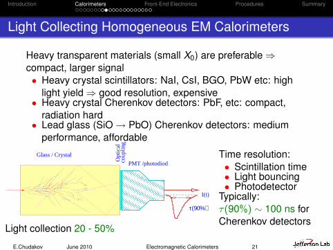
Light Collecting Homogeneous EM Calorimeters

Heavy transparent materials (small X0) are preferable ⇒compact, larger signal• Heavy crystal scintillators: NaI, CsI, BGO, PbW etc: high

light yield ⇒ good resolution, expensive• Heavy crystal Cherenkov detectors: PbF, etc: compact,

radiation hard• Lead glass (SiO → PbO) Cherenkov detectors: medium

performance, affordable

��

��

��

��

Glass / Crystal

Opt

ical

coup

ling

τ(90%)

I(t)

PMT /photodiod

Light collection 20 - 50%

Time resolution:• Scintillation time• Light bouncing• Photodetector

Typically:τ(90%) ∼ 100 ns forCherenkov detectors



Light Collecting Sampling EM Calorimeters

Heavy absorber (Pb,Cu,W...) and a scintillator (plastic) orCherenkov radiator (quartz fibers ...). Problem: how to collectthe light? The most popular solutions for this moment:• SPACAL (Pb, sc. fibers). The fibers can be bundled to the

PM. Very good resolution. Difficult to manufacture.• Sandwich with WLS fibers crossing through (“shashlik”).

The fibers are bundled to the PM. Good resolution. Easy tobuild.

Pb Pb Pb Pb PbSc Sc Sc Sc Sc

WLS fibers

PMT

Time resolution:• Scintillation time• Photodetector time

Typicallyτ(90%) ∼ 50 ns



Light Detectors

Photomultiplier Tubes (PMT)A vacuum vessel with aphotocathode and a set ofelectrodes (dynodes) forelectron multiplication.• Very high gain ∼ 105 − 107

• Very low electronic noise• Size: diameter 2-40 cm• • Slow drift of the gain• • Sensitive to the magnetic

field• • Relatively low QE∼20%• Radiation hard

Avalanche Photodiods (APD)A silicon diod in avalanche modeand an electronic amplifier• Gain ∼ 50− 300• • High electronic noise• • Size: 1× 2 cm2

• • Very sensitve to the biasvoltage

• Not sensitive to the magneticfield

• High QE∼75% at 430 nm• • Temperature sensitive

-2%/K• • Radiation hardness may be

a problem



Crystals in big experiments

BaBar CsI(Tl) ∼ 10000

L3 BGO - ∼ 11000

CMS PbWO - ∼ 80000



EM calorimeters with optical readout

Density X0 RM λI Refr. τ Peak Light Np.e.

GeV rad σEE

Material g/cm3 cm cm cm index ns λ nm yieldCrystals

NaI(Tl)∗∗ 3.67 2.59 4.5 41.4 1.85 250 410 1.00 106 102 1.5%/E1/4

CsI ∗ 4.53 1.85 3.8 36.5 1.80 30 420 0.05 104 104 2.0%/E1/2

CsI(Tl)∗ 4.53 1.85 3.8 36.5 1.80 1200 550 0.40 106 103 1.5%/E1/2

BGO 7.13 1.12 2.4 22.0 2.20 300 480 0.15 105 103 2.%/E1/2

PbWO4 8.28 0.89 2.2 22.4 2.30 5/39% 420 0.013 104 106 2.0%/E1/2

15/60% 440100/01%

LSO 7.40 1.14 2.3 1.81 40 440 0.7 106 106 1.5%/E1/2

PbF2 7.77 0.93 2.2 1.82 Cher Cher 0.001 103 106 3.5%/E1/2

Lead glassTF1 3.86 2.74 4.7 1.647 Cher Cher 0.001 103 103 5.0%/E1/2

SF-5 4.08 2.54 4.3 21.4 1.673 Cher Cher 0.001 103 103 5.0%/E1/2

SF57 5.51 1.54 2.6 1.89 Cher Cher 0.001 103 103 5.0%/E1/2

Sampling: lead/scintillatorSPACAL 5.0 1.6 5 425 0.3 2 · 104 106 6.0%/E1/2

Shashlyk 5.0 1.6 5 425 0.3 103 106 10.%/E1/2

Shashlyk(K) 2.8 3.5 6.0 5 425 0.3 4 · 105 105 3.5%/E1/2

∗ - hygroscopic



Crystal Ball (SLAC, DESY)

• ∼ 600 NaI crystals• γ detection• Charmonia spectra⇒ QCD tune!



KTeV (FNAL)

• 3256 CsI crystals

• π◦ → γγ detection

• σE/E ≈ 2.0%√

E + 0.5%



BaBar (SLAC)

Figure 3: The BABAR Detector. 1. Silicon Vertex Tracker (SVT), 2. Drift Chamber (DCH),

3. Particle Identi�cation Subsystem (DIRC{Detector of Internally Re ected Cherenkov Light, 4.

Electromagnetic Calorimeter (EMC), 5. Magnet, 6. Instrumented Flux Return (IFR).

the B1 permanent magnets at �20 cm from the interaction point, which separate the beams after

head-on collisions. The acceptance in polar angle � is limited by the gap between beamline elements

to �0:87 < cos �lab < 0:96 (�0:95 < cos �cm < 0:87). As the innermost BABAR subdetector, two

important considerations in optimizing the design were low mass, to minimize multiple scattering,

and radiation hardness of its components. A detailed description of the SVT and its components

can be found in Ref. [4].

The SVT contains 52 modules built out of AC-coupled double-sided silicon sensors (strips

othogonal on the two sides). These are read out by a full-custom low-noise radiation-hard integrated

circuit, known as the AtoM chip (mounted on a passive hybrid circuit that is attached to a water

cooling channel). The detector modules are organized in �ve radial layers, each divided azimuthally

into 6, 6, 6, 16 and 18 staves respectively (see Table 4). The three inner layers are crucial for vertex

and tracking resolution, while the outer two layers are needed to provide additional measurements

for stand alone tracking independent of drift chamber information. These outer two layers each

contain two di�erent types of modules, an inner (labelled a in the Table 4) and an outer (labelled

b) layer, occupying slightly di�erent radial positions. The modules are assembled on carbon �ber

support cones, which in turn are positioned around the beam pipe and the B1 magnets. The SVT

and some beamline elements are housed inside a strong support tube, with its load transferred at

the ends to the PEP-II beamline support \rafts."

• ∼ 10000 CsI(Tl) crystals

• σE/E ≈ 2.3%/E1/4 + 1.9%

and digitizing electronics provide for a total of four overlapping linear ranges. The system handles

signals from �50 keV to �13GeV, corresponding to 18 bit dynamic range. A short shaping time

of � 400 ns is used in the preampli�ers to reduce the impact of soft (<5MeV) beam-related pho-

ton backgrounds. Noise performance can be recovered by digitally processing the signal waveform

sampled at 4MHz. Calibration and monitoring is achieved by charge injection into the front end

of the preampli�ers, a �beroptic/xenon pulser system injecting light into the rear of each crystal,

and a circulating radioactive source (a neutron-activated uorocarbon uid) producing a 6.13MeV

photon peak in each crystal. Signals from data (�0s, �s, radiative, and non-radiative Bhabhas,

and �+�� events) can provide additional calibration points. Source and Bhabha calibrations

are updated weekly to track the small changes in light yield with integrated radiation dose. Light

pulser runs are carried out daily to monitor relative changes at the <0.3% level.

The calorimeter has achieved an electronics noise energy (ENE) of �220 keV (coherent plus

incoherent) measured with the source system (in the absence of colliding beams) after digital signal

processing. During regular data taking, this digital �ltering is not applied and the ENE rises to

�450 keV owing to the short shaping time; consequently, only channels with >1MeV are presently

used in the reconstruction of calorimeter energy deposits. The e�ciency of the calorimeter exceeds

96% for the detection of photons with energies above 20MeV.

The energy resolution can be measured directly with the radioactive source at low energies and

with electrons from Bhabha scattering at high energies, yielding resolutions of �(E)=E = 5:0�0:8%at 6.13MeV and �(E)=E = 1:9 � 0:07% at 7.5GeV, respectively. The energy resolution can also

be inferred from the observed mass resolutions for the �0 and �, which are measured to be around

7MeV and 16MeV, respectively.

/ GeVγ

E10-2

10-1

1

(E

) / E

σ

0

0.01

0.02

0.03

0.04

0.05

0.06

0.07

2σ⊕1/4/E1σ(E)/E = σ

0.3)%± 0.03 ± = (2.32 1σ

0.1)%± 0.07 ± = (1.85 2σ

γγ→0πγγ→η

Bhabhasγψ J/→cχ

radioakt. SourceMonteCarlo

Figure 8: The energy resolution as a function of energy, as determined from the observed width

of �0 and � decays to two photons of equal energy, and the resolution for Bhabha electrons. The

shaded band is the best �t to the �0, �, and Bhabha data. Also shown is the energy resolution of

the 6.13MeV photons from the radioactive source, and of the photons in the transition �c1 ! J= .E.Chudakov June 2010 Electromagnetic Calorimeters 28


SpaCal (CERN, Frascatti, JLab)

scintillating fibers / lead matrix

• Fibers/lead 50% / 50% involume

• X◦ = 1.2 cm• 5 g/cm3

• CERN - original R&D

• KLOE (DAFNE) - 5000 PMTs

• KLOE σE/E ≈ 5.7%/E1/2

• KLOE στ ≈ 50/E1/2 + 50 ps



SpaCal: Barrel Calorimeter in Hall D

target. The target is surrounded by a start counter made of plastic

scintillator that provides event timing information, a cylindrical

tracking chamber (CDC) and a cylindrical electromagnetic calori-

meter (BCAL). Downstream of the target are circular planar

tracking chambers (FDC) and a circular planar electromagnetic

calorimeter (FCAL). A schematic of the detector is shown in Fig. 1;

the two electromagnetic calorimeters are used to detect and

determine the four-momentum of the aforementioned decay

photons.

The BCAL is shown schematically in Fig. 2. The dimensions of

this calorimeter are driven by the volume required for charged

particle tracking and the bore dimensions of the solenoidal

magnet. The BCAL design is based on that of the electromagnetic

calorimeter used in the KLOE experiment at DAFNE-Frascati,

ARTICLE IN PRESS

560 cm

342 cm48 cm

185 cm

CDC

Central Drift Chamber

FDC

Forward Drift Chambers

Solenoid

Future

Particle ID

photon

beam

BCAL

Barrel Calorimeter

FCAL

Forward

Calorimeter

Solenoid

Target

Fig. 1. Schematic of the GlueX detector. The detector has cylindrical symmetry about the beam direction. The detector subsystems and the dashed lines at angles

(with respect to the beam direction) 10:8–126:4� are referenced in the text. The start counter is not shown for clarity.

11.77 cm

8.51 cm

22.46 cm

BCAL end view

BCAL top half cutaway

single module

end

Readout:

4 X 6 + 2 X 2

= 28 segments

per end

65 cm

25 cm

48m

odules

390 cm

180

cm 30-cm targetbeamline

BCAL

11°126°

390 cm

65 cmBCAL

Fig. 2. The GlueX BCAL. (a) BCAL schematic; (b) a BCAL module side view; (c) end view of the BCAL showing all 48 modules and (d) an end view of a module showing

read-out segmentation. Details are given in the text.

B.D. Leverington et al. / Nuclear Instruments and Methods in Physics Research A 596 (2008) 327–337328

scintillating fibres of 1mm diameter. These were bonded in the

lead channels with Bicron-6002 optical epoxy. The thickness of the

module is 23 cm, its length is 400 cm and the width is 12 cm with

the internal matrix geometry as indicated in Fig. 4. The matrix was

built upon an aluminum base plate of 2.54 cm thickness that was

further supported by a steel I-beam for added stiffness and ease of

handling. Module 1 was not machined along its long sides at the

7:5� indicated in Fig. 2 and retained its rectangular profile from

production. In contrast, the two ends of the module, where the

read-out system was attached, were machined and polished.

Visual inspection revealed that only eight of the approximately

17000 fibres had been damaged in handling and construction. No

optical defects affecting light transmission were observed in the

other fibres.

3. Beam test

The goals of the beam test were to measure the energy, timing

and position resolutions of the prototype BCAL module as well as

the response of the module at different positions along its length

and at various angles of the incident beam. Results of this beam

test will anchor further Monte Carlo simulations of the GlueX

detector and will aid in the development of the 48 modules for the

full BCAL detector. The detailed analysis and results reported in

this paper are for Module 1 perpendicular to the beam (y ¼ 90�)

with the beam incident at its centre (z ¼ 0 cm).

3.1. Experimental facility

The beam test took place in the downstream alcove of Hall B at

the Thomas Jefferson National Accelerator Facility (Jefferson Lab).

In order to accommodate the module with its support frame, read-

out system and cables, an additional platform was installed in

front of the alcove. This expanded space allowed for the

measurements with the photon beam perpendicular to the

module, as well as providing a greater range of lateral and

rotational degrees of freedom for the module when positioned

inside the alcove. However, as illustrated in Fig. 5, the relative

dimensions of the alcove and platform, with respect to the length

of the module, still allowed for only a limited range of positions

and incident angles that could be illuminated by the beam.

Measurements, when the module was on the platform and

oriented perpendicularly to the beam, were possible for relative

positions of the beam spot between ÿ100 to þ25 cm with respect

to the centre of the module. Within the alcove, the angular range

was limited to angles 40� and less, and a length scan was carried

out between ÿ190 to ÿ15 cm. The module was mounted on a cart

that could be remotely rotated with good precision to the required

angle. Lateral movements of the module with respect to the beam

required a hall access for manual positioning.

The primary electron beam energy from the CEBAF accelerator

at Jefferson Lab was E0 ¼ 675MeV and the current was 1nA for

most of the measurements. The electron beam was incident on a

ARTICLE IN PRESS

Table 1

BCAL properties

Property Value Ref.

Number of modulesa 48

Module lengtha 390 cm

Module inner corda 8.51 cm

Module outer corda 11.77 cm

Module thicknessa 22.5 cm

Module azimuthal bitea 7:5�

Radial fibre pitchb 1.22mm

Azimuthal fibre pitchb 1.35mm

Lead sheet thicknessc 0.5mm

Fibre diameterc 1.0mm [7]

First cladding thicknessc 0.03mm [7]

Second cladding thicknessc 0.01mm [7]

Core fibre refractive indexc 1.60 [7]

First cladding refractive indexc 1.49 [7]

Second cladding refractive indexc 1.42 [7]

Trapping efficiencyc,d,e 5.3% (min) 10.6% (max) [7–9]

Attenuation lengthbð307� 12Þ cm [10]

Effective speed of lightb, ceff ð16:2� 0:4Þ cm=ns [10]

Volume ratiosb 37:49:14 (Pb:SF:Glue) [11]

Effective mass numbere 179.9 [11]

Effective atomic numbere 71.4 [11]

Effective densitye 4:88g=cm3 [11]

Sampling fractionf 0.125 [12]

Radiation lengthe7.06 g/cm2 or 1.45 cm [11]

Number of radiation lengthse 15:5X0 (total thickness) [11]

Critical energye 11.02MeV (8.36MeV) [13,14]

Location of shower maximume 5.0X0 (5.3X0) at 1GeV [13,14]

Thickness for 95% containmente 20.3X0 (20.6X0) at 1GeV [13,14]

Moliere radiuse 17:7g=cm2 or 3.63 cm [14]

Energy resolutionb, sE=E 5:4%=ffiffiffi

Ep

� 2:3%

Time difference res.b, sDT=2 70ps=ffiffiffi

Ep

z-position resolutionb, sz 1.1 cm/ffiffiffi

Ep

(weighted)

Azimuthal angle resolutionf�8:5mrad

Polar angle resolutionf�8mrad

The number of radiation lengths as well as the resolutions in the table are all at

y ¼ 90� incidence.a Design parameters of the BCAL specified for the final detector.b Quantities that have been measured.c Specifications from the manufacturer.d From literature.e Parameter calculated from known quantities.f Parameter estimated from simulations.

0.5mm

1.35 mm

ratio of areas in rectangle

Pb:SciFi:Glue = 37:49:14

azimuthal

direction

rad

ial d

ire

ctio

n

1.2

2 m

m0

.23

3 m

m

0.053 mm

(glue ring)

SciFi

Pb

Glue

Fig. 4. The BCAL fibre matrix showing the placement of 1mm diameter fibres in

the azimuthal and radial directions. The dimensions of the azimuthal and radial

pitch, the glue box between the lead sheets and the glue ring around the fibres

were determined from the prototype module using a measuring microscope.

Particle tracks would appear to enter the matrix from the bottom. More details are

given in Ref. [11].

2 Saint-Gobain Crystals & Detectors, USA (www.bicron.com).

B.D. Leverington et al. / Nuclear Instruments and Methods in Physics Research A 596 (2008) 327–337330



SpaCal: Barrel Calorimeter in Hall D

Built at Regina

Lead swaging (grooves)Glue lead and fibers layerby layerCut and polish



Barrel Calorimeter - Construction of Modules

40 modules built

very regular matrix a ruler at the opposite sideis seen through the fibers



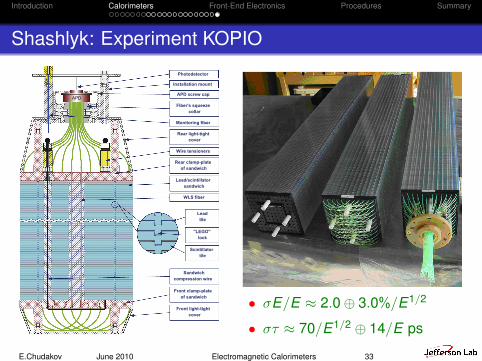
Shashlyk: Experiment KOPIO

tile exposed to collimated 90Sr electrons. For comparison,the simulated light collection efficiencies are shown. Onecan see that there is consistency between the opticalsimulations and measurements. Further improvementcould be achieved if Millipore paper with reflectionefficiency of 90% were used [11].

2.3. WLS fibers

A main concern about the WLS fibers for the Shashlykreadout is the light attenuation length in a fiber. Long-

itudinal fluctuations of electromagnetic showers are about3–4cm (one radiation length). The effective attenuationlength in fibers, including the effect of the fiber loop and thecontribution of the short-distance component of light, mustbe greater than 3–4m to have this contribution to the energyresolution be much smaller than the sampling contribution.We have measured (see Fig. 4) the light attenuation in

few multi-clad WLS fibers using a 1� 1 cm2 wide muonbeam penetrating the module transversely.The effective attenuation length of 3.6m in Kuraray

Y11(200)MS fiber satisfies our requirements. In comparison

ARTICLE IN PRESS

APD

Rear light-tight

cover

Sandwich

compression wire

Photodetector

Monitoring fiber

Fiber's squeeze

collar

Front clamp-plate

of sandwich

Front light-tight

cover

"LEGO"

lock

APD screw cap

Installation mount

Rear clamp-plate

of sandwich

Wire tensioners

WLS fiber

Scintillator

tile

Lead

tile

Lead/scintillator

sandwich

Fig. 1. The Shashlyk module design.

G.S. Atoian et al. / Nuclear Instruments and Methods in Physics Research A 584 (2008) 291–303 293

with other fibers, this commercial fiber also provides the bestreemission efficiency of blue scintillation light, and hasexcellent mechanical properties, high tensile and bendingstrength, and high uniformity in cross-sectional dimensions.For example, its light reemission efficiency is a factor of 1.5larger than that for tested Bicron WLS fiber, and thediameter for any round fiber is more uniform than others inthat it varies by no more than 2.0%.

2.4. Scintillator

An important contribution for the improvement of thephoto-statistics over earlier designs of Shashlyk modules is

the use of new scintillator tiles with an increased lightcollection efficiency. An optimization of the light yield ofthe scintillator tiles for the KOPIO Shashlyk modules hasbeen developed and carried out at the IHEP scintillatorfacility (Protvino, Russia) [9]. In the previous Shashlykcalorimeters, scintillator based on PSM115 polystyrenewas used. The new modules employ BASF143E-basedscintillator.Though there is no actual increase in the amount of light

produced by a charge particle, the light collection efficiencyin the new scintillator tile has a gain by a factor of 1.6.Because the index of refraction for the polystyrene-basedscintillator is 1.59, only light from total internal reflectionon the large side of the scintillator tile can be captured by aWLS fiber. The total internal reflection efficiency can

ARTICLE IN PRESS

Fig. 2. The Shashlyk modules at different stages of assembly.

Table 1

Parameters of the improved Shashlyk module

Transverse size 110� 110mm2

Scintillator thickness 1:5mm

Spacing between scintillator tiles 0:350mm

Lead absorber thickness 0:275mm

Number of the layers 300

WLS fibers per module 72� 1:5m ¼ 108m

Fiber spacing 9:3mm

Hole diameter (lead/scintillator) 1.3mm

Diameter of WLS fiber (Y11-200MS) 1.0mm

Fiber bunch diameter 14.0mm

External wrapping (TYVEK paper) 150mmEffective radiation length, X 0 34.9mm

Effective Moliere radius, RM 59.8mm

Effective density 2:75 g=cm3

Active depth 555mm ð15:9X 0Þ

Total depth (without photo-detector) 650mm

Total weight 21 kg

90

95

100

105

110

-50 0 50

X coordinate, mm.

Lig

ht c

olle

ctio

n ef

ficie

ncy,

a.u

.

The fiber position

εR = 0.90

εR = 0.80

εR = 0.65

Regular TYVEK paper

XEROX copier paper

Fig. 3. The dependence of the light collection efficiency in the scintillator

tile on the x-coordinate of the point-like light source. Solid lines are the

simulations for the specified reflection efficiencies eR of the wrapping

material.

0.7

0.8

0.9

1

0 20 40 60

x, cm

Lig

ht o

utpu

t, a.

u.

Y11(200)MS, λ=360 cmY11(200)M, λ=304 cmBCF-99-29AA, λ=195 cm

Fig. 4. The effective attenuation of the light in the fibers of Shashlyk

module. Experimental data (marks) are fit by the exponential dependence

expð�x=lÞ (solid lines), where x is the distance to the photo-detector and lis the effective attenuation length.

G.S. Atoian et al. / Nuclear Instruments and Methods in Physics Research A 584 (2008) 291–303294

• σE/E ≈ 2.0⊕ 3.0%/E1/2

• στ ≈ 70/E1/2 ⊕ 14/E ps



Front-End Electronics

Requirements

• Resolution ∼ 10−3

• Dynamic range > 102:needed to measure theshower profile and thecoordinates

• Differential linearity <1%• Digitization speed (>1 MHz)• Readout speed (>100 kHz)• Cost

Existing generic solutions

• Charge integrating ADC• Flash ADC• Combinations (pipeline ADC)



Charge Integrating ADC

Q→VC

inpu

t

out

gate

+

−

Q V V T TDC

gate

inpu

t

100ns

10us

DAQ

Integrating ADC

• Many products on the market• Precise: 12-15 bits• Gate must come in time ⇒ long(>300-500 ns) delay for eachchannel is needed (cables)• Slow conversion time > 10 µs ⇒not suitable for trigger logic• Problems at very high rate:pileup, deadtime• Pedestal



Flash ADC

* *

*

** *

*

**

* * *

inputV

digi

tal t

empe

ratu

re c

ode

enco

der

sam

plin

g mem

ory

1

1

0

0

0

n−bits

11

2

2n−1

2 ns = 500 MHz

Flash ADC

+

−

+

−

+

−

+

−

+

−

• Cost ×10 of the QDC(250 MHz, 12 bits)• Huge memory buffers needed• Resolution n bits ⇒ 2n

comparators• Pipeline readout - no dead time• No delay cables needed• Pileup can be partially resolved• Time resolution without extradiscr.& TDCs• FPGA computing - trigger logic• Became the mainstream



Calibration

The detector has to be calibrated atleast once.• Test beam• Better: in-situ, using an

appropriate process:◦ e+e− collider: Bhabha

scattering e+e−→ e+e−,e+e−→ e+e−γ

◦ LHC: Z→e+e− (1 Hz at lowluminocity)

◦ h+h→π0+X, π0 → γγ◦ RCS (JLab): e−p→e−p

Procedure: for event n:

E(n) =∑

i∈k×k

αi · A(n)i

χ2 =∑

n

(E (n) −∑

i∈k×k

αi · A(n)i )/σn

• System of linear equations• ⇒ N×N matrix - nearly diagonal• Easy to solve



Monitoring

Instabilities:• All avalanche-type devices tend to drift (PMT, gas

amplification ...)• Optical components may lose transparency• Temperature dependence• Many other sources of instability ...

Calibration is typically done once per many days of running ⇒signal monitoring in between is needed.



Light collecting devices

��

��

X

Stable light source

Opticalfibers

pulsed

Luc

ite p

late

Calorimeter

Stable light source

optical fibers

pulsed

lightscattering

• Stable pulsed light source:◦ Xe flash lamp: 1% stability, >100 ns

pulse◦ Laser: 2-5% stability, �1 ns pulse◦ LED: 1-3% stability in thermostate,

>30 ns pulse• Usually the light source has to be

monitored• Light distribution• Material transparency: not easy to

monitor (λ-dependence)• Scintillation yield - no monitoring this

way



Summary

Calorimeters are used for:Detecting neutralsEnergy and coordinate measurementsTriggerSeparation of hadrons against e±, γ and muons

The calorimeters are of increasing importance with higherenergies. They became the most important/expensive/largedetectors in the current big projects (LHC etc).



Summary (continued)

There are various techniques to build calorimeters for differentresolution, price, radiation hardness and other requirements.

The typical energy resolutions are:• EM: from σE

E ∼ 2%√E⊕ 0.3% for scintillating crystals to about

σEE ∼ 10%√

E⊕ 0.8% for sampling calorimeters.

• HD calorimeters: σEE ∼ 30−50%√

E⊕ 3%

The coordinate resolutions could be about 1-3 mm for EMcalorimeters and 20-30 mm for HD ones.


electromagnetic calorimeters...affordable adc (analog-to-digital converters). new accelerators -...

Documents